
1
Computational Comparison of Five Maximal Covering Models for
Locating Ambulances
Version 2
May 31, 2007
Erhan Erkut1
Armann Ingolfsson2
Thaddeus Sim3
Güneş Erdoğan4
1Faculty of Business Administration
Bilkent University
Ankara, Turkey
2School of Business
University of Alberta
Edmonton, Alberta, Canada
3Department of Management Sciences
Tippie College of Business
University of Iowa
Iowa City, Iowa, USA
4Department of Industrial Engineering
Bilkent University
and
Tepe Teknolojik Servisler A.S.
Ankara, Turkey

2
Abstract
We categorize existing maximum coverage optimization models for locating
ambulances based on whether uncertainty about (1) ambulance availability and
(2) response times is incorporated. We use data from Edmonton, Alberta, Canada
to test five different models, using the approximate hypercube model to compare
solution quality between models. We find that the basic maximum covering
model which ignores these two sources of uncertainty generates solutions that
perform far worse than those generated by more sophisticated models. The
model that incorporates both sources of uncertainty generates a configuration that
covers up to 26% more than the demand covered by the basic model with the
same number of ambulances.
3
1. Introduction
Emergency Medical Services (EMS) must balance cost and quality of service when planning
their operations. Quality of service has multiple attributes, including response times, the type of
care that EMS staff are trained to provide, and the equipment to which they have access. We
will focus on response time—the time from contacting EMS until the patient is reached.
Response time performance is typically measured as a cumulative fraction (referred to as the
fractile method of reporting), for example the fraction of life-threatening calls reached in 8:59
minutes or less. Such performance measures are recommended by industry experts (Fitch, 2005)
and in standards prepared by the National Fire Protection Association (2004, section 5.3.3.4.3).
Regulations based on the EMS Act of 1973 in the US specified that 95% of calls should be
reached in 10 minutes (Revelle, et al., 1977). A 2004 survey of the 200 largest cities in the US
indicated that over three quarters of EMS agencies that provide transport to hospital use a target
of 8:59 minutes or less and report the fraction of calls reached within this time standard (as
opposed to, say, the average response time). The single most common standard for urban areas,
at least in North America, appears to be to reach 90% of life-threatening calls in 8:59 minutes or
less (Fitch, 2005).
Given the nature of such performance standards, it is not surprising that location theorists have
formulated optimization problems to locate a fixed number of ambulance stations and to allocate
a fixed number of ambulances to stations so as to optimize either (1) the average response time
or (2) the demand that can be reached within some time standard. These two performance
measures were discussed in an early survey paper by Chaiken and Larson (1972) and both
measures have an associated stream of research in the operations research and location theory
literature.
Jarvis (1975) developed the best known approach to minimizing measure (1), the average
response time—a locate-allocate heuristic that use the approximate hypercube model (Larson,
1975) to evaluate solutions. We focus primarily on measure (2) because it corresponds to the
measurement standard that is predominant in current practice. Research that focuses on measure
(2) uses the concept of coverage, where a demand location is assumed to be covered by an
ambulance station if the distance (or travel time) between the two is less than or equal to some
threshold.
The first paper on locating EMS units optimally introduced the set covering location model
(Toregas et al., 1971). This is a binary programming model which finds the minimum number of
EMS units required to cover all demand locations in the service area. Unfortunately the optimal
solution to this model requires an excessive number of EMS units since it requires complete
coverage and disregards the cost of the system. Church and ReVelle (1974) proposed a more
practical alternative: the maximal covering location problem (MCLP). The maximal covering
location model fixes the number of EMS stations, and seeks to maximize the coverage of
demand points in the service area. The binary integer program can be solved relatively easily
using commercial software as its LP relaxation usually produces all-integer solutions. It has
been used in practice for locating ambulance stations (Eaton et al., 1985), and it may be the most
influential of all ambulance station location models.
4
Despite its appeal due to simplicity and solvability, MCLP is imperfect. First, it assumes that
response times are known and deterministic. In reality, response times are highly uncertain
because of factors such as variable pre-travel delays, traffic congestion, weather, local events,
and hour of day. Second, MCLP assumes that the nearest EMS unit to a demand location is
always available. A unit that is responding to a call is unavailable to respond to a subsequent
call while it travels to the service site, provides aid on-site, transports the patient to the hospital,
and completes paper work and maintenance (cleaning and stocking of materials) on the unit.
Even though an EMS system is designed for low utilization, in most EMS systems the utilization
rates are at least 25% and assuming near-zero utilization or a large number of units at each
station is not realistic. To see how these two imperfections result in miscalculations, we present
two examples.
Example 1: Consider an ambulance station with one vehicle and two demand locations A and B,
with a response time threshold of 8 minutes. Suppose that the response time from the station to
A is N(7.5, 2.5) and the response time to B is N(8.5, 2.5), where N(µ, σ) denotes a normally
distributed random variable with mean µ and standard deviation σ. MCLP, using average travel
times, considers A to be covered and B not to be covered. However, A is covered with a
probability of 0.58 and B is covered with a probability of 0.42, if there is a unit available at the
station. Assuming Pr{ambulance busy} = 0.3, we compute the probability of coverage for A and
B as 0.405 and 0.295, a far cry from 1 and 0 as estimated by MCLP. Such miscalculations can
result in poor location selections, as illustrated in our second example.
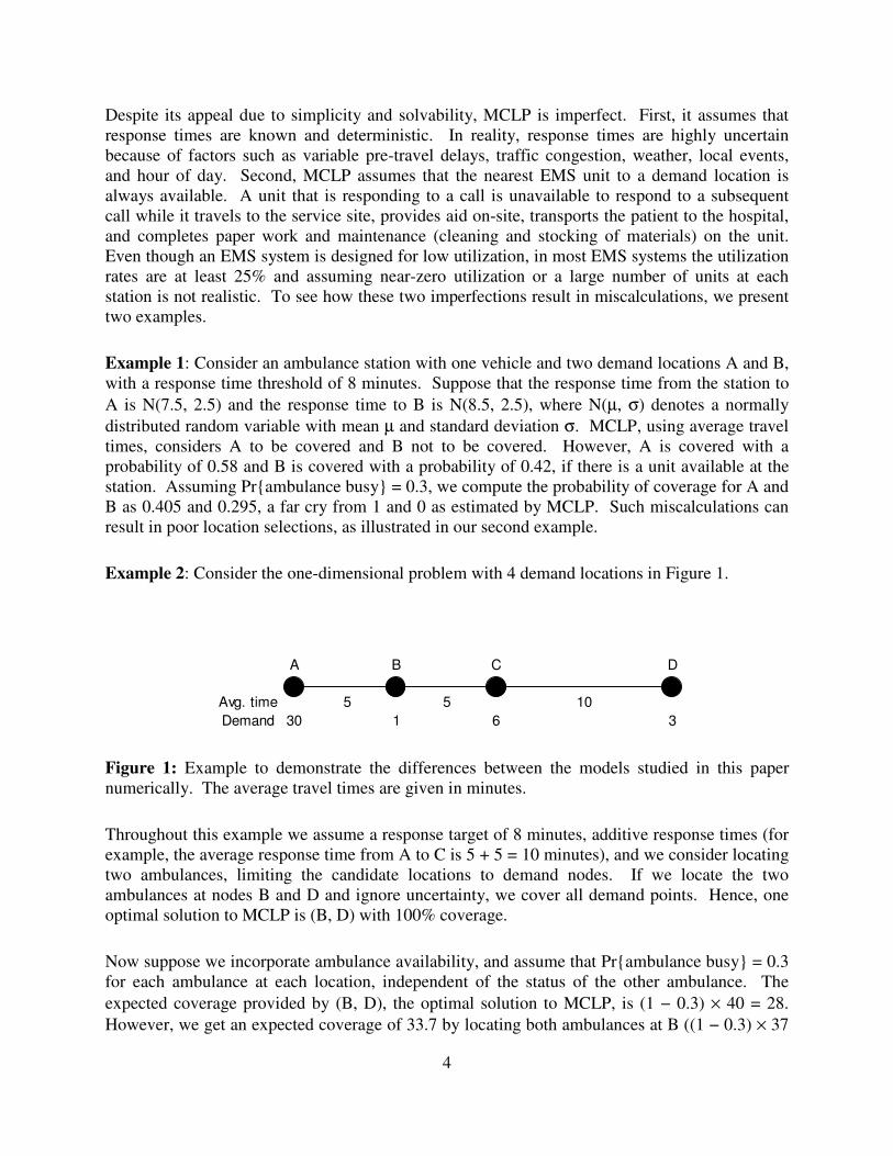
Example 2: Consider the one-dimensional problem with 4 demand locations in Figure 1.
A B C D
Avg. time 5 5 10
Demand 30 1 6 3
Figure 1: Example to demonstrate the differences between the models studied in this paper
numerically. The average travel times are given in minutes.
Throughout this example we assume a response target of 8 minutes, additive response times (for
example, the average response time from A to C is 5 + 5 = 10 minutes), and we consider locating
two ambulances, limiting the candidate locations to demand nodes. If we locate the two
ambulances at nodes B and D and ignore uncertainty, we cover all demand points. Hence, one
optimal solution to MCLP is (B, D) with 100% coverage.
Now suppose we incorporate ambulance availability, and assume that Pr{ambulance busy} = 0.3
for each ambulance at each location, independent of the status of the other ambulance. The
expected coverage provided by (B, D), the optimal solution to MCLP, is (1 − 0.3) × 40 = 28.
However, we get an expected coverage of 33.7 by locating both ambulances at B ((1 − 0.3) × 37
5
+ 0.3 × (1 − 0.3) × 37), and this is the maximal expected coverage. This is because the majority
of the demand is at nodes A, B, and C, and the secondary coverage of these nodes provides a
higher incremental expected value than the primary coverage of node D.
Suppose we do not incorporate ambulance availability, but we model response time uncertainty.
Assume that all response times follow a lognormal probability distribution where the travel time
given in Figure 1 is equal to the mean, and the standard deviation is equal to half of the mean.
We use a lognormal instead of a normal distribution to avoid negative response times—see
further discussion in Section 4. In this case, the model protects the highest demand points by
locating the two ambulances at A and C. Finally, suppose we combine both sources of
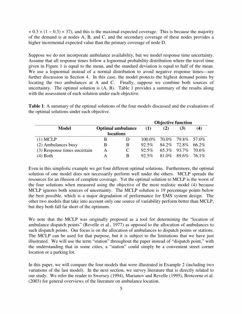
uncertainty. The optimal solution is (A, B). Table 1 provides a summary of the results along
with the assessment of each solution under each objective.
Table 1: A summary of the optimal solutions of the four models discussed and the evaluations of
the optimal solutions under each objective.
Objective function
Model Optimal ambulance
locations
(1) (2) (3) (4)
(1) MCLP B D 100.0% 70.0% 79.8% 57.0%
(2) Ambulances busy B B 92.5% 84.2% 72.8% 66.2%
(3) Response times uncertain A C 92.5% 65.3% 93.7% 70.6%
(4) Both A B 92.5% 81.0% 89.6% 76.1%
Even in this simplistic example we get four different optimal solutions. Furthermore, the optimal
solution of one model does not necessarily perform well under the others. MCLP spreads the
resources for an illusion of complete coverage. Yet the optimal solution to MCLP is the worst of
the four solutions when measured using the objective of the most realistic model (4) because
MCLP ignores both sources of uncertainty. The MCLP solution is 19 percentage points below
the best possible, which is a major degradation of performance for EMS system design. The
other two models that take into account only one source of variability perform better than MCLP,
but they both fall far short of the optimum.
We note that the MCLP was originally proposed as a tool for determining the “location of
ambulance dispatch points” (Revelle et al., 1977) as opposed to the allocation of ambulances to
such dispatch points. Our focus is on the allocation of ambulances to dispatch points or stations.
The MCLP can be used for that purpose, but it is subject to the limitations that we have just
illustrated. We will use the term “station” throughout the paper instead of “dispatch point,” with
the understanding that in some cities, a “station” could simply be a convenient street corner
location or a parking lot.
In this paper, we will compare the four models that were illustrated in Example 2 (including two
variations of the last model). In the next section, we survey literature that is directly related to
our study. We refer the reader to Swersey (1994), Marianov and Revelle (1995), Brotcorne et al.
(2003) for general overviews of the literature on ambulance location.

6
2. Related Literature
We are not the first to realize the limitations of MCLP that were illustrated in Section 1. Other
researchers have developed models that take into account the two sources of uncertainty. Daskin
(1983) proposed the maximal expected covering location problem (MEXCLP—an extension of
MCLP) to account for the probability that an EMS unit is busy. Daskin assumed the probability
p that a unit is busy is the same for every unit. Assuming that the probabilities of individual
units being busy are independent, if demand node i with call rate hi is covered by m units, the
expected coverage for node i is hi × (1 − pm). MEXCLP maximizes expected coverage over all
demand nodes and finds the optimal location for a given number of units. Unlike MCLP,
MEXCLP can locate multiple units at the same station, limited by the capacity of the station.
Given that ambulances are typically busy at least 30% of the time, MEXCLP is considerably
more realistic than MCLP. Saydam and McKnew (1985) studied the same problem and offered a
separable programming formulation that they found could solve larger instances to optimality
than Daskin’s formulation.
Daskin (1987) also worked on the second shortcoming of MCLP—deterministic response times.
In essence, MCLP is a “black-and-white” representation of reality, where all demand points
within some threshold distance are considered covered and all other points are not covered. The
extension described in Daskin (1987) incorporates probabilistic coverage by explicitly modeling
response time uncertainty. Problem data includes the probability of responding from a station to
a demand point within a given threshold time.
While the two imperfections of MCLP were treated relatively early, their combined treatment
took longer to arrive. Goldberg and Paz (1991) were the first, to our knowledge, to formulate a
mathematical program that addressed both sources of uncertainty. They allowed ambulance
busy probabilities to vary between stations and used pairwise exchange heuristics to optimize
expected coverage, as evaluated by the approximate hypercube model. Ingolfsson et al. (2006)
made the same assumptions but used a different solution heuristic—one that iterates between
solving a nonlinear integer program and the approximate hypercube model. Table 2 summarizes
the maximal covering models that we have discussed.
The MCLP (top left quadrant) is a linear integer program and is the simplest to solve. Moving to
the right or down from the top left quadrant incorporates more reality into the model at the
expense of solving a more complex optimization model.
There is another stream of related research on optimization models that attempts to maximize
demand that is “covered with α-reliability,” for example, Revelle and Hogan (1989). Borras and
Pastor (2002) compare four such maximum availability models. Their work is similar to ours in
that they use the approximate hypercube model to evaluate solutions to idealized optimization
models. In a follow-on paper, Borras and Pastor (2003) present a maximum availability model
that is solved by iterating between solving an optimization problem and evaluation with the
approximate hypercube model—an approach that is similar to the one we use to solve maximum
expected coverage models. As discussed in Erkut et al. (2006), the objective function of
maximum availability models does not correspond directly to the performance measures used in
7
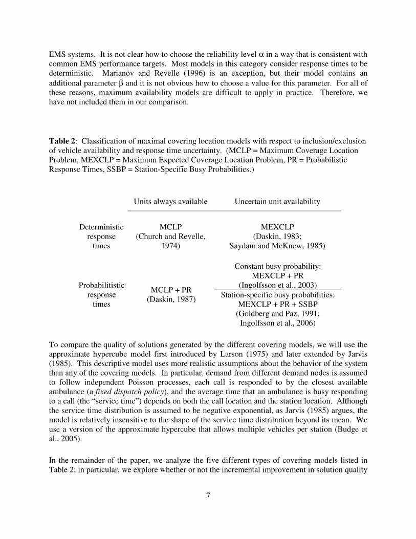
EMS systems. It is not clear how to choose the reliability level α in a way that is consistent with
common EMS performance targets. Most models in this category consider response times to be
deterministic. Marianov and Revelle (1996) is an exception, but their model contains an
additional parameter β and it is not obvious how to choose a value for this parameter. For all of
these reasons, maximum availability models are difficult to apply in practice. Therefore, we
have not included them in our comparison.
Table 2: Classification of maximal covering location models with respect to inclusion/exclusion
of vehicle availability and response time uncertainty. (MCLP = Maximum Coverage Location
Problem, MEXCLP = Maximum Expected Coverage Location Problem, PR = Probabilistic
Response Times, SSBP = Station-Specific Busy Probabilities.)
Units always available Uncertain unit availability
Deterministic
response
times
MCLP
(Church and Revelle,
1974)
MEXCLP
(Daskin, 1983;
Saydam and McKnew, 1985)
Constant busy probability:
MEXCLP + PR
(Ingolfsson et al., 2003) Probabilitistic
response
times
MCLP + PR
(Daskin, 1987) Station-specific busy probabilities:
MEXCLP + PR + SSBP
(Goldberg and Paz, 1991;
Ingolfsson et al., 2006)
To compare the quality of solutions generated by the different covering models, we will use the
approximate hypercube model first introduced by Larson (1975) and later extended by Jarvis
(1985). This descriptive model uses more realistic assumptions about the behavior of the system
than any of the covering models. In particular, demand from different demand nodes is assumed
to follow independent Poisson processes, each call is responded to by the closest available
ambulance (a fixed dispatch policy), and the average time that an ambulance is busy responding
to a call (the “service time”) depends on both the call location and the station location. Although
the service time distribution is assumed to be negative exponential, as Jarvis (1985) argues, the
model is relatively insensitive to the shape of the service time distribution beyond its mean. We
use a version of the approximate hypercube that allows multiple vehicles per station (Budge et
al., 2005).
In the remainder of the paper, we analyze the five different types of covering models listed in
Table 2; in particular, we explore whether or not the incremental improvement in solution quality
8
justifies the added model complexity. We compare the performance of the five model types
using data from the EMS system of Edmonton, Canada.
We present the formulations for the five model types in Section 3. Section 4 describes how the
busy and coverage probabilities for the EMS units can be computed. Experimental results are
provided in Section 5, and concluding remarks are given in Section 6.
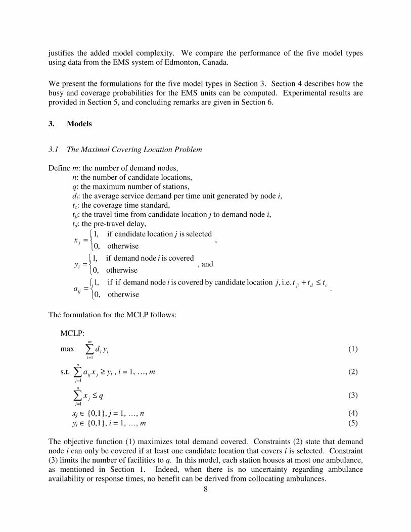
3. Models
3.1 The Maximal Covering Location Problem
Define m: the number of demand nodes,
n: the number of candidate locations,
q: the maximum number of stations,
di: the average service demand per time unit generated by node i,
tc: the coverage time standard,
tji: the travel time from candidate location j to demand node i,
td: the pre-travel delay,
=otherwise,0
selected islocation candidate if,1 j x j ,
=otherwise,0
covered is node demand if,1 iyi , and
≤+
=otherwise,0
i.e. ,location candidateby covered is node demand ifif,1 cdji
ij
tttjia .
The formulation for the MCLP follows:
MCLP:
max ∑=
m
i
ii yd1
(1)
s.t. ∑=
n
j
jij xa1
≥ yi , i = 1, …, m (2)
∑=
n
j
jx1
≤ q (3)
xj ∈ {0,1}, j = 1, …, n (4)
yi ∈ {0,1}, i = 1, …, m (5)
The objective function (1) maximizes total demand covered. Constraints (2) state that demand
node i can only be covered if at least one candidate location that covers i is selected. Constraint
(3) limits the number of facilities to q. In this model, each station houses at most one ambulance,
as mentioned in Section 1. Indeed, when there is no uncertainty regarding ambulance
availability or response times, no benefit can be derived from collocating ambulances.
9
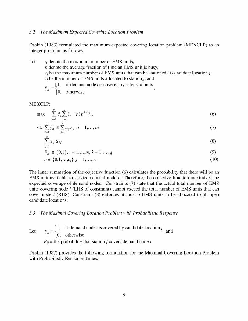
3.2 The Maximum Expected Covering Location Problem
Daskin (1983) formulated the maximum expected covering location problem (MEXCLP) as an
integer program, as follows.
Let q denote the maximum number of EMS units,
p denote the average fraction of time an EMS unit is busy,
cj be the maximum number of EMS units that can be stationed at candidate location j,
zj be the number of EMS units allocated to station j, and
=otherwise,0
units least at by covered is node demand if,1ˆ
kiyik .
MEXCLP:
max ∑∑=
−
=
−q
k
ik
km
i
i yppd1
1
1
ˆ)1( (6)
s.t. ∑∑==
≤n
jjij
q
kik zay
11
ˆ , i = 1,…, m (7)
∑=
n
j
jz1
≤ q (8)
iky ∈ {0,1}, i = 1,…,m, k = 1,…, q (9)
zj ∈ {0,1,…,cj}, j = 1,…, n (10)
The inner summation of the objective function (6) calculates the probability that there will be an
EMS unit available to service demand node i. Therefore, the objective function maximizes the
expected coverage of demand nodes. Constraints (7) state that the actual total number of EMS
units covering node i (LHS of constraint) cannot exceed the total number of EMS units that can
cover node i (RHS). Constraint (8) enforces at most q EMS units to be allocated to all open
candidate locations.
3.3 The Maximal Covering Location Problem with Probabilistic Response
Let
=otherwise,0
location candidateby covered is node demand if,1 jiyij , and
Pij = the probability that station j covers demand node i.
Daskin (1987) provides the following formulation for the Maximal Covering Location Problem
with Probabilistic Response Times:
10
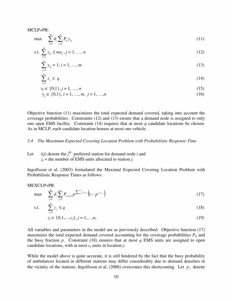
MCLP+PR:
max ∑∑==
n
j
ijij
m
i
i yPd11
(11)
s.t. ∑=
m
i
ijy1
≤ mxj , j = 1, …, n (12)
∑=
n
j
ijy1
= 1, i = 1, …, m (13)
∑=
n
j
jx1
≤ q (14)
xj ∈ {0,1}, j = 1, …, n (15)
ijy ∈ {0,1}, i = 1, …, m, j = 1, …,n (16)
Objective function (11) maximizes the total expected demand covered, taking into account the
coverage probabilities. Constraints (12) and (13) ensure that a demand node is assigned to only
one open EMS facility. Constraint (14) requires that at most q candidate locations be chosen.
As in MCLP, each candidate location houses at most one vehicle.
3.4 The Maximum Expected Covering Location Problem with Probabilistic Response Time
Let i(j) denote the jth
preferred station for demand node i and
zj = the number of EMS units allocated to station j.
Ingolfsson et al. (2003) formulated the Maximal Expected Covering Location Problem with
Probabilistic Response Times as follows:
MEXCLP+PR:
max ( ))(
1
1 )(
11
)(,
1
ji
j
u ui zzn
j
jii
m
i
i ppPd −∑−
=∑∑==
(17)
s.t. ∑=
n
j
jz1
≤ q (18)
zj ∈ {0,1,…,cj}, j = 1,…,n, (19)
All variables and parameters in the model are as previously described. Objective function (17)
maximizes the total expected demand covered accounting for the coverage probabilities Pij and
the busy fraction p. Constraint (18) ensures that at most q EMS units are assigned to open
candidate locations, with at most cj units in location j.
While the model above is quite accurate, it is still hindered by the fact that the busy probability
of ambulances located in different stations may differ considerably due to demand densities in
the vicinity of the stations. Ingolfsson et al. (2006) overcomes this shortcoming. Let jp denote

11
the average fraction of time an EMS unit at station j is busy. The formulation for the Maximal
Expected Covering Location Problem with Probabilistic Response Time and Station Specific
Busy Probabilities is as follows:
MEXCLP+PR+SSBP:
max ( ))()(
)(
1
1
)(
1
)(,
1
1 jiui z
ji
j
u
z
ui
n
j
jii
m
i
i ppPd −∏∑∑−
===
(20)
s.t. ∑=
n
j
jz1
≤ q (21)
zj ∈ {0, 1, …, cj}, j = 1, …, n (22)
Note that this model is the same as the model for MEXCLP+PR except for the busy probability
values.
3.5 Model size
Table 3 provides the number of constraints and variables for each of the five models. Although
adding more complexity to the basic MCLP model makes it more realistic, the resulting models
are either non-linear or contain more constraints and variables.
Table 3: Model dimensions.
Model Objective Constraints Variables
MCLP Linear m + 1 linear m + n binary
MEXCLP Linear m + 1 linear nm binary, n bounded integer
MCLP+PR Linear n + m + 1
linear n(m + 1) binary
MEXCLP+PR Nonlinear 1 linear n bounded integer
MEXCLP+PR+SSBP Nonlinear 1 linear n bounded integer
4. Determining Model Parameters
The optimization models presented in the previous section that involve uncertainty require input
values for the coverage probability parameter Pij, the system-wide busy fraction parameter p, and
the station specific busy fraction parameter jp . In this section, we discuss how to compute these
values. Note that the coverage probabilities Pij are true inputs, whereas the busy fractions are
outputs that depend on the allocation of ambulances to stations. We overcome this difficulty by
iterating between solving an optimization model and estimating busy fractions.
12
4.1 Coverage Probabilities
Both MCLP+PR and MEXCLP+PR require the coverage probabilities Pij as input. Although
there is no explicit station preference in MCLP+PR, we assume that the station preference for
demand node i is based on the travel time between the demand node and the stations, with the
most preferred station being the closest one.
We denote the response time for a station-node pair as Rij, with mean µij, standard deviation σij,
and coefficient of variation cij = σij / µij. The mean and standard deviation of the response time
depend on the distribution of both the travel time and the pre-travel delay. We assume that the
response times are lognormally distributed. See Ingolfsson et al. (2006) for further discussion
and empirical evidence that support the lognormality assumption. Other non-negative
distributions, such as a log-logistic distribution or a gamma distribution could be used instead.
The main consideration in choosing a distribution is to accurately model the tail probability
Pr{Rij > tc}.
If Rij is lognormally distributed, then ln(Rij) is normally distributed, with the following mean and
variance:
E[ln(Rij)] = ln(µij) - ( )21ln5.0 ijc+ , and (23)
var[ln(Rij)] = ( )21ln ijc+ , (24)
Therefore, we have
{ }
+
++µ−Φ=≤=≤=
)1ln(
)1ln(5.0)ln()ln()ln()ln(Pr}Pr{
2
2
ij
ijijc
cijcijij
c
cttRtRP (25)
where Φ is the cumulative standard Normal distribution function and tc is the coverage time
threshold.
4.2 Calculating the System-Wide Busy Fraction Parameter, p
For the models MEXCLP and MEXCLP+PR, we require the parameter p, which is the average
fraction of time that an EMS unit is busy. The average busy fraction p can be estimated as
p = λ (1 − Β(λτ(z), q)) τ(z) / q (26)
where ∑ ==
m
i id1
λ is the total arrival rate of calls to the system, τ(z) is the average time that a
vehicle is tied up with a call as a function of the vehicle allocation vector z, q is the total number
of vehicles, and 0
( , ) / ! / !ss i
iB r s r s r i
== ∑ is the Erlang loss function, which measures the
fraction of lost calls in an M/G/s/s queueing system. The total arrival rate is fixed, and the total
13
number of vehicles is fixed as well since the constraint qzm
j j ≤∑ =1 will be tight. However, the
“average service time” τ will depend on how the q vehicles are distributed across the city
because this will influence the average response time to a call. The average service time τ(z)
consists of the average response time, the average time spent at the call location, and the average
time to travel to and remain at a hospital:
τ(z) = E[Tresponse] + E[Ton scene] + E[Thospital] (27)
This assumes that the ambulance is available to take calls when it is on its way from a hospital
back to a station. Only the first component (E[Tresponse]) is assumed to depend on how vehicles
are allocated to stations. This component can be calculated as
∑∑= =
=m
i
n
j
jiiji
i Rzfd
T1 1
)(,)(response ][E)(λ
][E (28)
where fi(j)(z) is the probability that the jth
preferred station is the one that responds to a call from
demand node i. To calculate fi(j)(z), let zi(j) be the number of vehicles at the jth
preferred station
for demand node i, and we thus have
)1()( )(
1
1 )(
)(ji
j
u ui zz
ji ppzf −∑=−
= . (29)
The algorithm for iterating on the busy fraction p is as follows:
Step 0: Initialize p to pin, where pin can be determined by assuming that all calls are responded
to by the most preferred station, i.e., setting fi(1)(z) = 1 for all i (and fi(j)(z) = 0 for all j ≥
2) and then using (26), (27), and (28). Set cnt = 1 and choose a smoothing parameter γ
∈ (0,1).
Step 1: Solve the optimization model. Denote the vector of zi variables in the solution by ∗cntz .
If a convergence criterion is satisfied, stop.
Step 2: Estimate pout using the solution ∗cntz and equations (26) to (29). Set pin = γpout +
(1 - γ)pin and cnt = cnt + 1, and return to Step 1.
There are two possible ways that the algorithm may converge: first, if both the solution and the
busy fraction have converged, i.e., ∗−1cntz = ∗
cntz and |pin - pout| < ε (we used ε = 10-6). Second, if
the busy fraction has converged (i.e., |pin - pout| < ε) and the solution has converged to a repeating
cycle of solutions. In the experiments reported in the next section, the length of the cycle was at
most two.
4.3 Calculating the Station Specific Busy Fraction Parameter, jp
In model MEXCLP+PR+SSBP, we use the approximate hypercube model to estimate station
specific busy fractions. Budge et al. (2005) describe the version of the approximate hypercube

14
model that we use and Ingolfsson et al. (2006) discuss the iteration between solving the
mathematical program and estimating the busy fractions.
We made one modification to the iteration procedure described in Ingolfsson et al. (2006): if a
station was allocated no ambulances, then we set the busy probability for that station equal to the
average busy fraction for the other stations. In Ingolfsson et al. (2006), the busy probability for
such stations was set to 100%, which meant that the optimal solution to the next mathematical
program to be solved would allocate no ambulances to such stations. We found that this
modification led to higher quality solutions.
5. Computational Results
Our computational experiments were carried out on a data set provided by the EMS department
of the City of Edmonton. The data set contains expected travel times from 16 ambulance
stations to 180 demand points, and the fraction of demand generated at each of the demand
points. We limit our analysis to the 16 current ambulance stations, and focus on the allocation of
ambulances to those stations. We scaled total demand to keep the ratio between the “offered
load” (total demand per time unit multiplied by the average time per call) and the number of
EMS units equal to 0.3.
We solved the linear models using CPLEX 9.1 and the nonlinear models using the student
version of GAMS 22.0. Solving the linear models took no more than a CPU second. The
computation times and the number of iterations between solving an optimization problem and
estimating busy probabilities for the nonlinear models are shown in Table 4. The computation
times include the time to run the approximate hypercube model, which was less than one second
in all cases. The total CPU time to solve an instance varied between 4 and 659 seconds and was
highest for intermediate values of q. The number of iterations varied from 2 to 10 and was
consistently higher for the MEXCLP + PR model. The CPU time per iteration, for a given q,
was similar for the two nonlinear models.
For the system-wide busy fraction heuristic, we chose the smoothing parameter as γ = 0.8.
Notably, different values of γ did not affect the final solution. Our choices for parameters were
guided by analysis of real data. We assumed that the total average time spent at the call location,
and the average time to travel to and remain at a hospital, E[Ton scene] + E[Thospital], is 2691
seconds (about 45 minutes). When calculating the coverage probability parameter Pij, we
assumed cij = 0.3. The initial system-wide busy probability p was set to 0.3. In MCLP, we set aij
to 1 if the expected response time was less than the threshold time tc.

15
Table 4: Total CPU time (including evaluation with the approximate hypercube model) in
seconds and number of iterations for the MEXCLP+PR and MEXLPC+PR+SSBP models.
q MEXCLP+PR MEXCLP+PR+SSBP MEXCLP+PR MEXCLP+PR+SSBP
1 12 4 4 2
2 52 26 4 2
3 133 49 5 2
4 347 126 6 3
5 294 126 6 2
6 373 98 7 2
7 477 138 7 2
8 659 163 8 2
9 555 207 8 3
10 545 214 8 3
11 563 219 8 4
12 625 237 8 3
13 445 189 8 3
14 248 110 8 3
15 183 53 8 2
16 241 214 8 5
17 165 89 8 3
18 182 79 8 3
19 181 71 8 3
20 152 71 8 4
21 127 43 8 2
22 95 57 8 4
23 99 28 8 2
24 59 36 8 4
25 39 17 8 2
Total CPU time in seconds Number of iterations
We evaluated the outcome of each model by computing the dispatch probabilities fi(j)(z) for the
ambulance configuration at hand using the approximate hypercube model, and using them,
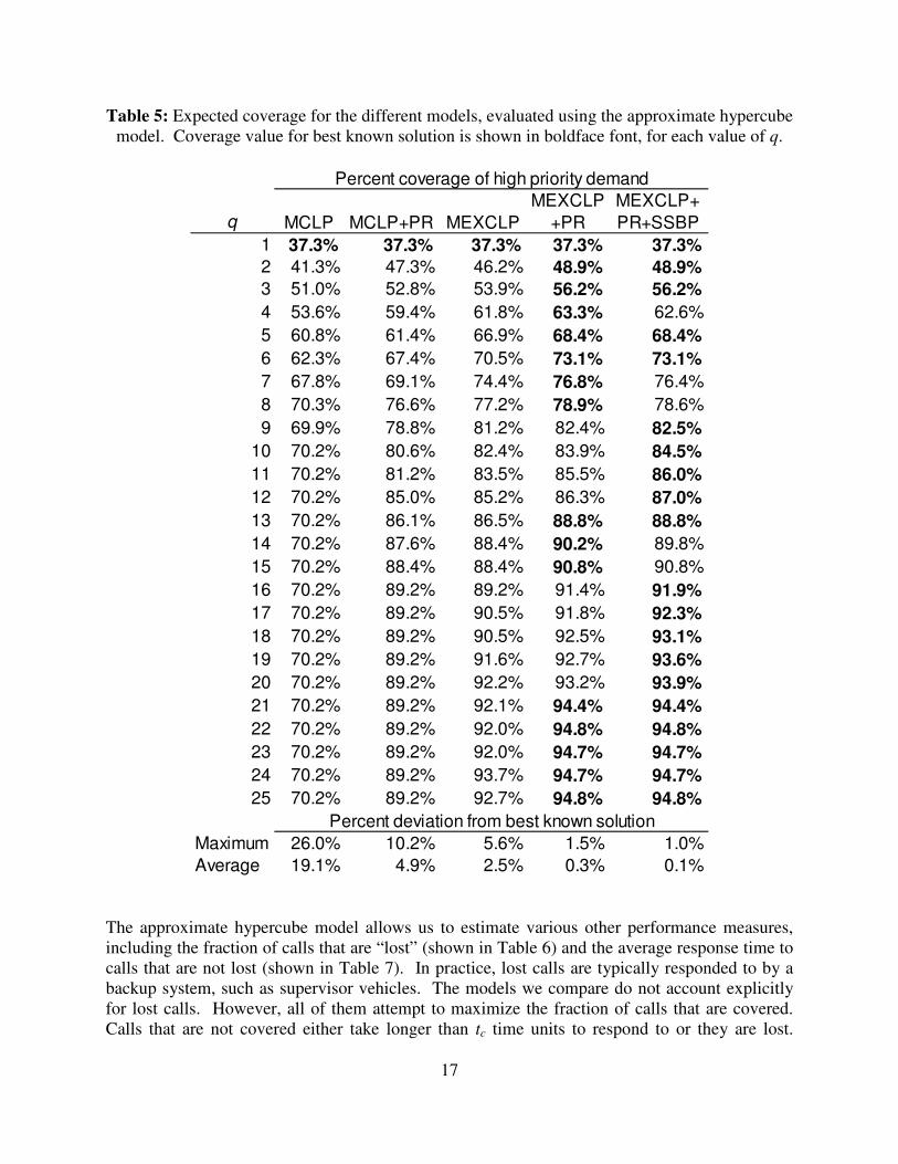
together with the coverage probabilities Pij, to compute the expected coverage. The results are
summarized in Table 5 and Figure 2. In the last row of Table 5, we show the average percent
deviation from the best solution value. Note that the maximum expected coverage that can be
achieved for the example problem on hand is 94.8%. One would need to add new station
locations to achieve greater expected coverage.
16
40%
50%
60%
70%
80%
90%
100%
1 2 3 4 5 6 7 8 9 10 11 12 13 14 15 16 17 18 19 20 21 22 23 24 25
Number of vehicles
Syste
m w
ide
co
ve
rag
e
MCLP
MCLP+PR
MEXCLP
MEXCLP+PR
MEXCLP+PR+SSBP
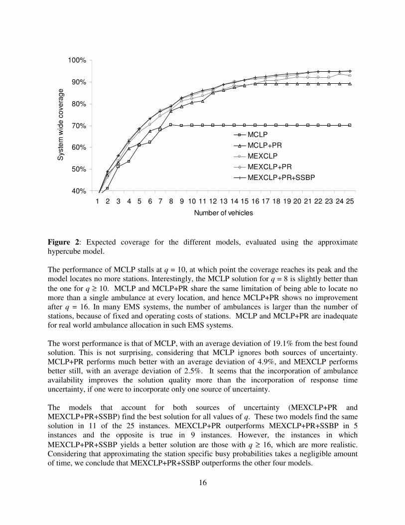
Figure 2: Expected coverage for the different models, evaluated using the approximate
hypercube model.
The performance of MCLP stalls at q = 10, at which point the coverage reaches its peak and the
model locates no more stations. Interestingly, the MCLP solution for q = 8 is slightly better than
the one for q ≥ 10. MCLP and MCLP+PR share the same limitation of being able to locate no
more than a single ambulance at every location, and hence MCLP+PR shows no improvement
after q = 16. In many EMS systems, the number of ambulances is larger than the number of
stations, because of fixed and operating costs of stations. MCLP and MCLP+PR are inadequate
for real world ambulance allocation in such EMS systems.
The worst performance is that of MCLP, with an average deviation of 19.1% from the best found
solution. This is not surprising, considering that MCLP ignores both sources of uncertainty.
MCLP+PR performs much better with an average deviation of 4.9%, and MEXCLP performs
better still, with an average deviation of 2.5%. It seems that the incorporation of ambulance
availability improves the solution quality more than the incorporation of response time
uncertainty, if one were to incorporate only one source of uncertainty.
The models that account for both sources of uncertainty (MEXCLP+PR and
MEXCLP+PR+SSBP) find the best solution for all values of q. These two models find the same
solution in 11 of the 25 instances. MEXCLP+PR outperforms MEXCLP+PR+SSBP in 5
instances and the opposite is true in 9 instances. However, the instances in which
MEXCLP+PR+SSBP yields a better solution are those with q ≥ 16, which are more realistic.
Considering that approximating the station specific busy probabilities takes a negligible amount
of time, we conclude that MEXCLP+PR+SSBP outperforms the other four models.
17
Table 5: Expected coverage for the different models, evaluated using the approximate hypercube
model. Coverage value for best known solution is shown in boldface font, for each value of q.
q MCLP MCLP+PR MEXCLP
MEXCLP
+PR
MEXCLP+
PR+SSBP
1 37.3% 37.3% 37.3% 37.3% 37.3%
2 41.3% 47.3% 46.2% 48.9% 48.9%
3 51.0% 52.8% 53.9% 56.2% 56.2%
4 53.6% 59.4% 61.8% 63.3% 62.6%
5 60.8% 61.4% 66.9% 68.4% 68.4%
6 62.3% 67.4% 70.5% 73.1% 73.1%
7 67.8% 69.1% 74.4% 76.8% 76.4%
8 70.3% 76.6% 77.2% 78.9% 78.6%
9 69.9% 78.8% 81.2% 82.4% 82.5%
10 70.2% 80.6% 82.4% 83.9% 84.5%
11 70.2% 81.2% 83.5% 85.5% 86.0%
12 70.2% 85.0% 85.2% 86.3% 87.0%
13 70.2% 86.1% 86.5% 88.8% 88.8%
14 70.2% 87.6% 88.4% 90.2% 89.8%
15 70.2% 88.4% 88.4% 90.8% 90.8%
16 70.2% 89.2% 89.2% 91.4% 91.9%
17 70.2% 89.2% 90.5% 91.8% 92.3%
18 70.2% 89.2% 90.5% 92.5% 93.1%
19 70.2% 89.2% 91.6% 92.7% 93.6%
20 70.2% 89.2% 92.2% 93.2% 93.9%
21 70.2% 89.2% 92.1% 94.4% 94.4%
22 70.2% 89.2% 92.0% 94.8% 94.8%
23 70.2% 89.2% 92.0% 94.7% 94.7%
24 70.2% 89.2% 93.7% 94.7% 94.7%
25 70.2% 89.2% 92.7% 94.8% 94.8%
Maximum 26.0% 10.2% 5.6% 1.5% 1.0%
Average 19.1% 4.9% 2.5% 0.3% 0.1%
Percent coverage of high priority demand
Percent deviation from best known solution
The approximate hypercube model allows us to estimate various other performance measures,
including the fraction of calls that are “lost” (shown in Table 6) and the average response time to
calls that are not lost (shown in Table 7). In practice, lost calls are typically responded to by a
backup system, such as supervisor vehicles. The models we compare do not account explicitly
for lost calls. However, all of them attempt to maximize the fraction of calls that are covered.
Calls that are not covered either take longer than tc time units to respond to or they are lost.

18
Therefore, one would expect that the models will tend to minimize the fraction of lost calls.
Table 6 shows that, as expected, the loss probability decreases with q, for all models. The loss
probability drops below 1% for all models for q > 9. MEXCLP+PR and MEXCLP+PR+SSBP
consistently provide the lowest loss probability.
As Table 7 shows, the average response almost always decreases with q. Comparing the models
using average response time as the yardstick, we see that MCLP typically results in the lowest
average response time for q ≤ 10 but is dominated by the other models thereafter. MCLP+PR
performs best for 11 ≤ q ≤ 16. MEXCLP, MEXCLP+PR, and MEXCLP+PR+SSBP are best for
q > 16. We have not compared coverage models to models that attempt to minimize average
response time.
Table 6: Loss probabilities, evaluated using the approximate hypercube model. The lowest loss
probability is shown in bold font, for each value of q.
q MCLP MCLP + PR MEXCLP
MEXCLP
+ PR
MEXCLP +
PR + SSBP
1 0.28 0.28 0.28 0.28 0.28
2 0.15 0.15 0.15 0.14 0.14
3 0.088 0.088 0.086 0.084 0.084
4 0.056 0.055 0.052 0.051 0.051
5 0.036 0.036 0.034 0.033 0.033
6 0.024 0.023 0.021 0.021 0.021
7 0.016 0.015 0.014 0.013 0.014
8 0.011 0.0094 0.0095 0.0088 0.0091
9 0.0075 0.0063 0.0058 0.0058 0.0057
10 0.0051 0.0042 0.0040 0.0038 0.0037
11 0.0051 0.0029 0.0027 0.0025 0.0025
12 0.0051 0.0018 0.0018 0.0017 0.0017
13 0.0051 0.0013 0.0012 0.0011 0.0011
14 0.0051 0.0008 0.0008 0.0007 0.0007
15 0.0051 0.0006 0.0006 0.0005 0.0005
16 0.0051 0.0004 0.0004 0.0003 0.0003
17 N/A N/A 0.0002 0.0002 0.0002
18 N/A N/A 0.0002 0.0002 0.0001
19 N/A N/A 0.0001 0.0001 0.0001
20 N/A N/A 0.0001 0.0001 0.0001
21 N/A N/A 0.0001 0.0000 0.0000
22 N/A N/A 0.0000 0.0000 0.0000
23 N/A N/A 0.0000 0.0000 0.0000
24 N/A N/A 0.0000 0.0000 0.0000
25 N/A N/A 0.0000 0.0000 0.0000
Loss probability
19
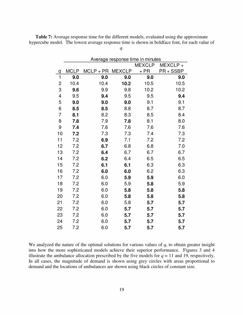
Table 7: Average response time for the different models, evaluated using the approximate
hypercube model. The lowest average response time is shown in boldface font, for each value of
q.
q MCLP MCLP + PR MEXCLP
MEXCLP
+ PR
MEXCLP +
PR + SSBP
1 9.0 9.0 9.0 9.0 9.0
2 10.4 10.4 10.2 10.5 10.5
3 9.6 9.9 9.8 10.2 10.2
4 9.5 9.4 9.5 9.5 9.4
5 9.0 9.0 9.0 9.1 9.1
6 8.5 8.5 8.8 8.7 8.7
7 8.1 8.2 8.3 8.5 8.4
8 7.8 7.9 7.8 8.1 8.0
9 7.4 7.6 7.6 7.6 7.6
10 7.2 7.3 7.3 7.4 7.3
11 7.2 6.9 7.1 7.2 7.2
12 7.2 6.7 6.8 6.8 7.0
13 7.2 6.4 6.7 6.7 6.7
14 7.2 6.2 6.4 6.5 6.5
15 7.2 6.1 6.1 6.3 6.3
16 7.2 6.0 6.0 6.2 6.3
17 7.2 6.0 5.9 5.9 6.0
18 7.2 6.0 5.9 5.8 5.9
19 7.2 6.0 5.8 5.8 5.8
20 7.2 6.0 5.8 5.8 5.8
21 7.2 6.0 5.8 5.7 5.7
22 7.2 6.0 5.7 5.7 5.7
23 7.2 6.0 5.7 5.7 5.7
24 7.2 6.0 5.7 5.7 5.7
25 7.2 6.0 5.7 5.7 5.7
Average response time in minutes
We analyzed the nature of the optimal solutions for various values of q, to obtain greater insight
into how the more sophisticated models achieve their superior performance. Figures 3 and 4
illustrate the ambulance allocation prescribed by the five models for q = 11 and 19, respectively.
In all cases, the magnitude of demand is shown using grey circles with areas proportional to
demand and the locations of ambulances are shown using black circles of constant size.
20
MCLP
MEXCLP
MCLP+PR
MEXCLP+PR
MEXCLP+PR+SSBP
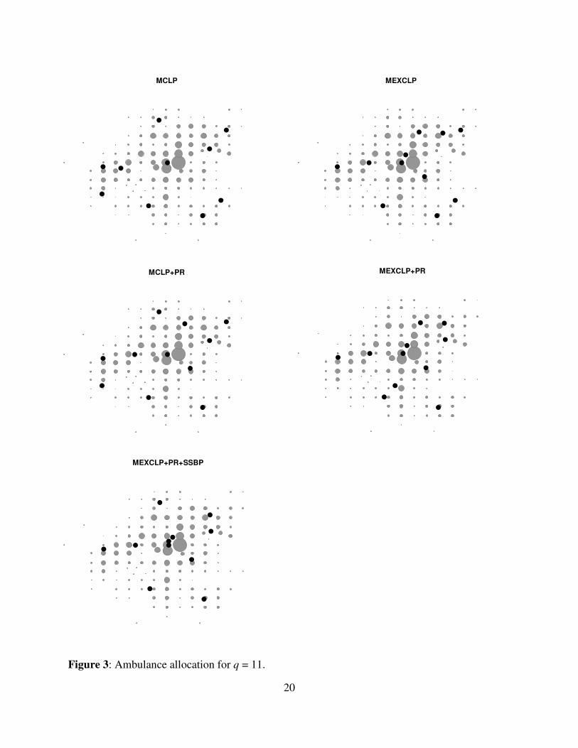
Figure 3: Ambulance allocation for q = 11.
21
With 11 ambulances to be allocated to 16 stations (Figure 3), MCLP uses only 10 stations,
because this achieves the maximum possible coverage, under the assumptions of that model.
The MCLP+PR is qualitatively similar in that it spreads the ambulances throughout the city
relatively evenly. The difference is that this model uses all 11 available ambulances. The
MEXCLP and MEXCLP+PR solutions locate two ambulances in close proximity to each other
near the city center, where most of the demand is concentrated. MEXCLP+PR+SSBP
concentrates the ambulances even more strongly near the city centre, with two ambulances at one
central station and one at the other.
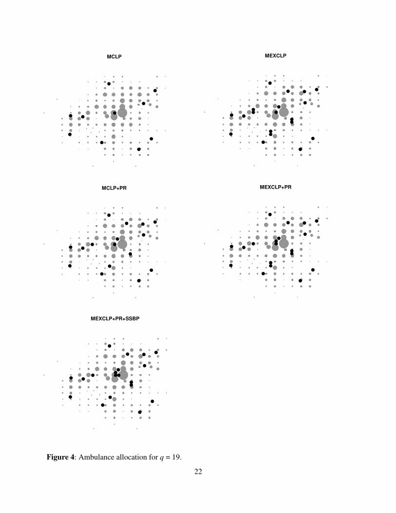
With 19 available ambulances (Figure 4), the MCLP solution remains the same—using only 10
ambulances. MCLP+PR uses all 16 stations, but realizes no benefit from “doubling up” at any
of the stations, because it ignores ambulance availability. MEXCLP doubles up at three stations,
but none of those stations are in the city center. MEXCLP+PR also doubles up at three stations,
one of them in the city centre. MEXCLP+PR+SSBP allocates three ambulances to the most
central station and two ambulances to another station close to the city center. Discussions with
EMS practitioners in Edmonton suggest that they would always double up at the most centrally
located stations before doubling up at outlying stations. Thus, the solutions to MEXCLP+PR
and MEXCLP+PR+SSBP are likely to be more acceptable to them than the solution to
MEXCLP.
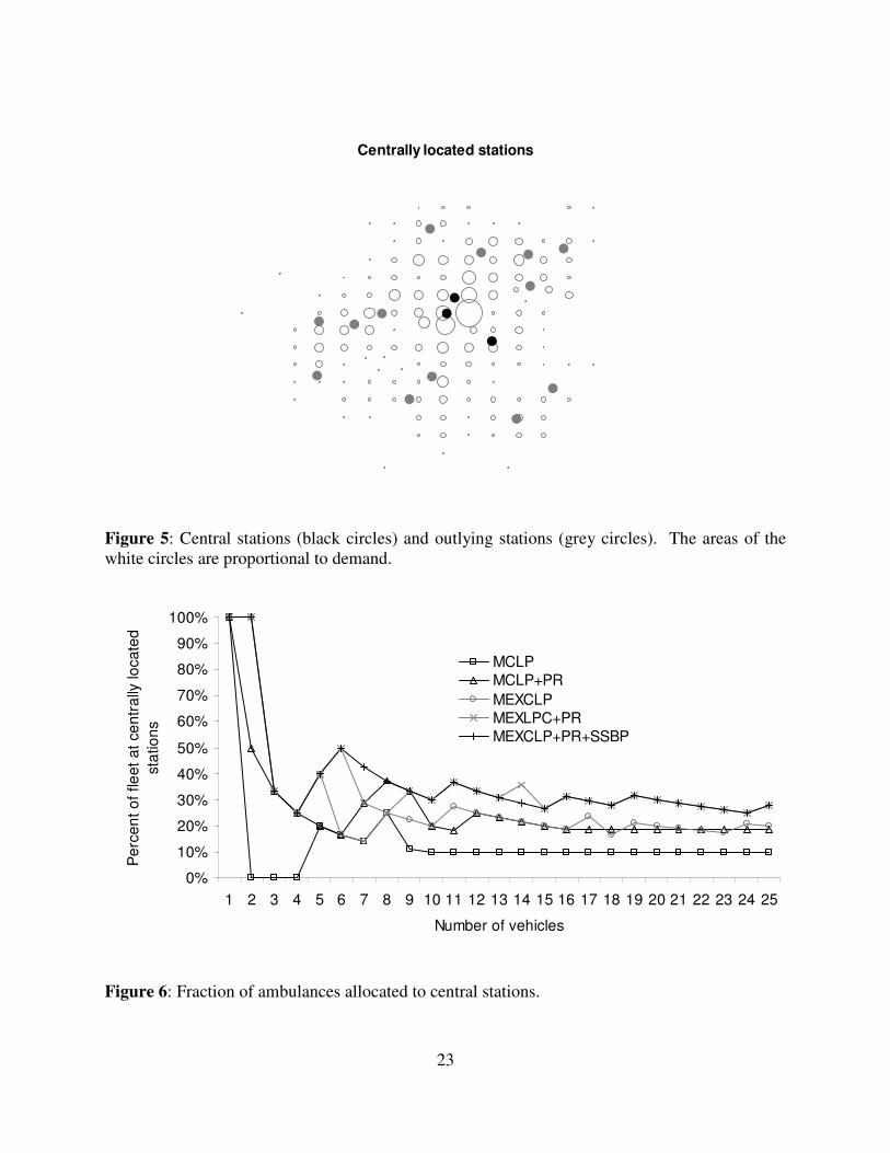
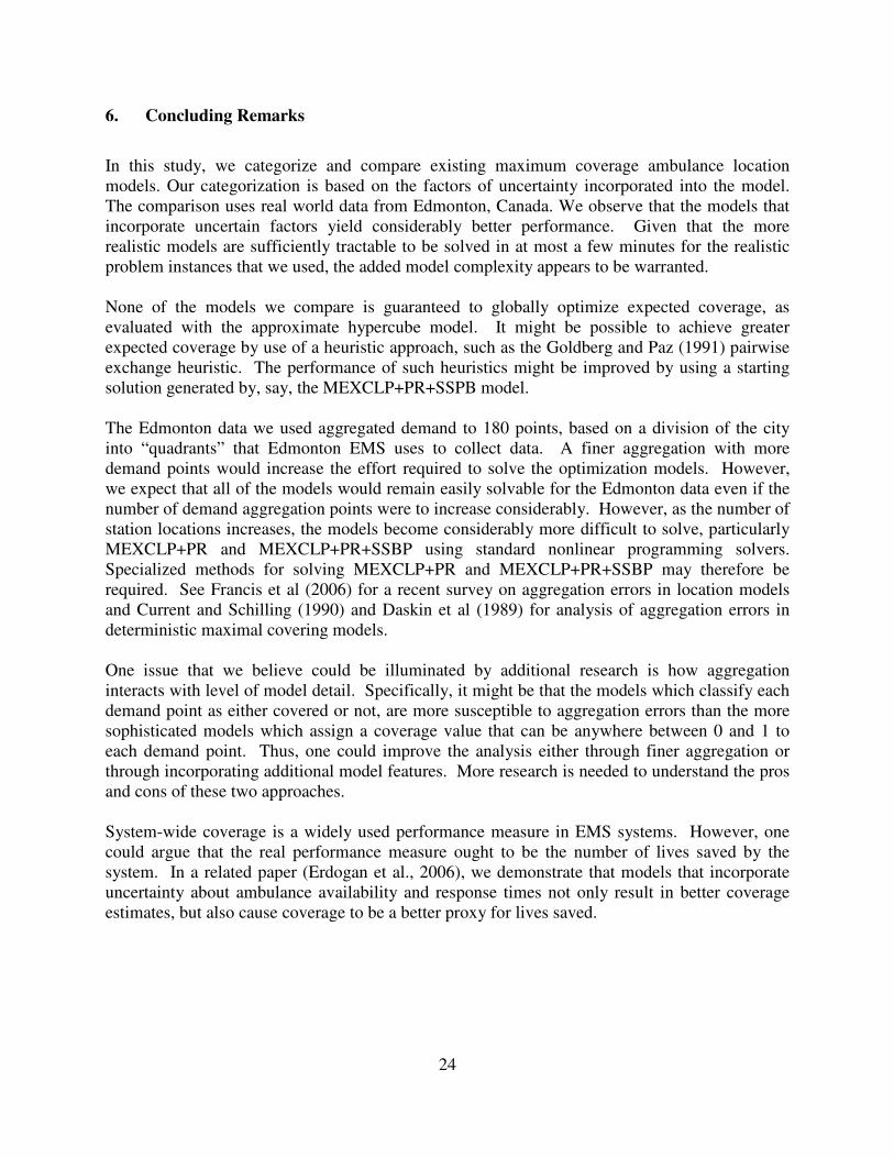
Next, we designated three of the 16 stations (shown with black circles in Figure 5) as central and
the other thirteen as outlying (grey circles), and we computed the fraction of the ambulance fleet
that was allocated to central stations for each model. The results are shown in Figure 6. MCLP
settles down at around 10%, MCLP+PR and MEXCLP at around 20%, and MEXCLP+PR and
MEXLCP+PR+SSBP at around 30%. The last figure corresponds roughly to the fraction of the
total demand that occurs near the city center. We see from this that the improved expected
coverage of the MEXCLP+PR and MEXCLP+PR+SSBP models is achieved through
concentration of resources in areas where demand is highest so as to serve this demand with high
probability.
22
MCLP
MEXCLP
MCLP+PR
MEXCLP+PR
MEXCLP+PR+SSBP
Figure 4: Ambulance allocation for q = 19.
23
Centrally located stations
Figure 5: Central stations (black circles) and outlying stations (grey circles). The areas of the
white circles are proportional to demand.
0%
10%
20%
30%
40%
50%
60%
70%
80%
90%
100%
1 2 3 4 5 6 7 8 9 10 11 12 13 14 15 16 17 18 19 20 21 22 23 24 25
Number of vehicles
Pe
rce
nt
of
fle
et
at
ce
ntr
ally
lo
ca
ted
sta
tio
ns
MCLP
MCLP+PR
MEXCLP
MEXLPC+PR
MEXCLP+PR+SSBP
Figure 6: Fraction of ambulances allocated to central stations.
24
6. Concluding Remarks
In this study, we categorize and compare existing maximum coverage ambulance location
models. Our categorization is based on the factors of uncertainty incorporated into the model.
The comparison uses real world data from Edmonton, Canada. We observe that the models that
incorporate uncertain factors yield considerably better performance. Given that the more
realistic models are sufficiently tractable to be solved in at most a few minutes for the realistic
problem instances that we used, the added model complexity appears to be warranted.
None of the models we compare is guaranteed to globally optimize expected coverage, as
evaluated with the approximate hypercube model. It might be possible to achieve greater
expected coverage by use of a heuristic approach, such as the Goldberg and Paz (1991) pairwise
exchange heuristic. The performance of such heuristics might be improved by using a starting
solution generated by, say, the MEXCLP+PR+SSPB model.
The Edmonton data we used aggregated demand to 180 points, based on a division of the city
into “quadrants” that Edmonton EMS uses to collect data. A finer aggregation with more
demand points would increase the effort required to solve the optimization models. However,
we expect that all of the models would remain easily solvable for the Edmonton data even if the
number of demand aggregation points were to increase considerably. However, as the number of
station locations increases, the models become considerably more difficult to solve, particularly
MEXCLP+PR and MEXCLP+PR+SSBP using standard nonlinear programming solvers.
Specialized methods for solving MEXCLP+PR and MEXCLP+PR+SSBP may therefore be
required. See Francis et al (2006) for a recent survey on aggregation errors in location models
and Current and Schilling (1990) and Daskin et al (1989) for analysis of aggregation errors in
deterministic maximal covering models.
One issue that we believe could be illuminated by additional research is how aggregation
interacts with level of model detail. Specifically, it might be that the models which classify each
demand point as either covered or not, are more susceptible to aggregation errors than the more
sophisticated models which assign a coverage value that can be anywhere between 0 and 1 to
each demand point. Thus, one could improve the analysis either through finer aggregation or
through incorporating additional model features. More research is needed to understand the pros
and cons of these two approaches.
System-wide coverage is a widely used performance measure in EMS systems. However, one
could argue that the real performance measure ought to be the number of lives saved by the
system. In a related paper (Erdogan et al., 2006), we demonstrate that models that incorporate
uncertainty about ambulance availability and response times not only result in better coverage
estimates, but also cause coverage to be a better proxy for lives saved.

25
References
Borras, F., J. T. Pastor. (2002). “The Ex-Post Evaluation of the Minimum Local Reliability
Level: An Enhanced Probabilistic Location Set Covering Model.” Annals of Operations
Research 111, 51-74.
Borras, F., J. T. Pastor. (2003). “The Binomial Probabilistic Location Set Covering Problem:
Revisited.” Working paper.
Brotcorne, L., G. Laporte, F. Semet. (2003). “Ambulance Location and Relocation Models.”
European Journal of Operational Research 147, 451-463.
Budge, S., A. Ingolfsson, E. Erkut. (2005). “Approximating Vehicle Dispatch Probabilities for
Emergency Service Systems.” Working paper, available from
http://www.business.ualberta.ca/aingolfsson/working_papers.htm.
Chaiken, J.M., R.C. Larson. (1972). “Methods for Allocating Urban Emergency Units: A
Survey.” Management Science 19, 110-130.
Church, R., C. ReVelle. (1974). “The Maximal Covering Location Problem.” Papers of the
Regional Science Association 32:101-120.
Current, J.R., D.A. Schilling. (1990). “Analysis of Errors Due to Aggregation in Set Covering
and Maximal Covering Models.” Geographical Analysis 22, 116-126.
Daskin, M.S. (1983). “A Maximum Expected Covering Location Model: Formulation,
Properties, and Heuristic Solution.” Transportation Science 17:48-70.
Daskin, M.S. (1987). “Location, Dispatching, and Routing Model for Emergency Services with
Stochastic Travel Times.” In Spatial Analysis and Location Allocation Models, A. Ghosh and
G. Rushton (eds.). Van Nostrang Reinhold Company, New York, 224-265.
Daskin, M.S., A.E. Haghani, M. Khanal, C. Malandraki. (1989). “Aggregation Effects in
Maximum Covering Models.” Annals of Operations Research 18, 115-140.
Eaton, D.J., M.S. Daskin, D. Simmons, B. Bulloch, G. Jansma. (1985). “Determining Emergency
Medical Service Vehicle Deployment in Austin, Texas.” Interfaces 15, 96-108.
Erdoğan, G., E. Erkut, A. Ingolfsson. (2006). “Ambulance Deployment for Maximum Survival.”
Working paper.
Erkut, E., A. Ingolfsson, S. Budge (2006). “Maximum Availability Models for Selecting
Ambulance Station and Vehicle Locations: a Critique.” Working paper.
Fitch, J. (2005). “Response Times: Myths, Measurement & Management.” Journal of
Emergency Medical Services 30, 46-56
Francis, R.L., T.J. Lowe, B. Rayco, A. Tamir. (2005). “Aggregation Error for Location Models:
Survey and Analysis.” Annals of Operations Research, forthcoming.
Goldberg, J., L. Paz. (1991). “Locating Emergency Vehicle Bases when Service Time Depends
on Call Location.” Transportation Science 25, 264–280.
Ingolfsson, A., S. Budge, E. Erkut. (2006). “Optimal Ambulance Location with Random Delays
and Travel Times: Draft 2.” Working paper, available from
http://www.business.ualberta.ca/aingolfsson/working_papers.htm.
Ingolfsson, A., S. Budge, E. Erkut. (2003). “Optimal Ambulance Location with Random Delays
and Travel Times: Draft 1.”
Jarvis, J. (1975). “Optimization in Stochastic Service System with Distinguishable Servers.”
Ph.D. dissertation, Massachusetts Institute of Technology.
Jarvis, J. (1985). “Approximating the Equilibrium Behavior of Multi-Server Loss Systems.”
Management Science 31, 235–239.
26
Larson, R. C. (1975). “Approximating the Performance of Urban Emergency Service Systems.”
Operations Research 23, 845–868.
Marianov, V., C. ReVelle. (1995). “Siting Emergency Services,” in Facility Location: A Survey
of Applications and Methods, Drezner, Z., ed. Springer Series in Operations Research, 199-
222.
Marianov V., C. Revelle. (1996). “The Queueing Maximal Availability Location Problem: a
Model for the Siting of Emergency Vehicles.” European Journal of Operational Research
93, 110-120.
National Fire Protection Association. (2004). NFPA 1710: Standard for the Organization and
Deployment of Fire Suppression Operations, Emergency Medical Operations, and Special
Operations to the Public by Career Fire Departments, NFPA, Quincy, MA.
Revelle, C., K. Hogan. (1989). “The Maximum Availability Location Problem.” Transportation
Science 23, 192-200
Revelle, C., D. Bigman, D. Schilling, J. Cohon, R. Church. (1977). “Facility Location: a Review
of Context-free and EMS models.” Health Services Research 12, 129-146
Saydam, C., M. McKnew. (1985). “A Separable Programming Approach to Expected Coverage:
An Application to Ambulance Location.” Decision Sciences 16, 381-398.
Swersey, A.J. (1994). “The Deployment of Police, Fire, and Emergency Medical Units.” In
Handbooks in Operations Research and Management Science, Vol. 6: Operations Research
and the Public Sector, A. Barnett, S.M. Pollock, and M.H. Rothkopf (eds.). North-Holland.
Toregas, C., R. Swain, C. Revelle, L. Bergman. (1971). “The Location of Emergency Service
Facilities.” Operations Research 19, 1363-1373.
Williams, D. (2005). “2004 JEMS 200 City Survey: a Snapshot of Facts & Trends to Create
Benchmarks for Your Service.” Journal of Emergency Medical Services 30, 42-60.


