

Washington University in St. LouisWashington University Open Scholarship
All Theses and Dissertations (ETDs)
5-24-2012
Composite Multi resolution Analysis WaveletsBenjamin ManningWashington University in St. Louis
Follow this and additional works at: https://openscholarship.wustl.edu/etd
This Dissertation is brought to you for free and open access by Washington University Open Scholarship. It has been accepted for inclusion in AllTheses and Dissertations (ETDs) by an authorized administrator of Washington University Open Scholarship. For more information, please [email protected].
Recommended CitationManning, Benjamin, "Composite Multi resolution Analysis Wavelets" (2012). All Theses and Dissertations (ETDs). 716.https://openscholarship.wustl.edu/etd/716
WASHINGTON UNIVERSITY IN ST. LOUIS
Department of Mathematics
Dissertation Examination Committee:Guido Weiss, Co-Chair
Edward Wilson, Co-ChairBrody Johnson
Joseph O’SullivanNik Weaver
Victor Wickerhauser
Composite Multi resolution Analysis Wavelets
by
Benjamin Manning
A dissertation presented to theGraduate School of Arts and Sciences
of Washington University inpartial fulfillment of the
requirements for the degreeof Doctor of Philosophy
May 2012
Saint Louis, Missouri

Copyright by
Benjamin Manning
2012

Acknowledgements
I am truly grateful to have had two phenomenal advisors Guido Weiss and Edward
Wilson. I am thankful for their patience, knowledge, time, and support throughout
my graduate school experience. I truly appreciate the countless hours they have spent
discussing wavelets with me and guiding me towards completion of my work. I am
thankful for them introducing me to the wavelet community and to the beauty of
their work on wavelets. Without their help, this work would not have been possible.
I would like to thank Nik Weaver who was an excellent teacher and made my first two
years at Washington University the best two years I’ve spent studying mathematics.
I would like to thank Washington University and the Mathematics Department for
financial support over the years from 2007–2012. I am grateful to my friends and
family for their support. I am thankful for my friends Tim, Jeff, and Jasmine who
have made my time at Washington University the most enjoyable period of my life.
ii

Contents
Acknowledgements ii
Chapter 1. Introduction 1
Results 6
Chapter 2. Harmonic Analysis on Crystallographic Groups 11
2.1. Introduction 11
2.2. Translation invariant spaces 11
2.3. Crystallographic groups 14
2.4. Fourier Transform 21
2.5. Fourier Series 24
2.6. Refinable functions 32
2.7. Shift Invariant Spaces 35
Chapter 3. Multi resolution Analysis 58
3.1. Composite MRA 58
3.2. Existence and construction of MRA wavelets 62
3.3. Basic properties of MRA 73
3.4. Constructing MRA scaling functions from M0 85
3.5. Orthogonality of shifts 97
Chapter 4. Accuracy 105
4.1. Introduction 105
4.2. Accuracy 112
iii

4.3. Compactly Supported Composite Wavelets on R. 123
4.4. The Cascade Algorithm 142
4.5. Conclusions 144
Bibliography 146
iv

CHAPTER 1
Introduction
A function ψ ∈ L2(R) is called a wavelet if the collection of functions
2j/2ψ(2j · −k) : j, k ∈ Z,
forms an orthonormal basis for L2(R). The simplest compactly supported wavelet is
the Haar wavelet
ψ = χ[0,1/2) − χ[1/2,1).
The practical applications of wavelets arose out of a specific subclass of wavelets.
This class is called the multi-resolution analysis wavelets. A multi-resolution analysis
(MRA) is a sequence of closed subspaces Vjj∈Z ⊂ L2(Rn) so that
(1) f(2j·) ∈ Vj if and only if f ∈ V0;
(2) Vj ⊂ Vj+1 ;
(3)⋂j∈Z Vj = ∅;
(4)⋃j∈Z Vj = L2(Rn) ;
(5) There exists ϕ ∈ V0 whose integer translates form an orthonormal basis for
V0.
The definition of a MRA may seem strange at first, but their use stems from their
multi-scaled approach to problems. Additionally, any compactly supported wavelet
must arise from a MRA. The function ϕ ∈ V0 in condition v) is called a scaling
function. The scaling function is not unique, but any other scaling function in V0 can
1

readily be obtained from another. To construct a wavelet, we define for all j ∈ Z,
Wj = Vj+1 Vj.
That is, Wj is the orthogonal complement of Vj in Vj+1. It is then possible to find
ψ ∈ W0 so that its translates form an orthonormal basis for W0. This ψ will then
be a wavelet and we will call it a MRA wavelet associated with the MRA Vjj∈Z.
Conditions i), ii), and v) imply that ϕ is refinable. This means there exists ckk∈Z ⊂
l2(Z) such that
(1.0.1) ϕ(x) =∑k∈Z
ckϕ(2x− k),
with convergence in L2(R). The equation above is called the refinement equation and
is central to studying MRA wavelets. The ckk∈Z are called the mask associated
with the refinement equation. Applying the Fourier transform to both sides of the
refinement equation, we can express the equation above as
ϕ(2ξ) = m0(ξ)ϕ(ξ),
where m0(ξ) = 12
∑k∈Z cke
−2πiξk. The function m0 is called the low-pass filter. We
can also define a wavelet ψ ∈ W0 in terms of ϕ. In fact,
ψ(x) =∑k∈Z
(−1)kc1−kϕ(2x− k).
This can be expressed in terms of the Fourier transform as
ψ(2ξ) = m1(ξ)ϕ(ξ),
where m1(ξ) = −e−2πiξm0(ξ + 1/2). The function m1 is called the high-pass filter.
It is worth noting that the scaling function and wavelet can be determined directly
from the refinement mask ckk∈Z. One way to construct the scaling function from
2

the refinement mask is to construct a sequence with elementary initial element by
iteratively applying the operator
T (f) =∑k∈Z
ckf(2x− k).
Under certain constraints, this sequence will converge in distribution to the scaling
function. This process can also be expressed in terms of the Fourier transform,
|ϕ(ξ)|2 =∞∏j=1
|m0(2−jξ)|2.
Under certain constraints, we can remove the absolute value signs and write
ϕ(ξ) =∞∏j=1
m0(2−jξ).
The formula above will hold for any compactly supported scaling function. The most
useful examples of wavelets are constructed by this process. So the question of finding
wavelets is often reduced to finding the appropriate coefficients in the refinement
equation. The properties of MRA wavelets can be characterized by conditions on the
coefficients in the refinement equation.
With this overview of MRA wavelets in mind, we can now describe some of the
basic properties of the Daubechies wavelets. The Daubechies wavelets are smooth,
compactly supported, MRA wavelets with several desirable properties. The first
property is that they are compactly supported and so are their scaling functions. A
scaling function is compactly supported if and only if the refinement mask is finitely
supported. In most applications, the refinement mask is the element used in compu-
tations and neither the scaling function nor the wavelet function are explicitly used.
Having a finitely supported refinement mask is essential for applications. The second
3
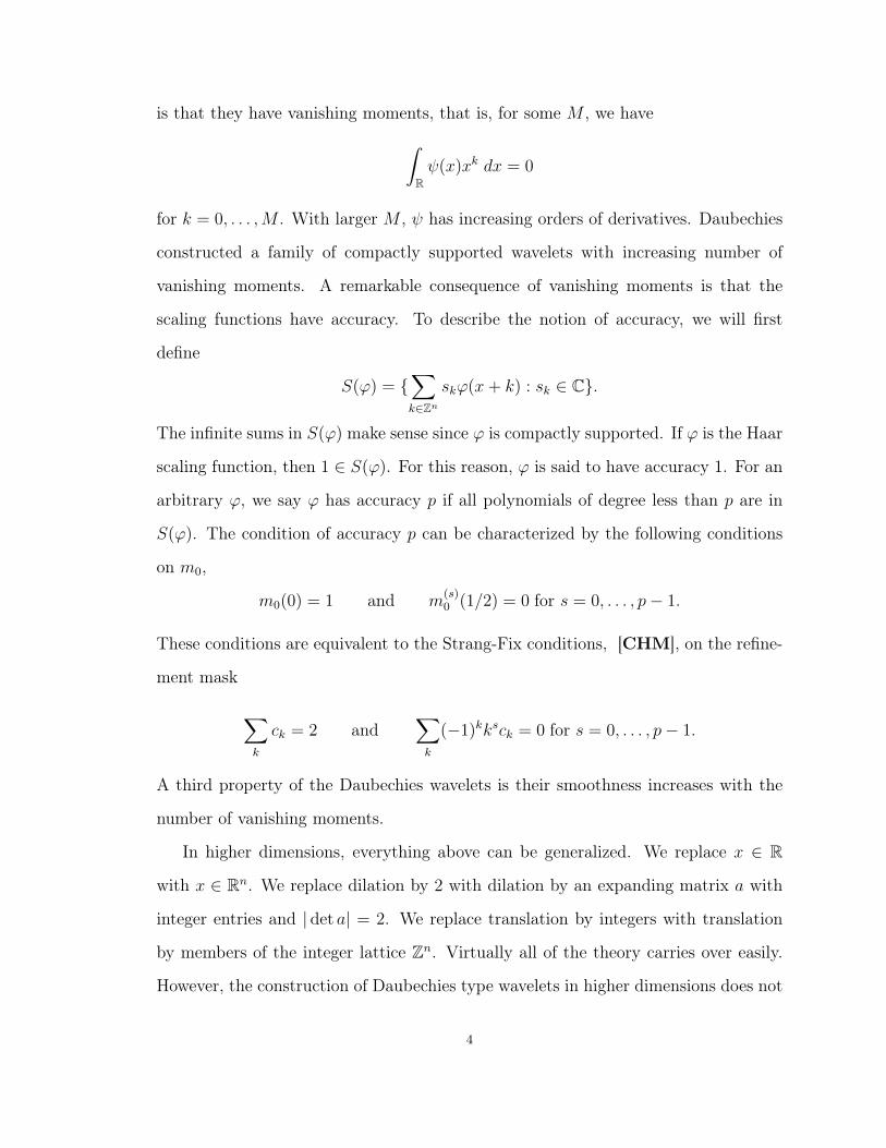
is that they have vanishing moments, that is, for some M , we have
ˆRψ(x)xk dx = 0
for k = 0, . . . ,M . With larger M , ψ has increasing orders of derivatives. Daubechies
constructed a family of compactly supported wavelets with increasing number of
vanishing moments. A remarkable consequence of vanishing moments is that the
scaling functions have accuracy. To describe the notion of accuracy, we will first
define
S(ϕ) = ∑k∈Zn
skϕ(x+ k) : sk ∈ C.
The infinite sums in S(ϕ) make sense since ϕ is compactly supported. If ϕ is the Haar
scaling function, then 1 ∈ S(ϕ). For this reason, ϕ is said to have accuracy 1. For an
arbitrary ϕ, we say ϕ has accuracy p if all polynomials of degree less than p are in
S(ϕ). The condition of accuracy p can be characterized by the following conditions
on m0,
m0(0) = 1 and m(s)0 (1/2) = 0 for s = 0, . . . , p− 1.
These conditions are equivalent to the Strang-Fix conditions, [CHM], on the refine-
ment mask
∑k
ck = 2 and∑k
(−1)kksck = 0 for s = 0, . . . , p− 1.
A third property of the Daubechies wavelets is their smoothness increases with the
number of vanishing moments.
In higher dimensions, everything above can be generalized. We replace x ∈ R
with x ∈ Rn. We replace dilation by 2 with dilation by an expanding matrix a with
integer entries and | det a| = 2. We replace translation by integers with translation
by members of the integer lattice Zn. Virtually all of the theory carries over easily.
However, the construction of Daubechies type wavelets in higher dimensions does not
4

carry over. In the example of the quincunx dilation,
a =
1 −1
1 1
,
Figure 1: Haar scaling function for the quincunx dilation matrix.
there are no known examples of compactly supported differentiable wavelets. Even
the simplest examples, the Haar wavelet associated with a is a simple function
defined on fractal "twin dragon" sets. My advisors thought to introduce an
additional finite subgroup of dilations. For any matrix c ∈ GLn(R) we define the
dilation operator Dc : L2(Rn)→ L2(Rn) as Dc(f)(x) = | det c|−1/2f(c−1x). For any
w ∈ Rn, we define the translation operator Tw : L2(Rn)→ L2(Rn) as
Tw(f)(x) = f(x− w). We fix a dilation matrix a. We let B be a finite subgroup of
SLn(Z) so that aBa−1 = B. We say ψ ∈ L2(Rn) is a composite wavelet if the system
DajDbTkψ : b ∈ B, j ∈ Z, k ∈ Zn
5

forms an orthonormal basis for L2(Rn). There is an analogous definition of a MRA
called the composite MRA. With the addition of these new dilations, Krishtal,
Robinson, Weiss, and Wilson in [KRWW] produced a simple example of a Haar
type composite wavelet that is a simple function on triangles. The support set is a
dramatically simpler set than that of the "twin dragon." This gave strong
motivation to search for Daubechies type composite wavelets and that is the central
goal of this research.
-
+
(1/2,1/2)
(0,0) (1/2,0)
Figure 1: Haar wavelet for the group of eight symmetries of the square. The wavelet is equal to
+√
8 on the light gray area and equal to −√
8 on the dark gray area. This composite wavelet was
constructed in [KRWW].
Results
The dissertation focuses on two parts. One is developing a foundation for com-
posite MRA wavelets similar to what one would find in [HSWW] and [TLW]. The
second is applying these tools to produce examples of Daubechies type composite
MRA wavelets. We will take one slight departure from composite wavelet systems
and require B to be a finite group of isometries on Rn with Zn replaced by a full
6

rank lattice L with BL = L. This will make the semi-direct product Γ = B n L a
crystallographic group. An important feature is that Γ will have a compact funda-
mental domain, which is necessary for us to produce the simplest of wavelets: the
Haar wavelets.
The abelian group of integers Zn is now replaced with a discrete group of isome-
tries Γ. The non-commutativity of this group will often imply replacing commutative
elements with non-commutative elements. For example, the low and high pass fil-
ters above are now matrices. The high pass filter m1 is no longer determined by
a simple formula such as m1(ξ) = e2πiξm0(ξ + 1/2). In some cases it can be diffi-
cult to determine an appropriate formula for m1. The traditional Fourier transform
is now replaced with a vector valued Fourier transform. Much of the traditional
theory of MRA wavelets easily carries over. However, some of it does not and a
large part of this research is overcoming the difficulties of this non-commutativity to
produce results similar to those found in the traditional case. For any γ ∈ Γ, we
define Lγ : L2(Rn) → L2(Rn) as Lγ(f)(x) = f(γ−1(x)). We fix an expanding matrix
a ∈ GLn(R) so that aΓa−1 ⊂ Γ. We say ψ ∈ L2(Rn) is an (a,Γ)-wavelet if the system
DajLγψ : j ∈ Z, γ ∈ Γ
forms an orthonormal basis for L2(Rn). We thus define a more general form of a
MRA. An (a,Γ)-MRA is a sequence of closed subspace Vjj∈Z ⊂ L2(Rn) so that
(1) f(aj·) ∈ Vj if and only if f ∈ V0;
(2) Vj ⊂ Vj+1 ;
(3)⋂j∈Z Vj = ∅;
(4)⋃j∈Z Vj = L2(Rn) ;
(5) There exists ϕ ∈ V0 so that Lγϕ : γ ∈ Γ forms an orthonormal basis for
V0.
7

The refinement equation, in this case, becomes
ϕ(x) =∑γ∈Γ
cγϕ(γ(ax)).
In Chapter 2, we will establish a foundation for studying composite wavelets. We
will develop an appropriate Fourier transform and generalize the notion of a Fourier
series to fit our needs for studying composite wavelets. In particular, we will focus
on Γ-invariant subspaces. A Γ-invariant subspace is a closed subspace V of L2(Rn)
so that LγV ⊂ V for all γ ∈ Γ. Much of the theory established in Chapter 2 is
a rather straightforward generalization of the theory of translation invariant spaces.
For example, we establish the basic results concerning frames and generalize notions
such as the bracket and dimension function. Next, a decomposition of Γ-invariant
spaces is established, generalizing the decomposition found in [Bow]. This results
not only confirms that the correct notion of a dimension function has been found,
but also guarantees that, if we have an (a,Γ)-MRA, then there will always exist
(a,Γ)-wavelets associated with that MRA.
In Chapter 3, we will generalize much of traditional MRA theory. We will establish
that when | det a| = 2, there always exists an (a,Γ)-MRA wavelet. When | det a| > 2,
there only exist (a,Γ)-MRA multi-wavelets and we will not pursue these type of
wavelets. A particularly useful result in Chapter 3 is the generalization of the infinite
product
|ϕ(ξ)|2 =∞∏j=1
|m0(2−jξ)|2
to an infinite product of matrices. For any (a,Γ)-MRA, we will prove that a very useful
infinite matrix product formula holds.This formula is analogous to the scalar formula
above and no similar infinite product formula has been found by other investigators.
In the traditional theory of wavelets, there are two well known methods for verifying
the orthogonality of the translates of the scaling function. Both are conditions on
8

the low-pass filter m0. They are called Cohen’s condition and Lawton’s condition
[TLW]. We will establish a variant of the Cohen’s condition for determining the
orthogonality of the system Lγϕ : γ ∈ Γ. In practice, a simple generalization
of Lawton’s condition wins out and we prove a necessary and sufficient verifiable
condition for determining if the system Lγϕ : γ ∈ Γ is orthonormal. We then apply
this result to show various examples of (a,Γ)-MRA wavelets. We also prove, even in
the case when the system Lγϕ : γ ∈ Γ is not orthonormal, the associated wavelet
system DajLγψ : j ∈ Z, γ ∈ Γ forms a normalized tight frame for L2(Rn).
In Chapter 4, we will produce the accuracy equations. These are the generalization
of the Strang-Fix equations. Cabrelli, Heil, and Molter have produced accuracy
equations for multi-generated refinable functions with integer translates. The problem
of determining accuracy for multi-generated refinable functions with integer translates
is inherently complex. We will simply rework their results for a single-generated
refinable function with shifts in Γ to yield comparatively simple accuracy equations.
This gives verifiable conditions to determine the accuracy of a scaling function.
Although the decomposition of shift-invariant spaces in Chapter 2 guarantees that
a high-pass filter always exists, it does not guarantee that the coefficients of the high-
pass filter are finitely supported, which is necessary to ensure the wavelet is also
compactly supported. So we have to determine a specific choice of high-pass filter,
which becomes an algebraic problem. We will succeed in many cases and determine a
structure of the low-pass filters and produce a method for constructing an appropriate
high-pass filter. Then we will use this along with all the previous work to produce
several examples of Daubechies type (a,Γ)-wavelets with various degrees of accuracy.
Even though we have established and provided a solid foundation for studying
composite wavelets, there is much work to be done along with many open questions.
For example, in Chapter 4, we characterize low-pass filters for the simplest of com-
posite wavelets. We also provide a suitable construction for the high-pass filter. Some
9

similar statement for all composite groups would be very helpful in constructing more
examples of composite MRA wavelets. Also, it would be useful to develop a theory
for determining the smoothness of these composite wavelets. This has been done
in the traditional case, [CH], by making use of the joint-spectral radius of multiple
operators. A promising approach would be to generalize this method to composite
wavelets. Also, our examples in Chapter 4 were obtained by solving several qua-
dratic equations with multiple variables. When we search for scaling functions with
higher order accuracy, this quickly becomes a computationally intractable problem.
Anything to simplify this approach would be useful.
10

CHAPTER 2
Harmonic Analysis on Crystallographic Groups
2.1. Introduction
One of the principal tools used in wavelet theory is the Fourier transform on Rn
and Zn. For the classical wavelets, we consider a function f ∈ L2(Rn) and study the
shift invariant space generated by f under the shifts of the discrete group Zn, which
sits inside Rn. If we study shift invariants spaces of L2(Rn), we consider harmonic
analysis on both Rn and Zn. For the composite wavelets, we will be considering
functions f ∈ L2(Rn) with shifts by a crystallographic group Γ, which is a discrete
and often non-abelian group. So just as harmonic analysis on Zn plays a key role
in standard wavelet theory, to develop similar theorems we should establish a basic
theory of harmonic analysis on the group Γ.
The Fourier transform on crystallographic groups was developed by Keith F. Tay-
lor in [Tay]. We rephrase it in a slightly different form, and establish basic and useful
results. We will then establish the basic results of spaces invariant under crystallo-
graphic shifts.
2.2. Translation invariant spaces
We will first review facts about translation invariant spaces. Many of these results
are well known. For example, see [HSWW] and [HSWW2]. We will not provide
any proofs in this section. Let f ∈ L1(Rn), we define the Euclidean Fourier transform
of f , denoted by f , to be
f(ξ) =
ˆRnf(x)e−2πiξ·x dx.
11

Here Rn is the Pontryagin dual of Rn. The mapping Rn → Rn given by ξ 7→ e2πiξ·x is
a continuous isomorphism. It is well known that the Fourier transform extends to a
unitary operator from L2(Rn) onto L2(Rn). Given k ∈ Zn, we define the translation
operator Tk : L2(Rn) → L2(Rn) as Tkf(x) = f(x − k). Recall that the dual group
of Zn is Tn. The lattice dual of Zn, denoted (Zn)∗, is the set of l ∈ Rn such that
e2πil·k = 1 for all k ∈ Zn. In this case, (Zn)∗ is isomorphic to Zn.
For any k ∈ Zn, we define the modulation operator Mk : L2(Rn) → L2(Rn) as
Mkf(ξ) = e2πiξ·kf(ξ). A straightforward calculation shows for any f ∈ L2(Rn),
(T−kf)ˆ = Mkf .
Now, let V be a closed subspace of L2(Rn). We say V is translation invariant if TkV ⊂
V for all k ∈ Zn. Given a f ∈ L2(Rn), we let 〈f〉 denote the smallest translation
invariant subspace generated by f . If g =∑
k∈Zn ckTkf with convergence in L2(Rn),
then applying the Fourier transform to both sides yields g =∑
k∈Zn ckM−kf . If we
let m(ξ) =∑
k∈Zn cke−2πiξ·k, then g = mf . A basic fact is that
〈f〉 = f ∈ L2(Rn) : mf ∈ L2(Rn) m is a 1-periodic measurable function on Rn.
When studying wavelets, we will be interested in translation invariant spaces. We are
interested when Tkfk∈Zn forms a type of basis. In particular, we will be interested
when Tkfk∈Zn forms an orthonormal basis or possibly a frame. We say Tkfk∈Zn
forms a frame if for some A,B > 0 and all g ∈ 〈f〉 we have
A ||g||22 ≤∑k∈Zn|〈g, Tkf〉|2 ≤ B ||g||22 .
12

When A = B = 1, we say Tkfk∈Zn forms a Parseval frame. For f, g ∈ L2(Rn), we
define the bracket of fwith g, denoted by [f , g], as
[f , g](ξ) =∑
k∈(Zn)∗
f(ξ + k)g(ξ + k).
The convergence holds for almost all ξ ∈ Rn. Furthermore, [f , g] ∈ L2(Tn). The
bracket proves to be an invaluable tool for studying shift invariant spaces. We can use
the bracket function to characterize properties of Tkfk∈Zn . For example, Tkfk∈Zn
forms an orthonormal basis if and only if [f , f ](ξ) = 1 for almost all ξ ∈ Tn. Let Ωf
denote the support of [f,f ]. It is also well known that Tkfk∈Zn forms a frame for
〈f〉 with frame constants A,B > 0 if and only if
AχΩf (ξ) ≤ [f,f ](ξ) ≤ BχΩf (ξ)
for almost all ξ ∈ Tn.
Let fii∈N be a subset of L2(Rn). We say Tkfik∈Zn,i∈N forms a Parseval frame
for a translation invariant space V if V = spanTkfik∈Zn,i∈N and if for all g ∈ V we
have
||g||22 =∑
k∈Zn,i∈N
|〈g, Tkfi〉|2 .
If Tkfik∈Zn,i∈N forms a Parseval frame for a translation invariant space V , then we
define the dimension function on V , denoted as dimV , as
dimV (ξ) =∑i∈N
[fi, fi](ξ)
where ξ ∈ Tn. The dimension function is non-negative and at certain points may
equal +∞. The dimension function is well defined and independent of the choice
for fii∈N. If f ∈ L2(Rn) is such that Tkfk∈Zn forms an orthonormal basis for
V = 〈f〉, then dimV (ξ) = 1 for almost all ξ ∈ Tn. A natural question to ask is if the
13

converse is true. That is, if V is a translation invariant space and dimV = 1, does
there exist f ∈ V such that Tkfk∈Zn forms an orthonormal for V ? The answer is
in the affirmative and is a consequence of the following theorem that can be found in
[Bow]:
Theorem 1. Let V be a translation invariant subspace of L2(Rn). Then there
exists a sequence fll∈N such that [fl, fl] = χΩfl, 〈fl〉 ⊥ 〈fm〉 for l 6= m, and V =⊕
l∈N〈fl〉. Furthermore, Ωfl+1⊂ Ωfl for all l ∈ N.
Many of these facts are well known and have been established for some time. In
this chapter, we will replace Zn with discrete group of isometries on Rn, say Γ. These
notions have been generalized to LCA groups in [HSWW2]. We will generalize the
notions of the bracket, dimension function, frames, and Theorem 1 for a discrete non-
Abelian group Γ. It will provide a foundation for studying composite MRA systems.
2.3. Crystallographic groups
We will let Rn be the n×1 column vectors with entries in R. We will now introduce
the group of shifts. The group of isometries of Rn are of the form w 7→ bw+ y where
b is an orthogonal operator on Rn and y ∈ Rn. Let I denote the group of isometries
on Rn and give I the topology of compact convergence. With this topology, I is a
topological group. For each x ∈ Rn we can define a translation map tx : Rn → Rn
given by tx(w) = w − x. The map x 7→ tx is a topological group isomorphism of Rn
with the group of translations in I. For this reason, we may identify each element
in Rn as an element in the group of translations in I. We first establish some basic
results.
Proposition 2. Let b, c be orthogonal transformations on Rn and z, w ∈ Rn.
Then
14
(1) tztw = tz+w
(2) t−1z = t−z
(3) btzb−1 = tbz
(4) btzctw = bctw+c−1z
(5) (btz)−1 = b−1t−bz.
Proof. The first two are clear. As for the third,
btzb−1(x) = btz(b
−1x) = b(b−1x− z) = x− bz = tbz(x).
For the fourth relation,
btzctw(x) = btzc(x− w)
= btz(cx− cw)
= b(cx− cw − z)
= bcx− bcw − bcc−1z
= bctw+c−1z(x).
Now, using the fourth relation, we have
btzb−1t−bz = bb−1t−bz+bz = et0 = e.
Given a subgroup L ⊂ Rn, we can define a group of translations TL = tk : k ∈ L.
Abusing notation, we will often write L instead of TL. The context of our discussion
will determine whether we ought to think of L as a subgroup of Rn or as a subgroup
of I.
15

Definition 3. Let Γ be a discrete subgroup of the isometries on Rn. A full rank
lattice L is a subgroup of Rn so that L = cZn where c ∈ GLn(R). If Γ contains a
full rank lattice TL as a normal subgroup so that Γ/TL is finite, then Γ is called a
crystallographic group.
We will now abandon the notation TL and always write L. For any bta ∈ Γ and
tl ∈ L, we have
btatl(bta)−1 = bta+l−ab
−1 = btlb−1 = tbl.
Thus L is a normal subgroup of Γ if and only if Γ(L) ⊂ L. For any bta ∈ Γ, we define
π : Γ→ I as
π(bta) = b.
Notice,
π(btacta′) = π(bcta′+c−1a) = bc = π(bta)π(cta′).
Thus π is group homomorphism. The image of π, say B, is called the point group of
Γ. Also, observe that kerπ = L and thus Γ/L ∼= B. We say that the crystallographic
group Γ splits if Γ = BL. We will assume throughout the remainder of this
thesis that the crystallographic group splits. Although such an assumption
is not necessary to obtain our results, we have two good reasons for making this
assumption. The first reason is that it dramatically simplifies our calculations and lets
us take a concrete perspective of harmonic analysis on Γ. The second is that all of our
examples are obtained for groups that split. Introducing an added layer of complexity
by analyzing a general crystallographic group seems unnecessary. However, at the end
of this chapter we will provide appropriate generalizations of definitions for this theory
to be generalized to any crystallographic group.
Definition 4. Let G be a subgroup of I and K ⊂ Rn be a set such that∑g∈G χgK = 1. Then we say K is a fundamental region for G.
16

The existences of a compact fundamental region for Γ is not only essential for
our analysis but also for the existence of the simplest of compact wavelets: the Haar
wavelets.
Proposition 5. There exists a compact fundamental region F for Γ such that if
we let P =⋃b∈B bF , then P is a compact fundamental region for L and contains a
neighborhood of the origin.
Proof. Let c ∈ Rn be such that γc 6= c for any γ ∈ Γ with γ 6= 1. Such a c
always exists. Indeed, for each γ ∈ Γ, the set x ∈ Rn : γx = x has measure zero
and thus so does its union over all γ ∈ Γ. Now, we let Fc = x ∈ Rn : ||x− c|| ≤
||γx− c|| for allγ ∈ Γ . We must first show Fc is compact. Since c ∈ GLn(R), then
there exists a1,a2 > 0 so that
a1 ||x|| ≤ ||cx|| ≤ a2 ||x|| .
Let x ∈ Fc and z = c−1x− c−1c , then for all k ∈ Zn we have ||x− c|| ≤ ||x− c− ck||.
Thus for all k ∈ Zn we have
a1 ||z|| ≤ a2 ||z − k|| .
For any sequence xl ∈ Fc we let zl = c−1xl − c−1c. So there exists kl ∈ Zn such that
zl − kl ∈ [0, 1)n. Hence
||zl|| ≤a2
a1
||zl − kl|| ≤a2
a1
√n.
Hence there exists a convergence subsequence of zl and thus one for xl. Thus Fc
is compact.
For x ∈ Rn, γxγ∈Γ is a discrete set. Thus there is a minimum distance between
this set and Fc. Let y = γ0x be the element of γxγ∈Γ so that this minimum
17

is obtained. Then it is true that ||γ0x− c|| ≤ ||γγ0x− c|| for all γ ∈ Γ. Hence
x ∈ γ−10 Fc ⊂
⋃γ∈Γ γFc . We conclude Rn =
⋃γ∈Γ γFc .
Now, let x ∈ Rn be such that for some γ0 ∈ Γ we have x ∈ Fc∩γ0Fc. This implies∣∣∣∣γ−10 x− c
∣∣∣∣ = ||x− c|| =∣∣∣∣γ−1
0 x− γ−10 c∣∣∣∣. The points c and γ−1
0 c are distinct and the
set of points that are equidistant from them forms a hyperplane in Rn, which has
measure zero. Hence |Fc ∩ γ0Fc| = 0. Therefore∑
γ∈Γ χγFc = 1.
Next, define Pc =⋃b∈B bFc. Let S = bcb∈B. We show Pc = x ∈ Rn : ||x− S|| ≤
||x− k − S|| for all k ∈ L. Let x ∈ Pc, then for some b ∈ B we have b−1x ∈ Fc. Thus
for all γ ∈ Γ,
||x− S|| ≤∣∣∣∣b−1x− c
∣∣∣∣ ≤ ∣∣∣∣γb−1x− c∣∣∣∣ .
This implies ||x− S|| ≤ ||x− k − S|| for all k ∈ L. Conversely, suppose x ∈ Rn and
||x− S|| ≤ ||x− k − S|| for all k ∈ L. Now, there exists b ∈ B such that ||b−1x− c|| =
||x− S||. Thus for all d ∈ B we have ||b−1x− c|| ≤ ||x− k − d−1c|| = ||d(x− k)− c||
. This implies x ∈ bFc and so x ∈ Pc. We can conclude that Pc = x ∈ Rn :
||x− c|| ≤ ||x− k − c|| for all k ∈ L. Since c + k 6= c for any k ∈ L with k 6= 0,
then we can apply our earlier result with the case Γ = L to conclude that Pc is a
compact fundamental region for L. Now let ε = mink∈L−0 ||k||. If c ∈ B(0, ε/4) and
x ∈ B(0, ||c||), then
||x− k − c|| ≥ ||k|| − ||x|| − ||c|| ≥ ε− ε/4− ε/4 = ε/2 ≥ ||x− c|| .
Hence B(0, ||c||) ⊂ Pc. We pick c ∈ B(0, ε/4) and let P = Pc. Then P has the desired
properties.
Typically we will make arguments where we write two sets as being equal except
for a set of measure zero. For example, given a fundamental domain F , we will write⋃γ∈Γ γF = Rn. These two sets may not be equal, only equal except for a set of
measure zero. We will not develop a notation to distinguish between set theoretic
18

equality and measure theoretic equality. Throughout this thesis, we will always as-
sume measure theoretic equality. We will let Σ(F ) = x ∈ Rn :∑
γ∈Γ χγF (x) = 1.
The statement that F forms a fundamental domain for Rn is equivalent to the state-
ment that Rn − Σ(F ) has measure zero. Also, if we let P =⋃d∈B dF , then for all
x ∈ Σ(F ) we have∑
k∈L χP (x+ k) = 1. Sometimes we will want to argue that a set
S is contained in T except on a set of measure zero by arguing that, if x ∈ S, then
x ∈ T for all x ∈ Σ(F ). Whenever a fundamental domain is specified and we make a
statement about set inclusion or equality, we mean that it holds for all x ∈ Σ(F ).
We will denote elements in Rn with letters of the Roman alphabet, say x, y, z, and
elements of its dual Rn with letters of the Greek alphabet, say ξ, η. We will let Rn be
the set of 1×n row vectors with entries in R. We can define an isomorphism between
Rn and the Pontryagin dual of Rn by the mapping ξ 7→ eξ where eξ(x) = e2πiξ·x for
x ∈ Rn. The notation ξ · x simply means the ordinary matrix product of ξ with x or
equivalently the dot product of ξ with x. Given a matrix b from Rn to Rn, we can
multiply an element ξ ∈ Rn on the right by b. That is, we will write ξb, which makes
sense because ξ is a 1× n row vector. We will now define a dual of Γ, denoted by Γ∗.
Recall, the dual lattice, denoted L∗, is the set of k ∈ Rn such that e2πik·l = 1 for all
l ∈ L. A simple calculation shows L∗ = (Zn)∗c−1 where Zn∗ is the set of 1×n vectors
with entries in Z. Since every b ∈ B is an orthogonal matrix, then bt = b−1 ∈ B.
Now, for all k ∈ Zn and b ∈ B we have c−1bck ∈ Zn. Thus ktctbtc−t ∈ Zn for all
k ∈ Zn and b ∈ B. Hence (L∗)B ⊂ L∗. We define Γ∗ = L∗B = BL∗, then Γ∗ is a
crystallographic group. Throughout this chapter, we will fix a fundamental
domain F for Γ∗ and P for L∗ as constructed in Proposition 5.
We now create our fundamental building block for our analysis on Γ. We endow
B with the counting measure. For each ξ ∈ Rn and btx ∈ Γ, we define the operator
19

U ξbtx
: L2(B)→ L2(B) as
U ξbtx
(F )(s) = e2πiξ·(s−1bx)F (b−1s).
For any Hilbert space V , we let B(V ) denote the set of bounded operators on V . For
any γ ∈ Γ we define the mapping Uγ : Rn → B(L2(B)) as ξ 7→ U ξγ . The operator U ξ
γ
is the analogue of e2πiξ·x. When we generalize classical wavelet theory, we will often
be replacing e2πiξ·x with U ξγ .
Proposition 6. The mapping g 7→ U ξg for g ∈ I is a unitary representation on
I.
Proof. For any orthogonal matrices b, c and x, y ∈ Rn, we have
U ξbtxU ξcty(F )(s) = e2πiξ·s−1bxU ξ
cty(F )(b−1s)
= e2πiξs−1b·xe2πiξ·s−1bcyF (c−1b−1s)
= e2πiξ·s−1bc(c−1x+y)F ((bc)−1s)
= U ξbcty+c−1x
(F )(s)
= U ξbtxcty
(F )(s).
Thus the mapping g 7→ U ξg is a group homomorphism. Since
∑s∈B
|U ξbtx
(F )(s)|2 =∑s∈B
|F (sb)|2 =∑s∈B
|F (s)|2,
then U ξbtx
is unitary.
The representation above is the representation induced by the representation x 7→
e2πiξ·x. The matrices U ξγ have a certain symmetry. For any c ∈ B we define Rc :
l2(B)→ l2(B) as Rcf(x) = f(xc). It is immediate that Rc are unitary operators.
Proposition 7. We have RcUξγRc−1 = U ξc−1
γ where c ∈ B, γ ∈ Γ, and ξ ∈ Rn.
20

Proof. Let γ = btx. We have
RcUξbtxRc−1F (s) = U ξ
btxRc−1F (sc)
= e2πiξ·(c−1s−1b)xRc−1F (b−1sc)
= e2πiξc−1·(s−1bx)F (sb)
= U ξc−1
btxF (s).
2.4. Fourier Transform
We define δd ∈ L2(B) as δd(s) = 0 for s 6= d and δd(d) = 1. The collection
δdd∈Bforms an orthonormal basis for l2(B).
Definition 8. For any f ∈ L2(Rn), we define the vector valued Fourier transform
as
F(f)(ξ) =∑d∈B
f(ξd−1)δd.
Evaluating U ξbtx
at δd, we have
U ξbtx
(δd)(s) = e2πiξ·s−1bxδd(b−1s)
= e2πiξ·s−1bxδbd(s)
= e2πiξ·d−1xδbd(s).
Thus U ξbtxδd = e2πiξd−1·xδbd. Next, we define Lg : L2(Rn) → L2(Rn) for any g ∈ I
as Lg(f)(x) = f(g−1(x)). Just as translation corresponds to modulation for the
Euclidean Fourier transform, applying the operator Lg corresponds to multiplying by
Ug for the Fourier transform F .
21

Proposition 9. For any g ∈ G we have F(Lgf) = UgF(f).
Proof. Let g = bty. We have
Lgf(ξ) =
ˆRnf(g−1(x))e−2πiξ·x dx
=
ˆRnf(x)e−2πiξ·g(x) dx
= e2πiξb·yˆRnf(x)e−2πiξb·x dx
= e2πiξb·yf(ξb).
Hence
F(Lgf)(ξ) =∑d∈B
Lgf(ξd−1)δd
=∑d∈B
f(ξd−1b)e2πiξd−1b·yδd
=∑d∈B
f(ξd−1)e2πiξd−1·yδbd
=∑d∈B
f(ξd−1)U ξg (δd) = U ξ
gF(f)(ξ).
For any d ∈ B we define Rd : l2(B)→ l2(B) as RdF (s) = F (sd). We then have:
Proposition 10. We have for all f ∈ L2(Rn), RcF(f)(ξc) = F(f)(ξ) where
c ∈ B and ξ ∈ Rn.
Proof. We have
RcF(f)(ξc) =∑d∈B
f(ξcd−1)δdc−1 =∑d∈B
f(ξd−1)δd = F(f)(ξ).
22

We let
L2B(Rn) = ψ ∈ L2(Rn,C|B|) : Rcψ(ξc) = ψ(ξ) for all c ∈ B.
We endow L2B(Rn) with an inner product
〈f, g〉 =1
|B|
ˆRn〈f(ξ), g(ξ)〉 dξ.
In the equation above, we are using the ordinary inner product on C|B|. Notice we
may rewrite the inner product on L2B(Rn) as
〈f, g〉 =1
|B|
ˆRn
Tr(f(ξ)g(ξ)∗) dξ.
Theorem 11. The Fourier transform is a unitary operator from L2(Rn) onto
L2B(Rn).
Proof. Let f, g ∈ L2(Rn). Then
〈F(f),F(g)〉 =1
|B|∑d∈B
ˆRnf(ξd)g(ξd) dξ =
1
|B|∑d∈B
ˆRnf(ξ)g(ξ) dξ = 〈f , g〉 = 〈f, g〉.
So the mapping f 7→ F(f) is an isometry. We now show it is surjective. Let ψ ∈
L2B(Rn) and define h as h(ξ) = 〈ψ(ξ), δ1〉 and let f be the ordinary inverse Fourier
transform of h. We then have
F(f)(ξ) =∑d∈B
〈ψ(ξd−1), δ1〉δd =∑d∈B
〈Rdψ(ξ), δ1〉δd =∑d∈B
〈ψ(ξ), δd〉δd = ψ(ξ).
Thus this mapping is surjective.
23

2.5. Fourier Series
Here we will define an operator valued Fourier transform on functions on Γ. For
any f ∈ l1(Γ), we define for ξ ∈ P
fΓ(ξ) =∑γ∈Γ
f(γ)U ξγ−1 .
Notice that, if f ∈ l1(Γ), then the series above converges uniformly. Now consider
Fourier series on L. For f ∈ l1(L), the Fourier transform with respect to L is given
by
f(ξ) =∑k∈L
f(k)e−2πiξ·k.
We have L = Tnc−1, where L denotes the dual group of L. We know for some measure
m on Tnc−1 we have the inversion formula,
f(k) =
ˆTnc−1
f(ξ)e2πiξ·k dm(ξ).
The measure m will be a Haar measure and thus a scalar multiple of the Lebesgue
measure dξ. By [Rud], since we have chosen the counting measure on L, then the
inversion formula will hold if and only if we choose m so that m(Tnc−1) = 1. Thus
dm(ξ) = | det c|dξ. So we have
f(k) =
ˆTnc−1
f(ξ)e2πiξ·k |detc|dξ.
Our goal in this section will be to prove analogous theorems for the generalized Fourier
series on Γ.
Proposition 12. We have, for b = 1,
Tr(U ξbtx
) =∑d∈B
e2πix·ξd−1
24
and for b 6= 1,
Tr(U ξbtx
) = 0.
Proof. We have,
Tr(U ξbtx
) =∑d∈B
〈U ξbtxδd, δd〉 =
∑d∈B
e2πiξd−1·x〈δbd, δd〉.
If b 6= 1, then the above sum is zero. If b = 1, then we have
Tr(U ξtx) =
∑d∈B
e2πiξd−1·x.
By applying the inversion formula for Fourier series on L, we can prove the fol-
lowing more general inversion formula for Fourier series on Γ.
Theorem 13. For f ∈ l1(Γ), we have for all γ ∈ Γ.
f(γ) =1
|B|
ˆP
Tr(fΓ(ξ)U ξγ ) | det c|dξ.
Proof. For each η ∈ Γ,we define fη ∈ l1(L) by fη(k) = f(ηtk). Thus, by the
ordinary inversion formula, we have
ˆP
fη(ξ) | det c|dξ = fη(0).
Now, we have
Tr(fΓ(ξ)U ξη ) =
∑γ∈Γ
f(γ)Tr(U ξγ−1η)
=∑γ∈ηL
f(γ)Tr(U ξγ−1η)
= |∑k∈L
f(ηtk)Tr(U ξt−k
)
25

=∑d∈B
∑k∈L
f(ηtk)e−2πik·ξd−1
=∑d∈B
fη(ξd−1).
Hence, by applying the inversion formula for Fourier series on L, we have
1
|B|
ˆP
Tr(fΓ(ξ)U ξη ) | det c|dξ =
1
|B|∑d∈B
ˆP
fη(ξd−1) | det c|dξ
=
ˆP
fη(ξ) | det c|dξ
= fη(0)
= f(η).
Let C|B|×|B| denote the set of |B| × |B| matrices with complex coefficients. Let
Ω ⊂ Rn be a measurable set. For A : Ω → C|B|×|B|, we say A is a measurable
mapping if, for all vectors v, w ∈ C|B|, the mapping ξ 7→ 〈A(ξ)v, w〉is measurable.
This is equivalent to the entries of A being measurable. Notice if A,B:Ω → C|B|×|B|
are measurable, then so are A + B, A∗, and AB. Indeed, we fix a basis e1, . . . , e|B|
for C|B|×|B|. Then any map C : Ω → C|B|×|B| is measurable if and only if the maps
ξ 7→ 〈C(ξ)ei, ej〉 are measurable for all i, j. When C is equal to A + B,A∗, or AB,
then 〈C(ξ)ei, ej〉 is a combination of sums, products, and conjugations of elements in
〈A(ξ)ei, ej〉, 〈B(ξ)el, em〉i,j,l,m. Thus C will be measurable. We let M(Ω,C|B|×|B|)
denote the set of all measurable functions from Ω to C|B|×|B|.
Next, let E ⊂ Rn be a measurable set such that E = Eb for all b ∈ B. We define
MB(P )(E) to be the set of all functions A ∈M(E,C|B|×|B|) such that RcA(ξ)Rc−1 =
A(ξc−1) for all c ∈ B. Proposition 7 asserts that Uγ ∈ MB(P )(P ) for each γ ∈ Γ.
26

We let Lp(Γ) be the set of all A ∈MB(P )(P ) such that
ˆP
Tr(|A(ξ)|p) dξ <∞.
Here, we define |M | = (MM∗)1/2. We define the norm on any F ∈ Lp(Γ) as
||F ||p =
(ˆP
Tr(|F (ξ)|p) | det c|dξ)1/p
.
In the case when p = 2, we can define an inner product on L2(Γ) . For any F,G ∈
L2(Γ) we define
〈F,G〉 =1
|B|
ˆP
Tr(F (ξ)G(ξ)∗) | det c|dξ.
The following Proposition is a standard fact, but for completeness we will give a proof.
Proposition 14. Let A,B be m ×m dimensional matrices with complex coeffi-
cients. Then
Tr(|AB|) ≤ Tr(|A|2)1/2Tr(|B|2)1/2.
Proof. We first show
Tr(|A|) = sup|Tr(AC∗)| : ||C|| ≤ 1.
Here the norm on C is the usual operator norm. We may write A in its polar
decomposition. For some unitary U we have A = |A|U . So
Tr(|A|) = Tr(AU∗) = |Tr(AU∗)| ≤ sup|Tr(AC∗)| : ||C|| ≤ 1.
By the Spectral Theorem, there exists an orthonormal basis vi for Cm so that
|A|vi = λivi where λi ≥ 0. Thus we have
Tr(AC∗) =∑i
〈AC∗vi, vi〉
27

=∑i
〈|A|UC∗vi, vi〉
=∑i
〈UC∗vi, |A|vi〉
=∑i
λi〈UC∗vi, vi〉.
Since |〈UC∗vi, vi〉| ≤ ||UC∗|| ≤ 1, then |Tr(AC∗)| ≤∑
i λi = Tr(|A|). Thus the
equality is proved.
Also, notice that for any C, we have CC∗ ≤ ||C||2 I. Thus
Tr(|CA|2) = Tr(CAA∗C∗) = Tr(A∗CC∗A) ≤ ||C||2 Tr(A∗A) = ||C|| .
Also, notice that 〈A,B〉 = Tr(AB∗) gives an inner product on the space of m × m
matrices. So by Schwarz’s inequality,
|Tr(AB∗)| ≤ Tr(|A|2)1/2Tr(|B|2)1/2.
Now, for any ||C|| ≤ 1, we have
|Tr(ABC∗)| = |Tr(A(CB∗)∗)|
≤ Tr(|A|2)1/2Tr(|CB∗|2)1/2
≤ ||C||Tr(|A|2)1/2Tr(|B∗|2)1/2
≤ Tr(|A|2)1/2Tr(|B|2)1/2.
Taking the supremum over all ||C|| ≤ 1, we obtain the inequality.
As a consequence of the last proposition, we can prove that if F,G ∈ L2(Γ), then
FG ∈ L1(Γ). We have
Tr(|F (ξ)G(ξ)|) ≤ Tr(F (ξ)F (ξ)∗)1/2Tr(G(ξ)G(ξ)∗)1/2.
28

By Schwarz’s inequality, we have
ˆP
Tr(|F (ξ)G(ξ)|) dξ ≤(ˆ
P
Tr(F (ξ)F (ξ)∗) dξ
)1/2(ˆP
Tr(G(ξ)G(ξ)∗) dξ
)1/2
<∞.
Hence FG ∈ L1(Γ). We also have that L2(Γ) ⊂ L1(Γ). This follows from the fact
that I ∈ L2(Γ) and thus F = FI ∈ L1(Γ) for any F ∈ L2(Γ).
We now argue that Lp(Γ) is complete. Let Fnn∈N be a Cauchy sequence in
Lp(Γ). Since ||M ||p ≤ Tr(|M |p) for any matrix M , then this implies that the entries
of Fnn∈N are Cauchy and thus converge in Lp(Rn). Next, using the inequality
Tr(|M |p) ≤ |B| ||M ||p we can show Fnn∈N converges in Lp(Γ). The fact that the
limit will belong toMB(P )(P ) follows from the fact that every convergence sequence
in Lp(Rn) has a point wise convergence subsequence.
Lemma 15. Let A ∈ L1(Γ) be such that
ˆP
Tr(A(ξ)U ξγ ) dξ = 0
for all γ ∈ Γ. Then A = 0.
Proof. Let b ∈ B and k ∈ L and γ = btk. We have
Tr(A(ξ)U ξγ ) =
∑d∈B
〈A(ξ)U ξγδd−1 , δd−1〉
=∑d∈B
〈A(ξ)U ξγRdδ1, Rdδ1〉
=∑d∈B
〈A(ξd)U ξdγ δ1, δ1〉.
Thus
ˆP
Tr(A(ξ)U ξγ ) | det c|dξ = |B|
ˆP
〈A(ξ)U ξγδ1, δ1〉 | det c|dξ
= |B|ˆP
〈A(ξ)δb, δ1〉e2πiξ·k | det c|dξ.
29

Since b ∈ B and k ∈ L were arbitrary, this implies 〈A(ξ)δb, δ1〉 = 0 for a.e. ξ ∈ P and
for all b ∈ B. Thus, for any b, c ∈ B, we have,
〈A(ξ)δbc,δc〉 = 〈RcA(ξ)R∗cδb, δ1〉 = 〈A(ξc−1)δb, δ1〉 = 0,
for almost all ξ ∈ P . This implies A(ξ) = 0 for almost all ξ ∈ P .
We will now produce some basic facts about the Fourier transform. Let f, g ∈
l1(Γ).We define the convolution of f with g, denoted as f ∗ g, as
f ∗ g(γ) =∑η∈Γ
f(η)g(η−1γ).
We also define the involution operator f 7→ f ∗ as
f ∗(γ) = f(γ−1).
It is immediate that f ∗ g, f ∗ ∈ l1(Γ). We also have
(f ∗ g)ˆΓ(ξ) =∑γ∈Γ
(f ∗ g)(γ)U ξγ−1
=∑γ,η∈Γ
f(η)g(η−1γ)U ξγ−1
=∑γ,η∈Γ
g(η−1γ)U ξ(η−1γ)−1f(η)U ξ
η−1
= gΓ(ξ)fΓ(ξ).
And
f ∗Γ(ξ) =∑γ∈Γ
f(γ−1)U ξγ−1 =
∑γ
f(γ)(U ξγ−1
)∗= fΓ(ξ)∗.
These two facts will then be helpful in proving the following Plancherel theorem.
30

Theorem 16. The Fourier transform on Γ extends to a unitary operator from
l2(Γ) onto L2(Γ). We have the following for all f ∈ l2(Γ),
∑γ∈Γ
|f(γ)|2 =1
|B|
ˆP
Tr(fΓ(ξ)fΓ(ξ)∗) | det c|dξ.
Proof. Let f ∈ l1(Γ)∩ l2(Γ), then f ∗ ∗ f ∈ L1(Γ). Then (f ∗ ∗ f)Γ = fΓf∗Γ. Thus
by the inversion formula, Theorem 13, we have
∑γ∈Γ
|f(γ)|2 = f ∗ ∗ f(0) =1
|B|
ˆP
Tr((f ∗ ∗ f)ˆΓ(ξ)) | det c|dξ
=1
|B|
ˆP
Tr(fΓ(ξ)fΓ(ξ)∗) | det c|dξ.
Hence f 7→ fΓ is an isometry. Now, let ψ ∈ L2(Γ) be such that ψ is orthogonal to the
image of l1(Γ)∩l2(Γ) under the Fourier transform. Recall this implies that ψ ∈ L1(Γ).
For any γ ∈ Γ we can define fγ ∈ l1(Γ) ∩ l2(Γ) by fγ(γ) = 1 and fγ(η) = 0 whenever
η 6= γ. Then (fγ)Γ(ξ) = U ξγ−1 . So we can conclude for any γ ∈ Γ,
ˆP
Tr(ψ(ξ)U ξγ ) | det c|dξ = 〈ψ, (fγ)ˆΓ〉 = 0.
By Lemma 15, this implies ψ = 0 almost everywhere. Thus the image of l1(Γ)∩ l2(Γ)
under the Fourier transform is dense in L2(Γ). We conclude it extends to a unitary
operator from l2(Γ) onto L2(Γ).
We can also prove a sort of converse to the theorem above.
Proposition 17. The collection Uγγ∈Γ forms an orthonormal basis for L2(Γ).
Furthermore, for any F ∈ L2(Γ),
1
|B|∑γ∈Γ
∣∣∣∣ˆP
Tr(F (ξ)U ξγ ) | det c|dξ
∣∣∣∣2 =
ˆP
Tr(F (ξ)F (ξ)∗) | det c|dξ.
31

Proof. We have Tr(Uγ) = 0 if γ /∈ L. Assume γ = tk ∈ L, we have
1
|B|
ˆP
Tr(U ξγ ) | det c|dξ =
1
|B|
ˆP
Tr(U ξtk
) | det c|dξ
=1
|B|
ˆP
∑d∈B
e2πik·ξd−1 | det c|dξ
= δk,0.
Thus 1|B|
´P
Tr(U ξγ ) dξ = δγ,I . So for any γ1, γ2 ∈ Γ, we have〈Uγ1 , Uγ2〉 = 〈Uγ−1
2 γ1, I〉 =
δγ1,γ2 . Hence this collection is orthogonal. By Lemma 15 that if F ∈ L2(Γ) satisfies
〈F,Uγ〉 = 0 for all γ ∈ Γ, then F = 0. So Uγγ∈Γ forms an orthonormal basis for
L2(Γ). Therefore, we have for any F ∈ L2(Γ) that
∑γ∈Γ
|〈F,Uγ〉|2 = 〈F, F 〉.
Canceling out a factor of 1/|B| from both sides we obtain the desired equality.
2.6. Refinable functions
We let a : Rn → Rn be a matrix so that aΓa−1 ⊂ Γ. We define the dilation
operator Daf(x) = | det a|−1/2|f(a−1x). We have
Daf(ξ) = | det a|1/2f(ξa).
We define Θa : L2(B) → L2(B) as ΘaF (s) = F (a−1sa). So Θaδd = δada−1 and
Θ∗a = Θ−1a = Θa−1 .
Thus
F(Daf)(ξ) =∑d∈B
Daf(ξd−1)δd
= | det a|1/2∑d∈B
f(ξd−1a)δd
32

= | det a|1/2∑d∈B
f(ξaa−1d−1a)δd
= | det a|1/2∑d∈B
f(ξa)δada−1
= | det a|1/2ΘaF(f)(ξa).(2.6.1)
Let f ∈ L2(Rn), we say f is a refinable function if
f(x) =∑γ∈Γ
cγf(γax).
The convergence above is in the L2 norm. We can rewrite the equation above as
f = | det a|−1/2∑γ∈Γ
cγDa−1Lγ−1f.
Applying the Fourier transform to both sides, we obtain
F(f)(ξ) = | det a|−1∑γ∈Γ
cγΘ∗aF(Lγ−1f)(ξa−1) = | det a|−1
∑γ∈Γ
cγΘ∗aU
ξa−1
γ−1 F(f)(ξa−1).
If we define
M0(ξ) = | det a|−1∑γ∈Γ
cγΘ∗aU
ξγ−1 ,
then
F(f)(ξa) = M0(ξ)F(f)(ξ).
The matrix M0 above is called a low-pass filter. If Lγfγ∈Γ are orthonormal, then
for any η ∈ Γ we have
〈Da−1Lη−1f, f〉 = | det a|−1/2∑γ∈Γ
cγ〈Da−1Lη−1f,Da−1Lγ−1f〉
= | det a|−1/2∑γ∈Γ
cγ〈Lη−1f, Lγ−1f〉
33

= | det a|−1/2cη.
Thus for all η ∈ Γ,
(2.6.2) cη = | det a|1/2〈f,Da−1Lη−1f〉.
We will show later that many refinable functions can be constructed from low-pass
filters.
Proposition 18. Let Sat be a complete set of coset representatives for L∗/L∗a.
Then for all ξ ∈ Rn, and all γ ∈ Γ, we have
∑r∈Sat
U ξ+rs−1
γ =
| det a|U ξγ if γ ∈ aΓa−1
0 if γ /∈ aΓa−1.
Proof. Let y ∈ Rn, then U ξ+ybtx
= U ξ+yb U ξ+y
tx = U0bU
ξ+ytx = U0
bUξtxU
ytx . Now, let Sat
be a complete set of coset representatives for L∗/L∗a. Let Sa be a complete set of
coset representatives for L/aL. For each w ∈ Sa, the mapping ew : L∗/L∗a 7→ C,
given by l + L∗a 7→ e2πila−1·w, is a unitary representation from L∗/L∗a to C. In fact,
this gives all irreducible unitary representations on L∗/L∗a. Since L∗/L∗a is finite,
then eww∈Sa forms an orthogonal system [Rud]. That is, for any w,w′ ∈ Sa we
have ∑r∈Sat
ew(r)ew′(r) = | det a|δw,w′ .
In particular, if we choose w′ ∈ aL, then we have∑
r∈Satew(r) = 1 if w ∈ aL and∑
r∈Satew(r) = 0 if w /∈ aL. Thus for any k ∈ L we have
∑r∈Sat
e2πira−1·k =
| det a| if k ∈ aL
0 if k /∈ aL.
34

Now, we have ∑r∈Sat
U ra−1
tk(F )(s) =
∑r∈Sat
e2πira−1·s−1kF (s).
For any s ∈ B and k ∈ L, we have s−1k ∈ aL if and only if k ∈ aL. Thus we have
∑r∈Sat
U rs−1
tk=
| det a|I if k ∈ aL
0 if k /∈ aL.
As a result, we have
∑r∈Sat
U ξ+rs−1
γ =
| det a|U ξγ if γ ∈ aΓa−1
0 if γ /∈ aΓa−1.
2.7. Shift Invariant Spaces
2.7.1. The bracket. A closed vector subspace V ⊂ L2(Rn) is called Γ-invariant
if, for every f ∈ V , we have Lγf ∈ V for all γ ∈ Γ. For any f ∈ L2(Rn), we
define the principal Γ-invariant space, denoted 〈f〉Γ, to be the smallest closed vector
subspace containing Lγfγ∈Γ. For any f, g ∈ L2(Rn), we define the bracket, denoted
[F(f),F(g)], as
[F(f),F(g)](ξ) =1
| det c|∑k∈L∗F(f)(ξ + k)F(g)(ξ + k)∗.
The definition above is a generalization of the bracket when Γ = Zn and in the
more general case it is operator valued. Obviously we must verify that the bracket
converges. Notice,
ˆP
||[F(f),F(g)](ξ)|| | det c|dξ ≤ˆRn||F(f)(ξ)|| ||F(g)(ξ)∗|| dξ
35

≤(ˆ
Rn||F(f)(ξ)||2 dξ
)1/2(ˆRn||F(g)(ξ)||2 dξ
)1/2
.
The last expression above is less than or equal to(ˆRn
Tr(F(f)(ξ)F(f)(ξ)∗) dξ
)1/2(ˆRn
Tr(F(g)(ξ)F(g)(ξ)∗) dξ
)1/2
.
Since the last expression is finite, then we can conclude the bracket converges for
almost all ξ ∈ P . The bracket is a fundamental tool used for studying Γ-invariant
spaces. It allows us to give simple characterizations of orthonormal generators and
frames for Γ-invariant spaces. The bracket is a |B| × |B| matrix in MB(P ). For
b, c ∈ B, the bth, cth entry of [F(f),F(g)](ξ) is given by
1
| det c|∑k∈L∗
f((ξ + k)b−1)g((ξ + k)c−1).
So the operator valued bracket is determined by the scalar bracket.
Proposition 19. We have the following,
(1) The bracket is multilinear.
(2) For any f, g ∈ L2(Rn) and a, b ∈ L∞(Γ), we have
[F(af),F(bg)] = a[F(f),F(g)]b∗
.
(3) [F(f),F(g)] = [F(g),F(f)]∗.
(4) ||f ||22 = 1|B|
´P
Tr([F(f),F(f)](ξ)) dξ.
(5) For any f, g ∈ L2(Rn), we have
Tr(|[F(f),F(g)]|) ≤ Tr([F(f),F(f)])1/2Tr([F(g),F(g)])1/2
.
36

(6) For any f, g ∈ L2(Rn), [F(f),F(g)] ∈ L1(Γ).
Proof. All are a simple calculation except for the last three. For the fourth item,
we calculate
||f ||22 = ||F(f)||22
=1
|B|
ˆRn
Tr(F(f)(ξ)F(f)(ξ)∗) dξ
=1
|B|∑k∈L∗
ˆP+k
Tr(F(f)(ξ)F(f)(ξ)∗) dξ
=1
|B|∑k∈L
ˆP
Tr(F(f)(ξ + k)F(f)(ξ + k)∗) dξ
=1
|B|
ˆP
Tr([F(f),F(f)](ξ)) | det c|dξ.
For the fifth item, let A be the set of all mappings v : Rn → C|B| such that the
mapping ξ 7→ ||v(ξ)|| belongs to L2(Rn). Notice that the entries of v need not be
measurable! Also, if f ∈ L2(Rn), then F(f) ∈ A. Extend the definition of the
bracket to all of A by
[v, w](ξ) =∑k∈L∗
v(ξ + k)w(ξ + k)∗.
This will converge for almost all ξ ∈ Rn by the same argument we used to show the
bracket [F(f),F(g)] converges. Now, let B be any finite subspace of A. The mapping
from B×B to C given by (v, w) 7→ Tr([F(v),F(w)](ξ)) is an inner product for almost
all ξ ∈ Rn. Since this is true for almost all ξ ∈ Rn, then, by the Cauchy-Schwartz
inequality, we have almost everywhere,
|Tr([F(v),F(w)])| ≤ Tr([F(v),F(w)])1/2Tr([F(v),F(w)])1/2.
Now, for each ξ ∈ Rn, choose a unitary matrix U(ξ) so that we have the polar
decomposition [F(f),F(g)](ξ) = |[F(f),F(g)](ξ)|U(ξ). Observe the mapping ξ 7→
37

U(ξ) may not even be measurable. Replace v with F(f) and w with UF(g). Then
[v, w] = |[F(f),F(g)]|. So we have almost everywhere,
Tr(|[F(f),F(g)]|) ≤ Tr([F(f),F(f)])1/2Tr(U [F(g),F(g)]U∗)1/2.
Tr(|[F(f),F(g)]|) ≤ Tr([F(f),F(f)])1/2Tr(U [F(g),F(g)]U∗)1/2
≤ Tr([F(f),F(f)])1/2Tr([F(g),F(g)])1/2.
This proves the fifth item. For the last item, we use the fifth item and apply Cauchy-
Schwarz to obtain,
ˆP
Tr(|[F(f),F(g)](ξ)|) dξ ≤ˆP
Tr([F(f),F(f)](ξ))1/2Tr([F(g),F(g)](ξ))1/2 dξ.
The last expression is less than or equal to(ˆP
Tr([F(f),F(f)](ξ)) dξ
)1/2(ˆP
Tr([F(g),F(g)](ξ)) dξ
)1/2
.
The expression above is finite. This proves [F(f),F(g)] ∈ L1(Γ).
We will also make use of the following lemma.
Lemma 20. Let f, g ∈ L2(Rn). Then Lγfγ∈Γ forms an orthonormal basis for
〈f〉 if and only if [F(f),F(f)] = I. Also, 〈f〉Γ ⊥ 〈g〉Γ if and only if [F(f),F(g)] = 0.
Furthermore, if the mapping γ 7→ 〈Lγf, g〉 from Γ→ C belongs to L1(Γ), then
[F(f),F(g)] =∑γ∈Γ
〈Lγf, g〉Uγ−1 .
Proof. Notice if γ ∈ Γ and k ∈ L∗, then U ξ+kγ = U ξ
γ . For any γ ∈ Γ we have,
〈Lγf, g〉 = 〈F(Lγf),F(g)〉
38

= 〈UγF(f),F(g)〉
=1
|B|
ˆRn
Tr(F(f)(ξ)F(g)(ξ)∗U ξγ ) dξ
=1
|B|∑k∈L∗
ˆP+k
Tr(F(f)(ξ)F(g)(ξ)∗U ξγ ) dξ
=1
|B|∑k∈L∗
ˆP
Tr(F(f)(ξ + k)F(g)(ξ + k)∗U ξγ ) dξ
=1
|B|
ˆP
Tr([F(f),F(g)](ξ)U ξγ ) | det c|dξ.
Assume the mapping γ 7→ 〈Lγf, g〉 belongs to L1(Γ). DefineA(ξ) =∑
γ∈Γ〈Lγf, g〉Uγ−1 .
So A ∈ L1(Γ). By Theorem 13, we have for all γ ∈ Γ
〈Lγf, g〉 =1
|B|
ˆP
Tr(A(ξ)U ξγ ) | det c|dξ.
Combining this with our calculation above, we have
1
|B|
ˆP
Tr(([F(f),F(g)](ξ)− A(ξ))U ξγ | det c|dξ = 0.
By Lemma 15, we must have A = [F(f),F(g)]. We now prove the other two asser-
tions. If Lγfγ∈Γ forms an orthonormal system, then the mapping γ 7→ 〈Lγf, f〉
is in L1(Γ). Thus by what we have shown, [F(f),F(f)] =∑
γ∈Γ〈Lγf, f〉Uγ−1 = I.
Conversely, if [F(f),F(f)] = I, then by the calculation above we have
〈Lγf, f〉 =1
|B|
ˆP
Tr(U ξγ ) | det c|dξ.
Hence 〈Lγf, f〉 = 1 if γ = 0 and 〈Lγf, f〉 = 0 if γ 6= 0. Finally, the assertion that
〈f〉Γ ⊥ 〈g〉Γ if and only if [F(f),F(g)] = 0 is proved in a similar manner.
39

For f ∈ L2(Rn). It is very easy to classify the space 〈f〉Γ in terms of the Fourier
transform. It is a routine argument to show that
〈f〉Γ = g ∈ L2(Rn) : F(g) = MF(f) whereM ∈MB(P ).
2.7.2. Spectral theorem forMB(P ). Let A ∈MB(P ) be self-adjoint. We will
establish a version of the spectral theorem that guarantees the existence of a unitary
U ∈ MB(P ) so that UAU∗ is diagonal. A useful consequence is that if f ∈ L2(Rn),
then we can find an element g ∈ 〈f〉Γ so that 〈g〉Γ = 〈f〉Γ and [F(g),F(g)] is diagonal.
What we do is find a unitary U ∈MΓ so that U [F(f),F(f)]U∗ is diagonal and thus let
g be defined as F(g) = UF(f). This allows us not only a better approach to studying
the bracket, but also circumvents many problems we would have encountered when
dealing with the non-commutativity of the product of two brackets.
Let A denote a measurable matrix on Rn that is self-adjoint. For each ξ ∈ Rn, the
spectral theorem guarantees there exists a unitary matrix U(ξ) so that U(ξ)A(ξ)U(ξ)∗
is diagonal. However, we have no guarantee that the mapping ξ 7→ U(ξ) is measurable.
So we rework the proof of the spectral theorem, keeping in mind the need for this
mapping to measurable.
Lemma 21. Let A be a measurable matrix on Rn that is self-adjoint. Then there
exists a measurable matrix U on Rn that is unitary so that UAU∗ is diagonal.
Proof. We first assume 0 ≤ A(ξ) for a.e. ξ. We let λ(ξ) = ||A(ξ)||, S = suppA,
and B(ξ) = χS(ξ) 1λ(ξ)
A(ξ). We should first argue that λ is measurable. Let vnn∈N be
a dense subset of Cm. Let fn(ξ) = 〈A(ξ)∗A(ξ)vn, vn〉, then fnn∈N are measurable
and λ2 = supn∈N fn which is also measurable. Hence λ is measurable. Now, 0 ≤
B(ξ) ≤ I. The sequence BNN≥1 is a decreasing sequence of positive matrices and
40

thus converges in norm to some measurable self-adjoint positive matrix P . We have
PP = limN→∞
BNBN = limN→∞
B2N = P.
Thus P is a projection. A similar calculation shows PB = BP = P . Also notice,
||P (ξ)|| = limN→∞∣∣∣∣B(ξ)N
∣∣∣∣ = χS(ξ) for a.e. ξ.
Now, let e1, . . . , en denote a basis. Let Si = supp ||Pei|| and Ei+1 = Si+1−⋃ij=1 Si.
Then⋃ni=1 Ei = S. We let
u(ξ) = e1χSc(ξ) +n∑i=1
χEi(ξ)P (ξ)ei||P (ξ)ei||
.
Thus Pu = χSu and ||u(ξ)|| = 1 for a.e. ξ. Now we have for a.e. ξ
A(ξ) = λ(ξ)P (ξ) + λ(ξ)(B(ξ)− P (ξ)).
Thus for a.e. ξ
(B(ξ)− P (ξ))u(ξ) = (B(ξ)− P (ξ))P (ξ)u(ξ) = (P (ξ)− P (ξ))u(ξ) = 0.
Therefore, for a.e. ξ we have
A(ξ)u(ξ) = λ(ξ)u(ξ).
Next, we will extend u to an orthonormal basis. For each 1 ≤ i ≤ m, we let Mi(ξ)
be the matrix whose jth column is ej for j 6= i and u(ξ) for j = i. We let Ni =
ξ ∈ Rn : det(Mi(ξ)) 6= 0. So each Ni is measurable. Let K1 = N1 and Ki+1 =
Ni+1−⋃ij=1Kj. So the collection Ki1≤i≤m are disjoint and their union is all of Rn.
If we let Vi = e1, . . . , en − ei. then Vi ∪ u(ξ) is a basis for all ξ ∈ Ki. We now
define mappings vi1≤i≤m where vi : Rn → Cm. Let ξ ∈ Rn, then for some unique
i we have ξ ∈ Ki. We define vj(ξ) = ej−1 for 1 < j ≤ i, vj(ξ) = ej for j > i , and
v1(ξ) = u(ξ). Thus vi(ξ)1≤i≤m = Vi ∪ u(ξ) for all ξ ∈ Ki. Hence vi(ξ)1≤i≤m is
41

a basis for Cm for all ξ ∈ Rn. We now apply the Gram-Schmidt orthonormalization
process to vi(ξ)1≤i≤m to produce vectors u1(ξ), . . . , un(ξ) with u1(ξ) = u(ξ). By the
procedure, this will ensure u1, . . . , un are measurable on Rn. For each ξ we let W (ξ)
be the a.e. unitary matrix formed by the columns u1(ξ), . . . , un(ξ). Thus, for a.e. ξ,
we obtain
W (ξ)A(ξ)W (ξ)∗ =
λ(ξ) 0
0 A′(ξ)
,Here A′ is some positive matrix (n− 1)× (n− 1) matrix. By induction, we can find
a unitary matrix V (ξ) such that V (ξ)A′(ξ)V (ξ)∗ is diagonal. Thus if we let
V ′(ξ) =
1 0
0 V (ξ)
and letting U = V ′W , then UAU∗ is diagonal. We now assume A is self-adjoint, then
0 ≤ A + ||A|| I. So there exists a measurable unitary U so that U(A + ||A|| I)U∗ is
diagonal. Thus so is A = U(A+ ||A|| I)U∗ − ||A|| I.
Next, we deal with the case when A is self-adjoint and belongs toMB(P ). In this
case, we would like U to also belong toMB(P ).
Theorem 22. Let A ∈ MB(P ) be self-adjoint. Then there exists a unitary U ∈
MB(P ) so that UAU∗ is diagonal.
Proof. We letW be a unitary matrix inMB(P ) so thatW (ξ)χF (ξ)A(ξ)W (ξ)∗ =
D(ξ) is diagonal for a.e. ξ and define U as
U(ξ) =∑d∈B
χF (ξd)RdW (ξd)R∗d.
Notice
RcU(ξc)R∗c =∑d∈B
χF (ξcd)RcdW (ξcd)R∗cd = U(ξ),
42

for a.e. ξ. Also, each Fd−1 is disjoint for d ∈ B, thus
U(ξ)U(ξ)∗ =∑d,d′∈B
χF (ξd)χF (ξd′)RdW (ξd)R∗dRd′W (ξd′)∗R∗d′
=∑d∈B
χF (ξd)RdW (ξd)W (ξd)∗R∗d
=∑d∈B
χF (ξd)I = I.
Next, notice
U(ξ)A(ξ)U(ξ)∗ =∑d,d′∈B
χF (ξd)χF (ξd′)RdW (ξd)R∗dA(ξ)Rd′W (ξd′)∗R∗d′
=∑d∈B
χF (ξd)RdW (ξd)R∗dA(ξ)RdW (ξd)∗R∗d
=∑d∈B
RdW (ξd)χF (ξd)A(ξd)W (ξd)∗R∗d
=∑d∈B
RdD(ξd)R∗d.
Each term in the last sum is diagonal and thus U(ξ)A(ξ)U(ξ)∗ is also diagonal for
almost every ξ.
2.7.3. Frames. Let fi be a countable collection of functions in L2(Rn). We
say this collection forms a frame for W = spanfi if there exists A,B > 0 so that
for all f ∈ W we have
A ||f ||22 ≤∑i
|〈f, fi〉|2 ≤ B ||f ||22 .
For any f ∈ L2(Rn), we say f generates a frame if Lγfγ∈Γ forms a frame. When
the constants A = B, we say the frame is a tight frame. When A = B = 1, we say
the frame is a normalized tight frame or a Parseval frame. Given a frame fi, we
can define the analysis operator T : W → l2 as T (f) = 〈f, fi〉. This operator is
43

bounded and ||T || ≤√B. Let c = ci be finitely supported. Then for any f ∈ W ,
〈T (f), c〉 =∑i
〈f, fi〉ci = 〈f,∑i
cifi〉.
Thus T ∗(c) =∑
i cifi. For arbitrary c = ci ∈ l2, we choose any sequence of finitely
supported elements in l2 converging to c and see that∑
i cifi converges uncondition-
ally in L2(Rn) and T ∗(c) =∑
i cifi. If we let S = T ∗T , then the frame condition
implies
A〈f, f〉 ≤ 〈Sf, f〉 ≤ B〈f, f〉.
Which is equivalent to AI ≤ S ≤ BI. In fact, suppose the frame condition only holds
for all f in some dense subset D of W . Then for any f ∈ W , let φk ⊂ D be such
that φk → f . By Fatou’s Lemma,
∑i
|〈f, fi〉|2 =∑i
lim infk|〈φk, fi〉|2 ≤ lim inf
k
∑i
|〈φk, fi〉|2 ≤ lim infk
B ||φk||22 = B ||f ||22 .
Thus T is bounded on all of W . Thus S is a bounded operator that satisfies
A〈f, f〉 ≤ 〈Sf, f〉 ≤ B〈f, f〉
for all f ∈ D. Since S is bounded, then the mapping f 7→ 〈Sf, f〉 is continuous and
so the inequalities above hold for all f ∈ W . This implies fi is a frame for W .
A simple calculation shows,
S(f) =∑i
〈f, fi〉fi.
In the case when the frame is a Parseval frame, this implies S = I and so we have
the following reproducing formula
f =∑i
〈f, fi〉fi.
44

Let m ∈ L2(P ). We define Dm(ξ) : L2(B) → L2(B) as DmF (s) = m(ξs−1)F (s).
Notice
RcDm(ξc)R∗cF (s) = Dm(ξc)R∗cF (sc)
= m(ξc(sc)−1)R∗cF (sc)
= m(ξs−1)F (s)
= Dm(ξ)F (s).
For any Borel function g on R and self adjoint A ∈ MB(P ), we can define g(A)(ξ)
using the Borel functional calculus as
g(A)(ξ) = g(A(ξ)).
The question whether g(A) is measurable is resolved by finding a unitary U ∈MB(P )
and m such that A = UDmU∗. Then g(A) = UDgmU
∗, which is measurable. A
particularly useful function will be when ι(x) = 1/x for x 6= 0 and ι(0) = 0. Notice
Q = ι(A)A is a projection such that AQ = QA = A. For any f ∈ L2(Rn), we define
Pf = [F(f),F(f)]ι([F(f),F(f)]). Also, for any f ∈ L2(Rn), we can find g ∈ 〈f〉Γ
so that [F(g),F(g)] is projection valued and 〈g〉Γ = 〈f〉Γ. We let κ(x) = 1/√x for
x 6= 0 and κ(0) = 0. We then let W = κ([F(f),F(f)]) and F(g) = WF(f). Then
[F(g),F(g)] = Pf and 〈g〉Γ = 〈f〉Γ.
Proposition 23. Let f ∈ L2(Rn). Then f generates a frame with constants
A,B > 0 if and only if
APf ≤ [F(f),F(f)] ≤ BPf .
Proof. We have for any φ ∈ 〈f〉,
∑γ∈Γ
|〈φ, Lγf〉|2 =∑γ∈Γ
|〈F(φ), UγF(f)〉|2
45

=∑γ∈Γ
∣∣∣∣ 1
|B|
ˆRn
Tr(F(φ)(ξ)F(f)(ξ)∗U ξγ−1) dξ
∣∣∣∣2
=∑γ∈Γ
∣∣∣∣∣∑k∈L∗
1
|B|
ˆP
Tr(F(φ)(ξ + k)F(f)(ξ + k)∗U ξγ−1) dξ
∣∣∣∣∣2
=∑γ∈Γ
∣∣∣∣ 1
|B|
ˆP
Tr([F(φ),F(f)](ξ)U ξγ−1) | det c|dξ
∣∣∣∣2Consider the set
D = φ ∈ 〈f〉 : ||[F(φ),F(f)]|| ∈ L∞(P ).
The set D is a dense subset of 〈f〉Γ. Recall we only need to show that the frame
condition holds on a dense subset. So let φ ∈ D, then [F(φ),F(f)] ∈ L2(Γ). By
Proposition 17,
1
|B|∑γ∈Γ
∣∣∣∣ˆP
Tr([F(φ),F(f)](ξ)U ξγ−1) | det c|dξ
∣∣∣∣2 =
ˆP
Tr([F(φ),F(f)](ξ)2) | det c|dξ.
Thus
∑γ∈Γ
|〈φ, Lγf〉|2 =1
|B|
ˆP
Tr([F(φ),F(f)](ξ)[F(φ),F(f)](ξ)∗) | det c|dξ.
So first assume that
APf ≤ [F(f),F(f)] ≤ BPf .
There exists M ∈MΓ such that F(φ) = MF(f). Thus
A[F(φ),F(φ)] = AM [F(f),F(f)]M∗ ≤M [F(f),F(f)]2M∗
and
M [F(f),F(f)]2M∗ ≤ BM [F(f),F(f)]M∗ = B[F(φ),F(φ)].
46

We used the equality M [F(f),F(f)]2M∗ = [F(φ),F(f)][F(φ),F(f)]∗. Now, multi-
plying the inequalities above by 1/|B| and integrating over P , we then have
A ||φ||22 ≤1
|B|
ˆP
Tr([F(φ),F(f)](ξ)[F(φ),F(f)](ξ)∗) dξ ≤ B ||φ||22 .
This implies the frame condition holds on D and hence on all of 〈f〉Γ.
Conversely, assume f generates a frame. Let S ⊂ P be such that Sd = S for all
d ∈ B and ||χS[F(f),F(f)]|| <∞. Let u0 ∈ L2(B) with ||u0||2 = 1. For each x0 ∈ P
and ε > 0, define
ux0,ε =1√
|B(x0, ε)|
∑d∈B
χ(F∩B(x0,ε))d−1Rdu0u∗0R∗d.
Where B(x0, ε) is the ball of radius ε centered at x0. For brevity, we will write
Bε =√B(x0, ε) and Fε = F ∩B(x0, ε). Also denote Hd = Rdu0u
∗0R∗d. We have
Rcux0,ε(ξc)R∗c =
∑d∈B
χFε(cd)−1(ξ)Rcdu0u∗0Rcd = ux0,ε(ξ).
So ux0,ε ∈ MΓ. To limit the size of the expressions below, we let αε = | det c||B|Bε . We let
φ be defined as F(φ) = χSux0,εF(f), then φ ∈ D. Also
∑γ∈Γ
|〈φ, Lγf〉|2 =1
|B|
ˆP
Tr([F(φ),F(f)](ξ)[F(φ),F(f)](ξ)∗) | det c|dξ
=1
|B|
ˆS
Tr(ux0,ε[F(f),F(f)](ξ)2u∗x0,ε) | det c|dξ
= αε∑d,d′∈B
ˆS
Tr(χFεd−1χFεd′−1Rdu0u∗0R∗d[F(f),F(f)](ξ)2Rd′u0u
∗0R∗d′)dξ
= αε∑d∈B
ˆS
Tr(χFεd−1Rdu0u∗0R∗d[F(f),F(f)](ξ)2Rdu0u
∗0R∗d) dξ
=1
|B|Bε
∑d∈B
ˆS
Tr(χFεd−1u0u∗0[F(f),F(f)](ξd)2u0u
∗0) | det c|dξ
=1
Bε
ˆS∩Fε
Tr(u0u∗0[F(f),F(f)](ξ)2u0u
∗0) | det c|dξ
47
=1
Bε|
ˆS∩Fε〈[F(f),F(f)](ξ)2u0, u0〉 | det c|dξ
=1
Bε|
ˆS∩Fε〈[F(f),F(f)](ξ)2u0, u0〉 | det c|dξ
We also have
||φx0,ε||22 =
1
|B|
ˆP
Tr([F(φ),F(φ)](ξ)) | det c|dξ
=1
|B|Bε
∑d∈B
ˆS
Tr(χFεd−1Rdu0u∗0R∗d[F(f),F(f)](ξ)Rdu0u
∗0R∗d) | det c|dξ
=1
Bε
ˆS∩Fε)
Tr(u0u∗0[F(f),F(f)](ξ)u0u
∗0) dξ
=1
Bε
ˆS∩Fε)
〈[F(f),F(f)](ξ)u0, u0〉 dξ
We now let TN = ξ ∈ P : ||[F(f),F(f)](ξ)|| ≤ N. Let x0 ∈ P be a Lebesgue point
of χTN∩F 〈[F(f),F(f)](ξ0)u0, u0〉 and χTN∩F 〈[F(f),F(f)](ξ0)2u0, u0〉 for all N ∈ N.
By the frame condition, using the equations above with S = TN , the quantity
A1
|B(x0, ε)|
ˆTN∩F∩B(x0,ε)
〈[F(f),F(f)](ξ)u0, u0〉 dξ
is less than or equal to
1
|B(x0, ε)|
ˆTN∩F∩B(x0,ε)
〈[F(f),F(f)](ξ)2u0, u0〉 dξ.
The quantity above is less than or equal to
B1
|B(x0, ε)|
ˆTN∩F∩B(x0,ε)
〈[F(f),F(f)](ξ)2u0, u0〉 dξ.
Letting ε→ 0 and dividing by |B|, we obtain
AχTN∩F (ξ0)〈[F(f),F(f)](ξ0)u0, u0〉) ≤ χTN∩F (ξ0)〈[F(f),F(f)](ξ0)2u0, u0〉
≤ BχTN∩F (ξ0)〈[F(f),F(f)](ξ0)u0, u0〉.
48

Now, the above holds for almost all ξ0 ∈ P and for any u0 ∈ L2(B). This implies
AχTN∩F [F(f),F(f)] ≤ χTN∩F [F(f),F(f)]2 ≤ BχTN∩F [F(f),F(f)].
Since this holds true for all N ∈ N, then
AχF [F(f),F(f)] ≤ χF [F(f),F(f)]2BχF [F(f),F(f)]
Applying the fact that [F(f),F(f)] ∈MΓ, we can conclude
A[F(f),F(f)] ≤ [F(f),F(f)]2 ≤ B[F(f),F(f)].
Finally, multiplying the above by ι([F(f),F(f)]) we obtain
APf ≤ [F(f),F(f)] ≤ BPf .
2.7.4. The dimension function of Γ-invariant spaces. Let V be a Γ-invariant
space. Let ϕn ⊂ V be such that Lγϕnγ∈Γ is a Parseval frame for V . We define
the dimension function for V , denoted dimV , as
dimV =∑n
Tr([F(ϕn),F(ϕn)]).
We must prove that the dimension function is well-defined, so we must show such
a ϕn exist and that it is independent of choice. To do the first, we first choose a
countable dense subset fn ⊂ V and then orthogonalize each element in the exact
manner of as the Gram-Schmidt process except we replace an inner product with the
bracket product. Next, to show it is independent of choice, suppose ψm ⊂ V is
49

another choice, then for each m, we have
F(ψm) =∑n
[F(ψm),F(ϕn)]F(ϕn)
and, for each n, we have
F(ϕn) =∑m
[F(ϕn),F(ψm)]F(ψm).
Thus
∑n
Tr([F(ϕn),F(ϕn)]) =∑n,m
Tr([F(ϕn),F(ψm)][F(ψm),F(ϕn)])
=∑m,n
Tr([F(ψm),F(ϕn)][F(ϕn),F(ψm)])
=∑m
Tr([F(ψm),F(ψm)]).
Lemma 24. Let S ⊂ P , then there exists a set T ⊂ S such that Tdd∈B are
disjoint and⋃d∈B Td =
⋃d∈B Sd. Furthermore, there exists a unitary matrix U ∈
MB(P ) and T ′ ⊂ F such that UDχTU∗ = DχT ′
.
Proof. For convenience, we will write M = |B|. For any E ⊂ P we define
Sym(E) =⋃d∈B Ed. Let S ⊂ P . Let d1, . . . , dM be an ordering of B. We
define Si = S ∩ Fdi for 1 ≤ i ≤ M . Next, define Ti inductively as T1 = S1 and
Tn+1 = Sn+1 −⋃ni=1 Sym(Si). Thus, by their definition, Sym(T1), . . . , Sym(TM) are
disjoint. Also, since Fdd∈B are disjoint, then so are Tidd∈B for each i. We also
haveM⋃i=1
Sym(Ti) =M⋃i=1
Sym(Si).
Thus Sk ⊂⋃Mi=1 Sym(Ti) for each k. Since
⋃Mk=1 Sk = S ∩
⋃Mk=1 Fdk = S, then
Sym(S) ⊂⋃Mi=1 Sym(Ti). As for the reverse containment, since Ti ⊂ S for each i
we then have⋃Mi=1 Sym(Ti) ⊂ Sym(S) and so Sym(S) =
⋃Mi=1 Sym(Ti). Therefore, let
50

T =⋃Mi=1 Ti, then T ⊂ S and Sym(T ) = Sym(S). Since Sym(T1), . . . , Sym(TM) are
disjoint and Tidd∈B are disjoint for each i, then Tdd∈B are disjoint. Therefore, T
has the desired properties.
Next, we can write
T =M⋃i=1
T ∩ Fdi.
Let γi ∈ Γ be chosen so that γi = ditki for some ki ∈ L. We let Ji = Sym(T ∩ Fdi)
and J =⋃Mi=1 Ji. We will show JiMi=1 are disjoint. If ξ ∈ Ji ∩ Jj then for some
b1, b2 ∈ B we have ξ ∈ Tb1 ∩ Fdib1 and ξ ∈ Tb2 ∩ Fdjb2. Since Tdd∈B are disjoint,
then b1 = b2. Since Fdd∈B are disjoint, then dib1 = djb2. This implies that di = dj
and so i = j. Thus JiMi=1 are disjoint. We define T ′ =⋃d∈B Td
−1 ∩F . Next, define
U = χP−JI +M∑i=1
χJiUγi .
Then U is unitary. Now, let m ∈ L2(P ). Let γ = btk ∈ Γ. Notice that Utk commutes
with Dm for all k ∈ L. Thus UγDmU∗γ = UbDmD
∗b and so
(U ξγDm(ξ)U
ξγ−1)(F )(s) = (U ξ
bDm(ξ)Uξb−1)(F )(s)
= (Dm(ξ)Uξb−1)(F )(b−1s)
= m(ξs−1b)(U ξb−1)(F )(b−1s)
= m(ξs−1b)F (s).
Thus if we define mb as mb(ξ) = m(ξb), then UγDmU∗γ = Dmb . Then U is unitary and
UDχTU∗ =
M∑i,j=1
UγiχJiDχTχJjU∗γj
=M∑i=1
UγiDχT∩FdiU∗γi =
M∑i=1
DχTd−1i∩F
= DχT ′.
51

Let f ∈ L2(Rn). We define Sif = ξ ∈ P : Tr([F(f),F(f)](ξ)) ≥ i. Notice
Sifd = Sif for all d ∈ B. The following is our fundamental theorem for Γ-invariant
spaces. One of its applications, which we will see in the next chapter, is that it
guarantees the existence of a wavelet associated with a multi-resolution analysis.
Theorem 25. Let V ⊂ L2(Rn) be a Γ-invariant space. Then there exists σnn∈N ⊂
V be such that [F(σn),F(σn)] is projection valued, 〈σi〉Γ ⊥ 〈σj〉Γ for i 6= j, V =⊕n〈σn〉Γ, and the following inclusion relation holds for all n,
S1σn+1⊂ S|B|σn .
Proof. For convenience, let M = |B|. Let κnn∈N be a dense subset of V . Let
U be the set of all f ∈ V such that [F(f),F(f)] is projection valued. For each i we
let
αi = supf∈U|Sif |.
Our first goal will be to find a σ ∈ U such that
(1) |Siσ| = αi for i = 1, . . . ,M
(2) Siσ is maximal in for all all i = 1, . . . ,M we have Sif ⊂ Siσ for all f ∈ V
(3) κ1 ∈ 〈σ〉Γ.
To do this, we will first find σ ∈ V that satisfies i) and ii) and then modify it to
satisfy iii). To construct σ, we first find σi ∈ U such that |Siσi | = αi. We will then
use each of these σi to construct σ.
Let fn ⊂ U be such that |Sifn| → αi. We let gn be defined as F(gn) = χSifnF(fn),
then supp[F(gn),F(gn)] = Sifn = Sign . So let Sn = supp[F(gn),F(gn)]. We now define
a sequence hn ⊂ U . Let h1 = g1 and E1 = S1. For n ≥ 1, define hn+1 by
F(hn+1) = F(hn) + χSn+1−EnF(gn+1)
52
and En+1 = supp([F(hn+1),F(hn+1)]). Notice
[F(hn+1),F(hn+1)] = [F(hn),F(hn)] + 2χSn+1−EnRe([F(hn),F(gn+1)]) . . .
. . .+ χSn+1−En [F(gn+1),F(gn+1)]
= [F(hn),F(hn)] + χSn+1−En [F(gn+1),F(gn+1)].
The second equality is justified since
χSn+1−En [F(hn),F(gn+1)] = 0,
which follows from the fact that χSn+1−EnF(hn) = 0. Thus [F(hn+1),F(hn+1)] is
projection valued and has support equal to En∪Sn+1. Thus En+1 = En∪Sn+1. Thus
for all n ≥ 1, we have En =⋃nk=1 Sk. Also,
Tr([F(hn+1),F(hn+1)]) ≥ iχEn+1 .
Now,
||hn+1 − hn||22 = ||F(hn+1)−F(hn)||22
=∣∣∣∣χSn+1−EnF(gn+1)
∣∣∣∣22≤ |Sn+1 − En|.
For any N , the sets E1, S2−E1, . . . SN+1−EN are a disjoint decomposition of EN+1.
Thus
||h1||2 +N∑n=1
||hn+1 − hn||22 ≤ |E1|+N∑n=1
|Sn+1 − En| = |EN+1| ≤ αi.
Hence the series,∑∞
n=1 ||hn+1 − hn||22 is convergent and thus hn is a Cauchy sequence
in U . Let h ∈ V be the limit of hn. Fix n0 ≥ 1 and let n ≥ n0, then χEn0F(hn) =
53

F(hn0). Hence for n ≥ n0,
∣∣∣∣χEn0F(h)−F(hn0)∣∣∣∣
2≤∣∣∣∣χEn0F(h)− χEn0F(hn)
∣∣∣∣2
+∣∣∣∣χEn0F(hn)−F(hn0)
∣∣∣∣2
=∣∣∣∣χEn0F(h)− χEn0F(hn)
∣∣∣∣2
≤ ||F(h)−F(hn)||2 .
Since the last term tends to zero as n → ∞, then χEn0F(h) = F(hn0). It is also
clear Sih = supp[F(h),F(h)] ⊂⋃nEn, so we can conclude [F(h),F(h)] is projection
valued and thus h ∈ U . Also, En ⊂ Sih. Thus |En| ≤ |Sih| ≤ αi and since |En| → αi as
n→∞ then |Sih| = αi. We also prove that Sih is maximal in the sense that χSif ≤ χSih
for all f ∈ U . Let f ∈ U . We once again, by multiplying F(f) by χSif I, we can
assume supp[F(f),F(f)] = Sif . Then if we define g has
F(g) = F(h) + χSif−SihF(f),
then as our calculation before we have
[F(g),F(g)] = [F(h),F(h)] + χSif−Sih [F(f),F(f)].
This shows us that g ∈ U and Sih ∪ Sif = Sig. However, |Sig| ≤ αi and so |Sig| = αi.
This implies |Sif −Sih| = 0 and thus Sih is maximal. We define σi = h. We repeat this
process for each i = 1, . . .M to obtain σ1, . . . , σM .
Observe by maximality, Si+1σi+1⊂ Siσi . We define EM = SMσM and Ei = Siσi − S
i+1σi+1
for 1 ≤ i < M . We next define σ as
F(σ) =M∑i=1
χEiF(σi).
Thus σ is the desired function in V that satisfies the conditions i) and ii) listed earlier.
We now construct τi ∈ U that satisfy the following properties
54

(1) Sjτi = Sjσ for 1 ≤ j ≤ i.
(2) κ1 ∈ 〈τi〉Γ.
We prove this by induction. We first find κ ∈ 〈κ1〉 so that [F(κ),F(κ)] = DχS for
some S ⊂ P and 〈κ〉Γ = 〈κ1〉Γ. Now, apply a let u be defined as
F(u) = F(σ)− [F(σ),F(κ)]F(κ)
and ψ be defined as F(ψ) = χS1u[F(u),F(u)]−1/2u. Note this implies that [F(σ),F(ψ)] =
0 and so 〈σ〉Γ ⊥ 〈ψ〉Γ. So let W denote the Γ-invariant space generated by κ, ψ.
Also note that the shifts of κ, ψ form a Parseval frame for W . We can apply a
similar orthogonalization process this time starting with σ and finding h ∈ W such
that σ, h generate a Parseval frame for W . Then
Tr([F(σ),F(σ)]) ≤ Tr([F(σ),F(σ)]) + Tr([F(h),F(h)])
= dimW
= Tr([F(κ),F(κ)]) + Tr([F(ψ),F(ψ)]).
Observe this implies
χS1σ≤ χS1
κ+ χS1
ψ.
Observe Tr(DχP−S) ≥ χP−SMκ . So by Lemma 24, there exists a unitary U and T ⊂
P − S such that
UDχTU∗ = Dχ
F−SMκ.
Let E ⊂ P be such that UDχSU∗ = DχE , so E and F − SMκ are disjoint. Next, by
Lemma 24 and applying a unitary matrix to ψ if necessary, we may assume there
exists T ′ ⊂ S ′ ⊂ P with T ′ ⊂ F such that [F(ψ),F(ψ)] = DχS′and Tr(DχT ′
) = S1ψ.
We define τ1 as
F(τ1) = F(κ) + U∗DχT ′−SMκ
F(ψ).
55

Then
U [F(τ1),F(τ1)]U∗ = DχE +DχT ′−SMκ
.
Since E and T ′ − SMκ ⊂ F − SMκ are disjoint, then U [F(τ1),F(τ1)]U∗, and hence
[F(τ1),F(τ1)], is a projection. Thus τ1 ∈ U . Furthermore, the inequality
Tr([F(σ),F(σ)]) ≤ Tr([F(κ),F(κ)]) + Tr([F(ψ),F(ψ)]),
and the maximality of S1σ implies that S1
τ1= S1
σ. Also, DχSF(τ1) = F(κ) and so
κ ∈ 〈τ1〉Γ. Thus τ1 has the desired properties. We then construct τi for i > 1 in a
similar method, replacing κ with τi. We finally let σ = τM . Then σ is our desired
function in V .
Now, let g ∈ U 〈σ〉Γ and suppose |S1g − SMσ | 6= 0. We let H = S1
g − SMσ . Since
F−1(DχHF(g)) ∈ U 〈σ〉Γ, then we may assume S1g = H. By conjugating in with
unitary matrices inMΓ, we may assume [F(σ),F(σ)] and [F(g),F(g)] are diagonal.
So there exists sets Sσ, Sg ⊂ P such that [F(σ),F(σ)] = DχSσand [F(g),F(g)] =
DχSg. Since Tr(DχSσ
(ξ)) < M for a.e. ξ ∈ H, then |H−Sσ| 6= 0. Since⋃d∈B Sgd = H,
then for some d0 ∈ B we have |(H − Sσ) ∩ Sgd0| 6= 0. Define T = (H − Sσ)d−10 ∩ Sg.
Let γ0 ∈ Γ be such that p(γ0) = d0. Define h as
F(h) = Uγ−10DχTF(g).
Then
[F(h),F(h)] = Uγ−10DχTU
∗γ−10
= DχTd0.
Since Td0 = (H − Sσ) ∩ Sgd0, then Td0 is disjoint from Sσ. Thus [F(h),F(h)] is a
projection such that [F(h),F(h)][F(σ),F(σ)] = 0. Also, since 〈σ〉Γ ⊥ 〈h〉Γ, then
[F(σ + h),F(σ + h)] = [F(σ),F(σ)] + [F(h),F(h)].
56

This implies [F(σ+ h),F(σ+ h)] is also a projection. We also have for a.e. ξ ∈ Td0,
Tr([F(h),F(h)]) ≥ 1 and thus for all such ξ,
Tr([F(σ + h),F(σ + h)](ξ)) > Tr([F(σ),F(σ)](ξ)).
This contradicts the maximality of Tr([F(σ),F(σ)]). We conclude |S1g −SMσ | = 0 and
thus S1g ⊂ SMσ .
We next proceed inductively. Let P denote the orthogonal projection from V onto
V 〈σ〉Γ and replace κii≥1 with Pκii≥2 to construct a sequence σnn∈N. The
fact that g ∈ U 〈σ〉Γ implies S1g ⊂ SMσ shows that S1
σn+1⊂ S
|B|σn will be satisfied for
all n ≥ 1.
Corollary 26. Let V be a Γ-invariant space such that dimV = K|B| for some
K ∈ N. Then there exists f1, . . . , fK such that Lγfiγ∈Γ,1≤i≤K is an orthonormal
basis for V .
Proof. Let fnn∈N be according to the theorem above. By the inclusion relation,
dimV = K|B| implies we must have Sifn = P for 1 ≤ i ≤ |B| and 1 ≤ n ≤ K and
fn = 0 for n > K. This then also implies [F(fn),F(fn)] = I for 1 ≤ n ≤ K. Thus
f1, . . . , fK are the desired functions.
57

CHAPTER 3
Multi resolution Analysis
3.1. Composite MRA
The classical multi-resolution analysis was defined in Chapter 1. Here we extend
the notion of a multi-resolution analysis. The theory of composite wavelets and com-
posite MRA wavelets were examined in [GLLWW, GLLWW2]. Here the authors
examined composite wavelets in greater generality. The group B is allowed to be any
countable subgroup of SLn(Z). For example, B can be the infinite shear group. In
[Hou], Houska shows that under some mild assumptions that no desirable compactly
supported shearlets exist. This is why we are restricting our attention to finite groups
B. Throughout this chapter, we will fix a crystallographic group Γ that splits. So
Γ = B n L where B is a finite group of orthogonal matrices and L is a full rank lat-
tice in Rn. A matrix is called expanding if all of its eigenvalues have modulus strictly
greater than 1. We define a dilation matrix a for Γ to be an expanding matrix so that
for all γ ∈ Γ, aγa−1 ∈ Γ. Throughout this chapter, we will fix a choice of dilation
matrix a. In other words, the symbol Γ will always refer to a crystallographic group
that splits and the symbol a will always refer to a dilation matrix with respect to Γ.
We will first define an (a,Γ)-wavelet. A function ψ ∈ L2(Rn) is an (a,Γ)-wavelet if
the set DajLγψj∈Z,γ∈Γ forms an orthonormal basis for L2(Rn). We will not spend
much time studying (a,Γ)-wavelets in general. Our attention will be focused on
multi-resolution analysis (a,Γ)-wavelets. Recall that Daf(x) = | det a|−1/2f(a−1x).
A multi-resolution analysis (MRA) with respect to (a,Γ) is a sequence of closed
subspaces Vjj∈Z ⊂ L2(Rn) so that
58

(1) Vj ⊂ Vj+1;
(2) Vj = Da−jV0;
(3)⋃j∈Z Vj = L2(Rn);
(4)⋂j∈Z Vj = 0;
(5) There exists ϕ ∈ V0 so that Lγϕγ∈Γ forms an orthonormal basis for V0.
This definition is a very natural generalization of the classical MRA. A typical con-
sequence is that the fourth condition above is redundant. The following theorem is a
generalization of a theorem in [HW].
Theorem 27. In the definition of a MRA, conditions i),ii), and v) imply iv).
Proof. Suppose there exists a non-zero f ∈⋂j∈Z Vj. By scaling we may assume
||f ||2 = 1. We let fj = Da−jf and since f ∈ V−j, then fj ∈ V0. We then have
F(fj) = [F(fj),F(ϕ)]F(ϕ). Let mj = [F(fj),F(ϕ)]. Then we have
| det a|−j/2Θ−ja F(f)(ξa−j) = F(Da−jf) = F(fj) = mj(ξ)F(ϕ)(ξ).
We also have 1|B|
´P
Tr(mj(ξ)mj(ξ)∗) | det c|dξ = ||fj||22 = 1. Now, for sufficiently large
N , we have P ⊂ PaN , because a is expansive and our construction in Proposition 5
ensures that P contains a neighborhood of zero. So letW = PaN−P , then Wajj∈Zcover Rn. Let s = |W | = (| det a|N − | det a|)| det c|−1. We have
ˆW||F(f)(ξ)|| dξ = | det a|j/2
ˆW
∣∣∣∣Θjamj(ξa
j)F(ϕ)(ξaj)∣∣∣∣ dξ
= | det a|j/2ˆW
∣∣∣∣mj(ξaj)F(ϕ)(ξaj)
∣∣∣∣ dξ≤ |det a|j/2
ˆW
∣∣∣∣mj(ξaj)∣∣∣∣ ∣∣∣∣F(ϕ)(ξaj)
∣∣∣∣ dξ≤ |det a|j/2
(ˆW
∣∣∣∣mj(ξaj)∣∣∣∣2 dξ
)1/2(ˆW
∣∣∣∣F(ϕ)(ξaj)∣∣∣∣2 dξ
)1/2
≤ |det a|−j/2(ˆ
Waj||mj(ξ)||2 dξ
)1/2(ˆWaj||F(ϕ)(ξ)||2 dξ
)1/2
59

≤ |det a|−j/2(ˆ
WajTr(mj(ξ)mj(ξ)
∗) dξ
)1/2(ˆWaj||F(ϕ)(ξ)||2 dξ
)1/2
= s1/2
(ˆIn
Tr(mj(ξ)mj(ξ)∗) dξ
)1/2(ˆWaj||F(ϕ)(ξ)||2 dξ
)1/2
= s1/2
(ˆWaj||F(ϕ)(ξ)||2 dξ
)1/2
Since ϕ ∈ L2(Rn), then the last term in the expression above tends to zero as j →∞.
Hence´W||F(f)(ξ)|| dξ = 0. We can apply this argument by replacing f with any fj
and thus´Waj||F(f)(ξ)|| dξ = 0. Since Wajj∈Z cover Rn, then f = 0.
The function ϕ ∈ V0 is a refinable function. Recall, this means for some cγγ∈Γ ⊂
l2(Γ) we have
ϕ(x) =∑γ∈Γ
cγϕ(γax),
with convergence in L2-norm. Recall from the previous Chapter, if we define
M0(ξ) = | det a|−1∑γ∈Γ
cγΘ∗aU
ξγ−1 ,
then
F(ϕ)(ξa) = M0(ξ)F(ϕ)(ξ).
The matrix M0 is called the low-pass filter associated with ϕ.
We will now consider an example of an (a,Γ)-MRA wavelet. This examples is
from [KRWW]. Let B be the eight element group of 2× 2 matrices given by
b1 =
1 0
0 1
b2 =
0 −1
1 0
b3 =
−1 0
0 −1
b4 =
0 1
−1 0
and bi+4 = rbi where i = 1, 2, 3, and 4 and
r =
0 1
1 0
.60

The group B are the eight symmetries of the square. Let Γ = BZ2. Let a be the
quincunx matrix,
a =
1 −1
1 1
.It is easy to verify that aΓa−1 ⊂ Γ. We will now define a scaling function ϕ and a
wavelet ψ as ϕ =√
8χS and ψ =√
8χW+ −√
8χW− where S,W+, and W− are defined
in the figure below.
-
+
(1/2,1/2)
(0,0) (1/2,0)
(1/2,1/2)
(0,0) (1/2,0)
Figure 3.1.1. The set S is defined as the gray set on the left. W− isdefined as the dark gray set in the figure on the right. W+ is definedas the light gray set in the figure on the right.
Is is clear that bSb∈B is an a.e. disjoint partition of J = [−1/2, 1/2)2. Is is
also clear that J + kk∈Z2 is a disjoint partition of R2. Thus we can conclude that
γSγ∈Γ are a.e. disjoint. Since |S| =√
8, then Lγϕγ∈Γ is an orthonormal set.
Next, aS can be written as the union of b5S and b4S + (0, 1)t. Hence ϕ is refinable.
If we let V0 = 〈ϕ〉Γ and Vj = Da−jV0, then the first, second, and fifth conditions of
the definition of an (a,Γ)-MRA are satisfied. The last conditions are easy to verify
and details can be found in [KRWW]. Other examples of composite Haar wavelets
can be found in [KRWW, SB].
61

3.2. Existence and construction of MRA wavelets
The first result we would like to show is how to construct a wavelet from a MRA.
First, notice that aBa−1 = B. Let Γ/aΓa−1 denote the set of right cosets of aΓa−1.
Let aΓa−1γ be a right coset. Then for some γ′ we have that π(aγ′a−1γ) = 1. Thus
we may assume γ ∈ L. So let S ⊂ L be a complete set of right coset representatives
for Γ/aΓa−1, which will also be a complete set of coset representatives for L/aLa−1.
Now, we let W0 = V1 V0 and Wj = DjaW0. Observe Wj ⊥ Wj′ for j 6= j′ and⊕
j∈ZWj = L2(Rn). Observe if f ∈ V1, then Daf ∈ V0.
Proposition 28. We have
dimV1(ξ) =∑s∈S
dimV0(ξa−1 + sa−1)
Proof. Let ϕ ∈ V0 be such that V0 = 〈ϕ〉. For any f ∈ V0, we have f =∑γ∈Γ〈f, Lγϕ〉Lγϕ. Let g ∈ V1, then Dag ∈ V0. Thus
Dag =∑γ∈Γ
〈Dag, Lγϕ〉Lγϕ
=∑γ∈Γ
〈g,Da−1Lγϕ〉Lγϕ
=∑γ∈Γ
〈g, La−1γaDa−1ϕ〉Lγϕ.
So
g =∑γ∈Γ
〈g, La−1γaDa−1ϕ〉La−1γaDa−1ϕ
=∑γ∈Γ
∑s∈S
〈g, LγLa−1saDa−1ϕ〉LγLa−1saDa−1ϕ.
62

Thus LγLa−1saDa−1ϕγ∈Γ,s∈S forms a tight frame for V1. Let ϕs = La−1saDa−1ϕ.
Then Tr([F(ϕs),F(ϕs)](ξ)) = |a|−1Tr([F(ϕ),F(ϕ)](ξa−1)). Therefore
dimV1(ξ) =∑k∈L
∑s∈S
Tr([F(ϕs),F(ϕs)](ξ + k))
=∑k∈L
∑s∈S
|a|−1Tr([F(ϕ),F(ϕ)](ξa−1 + ka−1))
=∑k∈L
Tr([F(ϕ),F(ϕ)](ξa−1 + ka−1))
=∑s∈S
∑k∈L
Tr([F(ϕ),F(ϕ)](ξa−1 + sa−1 + k))
=∑s∈S
dimV0(ξa−1 + sa−1).
The above proposition tells us that dimW0 = (| det a| − 1)|B|. So by Corollary 26
we can find ψ1, . . . , ψ| det a|−1 that forms a multi-wavelet for L2(Rn). It will be useful
to characterize MRA scaling functions. The following theorem is a generalization of
what is found in [HW].
Theorem 29. The vector valued function F(ϕ) is the Fourier transform of a
scaling function for a MRA if and only if
(1) [F(ϕ),F(ϕ)] = I
(2) limj→∞ ||F(ϕ)(ξa−j)|| = | det c| for almost all ξ ∈ Rn.
(3) There exists M0 with ΘaM0 ∈ MΓ such that F(ϕ)(ξa) = M0(ξ)F(ϕ)(ξ) for
almost all ξ ∈ P .
Proof. First assume ϕ is a scaling function for a MRA, say Vjj∈Z. Conditions
i) and iii) are immediate. As for the second condition, let Pj denote the orthogonal
projection onto Vj. Since⋃j∈Z Vj = L2(Rn), then ||Pjf ||2 → ||f ||2. Now,
63

||Pjf ||22 =
∣∣∣∣∣∣∣∣∣∣∑γ∈Γ
〈f,Da−jLγϕ〉Da−jLγϕ
∣∣∣∣∣∣∣∣∣∣2
2
.
Since Da−jLγϕγ∈Γ forms an orthonormal basis for Vj, then we have
||Pjf ||22 =∑γ∈Γ
|〈f,Da−jLγϕ〉|2
Now, let f ∈ L2(Rn) be any function such that the support of F(f) is contained in
P . Since P contains a neighborhood of zero, then for sufficiently large j ∈ N, we have
F(f)(ξaj) = 0 for all ξ /∈ P . Now, we have
||Pjf ||22 =∑γ∈Γ
|〈f,Da−jLγϕ〉|2
=∑γ∈Γ
|〈Dajf, Lγϕ〉|2
=∑γ∈Γ
∣∣∣∣ 1
|B|
ˆRn
Tr(F(Dajf)(ξ)F(Lγϕ)(ξ)∗) dξ
∣∣∣∣2
= | det a|j∑γ∈Γ
∣∣∣∣ 1
|B|
ˆRn
Tr(ΘajF(f)(ξaj)F(ϕ)(ξ)∗U ξγ−1) dξ
∣∣∣∣2= | det a|j 1
|B|2∑γ∈Γ
∣∣∣∣ˆP
Tr(| det c|−1ΘajF(f)(ξaj)F(ϕ)(ξ)∗U ξγ ) | det c|dξ
∣∣∣∣ .2By Proposition 17, the quantity
1
|B|∑γ∈Γ
∣∣∣∣ˆP
Tr(| det c|−1ΘajF(f)(ξaj)F(ϕ)(ξ)∗U ξγ ) | det c|dξ
∣∣∣∣2is equal to
| det c|−1
ˆP
Tr(F(f)(ξaj)F(ϕ)(ξ)∗F(ϕ)(ξ)F(f)(ξaj)∗) dξ.
64

Hence,
||Pjf ||22 =| det a|j| det c|−1
|B|
ˆP
Tr(F(f)(ξaj)F(ϕ)(ξ)∗F(ϕ)(ξ)F(f)(ξaj)∗) dξ
=| det a|j| det c|−1
|B|
ˆP
Tr(F(f)(ξaj)F(f)(ξaj)∗) ||F(ϕ)(ξ)||2 dξ.(3.2.1)
Now, let f be defined as F(f) = χP√| det c|
∑b∈B δb. We then have
||Pjf ||22 = | det a|jˆPa−j||F(ϕ)(ξ)||2 dξ =
ˆP
∣∣∣∣F(ϕ)(ξa−j)∣∣∣∣ dξ.
Now,
||F(f)||22 =1
|B|
ˆRn
Tr(F(f)F(f)∗) dξ =
ˆP
| det c| dξ = 1.
Thus ||Pjf || → 1 as j → ∞. Next, since ||F(ϕ)(ξ)|| ≤ ||M0(ξa−1)|| ||F(ϕ)(ξa−1)|| ≤
||F(ϕ)(ξa−1)||, then the sequence ||F(ϕ)(ξa−j)||2j∈N is decreasing and so
limj→∞
∣∣∣∣F(ϕ)(ξa−j)∣∣∣∣2
exists. Also observe, by applying the trace to [F(ϕ),F(ϕ)] = I, we have that
||F(ϕ)(ξ)||2 ≤ | det c|. By the dominated convergence theorem, we have
ˆP
limj→∞
∣∣∣∣F(ϕ)(ξa−j)∣∣∣∣2 dξ = 1.
Since the integrand above is less than or equal to one and is integrated over a set of
measure | det c|−1, then we must conclude limj→∞ ||F(ϕ)(ξa−j)||2 = | det c| for almost
all ξ ∈ Rn . This proves ii).
Conversely, assume conditions i),ii), and iii) hold. We let V0 = 〈ϕ〉 and Vj =
Da−jV0. Since condition iii) is equivalent to the refinability of ϕ, then we can conclude
that V0 ⊂ V1 and thus Vj ⊂ Vj+1 for all j ∈ Z. By Lemma 20, condition i) implies
Lγϕγ∈Γ forms an orthonormal basis for V0. So far, we have proven conditions i),
ii), and v). By Theorem 27, we can conclude that condition iv) also holds. Thus it
65

remains to show condition iii), that is⋃j∈Z Vj is dense in L2(Rn). Let W =
⋃j∈Z Vj.
First, let f ∈ L2(Rn) be so that the support of F(f) is contained in P and ||F(f)(ξ)||
is bounded for almost all ξ ∈ Rn. By the calculation in 3.2.1, we have
||Pjf ||22 =| det a|j| det c|−1
|B|
ˆP
Tr(F(f)(ξaj)F(f)(ξaj)∗) ||F(ϕ)(ξ)||2 dξ
=| det a|j| det c|−1
|B|
ˆPa−j
Tr(F(f)(ξaj)F(f)(ξaj)∗) ||F(ϕ)(ξ)||2 dξ
=| det c|−1
|B|
ˆP
Tr(F(f)(ξ)F(f)(ξ)∗)∣∣∣∣F(ϕ)(ξa−j)
∣∣∣∣2 dξThe fact that [F(ϕ),F(ϕ)] = I implies ||F(ϕ)(ξ)||2 ≤ | det c|. Thus applying the
dominated convergence theorem and using the fact that limj→∞ ||F(ϕ)(ξa−j)||2 =
| det c| we have
limj→∞||Pjf ||22 =
1
|B|
ˆP
Tr(F(f)(ξ)F(f)(ξ)∗)2 dξ
=1
|B|
ˆRn
Tr(F(f)(ξ)F(f)(ξ)∗ dξ
= ||f ||22 .
Therefore, we can conclude that f ∈ W . Since W is invariant under dilation, we may
conclude that for any function f ∈ L2(Rn) such that F(f) has compact support that
f ∈ W . This implies that W is dense in L2(Rn) and hence W = L2(Rn).
Notice when det a > 2, then dimW1 = (| det a|−1)|B| > |B| and so no single wavelet
can be associated with an (a,Γ)-MRA. For this reason, we will usually restrict our
attention to the case | det a| = 2. In this case, a single wavelet can always be associated
66
with an (a,Γ)-MRA. However, it is not entirely evident that (a,Γ)-wavelets ever exist.
The following theorem shows this is always the case when | det a| = 2. We will denote
Γ∗E =⋃γ∈Γ∗ γE and L∗E =
⋃k∈L∗(E + k). We will also denote Sym(E) =
⋃b∈B Eb
.
Lemma 30. Let S ⊂ Rn, then there exists a subset T ⊂ S such that Γ∗T = Γ∗S
and∑
γ∈Γ∗ χγT ≤ 1. Also, if S ′ ⊂ Rn such that Sym(S ′) = S ′, then there exists a
subset T ′ ⊂ S ′ such that Sym(T ′) = T ′ and∑
k∈L∗ χT ′+k ≤ 1.
Proof. Let γii∈Nbe an enumeration of Γ∗. Define sets Ki inductively. Define
K1 = γiF ∩ S and for i ≥ 1
Ki+1 = γiF ∩
(S −
i⋃j=1
Γ∗Kj
).
Let T =⋃i∈NKi. We prove T is the desired set. It is immediate that T ⊂ S. Let
ξ ∈ S, then for some γi0 we have ξ ∈ γi0F ∩S. Suppose ξ /∈ Γ∗Kj for 1 ≤ j < i0, then
by definition we have ξ ∈ Ki0 and so ξ ∈ Γ∗T . Otherwise, if ξ ∈ Γ∗Kj for 1 ≤ j < i0,
then it is immediate that ξ ∈ Γ∗T . Hence S ⊂ Γ∗T and so Γ∗S ⊂ Γ∗T . Conversely,
since T ⊂ S, then Γ∗S = Γ∗T . Next, assume ξ ∈ T ∩ γT for some ξ ∈ Rn and γ ∈ Γ.
Then for some i, j ∈ N we have ξ ∈ Ki ∩ γKj. If i > j, then since Ki is disjoint from
Γ∗Kj we have a contradiction. We come to a similar conclusion if i < j. Thus i = j.
Next, since ξ ∈ Ki ∩ γKi we must have ξ ∈ γiF ∩ γγiF which implies γi = γγi. Thus
γ = 1 . Hence γTγ∈Γ∗ are disjoint. Therefore T is the desired set.
For the second assertion, let kii∈N be an enumeration of L∗. We define Pi =
Sym(F + ki). It then follows that for each i that Pi + kk∈L∗ are disjoint and⋃k∈L∗(Pi + k) = Rn. Now, define new sets Ki inductively. Define K1 = P1 ∩ S ′ and
for i ≥ 1
Ki+1 = Pi+1 ∩
(S ′ −
i⋃j=1
L∗Kj
).
67

It is immediate that each Ki ⊂ S ′. It is also immediate that L∗Kii∈N are dis-
joint. Next, notice that Sym(K1) = K1. Thus Sym(L∗K1) = L∗(Sym(K1)) = L∗K1.
By using the definition above, we can inductively argue that Sym(Ki) = Ki and
Sym(L∗Ki) = L∗Ki. So we define T ′ =⋃i∈NKi. Then T ′ ⊂ S ′ and Sym(T ′) = T ′.
Finally, since Ki + kk∈L∗ are disjoint for each i and L∗Kii∈N are disjoint, then
T ′ + kk∈L∗ are disjoint. Therefore, T ′ is the desired set.
The Haar wavelet is one of the easiest types of wavelets to construct that are
compactly supported. There are MRA wavelets that are even easier to construct
where F(ψ) has compact support. We say ψ is a Minimally Supported Frequency
(MSF) (a,Γ)-wavelet if there exists a set W ⊂ Rn so that ψ = | det c|χW . For
example, in the classical case, ψ = χW where W = [−1,−1/2) ∪ (1/2, 1] is a MSF
wavelet. In fact, it is also a MRA wavelet. If we define ϕ = χ[−1/2,1/2], then ϕ is
the scaling function of a MRA and ψ is a wavelet associated with this MRA. These
are the easiest types of wavelets to construct. The following Theorem shows we can
always find a MSF MRA wavelet. The construction of the set S in the proof below
uses arguments similar to what is in [BRS].
Theorem 31. Assume | det a| = 2, then there exists a MSF MRA (a,Γ)-wavelet.
Proof. We let Q =⋂∞j=0 Pa
j. We define En+1 =(Ena−
⋃nj=1 Γ∗Ej
)for n ≥ 1
and E1 = Q. We define sets Enn∈N and Enn∈N inductively with the following
properties:
(1) Sym(En) = En and Sym(En) = En.
(2) En + kk∈L∗
(3)⋃k∈L∗(En + k) = En.
68

First, we define E1 = E1 = Q. Now, assume E1, . . . , En and E1, . . . , En have been
defined and satisfy the conditions above. Define
En+1 =
(Ena−
n⋃j=1
Γ∗Ej
).
By definition, we have Sym(En+1) = En+1. So by Lemma 30, there exists a set En+1 ⊂
En+1 such that Sym(En+1) = En+1 ,⋃k∈L∗(En+1 + k) = En+1 , and En+1 + kk∈L∗
are disjoint.
Now, define S =⋃∞j=1Ej. Observe, since E1 ⊂ E1a and En+1 ⊂ En+1 ⊂ Ena,
then S ⊂ Sa. It is also immediate that Sym(S) = S. Next, assume there are
ξ1, ξ2 ∈ S such that ξ1 = ξ2 + k for some k ∈ L∗. Then for some l, j ∈ N, we
have ξ1 ∈ El and ξ2 ∈ Ej. Assume l < j, then ξ1 − k /∈ Ej, which contradicts
ξ1 = ξ2 + k for some k ∈ L∗. If l = j, then by construction of Ej, we must have
k = 0. Thus ξ1 = ξ2. We conclude∑
k∈Zn χS(ξ + k) ≤ 1. Next, we show (L∗S)aj ⊂
(L∗S)aj−1 . Let ξ ∈ (L∗S)aj, then for some l ∈ L∗, we have ξa−j + l ∈ S and so
for some m ∈ N we have ξa−j + l ∈ Em. So ξ′ = ξa−j+1 + la ∈ Ema. Now, if
ξ′ /∈⋃mi=1 Γ∗Ei, then ξ′ ∈ Em+1. Thus ξa−j+1 ∈ L∗S and so ξ ∈ (L∗S)aj−1. On the
other hand, if ξ′ ∈ Γ∗Ei for some i, then ξ′ ∈ Γ∗S = L∗S and so ξ ∈ (L∗S)aj−1.
This shows (L∗S)aj ⊂ (L∗S)aj−1. By induction, this implies (L∗S)aj ⊂ L∗Sfor all
j ≥ 0. Now, we have Rn =⋃∞j=1Qa
j ⊂⋃∞j=1 S
Paj ⊂⋃∞j=1 S
P = SP . This proves∑k∈Zn χS(ξ + k) = 1.
To summarize, we have found a measurable set S such that Sym(S) = S, S ⊂ Sa,
and∑
k∈Zn χS(ξ + k) = 1. Furthermore, note that S contains a neighborhood of the
origin since it contains Q. Now, by Lemma 30, there exists a fundamental domain
F0 ⊂ S for Γ. We have Sym(F0) = S. Indeed, Sym(F0) and S are both fundamental
domains for L∗ with one containing the other, so they must be equal. Let b1, . . . , b|B|be
69

an enumeration of B. DefineKl =⋃li=1 F0bi. We will construct sets T1 ⊂ T2 · · · ⊂ T|B|
so that
(1) Sym(Ti) ⊂ Sym(Ti)a.
(2) Each Ti is the disjoint union of fundamental domains for Γ, say F1, . . . , Fi so
that L∗Fj = L∗F0bj for each j = 1, . . . , i.
(3) Tibb∈B are disjoint.
(4) For some M , we have SaM ⊂ Sym(Ti) ( SaM+1.
Let T1 = F1 = F0b1. Then T1 satisfies the conditions above. Assume we have defined
T1, . . . , Tl with l < |B| that satisfy the five conditions above. Let M be such that
SaM ⊂ Sym(Tl) ( SaM+1. Define E = SaM+1 − Sym(Tl). Observe,
∑k∈Zn
χE(ξ + k) =∑k∈Zn
χSaM+1(ξ + k)−∑k∈Zn
χSym(Tl)(ξ + k) = 2M+1 − l ≥ 1.
Thus L∗E = Rn. Observe that F0bl+1 ⊂ L∗(E − L∗Tl) = Rn − L∗Tl. Indeed, L∗Tl
is disjoint from L∗F0bl+1 because of condition ii) on Tl and the fact that F0 is a
fundamental domain. So then Rn −L∗Tl contains F0bl+1. By using Lemma 30, there
exits a fundamental domain Fl+1 ⊂ (E −L∗Tl)∩L∗F0bl+1 so that L∗Fl+1 = L∗F0bl+1
(here we are replacing Γ∗ = L∗in the first assertion of the Lemma). We define
Tl+1 = Tl ∪ Fl+1. Condition ii) is follows since Fl+1 is a fundamental domain disjoint
from Tl. Also, Sym(Tl+1) ⊂ SaM+1 ⊂ Sym(Tl)a ⊂ Sym(Tl+1)a, so condition i) is
satisfied. Since Fl+1 is a fundamental domain disjoint from Sym(Tl), then condition
iii) is satisfied. The last condition is immediate.
We define S0 = T|B|. The set S0 satisfies Sym(S0) ⊂ Sym(S0)a, S0bb∈B are dis-
joint, and∑
k∈Zn χS0(ξ+k) = 1. We will now show these conditions are enough to en-
sure that ϕ(ξ) =√| det c|χS0 is a scaling function for a (a,Γ)-MRA. We will prove this
using Theorem 29. First, a straightforward calculation shows [F(ϕ),F(ϕ)] = I. Next,
||F(ϕ)(ξ)||2 = | det c|χSym(S0)(ξ). Since S ⊂ Sym(S0) contains a neighborhood about
70

the origin, then limj→∞ ||F(ϕ)(ξa−j)||2 = | det c| for all ξ ∈ Rn. Hence ϕ satisfies the
first two conditions of Theorem 29. As for the third, since S0 ⊂ Sym(S0) ⊂ Sym(S0)a,
then we have ∑b∈B
χS0a−1χS0b = χS0a−1χSym(S0) = χS0a−1
Now, ;et Cb = L∗(S0a−1 ∩ S0b). since S0b+ kk∈L∗ forms a disjoint partition of Rn,
then Cb ∩ S0b = S0a−1 ∩ S0b. Hence
∑b∈B
χCbχS0b =∑b∈B
χS0a−1χS0b = χS0a−1 .
In other words,
ϕ(ξa) =∑b∈B
χCb(ξ)ϕ(ξb).
Applying the inverse Fourier transform, this implies for some cb,kb∈B,k∈L that
ϕ(x) =∑k∈L
∑b∈B
cb,kϕ(bax− k).
This implies that ϕ is refinable and so there exists M0 with ΘaM0 ∈ MΓ so that
F(ϕ)(ξa) = M0(ξ)F(ϕ)(ξ). Therefore, all three conditions in Theorem 29 are satis-
fied. We conclude that ϕ is a the scaling function of an (a,Γ)-MRA. Let Vjj∈Zdenote
this MRA.
Let G = Sym(S0)a− Sym(S0). Then Sym(G) = G and
∑k∈L∗
χG+k = |B|(| det a| − 1) = |B|.
So by Lemma 30, there exists a fundamental domain FG ⊂ G of Γ∗. Let b1, . . . , b|B|
be an ordering of B. We are now going to construct H1 ⊂ H2 ⊂ · · · ⊂ H|B| ⊂ G so
that
(1) Each Hi is the disjoint union of fundamental domains for Γ, say F1, . . . , Fi
so that L∗Fj = L∗FGbj for each j = 1, . . . , i.
71

(2) Hibb∈B are disjoint.
We let H1 = FGb1. So H1 satisfies the two conditions above. Next, assume H1 ⊂
· · · ⊂ Hl , with l < |B|, have been defined and satisfy the two conditions above.
Let E = G − Sym(Hl). Now,∑
k∈L∗ χE+k = |B| − l ≥ 1. Thus L∗E = Rn. As
before, the first condition implies that FGbl+1 ⊂ L∗(E−L∗Hl) = Rn−L∗Hl, because
FGbl+1 is disjoint from L∗Hl. So by Lemma 30, there exits a fundamental domain
Fl+1 ⊂ (E − L∗Hl) ∩ L∗FGbl+1 of Γ∗ with L∗Fl+1 = L∗FGbl+1. Also notice that Fl+1
is disjoint from Sym(Hl). So we define Hl+1 = Fl+1 ∪Hl. Since Hl satisfies the first
condition and Fl+1 is disjoint from Hl, then Hl+1 is the disjoint union of fundamental
domains. So we have prove the first condition. The second condition follows since Hl
satisfies this condition and Fl+1 is disjoint from Sym(Hl).
Now, let W = H|B|. Then Wbb∈B are disjoint. Also,∑
k∈L∗ χW+k = 1. We
define ψ by ψ = | det c|χW . A simple calculation shows [F(ψ),F(ψ)] = I. Also,
ψ ∈ V1 V0 = W0. Since dimW0 = 1, then we can conclude that 〈ψ〉 = W0.
Therefore, ψ is a MSF wavelet associated with this MRA.
72

Figure 3.2.1. The figure on the left is the Fourier transform of a scaling functionfor a MSF wavelet. The dilation matrix is the Quincunx matrix and the group isthe product of the symmetries of the square with the integers. The figure on theright is the Fourier transform of its corresponding wavelet. The wavelet and scalingfunction are constructed as in Theorem 31. Note that the set [−1/2, 1/2]
2
is outlinedin black.
Although we restricted our attention to | det a| = 2 for the theorem above, it
would be reasonable to conjecture the theorem above holds no matter what the value
of det a. However, we will not pursue this as it will significantly divert our course for
finding compactly supported (a,Γ)-MRA wavelets.
3.3. Basic properties of MRA
We also have a Smith-Barnwell equation for this more general MRA.
Proposition 32. Let Sat be any complete choice of coset representatives for
L∗/L∗a. Then |Sat | = | det a| and
∑s∈Sat
M0(ξ + sa−1)M0(ξ + sa−1)∗ = I.
Notice that the Smith-Barnwell equation implies M0(ξ)M0(ξ)∗ ≤ I.
73

Proof. The equality |Sat| = | det a| is a standard fact from algebra. Notice
that Zn is the disjoint union of Zna + ss∈Sat and so Zna−1 is the disjoint union of
Zn + sa−1s∈Sat . Thus
I =1
|det c|∑k∈L∗
F(ϕ)(ξa+ k)F(ϕ)(ξa+ k)∗
=1
|det c|∑k∈L∗
F(ϕ)((ξ + ka−1)a)F(ϕ)((ξ + ka−1)a)∗
=1
|det c|∑s∈Sat
∑k∈L∗n
F(ϕ)((ξ + sa−1 + k)a)F(ϕ)((ξ + sa−1 + k)a)∗
=1
|det c|∑s∈Sat
∑k∈L∗
M0(ξ + sa−1)F(ϕ)(ξ + sa−1 + k)F(ϕ)(ξ + sa−1 + k)∗M0(ξ + sa−1)∗
=∑s∈Sat
M0(ξ + sa−1)[F(ϕ),F(ϕ)](ξ + sa−1)M0(ξ + sa−1)∗
=∑s∈Sat
M0(ξ + sa−1)M0(ξ + sa−1)∗.
We will find it useful to rephrase the Smith-Barnwell equation in terms of the
coefficients cγγ∈Γ.
Proposition 33. The Smith-Barnwell equation∑
r∈SatM0(ξ+ra−1)M0(ξ+ra−1)∗ =
I holds if and only if for all η ∈ Γ we have
1
| det a|∑γ
cγcγaηa−1 = δ(η).
Proof. We have M0(ξ) = | det a|−1∑
γ∈Γ cγΘ∗aU
ξγ−1 . Thus
ΘaM0(ξ)M0(ξ)∗Θ∗a = | det a|−2∑γ,η
cγcηUξγ−1η = | det a|−2
∑γ,η
cγcγηUξη .
74

By Proposition 18,
∑r∈Sat
U ξ+rs−1
γ =
| det a|U ξγ if γ ∈ aΓa−1
0 if γ /∈ aΓa−1
and so
| det a|−2∑r∈Sat
∑γ,η∈Γ
cγηcηUξ+rs−1
γ = | det a|−1∑γ,η∈Γ
caγa−1η.
Hence,
∑r∈Sat
ΘaM0(ξ + ra−1)M0(ξ + ra−1)∗Θ∗a = | det a|−1∑γ,η
cγcγaηa−1U ξaηa−1 .
Therefore, we can conclude that∑
r∈SatM0(ξ + ra−1)M0(ξ + ra−1)∗ = I if and only
if for all η ∈ Γwe have1
| det a|∑γ
cγcγaηa−1 = δ(η).
For a moment, assume | det a| = 2. Recall, according to 26, since dimW0 =
(| det a| − 1)|B| = |B|, then there exists ψ ∈ W0 so that Lγψγ∈Γ forms an or-
thonormal basis for W0. Since ψ ∈ W0 = V1 V0, then Daψ ∈ V0. Thus for some
M ∈MB(P ), F(Daψ) = MF(ϕ). Also, using equation 2.6.1,
F(Daψ)(ξ) = | det a|1/2ΘaF(ψ)(ξa).
Thus if we let M1 = | det a|−1/2Θ∗aM , then
F(ψ)(ξa) = M1(ξ)F(ϕ)(ξ).
TheM1 in the equation above is called a high-pass filter. Typically we will construct
MRA wavelets from a MRA scaling function by finding an appropriate high-pass filter.
The following proposition characterizes high-pass filters.
75

Proposition 34. Assume | det a| = 2. Define ψ ∈ L2(Rn) as F(ψ)(ξa) =
M1(ξ)F(ϕ)(ξ) where ΘaM1 ∈ MB(P ). Then ψ ∈ V1 and is an (a,Γ)-wavelet as-
sociated with the (a,Γ)-MRA generated by ϕ if and only if
∑s∈Sat
M1(ξa−1 + sa−1)M1(ξa−1 + sa−1)∗ = I
and ∑s∈Sat
M1(ξa−1 + sa−1)M0(ξa−1 + sa−1)∗ = 0.
Proof. By following a calculation similar to the one in the proof of Proposition
32 we can show first equation holds if and only if [F(ψ),F(ψ)] = I. For the second
equation, we have
[F(ψ),F(ϕ)](ξ) =1
| det c|∑k∈L∗F(ψ)(ξa+ k)F(ϕ)(ξa+ k)∗
=1
| det c|∑k∈L∗F(ψ)((ξ + ka−1)a)F(ϕ)((ξ + ka−1)a)∗
=1
| det c|∑s∈Sat
∑k∈L∗n
F(ψ)((ξ + sa−1 + k)a)F(ϕ)((ξ + sa−1 + k)a)∗
=∑s∈Sat
M1(ξ + sa−1)[F(ψ),F(ϕ)](ξ + sa−1)M0(ξ + sa−1)∗
=∑s∈Sat
M1(ξ + sa−1)M0(ξ + sa−1)∗.
Thus the second equation is equivalent to [F(ψ),F(ϕ)] = 0. Since ψ ∈ V1, then this
is equivalent to ψ ∈ W0 = V1 V0. Therefore ψ is an (a,Γ)-wavelet if and only if the
two equations hold.
76

In the case of an ordinary MRA, the modulus squared of the scaling function may
be recovered from the low-pass filter through the infinite product
|ϕ(ξ)|2 =∞∏j=1
|m0(ξ2−j)|2.
In the more general MRA, we can recover the scaling function, up to sign, through a
similar technique. For each k ∈ N we define
Ck(ξ) = M0(ξa−1)M0(ξa−2) · · ·M0(ξa−k)
and
Πk(ξ) = | det c|Ck(ξ)Ck(ξ)∗.
Notice that
Πk+1(ξ) = Ck(ξ)M0(ξa−(k+1))M0(ξa−(k+1))∗Ck(ξ)∗ ≤ Ck(ξ)ICk(ξ)
∗ = Πk(ξ).
Hence the sequence Πk(ξ) is a decreasing sequence of positive matrices and thus
converges in the weak operator topology to some matrix Π(ξ). In the case of finite
dimensional vector spaces, the weak operator topology agrees with the norm topology.
Similar to the ordinary MRA case, we have a "peeling off" lemma. However, in
this case things become considerably more complicated and we will need a technical
lemma.
Lemma 35. Let f be a positive measurable function on Rn and A be an invertible
n× n matrix with integer coefficients. Let SA be a complete choice of coset represen-
tatives for Zn/AZn. Let U = [−1/2, 1/2]n. If f is periodic under Ak(Zn), then
ˆAk(U)
f(ξ) dξ =∑s∈SA
ˆAk−1(U)
f(ξ + Ak−1s) dξ.
77

Proof. We first prove the case when k = 1. Notice, by periodicity of f , if we
prove this assertion for one complete choice of coset representatives then we have
proven it for all choices. Let e1, . . . , en denote the standard basis. We consider the
case when A is an elementary matrix with integer coefficients, that is when it is either
a shearing, stretching, or permutation matrix. A shearing matrix is a matrix that
maps some ei to ei + cej where c ∈ Z and fixes all other basis elements. A stretching
matrix is a map that maps ei to cei where c ∈ Z and fixes all other basis elements.
The case when A is a permutation matrix is clear. When A is a shearing matrix,
this follows from the Zn-periodicity of f and the fact that A(U) is Zn-congruent to
U . The case when A is a stretching matrix follows since the integral on the right is
simply breaking the integral on the left into c shifts of the integral of f over U .
We now prove that if the lemma holds in the k = 1 case for matrices A and B,
then it also holds for AB. To do this, we first need to determine some complete choice
of coset representatives for Zn/ABZn in terms of A and B. In fact, if SA and SB are
choices for coset representatives for A and B, respectively, then A(SB) + SA is also a
complete choice of coset representatives with respect to AB. Furthermore, this sum
is direct in the sense that any element of A(SB) + SA can be uniquely written as the
sum of an element in A(SB) and another element in SA. We now prove this fact. Let
j ∈ Zn, then there exists s ∈ SA so that j− s ∈ A(Zn). So there exists l ∈ Zn so that
A(l) = j− s. There exists t ∈ SB so that l− t ∈ B(Zn). Thus j− s−A(t) ∈ AB(Zn).
This proves that A(SB) +SA contains a complete set of coset representatives for AB.
The fact that A(SB) + SA is precisely some complete choice of coset representatives
for AB and that the sum is direct is a consequence of the following inequalities
| detAB| ≤ |A(SB) + SA| ≤ |SB||SA| = | detB|| detA| = | detAB|.
78

Now, suppose f is periodic under AB(Zn) and that the lemma holds where k = 1 for
A and B. Define
g(ξ) =∑s∈SB
f(ξ + As).
We prove that g is A(Zn) periodic. Let s0 ∈ SB. Since Zn/BZn is a group under
addition, then
g(ξ + As0) =∑s∈SB
f(ξ + A(s+ s0)) =∑s∈SB
f(ξ + As) = g(ξ).
Next, let j ∈ Zn, then there exists l ∈ Zn and s0 ∈ SB so that j = s0 +Bl. Then
g(ξ + Aj) =∑s∈SB
f(ξ + A(s+ s0) + ABl) =∑s∈SB
f(ξ + A(s+ s0)) = g(ξ).
Hence g is periodic under A(Zn). Thus
ˆAB(U)
f(ξ) dξ =
ˆB(U)
f A(ξ)| detA| dξ
=∑s∈SB
ˆU
f A(ξ + s)| detA| dξ
=∑s∈SB
ˆA(U)
f(ξ + As) dξ
=
ˆA(U)
∑s∈SB
f(ξ + As) dξ
=∑t∈SA
ˆU
∑s∈SB
f(ξ + As+ t) dξ
=∑u∈SAB
ˆU
f(ξ + u) dξ.
Finally, since any invertible matrix with integer coefficients is the composition of
elementary matrices with integer coefficients, then the lemma holds true for k = 1.
79

We can now complete the lemma. Assume f is Ak(Zn) periodic, then we have
ˆAk(U)
f(ξ) dξ =
ˆA(U)
f Ak−1(ξ)| detAk−1| dξ
=∑s∈SA
ˆU
f Ak−1(ξ + s)| detAk−1| dξ
=∑s∈SA
ˆAk−1(U)
f(ξ + Ak−1s) dξ.
Equipped with the lemma above, we can now prove the "peeling off" lemma using
arguments similar to the ordinary MRA case. This is a generalization of what is in
[HW].
Lemma 36. Let M0 ∈ Θ∗aMB(P ) satisfy the Smith-Barnwell equation in Proposi-
tion 32. Let Π(ξ) be the limiting matrix described above, then
ˆRn
Π(ξ) dξ ≤ I.
Proof. For each k > 1 the matrix valued function Πk(ξ) is L∗ak periodic. Also
note that the partial product Ck−1 defined earlier is L∗ak−1 periodic. Applying Lemma
35, we obtain
ˆPak
Πk(ξ) dξ =∑s∈Sat
ˆPak−1
Πk(ξ + sak−1) dξ
=∑s∈Sat
ˆPak−1
| det c|Ck−1(ξ)M0(ξa−k + sa−1)M0(ξa−k + sa−1)∗Ck−1(ξ)∗ dξ
=
ˆPak−1
|det c|Ck−1(ξ)ICk−1(ξ)∗ dξ
=
ˆPak−1
Πk−1(ξ) dξ.
80

By induction, we have
ˆPak
Πk(ξ) dξ =
ˆP
| det c|I dξ = I.
Since a is expanding and P contains a neighborhood of zero, then χPakΠk(ξ)→ Π(ξ).
So by Fatou’s lemma
ˆRn
Π(ξ) dξ ≤ lim infk
ˆPak
Πk(ξ) dξ = I.
Before we continue, we will need a proposition.
Proposition 37. Let v, w be column vectors of the same dimension so that vv∗ =
ww∗, then there exists a unimodular constant λ ∈ C so that v = λw.
Proof. Let u be a column of the same dimension of v and w, then
〈vv∗u, u〉 = 〈v〈u, v〉, u〉 = |〈u, v〉|2 ≤ ||u||2 ||v||2 .
Hence ||vv∗|| ≤ ||v||2. Letting u = v we see that ||vv∗|| = ||v||2. Since vv∗ = ww∗, then
||v|| = ||w||. Now, we assume v 6= 0. We have
||v||2 v = vv∗v = ww∗v = 〈v, w〉w.
Since ||v|| = ||w||, then applying the norm to both sides of the equation above we
obtain |〈v, w〉| = ||v||2 and so v = λw where |λ| = 1.
We are now ready to reconstruct the scaling function from the filter.
Theorem 38. Let M0 be the low-pass filter of a scaling function with Fourier
transform F(ϕ) and Π be the matrix defined earlier. Then Π = F(ϕ)F(ϕ)∗. This
determines F(ϕ)(ξ) up to a unimodular constant.
81

Proof. The fact that 1| det c|
∑k∈Zn F(ϕ)(ξ + k)F(ϕ)(ξ + k)∗ = I implies
F(ϕ)(ξ)F(ϕ)(ξ)∗ ≤ | det c|I.
Thus
F(ϕ)(ξ)F(ϕ)(ξ)∗ = Ck(ξ)F(ϕ)(ξa−k)F(ϕ)(ξa−k)∗Ck(ξ)∗
≤ Ck(ξ)| det c|ICk(ξ)∗
= Πk(ξ).
Taking limits, we obtain F(ϕ)(ξ)F(ϕ)(ξ)∗ ≤ Π(ξ). We now integrate and apply the
"peeling off" lemma to obtain
I =
ˆRnF(ϕ)(ξ)F(ϕ)(ξ)∗ dξ ≤
ˆRn
Π(ξ) ≤ I.
This implies that for every v ∈ Rn that 〈F(ϕ)(ξ)F(ϕ)(ξ)∗v, v〉 = 〈Π(ξ)v, v〉 for almost
all ξ. What we need is for almost all ξ that 〈F(ϕ)(ξ)F(ϕ)(ξ)∗v, v〉 = 〈Π(ξ)v, v〉 for
all v ∈ Rn. So let vj be a countable dense subset of Rn. Since this set is countable,
then for almost all ξ we have 〈F(ϕ)(ξ)F(ϕ)(ξ)∗vj, vj〉 = 〈Π(ξ)vj, vj〉 for all j. Using
density of vj, this implies that for almost all ξ we have 〈F(ϕ)(ξ)F(ϕ)(ξ)∗v, v〉 =
〈Π(ξ)v, v〉 for all v ∈ Rn. By polarization, we find that F(ϕ)(ξ)F(ϕ)(ξ)∗ = Π(ξ)
almost everywhere. The proposition shows that Π(ξ) determines F(ϕ)(ξ) up to a
unimodular constant.
When constructing scaling functions from filters, we may desire orthonormal scal-
ing functions. The following proposition gives us an easier condition to verify.
82

Lemma 39. LetM0 ∈ Θ∗aMB(P ) and assume it satisfies the Smith-Barnwell equa-
tion. Let Π(ξ) be the matrix described above. If there exists α > 0 so that
1
| det c|∑k∈L∗
Π(ξ + k) ≥ αI, then1
| det c|∑k∈L∗
Π(ξ + k) = I.
Proof. We have
1
| det c|χP (ξ)
∑k∈Zn
Π(ξ + k) ≥ αχP (ξ)I
Notice that if 1 ≤ j ≤ N , then
M0((ξ + kaN)a−j) = M0(ξa−j + kaN−j) = M0(ξa−j).
So the quantity
χPaN (ξ)ΠN(ξ) = | det c|M0(ξa−1) · · ·M0(ξa−N)χPaN (ξ)IM0(ξa−N)∗ · · ·M0(ξa−1)∗
is less than or equal to
α−1χPaN (ξ)∑k∈L∗
M0(ξa−1) · · ·M0(ξa−N)Π(ξa−N + k)M0(ξa−N)∗ · · ·M0(ξa−1)∗.
The quantity above is equal to
α−1χPaN (ξ)∑k∈L∗
Π(ξ + kaN).
So then
χPaN (ξ)ΠN(ξ) = α−1χPaN (ξ)∑k∈L∗
Π(ξ + kaN).
We define
fN(ξ) = χPaN (ξ)∑k∈L∗
Π(ξ + kaN).
83

We prove that 〈fNv, v〉 → 〈Πv, v〉 in L1 norm for all v ∈ C|B|. For any v ∈ C|B|, we
use the notation |A|v = |〈Av, v〉|. So let v ∈ C|B|. Notice that for ξ ∈ Pan,
fN(ξ)− Π(ξ) =∑
k∈L∗−0
Π(ξ + kaN).
Thus
ˆPaN|fN(ξ)− Π(ξ)|v dξ ≤
∑k∈L∗−0
ˆPaN|Π(ξ + kaN)|v dξ
=∑
k∈L∗−0
ˆ(P+k)aN
|Π(ξ)|v dξ
=
ˆRn−PaN
|Π(ξ)|v dξ.
Hence
ˆRn|fN(ξ)− Π(ξ)|v dξ =
ˆRn−PaN
|Π(ξ)|v dξ +
ˆPaN|fN(ξ)− Π(ξ)|v dξ
≤ 2
ˆRn−PaN
|Π(ξ)|v dξ.
The last term tends to zero as N tends to infinity. Therefore, 〈fNv, v〉 → 〈Πv, v〉
in L1. Now, since 〈fNv, v〉 → 〈Πv, v〉 in L1 for all v ∈ C|B|, then there exists a
subsequence Nk so that 〈fNkv, v〉 → 〈Πv, v〉 almost everywhere for all v ∈ C|B|.
Recall that χPaN (ξ)ΠN(ξ) ≤ αfN(ξ) and by arguing as in the peeling off lemma
ˆRnχPaN (ξ)ΠN(ξ)e2πiξj dξ = δj,0I.
Thus by the generalized dominated convergence theorem,
δj,0I = limk→∞
ˆRnχPaNk (ξ)ΠNk(ξ)e
2πiξj dξ =
ˆRn
Π(ξ)e2πiξj dξ.
84

By periodization, this implies
ˆP
1
| det c|∑k∈L∗
Π(ξ + k)e2πiξj | det c|dξ = δj,0I.
Which implies 1|det c|
∑k∈L∗ Π(ξ + k) = I.
3.4. Constructing MRA scaling functions from M0
When we wish to construct a scaling function from a filter, a new problem arises
that does not occur in the ordinary case. The Π(ξ) constructed above does not
necessarily have to have rank one. If Π(ξ) does not have rank one, then it is not the
case there exists a scaling vector so that F(ϕ)F(ϕ)∗ = Π. By imposing a continuity
condition on M0(ξ) at ξ = 0, we can find very simple conditions on M0(0) to ensure
that Π(ξ) has rank one. With the hypothesis of a continuity condition on M0, we
will prove necessary and sufficient conditions to ensure Π has rank one. We say that
M0(ξ) is Lipschitz continuous at ξ = 0 if for some C > 0 there exists δ > 0 so that
for ||ξ|| < δ we have
||M0(ξ)−M0(0)|| ≤ C ||ξ|| .
Proposition 40. Let a ∈ GLn(R) be an expanding matrix. Then there exists a
norm on Rn, say ||·||a, and r > 1 such that for all x ∈ Rn
||ax||a ≥ r ||x||a
Proof. Let ||·|| denote any norm on Rn. By the spectral radius formula, we have
limN→∞∣∣∣∣a−N ∣∣∣∣1/N = ρ(a−1), where ρ(a−1) is the spectral radius of a. Since a is
expanding, then for some s > 1 and N ∈ N we have∣∣∣∣a−N ∣∣∣∣ ≤ s−1. So
∣∣∣∣a−Nx∣∣∣∣ ≤s−1 ||x|| for all x ∈ Rn and thus s ||x|| ≤
∣∣∣∣aNx∣∣∣∣. Now, define||x||N = ||x||+ ||ax||+ · · ·+
∣∣∣∣aN−1x∣∣∣∣ .
85

Since all norms on Rn are equivalent, then there exists κ > 0 so that κ ||x||N ≤ ||x||.
We have
||ax||N − ||x||N =∣∣∣∣aNx∣∣∣∣− ||x||
≥ (1− s) ||x||
≥ κ(1− s) ||x||N .
So we let r = κ(1− s) + 1 > 1. Then ||ax||N ≥ r ||x||N for all x ∈ Rn. Therefore, let
||·||a be the norm ||·||N .
Since any two norms on Rn are equivalent, then there exists κ1, κ2 > 0 so that
κ1 ||ξ||a ≤ ||ξ|| ≤ κ2 ||ξ||a. Thus
∣∣∣∣ξa−j∣∣∣∣ ≤ κ2
∣∣∣∣ξa−j∣∣∣∣a≤ κ2r
−j ||ξ||a ≤ κ−11 κ2r
−j ||ξ|| .
So if we let κ = κ−11 κ2, then ||ξa−j|| ≤ κr−j ||ξ||.
Proposition 41. Suppose M0 is Lipschitz continuous at ξ = 0, then so is Π.
Proof. If A1, . . . , An and B1, . . . , Bn are d×d matrices with ||Ai|| , ||Bi|| ≤ 1 then
||A1 · · ·An −B1 · · ·Bn|| ≤n∑j=1
||Aj −Bj|| .
Indeed, we have
||A1A2 · · ·An −B1B2 · · ·Bn|| ≤ ||A1A2 · · ·An −B1A2 · · ·An||+ ||B1A2 · · ·An −B1B2 · · ·Bn||
≤ ||A1 −B1|| ||A2 · · ·An||+ ||B1|| ||A2 · · ·An −B2 · · ·Bn||
≤ ||A1 −B1||+ ||A2 · · ·An −B2 · · ·Bn|| .
Proceeding by induction, we obtain the result. Let δ > 0 and C > 0 be so that
||ξ|| < δ implies ||M0(ξ)−M0(0)|| ≤ C ||ξ|| . Now, for some δ′ > 0, ||ξa−j|| < δ for all
86

j ≥ 1 and ||ξ|| < δ′. Thus for ||ξ|| < δ′,
||ΠN(ξ)− ΠN(0)|| ≤ 2N∑j=1
∣∣∣∣M0(ξa−j)−M0(0)∣∣∣∣
≤ 2CN∑j=1
∣∣∣∣ξa−j∣∣∣∣≤ 2Cκ ||ξ||
∞∑j=1
r−j = C ′ ||ξ||
Hence for any ξ so that ||ξ|| < δ′, we have
||Π(ξ)− Π(0)|| ≤ ||ΠN(ξ)− Π(ξ)||+ ||ΠN(ξ)− ΠN(0)||+ ||ΠN(0)− Π(0)||
≤ C ′ ||ξ||+ ||ΠN(ξ)− Π(ξ)||+ ||ΠN(0)− Π(0)||
Letting N →∞, we obtain
||Π(ξ)− Π(0)|| ≤ C ′ ||ξ|| .
The Proposition below shows how we can recover F(ϕ)(ξ) fromM0(ξ) and F(ϕ)(0).
This is analogous to scalar valued formula ϕ(ξ) =∏∞
j=1m0(ξ2−j) whenm0 is Lipschitz
continuous at ξ = 0.
Proposition 42. SupposeM0 is Lipschitz continuous at ξ = 0. Then for a vector
v with M0(0)v = v, the limit
v(ξ) = limn→∞
M0(ξa−1) · · ·M0(ξa−n)v
converges uniformly on compact sets. Furthermore, v(ξ) is continuous at zero, satis-
fies v(0) = v, and
v(ξa) = M0(ξ)v(ξ).
87

Proof. Let C > 0 and δ > 0 be so that ||ξ|| < δ implies ||M0(ξ)−M0(0)|| ≤
C ||ξ||. Let R > 0 and ξ be such that ||ξ|| ≤ R. For some NR depending only on R,
we have ||ξa−n|| < δ for n ≥ NR. As before, we have the following inequality,
||A1 · · ·Anv −B1 · · ·Bnv|| ≤n∑j=1
||Aj −Bj|| .
Let n > m ≥ NR. Here we let B1 = M0(0), . . . , Bn = M0(0) and obtain
∣∣∣∣M0(ξa−m) · · ·M0(ξa−(n+1))M0(ξa−n)v − v∣∣∣∣ ≤ n∑
j=m
∣∣∣∣M0(ξa−j)−M0(0)∣∣∣∣
≤n∑
j=m
C∣∣∣∣ξa−j∣∣∣∣
≤ Cκ∞∑j=m
r−j
Hence for n > m ≥ NR, the quantity
∣∣∣∣M0(ξa−1) · · ·M0(ξa−m)v −M0(ξa−1) · · ·M0(ξa−n)v∣∣∣∣
is less than or equal to
∣∣∣∣M0(ξa−(m+1)) · · ·M0(ξa−(n−1))M0(ξa−n)v − v∣∣∣∣ ≤ Cκ
∞∑j=m+1
r−j.
Since∑∞
j=1 r−j <∞, then this sequence is uniformly Cauchy for |ξ| < R. Hence the
limit converges uniformly on compact sets. The uniform convergence implies v(ξ) is
continuous at zero. Also, it is clear that v(ξa) = M0(ξ)v(ξ).
We also present a slight variation of the proposition above. The proof is similar
and so we omit it.
88

Proposition 43. Suppose M0 is Lipschitz continuous at ξ = 0. Let P be a d× d
matrix so that M0(0)P = P , the limit
P (ξ) = limn→∞
M0(ξa−1) · · ·M0(ξa−n)P
converges uniformly on compact sets. Furthermore, P (ξ) is continuous at zero, sat-
isfies P (0) = P , and
P (ξa) = M0(ξ)P (ξ).
We also have:
Proposition 44. Let P (ξ) and Q(ξ) be so that P (ξa) = M0(ξ)P (ξ)M0(ξ)∗ and
Q(ξa) = M0(ξ)Q(ξ)M0(ξ)∗. If
limn→∞
∣∣∣∣P (ξa−n)−Q(ξa−n)∣∣∣∣ = 0.
then P (ξ) = Q(ξ).
Proof. We have
||P (ξ)−Q(ξ)|| =∣∣∣∣M0(ξa−1) · · ·M0(ξa−n)
(P (ξa−n)−Q(ξa−n)
)M0(ξa−n)∗ · · ·M0(ξa−1)
∣∣∣∣≤∣∣∣∣P (ξa−n)−Q(ξa−n)
∣∣∣∣ .Letting n→∞, we obtain P (ξ) = Q(ξ).
We are now ready to present our conditions on M0(ξ) to ensure that Π(ξ) is rank
one.
Theorem 45. Let M0 ∈ Θ∗aMB(P ) be a Lipschitz matrix that satisfies the Smith-
Barnwell equation. Assume the largest eigenvalue of M0(0) is non-negative and Π(ξ)
is not identically zero. Then Π(ξ) is at most rank one if and only if the only eigen-
values of M0(0) of modulus one is one and has geometric multiplicity one.
89

Proof. Assume all the eigenvalues of M0(0) of modulus one is one and has mul-
tiplicity one. We have Π(0) = M0(0)Π(0)M0(0)∗. Hence there exists a unitary matrix
U so that√
Π(0)U = M0(0)√
Π(0). Since U is normal, then there exists a basis
of unit eigenvectors v1, . . . , vd of U with corresponding eigenvalues µ1, . . . , µd. For
any vi with√
Π(0)vi 6= 0, this implies µi is an eigenvalue of M0(0). Since |µi| = 1,
we must have µi = 1. Thus for all vi we have√
Π(0)vi = M0(0)√
Π(0)vi. Hence√Π(0) = M0(0)
√Π(0). We define
P (ξ) = limn→∞
M0(ξa−1) · · ·M0(ξa−n)√
Π(0).
We prove P (ξ) is at most rank one for all ξ. Let p1(ξ), . . . , pd(ξ) denote the column
vectors of P (ξ), then pi(ξa) = M0(ξ)pi(ξ). This implies that for pi(0) 6= 0, pi(0) is
an eigenvector of M0(0) with eigenvalue one. If P (0) 6= 0, at least one pi(0) 6= 0. If
P (0) = 0, then P (ξ) = 0 for all ξ and so P (ξ) is at most rank one. So we may assume
p1(0) 6= 0. So there exists αi so that p1(0) = αipi(0). Since αipi(ξa) = M0(ξ)αipi(ξ),
αipi(ξ) are continuous at zero, and p1(0) = αipi(0), then by Proposition 44 we have
p1(ξ)p1(ξ)∗ = |αi|2pi(ξ)pi(ξ)∗ for almost all ξ. Thus there exists λi(ξ) so that p1(ξ) =
λi(ξ)αipi(ξ). Hence P (ξ) is at most rank one for all ξ. Finally, since P (ξ) and
Π(ξ) are continuous at zero and P (0)P (0)∗ = Π(0), then by the proposition we have
P (ξ)P (ξ)∗ = Π(ξ) for all ξ. Hence Π(ξ) is at most rank one for all ξ.
Conversely, suppose Π(ξ) has rank at most one. We first must show one is an
eigenvalue of M0(0). Let U , v1, . . . , vd, and µ1, . . . , µd be as before. So we have√Π(0)U = M0(0)
√Π(0). Since Π(ξ) is not identically zero, then Π(0) 6= 0. So for
some i we have√
Π(0)vi 6= 0 and so µi is an eigenvalue of M0(0). Now, the largest
eigenvalue of M0(0) has modulus at most one and µi is an eigenvalue of M0(0) of
modulus one. Since the largest eigenvalue is positive, then one is an eigenvalue of
M0(0).
90

Now, let v be a unit eigenvector ofM0(0) with eigenvalue one. Let v(ξ) be defined
as above. Then v(ξ)v(ξ)∗ ≤ I and hence v(ξ)v(ξ)∗ ≤ Π(ξ). Evaluating at ξ = 0,
we have vv∗ ≤ Π(0). Since ||v|| = 1 and ||Π(0)|| ≤ 1, then this implies vv∗ = Π(0).
Hence v is in the range of Π(0). This implies the eigenspace of M0(0) with associated
eigenvalues one is of dimension one.
Now, let µ be another eigenvalue of modulus one for M0(0) and define M0(ξ) =
µM0(ξ). Then one is an eigenvalue for M0(0), so let v be a corresponding unit
eigenvector. Taking the infinite product of M0(ξ) yields Π(ξ) and let v(ξ) be as above
with respect to M0(ξ). Then vv∗ ≤ Π(0) and hence vv∗ = Π(0). Thus v is in the
range of Π(0) and thus is an eigenvector of M0(0) with eigenvalue 1. This implies
µ = 1.
As a result of the theorem just proved, we have
Proposition 46. If M0(0) satisfies the rank condition and we define
F(ϕ)(ξ) = limn→∞
M0(ξa−1) · · ·M0(ξa−n)F(ϕ)(0),
then F(ϕ)(ξ)F(ϕ)(ξ)∗ = Π(ξ).
Proof. Let E be the projection so that E + F(ϕ)(0)F(ϕ)(0)∗ = I. Define
EN(ξ) = M0(ξa−1) · · ·M0(ξa−N)EM0(ξa−N)∗ · · ·M0(ξa−1)∗
and
PN(ξ) = M0(ξa−1) · · ·M0(ξa−n)F(ϕ)(0)F(ϕ)(0)M0(ξa−n)∗ · · ·M0(ξa−1)∗.
Then
ΠN(ξ) = PN(ξ) + EN(ξ)
91

and PN(ξ)→ F(ϕ)(ξ)F(ϕ)(ξ)∗. Thus EN(ξ) converges to some E(ξ) as N →∞. We
have
Π(0) = P (0) + E(0).
Since ||Π(0)|| ≤ 1 and P (0) ≤ Π(0) where P (0) is a projection, then P (0) = Π(0).
Thus E(0) = 0. Since Π and P are continuous, then so is E(ξ). We have
E(ξ) = M0(ξa−1)E(ξa−1)M0(ξa−1)∗.
Thus ||E(ξ)|| ≤ ||E(ξa−n)|| for all n ≥ 0. Letting n → ∞, we obtain ||E(ξ)|| ≤
||E(0)|| = 0 and thus E(ξ) = 0. Hence Π(ξ) = P (ξ).
If ϕ is a scaling function for a MRA with filter M0 and mask cγγ∈Γ, then by
2.6.2 we have cη = | det a|1/2〈f,Da−1Lη−1f〉 for η ∈ Γ. If ϕ has compact support,
then all but finitely many of the cγγ∈Γ are finite. Therefore, M0 is a finite sum of
the Θ∗aUγ. In this case, the entries of M0 are trigonometric polynomials. Our goal is
to produce compactly supported MRA scaling functions and wavelets. Therefore,
for the remainder of this thesis we will always assume that all but finitely
many cγ are non-zero and thus the sum M0 = 1| det a|
∑γ∈Γ cγΘ
∗aUγ is finite. We
can also ask the converse: If all but finitely many cγ are non-zero and we construct
a scaling function ϕas in Proposition 46, then will ϕ have compact support? The
following theorem shows this is true. It is a generalization of what is in [BW].
Theorem 47. Let M0(ξ) =∑
γ∈Λ cγΘ∗aU
ξγ−1 and Λ ⊂ Γ is a finite set. Assume
||M0(0)|| ≤ 1. Let v =√| det c|2/|B|
∑δb. Then we can define a function ϕ ∈ L2(Rn)
by
F(ϕ)(ξ) = limN→∞
M0(ξa−1)M0(ξa−2) · · ·M0(ξa−N)v.
92

The function ϕ has compact support and satisfies F(ϕ)(ξa) = M0(ξ)F(ϕ)(ξ). Fur-
thermore, the support is contained in the compact set K that is the attractor of the
iterative function system K =⋃γ∈Λ a
−1γ−1K.
Proof. We will first establish that ϕ has compact support. First notice that we
may extend the definition of U ξγ to from ξ ∈ Rn to ξ ∈ Cn. Let γ = btk ∈ Γ. Notice
U ξb = U0
b and U0γ = U0
b . We have for any ξ ∈ Cn,
∣∣∣∣U ξγ − U0
γ
∣∣∣∣ =∣∣∣∣∣∣U ξ
bUξtk− U0
b
∣∣∣∣∣∣≤
∣∣∣∣U0b
∣∣∣∣ ∣∣∣∣∣∣U ξtk− I∣∣∣∣∣∣
≤∣∣∣∣∣∣U ξ
tk− I∣∣∣∣∣∣
≤ maxs∈B|e2πiξ·sk − 1|.
Next, we have for any x ∈ Rn,
|e2πiξ·x−1| = ||2πiξ · x|| |ˆe2πi(ξ·x)t dt| ≤ 2π ||ξ · x||
ˆ|e2πi(ξ·x)t| dt = 2π ||ξ · x|| e2πTx(ξ),
where Tx(ξ) = max0,−Im(ξ · x). Thus
∣∣∣∣U ξγ − U0
γ
∣∣∣∣ ≤ 2πmaxs∈B||ξs · k|| e2πTk(ξs).
Another bound is,
∣∣∣∣U ξγ − U0
γ
∣∣∣∣ ≤ 1 +∣∣∣∣U ξ
γ
∣∣∣∣ ≤ 1 + maxs∈B
e2πTk(ξs) ≤ 2 maxs∈B
e2πTk(ξs).
Thus
93

||M0(ξ)−M0(0)|| ≤∑γ∈Λ
|cγ|∣∣∣∣U ξ
γ − U0γ
∣∣∣∣≤∑γ∈Γ
2π|cγ|maxs∈B||ξs · k||| e2πTγ−1(0)(ξs)
≤∑γ∈Γ
2π|cγ|∣∣∣∣|γ−1(0)
∣∣∣∣ ||ξ|| e2πTγ−1(0)(ξs)
= α1 ||ξ|| e2πτ(ξs),(3.4.1)
where α1 =∑
γ∈Λ 2π|cγ| ||γ−1(0)|| and τ(ξ) = maxs∈B,γ∈Λ Tγ−1(0)(sξ). We also have
(3.4.2) ||M0(ξ)−M0(0)|| ≤ α2eτ(ξ),
where α2 = 2∑
γ∈Γ |cγ|. Let v =√| det c|/|B|
∑b∈B δb. We will now use 3.4.1 to
show that limN→∞M0(ξa−1)M0(ξa−2) · · ·M0(ξa−N)v converges uniformly on compact
subsets of Cn. Let
m∏j=n
M0(ξa−j) = M0(ξa−n)M0(ξa−n−1) · · ·M0(ξa−m).
Let K ⊂ Cn be a compact set. Let R > 0 be such that ||ξ|| ≤ R for all ξ ∈ K. By
3.4.1 there exists C > 0 so that ||M0(ξ)−M0(0)|| ≤ C ||ξ|| for all ξ ∈ K. Let κ > 0
and r > 1 be such that ||ξa−j|| ≤ κr−j ||ξ|| for all ξ ∈ Cn. Now, for ξ ∈ Kwe have
∣∣∣∣M0(ξa−j)∣∣∣∣ ≤ ||M0(0)||+ C
∣∣∣∣ξa−j∣∣∣∣ ≤ 1 + CRκr−j.
Thus∞∏j=1
∣∣∣∣M0(ξa−j)∣∣∣∣ ≤ ∞∏
j=1
(1 + CRκr−j).
94

Letting L =∏∞
j=1(1 + CRκr−j) < ∞ , this means∏∞
j=1 ||M0(ξa−j)|| ≤ M for all
ξ ∈ K. Now, for any N,M ∈ N with N < M and any ξ ∈ K we have∣∣∣∣∣∣∣∣∣∣N∏j=1
M0(ξa−j)v −M∏j=1
M0(ξa−j)v
∣∣∣∣∣∣∣∣∣∣ ≤
∣∣∣∣∣∣∣∣∣∣N∏j=1
M0(ξa−j)
∣∣∣∣∣∣∣∣∣∣∣∣∣∣∣∣∣∣∣∣
M∏j=N+1
M0(ξa−j)v − v
∣∣∣∣∣∣∣∣∣∣
≤ L
∣∣∣∣∣∣∣∣∣∣
M∏j=N+1
M0(ξa−j)v − v
∣∣∣∣∣∣∣∣∣∣ .
Next,∣∣∣∣∣∣∣∣∣∣∣∣
M∏j=N+1
M0(ξa−j)v − v
∣∣∣∣∣∣∣∣∣∣∣∣ =
∣∣∣∣∣∣∣∣∣∣∣∣
M∏j=N+1
M0(ξa−j)v ±M−1∏j=N+1
M0(ξa−j)v − v
∣∣∣∣∣∣∣∣∣∣∣∣
≤
∣∣∣∣∣∣∣∣∣∣∣∣M−1∏j=N+1
M0(ξa−j)(M0(ξa−M )v − v)
∣∣∣∣∣∣∣∣∣∣∣∣+
∣∣∣∣∣∣∣∣∣∣∣∣M−1∏j=N+1
M0(ξa−j)v − v
∣∣∣∣∣∣∣∣∣∣∣∣
≤ L∣∣∣∣M0(ξa−M )v − v
∣∣∣∣+
∣∣∣∣∣∣∣∣∣∣∣∣M−1∏j=N+1
M0(ξa−j)v − v
∣∣∣∣∣∣∣∣∣∣∣∣
≤ LC∣∣∣∣ξa−M ∣∣∣∣+
∣∣∣∣∣∣∣∣∣∣∣∣M−1∏j=N+1
M0(ξa−j)v − v
∣∣∣∣∣∣∣∣∣∣∣∣ .
By induction, we have∣∣∣∣∣∣∣∣∣∣
M∏j=N+1
M0(ξa−j)v − v
∣∣∣∣∣∣∣∣∣∣ ≤ LC
M∑j=N+1
∣∣∣∣ξa−j∣∣∣∣≤ LCκ ||ξ||
M∑j=N+1
r−j
≤ LCκRM∑
j=N+1
r−j.
Therefore, for some C ′ > 0 we have for all ξ ∈ K∣∣∣∣∣∣∣∣∣∣N∏j=1
M0(ξa−j)v −M∏j=1
M0(ξa−j)v
∣∣∣∣∣∣∣∣∣∣ ≤ C ′
M∑j=N+1
r−j.
95

This proves that∏∞
j=1 M0(ξa−j)v converges uniformly on compact subsets of Cn.
Since M0(ξ) is entire, then∏∞
j=1M0(ξa−j)v an entire function on Cn. We let ϕ ∈
L2(Rn) be defined as F(ϕ)(ξ) =∏∞
j=1M0(ξa−j)v.
Now, let C > 0 be a bound for ||F(ϕ)(ξ)|| on ||ξ|| ≤ 1. Assume ||ξ|| > 1. Let k ≥ 1
be such that rk < ||ξ|| ≤ rk+1. Let M = logr(1 +α2). Then (1 +α2)k = rMk ≤ ||ξ||M .
So we have ∣∣∣∣∣∣∣∣∣∣∞∏j=1
M0(ξa−j)v
∣∣∣∣∣∣∣∣∣∣ ≤ C
k∏j=1
(1 + α2e
τ(ξa−j))
≤ C(1 + α2)ke∑k+1j=1 τ(ξa−j)
≤ C ||ξ||M e∑k+1j=1 τ(ξa−j)
≤ C ||ξ||M eτS(ξ).
Where S = Sym(K) and τS(ξ) = maxx∈S0,−Im(ξ ·x). Thus for a global bound we
have for some C ′ > 0,
||F(ϕ)(ξ)|| ≤ C ′(1 + |ξ|M)eτS(ξ).
If we let S ′ denote the convex hull of S ∪ 0 and H(ξ) = maxx∈S′ ξ · x, then
||F(ϕ)(ξ)|| ≤ C ′(1 + |ξ|M)eH(−Im(ξ)). Thus by the Paley-Wiener Theorem, F(ϕ) is
the Fourier transform of a distribution of order M supported in S ′. Therefore, ϕ has
compact support.
Now, assume x /∈⋃γ∈Λ a
−1γsuppϕ, then ϕ(γ−1ax) = 0 for all γ ∈ Λ. By the
refinement equation ϕ(x) =∑
γ∈Λ cγϕ(γ−1ax), we have ϕ(x) = 0 and so x /∈ suppϕ.
This proves suppϕ ⊂⋃γ∈Λ a
−1γsuppϕ. Let K0 = suppϕ and Kn+1 =⋃γ∈Λ a
−1γKn
for n ≥ 0. Then Kn converges to K in the Hausdorff metric. Also, since K0 ⊂ K1,
then Kn+1 ⊂ Kn for all n. Thus suppϕ = K0 ⊂ K.
96

3.5. Orthogonality of shifts
Lemma 39 provides a useful condition to verify the orthonormality of Lγϕγ∈Γ.
However, in practice, this condition is very difficult to verify. In this section, we
produce practical necessary and sufficient conditions for the orthonormality of the
system Lγϕγ∈Γ. It is a generalization of Lawton’s condition. The sufficiency of this
condition follows an argument identical to the single-generated MRA. The necessity
of this condition follows the argument given by Lawton himself in [Law]. However
we replace the use of Cohen’s condition in Lawton’s argument with Lemma 39.
Let M0 be a low-pass filter. Consider the following operator, T : L1(Γ) → L1(Γ)
given by
T (F )(ξ) =∑s∈S
M0(ξa−1 + sa−1)F (ξa−1 + sa−1)M0(ξa−1 + sa−1)∗.
We call T the transition operator. Let F0(ξ) =∑
k∈LΠ(ξ + k). Notice
T (F0)(ξ) =∑k∈L
∑s∈S
M0(ξa−1 + sa−1)Π(ξa−1 + k + sa−1)M0(ξa−1 + sa−1)∗
=∑k∈L
M0(ξa−1 + ka−1)Π(ξa−1 + ka−1)M0(ξa−1 + ka−1)∗
=∑k∈L
Π(ξ + k)
= F0(ξ).
So T (F0) = F0. If M0(0) satisfies the rank-condition, then Π = F(ϕ)F(ϕ)∗. In this
case, since ϕ has compact support, then all but finitely many Fourier coefficients of
F0 are non-zero. In this case, we will say F0 is a trigonometric polynomial. We will
prove the following.
97

Theorem 48. Let M0 be a low-pass filter with a finitely supported mask. Let
v = | det c|√|B|
∑b∈B δb and define ϕ ∈ L2(Rn) as
F(ϕ)(ξ) = limn→∞
M0(ξa−1)M0(ξa−2) · · ·M0(ξa−n)v.
Then Lγϕγ∈Γ forms an orthonormal system if and only if
(1) M0(0) satisfies the rank-condition.
(2) The only trigonometric polynomials invariant under the transition operator
T are scalar multiples of the identity.
Proof. Assume the two items above hold. Let Π denote the infinite prod-
uct produced by M0. By Proposition 46, we have Π = F(ϕ)F(ϕ)∗. If we let
F0 = [F(ϕ),F(ϕ)], then F0 is a trigonometric polynomial and is invariant under
the transition operator T . Thus for some c ∈ C we have F0 = cI. By Lemma 39, we
must have F0 = I. So Lγϕγ∈Γ forms an orthonormal system.
Conversely, assume Lγϕγ∈Γ forms an orthonormal system. Then Π has rank
at most one and so, by Theorem 45, M0(0) satisfies the rank-condition. Let F be
a trigonometric polynomial and assume T (F ) = F . Then T (F ∗) = F ∗ and thus
T (ReF ) = ReF and T (ImF ) = ImF . So we may assume F = F ∗. Since T (I) = I, we
can choose c, α > 0 so that F + cI ≥ αI. Since F + cI is a trigonometric polynomial
then there exists β > 0 so that F + cI ≤ βI. Replacing F with F + cI, we may
assume there exists α, β > 0 so that αI ≤ F ≤ βI.
Next, define
N0(ξ) = F (ξa)−1/2M0(ξ)F (ξ)1/2
Notice the quantity ∑s∈S
N0((ξ + s)a−1)N0((ξ + s)a−1)∗
98

is equal to
∑s∈S
F (ξ)−1/2M0((ξ + s)a−1)F ((ξ + s)a−1)M0((ξ + s)a−1)∗F (ξ)−1/2.
The quantity above is equal to
F (ξ)−1/2T (F )(ξ)F (ξ)−1/2 = I.
Thus ∑s∈S
N0((ξ + s)a−1)N0((ξ + s)a−1)∗ = I.
Let Λ(ξ) be the infinite product formed by N0(ξ), that is
Λ(ξ) = limn→∞
Λn(ξ)
where
Λn(ξ) = N0(ξa−1) · · ·N0(ξa−n)N0(ξa−n)∗ · · ·N0(ξa−1)∗.
Notice
Λn(ξ) = F (ξ)−1/2M0(ξa−1) · · ·M0(ξa−n)F (ξa−n)M0(ξa−n)∗ · · ·M0(ξa−1)∗F (ξ)−1/2
≥ αF (ξ)−1/2M0(ξa−1) · · ·M0(ξa−n)M0(ξa−n)∗ · · ·M0(ξa−1)∗F (ξ)−1/2
≥ αF (ξ)−1/2Π(ξ)F (ξ)−1/2
and similarly
Λn(ξ) ≤ βF (ξ)−1/2Π(ξ)F (ξ)−1/2.
Hence
αΠ(ξ) ≤ F (ξ)1/2Λ(ξ)F (ξ)1/2 ≤ βΠ(ξ).
We will need a few facts before we continue.
99

Claim 49. Let B be an invertible positive operator. Then there exists C, δ > 0
so that for all positive operators A such that ||A−B|| ≤ δ we have
∣∣∣∣A1/2 −B1/2∣∣∣∣ ≤ C ||A−B|| and
∣∣∣∣A−1/2 −B−1/2∣∣∣∣ ≤ C ||A−B|| .
We can find a δ > 0 and an open set O ⊂ C so that 0 /∈ O and if ||A−B|| ≤ δ then
the spectrum of A is contained in O. We can then find a closed curve Ω disjoint from
O which winds around every element of O exactly once. Suppose f is holomorphic
on O. Then for all A with ||A−B|| ≤ δ, the holomorphic functional calculus gives
an operator f(A) so that
f(A) =1
2πi
ˆΩ
f(ζ)(ζI − A)−1 dζ.
A straight forward calculation shows,
A−1 −B−1 = B−1(AB−1)−1(B − A)B−1.
Thus for some L > 0 we have for all ||A−B|| ≤ δ we have
∣∣∣∣A−1 −B−1∣∣∣∣ ≤ L ||A−B|| .
Hence
||f(A)− f(B)|| ≤ 1
2π
ˆΩ
|f(ζ)|∣∣∣∣(ζI − A)−1 − (ζI −B)−1
∣∣∣∣ dζ≤ L
2π
(ˆΩ
|f(ζ)| dζ)||A−B|| .
The claim now follows by replacing f with an appropriate branch of√z and 1/
√z.
Next, notice if A(ξ) and B(ξ) are Holder continuous at zero, then so is A(ξ)B(ξ). We
will now prove the next claim,
100

Claim 50. Let N0 be defined as above, then N0 is Lipschitz continuous at zero.
We have by the claim above and the fact that F is Lipschitz continuous, then
∣∣∣∣F (ξ)1/2 − F (0)1/2∣∣∣∣ ≤ C ||F (ξ)− F (0)|| ≤ CM |ξ|
and similarly
∣∣∣∣F (ξ)−1/2 − F (0)−1/2∣∣∣∣ ≤ C ||F (ξ)− F (0)|| ≤ CM |ξ|.
Since F (ξa)−1/2,M0(ξ), and F (ξ)1/2 are Lipschitz continuous at zero, then so is N0(ξ).
This proves the claim.
Since N0(0) = F (0)−1/2M0(0)F (0)1/2, then N0(0) satisfies the rank condition. So
choose v of norm one so that F (0)1/2v = ηF(ϕ)(0) for some η ∈ C. If we define
λ(ξ) = limn→∞
N0(ξa−1) · · ·N0(ξa−n)v,
then λ(ξ)λ(ξ)∗ = Λ(ξ). We also have,
λ(ξ) = limn→∞
F (ξ)−1/2M0(ξa−1) · · ·M0(ξa−n)F (ξa−n)1/2v = ηF (ξ)−1/2F(ϕ)(ξ).
Hence
Λ(ξ) = |η|2F (ξ)−1/2Π(ξ)F (ξ)−1/2.
This yields,
∑k∈Zn
Λ(ξ + k) =∑k∈Zn|η|2F (ξ)−1/2Π(ξ)F (ξ)−1/2 = |η|2F (ξ)−1 ≥ |η|2βI.
By the lemma,∑
k∈Zn Λ(ξ + k) = I and thus F (ξ) = |η|2I. Therefore, the only
polynomials invariant under S are scalar multiplies of I.
The first condition in Theorem 48 is easy to verify. However, we ought to rephrase
the condition on the transition operator in a form that is easier to verify. Recall that
101

for some cγγ∈Γ we have
M0(ξ) =1
| det a|∑γ∈Γ
cγΘ∗aU
ξγ−1 .
So then if F (ξ) =∑
γ∈Γ αγUξγ where all but finitely many αγ are non-zero, then we
can write
M0(ξ)F (ξ)M0(ξ)∗ =1
| det a|2∑
γ,η,ω∈Γ
cγαηcωΘ∗aUξγ−1ηωΘa
=1
| det a|2∑
γ,η,ω∈Γ
cγcη−1γωαηΘ∗aU
ξωΘa.
Then because Θ∗aUξaγa−1Θa = U ξa
γ ,
T (F )(ξ) =1
| det a|∑
γ,η,ω∈Γ
cγcη−1γaωa−1αηΘ∗aU
ξa−1
aωa−1Θa
=1
| det a|∑
γ,η,ω∈Γ
cγcη−1γaωa−1αηUξω.
So then T (F ) = F if and only if for all ω ∈ Γ we have
(3.5.1)1
| det a|∑γ,η∈Γ
cγcη−1γaωa−1αη = αω.
Now, let Λ ⊂ Γ be the set of all γ ∈ Γ be such that the supports of ϕ and Lγϕ are
disjoint. Then Λ is a finite subset of Γ. Assuming αγ = 0 for γ /∈ Λ, then equation
3.5.1 is equivalent to1
| det a|∑γ,η∈Λ
cγcη−1γaωa−1αη = αω
for all ω ∈ Λ.We define the |Λ| × |Λ| matrix M as
(3.5.2) M =
[1
| det a|∑ω∈Γ
cωcη−1ωaγa−1
]γ,η∈Λ
.
102

This is saying γth row and ηth column of M is given by 1| det a|
∑ω∈Γ cωcη−1ωaγa−1 . So
if F =∑
γ∈Λ αγUγ and α = [αγ]γ∈Λ ∈ C|Λ| is a column vector, then T (F ) = F if and
only if Mα = α.
Theorem 51. Let Λ be the set of all γ ∈ Γ such that the support of Lγϕ and
ϕ are disjoint. So Λ is a finite set. Let M be defined by equation 3.5.2. Then the
collection Lγϕγ∈Γ forms an orthonormal system if and only if the eigenvalue 1 has
geometric multiplicity 1 for both M0(0) and M and the only eigenvalue of modulus 1
for M0(0) is 1.
Proof. Let δ = [δγ]γ∈Λ ∈ C|Λ| be the column vector defined as δγ = 1 if γ = 1
and δγ = 0 if γ 6= 1. Notice that since T (I) = I, then Mδ = δ. Assume Lγϕγ∈Γ
forms a orthonormal system. Let α = [αγ]γ∈Λ ∈ C|Λ| be a column vector so that
Mα = α. Define F =∑
γ∈Λ αγUγ. Then by our discussion above, T (F ) = F . By
Theorem 48, F = cI for some c ∈ C. Thus α = cδ. This proves that the geometric
multiplicity of the eigenvalue 1 for M is 1. Also, by Theorem 48, the same is true for
M0(0).
Conversely, assume the eigenvalue 1 has geometric multiplicity 1 for both M0(0)
and M . Observe if γ ∈ Λ if any only if γ−1 ∈ Λ. Recall from Lemma 20,
[F(ϕ),F(ϕ)] =∑γ∈Γ
〈Lγϕ, ϕ〉Uγ−1 =∑γ∈Λ
〈Lγ−1ϕ, ϕ〉Uγ.
Now, by Theorem 45, 1|det c|
∑k∈L∗ Π(ξ + k) = [F(ϕ),F(ϕ)]. We have shown earlier
that∑
k∈L∗ Π(ξ + k) is invariant under T . Thus [F(ϕ),F(ϕ)] is invariant under T .
This proves that if α = [αγ]γ∈Λ is the column vector where αγ = 〈Lγ−1ϕ, ϕ〉, then
Mα = α. We also know that Mδ = δ. Since the geometric multiplicity of the
eigenvalue 1 for M is 1, then α = cδ for some c ∈ C. Hence [F(ϕ),F(ϕ)] = cI. By
Lemma 39, this implies [F(ϕ),F(ϕ)] = I and so by Lemma 20, Lγϕγ∈Γ forms an
orthonormal system.
103

The previous theorem is what we will use to verify orthogonality of Lγϕγ∈Γ in
practice. Since M is a finite dimensional matrix, it will be relatively easy to prove
whether or not Lγϕγ∈Γ forms an orthonormal set.
Proposition 52. Let M0(0) = Θ∗a∑
b∈B abUb where∑
b∈B ab = 1. Let ∆ = b ∈
B : ab 6= 0. If there exists a subgroup H ⊂ B such that aHa−1 = H and H 6= B,
then M0(0) fails to satisfy the rank condition.
Proof. First, notice if we define u =∑
b∈B δb, then M0(0)u = Θ∗a∑
b∈B abu = u.
So M0(0) has at least one eigenvector with eigenvalue 1. Next, assume there exists
such a group H. Define v =∑
h∈H δh. Since Ubδh = δbh for any b ∈ H, then Ubv = v
for all b ∈ H . Also, since aHa−1 = H, then Θ∗av = v. Thus
M0(0)v = Θ∗a∑b∈∆
abUbv = Θ∗a∑b∈∆
abv = Θ∗av = v.
However, u and v are linearly independent because H 6= B. Hence M0(0) fails to
satisfy the rank condition.
104

CHAPTER 4
Accuracy
4.1. Introduction
The theory developed in Chapter 3 give us a framework to construct compactly
supported wavelets. At this point, we could proceed to construct a large number
of compactly supported wavelets. However, we center our goal on producing those
that have the most useful properties. One property of the Daubechies wavelets is
accuracy. We will define the notion of accuracy shortly. First, we ought to establish
some notation. Let’s say α ∈ Zn is a multi-index if α = (α1, . . . , αn) with αi ≥ 0.
Define the monomial xα = xα11 · · ·xαnn . We define |α| = α1 + · · · + αn. This notation
is consistent with multi-index notation in other literature. Let f be a complex valued
compactly supported function and let Γ be a group of isometries described in Chapter
2. Consider the space
S(f) = ∑γ∈Γ
dγf(γ−1x) : dγ ∈ C.
Since f is compactly supported, then the infinite sums above make sense.
Definition 53. Let p ≥ 1 be an integer. We say f has accuracy p if for all
multi-indices α with |α| < p we have xα ∈ S(f).
One of the fascinating properties of the Daubechies wavelets is that they have
accuracy. For example, it is well known the Daubechies D4 scaling function ϕ satisfies∑k∈Z ϕ(x+k) = 1 and
∑k∈Z(ak+b)ϕ(x+k) = x for some a, b ∈ R. We will show later
how to find a, b. Accuracy is a minimal desirable property for wavelets. Determining
105

the accuracy of a refinable function is an algebraic problem. We will obtain accuracy
equations, which can be expressed in an upper triangular form. In the ordinary case,
let f be a compactly supported refinable function with a finitely supported refinement
mask ckk∈Z. The Strang-Fix conditions [CHM] state that f has accuracy p if and
only if
∑k∈Z
(−1)kkjck = 0 and∑k∈Z
ck = 2 forj = 0, . . . , p− 1.
These equations provide a remarkably simple verification of accuracy. Unfortunately,
our accuracy equations will require additional scalars vα|α|<p which must be solved
in the accuracy equations to determine if a refinable function has a certain degree
of accuracy. However, we will successfully provide examples of compactly supported
composite wavelets with accuracy.
Lets first review accuracy in the ordinary case. In this case, we are working with
functions on L2(R). Our dilation matrix a is given by a = 2 and our group Γ is given
by Γ = Z. Let f ∈ L2(R) be a compactly supported function and assume it has
accuracy p ≥ 0. Also assume the translates of f are globally linearly independent.
This means that for any bkk∈Z, if∑
k∈Z bkf(x + k) = 0 then bk = 0 for all k ∈ Z.
In fact, if the translates of f are orthogonal, then the translates are globally linearly
independent. Now, for any monomial xs we have
(2x)s = 2sxs
and for any y ∈ R
(x− y)s =s∑t=0
(s
t
)(−y)s−txt.
106

We will define Q[s,t](y) =(st
)(−y)s−t so the equation above may be written as (x −
y)s =∑s
t=0Q[s,t](y)xt. Now, for any 0 ≤ s < p there exists wsk such that
xs =∑k∈Z
wskf(x+ k).
For any l ∈ Z we have
(x− l)s =∑k∈Z
wskf(x+ k − l) =∑k∈Z
wsk+lf(x+ k).
This may also be written as
(x− l)s =s∑t=0
Q[s,t](l)xt =
∑k∈Z
s∑t=0
Q[s,t](l)wtkf(x+ k).
By independence of translates, this implies wsk+l =∑s
t=0Q[s,t](l)wtk. In particular,
setting k = 0 we obtain wsl =∑s
t=0 Q[s,t](l)wt0. So if we define vt = wt0 then wsl =∑s
t=0 Q[s,t](l)vt. So as a consequence, if we define ys(x) =∑s
t=0Q[s,t](x)vt, then each
ys is a polynomial of degree s and
xs =∑k∈Z
wskf(x+ k) =∑k∈Z
ys(k)f(x+ k).
In other words, the wsk are given by evaluating the polynomials ys at integer points
k ∈ Z. Furthermore, this remarkable facts says they are completely determined by
the values of vt = wt0. Notice at no point have we mentioned that f is refinable.
We will now assume f is refinable, that is there exists a finitely supported sequence
ckk∈Z such that f(x) =∑
k∈Z ckf(2x− k). Now, for any 0 ≤ s < p we have
(x/2)s =∑k∈Z
ys(k)f(x/2 + k) =∑k,l∈Z
ys(k)clf(x+ 2k− l) =∑l∈Z
∑k∈Z
ys(k)c2k−lf(x+ l).
107

But we also have
(x/2)s = 2−sxs =∑l∈Z
2−sys(l)f(x+ l).
By independence of translates, we obtain 2−sys(l) =∑
k∈Z ys(k)c2k−l for all l ∈ Z.
We therefore have proved the following theorem.
Theorem 54. If f is a compactly supported refinable function with accuracy p ≥ 1,
then there exists vs0≤s<pwith v0 6= 0 so that if we define ys(x) =∑s
t=0Q[s,t](x)vt,
then
(1) xs =∑
k∈Z ys(k)f(x+ k).
(2) For all 0 ≤ s < p we have ys(l) =∑
k∈Z 2sys(k)c2k−l for all l ∈ Z.
The second condition above can be reformulated in way that is easily verifiable.
We first establish some basic properties of Q[s,t]. First, Q[s,t](2y) = 2sQ[s,t](y)2−t.
Next, observe
s∑t=0
Q[s,t](x+ y)zt =(z − (x+ y))s
=s∑
u=0
Q[s,u](y)(z − x)u
=s∑
u=0
u∑t=0
Q[s,u](y)Q[u,t](x)zt
=s∑t=0
s∑u=t
Q[s,u](y)Q[u,t](x)zt.
Both sides of the equation above are polynomials in z, so equating coefficients we
obtain
Q[s,t](x+ y) =s∑u=t
Q[s,u](y)Q[u,t](x).
108

Now, let d0 = 0 and d1 = 1. Assuming the second condition in the theorem above
holds, then
vs =ys(−di + di)
=s∑t=0
Q[s,t](−di)yt(di)
=s∑t=0
∑k∈Z
Q[s,t](−di)2tyt(k)c2k−di
=∑k∈Z
s∑t=0
t∑u=0
Q[s,t](−di)2tQ[t,u](k)vuc2k−di
=∑k∈Z
s∑u=0
s∑t=u
Q[s,t](−di)Q[t,u](2k)2uvuc2k−di
=∑k∈Z
s∑u=0
Q[s,u](2k − di)2uvuc2k−di
We can now reformulate Theorem 1 to say.
Theorem 55. If f is a compactly supported refinable function with accuracy p ≥ 1,
then there exists vs0≤s<pwith v0 6= 0 so that if we define ys(x) =∑s
t=0Q[s,t](x)vt,
then
(1) xs =∑
k∈Z ys(k)f(x+ k).
(2) For all 0 ≤ s < p, we have vs =∑s
t=0
∑k∈ZQ[s,t](2k−di)2tc2k−divt for d0 = 0
and d1 = 1.
Notice for any solution vs0≤s<p we may assume that v0 = 1. It turns out these
conditions are equivalent to accuracy. That is, if f is a compactly supported refinable
function with mask ckk∈Z and there exists scalars vs0≤s<p so that the second
condition above holds, then f has accuracy p. Notice that each vs depends linearly
109
on v0, . . . , vs−1. So to determine if a given refinable function f has accuracy p, we
only have to solve a linear system of equations. Letting s = 0 in the second equation
above, we obtain v0 = v0
∑k∈Z c2k−di which becomes
∑k∈Z c2k−1 =
∑k∈Z c2k. Letting
s = 1, then the accuracy equations become
v1 =∑k∈Z
Q[1,0](2k − di)v0c2k−di +∑k∈Z
Q[1,1](2k − di)2v1c2k−di
=∑k∈Z
(−1)k(2k − di)c2k−di +∑k∈Z
2v1c2k−di .
For d0 = 0 and d1 = 1. Notice we used our assumption that v0 = 1. Now, consider
the Haar scaling function ϕh(x) = χ[0,1)(x). Then f(x) = f(2x) + f(2x − 1). So
c0 = c1 = 1 and ck = 0 for k 6= 0, 1. It is immediate that it satisfies the accuracy
equation∑
k∈Z c2k−1 =∑
k∈Z c2k. So ϕh has accuracy at least 0. Indeed, this follows
from the fact that∑
k∈Z ϕh(x+ k) = 1 and so 1 ∈ S(ϕh).
A more interesting example is the Daubechies D4 wavelet. Here we let c0 =
14(1 +√
3), c1 = 14(3 +√
3), c2 = 14(3−
√3), and c3 = 1
4(1−
√3). The Daubechies D4
scaling function ϕ satisfies the refinement equation
ϕ(x) = c0ϕ(2x) + c1ϕ(2x− 1) + c2ϕ(2x− 2) + c3ϕ(2x− 3).
110
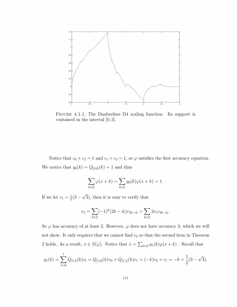
Figure 4.1.1. The Daubechies D4 scaling function. Its support iscontained in the interval [0, 3].
Notice that c0 + c2 = 1 and c1 + c3 = 1, so ϕ satisfies the first accuracy equation.
We notice that y0(k) = Q[0,0](k) = 1 and thus
∑k∈Z
ϕ(x+ k) =∑k∈Z
y0(k)ϕ(x+ k) = 1.
If we let v1 = 12(3−
√3), then it is easy to verify that
v1 =∑k∈Z
(−1)k(2k − di)c2k−di +∑k∈Z
2v1c2k−di .
So ϕ has accuracy of at least 2. However, ϕ does not have accuracy 3, which we will
not show. It only requires that we cannot find v2 so that the second item in Theorem
2 holds. As a result, x ∈ S(ϕ). Notice that x =∑
k∈Z y1(k)ϕ(x+ k) . Recall that
y1(k) =1∑t=0
Q[1,t](k)vt = Q[1,0](k)v0 +Q[1,1](k)v1 = (−k)v0 + v1 = −k +1
2(3−
√3).
111

Thus∑
k∈Z(−k + 12(3 −
√3))ϕ(x + k) = x. This is a rather remarkable fact that
an irregular function such as the D4 scaling function can perfectly reconstruct the
monomials 1 and x.
4.2. Accuracy
We will be adopting the notation used in [CHM]. We would like to stress that
the ideas in this chapter all come from[CHM]’s article on accuracy of the translates
of several refinable functions. In fact, if we have a refinable function f , we can look
at the accuracy of the translates of Lbfb∈B. This will be a special case of what is
covered in [CHM]. To determine the accuracy of the functions Lbfb∈B, we will have
to solve for a collection of row vectors vαα of dimension 1× |B|. Our contribution
is that in this special case, we only need to solve for a collection of scalars uαα,
therefore reducing the number of unknowns by a factor of |B|. This contribution is
enough that, in the next chapter, we can explicitly produce composite wavelets with
accuracy.
We will adopt the notation used in [CHM]. For any s ≥ 0, we define the column
vector of monomials Xs(x) = [xα]|α|=s. The total number of monomials of degree s
is ds =(s+n−1n−1
). We would like to find a generalization of the statement (ax)s = asxs
when a, x ∈ R. Let b be a n × n matrix with complex coefficients. We will define a
matrix bs so that Xs(bx) = bsXs(x). Now, notice (bx)α is a sum of monomials, where
each monomial is of degree s. So we can find bsα,β ∈ R such that∑|β|=s b
sα,βx
β = (bx)α.
Thus if we define the ds × ds matrix
(4.2.1) bs = [bsα,β]|α|=s,|β|=s
then
Xs(bx) = [(bx)α]|α|=s = [bsα,β]|α|=s,|β|=s[xβ]|β|=s = bsXs(x).
112
Next, we would like to generalize the statement (x−y)s =∑s
t=0Q[s,t](y)xt when x ∈ R.
For any multi-index α, (x− y)αis a polynomial of x of degree s = |α|. Let qα,β(y) be
such that (x−y)α =∑
0≤|β|≤s qα,β(y)xβ. Thus if we defineQ[s,t](y) = [qα,β(y)]|α|=s,|β|=t,
then
Xs(x− y) =[(x− y)α]|α|=s
=[∑
0≤|β|≤s
qα,β(y)xβ]|α|=s
=s∑t=0
[∑|β|=t
qα,β(y)xβ]|α|=s
=s∑t=0
[qα,β(y)]|α|=s,|β|=t[xβ]|β|=t
=s∑t=0
Q[s,t](y)Xt(x).
Explicitly, we may calculate qα,β(y). For any α, we have
(x− y)α =(x1 − y1)α1 · · · (xn − yn)αn
=n∏i=1
αi∑βi=0
(αiβi
)(−y)αi−βixβi
=
α1∑β1=0
· · ·αn∑βn=0
(α1
β1
)· · ·(αnβn
)(−y)α−βxβ.
If we define(αβ
)=(α1
β1
)· · ·(αnβn
)when β ≤ α and
(αβ
)= 0 if βi > αifor some i, then
(x− y)α =∑β≤α
(α
β
)(−y)α−βxβ.
Thus qα,β(y) =(αβ
)(−y)α−β.
113

Now, let γ ∈ I be an isometry on Rn. Then there exists an orthogonal matrix b
and y ∈ Rn such that γ = bty. We have
Xs(γx) = Xs(bx− by) = bsXs(x− y) = bs
s∑t=0
Q[s,t](y)Xt(x) =s∑t=0
bsQ[s,t](y)Xt(x).
For this reason, we will define
Q[s,t](bty) = bsQ[s,t](y).
Observe, if γ = ty,then Q[s,t](ty) = Q[s,t](y), so extending our definition of Q[s,t] agrees
with the original definition. According to this definition, we have
Xs(γx) =s∑t=0
Q[s,t](γ)(x)Xt(x).
This gives us to correct generalization of (x− y)s =∑s
t=0Q[s,t](y)xt when x ∈ R.
We are now going to state some useful results in [CHM]. This is Lemma 4.2 in
[CHM].
Lemma 56. Let a, b be n× n matrices. The following are true.
(1) If a is a scalar, then as = as.
(2) We have a0 = 1 and a1 = a.
(3) We have (ab)s = asbs. Thus if a is invertible then a−1s = (a−1)s.
(4) If a is expansive, then so is as.
The following is Lemma 4.3 in [CHM].
Lemma 57. Let b be an invertible matrix. If 0 ≤ t ≤ s and y ∈ Rn, then
Q[s,t](by) = bsQ[s,t](y)b−1t .
As a consequence, we have the following.
114

Lemma 58. Let c ∈ GLn(Rn). Then for any γ ∈ I, Q[s,t](cγc−1) = csQ[s,t](γ)c−1
t .
Proof. Let γ ∈ Γ , then for some b, x we have γ = btx. Thus cγc−1 = (cbc−1)tcx.
So
Q[s,t](cγc−1) = (cbc−1)sQ[s,t](cy)
= csbsc−1s Q[s,t](cy)
= csbsQ[s,t](y)c−1t
= csQ[s,t](γ)c−1t .
Proposition 59. We have
(1) Q[s,s](γ) = bs where γ = bty.
(2) Q[s,0](γ) = X[s](γ(0)).
(3) If 0 ≤ t ≤ s, then Q[s,t](γη) =∑s
u=tQ[s,u](γ)Q[u,t](η).
Proof. If |α| = |β| = s , then(αβ
)= 1 if α = β and
(αβ
)= 0 otherwise.
So for any y ∈ Rn we have qsα,β(y) = 1 if α = β and qsα,β(y) = 0 for α 6= β. Thus
Q[s,s](y) = I. Thus for any γ = bty we have Q[s,s](γ) = bsQ[s,s](y) = bs. For the second
assertion, we have qsα,0(y) = (−1)αyα = (−1)syα. Thus Q[s,0](y) = (−1)sXs(y). So
Q[s,0](bty) = bsQ[s,0](y) = (−1)sbsXs(y) = Xs(−by) = Xs(γ(0)). Next, let γ = bty and
η = ctz. Then
Q[s,t](γη) =Q[s,t](bctc−1y+z)
=(bc)sQ[s,t](c−1y + z)
=s∑u=t
(bc)sQ[s,u](c−1y)Q[u,t](z)
115

=s∑u=t
bsQ[s,u](y)cuQ[u,t](z)
=s∑u=t
Q[s,u](γ)Q[u,t](η).
For any s ≥ 0, let vα|α|≤s be a collection of scalars in C. For each 0 ≤ t ≤ s
we will sort scalars vα with |α| = t into the column vector vt = [vα]|α|=t. Given such
a collection of scalars vα|α|≤s , and any γ ∈ I, we define ys(γ) =∑s
t=0 Q[s,t](γ)vt.
Observe
ys(γη) =s∑t=0
Q[s,t](γη)vt
=s∑t=0
s∑u=t
Q[s,u](γ)Q[u,t](η)vt
=s∑
u=0
u∑t=0
Q[s,u](γ)Q[u,t](η)vt
=s∑
u=0
Q[s,u](γ)yt(η).
These ys appear quite naturally in a function with with accuracy, as shown in the
following theorem.
Theorem 60. Let f : Rn → C be an integrable function with independent shifts.
Assume f has accuracy p ≥ 1. Then there exists a collection of scalars vα|α|<p ,
with v0 6= 0, so that if we define vt = [vα]|α|=t and ys(γ) =∑s
t=0Q[s,t](γ)vt, then for
each 0 ≤ s < p we have
Xs(x) =∑γ∈Γ
ys(γ)f(γ−1x).
116

Proof. Let s ≥ 0 and αbe any multi-index with |α| = s. Then there exists
wα(γ) ∈ C so that
xα =∑γ∈Γ
wα(γ)f(γ−1x).
We group the wα(γ) together into a column vector ws(γ) = [wα(γ)]|α|=s. Thus
Xs(x) =∑
γ∈Γws(γ)f(γ−1x). Now,
Xs(ηx) =∑γ∈Γ
ws(γ)f(γ−1ηx) =∑γ∈Γ
ws(ηγ)f(γ−1x).
But we also have
Xs(ηx) =s∑t=0
Q[s,t](η)Xs(x) =∑γ∈Γ
s∑t=0
Q[s,t](η)wt(γ)f(γ−1x).
By using the independence of f(γ−1x) we have for all η, γ ∈ Γ that ws(ηγ) =∑st=0 Q[s,t](η)ws(γ). Define vt = wt(1). Setting γ = 1 we obtain
ws(η) =s∑t=0
Q[s,t](η)vt.
Thus if we define ys(γ) =∑s
t=0 Q[s,t](γ)vt, then Xs(x) =∑
γ∈Γ ys(γ)f(γ−1x). We also
have y0(γ) = Q[0,0](γ)v0 = v0 and so v0
∑γ∈Γ f(γ−1x) = 1 and thus v0 6= 0.
This remarkable fact demonstrates that ws(γ) only depend on the values of ws(1).
Notice this theorem holds regardless if f is refinable. So we will now consider the
case when f is refinable. Assume there exists a sequence of scalars cγγ∈Γ with all
but finitely many cγ = 0 so that
f(x) =∑γ∈Γ
cγf(γax).
Under this assumption we can prove the following.
117

Theorem 61. Let f : Rn → C be a refinable integrable function with independent
shifts. If f has accuracy p ≥ 1, then there exist scalars vα|α|<p , with v0 6= 0, so
that if we define vt = [vα]|α|=t for 0 ≤ t < p and ys(γ) =∑s
t=0Q[s,t](γ)vt we have
(1) Xs(x) =∑
γ∈Γ ys(γ)f(γ−1x) for all 0 ≤ s < p
(2) For all η ∈ Γ we have ys(η) =∑
γ∈Γ asys(γ)cη−1aγa−1.
Proof. We have,
Xs(a−1x) =
∑γ∈Γ
ys(γ)f(γ−1a−1x)
=∑γ,η∈Γ
ys(γ)cηf(ηaγ−1a−1x)
=∑η∈Γ
∑γ∈Γ
ys(γ)cη−1aγa−1f(η−1x)
which can also be written as
Xs(a−1x) = a−1
s Xs(x) =∑η∈Γ
a−1s ys(η)f(η−1x)
By independence of shifts, we have ys(η) =∑
γ∈Γ asys(γ)cη−1aγa−1 for all η ∈ Γ.
The following Theorem follows the proof of Theorem 4.6 in [CHM]. We include
a proof for completeness and to verify it still holds when we shift by elements in a
crystallographic group Γ. It is essentially identical to the proof given in [CHM].
Theorem 62. Let f ∈ L1(Rn) be a compactly supported integrable and refinable
function with a finitely supported refinement mask cγγ∈Γ. If there exists scalars
vα|α|≤s so that v0f(0) 6= 0 and for all 0 ≤ s < p and all η ∈ Γ we have ys(η) =∑γ∈Γ asys(γ)cη−1aγa−1, then f has accuracy p. Recall we have defined
ys(γ) =s∑t=0
Q[s,t](γ)vt
118

and vt = [vα]|α|=t . Furthermore,
CXs(x) =∑γ∈Γ
ys(γ)f(γ−1x)
where C = v0|E|−1f(0) and E is any fundamental domain for Γ.
Proof. Recall that there is a c ∈ GLn(R) so that L = cZn. Define A = c−1ac.
So A maps Zn to Zn and so it induces a homomorphism σ from Tn = Rn/Zn to itself
by σ(x + Zn) = Ax + Zn. Since A is expanding, then by Corollary 1.10.1 in [Walt],
σ is ergodic. Since the mapping x+Zn 7→ cx+L is a topological group isomorphism,
then the mapping τ : Rn/L → Rn/L given by τ(x+ L) = ax+ L is ergodic. We will
let T = c[−1/2, 1/2)n. T is a fundamental domain for L. So then τ is a mapping
from T onto T .
Now, define Hs(x) =∑
γ∈Γ ys(γ)f(γ−1x). The Hs(x) is well defined since all but
finitely many of the terms are nonzero. We have
Hs(ηx) =∑γ∈Γ
ys(γ)f(γ−1ηx)
=∑γ∈Γ
ys(ηγ)f(γ−1x)
=∑γ∈Γ
s∑t=0
Q[s,t](η)yt(γ)f(γ−1x) =s∑t=0
Q[s,t](η)Ht(x).
We also have,
Hs(a−1x) =
∑γ∈Γ
ys(γ)f(γ−1a−1x)
=∑γ∈Γ
∑η∈Γ
ys(γ)cηf(ηaγ−1a−1x)
=∑γ∈Γ
∑η∈Γ
ys(γ)cη−1aγa−1f(η−1x)
119

=a−1s
∑η∈Γ
ys(η)f(η−1x)
=a−1s Hs(x).
We will prove by induction on s that Hs(x) = CXs(x) for some scalar C 6= 0. First,
observe that H0(ηx) = Q[0,0](η)H0(x) = H0(x) and H0(a−1x) = a−10 H0(x) = H0(x).
Hence H0 is invariant under Γ and a . In fact, we simply have H0 is invariant under
L and a. This implies that H0(τ(x)) = H0(x) for all x ∈ T . Since τ is ergodic, then
H0(x) = C for almost all x ∈ Rn. We have
C = H0(x) =∑γ∈Γ
y0(γ)f(γ−1x) = v0∑γ∈Γ
f(γ−1x).
Let E denote any fundamental domain for Γ, which exists by Lemma 5, then inte-
grating both sides of the equation above yields
C|E| = v0
ˆE
∑γ∈Γ
f(γ−1x) dx
= v0
ˆRnf(x) dx
= v0f(0).
Thus C = v0|E|−1f(0). Therefore, f has accuracy at least 1.
Now, define Ws(x) = Hs(x) − CXs(x). Then Ws(ηx) = Hs(ηx) − CXs(ηx) =
Hs(x)− CXs(x). Also,
Ws(ηx) =Hs(ηx)− CXs(ηx)
=Hs(x)− CXs(x) +s−1∑t=0
Q[s,t](η)(Ht(x)− CXt(x))
=Ws(x).
120
We also have Ws(a−1x) = a−1
s Ws(x). Now, let M > 0 and define EM = x ∈ T :
||Ws(x)|| ≤ M. Let G0 = x ∈ T : Ws(x) 6= 0. Let SN(x) = n : 1 ≤ n ≤
N and ||Ws(anx)|| ≤ M. Notice that since Ws is L periodic, then ||Ws(a
nx)|| ≤ M
if and only if τn(x) ∈ EM . So we may write SN(x) = n : 1 ≤ n ≤ N and τn(x) ∈
EM. Since a is expansive, then so is as by Lemma 56. So thenWs(anx) = ansWs(x)→
∞ as n→∞ for any x ∈ G0. Hence for any x ∈ G0, we have
|SN(x)|N
→ 0
as N → ∞. However, by the remark following the Ergodic Theorem in [Walt], we
have for almost all x ∈ T ,|SN(x)|N
→ |EM |.
Assume G0 has positive measure. Then |EM | = 0 for all M > 0. However, |EM | > 0
for some M > 0, a contradiction. So we must conclude that |G0| = 0 and thus
Ws(x) = 0 for almost all x ∈ T . Therefore Ws(x) = 0 for all x ∈ Rn.
We can reformulate the second condition in the theorem above. First, we have
aΓa−1 is a subgroup of Γ. Let Γi| det a|i=1 denote the left cosets of Γ/aΓa−1. We then
have.
Theorem 63. The following are equivalent,
(1) For all 0 ≤ s < p, we have for all η ∈ Γ,
ys(η) =∑γ∈Γ
asys(γ)cη−1aγa−1
.
(2) For all 0 ≤ s < p, we have for each i = 1, . . . , | det a|,
vs =∑γ∈Γi
s∑t=0
Q[s,t](γ)atvtcγ
121

.
Proof. Assume we have the first item. Let γi be a coset representative of Γi.
We have
vs =ys(1)
=ys(γ−1i γi)
=s∑t=0
Q[s,t](γ−1i )yt(γi)
=s∑t=0
∑γ∈Γ
Q[s,t](γ−1i )atyt(γ)cγ−1
i aγa−1
=∑γ∈Γ
s∑t=0
t∑u=0
Q[s,t](γ−1i )atQ[t,u](γ)vucγ−1
i aγa−1
=∑γ∈Γ
s∑u=0
s∑t=u
Q[s,t](γ−1i )Q[t,u](aγa
−1)atvucγ−1
i aγa−1
=∑γ∈Γ
s∑u=0
Q[s,t](γ−1i aγa−1)atv
ucγ−1i aγa−1 .
Which is precisely vs =∑
γ∈Γi
∑st=0 Q[s,t](γ)atv
tcγ. Conversely, let γ ∈ Γ, then form
some i and η0 ∈ Γwe have γ−1 = γiaη0a−1 . Thus
ys(γ) =s∑t=0
Q[s,t](γ)vt
=s∑t=0
t∑u=0
∑η∈Γ
Q[s,t](γ)Q[t,u](γiaηa−1)auv
ucγiaηa−1
=∑η∈Γ
s∑u=0
s∑t=u
Q[s,t](γ)Q[t,u](γiaηa−1)auv
ucγiaηa−1
=∑η∈Γ
s∑u=0
Q[s,u](γγiaηa−1)auv
ucγiaηa−1
122

=∑η∈Γ
s∑u=0
Q[s,u](aη−10 ηa−1)auv
ucγiaηa−1
=∑η∈Γ
s∑u=0
asQ[s,u](η)vucγiaη0ηa−1
=∑η∈Γ
asys(η)cγ−1aηa−1.
4.3. Compactly Supported Composite Wavelets on R.
We are now ready to construct examples of compactly supported MRA wavelets.
We let B = 1,−1 be the identity and reflection of R. We let Γ = BZ and the
dilation a = 2. We let our fundamental domain F = [0, 1/2] and P = [−1/2, 1/2].
First, assume ϕ ∈ L2(R) is a compactly supported real valued scaling function for a
(2, BZ)-MRA. Then ϕ is refinable. Thus there exists cγγ∈Γ so that
ϕ(x) =∑γ∈Γ
cγϕ(γ(2x)),
with convergence in L2(R). We want a real valued ϕ, so we will assume cγ ∈ R for
all γ ∈ Γ. Recall from the equation 2.6.2 in Chapter 2, we have for all γ ∈ Γ we have
cγ = | det a|1/2〈ϕ,D1/2Lγ−1ϕ〉. Since we are assuming that ϕ has compact support,
then this equation implies that cγγ∈Γ has finite support. We let Λ = γ ∈ Γ : cγ 6=
0. Recall, the low-pass filter M0 for this function ϕ is given by
M0 =1
2
∑γ∈Λ
cγUγ−1 .
In this case, Θa = I. At the very least, we need M0 to satisfy the Smith-Barnwell
equation. Recall, this means, for all ξ ∈ P we have
M0(ξ)M0(ξ)∗ +M0(ξ + 1/2)M0(ξ + 1/2)∗ = I.
123

Notice we have replaced the phrase “almost everywhere” with “everywhere” because
M0 is now continuous. The Smith-Barnwell equation implies that M0 has a par-
ticular structure. We will now determine this structure. Recall for any d ∈ B we
haveU ξtk
(δd) = e2πiξd−1kδd. This implies
U ξtk
=
e2πiξk 0
0 e−2πiξk
.We also have
U ξ(−1)tk
= U ξ(−1)U
ξtk
=
0 1
1 0
e2πiξk 0
0 e−2πiξk
=
0 e−2πiξk
e2πiξk 0
.We will let a(ξ) = 1
2
∑k∈Z ctke
−2πiξk and b(ξ) = 12
∑k∈Z c(−1)tke
−2πiξk. Notice the
inverse of (−1)tk is equal to (−1)tk. Thus
M0(ξ) =1
2
∑k∈Z
ctkUξt−k
+1
2
∑k∈Z
c(−1)tkUξ(−1)tk
=
a(ξ) b(ξ)
b(−ξ) a(−ξ)
.Since we are assuming cγ are real, then a(ξ) = a(−ξ) and b(ξ) = b(−ξ). So
M0(ξ)M0(ξ)∗ =
|a(ξ)|2 + |b(ξ)|2 2a(ξ)b(ξ)
2a(−ξ)b(−ξ) |a(−ξ)|2 + |b(−ξ)|2
.Thus the Smith-Barnwell equation is equivalent to
(4.3.1) |a(ξ)|2 + |b(ξ)|2 + |a(ξ + 1/2)|2 + |b(ξ + 1/2)|2 = 1
and
(4.3.2) 2a(ξ)b(ξ) + 2a(ξ + 1/2)b(ξ + 1/2) = 0.
124

The equation 4.3.2 says that the vector (a(ξ), a(ξ + 1/2)) is orthogonal to the vec-
tor (b(ξ), b(ξ + 1/2)) in C2. Whenever the vector (a(ξ), a(ξ + 1/2)) is non-zero, it’s
orthogonal complement in C2 are multiples of the vector (a(ξ + 1/2),−a(ξ)). Since
(a(ξ), a(ξ + 1/2)) is non-zero almost everywhere, then there exists a trigonometric
polynomial λ(ξ) so that b(ξ) = λ(2ξ)e2πiξa(ξ + 1/2). Next, we plug this into the first
equation above to obtain,
(1 + |λ(2ξ)|2)(|a(ξ)|2 + |a(ξ + 1/2)|2) = 1.
Now, since the only units in the ring of Laurent polynomials are of the form ce2πiξk
where c ∈ C and k ∈ Z, then 1 + |λ(2ξ)|2 = K where K ∈ R. Thus |λ(2ξ)|2 = 1−K
is constant. This implies there exists λ0 ∈ Cand J ∈ Z so that λ(ξ) = λ0e2πiξ(2J+1).
Hence we can write,
b(ξ) = λ0e2πiξ(2J+1)a(ξ + 1/2).
In order for the coefficients of b to be real, we must have λ0 ∈ R. Therefore, we may
write
M0(ξ) =
a(ξ) λ0e2πiξ(2J+1)a(ξ + 1/2)
λ0e−2πiξ(2J+1)a(−ξ + 1/2) a(−ξ)
.Also, using the fact that b(ξ) = λ0e
2πiξ(2J+1)a(ξ + 1/2) and equation 4.3.1, we have
|a(ξ)|2 + |a(ξ + 1/2)|2 =1
1 + λ20
.
We summarize the discussion above in the next Proposition.
Proposition 64. Let M0 be in MΓ and assume the coefficients of M0 are real.
Assume all but finitely many of the cγ are non-zero. Then M0 satisfies the Smith-
Barnwell equation if and only if there exists a trigonometric polynomial a(ξ), J ∈ Z,
125

and λ0 ∈ R so that
M0(ξ) =
a(ξ) λ0e2πiξ(2J+1)a(ξ + 1/2)
λ0e−2πiξ(2J+1)a(−ξ + 1/2) a(−ξ)
,with |a(ξ)|2 + |a(ξ + 1/2)|2 = 1/(1 + λ2
0).
This form for M0 dramatically simplifies our problem of determining a suitable
low-pass filter. A very important feature of this representation of M0 is that we can
easily determine a high-pass filter.
Theorem 65. Let M0 be given as above. Define M1 as
(4.3.3) M1(ξ) = U ξt4J+2
−e−2πiξ(2J+1)a(ξ + 1/2) λ0a(ξ)
λ0a(−ξ) −e2πiξ(2J+1)a(−ξ + 1/2)
,then M1 satisfies
M1(ξ)M0(ξ)∗ +M1(ξ + 1/2)M0(ξ + 1/2)∗ = 0
and
M1(ξ)M1(ξ)∗ +M1(ξ + 1/2)M1(ξ + 1/2)∗ = I.
Proof. We can ignore the term U ξt4J+2
term because it is 12Z-periodic. So it
suffices to prove that the two equations hold if we simply define
M1(ξ) =
−e−2πiξ(2J+1)a(ξ + 1/2) λ0a(ξ)
λ0a(−ξ) −e2πiξ(2J+1)a(−ξ + 1/2)
.In fact, we will see later that the term U ξ
t4J+2ensures the scaling function and wavelet
share the same support. Now, we have
126

M1(ξ)M0(ξ)∗ =
c1(ξ) d1(ξ)
d1(−ξ) c1(−ξ)
,where
c1(ξ) = (1− λ20)e−2πiξ(2J+1)a(ξ)a(ξ + 1/2)
and
d1(ξ) = −λ0a(−ξ + 1/2)a(ξ + 1/2) + λ0a(−ξ)a(ξ).
Thus c1(ξ) + c1(ξ + 1/2) = 0 and d1(ξ) + d1(ξ + 1/2) = 0. Therefore,
M1(ξ)M0(ξ)∗ +M1(ξ + 1/2)M0(ξ + 1/2)∗ = 0.
We also have
M1(ξ)M1(ξ)∗ =
c2(ξ) d2(ξ)
d2(−ξ) c2(−ξ)
,where
c2(ξ) = λ20|a(ξ)|2 + |a(ξ + 1/2)|2
and
d2(ξ) = −λ0e−2πiξ(2J+1)
(a(ξ + 1/2)a(−ξ) + a(ξ)a(−ξ + 1/2
).
Thus c2(ξ) + c2(ξ + 1/2) = 1 and d2(ξ) + d2(ξ + 1/2) = 0. Hence,
M1(ξ)M1(ξ)∗ +M1(ξ + 1/2)M1(ξ + 1/2)∗ = I.
We are now going to place additional restrictions on a(ξ). If ϕ has a low-pass
filter M0, we will shift ϕ so that its support is contained in some interval of the form
127

[0, A]. Now, let k0 ∈ Z, then
U ξt2k0
M0(ξ)U ξt−k0
=
e2πiξk0a(ξ) e2πiξ2k0b(ξ)
e−2πiξ2k0b(−ξ) e−2πiξk0a(−ξ)
.If ϕ given by F(ϕ) = Utk0F(ϕ), then it is a scaling function for the exact same MRA
as ϕ with low-pass filter M0 = Ut2k0M0Ut−k0 . So we mary replace ϕ with ϕ and M0
with M0. For an appropriate choice of k0, we can assume that for some N ∈ N we can
write a(ξ) as a(ξ) = 12
∑Nk=0 ctke
−2πiξk so that ct0 6= 0 and ctN 6= 0. Now, we examine
the equation
|a(ξ/2)|2 + |a(ξ/2 + 1/2)|2 =1
1 + λ20
.
In terms of Fourier series, we have
|a(ξ/2)|2 =1
4
∑k,l∈Z
ctkctle−πiξ(k−l) =
1
4
∑k,l∈Z
ctkctk−le−πiξl.
So then,
|a(ξ/2)|2 + |a(ξ/2 + 1/2)|2 =1
4
∑k,l∈Z
ctkctk−l(e−πiξl + e−πiξl−πil)
=1
2
∑k,l∈Z
ctkctk−2le−2πiξl.
Therefore,
1
2
N∑k=0
ctkctk−2l=
1/(1 + λ2
0) for l = 0
0 for l 6= 0.
Suppose N were even. Then for some l we have 2l = N . Thus∑N
k=0 ctkctk−N = ctN ct0
and by the equation above we must have ctN ct0 = 0. However, this contradicts our
assumption that ct0 6= 0 and ctN 6= 0. Thus N must be odd. To summarize, we
will assume that for some odd N ∈ N that ctk = 0 for k < 0 and k > N and
128

that ct0 6= 0 and ctN 6= 0. We will now determine the coefficients c(−1)tk in terms of
ctk . Recall,
b(ξ) = λ0e2πiξ(2J+1)a(ξ + 1/2)
=1
2
∑k∈Z
(−1)kλ0ctke2πiξ(2J+1)e−2πiξk
=1
2
∑k∈Z
(−1)k+1λ0ct(k+2J+1)e−2πiξk.
Since we can also write b(ξ) = 12
∑k∈Z c(−1)tke
−2πiξk, then we can conclude
c(−1)tk = (−1)k+1λ0ct(k+2J+1).
Thus, we may restate Proposition 64.
Proposition 66. Let cγγ∈Γ be a real-valued and finitely supported. Assume
that for some odd N ∈ N that ctk = 0 for k < 0 and k > N and that ct0 6= 0 and
ctN 6= 0. DefineM0 = 12
∑γ∈Γ cγUγ−1. ThenM0 satisfies the Smith-Barnwell equation
if and only if for some λ0 ∈ R and J ∈ Z we have
c(−1)tk = (−1)k+1λ0ct(k+2J+1)
and
(4.3.4)1
2
N∑k=0
ctkctk−2l=
1/(1 + λ2
0) for l = 0
0 for l 6= 0.
In practice, we will use this Proposition instead of using the form given directly
on M0. We will now examine the coefficients of the high-pass filter. We write
129
M1 =1
2
∑γ∈Γ
dγUγ−1 .
So then a wavelet ψ can be written in terms of ϕ. We have
ψ(x) =∑γ∈Γ
dγϕ(γ(2x)).
We will now express the dγγ∈Γ in terms of cγγ∈Γ. We have
M1(ξ) =1
2
∑γ∈Γ
dγUξγ−1
=1
2
∑k∈Z
dtkUξt−k
+1
2
∑k∈Z
d(−1)tkUξ(−1)tk
.
We write m(ξ) = 12
∑k∈Z dtke
−2πiξk and n(ξ) = 12
∑k∈Z d(−1)tke
−2πiξk, then
M1(ξ) =
m(ξ) n(ξ)
n(−ξ) m(−ξ)
.Now, according to equation 4.3.3, M1 is given by
M1(ξ) = U ξt4J+2
−e−2πiξ(2J+1)a(ξ + 1/2) λ0a(ξ)
λ0a(−ξ) −e2πiξ(2J+1)a(−ξ + 1/2)
=
−e2πiξ(2J+1)a(ξ + 1/2) e2πiξ(4J+2)λ0a(ξ)
e−2πiξ(4J+2)λ0a(−ξ) −e−2πiξ(2J+1)a(−ξ + 1/2)
.So now we express m and n as a Fourier series. We have
m(ξ) = −e2πiξ(2J+1)a(ξ + 1/2)
=1
2
∑k∈Z
(−1)k+1ctke2πiξ(2J+1)e2πiξk
130
=1
2
∑k∈Z
(−1)k+1ct−2J−1−ke−2πiξk.
Next, for n we have
n(ξ) = λ0e2πiξ(4J+2)a(ξ)
=1
2
∑k∈Z
λ0ctke2πiξ(4J+2)e2πiξk
=1
2
∑k∈Z
λ0ct−4J−2−ke−2πiξk.
Therefore, we have determined dγ and they are given by
dtk = (−1)kct−2J−1−k and d(−1)tk = λ0ct−4J−2−k .
We can now rephrase Theorem 65 in terms of the coefficients dγγ∈Γ.
Theorem 67. Let M0 and cγγ∈Γ be as above. If we define M1 = 12
∑γ∈Γ dγUγ−1
where
dtk = (−1)kct−2J−1−k and d(−1)tk = λ0ct−4J−2−k ,
then M1 satisfies the equations in Theorem 65.
Although we have shown in the previous chapter that there always exists a high-
pass filter, it’s coefficients were not necessarily trigonometric polynomials. The im-
portance of the Theorem above and Theorem 65 is that if ϕ is a compactly supported
scaling function, then so is it’s associated wavelet ψ with F(ψ)(ξa) = M1(ξ)F(ϕ)(ξ).
In general, it is a very difficult algebraic problem to determine an appropriate M1 so
that dγγ∈Γ are finitely supported. Our next step will be to determine the J above.
We will choose J to minimize the support of ϕ.
131

Proposition 68. Let E be the compact set that satisfies
E =1
2
⋃γ∈Λ
γ−1E
where Λ = t0, t1, . . . , tM ∪ (−1)tI , . . . , (−1)tI+M. Then |E| is minimized with
I = Mand in this case E = [0,M ].
Proof. Observe that
1
2
M⋃k=0
([0,M ] + k) = [0,M ].
Thus [0,M ] ⊂ 12
⋃Mk=0 γ
−1[0,M ]. Thus [0,M ] ⊂ E. So then |E| is at least M . When
I = M , we have1
2
I+M⋃k=I
(−1)[0,M ] + k = [0,M ].
So when I = M , then E = [0,M ], which minimizes |E|.
We will now apply this proposition. Now, if ctk 6= 0, then 0 ≤ k ≤ N . Since
c(−1)tk = (−1)k+1λ0ct(k+2J+1), then if c(−1)tk 6= 0 , then−2J−1 ≤ k ≤ N−2J−1. Recall
Λ = γ ∈ Γ : cγ 6= 0. We let Λ′ = t0, t1, . . . , tN ∪ (−1)t−2J−1, . . . , (−1)tN−2J−1.
So Λ ⊂ Λ′. LetK ′ be the attractor of the iterative function systemK ′ = 12
⋃γ∈Λ′ γ
−1K ′.
We will minimize K ′ according to Proposition 68. By this proposition, K ′ is mini-
mized if we choose 2J + 1 = −N . For this choose K ′ = [0, N ]. Recall from Theorem
47 that the support of a scaling function ϕ with coefficients cγγ∈Γ is contained in the
attractor K of the iterative function system K = 12
⋃γ∈Λ γ
−1K. Since Λ ⊂ Λ′, then
K ⊂ K ′ = [0, N ]. So when 2J + 1 = −N , ϕ has support contained in [0, N ]. In gen-
eral, the support of ϕ can be very difficult to determine. This is why we concentrated
on simply minimizing K ′.
4.3.1. Our setup. We have covered quite a bit of technical material. So we
will review our approach to finding these compactly support composite wavelets. Let
132

N ∈ N be odd and λ0 ∈ R. Assume there exists scalars ctk ∈ R for 0 ≤ k ≤ N and
c(−1)tk ∈ R for N ≤ k ≤ 2N so that
(4.3.5) c(−1)tk = (−1)k+1λ0ct(k−N)
and
(4.3.6)1
2
N∑k=0
ctkctk−2l=
1/(1 + λ2
0) for l = 0
0 for l 6= 0.
Define cγ = 0 if γ /∈ Λ = t0, t1, . . . , tN∪(−1)tN , . . . , (−1)t2N. IfM0 = 12
∑γ∈Λ cγUγ−1 ,
then Proposition 64M0 will satisfy the Smith-Barnwell equation. We define v =
(1/√
2, 1/√
2)t. By Theorem 47, there exists a compactly support function ϕ ∈ L2(R)
with support in [0, N ] defined as
F(ϕ)(ξ) = limj→∞
M0(ξa−1)M0(ξa−2) · · ·M0(ξa−j)v.
Furthermore, ϕ satisfies F(ϕ)(0) = v and F(ϕ)(ξa) = M0(ξ)F(ϕ)(ξ) and ϕ(x) =∑γ∈Γ cγϕ(γ(2x)). Thus ϕ will satisfy the last two conditions of Theorem 29. It
remains to show the orthonormality of Lγϕγ∈Γ. If this collection is orthonormal,
then ϕ will be a scaling function for a MRA. We will use Theorem 51.
To construct the wavelet ψ, we define dtk = (−1)kcN−k for 0 ≤ k ≤ N and
d(−1)tk = λ0ct2N−k for N ≤ k ≤ 2N . Define dγ = 0 for all other γ ∈ Γ. By Theorem
67,M1 = 12
∑γ∈Λ dγUγ−1 will be a high-pass filter associated withM0. If ϕ is a scaling
function for a MRA, then
ψ(x) =∑γ∈Λ
dγϕ(γ(2x))
will be a (2,Γ)-MRA wavelet. Suppose x /∈ [0, N ], then x /∈ 12
⋃γ∈Λ γ
−1[0, N ]. Thus
γ(2x) /∈ [0, N ] for all γ ∈ Λ. Since suppϕ ⊂ [0, N ], then ϕ(γ(2x)) = 0 for all γ ∈ Λ.
By the relationship between ψ and ϕ this implies ψ(x) = 0. Hence suppψ ⊂ [0, N ].
133

4.3.2. Orthogonality of Lγϕγ∈Γ. The remaining condition to verify is the
orthogonality of Lγϕγ∈Γ. Once we have the coefficients cγγ∈Γ, we will verify the
two conditions of Theorem 51. First we examine the rank-condition onM0(0). Recall
we have
M0(0) =
a(0) λ0a(1/2)
λ0a(1/2) a(0)
.Notice we have F(ϕ)(0) = M0(0)F(ϕ)(0) where F(ϕ)(0) = (1/
√2, 1/√
2)t. This
implies that a(0) + λ0a(1/2) = 1. Recall, the Smith-Barnwell equation implies
M0(0)M0(0)∗ +M0(1/2)M0(1/2)∗ = I.
Since F(ϕ)(0) = M0(0)F(ϕ)(0), then by the symmetry ofM0(0) we also have F(ϕ)(0) =
M0(0)∗F(ϕ)(0). Thus
F(ϕ)(0) = M0(0)M0(0)∗F(ϕ)(0) +M0(1/2)M0(1/2)∗F(ϕ)(0)
= F(ϕ)(0) +M0(1/2)M0(1/2)∗F(ϕ)(0).
Subtracting F(ϕ)(0) from both sides yields M0(1/2)M0(1/2)∗F(ϕ)(0) = 0 and thus
M0(1/2)∗F(ϕ)(0) = 0. Since
M0(1/2)∗ =
a(1/2) −λ0a(0)
−λ0a(0) a(1/2)
,then a(1/2)− λ0a(0) = 0. Combining this with a(0) + λ0a(1/2) = 1, then we obtain
a(0) = 1/(1 + λ20) and a(1/2) = λ0/(1 + λ2
0). Therefore,
M0(0) =1
1 + λ20
1 λ20
λ20 1
.
134

Notice w1 = (1, 1)t and w2 = (1,−1)t are eigenvectors of M0(0) with eigenvalues 1
and (1 − λ20)/(1 + λ2
0), respectively. The rank-condition on M0(0) is that the only
eigenvalues of modulus 1 of M0(0) is 1 and this eigenspace has dimension one. So
assume (1 − λ20)/(1 + λ2
0) has absolute value 1. Then (1 − λ20)/(1 + λ2
0) = 1 or
(1 − λ20)/(1 + λ2
0) = −1. The second case cannot hold for any λ0. The first case
implies λ0 = 0. To summarize, M0(0) satisfies the rank-condition of Theorem 51 if
and only if λ0 6= 0.
Next, we examine equation 3.5.2. Recall, the equation defines a matrix M by
(4.3.7) M =
[1
| det a|∑ω∈Γ
cωcη−1ωaγa−1
]γ,η∈Λ∗
.
Here Λ∗ is the set of γ ∈ Γ so that Lγϕ and ϕ have disjoint support. In this case, it
is easy to verify that
Λ∗ = t−N+1, t−N+2, . . . , tN−1 ∪ (−1)t1, (−1)t2, . . . , (−1)t2N−1.
By Theorem 51, Lγϕγ∈Γ forms an orthonormal basis if and only if λ0 6= 0 and the
eigenvalue 1 of M has geometric multiplicity 1. We will not explicitly calculate M
or its eigenvalues. M can get very large and we will calculate its eigenvalues using a
computer.
4.3.3. Accuracy equations. We now examine the accuracy equations. Recall
from equation 4.2.1, for any c ∈ R we have cs = cs. Recall for any y ∈ R, we have
Q[s,t](bty) = bsQ[s,t](y) = bs(s
t
)(−y)s−t.
We will solve for v0, . . . , vp−1 so that for all 0 ≤ s < p and i = 1, 2,
vs =∑γ∈Γi
s∑t=0
Q[s,t](γ)atvtcγ.
135

We may assume v0 = 1. Observe Γ1 = B(2Z) and Γ2 = B(2Z + 1). Thus we write
for 0 ≤ s < p.
vs =∑γ∈Γ1
s∑t=0
Q[s,t](γ)atvtcγ
=∑k∈2Z
s∑t=0
Q[s,t](tk)2tvtctk +
∑k∈2Z
s∑t=0
Q[s,t]((−1)tk)2tvtc(−1)tk
=
(N−1)/2∑k=0
s∑t=0
Q[s,t](t2k)2tvtct2k +
N∑k=(N+1)/2
s∑t=0
Q[s,t]((−1)t2k)2tv2c(−1)t2k .(4.3.8)
We also have
vs =∑γ∈Γ2
s∑t=0
Q[s,t](γ)atvtcγ
=∑
k∈2Z+1
s∑t=0
Q[s,t](tk)2tvtctk +
∑k∈2Z+1
s∑t=0
Q[s,t]((−1)tk)2tvtc(−1)tk
=
(N−1)/2∑k=0
s∑t=0
Q[s,t](t2k+1)2tvtct2k +
(2N−1)/2∑k=(N−1)/2
s∑t=0
Q[s,t]((−1)t2k+1)2tv2c(−1)t2k+1.
(4.3.9)
These are the accuracy equations.
4.3.4. Examples. The simplest example of a compactly supported (2,Γ)-MRA
wavelet is the Haar wavelet. We define the scaling function ϕ =√
2χ[0,1/2) and it’s
associated wavelet ψ =√
2χ[0,1/4) −√
2χ[1/4,1/2). In this case, ϕ has accuracy 1. We
now produce more interesting examples. We fix an odd positive integer N ∈ N and
let p = (N + 3)/2. We then solve for cγγ∈Γ,vs0≤s<p, and λ0 from the equations
4.3.5,4.3.6,4.3.8, and4.3.9. When N = 1, we obtain a solution
ct0 =1
4(3−
√3) ct1 =
1
4(3 +
√3)
136

and
c(−1)t1 =1
4(1−
√3) c(−1)t2 =
1
4(1 +
√3).
The solution to the refinement equation ϕ(x) =∑
γ∈Γ cγϕ(γ(2x)) is a scaling function
for a (2,Γ)-MRA. This example was first discovered by Blanchard and Krishtal in
[BK]. It has accuracy 2.
Figure 4.3.1. The Blanchard-Krishtal wavelet. It is the first exampleof a compactly supported composite wavelet beyond the Haar wavelet.It has accuracy 2 and is supported in the interval [0, 1]. The figure onthe left is the scaling function and the figure on the right is the wavelet.
Explicitly, we have
ϕ(x) =
1√2
(2√
3x+ 1−√
3)
for x ∈ [0, 1]
0 for x /∈ [0, 1]
.
From this expression, it is easy to verify that Lγϕγ∈Γ is an orthonormal system. In
general, we will not have a simple expression for ϕ.
The examples to follow are new. We first solve the equations 4.3.5,4.3.6,4.3.8,
and4.3.9 using Mathematica. In all cases, λ0 6= 0 and so M0(0) satisfies the rank-
condition. Next, we produce the matrix M as in 4.3.7 and verify the eigenvalue 1 has
geometric multiplicity 1. For N = 3 and p = 3 we obtain the following coefficients:
137

ct0180
(15− 10
√6− 6
√10 + 5
√15)
ct1980
(5 +√
15)
ct2980
(5−√
15)
ct3180
(15 + 10
√6− 6
√10− 5
√15)
c(−1)t3180
(5 +√
15)
c(−1)t4−180
(15 + 10
√6 + 6
√10 + 5
√15)
c(−1)t5180
(15− 10
√6 + 6
√10− 5
√15)
c(−1)t6180
(5−√
15)
Table 1. Coefficients of the P -3 scaling function.
We must show that Lγϕγ∈Γ is an orthonormal system. The matrix M is the
following 10× 10 matrix:
0.0000 −0.0008 0.0000 0.0008 0.0000 0.0141 −0.0008 0.0000 0.0008 0.0141
0.5128 0.0082 0.0000 −0.0079 0.4872 0.4715 −0.1153 0.0281 0.1153 0.4715
0.0000 0.0004 1.0000 0.0004 0.0000 0.0281 0.2323 0.9431 −0.2323 0.0281
0.4872 −0.0079 0.0000 0.0082 0.5128 0.4715 −0.1153 0.0281 0.1153 0.4715
0.0000 0.0008 0.0000 −0.0008 0.0000 0.0141 −0.0008 0.0000 0.0008 0.0141
0.0000 −0.0063 0.0000 −0.0063 0.0000 −0.1136 0.0065 0.0000 0.0062 0.1079
0.0000 0.4933 0.0000 0.4933 0.0000 0.1249 0.4899 −0.0057 0.4661 −0.1187
0.0000 0.5059 0.0000 0.5059 0.0000 0.1097 0.4820 0.0062 0.5051 −0.1153
0.0000 0.0063 0.0000 0.0063 0.0000 −0.1187 0.0214 0.0001 0.0226 0.1249
0.0000 0.0001 0.0000 0.0001 0.0000 −0.0017 0.0001 0.0000 0.0001 0.0018
The eigenvalues, listed according to multiplicity, of this matrix are
1.000 0.2500 0.1357 −0.0576 0.0625
0.0007 0.0032 0.0032 0.0128 0.0128.
Since 1 occurs exactly once, then the conditions of Theorem 51 are satisfied and so
Lγϕγ∈Γ is an orthonormal system. Therefore, the solution, correctly normalized,
of the refinement equation ϕ(x) =∑
γ∈Γ cγϕ(γ(2x)) is a scaling function for a
(2,Γ)-MRA. This example has accuracy 3.
138

Figure 4.3.2. The P -3 wavelet. It is a compactly supported compositewavelet with accuracy 3. Both the scaling function and wavelet aresupported in the interval [0, 3]. This is the first example of a compositewavelet with accuracy higher than the Blanchard-Krishtal wavelet.
The rest of our examples follow a similar approach. We will not show the matrix M
nor it’s eigenvalues, but they all satisfy the conditions of Theorem 51as verified
using MatLab. We obtain more solutions for N = 5, 7,and9.
ct0 0.054594774872714365
ct1 −0.1860085771113526
ct2 0.9217210640146265
ct3 0.1499550068940092
ct4 −0.023224034245360188
ct5 −0.006816411054004981
λ0 1.0941967774637191
Table 2. Coefficients of the P -4 scaling function. The coefficientsc(−1)tk are determined by the formula c(−1)tk = (−1)k+1λ0ctk−N withN = 5. Here p = 4.
139
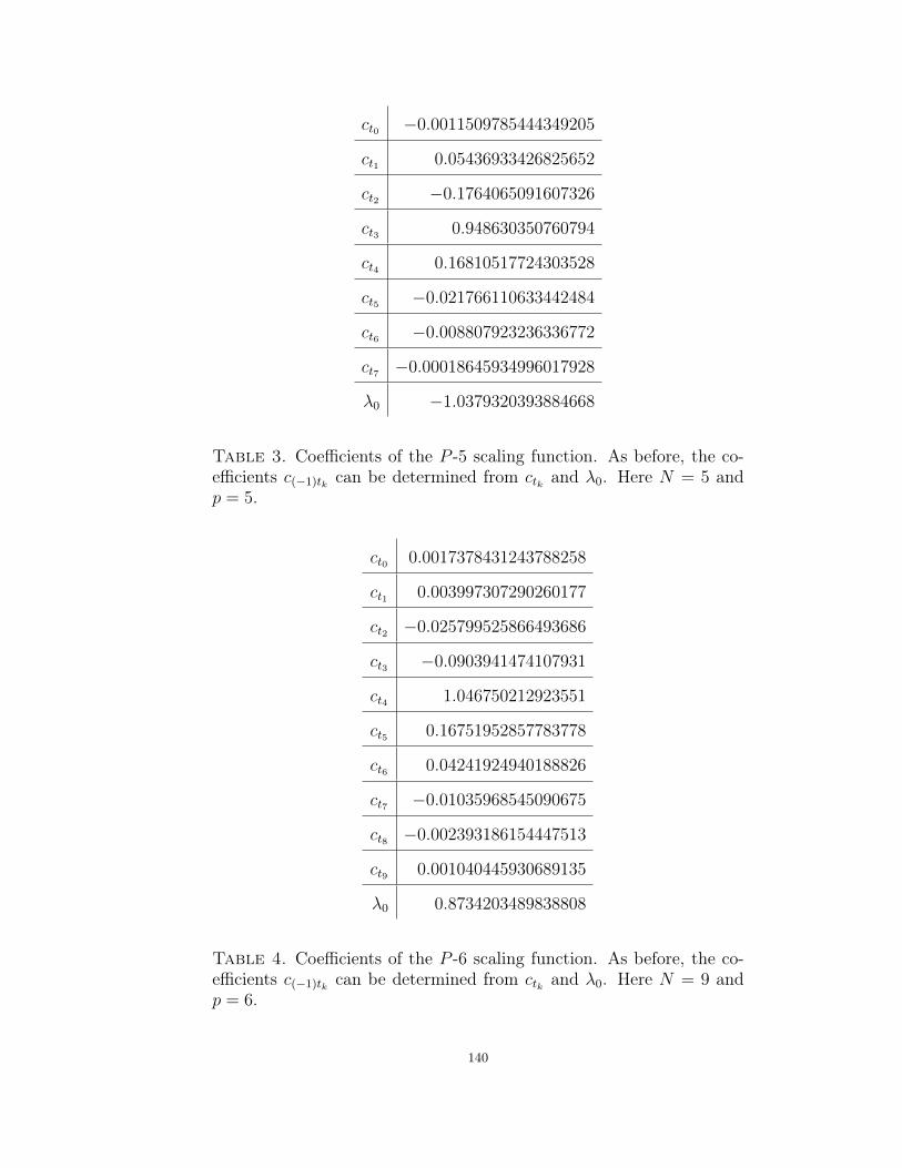
ct0 −0.0011509785444349205
ct1 0.05436933426825652
ct2 −0.1764065091607326
ct3 0.948630350760794
ct4 0.16810517724303528
ct5 −0.021766110633442484
ct6 −0.008807923236336772
ct7 −0.00018645934996017928
λ0 −1.0379320393884668
Table 3. Coefficients of the P -5 scaling function. As before, the co-efficients c(−1)tk can be determined from ctk and λ0. Here N = 5 andp = 5.
ct0 0.0017378431243788258
ct1 0.003997307290260177
ct2 −0.025799525866493686
ct3 −0.0903941474107931
ct4 1.046750212923551
ct5 0.16751952857783778
ct6 0.04241924940188826
ct7 −0.01035968545090675
ct8 −0.002393186154447513
ct9 0.001040445930689135
λ0 0.8734203489838808
Table 4. Coefficients of the P -6 scaling function. As before, the co-efficients c(−1)tk can be determined from ctk and λ0. Here N = 9 andp = 6.
140

We also have graphs of the scaling functions and wavelets.
Figure 4.3.3. The P -4 wavelet. It has accuracy 4 and is supportedin the interval [0, 5].
The graph above is the “p4” scaling function. It has accuracy 4.
Figure 4.3.4. The P -5 wavelet. It has accuracy 5 and is supportedin the interval [0, 7].
The graph above is the graph of a composite scaling function with accuracy 6.
141

Figure 4.3.5. The P -6 wavelet. It has accuracy 6 and is supportedin the interval [0, 9].
4.4. The Cascade Algorithm
Here we discuss how to produce the graphs in the previous section. Given a low-
pass filter, we can construct the Fourier transform of the scaling function through the
following limit,
F(ϕ)(ξ) = limk→∞
M0(2−1ξ) · · ·M0(2−kξ)F(ϕ)(0).
While this determines F(ϕ), it is quite an unwieldy form to explicitly determine the
values of ϕ. In most cases, ϕ will have no simple expression. In this section, we
produce an algorithm for explicitly determining the values of ϕ. On certain dyadic
sets, we may calculate the values of ϕ. Recall, the refinement equation is given by
ϕ(x) =∑γ∈Γ
cγϕ(γax).
Now, let k ∈ L. We have
ϕ(k) =∑γ∈Γ
cγϕ(γak)
=∑b∈B
∑l∈L
cbtlϕ(bak − bl)
142

=∑b∈B
∑l∈L
cbtak−b−1lϕ(l).
Let L0 = k ∈ L : ϕ(k) 6= 0. Thus, we define the matrix L = [∑
b∈B cbtak−b−1l]k,l∈L0 ,
then the column vector [ϕ(k)]k∈L0 is an eigenvector of L with eigenvalue one. So
assume we know cγγ∈Γ but not the values of ϕ. We first determine L0 and then
we find the eigenvectors of M with eigenvalue one. For example, the Proposition 68
tells a set which contains the support of ϕ and hence L0. Assuming the eigenspace
of eigenvalue one has dimension one for M then we know, up to multiplication by a
scalar, the vector v = [ϕ(k)]k∈L0 . Now, in our present setting, we have B = 1,−1,
L = Z, and a = 2. By Theorem 29, we must have ||F(ϕ)(0)|| = 1. This implies
ϕ(0) = 1/√
2. Also E = [0, 1/2) is a fundamental domain for Γ. By Theorem 62, we
have
2∑k∈Z
ϕ(k) =∑γ∈Γ
ϕ(γ(0)) = ϕ(0)|E|−1 =√
2.
Thus ∑k∈Z
ϕ(k) =1√2.
So if w is an eigenvector of L of eigenvalue 1 and the sum of its entries are equal to
1/√
2, then w = v = [ϕ(k)]k∈L0 . This approach allows us to determine the exact value
of ϕ on the lattice L. Now that we know the values of ϕ on L, we use the equation
ϕ(a−1x) =∑γ∈Γ
cγϕ(γx)
to explicitly determine the values of ϕ on a−1L. We apply this iteratively to determine
the values of ϕ on a−nL for any n ∈ N. As n gets larger, we know the values of ϕ
on a finer and finer lattice. This allows us to approximate the values of ϕ and will
give us its exact value on dyadic lattice points. This procedure was used to create
the graphs of composite scaling functions.
143

4.5. Conclusions
The examples of composite wavelets in this chapter are the analogue of Daubechies
wavelets. Our examples include composite wavelets with accuracy up to 6. To find
the coefficients for these wavelets we had to numerically solve the accuracy equations
and the Smith-Barnwell equations. After accuracy 6 this becomes a computationally
demanding problem. Simplifying these equations would allow us to produce more
examples of composite wavelets. In particular, it would be worthwhile rewriting
the equations in a form similar to the Strang-Fix conditions. For example, we did
incidentally simplify the accuracy equations for accuracy 1: a(0) = 1/(1 + λ20) and
a(1/2) = λ0/(1 + λ20). This is equivalent to
∑k∈Z
ck =1
1 + λ20
and∑k∈Z
(−1)kck =λ0
1 + λ20
.
In fact, we conjecture that we can find rational functions f s0 and f s1 for 0 ≤ s so that
accuracy p is equivalent to
∑k∈Z
ksck = f s0 (λ0) and∑k∈Z
(−1)kksck = f s1 (λ0) for0 ≤ s < p.
This form would eliminate the need to solve for vs0≤s<p in the accuracy equations.
Additionally, in this setting, it is reasonable to conjecture that ϕ has accuracy p if
and only if the first p moments of ψ are zero.
Next we would like to examine the smoothness of these functions. By making use
of the joint-spectral radius, [CH] provided a method to determine the smoothness of
refinable functions. Generalizing this to the composite case would be a logical step
towards determining the smoothness of our composite wavelets.
Finding examples in higher dimensions is difficult. We have shown how to produce
composite wavelets for any Γ in any dimension as long as | det a| = 2. However, these
examples are not compactly supported. We have provided a foundation for producing
144

compactly supported composite wavelets with accuracy in Chapters 3 and 4. Our
success in one dimension is a result of determining the exact form of the low-pass
filter M0. However, if we let B be the symmetries of the square in two dimensions,
Γ = BZ2, and a be the quincunx matrix, then M0 is a 8× 8 matrix. In this case it is
much more difficult to determine the form ofM0. It will involve a fair amount of work
to extend our results to higher dimension. In general, there may not be any simple
way to express the exact form of M0. It would be worthwhile to examine specific
forms of M0 and to produce examples of these compactly supported wavelets.
We have presented nice composite wavelets on R. However, there were many
other solutions whose graphs appeared fractal and not differentiable anywhere. Of
the compactly supported composite wavelets with accuracy, the nice examples were
the minority. This poses a serious problem in higher dimensions. Given the countless
possibilities for M0, we would have to sort through a large collection of wavelets
before finding the ones which have any degree of smoothness. Whether or not any
exist remains an open problem.
145

Bibliography
[CHM] C. Cabrelli, C. Heil, and U. Molter, “Accuracy of lattice translates of several multidi-
mensional refinable functions”, J. Approx. Theory, 95 (1998), 5-52.
[CHM2] U. Molter C. Cabrelli, C. Heil, Multiwavelets in Rn with an arbitray dilation matrix, in:
Wavelets and Signal Processing, L. Debnath,ed., Birkh¨auser , Boston (2003), 23–39.
[TLW] I. Daubechies, Ten lectures on wavelets, Society for Industrial and Applied Mathematics,
Philadelphia, 1992.
[HW] E. Hern´andez and G. Weiss, A first course on wavelets, Studies in Advanced Mathe-
matics. CRC Press, Boca Raton, FL, 1996.
[SB] K. Steffen J. Blanchard, Crystallographic haar-type composite dilation wavelets,
Wavelets and Multiscale Analysis (Jonathan Cohen and Amed I. Zayed, eds.), Applied
and Numerical Harmonic Analysis, Birkh¨auser Boston, 2011, pp. 83–108.
[BK] J. Blanchard and I. Krishtal, Matricial Filters for Crystallographic Composite Dilation
Wavelets, Mathematics of Computation, 81, 905-922, 2012.
[Law] Lawton, W., Necessary and sufficient conditions for constructing orthonormal wavelet
bases, J. Math. Phys. 32 (1991), 57-61.
[Walt] P. Walters, “An Introduction to Ergodic Theory,” Springer-Verlag, New York, 1982.
[CH] D. Colella and C. Heil, Dilation equations and the smoothness of compactly supported
wavelets, in: "Wavelets: Mathematics and Applications," J. J. Benedetto and M. W.
Frazier, eds., CRC Press, Boca Raton, FL (1994), 163-201.
[GLLWW] K. Guo, D. Labate, W. Lim, G. Weiss, and E. N. Wilson. The theory of wavelets
with composite dilations. In Harmonic analysis and applications, Appl. Numer.
Harmon. Anal., pages 231–250. Birkh¨auser Boston, Boston, MA, 2006.
[GLLWW2] K. Guo, D. Labate, W. Lim, G. Weiss, and E. N. Wilson. Wavelets with composite
dilations and their MRA properties.Appl. Comput. Harmon. Anal., 20(2):202–236,
2006.
146

[Hou] R. Houska. The nonexistence of shearlet-like scaling multifunctions that satisfy certain
min- imally desirable properties and characterizations of the reproducing properties of
the integer lattice translations of a countable collection of square integrable functions.
Ph.D. dissertation, 2009. Washington University in St. Louis.
[KRWW] I. Krishtal, B. Robinson, G. Weiss, and E. N. Wilson. Some simple Haar-type wavelets
in higher dimensions. J. Geom. Anal., 17(1):87–96, 2007.
[GM] K. Gröchenig and W. R. Madych, Multiresolution analysis, Haar bases, and self-similar
tilings of Rn, IEEE Trans. Inform. Theory 38 (1992), 556-568.
[Bow] M. Bownik, The structure of shift-invariant subspaces of L2(Rn), Journal of Func-
tional Analysis 177 (2000), no. 2, 282 – 309.
[BRS] M. Bownik, Z. Rzeszotnik, and D. Speegle, A characterization of dimension functions
of wavelets, Appl. Comput. Harmon. Anal. 10 (2001), 71-92.
[BW] M. A. Berger and Y. Wang, Multidimensional two-scale dilation equations, Wavelets:
A Tutorial in Theory and Applications, Wavelet Anal. Appl. 2, C. K. Chui, ed.,
Academic Press, New York, (1992), pp. 295–323.
[HSWW] E. Hernandez, H. Sikic, G. Weiss, and E. Wilson, On the properties of the integer
translates of a square integrable function. , Contemporary Mathematics, Vol. 505,
(2010) 233-249.
[HSWW2] E. Hernandez, H. Sikic, G. Weiss, and E. Wilson, Cyclic subspaces for unitary represen-
tations of LCA groups: generalized Zak transforms, Colloq. Math. 118 no. 1, (2010)
313-332.
[Tay] K. Taylor: C*-Algebras of Crystal Groups. Operator Theory: Advances and Ap-
plications, 41 511-518(1989).
[Rud] W. Rudin, Fourier analysis on groups, Interscience, New York 1962.
147


