

DI
SC
US
SI
ON
P
AP
ER
S
ER
IE
S
Forschungsinstitut zur Zukunft der ArbeitInstitute for the Study of Labor
Compulsory Schooling Laws and Formation of Beliefs:Education, Religion and Superstition
IZA DP No. 8698
December 2014
Naci MocanLuiza Pogorelova
Compulsory Schooling Laws and
Formation of Beliefs: Education, Religion and Superstition
Naci Mocan Louisiana State University,
NBER and IZA
Luiza Pogorelova Louisiana State University
Discussion Paper No. 8698 December 2014
IZA
P.O. Box 7240 53072 Bonn
Germany
Phone: +49-228-3894-0 Fax: +49-228-3894-180
E-mail: [email protected]
Any opinions expressed here are those of the author(s) and not those of IZA. Research published in this series may include views on policy, but the institute itself takes no institutional policy positions. The IZA research network is committed to the IZA Guiding Principles of Research Integrity. The Institute for the Study of Labor (IZA) in Bonn is a local and virtual international research center and a place of communication between science, politics and business. IZA is an independent nonprofit organization supported by Deutsche Post Foundation. The center is associated with the University of Bonn and offers a stimulating research environment through its international network, workshops and conferences, data service, project support, research visits and doctoral program. IZA engages in (i) original and internationally competitive research in all fields of labor economics, (ii) development of policy concepts, and (iii) dissemination of research results and concepts to the interested public. IZA Discussion Papers often represent preliminary work and are circulated to encourage discussion. Citation of such a paper should account for its provisional character. A revised version may be available directly from the author.

IZA Discussion Paper No. 8698 December 2014
ABSTRACT
Compulsory Schooling Laws and Formation of Beliefs: Education, Religion and Superstition*
We exploit information on compulsory schooling reforms in 11 European countries, implemented mostly in the 1960s and 70s, to identify the impact of education on religious adherence and religious practices. Using micro data from the European Social Survey, conducted in various years between 2002 and 2013, we find consistently large negative effects of schooling on self-reported religiosity, social religious acts (attending religious services), as well as solitary religious acts (the frequency of praying). We also use data from European Values Survey to apply the same empirical design to analyze the impact of schooling on superstitious beliefs. We find that more education, due to increased mandatory years of schooling, reduces individuals’ propensity to believe in the power of lucky charms and the tendency to take into account horoscopes in daily life. JEL Classification: I21, Z1 Keywords: religion, education, superstition, Europe, beliefs, praying Corresponding author: Naci Mocan Louisiana State University Department of Economics 3039 Business Education Complex Baton Rouge, LA 70803 USA E-mail: [email protected]
* We thank participants of the ASREC Conference in Durham England, and Daniel Chen, Jörg Spenkuch and David Voas for helpful comments.

1
Compulsory Schooling Laws and Formation of Beliefs:
Education, Religion and Superstition
“The state … derives no inconsiderable advantage from [the instruction
of uneducated citizens]. The more they are instructed the less liable they
are to the delusions of enthusiasm and superstition, which, among ignorant
nations, frequently occasion the most dreadful disorders.”
Adam Smith, The Wealth of Nations; V.1.189
I. Introduction
Education provides substantial private benefits to individuals. For example, education
increases productivity in the labor market, and raises earnings (Card 2001, Oreopoulos 2006,
Mocan 2014). More educated people are healthier because they are more efficient producers of
health (Chou, Liu, Grossman 2010, Grossman 2006). Also, they acquire new information better
and respond to it faster in comparison to those who are less educated (Lange 2011, Price and
Simon 2009). In addition, education provides social benefits in a variety of forms. Because
marketable skills and employment prospects are higher if workers are more educated, education
helps reduce negative externalities imposed on society through such vehicles as lower criminal
activity and reduced reliance on government transfers.
If education improves cognition and the ability for critical thinking, more educated
people should be less likely to believe in supernatural forces, suggesting that education should
reduce religiosity. In fact, a long line of philosophers and social scientists, ranging from
Durkheim to Weber, have argued that increased levels of education would diminish the need for
religious adherence. Along the same lines, as summarized by Becker, Nagler and Woessmann

2
(2014), increased education and advances in scientific knowledge are assumed to be leading
sources of secularization of societies in Europe during the late 19th
and the early 20th
centuries.
An educated labor force has a positive influence on economic growth (Hanushek and
Kimko 2000). Education can also impact economic development indirectly if education leads to
secularization, democratization and enhanced civic participation. For example, an increase in
cognitive ability due to education reduces the cost of civic participation (Wolfinger and
Rosenstone 1980), and it produces an increase in subjective benefits of civic engagement by
altering preferences in favor of democratic values.1 Campante and Chor (2012a,b) underline the
interplay between schooling, economic conditions and political participation. More generally,
Botero, Ponce and Shleifer (2012) show evidence supporting the hypothesis that better educated
people are more likely to be troubled by the misconduct of government officials and that they are
more engaged in monitoring the functioning of the government.
At a cross-section of countries, education, the degree of religiosity, the level of economic
development and the extent of democracy are correlated. More educated countries on average
tend to be less religious. They also have stronger democracies as well as higher per capita
incomes. It is, of course, not possible to draw cause-and-effect inference from such cross-
country data regarding the impact of education on religiosity and other outcomes. This is
because the extent of religiosity of a country, the level of economic development and democracy
are endogenous and they potentially influence each other. Thus, a credible empirical design
necessitates some exogenous change in education that can be used to analyze the relationship
between education and religion.
We use exposure to compulsory schooling reforms in 11 European countries as a source
of exogenous variation and show that exposure to these education reforms increased the years of
1 See Dee (2004) for a detailed discussion.

3
completed education. Employing micro data from the European Social Survey (ESS) we analyze
how individuals’ propensity to identify themselves as religious and the extent of their religious
activities are impacted by their education levels. The ability to analyze both self-declared
religiosity and the extent of religious activity (e.g. attending religious services and praying) is
important. This is because some previous research reported a positive association between
education and church attendance, which can be attributed to the premise that education increases
the returns to social activities. According to this hypothesis, the more educated attend religious
services more often not because education enhances religiosity but because the more educated
benefit more from attending religious services due to its network benefits (Glaeser and Sacerdote
2008). Because we have data on the frequency of attending religious services as well as data on
various measures of self-reported religiosity and the frequency of praying, we can investigate the
impact of education on various dimensions of religiosity, ranging from solitary religious acts
(praying) to social religious acts (attending religious services).
In the second part of the paper we utilize data from European Values Survey for the years
1999 and 2008 to investigate the impact of an increase in education on superstitious beliefs,
prompted by the same compulsory education reforms in Europe. We analyze whether additional
years of schooling alter individuals’ beliefs in horoscopes and lucky charms and the extent to
which people take into account horoscopes in their daily lives.
The origins of superstitious beliefs have been investigated by psychologists, sociologists
and anthropologists since the late 19th
century. As summarized by Vyse (2014), theories have
been developed to explain the reasons behind superstitious beliefs and practices, ranging from
the significance of uncertainty about the future to the impact of a society’s culture and collective
psychology. Religion and superstition are related in that both involve believing in supernatural
4
forces and there is overlap between the two. For example, in many societies the practice of
superstitious acts has religious connotations, and organized religions have ceremonies that are
borrowed from superstitious rites (also called magic) of pagan cultures. For example, Vyse
(2014, p. 13) writes that:
During the 16th
and much of the 17th
centuries, religious objects were the source
of much magic. To encourage converts to a new religious order, the priests of
the medieval church in England found it necessary to incorporate a large measure
of pagan supernaturalism. Anglo-Saxons commonly worshipped wells, trees, and
stones; eventually a wide variety of powers were attributed to the consecrated
objects of the church. Holy water was a particularly versatile agent. To avail
themselves of its reputed curative powers, parishioners often drank it, sprinkled
it on children’s cradles or on ailing cattle, and splashed it on their houses to ward
off evil spirits and protect against lightning.
Another example of superstition intermingling with religion is the practice of “faith
healing” which has a long tradition in the Roman Catholic Church. Over the centuries thousands
of Catholics have traveled all over the world to be healed by miracle cures, and as detailed in
Woodward (1990), to this day, to be declared as a saint by the Vatican, the candidate is required
to have performed some miracle which is generally the magical treatment of a medical condition
(Vyse 2014, p. 7).
Using exposure to education reforms as an instrument for years of education, we find
large negative effects of schooling on self-reported religiosity, the frequency of praying and
attending religious services. For example, one additional year of schooling reduces individual’s

5
propensity to pray every day by about 10 percentage points. Likewise, an additional year of full-
time education reduces the propensity to attend religious services at least once a week by 10
percentage points. We also find that schooling reduces the propensity to believe in the protective
power of lucky charms, and it decreases the tendency consult horoscopes, and to take into
account horoscopes in daily life.
In Section II we provide a brief overview of the existing literature. Section III presents
the empirical design and the data sets. Section IV presents the results and Section V is the
conclusion.
II. Existing Literature
It has long been argued that as standards of living go up and people become more
educated and more analytically oriented, the need to rely on supernatural forces should diminish,
both in the form of believing in superstition and participating in organized religion. This view
dates back to the works of Hume, Marx, and Weber, among others. Recent laboratory
experiments support the hypothesis that analytic processing can promote religious disbelief
(Gervais and Norenzayan 2012).2 Nonetheless, empirical evidence in support of negative effect
of education on religiosity is mixed.
Earlier studies often documented a positive relationship between education and religious
activity (Iannaccone 1998). Similarly, in their cross-country analysis McCleary and Barro
(2006) find that religiosity is positively associated with education. Using the World Values
Survey data over 80 countries ranging 1981 to 2001 as well as other data sets spanning longer
2 In addition to potentially influencing individual beliefs and preferences, education increases the
opportunity cost of time and accessibility of social activities that are substitutes to organized religious
activities. Relatedly, Gruber and Hungerman (2008) show that church attendance and going to the mall
are two competing, substitute activities.

6
periods, Norris and Inglehart (2004) describe the evolution of religious participation, religious
values and beliefs by country. They present evidence that while advanced industrial societies,
which have high average education, have generally trended away from religiosity, the same is
not true for developing countries that have low education levels.
Franck and Iannaccone (2013) analyzed a panel of 10 developed countries, for which a
measure of church attendance was created in five-year intervals between the 1920s and the
1990s. While they could not find an impact of country education on average church attendance,
they reported a negative relationship between average school spending and church attendance.
Becker et al. (2014) used data from 61 German cities over eight waves between 1890 and 1930.
Controlling for city fixed-effects they found that an increase in advanced-school enrollment in
those cities was negatively related to Protestant church attendance.
Using micro data of the British National Child Development Study, Brown and Taylor
(2007) reported a positive relationship between church attendance and individual’s education.
Arias-Vazques (2012) employed data from the Monitoring the Future survey in the U.S. and used
child labor and compulsory attendance laws as an instrument for schooling. He found a negative
impact of education on religiosity. Hungerman (2014) ran province-year level regressions for
Canada and reported that the fraction of people with no religious affiliation in a province went up
if average education was higher (due to province-level education reforms, enacted mostly in the
1950s and 1960s). Cesur and Mocan (2013), which is similar to our paper in design, employed
individual-level data from Turkey. They investigated the impact of increased education, due to
an education reform that changed the compulsory years of schooling from 5 to 8 years. They
found that an increase in educational attainment decreased women’s propensity to identify
themselves as religious, lowered their tendency to wear a religious head cover (head scarf, turban
7
or burka), increased the tendency for modernity, and decreased their propensity to vote for an
Islamic party.
Since the late 1960s, researchers have been investigating the predictors of superstition.
These studies typically use surveys of beliefs, based on small samples. For example, Jahoda
(1968) surveyed 280 male students from the University of Ghana to analyze the relationship
between the strength of their supernatural beliefs and the type of coursework taken and the
length of residence at the University. He could not find a significant relationship between any
particular type of course taken or the tenure at the university and magico-mythical beliefs of the
students. On the other hand, using a sample of 113 students, 352 university professors and 251
members of the general public, Otis and Alcock (1982) reported that university professors are
significantly more skeptical than students and members of the general public regarding
paranormal phenomena. Pennycook et al. (2012) conducted two analyses based on 223 and 267
people, respectively, and reported that an analytic cognitive style was negatively associated with
religious and paranormal beliefs.3 In a study that used a larger sample, Aarnio and Lindeman
(2005) examined the responses of 3,141 Finnish students from 14 universities and six vocational
schools and found that university students had weaker paranormal beliefs than vocational
students and that those majoring in medicine and psychology had the weakest and those in
education and theology had the strongest paranormal beliefs. In summary, these studies,
generally suggest that education is negatively correlated with beliefs in superstition and
paranormal forces. Another regularity reported by previous work is that women have stronger
religious and superstitious beliefs than men.
3 Paranormal beliefs are those hypothetical occurrences and processes that are considered as impossible
by current scientific knowledge. These include extrasensory perception such as psychic ability. Some
analysts include beliefs in magic, superstition, astrology as well as religion into this category (Irwin
1993).

8
In this paper, we examine how education impacts individuals’ propensity to identify
themselves as religious, the frequency of their attendance to religious services and the intensity
of praying. Having different measures of religiosity allows for an analysis of the effect of
education on both social (religious service attendance) and private (praying and self-reported
religiosity) religious outcomes. We also analyze the extent to which people’ superstitious beliefs
are influenced by their education. In order to establish a causal link between education and
religiosity and superstition, we use exposure to a compulsory schooling reform as a source of
exogenous variation in people’s educational attainment.
III. Empirical Strategy
The relationship of interest between education and religiosity or superstition is given by
Equation (1).
, (1)
where denotes a particular outcome, such as self-reported religiosity, the frequency
of attendance to religious services, the frequency of praying, or various indicators of
superstitious beliefs, for individual , born in year and country ; interviewed in country and
year . stands for the number of completed years of full-time education of the
individual, and and represent dummies for the individual’s country of residence and year
of survey, respectively. The vector stands for personal characteristics and includes linear
and quadratic terms of age, sex, and ethnic minority status, as well as indicators for whether the
respondent is married, working, and lives in a city. Vector also includes controls for basic
household characteristics such as the number of household members, the presence of children in

9
the household, as well as parental background measures such as parent employment and
education, and whether individual’s mother is an immigrant. In the main specification we only
include exogenous control variables of age, sex, ethnic minority status, residential location and
mother’s immigration status. In robustness analyses we add to the models all available control
variables, including those that can potentially be influenced by education, such as marital status
and work status. The results do not change by the inclusion of this larger set of covariates. We
also estimate models that control for potential country-specific trends in religiosity. This is done
by adding interaction terms between country dummies and year of birth to the main
specification.
The error term in Equation (1) is likely to contain unobserved and hard-to-measure
individual attributes that influence both the individual’s education and religiosity, which induces
bias in the coefficient on education in a straightforward OLS estimation. An additional source of
bias may arise from the measurement error in the reported number of completed years of full-
time education, which would attenuate the coefficient of education. To uncover the causal
relationship between education and religiosity, we use individuals’ exposure to a compulsory
schooling reform as an instrument for reported years of full-time education completed.
The European countries we use in this paper have implemented education reforms,
mostly in the 1960s and the 1970s, that increased the mandatory years of schooling by one or
more years. While some cohorts of children were impacted by these law changes, those who just
missed the age cut-off of the law, were exempt from the mandate. Thus, children who were
different in age by 2 or 3 years were exposed to different levels of compulsory schooling, which
had an impact on their educational attainment.

10
The first stage regression below specifies the impact of exposure to the reform on
completed schooling.
, (2)
where is an indicator for whether the individual born in year was treated by
a compulsory schooling reform in country . It takes the value of one if the person was born after
the birth year of the first cohort potentially affected by the reform, and zero if the person was
born before the cut-off. We omit individuals who were at the age cut-off of the law when the
law was enacted (the pivotal cohort) because the extent of this cohort’s exposure to the education
reform is unclear. We select individuals born up to four years before the pivotal cohort and up to
four years after the pivotal cohort as our control and treatment groups, respectively. This window
is small enough to avoid the potentially confounding effects of other societal changes that may
have taken place, but large enough to provide sample sizes that allow the models to be estimated
with power. The estimated standard errors are clustered at the regional level, which provides 100
clusters.4 Clustering at the country-year of birth-treatment level generated very similar standard
errors.
Because the respondents cannot choose the date of their birth, it is plausible to assume
that their exposure to an education reform is uncorrelated with their unobserved personal
characteristics that would determine both religiosity and the length of acquired schooling.
However, by construction of the sample, individuals in the control group are a few years younger
4 The ESS data report the region of the interview in each country, although this variable is not always
consistent across rounds of the ESS surveys. For example, in the first four rounds ESS divides Belgium
into three regions: Flemish, Brussels, and Walloon. For rounds 5 and 6, Belgium is divided into 11
smaller regions that correspond to the NUTS 2 classification. We aggregated these 11 regions into
Flemish, Brussel, and Walloon to be compatible with the first four rounds.

11
than those in the treatment group. If people born later are less religious regardless of their
acquired education, then the effect of education on religiosity will be overstated. For example,
the model of the Azzi and Ehrenberg (1975) predicts that agents will invest more in religious
capital when they are close to the end of their life cycle, because the gains of religious
investment are only realized after death. Alternatively, religiosity can increase with age as a
result of habit or taste formation (Iannaccone 1998). In our analyses the average age difference
between the treatment and control groups is four years in the ESS sample, and seven years in the
EVS sample, suggesting that any detected impact of education is unlikely due to cohort
differences. 5 Furthermore, the models control for age and its quadratic.
Education Reforms in Europe
The information on education reforms was collected from several sources, initially from the
tables and data appendices of recent papers that use European compulsory education reforms as a
source of identification.6 We have also consulted other sources, including the Education Reforms
Database compilation by Garrouste (2010) and the Eurydice database on education systems in
Europe. The choice of countries included in the analysis was limited by two concerns. First, in
order to avoid the potentially confounding effects of aging on religiosity, we restrict the sample
to people who are younger than 65. Because the European Social Survey (ESS) was administered
from 2002 to 2013, we cannot use the reforms that were implemented in the early 20th
century
because even older people in our sample would not have been born yet. Second, we chose the
5 With the exception of Germany and the United Kingdom, the education reforms covered the entire
nation at the same time, which prevents us from including year of birth dummies once we control for
year-of-survey fixed effects. 6 Examples are Brunello et al. (2009), Brunello et al. (2013), Borgonovi et al. (2010), Fort et al. (2011),
Grenet (2013), Pischke and Wachter (2008), Clark and Royer (2013).

12
compulsory schooling laws for which we could clearly identify the first potentially affected
cohort. For example, Sweden and Norway are excluded because in these countries there was a
gradual experimental implementation preceding the full reform. We exclude the Netherlands,
Czech Republic and Portugal because in these countries several education reforms took place
during a relatively short period.7 Finland is excluded because as noted by both Kerr et al. (2013)
and Pekkarinen (2008), the gradually-implemented 1972-1977 reform did not in practice increase
the length of compulsory schooling. Finally, in case of Italy, the quality of enforcement for the
education reform of 1963 is unclear. We provide details on information sources for each of the
reforms and the explanation of choice for the year of birth of the first potentially affected cohort
in Appendix B.
Table 1 presents the countries that are included in the analysis along with key information on
their education reforms. For each country we report the date of the reform, the year of birth of
the first cohort affected by the reform, as well as the change in the number of years of
compulsory schooling and the change in the minimum school leaving age. The reforms have
increased compulsory education by 1 to 4 years and the first affected cohorts were born as early
as 1942 (Schleswig-Holstein, Germany) and as late as 1970 (Belgium). The overwhelming
majority of the individuals in the sample (98 percent), however, are born after World War II.
In case of Germany, the increase in the years of compulsory schooling from 8 to 9 years
(corresponding to an increase in minimum school leaving age from 14 to 15) took place at
different points in time in ten different regions of West Germany. We used the coding of the
reforms and of the first cohorts affected from Pischke and Wachter (2005). Since neither the
7 For example, for Portugal, combining information from Fort (2006) and Garrouste (2010) produces the
following changes in compulsory schooling in the 20th century: in 1956 (increased from 3 years to 4, for
boys only), in 1960 (from 3 to 4, extended for girls), in 1964 (from 4 to 6), in 1973 (from 6 to 8, not fully
implemented), and in 1986 (from 6 to 9).
13
birth region of the respondent nor the region of residence at the time of schooling is reported in
the ESS, we use the current region of residence as a proxy for region of residence at the time of
schooling. This introduces measurement error, possibly attenuating the effect of the exposure to
the reform on years of completed full-time education.8
Other researchers have investigated the impact of these European education reforms on some
health outcomes. For example, Brunello, Fabbri and Fort (2013) used the same design and
analyze the impact of education on body mass index in selected European countries. They
determined the reform date in Austria as 1962. Fort, Schneeweis and Winter-Ebmer (2011),
however, write that the reform law in Austria was passed in 1962, but it was implemented on
September 1, 1966 (Fort et al. 2011, p. 39). Thus, we chose 1966 as the effective date of the
reform in Austria.
Religiosity data
We use six currently available rounds of the European Social Survey (ESS). These six
rounds of the ESS were conducted in various years between 2002 and 2013 and cover 35
European countries, 11 of which are included in our sample. These countries are Austria,
Belgium, Denmark, France, Germany, Greece, Hungary, Ireland, Poland, Spain, and the United
Kingdom. The core module of the survey is administered in all rounds and asks the respondents
about their socio-economic circumstances, health, well-being, human values, and political
engagement, as well as about their religiosity. We restrict the sample to non-immigrants, who are
8 The extent of this concern can be gauged by using the following question from the first round of the
ESS: “How long have you lived in this area?” Only 18% of German respondents in the first round stated
that they lived in the area since age 14. Still, this number may be overestimating regional migration
because the exact meaning of “area” in the question is unclear.

14
citizens of the country of the interview, who do not report being in school as their main activity
in the last seven days.
The ESS asks its respondents the following question: “How religious are you”, with
possible answers ranging from 0 “Not at all religious” to 10 “Very religious.” We created
dummy variables that classify people as religious if their self-reported religiosity is above the
value of 7 (or, alternatively, above 8 or 9). In addition, we calculate country-specific
distributions of religiosity and create indicators of whether the respondent belongs to the top 30,
top 20 or top 10 percent of religiosity distribution in his/her own country.
The ESS also contains several questions pertaining to religious activities of the
respondents. Measures of religious service attendance are based on the following question:
“How often do you attend religious services apart from special occasions?” Possible answers
include seven categories of frequency, ranging from 1 “Every day” to 7 “Never.”9 We convert
these responses into two dummy variables. The first one takes the value of one if the respondent
attends religious services at least once a week, and zero otherwise. The second dummy variable
takes the value of one if the individual attends religious services at least once a month, and zero
otherwise.
The third set of indicators of religious behavior is based on individuals’ self-reported
frequency of praying, corresponding to the ESS question “How often do you pray apart from the
times at religious services?” Possible answers range from 1 “Every day” to 7 “Never.” We
convert the original categorical variable into four different dichotomous variables that take the
value of one (respectively) if the respondent reports praying: 1) at least once a month, 2) at least
9 The full set of possible answers includes 1 “Every day”, 2 “More than once a week”, 3 “Once a week”, 4
“At least once a month”, 5 “Only on special holy days”, 6 “Less often”, and 7 “Never.”

15
once a week, 3) more than once a week, and 4) every day. As we explain later in the paper, we
also classify each variable into three categories and run ordered-probit models.
Table 2A reports the descriptive statistics of the outcome variables regarding religiosity.
The top panel of Table 2A shows that the extent of self-reported religiosity is lower in the
treatment group (those with more education) in comparison to those who are in the control
group, although the differences are not substantial. The middle panel of Table 2A reveals that
about 20 percent of the control group attends religious services at least weekly, while about 18
percent do so in the treatment group. The proportion of people who go to a temple (church,
synagogue, mosque, etc.) at least once a month is lower for the treatment group as well.
The bottom panel of Table 2A shows that people report praying more frequently than
attending religious services. This is expected as praying is a less time-intensive activity. The
difference between the treated and the non-treated groups is also evident for prayer: about 21
percent of the former group pray every day, while about 24 percent of the latter group do so.
Similarly, individuals in the treatment group are less likely to belong to the top 30, 20, or 10
percent of religiosity distribution in their own country.10
Table 2B displays descriptive statistics of the control variables of the ESS data. The
treatment group has higher education: about 13.1 completed years of full-time education on
average, in comparison to average education of about 12.4 years in the control group. In Figures
1 to 11 we present, for each country, the average years of completed full-time education by year
of birth. Because the education reform in Germany was implemented in different years in
different regions of the country, we re-origined each region, stacked them together and plotted
the graph for Germany such that the horizontal axis measures the distance in years from the year
10
Note that in Table 2A the mean values of these variables are not equal to 0.3, 0.2, and 0.1 because of
the rounding necessitated by the discrete nature of the self-reported religiosity variable.
16
of the reform’s implementation. The vertical line marks the birth year of the first cohort
potentially affected by the reform in the country (the pivotal cohort, not included in the
regressions). It is evident from the figures that average schooling has increased after the reforms.
Table 2B shows that the treatment group is younger by about 4 years, which is a
consequence of the empirical design. The mean age of 51 years in the sample reflects the fact
that the education reforms in the analysis took place no later than 1983 and that some
respondents are observed 20 to 30 years after the reform. The youngest individuals in the sample
are 29 years of age: they were born in 1973 (four years after the first cohort potentially affected
by the 1983 Belgium education reform) and interviewed in 2002. In order to avoid potentially
confounding effects of ageing on religiosity, we restrict the sample to those 65 years old or
younger. About 75 percent of the overall sample are married and about 47 percent are male.
Only two percent belong to an ethnic minority group and about four percent have mothers who
were born outside the country. The majority of the sample (66 percent) are Christians, about 33
percent report having no religious denomination, and only 0.9% report having a non-Christian
religion.11
Superstition data
The questions on superstitious beliefs are asked in the European Values Survey (EVS),
which consists of four waves of cross-sectional surveys conducted in various years from 1981 to
2008. The question of “Do you believe that a lucky charm, such as a mascot or a talisman, can
protect or help you?” was asked in the 1999 and 2008 waves. All of the countries that are used
in the analysis of religiosity based on the ESS surveys (Austria, Belgium, Denmark, France,
11
For the 13,793 observations in Table 4, denomination information is available for 13,685 respondents.
Finer breakdown of the Christian population into specific denominations (Protestant, Catholic, etc.) was
not possible due to data limitations. Please, see Appendix C for details.

17
Great Britain, Greece, Hungary, Ireland, Northern Ireland, Poland, Spain, and West Germany)
are also in the sample of lucky charm analysis.12
Possible answers to the question on lucky charm range from 1 (“Definitely not) to 10
(“Definitely yes”). About 54 percent of all respondents indicated that they definitely not
believed in lucky charms (by choosing 1 on the scale from 1 to 10), and about four percent chose
10, indicating that they definitely believed that lucky charm protects. Using this question, we
created two dummy variables that measure whether the individual believes in the protective
power of a lucky charm. The first variable takes the value of 1 if the person chose a value of 4 or
higher as his/her answer, and zero otherwise. The second variable takes the value of 1 if the
person chose 5 or higher. As Table 3A shows, the means of these variables are slightly higher in
the treatment group.
The 1999 wave of the EVS included two questions about horoscopes. The question
“How often do you consult your horoscope to know about your future?” has five potential
answers: every day, at least once a week, at least once a month, less often, never. The second
question asks “How often do you take horoscopes into account in your daily life?” Potential
answers are: always, most of the time, sometimes, not very often, never. Because the horoscope
questions that were asked only in Austria, France, Greece and Germany, sample sizes are small
(1,284 for the former question and 1,053 for the latter). About 41 percent of the respondents
indicate that they never consult their horoscope and about 67 percent indicate that they never 12
The number of observations for Northern Ireland is very small for ESS (57 observations in the main
regressions) because Northern Ireland is not treated as a separate country in the original ESS data. In the
raw ESS data Northern Ireland region was treated as a region--either part of Great Britain (Rounds 1 to 6)
or Ireland (Round 4 only). Using this information we identified Northern Ireland as a separate country. It
has a separate country fixed effect in the regressions, but it is not presented in the graphs, because the
number of observations in Northern Ireland is small. Omitting these observations or treating them as part
of Great Britain does not alter the results. In the original EVS data, however, Northern Ireland enters as a
separate country and has more observations (164 in the current sample).

18
take horoscope into account in daily life. We created a dichotomous variable that takes the value
of one if the respondent indicated that he/she consults horoscopes at least monthly. Table 3A
shows that about 38 percent of the sample does this but that the rate is lower among the treatment
group. Another dummy variable measures whether the respondent takes into account his/her
horoscope in daily life (sometimes, most of the time, or always.) About 17 percent of the sample
behaves this way.
Table 3B displays the personal attributes of the EVS respondents in the superstition
samples. The top section of the table, pertaining to the lucky charm sample, contains a larger
number of observations because it involves more countries.
IV. Results
The Impact of Education on Religiosity
Estimating Equation (2) provides the average effect of an education reform, which is
reported in Table 4. Being exposed to a compulsory schooling reform increases educational
attainment by about 0.4 years.13
Column (2) shows that adding a large set of control variables
does not impact the estimated coefficient. This estimate is close to that of reported by Borgonovi
et al. (2010), who also use the ESS data and find the effect to be approximately half a year.
Similarly, Gathmann et al. (2014) list the first stage coefficients for a number of European
countries and report the average estimate to be about 0.4. Although our sample of countries is
13
The effect of being exposed to an education reform is likely to be heterogeneous across countries. The
change in years of compulsory schooling, the timing of the reforms, the quality of their implementation,
political and social circumstances differ from country to country. Small sample sizes, however, prevent
us from estimating the first stage regressions for each country separately.

19
different from those employed in these papers, the estimated impacts of the reform on
educational attainment are similar.
Table 5 presents the impact of education on religiosity, obtained from instrumental
variable regressions. In all specifications the dummy for the exposure to an education reform
serves as an instrument for completed years of full-time education. The F-values for the
instrument in first stage are around 12 and they are displayed, along with their p-values, in the
bottom rows of each panel. For ease of interpretation, the bottom rows of each panel report the
sample means of the dependent variables.
The top panel of Table 5 reports the impact of education on attending religious services
and on praying. Column (1) shows that one additional year of full-time education reduces the
propensity to attend religious services at least once a month by about 14 percentage points.
Similarly, column (2) shows that one year of extra schooling decreases the propensity to attend
religious services at least weekly by about 10 percentage points. When we employ as dependent
variables indicators of attending religious services very frequently (several times a week or every
day) or very infrequently (only on special holy days or less often), the impact of education was
close to zero and statistically insignificant.14
This implies that schooling on the margin has an
impact on religious practices if the person is in the interior of the behavior space.
In columns (3) to (6) of the top panel, the religiosity outcome is the reported frequency of
praying. The negative effect of additional education is the largest, about 15 percentage points,
when the dependent variable is the propensity to pray at least once a week (column 4). It implies
that an additional year of schooling decreases the tendency to pray at least once a week by about
37 percent at the sample mean. Columns (5) and (6) show that one more year of education
decreases the probabilities of praying several times a week or every day by about 12.5 and 10
14
These results are not reported in the interest of space.
20
percentage points, respectively. Education has also a negative effect on the propensity to pray at
least once a month.
Panel B of Table 5 displays the results where the outcome is self-reported religiosity.
Columns (1) to (3) show the impact of education on the individuals’ propensity for being above
the cut-offs of 7, 8, and 9, respectively, on the scale of religiosity from 0 “Not at all religious” to
10 “Very religious.” Column (1) shows that an additional year of schooling reduces the
propensity of being religious (defined as being in categories of 8, 9 or 10) by about 12
percentage points. Column (2) shows that an additional year of full-time education decreases the
likelihood of the individual being in the top two categories of religiosity by 8 percentage points.
The coefficient in column (3) is also negative, but not different from zero indicating that
education has no statistically significant impact on self-declaration of being very religious.
Columns (4) to (6) in the Panel B of Table 5 display the results where the outcome
variable is an indicator for whether the individual belongs to the top 30 percent, 20 percent, or 10
percent of his/her country’s religiosity distribution, respectively. The estimated coefficients are
negative, ranging from -0.082 to -0.12, indicating that an additional year of schooling reduces the
probability of an individual being in the top 30, 20, or 10 percent of his/her country’s religiosity
distribution.
Table 5 shows that those individuals whose mothers are immigrants are more likely to
pray. There is no statistically significant difference between males and females regarding the
propensity to attend religious services, although males are less likely to be religious. Similarly,
males are significantly less likely to pray than females. These gender differences in religiosity
are consistent with those reported in other settings (Cesur and Mocan 2013, Miller and Stark
2002, Walter and Davie 1998, Suziedelis and Potvin 1981).

21
The results reported in Table 5 indicate that both the extent of religiosity and the practice
of religion are diminished by educational attainment. This finding is in contrast to the conjecture
of Glaeser and Sacerdote (2008) who argued that the positive correlation between education and
church attendance they found in the U.S. data could be because attending religious services is
more socially beneficial to the more educated. 15
The result, on the other hand, is consistent with
recent research that relied on better identification strategies (Becker et al. 2014, Cesur and
Mocan 2013, Hungerman 2014).
Education is positively correlated with the opportunity cost of time, suggesting that
individuals with more education are less likely to attend time-consuming religious services.
However, using micro data from Indonesia, Chen (2010) shows that households experiencing
economic distress increased labor their labor supply and that they were more likely to increase
Koran study and to switch a child to an Islamic school although their participation in other social
activities were not impacted. This finding is inconsistent with the opportunity cost explanation
of religious attendance. Furthermore, in our study we find that praying is impacted by education
although it is a religious activity with very low opportunity cost. Furthermore, the change in
superstitious beliefs cannot be justified by an opportunity cost explanation.
Education is also positively correlated with income, but it is unclear how income causes
religiosity. Chen (2010) finds that households that are negatively impacted by the Indonesian
financial crisis in 1997 increased their religious intensity, measured by Koran study and Islamic
school attendance. Indonesia is a predominantly Muslim country. As argued by Chen (2010),
religious participation serves as social insurance in that context, and the impact of a negative
15
The difference in the results could be due to the source of data. We analyze the behavior of people in
11 European countries, whereas Glaeser and Sacerdote (2008) analyze data from the U.S. It could be that
the motivation for attending religious services could be different in the U.S. from Europe. The difference
could also be attributable to the fact that we instrument educational attainment, whereas the inference of
Glaeser and Sacerdaote (2008) was based on OLS because of data limitations.

22
impact shock on religious intensity disappears when households have access to credit. Buser
(forthcoming) analyzes data from Ecuador, which is a predominantly Christian country, and he
finds that families that earn more income due to a government cash transfer are more likely to
attend church although their self-declared religiosity is not impacted. The explanation is that
higher income relaxes a budget constraint for church attendance because church attendance
necessitates income transfer to the church in terms of donations. If the same expectation holds
true in the countries analyzed in our paper, the results we report is an underestimate of the true
impact of education on religiosity.
Robustness
To investigate the robustness of the results we estimated different versions of the main
specifications. For example, we added a cubic term in age in addition to its quadratic
specification, which did not alter the results. Similarly, interacting age with country dummies
did not change the results. The benchmark model does not contain control variables that can
potentially be impacted by education. Examples are whether the person is working, marital
status, and the number of children.16
Adding these variables, however, had little influence on the
estimated impact of education on religiosity. These results are presented in Appendix Tables A1
and A2. Measuring age by five mutually exclusive age dummies did not alter the results either.
We expanded the control and treatment groups to include people born up to 5 years
before and after the pivotal cohort, respectively. The summary of the results is provided in Table
A3 in the Appendix. The absolute value of the coefficients of education declined slightly when
compared to the benchmark model in Table 5. However, they remained statistically significant.

23
Finally, clustering the standard errors in different ways (e.g. by country-birth year-treatment) did
not alter the conclusions.
The analysis sample contains individuals who are on average four years different in age,
and it is unlikely that cohorts that are only four years apart are substantially different in their
religious tendencies. Furthermore, as Table 1 shows, schooling reforms are implemented in
different years in different countries, generating heterogeneity in the timing of treatment in
various locations of Europe. Nevertheless, to control for any country-specific trends in
religiosity, we added country-specific cohort trends to the models. In addition to the exiting
variables in the benchmark specification, these models include interaction terms between country
dummies and year of birth. The results, which are not impacted by this modification, are
presented in Appendix Table A4.
Finally, we analyzed the extent to which the results change when we turn the control
variables on-off. We excluded each control variable one by one, and re-estimated the models;
and also dropped all control variables. The estimated coefficient of years of schooling in each
specification is reported in Appendix Table A5. Dropping the variables measuring the
respondent's sex, ethnic minority status, mother’s migration status and residence in a city did not
alter the impact of education. Dropping age reduced the magnitude of the coefficient of
education, but increased the statistical significance substantially.
The Impact of Education on Superstition
Table 6 presents the instrumental variables results where the outcome variables are
whether the person believes in the protective power of lucky charms (columns 1 and 2), whether
the person consults horoscope at least monthly (column 3) and whether he/she takes horoscope

24
into account in daily life sometimes, most of the time, or always (column 4). The models include
country and survey year fixed effects, age and its quadratic, gender indicator, and an indicator for
whether the respondent lives in a city.17
The first row shows that the instrumental variables coefficients are always negative. They
are statistically significant at the 10 percent level in columns (1), (2) and (4), and not significant
in column (3). The reason for the lack of precision is the relatively small sample size.18
The
number of observations drops from about 13,700 in the religiosity regressions that used the ESS
data (reported in Table 5) to about 5,700 in the lucky charm regressions and to 1,000-1,200 in the
horoscope regressions both of which use the EVS data.19
In particular, row (2) of Table 6
demonstrates that the first-stage coefficients are 0.825 and 1.074 in the horoscope models
(columns 3 and 4), which are much larger than the coefficient of 0.45 reported in columns (1)
and (2) of Table 6, that are associated with larger sample sizes. Also note that Table 4, which
displays the first stage regression for the ESS data, reports the first stage coefficient as 0.38.
Because the IV estimate is the ratio of the reduced form coefficient to that of the first-stage, an
inflated first-stage coefficient produced by the EVS horoscope sample is likely responsible for
underestimation of the IV coefficient in columns (3) and (4).
The results of Table 6 indicate that an additional year of schooling reduces people’s
belief that a lucky charm protects by 11 or 12 percentage points. One extra year of education
reduces individuals’ propensity to consult horoscopes monthly or at a high frequency by 11
17
Specifications adding indicators for marital status, working and having a child at home provided very
similar estimates of impact of education on superstitious beliefs. 18
The first-stage F-values range from 4 to 7 in these models. Although these values are smaller than the
rule-of-thumb value of 10, this is not a problem in just-identified models with one instrument, as the case
here. Angrist and Pischke (2009, p.209) indicate that in just-identified models 2SLS is median-unbiased. 19
Horoscope regressions only include Austria, Germany, Greece, and France, because the horoscope
questions were not asked in other countries with available education reform instrument.

25
percentage points.20
Similarly, one more year of schooling reduces the propensity to take
horoscopes into account in daily life by 11 percentage points. When we estimate the religiosity
and superstition regressions reported in Tables 5 and 6 using OLS instead of IV, the estimated
coefficients of education are very small, although they remain significantly different from zero in
many cases. These OLS results are summarized in Appendix Table A6. These results, taken
together, show that education reduces the propensity for believing in superstition.
Ordered-probit models for Religiosity and Superstition
As an alternative specification, we estimated the religiosity and superstition models using
ordered-probit specifications while accounting for endogenity of education. For each outcome,
each person is classified into one of the three categories based on their location on the relevant
scale of religiosity or superstition. These categories are displayed in rows I and II of Table 7.
The ordered-probit specification is described by Equations (3)-(5):
, (3)
where is unobserved latent religiosity or superstition variable and is the
observed outcome measure: if , if
and
if , where and are unknown cut-offs to be estimated; is assumed to be
standard normal. The probabilities of being in each of the three categories of religiosity or
superstition-related behavior are given by:
20
When we estimate the lucky charm model, defining superstition as belonging to categories of 6 and
higher (on the scale from 1 to 10) regarding the belief in the power of lucky charms, we find that only 19
percent of the sample possess this level of superstition and the estimated IV coefficient is -0.04 which is
not statistically significant at conventional levels.

26
( ) ( )
( ) ( )
( (4)
( ) ( )
Education is modeled, as in Equation (2), as follows:
, (5)
where it is assumed that ( ) is jointly normally distributed: ( )
( ) and is independent of the instrument .
The ordered probit is estimated by conditional maximum likelihood by specifying the
joint distribution for the relevant outcome variable and education, given the exogenous variables
and the instrument .
21 The marginal effects of education are calculated at mean
values of regressors, and standard errors are computed by the delta method.
In all cases, we classified answers into three categories. Panel A of Table 7 displays the
results pertaining to the religiosity models. Column (1) reports the ordered-probit results where
the dependent variable consists of three categories of the frequency of attending religious
services: The individual is in Category 1 if she/he never attends religious services. Category 2
identifies attendance only on special or holy days or even less often. Category 3 designates more
frequent attendance: at least once a month. As shown in column (1), the proportion of people in
each category is about the same. The estimated ordered probit coefficient is reported in column
21
Estimation is carried out using the cmp Stata command described in Roodman (2011). The command
is built on the Stata maximum likelihood estimation framework, and allows for the use of weights and
clustering of standard errors.

27
(1) along with the marginal effects for each category. The results show that a one-year increase
in education, induced by the mandate, increases the probability of never attending religious
services. It also increases the probability of attending very infrequently, while decreasing the
probability of attending religious services at least once a month.
Column (2) of Panel A in Table 7 shows that a one-year increase in education makes people
less likely to pray at least once a week, and makes them more likely to never pray or pray
infrequently. Column (3) of Panel A demonstrates that one additional year of education reduces
the probability that the individual indicates he/she is very religious (being in Category 3) by 5.8
percentage points. Similarly, an extra year of education reduces the probability of being in the
second religiosity category by 1.2 percentage points. The probability of being not religious
(Category 1) goes up by 7 percentage points due to the same increase in education.
Panel B of Table 7 presents the instrumental-variable ordered-probit results for
superstition outcomes. Column (1) shows that one year of extra education decreases individuals’
propensity to believe in the protective power of lucky charms as it moves them from Categories
2 and 3 to Category 1. Column (2) of Panel B in Table 7 presents the results pertaining to
consulting horoscopes about the future. An increase in education reduces the frequency with
which people refer to horoscopes. The same conclusion is obtained from the results reported in
column (3) of Table 7, where an additional year of education makes people more likely to
indicate that they never take horoscopes into account in their daily lives, and education makes
them less likely to reveal that they belong to Categories 2 or 3, which are associated with
consulting horoscopes in daily affairs.

28
Placebo Treatment
In this final analysis of the paper, we implemented placebo tests for the treatment.
Specifically, we moved the reform dates in each country two years forward or two year
backward in comparison to the actual reform dates, and re-estimated the models. If the results
reported in the paper so far are spurious and if the impact of the reform on education, religiosity
and superstition is coincidental, then moving the reform dates should have no impact on the
results. We report the first-stage regression results in Appendix Tables A7 and A8. These tables
correspond to the specifications reported in Tables 5 and 6, respectively. We report the
estimated impact of the reform on education obtained from the first-stage regressions along with
their F-values. The top panel displays the results where the reform date is moved two years in
the future, and the bottom panel reports the results obtained from the models where the reform
dates are moved back for two years. In each case, the first-stage regressions are meaningless.
The placebo reform dates do not explain the education levels, and the F-values of the placebo
instrument are around 1 or 2 in Table A7, and they are even smaller, and close to zero in Table
A8. When we implemented the placebo tests by moving the reform dates three years in the
future or three years back, the F-values became even smaller. These results indicate that the
actual dates of the reform are meaningful determinants of the variation of education among
individuals.

29
V. Conclusion
Education provides monetary benefits because it increases productivity and earnings.22
Education also impacts outcomes ranging from health23
to fertility.24
There are other non-
pecuniary benefits of education, ranging from the enhancement of the propensity for civic
engagement (Dee 2004) to increasing intolerance for violence (Mocan and Cannonier 2012).
Although it has been argued that adherence to religion and superstition would diminish as level
of education rises, it is a challenging task to find exogenous variation in education between
individuals that can be used to identify the extent to which education impacts their superstitious
and religious beliefs.
In this paper, we exploit compulsory schooling reforms implemented in European
countries during the 1960s and 70s. These schooling laws increased the mandatory years of
education by one or more years, depending on the country. Based on their year of birth, some
individuals were exposed to these education reforms and therefore they were mandated to
receive additional years of schooling. Other individuals in the same country were exempt from
the mandate, because they were born before the cutoff date of the law, and therefore the law was
not binding for them.
We use data from the European Social Survey (ESS) and consider the treatment by the
compulsory schooling laws implemented by Austria, Belgium, Denmark, France, Germany,
Greece, Hungary, Ireland, Poland, Spain, and the United Kingdom as exogenous instruments that
impact individuals’ actual attained education and show that these education reforms increased
average education by about 0.4 years. Using questions on self-reported religiosity and the
frequency of attending religious services and running instrumental variables regressions, we find
22
Card (2001), Oreopolous (2006), Mocan (2014). 23
Clark and Royer (2013), Chou et al. (2010), Grossman (2008). 24
Cygan-Rehm and Maeder (2013), Black et al. (2011), Osili and Long (2008).

30
that an additional year of education, triggered by the mandate, has a significant negative impact
on both measures of religiosity. We also find that education has a negative impact on the
frequency of praying. The results indicate that education not only reduces the extent of self-
declared religiosity, it also lowers the propensity for participation in social religious activities
(i.e. attending religious services), as well as the propensity to engage in private religious
activities (i.e. praying).
Using data from the European Values Survey, we apply the same empirical procedure
and investigate the extent to which education impacts superstitious beliefs. We find that
education reduces the propensity to believe in the power of lucky charms (such as mascots or
talismans). Education also reduces the frequency with which people consult horoscopes to learn
about the future, and the extent to which people take into account horoscopes in their daily lives.
When we estimate the models of religiosity and superstition using OLS and considering
education as exogenous, we find that the coefficient of education is negative but very small. A
variety of specification and falsification tests reveal the robustness of the findings, showing that
education reduces the tendency to be religious and superstitious.

31
11.5
12
12.5
13
1948 1950 1952 1954 1956Birth Year
Average Completed Years of Full-time Education
Figure 1. Austria
13
13.5
14
14.5
1964 1966 1968 1970 1972 1974Birth Year
Average Completed Years of Full-time Education
Figure 2. Belgium
13.2
13.4
13.6
13.8
14
14.2
1952 1954 1956 1958 1960 1962Birth Year
Average Completed Years of Full-time Education
Figure 3. Denmark
32
11
11.5
12
12.5
1948 1950 1952 1954 1956 1958Birth Year
Average Completed Years of Full-time Education
Figure 4. France
11
11.5
12
12.5
1960 1962 1964 1966 1968Birth Year
Average Completed Years of Full-time Education
Figure 5. Greece
11
11.5
12
12.5
13
1942 1944 1946 1948 1950 1952Birth Year
Average Completed Years of Full-time Education
Figure 6. Hungary

33
12.5
13
13.5
14
1954 1956 1958 1960 1962Birth Year
Average Completed Years of Full-time Education
Figure 7. Ireland
10.5
11
11.5
12
12.5
1948 1950 1952 1954 1956Birth Year
Average Completed Years of Full-time Education
Figure 8. Poland
10.5
11
11.5
12
12.5
1952 1954 1956 1958 1960 1962Birth Year
Average Completed Years of Full-time Education
Figure 9. Spain

34
12.8
13
13.2
13.4
13.6
13.8
1952 1954 1956 1958 1960 1962Birth Year
Average Completed Years of Full-time Education
Figure 10. United Kingdom
13
13
.213
.413
.613
.814
-4 -2 0 2 4Birth Year Relative to the Pivotal Cohort
Average Completed Years of Full-time Education
Figure 11. Germany

35
Table 1. Compulsory Schooling Reforms for the Countries in the Analysis
Country Reform
date
First cohort
fully affected
by the reform
Change in
years of
compulsory
schooling
Change in
minimum
school leaving
age
Age at school
entry
Austria 1966 1953 8 to 9 14 to 15 6
Belgium 1983 1970 8 to 12 14 to 18 6
Denmark 1971 1958 7 to 9 14 to 16 7
France 1967 1954 8 to 10 14 to 16 6
Greece 1976 1965 6 to 9 12 to 15 6
Hungary 1961 1948 8 to 10 14 to 16 6
Ireland 1972 1959 8 to 9 14 to 15 6
Poland* 1961 1953 7 to 8 14 to 15 7
Spain** 1970 1958 6 to 8 12 to 14 6
United Kingdom
England and Wales 1972 1958 10 to 11 15 to 16 5
Scotland# 1976 1959 10 to 11 15 to 16 5
N. Ireland 1972 1958 10 to 11 15 to 16 5
Germany^
DE Schleswig-
Holstein
1956 1942 8 to 9 14 to 15 6
DE Niedersachsen 1962 1948 8 to 9 14 to 15 6
DE Bremen 1958 1944 8 to 9 14 to 15 6
DE Nordrhein-
Westphalia
1967 1954 8 to 9 14 to 15 6
DE Hessen 1967 1954 8 to 9 14 to 15 6
DE Rheinland-Pfalz 1967 1954 8 to 9 14 to 15 6
DE Baden-
Wurtenberg
1967 1954 8 to 9 14 to 15 6
DE Bayern 1969 1956 8 to 9 14 to 15 6
DE Saarland 1964 1950 8 to 9 14 to 15 6
*According to Joanna Jung-Miklaszewska (2003), the 8th grade (Form VIII) was organized in the school year
1966/67, which makes those born in 1952 the pivotal cohort. Borgonovi et al. (2010) also codes the first
potentially affected cohort as those born in 1952.
**We follow Brunello et al. (2009), Gathmann et al. (2014), Pons and Gonzalo (2002) and code the first
potentially affected cohort as those who were 13 years old or younger in 1970, i.e. those born in 1957.
#Fort (2006), Gathmann et al. (2014), and Brunello et al. (2013a), report 1976 as the date of the reform. However,
Gathmann et al. (2014) and Fort (2006) still suggest those born in 1958 as the first potentially affected cohort;
We follow them and code those born in 1958 as the pivotal cohort for Scotland.
^ Pischke and Wachter (2005) also report 1949 reform in Hamburg; we cannot use this reform because no
individuals in our sample were born early enough. Moreover, neither the birth region of the respondent nor the
region of residence at the time of schooling is reported in the ESS. We use the current region of residence as a
proxy.

36
Table 2A
Descriptive Statistics of Religiosity Variables
Outcome All Treatment Control
Group Group
Self-reported Religiosity
==1 if in on a scale 0 to 10 individual’s self-reported religiosity is
8, 9, or 10, and 0 otherwise
0.190 0.180 0.202
(0.393) (0.384) (0.402)
==1 if in on a scale 0 to 10 individual’s self-reported religiosity is
9 or 10, and 0 otherwise
0.087 0.079 0.096
(0.282) (0.270) (0.295)
==1 if in on a scale 0 to 10 individual’s self-reported religiosity is
10, and 0 otherwise
0.044 0.039 0.050
(0.205) (0.193) (0.217)
==1 if individual belongs to the top 30% of religiosity distribution
in her country, 0 otherwise
0.383 0.369 0.398
(0.486) (0.482) (0.490)
==1 if individual belongs to the top 20% of religiosity distribution
in her country, 0 otherwise
0.276 0.264 0.290
(0.447) (0.441) (0.454)
==1 if individual belongs to the top 10% of religiosity distribution
in her country, 0 otherwise
0.160 0.148 0.174
(0.367) (0.355) (0.379)
N 13,729 7,207 6,522
Frequency of Attending Religious Services
==1 if individual attends religious services (apart from special
occasions) at least once a month, 0 otherwise
0.316 0.302 0.333
(0.465) (0.459) (0.471)
==1 if individual attends religious services (apart from special
occasions) at least once a week, 0 otherwise
0.190 0.177 0.204
(0.392) (0.382) (0.403)
N 13,742 7,212 6,530
Frequency of Praying
==1 if individual prays (apart from religious services) at least once
a month, 0 otherwise
0.464 0.451 0.478
(0.499) (0.498) (0.500)
==1 if individual prays (apart from religious services) at least once
a week, 0 otherwise
0.402 0.389 0.417
(0.490) (0.488) (0.493)
==1 if individual prays (apart from religious services) several
times a week or more, 0 otherwise
0.334 0.322 0.348
(0.472) (0.467) (0.476)
==1 if individual prays (apart from religious services) every day, 0
otherwise
0.227 0.212 0.244
(0.419) (0.408) (0.430)
N 13,619 7,144 6,475 The data is from the ESS survey and covers years from 2002 to 2013. Treatment group consists of individuals born
up to four years after the first cohort potentially affected by an education reform. Control group consists of those
born up to four years before this cohort. The first potentially affected cohort is not included, because the extent of
their exposure to an education reform is unclear. The sample is restricted to individuals 65 years old or younger,
non-immigrants, citizens of the country of the interview, who do not reporting being in school as their main activity
in the last 7 days. Survey weights are used. The mean values of the last three variables in the top panel are not
equal to 0.3, 0.2, and 0.1 because of the rounding necessitated by the discrete nature of the self-reported religiosity
variable.
37
Table 2B. Descriptive Statistics of Independent Variables. ESS Sample.
Variable Variable Definitions All Treatment Control
Years of schooling Number of years of full-time education
completed
12.768 13.061 12.438 (3.727) (3.604) (3.834)
Age Age of the respondent 50.689 48.577 53.067 (6.789) (6.461) (6.348)
Male ==1 if male, 0 otherwise 0.465 0.466 0.464
(0.499) (0.499) (0.499)
Ethnic minority ==1 if belongs to minority ethnic group in
country
0.019 0.020 0.017 (0.135) (0.140) (0.129)
Working ==1 if working in the last 7 days, 0 otherwise 0.672 0.728 0.610
(0.469) (0.445) (0.488)
Married ==1 if married, 0 otherwise 0.749 0.742 0.756
(0.434) (0.437) (0.429) Number of household
members Number of household members
3.088 3.215 2.945 (1.409) (1.407) (1.398)
Child at home ==1 if a child lives at home, 0 otherwise 0.599 0.651 0.541
(0.490) (0.477) (0.498)
City ==1 if respondent lives in a big city, 0
otherwise
0.169 0.173 0.164 (0.375) (0.378) (0.370)
Mother immigrant ==1 if mother is an immigrant, 0 otherwise 0.036 0.034 0.039
(0.187) (0.182) (0.193)
Father postsecondary ==1 if father achieved postsecondary
education or higher, 0 otherwise
0.122 0.127 0.117 (0.328) (0.333) (0.322)
Mother
postsecondary
==1 if mother achieved postsecondary
education or higher, 0 otherwise
0.064 0.070 0.056 (0.244) (0.255) (0.231)
Father working ==1 if father was working when the
respondent was 14 years old, 0 otherwise
0.935 0.940 0.930 (0.247) (0.238) (0.256)
Mother working ==1 if mother was working when the
respondent was 14 years old, 0 otherwise
0.437 0.465 0.406 (0.496) (0.499) (0.491)
N 12,176 6,398 5,778 Notes: The data is from the ESS survey and covers years from 2002 to 2013. Treatment group consists of individuals born up
to four years after the first cohort potentially affected by an education reform. Control group consists of those born up to four
years before the pivotal cohort. The first potentially affected cohort is not included, because the extent of their exposure to an
education reform is unclear. The sample is restricted to individuals 65 years old or younger, non-immigrants, citizens of the
country of the interview, who do not reporting being in school as their main activity in the last 7 days. We do not report
minimum and maximum values because all but three variables are dummy variables: 1) years of completed education (min. 0
and max. 25), 2) age (min. 29 and max. 65), and 3) number of household members (min. 1 and max. 13). Survey weights are
used.

38
Table 3A
Descriptive Statistics of Superstition Variables: EVS Sample
Variable All Treatment Control
“Do you believe that a lucky charm, such as a mascot or a talisman, can protect or help you?”
(Question was asked in Austria, Belgium, Denmark, France, Great Britain, Greece, Hungary, Ireland,
Northern Ireland, Poland, Spain, and West Germany).
==1 if on a scale from 1 to 10 the individual’s belief in lucky
charm is 4 or greater; 0 otherwise
0.299 0.304 0.292
(0.458) (0.46) (0.455)
==1 if on a scale from 1 to 10 the individual’s belief in lucky
charm is 5 or greater; 0 otherwise
0.264 0.268 0.260
(0.441) (0.443) (0.439)
N 5,757 3,031 2,726
“How often do you consult your horoscope to know about your future?”
(Question was asked in Austria, France, Greece, and West Germany)
==1 if the individual consults her horoscope at least monthly 0.379 0.358 0.405
(0.485) (0.480) (0.491)
N 1,284 710 574
“How often do you take horoscopes into account in your daily life?”
(Question was asked in Austria, France, Greece, and West Germany)
==1 if individual takes into account horoscope in daily life
sometimes, most of the time, or always
0.172 0.163 0.183
(0.378) (0.369) (0.387)
N 1,053 580 473 Notes: The data is from the EVS survey. Treatment group consists of individuals born up to seven years after the
first cohort potentially affected by an education reform. Control group consists of those born up to seven years
before the pivotal cohort. The first potentially affected cohort is not included, because the extent of their exposure
to an education reform is unclear. The sample is restricted to individuals between 25 and 65 years old, citizens of
the country of the interview, who do not reporting being a student. Survey weights are used.

39
Table 3B. Descriptive Statistics of Independent Variables. EVS Sample
Variable Variable Definitions All Treatment Control
Lucky Charm Sample
(Austria, Belgium, Denmark, France, Great Britain, Greece, Hungary, Ireland, Northern Ireland, Poland,
Spain, and West Germany).
Years of schooling Constructed number of years of full-time
education completed
12.187 12.495 11.843
(3.591) (3.467) (3.695)
Age Age of the respondent 46.471 43.282 50.037
(8.565) (7.804) (7.951)
Male ==1 if male, 0 otherwise 0.487 0.484 0.491
(0.500) (0.500) (0.500)
Working ==1 if the respondent is working, 0
otherwise
0.544 0.593 0.490
(0.498) (0.491) (0.500)
Married ==1 if married, 0 otherwise 0.670 0.657 0.684
(0.47) (0.475) (0.465)
Child at home ==1 if a person under 18 lives at home, 0
otherwise
0.554 0.640 0.456
(0.497) (0.480) (0.498)
City ==1 if the respondent lives in a town with
population bigger than 20,000, 0 otherwise
0.539 0.541 0.535
(0.499) (0.498) (0.499)
N 5,757 3,031 2,726
Horoscope Sample (Austria, France, Greece, and West Germany)
Years of schooling Constructed number of years of full-time
education completed
12.471 12.766 12.117
(3.858) (3.712) (4.001)
Age Age of the respondent 43.363 39.396 48.118
(7.026) (5.708) (5.294)
Male ==1 if male, 0 otherwise 0.440 0.448 0.430
(0.497) (0.498) (0.496)
Working ==1 if the respondent is working, 0
otherwise
0.594 0.617 0.566
(0.491) (0.487) (0.496)
Married ==1 if married, 0 otherwise 0.681 0.655 0.712
(0.466) (0.476) (0.453)
Child at home ==1 if a person under 18 lives at home, 0
otherwise
0.612 0.749 0.447
(0.488) (0.434) (0.498)
City ==1 if the respondent lives in a town with
population bigger than 20,000, 0 otherwise
0.662 0.665 0.659
(0.473) (0.472) (0.474)
N 1,284 710 574 Notes: The data is from the EVS survey. Treatment group consists of individuals born up to seven years after the first
cohort potentially affected by an education reform. Control group consists of those born up to seven years before the
pivotal cohort. The first potentially affected cohort is not included, because the extent of their exposure to an
education reform is unclear. The sample is restricted to individuals between 25 and 65 years old, citizens of the
country of the interview, who do not reporting being a student. We do not report minimum and maximum values
because all but two variables are dummy variables: 1) years of completed education (min. 0 and max. 25 in the lucky
charm sample and min. 6 and max. 24 in the horoscope sample); 2) age (min. 25 and max. 65 in the lucky charm
sample and min. 28 and max. 64 in the horoscope sample). Survey weights are used.

40
Table 4
The Impact of Exposure to an Education Reform on Completed Years of Full-time
Education (ESS Sample)
(1) (2)
Exposure to reform 0.382*** 0.365***
(0.108) (0.115)
Age -0.081 -0.183**
(0.084) (0.082)
Age squared 0.000 0.002**
(0.001) (0.001)
Male 0.452*** 0.186*
(0.110) (0.107)
Ethnic minority -0.179 -0.139
(0.363) (0.389)
City 1.161*** 0.918***
(0.122) (0.104)
Mother immigrant 0.424** 0.337*
(0.210) (0.186)
Working 1.409***
(0.092)
Married 0.268***
(0.097)
Child at home 0.222**
(0.101)
Number of household
members
-0.135***
(0.041)
Father postsecondary 2.627***
(0.163)
Mother postsecondary 1.547***
(0.122)
Father working 0.398***
(0.145)
Mother working 0.006
(0.084)
N 13,793 12,176 The treatment group consists of individuals born up to four years after the first cohort potentially affected
by an education reform. Control group consists of those born up to four years before the pivotal cohort.
The first potentially affected cohort is not included, because the extent of their exposure to an education
reform is unclear. Standard errors clustered at the regional level are in parentheses. The estimation uses
sampling weights and includes survey year and survey country dummies. * p < 0.1, ** p < 0.05, *** p <
0.01.

41
Table 5. The Impact of Education on Religiosity, IV Results Panel A: Frequency of Attending Religious Services and Praying
(1) (2) (3) (4) (5) (6)
Attend religious services (apart
from special occasions) … Pray (apart from religious services) …
... at least once
a month
...at least once
a week
... at least
once a
month
... at least
once a week
... more than
once a week ... every day
Years of schooling -0.140** -0.100** -0.095* -0.148** -0.125** -0.099**
(0.064) (0.042) (0.051) (0.064) (0.057) (0.049)
Age -0.013 -0.011 -0.011 -0.017 -0.015 -0.012
(0.016) (0.012) (0.012) (0.016) (0.014) (0.012)
Age squared 0.000 0.000 0.000 0.000 0.000 0.000
(0.000) (0.000) (0.000) (0.000) (0.000) (0.000)
Male -0.031 -0.012 -0.138*** -0.103*** -0.111*** -0.089***
(0.035) (0.023) (0.028) (0.038) (0.034) (0.029)
Ethnic minority 0.042 0.032 0.089* 0.059 0.092* 0.065
(0.060) (0.046) (0.048) (0.064) (0.053) (0.056)
City 0.074 0.051 0.017 0.087 0.070 0.049
(0.073) (0.049) (0.061) (0.074) (0.066) (0.056)
Mother immigrant 0.061 0.048 0.067* 0.096** 0.088** 0.065**
(0.046) (0.032) (0.035) (0.043) (0.038) (0.032)
N 13,742 13,742 13,619 13,619 13,619 13,619
Sample Mean 0.316 0.190 0.464 0.402 0.334 0.227
1st Stage F-test 12.387 12.387 12.251 12.251 12.251 12.251
P-value 0.001 0.001 0.001 0.001 0.001 0.001
Panel B: Self-reported Religiosity
(1) (2) (3) (4) (5) (6)
On a scale from 0 to 10 person’s religiosity
…
Belongs to … of religiosity distribution in the country
... is 8, 9, or
10
... is 9 or 10 ... is 10 top 30% top 20% top 10%
Years of schooling -0.116** -0.082** -0.021 -0.082 -0.103** -0.120**
(0.050) (0.032) (0.017) (0.054) (0.052) (0.050)
Age -0.034** -0.032*** -0.010 -0.039*** -0.040** -0.038**
(0.015) (0.011) (0.006) (0.015) (0.016) (0.016)
Age squared 0.000** 0.000*** 0.000* 0.000*** 0.000** 0.000**
(0.000) (0.000) (0.000) (0.000) (0.000) (0.000)
Male -0.033 -0.004 -0.015 -0.099*** -0.072** -0.017
(0.032) (0.019) (0.009) (0.032) (0.032) (0.032)
Ethnic minority 0.058 0.035 0.038* 0.085* 0.091* 0.025
(0.049) (0.034) (0.020) (0.044) (0.051) (0.046)
City 0.093 0.061 0.004 0.021 0.067 0.106*
(0.058) (0.037) (0.019) (0.064) (0.061) (0.057)
Mother immigrant 0.093*** 0.053** 0.029** 0.048 0.087** 0.081**
(0.033) (0.021) (0.014) (0.033) (0.037) (0.033)
N 13,729 13,729 13,729 13,729 13,729 13,729
Sample Mean 0.190 0.087 0.044 0.382 0.276 0.160
1st Stage F-test 12.407 12.407 12.407 12.407 12.407 12.407
P-value 0.001 0.001 0.001 0.001 0.001 0.001
Treatment group consists of individuals born up to four years after the first cohort potentially affected by an education reform. Control
group consists of those born up to four years before the pivotal cohort. The first potentially affected cohort is not included, because the
extent of their exposure to an education reform is unclear. Standard errors clustered at the regional level are in parentheses. The estimation
uses sampling weights and includes survey year and survey country dummies. * p < 0.1, ** p < 0.05, *** p < 0.01.

42
Table 6
The Impact of Education on Superstition, IV Results
On a scale from 1 to 10 person’s
belief that lucky charm protects
…
Individual consults
horoscope at least
monthly
Individual takes
into account
horoscope in daily
life sometimes,
most of the time, or
always
… is ≥ 4 … is ≥ 5
(1) (2) (3) (4)
(1) IV coefficient -0.112* -0.118* -0.111 -0.111*
(0.065) (0.065) (0.085) (0.064)
(2) 1st stage coefficient 0.450*** 0.450*** 0.825** 1.074**
(0.165) (0.165) (0.396) (0.446)
(3) Reduced form -0.050** -0.053** -0.091* -0.120**
coefficient (0.025) (0.025) (0.050) (0.056)
N 5,757 5,757 1,284 1,053
1st Stage F-test 7.417 7.417 4.349 5.802
P-value 0.007 0.007 0.041 0.019
Sample Mean 0.299 0.264 0.379 0.172
The treatment group consists of individuals born up to seven years after the first cohort potentially affected by an
education reform. Control group consists of those born up to seven years before the pivotal cohort. The first
potentially affected cohort is not included, because the extent of their exposure to an education reform is unclear.
The lucky charm sample (columns (1) and (2)) includes respondents from Austria, Belgium, Denmark, France,
Great Britain, Greece, Hungary, Ireland, Northern Ireland, Poland, Spain, and West Germany. The horoscope
sample (columns (3) and (4)) includes respondents from Austria, Germany, Greece, and France. Standard errors
in parentheses are clustered by country, year of birth, and treatment. The estimations use sampling weights and
include survey year and survey country dummies. * p < 0.1, ** p < 0.05, *** p < 0.01.

43
Table 7. The Impact of Education on Religiosity and Superstition,
Ordered Probit with Endogenous Education
Panel A: Religiosity
“How often do you attend
religious services?” from 1
“Every day” to 7 “Never”
“How often do you pray?”
from 1 “Every day” to 7
“Never”
“How religious are you?”
from 0 “Not at all religious”
to 10 “Very religious”
(I)
Category 1 (29.6%): never
Category 2 (37.5%): only on
special holy days or less often
Category 3 (32.9%): at least
once a month
Category 1 (31.8%): never
Category 2 (26.8%): more
often than never but less often
than weekly
Category 3 (41.4%): at least
once a week
Category 1 (30%): 0 to 3
Category 2 (50.5%): 4 to 7
Category 3 (19.5%): 8 to 10
Ordered Probit -0.176** -0.200*** -0.192*** coefficient
Procoeffcoeecoe
e
(0.070) (0.056) (0.055)
Category 1 0.062** 0.074*** 0.070***
Marginal effect (0.028) (0.024) (0.023)
Category 2 0.001 0.004*** -0.012***
Marginal effect (0.001) (0.001) (0.001)
Category 3 -0.063** -0.078*** -0.058**
Marginal effect (0.028) (0.023) (0.024)
N 13,742 13,619 13,729
Panel B: Superstition
“Do you believe lucky charms
protect?” from 1 “Definitely
not” to 10 “Definitely yes”
“How often do you consult
your horoscope?” from 1
“Every day” to 5 “Never”
“How often do you take
horoscope into account in daily
life?” “Always” to 5 “Never”
(II)
Category 1 (63.3%): 1 and 2
Category 2 (26.5%): 3 to 7
Category 3 (10.2%): 8 to 10
Category 1 (62.1%): never or
less often than once a month
Category 2 (11.5%): at least
once a month
Category 3 (26.4%): at least
once a week or every day
Category 1 (67.1%): never
Category 2 (15.7%): not very
often
Category 3 (17.2%):
sometimes, most of the time or
always
Ordered Probit -0.205*** -0.198* -0.202*** coefficient (0.079) (0.103) (0.073)
Category 1 0.079** 0.076* 0.076** Marginal effect (0.032) (0.042) (0.030)
Category 2 -0.031*** -0.008*** -0.016*** Marginal effect (0.002) (0.002) (0.003)
Category 3 -0.048 -0.068 -0.060* Marginal effect (0.033) (0.043) (0.033)
N 5,757 1,284 1,053 In Panel A, the treatment and control groups consist of those born up to four years after and before the pivotal cohort,
respectively. In Panel A, standard errors in parentheses are clustered at region. In Panel B, the treatment and control groups
consist of those born up to seven years after and before the pivotal cohort, respectively. In Panel B, standard errors in
parentheses are clustered at country, year of birth and treatment. In both panels, the first potentially affected cohort is not included, because the extent of their exposure to an education reform is unclear. The estimations use sampling weights and
include survey year and survey country dummies. * p < 0.1, ** p < 0.05, *** p < 0.01.

44
Appendix Table A1. The Impact of Education on Frequency of Attending Religious
Services and Praying; IV Results, Model with Potentially Endogenous Regressors
(1) (2) (3) (4) (5) (6)
Attend religious services
(apart from special occasions)
…
Pray (apart from at religious services) …
... at least
once a month
...at least once
a week
... at least
once a
month
... at least
once a
week
... more
than once
a week
... every
day
Years of Schooling -0.137** -0.102** -0.099* -0.162** -0.127** -0.105*
(0.063) (0.044) (0.059) (0.072) (0.064) (0.055)
Age -0.034 -0.027* -0.024 -0.039 -0.031 -0.022
(0.021) (0.016) (0.019) (0.025) (0.021) (0.018)
Age squared 0.000* 0.000* 0.000 0.000 0.000 0.000
(0.000) (0.000) (0.000) (0.000) (0.000) (0.000)
Male -0.072*** -0.041** -0.158*** -0.133*** -0.138*** -0.111***
(0.021) (0.017) (0.019) (0.026) (0.025) (0.023)
Ethnic minority 0.033 0.028 0.085 0.054 0.089 0.057
(0.066) (0.052) (0.053) (0.076) (0.060) (0.066)
Working 0.052 0.040 0.001 0.066 0.047 0.037
(0.058) (0.041) (0.057) (0.067) (0.060) (0.051)
Married 0.051 0.042 0.061 0.089** 0.077** 0.057*
(0.044) (0.032) (0.038) (0.043) (0.037) (0.032)
Child at home 0.180* 0.127** 0.103 0.183* 0.127 0.111
(0.092) (0.065) (0.085) (0.105) (0.094) (0.079)
Number of household
members
0.059** 0.031* 0.040* 0.060** 0.041 0.024
(0.024) (0.017) (0.023) (0.028) (0.026) (0.021)
City 0.022 -0.003 0.008 0.032 0.029 0.007
(0.025) (0.019) (0.024) (0.028) (0.025) (0.020)
Mother immigrant 0.017 0.016* 0.012 0.002 0.008 0.014
(0.011) (0.009) (0.011) (0.013) (0.012) (0.009)
Father postsecondary 0.353** 0.270** 0.242 0.417** 0.322* 0.265*
(0.173) (0.124) (0.159) (0.197) (0.176) (0.152)
Mother postsecondary 0.205** 0.144** 0.160* 0.255** 0.221** 0.181**
(0.099) (0.069) (0.091) (0.115) (0.103) (0.090)
Father working 0.066* 0.049* 0.025 0.046 0.044 0.043
(0.037) (0.027) (0.031) (0.040) (0.038) (0.033)
Mother working -0.002 0.002 -0.011 -0.002 0.007 0.017
(0.012) (0.011) (0.012) (0.016) (0.014) (0.011)
N 12,134 12,134 12,020 12,020 12,020 12,020
1st Stage F-test 9.925 9.925 9.457 9.457 9.457 9.457
P-value 0.002 0.002 0.003 0.003 0.003 0.003 Note: Treatment group consists of individuals born up to four years after the first cohort potentially affected by an
education reform. Control group consists of those born up to four years before the pivotal cohort. The first
potentially affected cohort is not included, because the extent of their exposure to an education reform is unclear.
Standard errors clustered at the regional level are in parentheses. The estimation uses sampling weights and includes
survey year and survey country dummies. * p < 0.1, ** p < 0.05, *** p < 0.01.

45
Appendix Table A2. The Impact of Education on Self-reported Religiosity; IV Results,
Model with Potentially Endogenous Regressors
(1) (2) (3) (4) (5) (6)
On a scale from 0 to 10 person’s
religiosity …
Belongs to … of religiosity distribution in
the country
... is 8, 9
or 10
... is 9 or
10
... is 10 top 30% top20% top 10%
Years of Schooling -0.122** -0.081*** -0.024 -0.088 -0.128** -0.111**
(0.049) (0.030) (0.018) (0.055) (0.054) (0.045)
Age -0.049** -0.039*** -0.010 -0.052** -0.058** -0.050**
(0.021) (0.015) (0.008) (0.021) (0.024) (0.021)
Age squared 0.000** 0.000*** 0.000 0.000*** 0.001** 0.000**
(0.000) (0.000) (0.000) (0.000) (0.000) (0.000)
Male -0.062*** -0.024** -0.018*** -0.120*** -0.092*** -0.047***
(0.019) (0.011) (0.006) (0.020) (0.021) (0.018)
Ethnic minority 0.055 0.032 0.037 0.079 0.088 0.034
(0.058) (0.038) (0.024) (0.052) (0.065) (0.050)
Working 0.077* 0.043 0.002 0.014 0.074 0.071*
(0.045) (0.028) (0.016) (0.051) (0.049) (0.041)
Married 0.072** 0.048** 0.025* 0.034 0.056 0.069**
(0.033) (0.022) (0.015) (0.032) (0.039) (0.030)
Child at home 0.143** 0.085* 0.017 0.112 0.156** 0.130**
(0.071) (0.045) (0.026) (0.079) (0.079) (0.066)
Number of
household members
0.027 0.016 -0.003 0.037* 0.033 0.026
(0.019) (0.013) (0.007) (0.021) (0.021) (0.017)
City 0.018 0.011 -0.001 -0.003 0.027 0.017
(0.020) (0.013) (0.008) (0.020) (0.021) (0.020)
Mother immigrant 0.005 -0.001 0.003 0.012 0.004 0.001
(0.009) (0.006) (0.004) (0.009) (0.010) (0.009)
Father
postsecondary
0.306** 0.197** 0.051 0.192 0.323** 0.272**
(0.135) (0.082) (0.046) (0.152) (0.151) (0.125)
Mother
postsecondary
0.211*** 0.152*** 0.047* 0.135 0.215** 0.210***
(0.078) (0.049) (0.029) (0.087) (0.088) (0.073)
Father working 0.049* 0.025 0.002 0.043 0.057* 0.053**
(0.029) (0.020) (0.012) (0.033) (0.032) (0.026)
Mother working 0.003 0.007 0.003 -0.003 0.003 -0.003
(0.012) (0.009) (0.004) (0.012) (0.012) (0.011)
N 12,127 12,127 12,127 12,127 12,127 12,127
1st Stage F-test 10.280 10.280 10.280 10.280 10.280 10.280
P-value 0.002 0.002 0.002 0.002 0.002 0.002 Note: Treatment group consists of individuals born up to four years after the first cohort potentially affected by an
education reform. Control group consists of those born up to four years before the pivotal cohort. The first
potentially affected cohort is not included, because the extent of their exposure to an education reform is unclear.
Standard errors clustered at the regional level are in parentheses. The estimation uses sampling weights and includes
survey year and survey country dummies.
* p < 0.1, ** p < 0.05, *** p < 0.01.

46
Appendix Table A3. The Impact of Education on Religiosity, IV Results, 5-year Bandwidth
Panel A: Frequency of Attending Religious Services and Praying
(1) (2) (3) (4) (5) (6)
Attend religious services (apart
from special occasions) … Pray (apart from religious services) …
... at least once
a month
...at least once
a week
... at least
once a
month
... at least
once a week
... more than
once a week ... every day
Years of schooling -0.112** -0.075** -0.097** -0.128** -0.108** -0.097**
(0.050) (0.033) (0.042) (0.051) (0.046) (0.038)
Age -0.009 -0.005 -0.013 -0.011 -0.009 -0.009
(0.011) (0.009) (0.010) (0.015) (0.012) (0.011)
Age squared 0.000 0.000 0.000 0.000 0.000 0.000
(0.000) (0.000) (0.000) (0.000) (0.000) (0.000)
Male -0.041 -0.023 -0.141*** -0.113*** -0.123*** -0.089***
(0.025) (0.018) (0.024) (0.031) (0.028) (0.027)
Ethnic minority 0.061 0.051 0.081* 0.063 0.088** 0.063
(0.049) (0.037) (0.043) (0.052) (0.043) (0.049)
City 0.055 0.034 0.036 0.082 0.069 0.065
(0.063) (0.043) (0.055) (0.066) (0.059) (0.050)
Mother immigrant 0.050 0.028 0.066** 0.090*** 0.079** 0.065**
(0.035) (0.024) (0.032) (0.035) (0.032) (0.028)
N 17,260 17,260 17,095 17,095 17,095 17,095
Sample Mean 0.311 0.186 0.462 0.400 0.330 0.224
1st Stage F-test 16.317 16.317 16.005 16.005 16.005 16.005
P-value 0.000 0.000 0.000 0.000 0.000 0.000
Panel B: Self-reported Religiosity
(1) (2) (3) (4) (5) (6)
On a scale from 0 to 10 person’s religiosity Belongs to … of religiosity distribution in the country
... is 8, 9, or
10
... is 9 or 10 ... is 10 top 30% top 20% top 10%
Years of schooling -0.088** -0.076*** -0.027* -0.058 -0.084* -0.075*
(0.040) (0.026) (0.016) (0.046) (0.044) (0.038)
Age -0.026** -0.023*** -0.009** -0.030*** -0.031** -0.026**
(0.012) (0.008) (0.004) (0.012) (0.013) (0.011)
Age squared 0.000** 0.000** 0.000** 0.000*** 0.000** 0.000**
(0.000) (0.000) (0.000) (0.000) (0.000) (0.000)
Male -0.051** -0.007 -0.011 -0.115*** -0.085*** -0.042*
(0.024) (0.015) (0.009) (0.026) (0.025) (0.023)
Ethnic minority 0.064* 0.042 0.042** 0.083** 0.085** 0.065**
(0.038) (0.030) (0.017) (0.034) (0.040) (0.032)
City 0.065 0.062* 0.014 0.006 0.056 0.057
(0.050) (0.032) (0.020) (0.058) (0.055) (0.047)
Mother immigrant 0.081*** 0.054*** 0.030** 0.050 0.074** 0.071***
(0.026) (0.017) (0.012) (0.031) (0.030) (0.024)
N 17,237 17,237 17,237 17,237 17,237 17,237
Sample Mean 0.191 0.085 0.043 0.384 0.277 0.153
1st Stage F-test 16.593 16.593 16.593 16.593 16.593 16.593
P-value 0.000 0.000 0.000 0.000 0.000 0.000
Treatment group consists of individuals born up to four years after the first cohort potentially affected by an education
reform. Control group consists of those born up to four years before the pivotal cohort. The first potentially affected cohort
is not included, because the extent of their exposure to an education reform is unclear. Standard errors clustered at the
regional level are in parentheses. The estimation uses sampling weights and includes survey year and survey country
dummies. * p < 0.1, ** p < 0.05, *** p < 0.01.

47
Appendix Table A4. The Impact of Education on Religiosity, IV Results with Country-
specific Trends Panel A: Frequency of Attending Religious Services and Praying
(1) (2) (3) (4) (5) (6)
Attend religious services (apart
from special occasions) … Pray (apart from religious services) …
... at least once
a month
...at least once
a week
... at least
once a
month
... at least
once a week
... more than
once a week ... every day
Years of schooling -0.135* -0.092* -0.084 -0.145* -0.118 -0.074
(0.077) (0.052) (0.056) (0.080) (0.073) (0.050)
Age -0.005 0.006 -0.004 0.005 -0.002 0.008
(0.037) (0.029) (0.029) (0.037) (0.034) (0.026)
Age squared 0.000 -0.000 0.000 0.000 0.000 0.000
(0.000) (0.000) (0.000) (0.000) (0.000) (0.000)
Male -0.033 -0.017 -0.144*** -0.106** -0.115*** -0.100***
(0.040) (0.028) (0.029) (0.044) (0.037) (0.026)
Ethnic minority 0.040 0.030 0.090* 0.058 0.092* 0.070
(0.059) (0.045) (0.047) (0.064) (0.053) (0.052)
City 0.069 0.041 0.005 0.082 0.061 0.021
(0.087) (0.061) (0.067) (0.091) (0.084) (0.057)
Mother immigrant 0.060 0.046 0.063 0.095* 0.085* 0.055*
(0.053) (0.036) (0.038) (0.051) (0.045) (0.032)
N 13742 13742 13619 13619 13619 13619
Sample Mean 0.316 0.190 0.464 0.402 0.334 0.227
1st Stage F-test 6.435 6.435 6.225 6.225 6.225 6.225
P-value 0.013 0.013 0.014 0.014 0.014 0.014
Panel B: Self-reported Religiosity
(1) (2) (3) (4) (5) (6)
On a scale from 0 to 10 person’s religiosity Belongs to … of religiosity distribution in the country
... is 8, 9, or
10
... is 9 or 10 ... is 10 top 30% top 20% top 10%
Years of schooling -0.124** -0.079** -0.021 -0.063 -0.096* -0.127**
(0.061) (0.038) (0.021) (0.055) (0.055) (0.060)
Age -0.011 -0.019 -0.008 -0.047* -0.030 0.000
(0.032) (0.023) (0.012) (0.024) (0.027) (0.032)
Age squared 0.000* 0.000** 0.000 0.001*** 0.001*** 0.000*
(0.000) (0.000) (0.000) (0.000) (0.000) (0.000)
Male -0.030 -0.005 -0.015 -0.108*** -0.075** -0.015
(0.038) (0.022) (0.011) (0.031) (0.033) (0.038)
Ethnic minority 0.054 0.034 0.038* 0.088** 0.090* 0.020
(0.050) (0.033) (0.020) (0.041) (0.049) (0.048)
City 0.104 0.058 0.003 -0.000 0.060 0.115
(0.071) (0.045) (0.024) (0.064) (0.065) (0.070)
Mother immigrant 0.097** 0.052** 0.029* 0.041 0.086** 0.085**
(0.038) (0.022) (0.015) (0.034) (0.039) (0.039)
N 13729 13729 13729 13729 13729 13729
Sample Mean 0.190 0.087 0.044 0.382 0.276 0.160
1st Stage F-test 6.758 6.758 6.758 6.758 6.758 6.758
P-value 0.011 0.011 0.011 0.011 0.011 0.011
Treatment group consists of individuals born up to four years after the first cohort potentially affected by an education reform. Control
group consists of those born up to four years before the pivotal cohort. The first potentially affected cohort is not included, because the
extent of their exposure to an education reform is unclear. Standard errors clustered at the regional level are in parentheses. The estimation
uses sampling weights and includes survey year and survey country dummies. * p < 0.1, ** p < 0.05, *** p < 0.01.

48
Appendix Table A5. The Impact of Education on Religiosity, IV Results
Excluding Control Variables Panel A: Frequency of Attending Religious Services and Praying
(1) (2) (3) (4) (5) (6)
Attend religious services (apart
from special occasions) … Pray (apart from religious services) …
... at least once
a month
...at least
once a week
... at least
once a
month
... at least
once a
week
... more
than once a
week
... every day
No Age -0.054*** -0.044*** -0.051*** -0.051*** -0.047*** -0.055***
(0.014) (0.013) (0.013) (0.014) (0.015) (0.014)
No Male -0.141** -0.100** -0.103** -0.154** -0.131** -0.103**
(0.062) (0.041) (0.050) (0.063) (0.056) (0.048)
No Ethnic Minority -0.141** -0.104** -0.090* -0.143** -0.122** -0.097**
(0.061) (0.041) (0.048) (0.061) (0.055) (0.047)
No City -0.137** -0.098** -0.094* -0.146** -0.122** -0.096**
(0.061) (0.040) (0.049) (0.062) (0.055) (0.047)
No Mother -0.141** -0.100** -0.099* -0.153** -0.128** -0.102**
Immigrant (0.065) (0.043) (0.052) (0.066) (0.058) (0.049)
No Controls -0.056*** -0.047*** -0.053*** -0.053*** -0.049*** -0.058***
(0.014) (0.013) (0.013) (0.014) (0.015) (0.014)
Panel B: Self-reported Religiosity
(1) (2) (3) (4) (5) (6)
On a scale from 0 to 10 person’s
religiosity …
Belongs to … of religiosity distribution in the
country
... is 8, 9,
or 10
... is 9 or
10
... is 10 top 30% top 20% top 10%
No Age -0.039*** -0.029*** -0.018*** -0.040*** -0.044*** -0.040***
(0.011) (0.008) (0.006) (0.015) (0.013) (0.010)
No Male -0.118** -0.082*** -0.022 -0.087 -0.107** -0.121**
(0.049) (0.031) (0.016) (0.053) (0.051) (0.048)
No Ethnic Minority -0.115** -0.079*** -0.021 -0.081 -0.108** -0.118**
(0.048) (0.030) (0.016) (0.052) (0.049) (0.048)
No City -0.115** -0.081*** -0.021 -0.081 -0.128** -0.118**
(0.049) (0.031) (0.016) (0.053) (0.053) (0.049)
No Mother -0.118** -0.083** -0.022 -0.083 -0.105* -0.122**
Immigrant (0.051) (0.033) (0.017) (0.055) (0.054) (0.051)
No Controls -0.041*** -0.030*** -0.020*** -0.040*** -0.044*** -0.042***
(0.011) (0.008) (0.007) (0.015) (0.012) (0.010) Treatment group consists of individuals born up to four years after the first cohort potentially affected by an education reform.
Control group consists of those born up to four years before the pivotal cohort. The first potentially affected cohort is not included,
because the extent of their exposure to an education reform is unclear. Standard errors clustered at the regional level are in
parentheses. The estimation uses sampling weights and includes survey year and survey country dummies. * p < 0.1, ** p < 0.05,
*** p < 0.01.

49
Appendix Table A6. The Impact of Education on Religiosity and Superstition, OLS Results Panel A: Frequency of Attending Religious Services and Praying
(1) (2) (3) (4) (5) (6)
Attend religious services (apart
from special occasions) … Pray (apart from religious services) …
... at least once
a month
...at least
once a week
... at least
once a
month
... at least
once a week
... more than
once a week ... every day
Years of schooling -0.001 0.000 -0.003** -0.003* -0.002 -0.001
(0.001) (0.001) (0.001) (0.001) (0.001) (0.001)
N 13,742 13,742 13,619 13,619 13,619 13,619
Sample Mean 0.316 0.190 0.464 0.402 0.334 0.227
Panel B: Self-reported Religiosity
(1) (2) (3) (4) (5) (6)
On a scale from 0 to 10 person’s religiosity
…
Belongs to … of religiosity distribution in the
country
... is 8, 9, or
10
... is 9 or 10 ... is 10 top 30% top 20% top 10%
Years of schooling -0.003** -0.003*** -0.003*** -0.004** -0.001 -0.002*
(0.001) (0.001) (0.001) (0.002) (0.002) (0.001)
N 13,729 13,729 13,729 13,729 13,729 13,729
Sample Mean 0.190 0.087 0.044 0.382 0.276 0.160
Panel C: Superstition
On a scale from 1 to 10 person’s
belief that lucky charm protects …
Individual consults
horoscope at least
monthly
Individual takes into
account horoscope in
daily life sometimes,
most of the time, or
always
… is ≥ 4 … is ≥ 5
(1) (2) (3) (4)
OLS coefficient -0.006*** -0.006*** -0.011** -0.003
(0.002) (0.002) (0.005) (0.003)
N 5,757 5,757 1,284 1,053
Sample Mean 0.299 0.264 0.379 0.172 In Panels A and B, the treatment and control groups consist of those born up to four years after and before the pivotal cohort,
respectively. In Panels A and B, standard errors in parentheses are clustered at region. In Panel C, the treatment and control groups
consist of those born up to seven years after and before the pivotal cohort, respectively. In Panel C, standard errors in parentheses
are clustered at country, year of birth and treatment. In both panels, the first potentially affected cohort is not included, because the
extent of their exposure to an education reform is unclear. The estimations use sampling weights and include survey year and
survey country dummies. * p < 0.1, ** p < 0.05, *** p < 0.01.

50
Appendix Table A7
The Impact of Education on Religiosity
First-Stage Results using Placebo Reform Dates Panel A: Frequency of Attending Religious Services and Praying
(1) (2) (3) (4) (5) (6)
Attend religious services (apart
from special occasions) … Pray (apart from religious services) …
... at least once
a month
...at least
once a week
... at least
once a
month
... at least
once a
week
... more
than once a
week
... every day
Placebo Reform 2 Years Backward
1st stage coefficient 0.187 0.187 0.201 0.201 0.201 0.201
(0.139) (0.139) (0.138) (0.138) (0.138) (0.138)
N 13,291 13,291 13,166 13,166 13,166 13,166
1st Stage F-test 1.793 1.793 2.098 2.098 2.098 2.098
Placebo Reform 2 Years Forward
1st stage coefficient 0.112 0.112 0.110 0.110 0.110 0.110
(0.109) (0.109) (0.112) (0.112) (0.112) (0.112)
N 14,107 14,107 13,959 13,959 13,959 13,959
1st Stage F-test 1.052 1.052 0.961 0.961 0.961 0.961
Panel B: Self-reported Religiosity
(1) (2) (3) (4) (5) (6)
On a scale from 0 to 10 person’s
religiosity
Belongs to … of religiosity distribution in the
country
... is 8, 9,
or 10
... is 9 or
10
... is 10 top 30% top 20% top 10%
Placebo Reform 2 Years Backward
1st stage coefficient 0.196 0.196 0.196 0.196 0.196 0.196
(0.140) (0.140) (0.140) (0.140) (0.140) (0.140)
N 13,273 13,273 13,273 13,273 13,273 13,273
1st Stage F-test 1.947 1.947 1.947 1.947 1.947 1.947
Placebo Reform 2 Years Forward
1st stage coefficient 0.112 0.112 0.112 0.112 0.112 0.112
(0.108) (0.108) (0.108) (0.108) (0.108) (0.108)
N 14,080 14,080 14,080 14,080 14,080 14,080
1st Stage F-test 1.079 1.079 1.079 1.079 1.079 1.079
The entries pertain to the results of the first-stage regressions where individuals’ education is regressed on
the same set of explanatory variables as in the main models and placebo reform dummies, which are
either two year ahead or two years behind the actual reform date for each country.

51
Appendix table A8
The Impact of Education on Superstition
First-Stage Results using Placebo Reform Dates
On a scale from 1 to 10 person’s
belief that lucky charm protects …
Individual consults
horoscope at least
monthly
Individual takes into
account horoscope in
daily life sometimes,
most of the time, or
always
… is ≥ 4 … is ≥ 5
(1) (2) (3) (4)
Placebo Reform 2 Years Backward
(2) 1st stage coefficient 0.004 0.004 0.168 0.253
(0.182) (0.182) (0.407) (0.478)
N 5,585 5,585 1,209 971
1st Stage F-test 0.000 0.000 0.170 0.282
Placebo Reform 2 Years Forward
(2) 1st stage coefficient 0.110 0.110 0.552 0.423
(0.195) (0.195) (0.390) (0.455)
N 5,970 5,970 1,345 1,100
1st Stage F-test 0.317 0.317 2.007 0.864
The entries pertain to the results of the first-stage regressions where individuals’ education is regressed on
the same set of explanatory variables as in the main models and placebo reform dummies, which are
either two year ahead or two years behind the actual reform date for each country.

52
References
Aakvik, Arild, Salvanes, Kjell G. and Vaage, Kjell. 2010. “Measuring Heterogeneity in the
Returns to Education Using an Education Reform.” European Economic Review 54, no. 4: 483-
500.
Aarnio, Kia, and Lindeman, Marjaana. 2005. “Paranormal Beliefs, Education, and Thinking
Styles.” Personality and Individual Differences 39, no. 7: 1227-36.
Angrist, Joshua David, and J rn-Steffen Pischke. 2009. Mostly Harmless Econometrics an
Empiricist’s Companion. Princeton: Princeton University Press.
Arias-Vazquez, F. Javier. 2012. “A Note on the Effect of Education on Religiosity.” Economics
Letters 117, no. 3: 895-897.
Azzi, Corry and Ehrenberg, Ronald G. 1975. “Household Allocation of Time and Church
Attendance.” Journal of Political Economy 83, no. 1: 27-56.
Becker, Sascha O., Nagler, Markus and Woessmann, Ludger. 2014. “Education Promoted
Secularization.” IZA Discussion Paper, no. 8016.
Bhuller, M., Mogstad, Magner, and Salvanes, Kjell G. (2014). “Life Cycle Earnings, Education
Premiums and Internal Rate of Return.” NBER Working Paper 20250.
Black, Sandra E., Devereux, Paul J. and Salvanes, Kjell G. 2008. “Staying in the Classroom and
Out of the Maternity Ward? The Effect of Compulsory Schooling Laws on Teenage Girls.” The
Economic Journal 118, no. 530: 1025-1054.
Borgonovi, Francesca, d’Hombres, Beatrice and Hoskins, Bryony. 2010. “Voter Turnout,
Information Acquisition and Education: Evidence from 15 European Countries.” The B.E.
Journal of Economic Analysis & Policy. Vol. 10: Iss. 1 (Contributions), Article 90.
Botero, Juan, Alejandro Ponce, and Andrei Shleifer. 2012. “Education and the Quality of
Government.” Cambridge, MA: National Bureau of Economic Research. Working Paper 18119.
Brandolini, A., Cipollone, P., 2002. “Return to education in Italy 1992-1997.” Working Paper.
Bank of Italy, Research Department.
Brown, Sarah and Taylor, Karl. 2007. “Religion and Education: Evidence from the National
Child Development Study.” Journal of Economic Behavior & Organization 63, no. 3: 439-460.
Brunello, Giorgio, Fort, Margherita, and Weber, Guglielmo. 2009. "Changes in Compulsory
Schooling, Education and the Distribution of Wages in Europe," Economic Journal, Vol.
119(536), pages 516-539, 03.

53
Brunello, Giorgio, Fabbri, Daniele, and Fort, Margherita. 2013. "The Causal Effect of Education
on Body Mass: Evidence from Europe," Journal of Labor Economics, Vol. 31(1), pages 195 -
223.
Buser, Thomas. 2014. “The Effect of Income on Religiousness.” Forthcoming in American
Economic Journal: Applied Economics.
Campante, F., and D. Chor. 2012a. “Schooling, Political Participation, and the Economy.” The
Review of Economics and Statistics 94(4): 841-859.
_____ 2012b. “Why Was the Arab World Poised for Revolution? Schooling, Economic
Opportunities, and the Arab Spring.” Journal of Economic Perspectives 26(2): 167-88.
Card, D. 2001. “Estimating the Return to Schooling: Progress on Some Persistent
Econometric Problems.” Econometrica 69(5), pages 1127-1160.
Cesur, Resul and Mocan, Naci H. 2013. “Does Secular Education Impact Religiosity, Electoral
Participation and the Propensity to Vote for Islamic Parties? Evidence from an Education
Reform in a Muslim Country.” NBER Working Paper 19769.
Chen, Daniel L. 2010.” Club Goods and Group Identity: Evidence from Islamic Resurgence
during the Indonesian Financial Crisis.” Journal of Political Economy. 118(2): 300-354.
Chou, Shin-Yi, Jin-Tan Liu, Michael Grossman, and Ted Joyce. 2010.“Parental Education and
Child Health: Evidence from a Natural Experiment in Taiwan.” American Economic Journal:
Applied Economics 2(1): 33–61.
Clark, Damon and Royer, Heather. 2013. “The Effect of Education on Adult Mortality and
Health: Evidence from Britain.” American Economic Review 103, no. 6: 2087-2120.
Cygan-Rehm, Kamila and Maeder, Miriam. 2013. “The Effect of Education on Fertility:
Evidence from a Compulsory Schooling Reform.” Labour Economics 25, 35-48.
Dee, Thomas, S. 2004. “Are there Civic Returns to Education?” Journal of Public Economics
88(9): 1697-1720
Fort, Margherita. 2006. “Educational Reforms across Europe: A Toolbox for Empirical
Research.” Mimeo, Paper version: May 11, 2006.
Fort, Margherita, Schneeweis, Nicole, and Winter-Ebmer, Rudolf. 2011. “More Schooling, More
Children: Compulsory Schooling Reforms and Fertility in Europe.” CEPR Working Paper.
http://www.cepr.org/pubs/dps/DP8609.asp
Franck, Raphaël and Iannaccone, Laurence R. 2013. “Religious Decline in the 20th
Century
West: Testing Alternative Explanations.” Public Choice 159, no. 3-4: 385-414.

54
Garrouste, C. 2010. “100 years of educational reforms in Europe: A contextual database,”
European Commission Joint Research Center, Luxembourg: Publications, Office of the European
Union.
Gathmann, Christina, Jürges, Hendrik and Reinhold, Steffen. 2014. “Compulsory Schooling
Reforms, Education and Mortality in Twentieth Century Europe.” Social Science & Medicine,
30: 1-9.
Gervais, W. M., and A. Norenzayan. “Analytic Thinking Promotes Religious Disbelief.” Science
336, no. 6080 (April 27, 2012): 493–96.
Glaeser, Edward L. and Sacerdote, Bruce I. 2008. “Education and Religion.” Journal of Human
Capital 2, no. 2: 188-215.
Grenet, Julien. 2013. “Is Extending Compulsory Schooling Alone Enough to Raise Earnings?
Evidence from French and British Compulsory Schooling Laws.” Scandinavian Journal of
Economics 115, no. 1: 176-210.
Grossman, Michael. 2008. “The Relationship between Health and Schooling.” Eastern
Economic Journal 34(3): pp. 281-92.
Grossman, Michael. 2006. “Education and Nonmarket Outcomes.” In Handbook of the
Economics of Education, 1:577–633. Elsevier.
Gruber, Jonathan and Hungerman, Daniel M. (2008). “The Church Versus the Mall: What
Happens When Religion Faces Increased Secular Competition?” Quarterly Journal of
Economics 123, 831-862.
Hanushek, Eric A, and Dennis D Kimko. 2000. “Schooling, Labor-Force Quality, and the
Growth of Nations.” American Economic Review 90, no. 5: 1184–1208.
Hungerman, Daniel M. 2014. “The Effect of Education on Religion: Evidence from Compulsory
Schooling Laws.” Journal of Economic Behavior & Organization, 104: 52-63.
Iannaccone, Laurence R. 1998. “Introduction to the Economics of Religion.” Journal of
Economic Literature 36, no. 3: 1465-1495.
Irwin, H. J. 1993. “Belief in the Paranormal: a Review of Empirical Literature.” Journal of the
Society for Psychical Research, 87: 1-39.
Jahoda, Gustav. 1968. “Scientific Training and the Persistence of Traditional Beliefs among
West African University Students.” Nature 220, no. 5174: 1356.
Jung-Miklaszewska, Joanna. 2003. “The System of Education in the Republic of Poland.”
Warsaw: Bureau for Academic Recognition and International Exchange.

55
Kazamias, Andreas M. 1978. “The Politics of Educational Reform in Greece: Law 309/1976.”
Comparative Education Review 22, no. 1: 21-45.
Kemptner, Daniel, Jürges, Hendrik, and Reinhold, Steffen. 2011. “Changes in Compulsory
Schooling and the Causal Effect of Education on Health: Evidence from Germany.” Journal of
Health Economics 30, no. 2: 340-354.
Kerr, Sari Pekkala, Pekkarinen, Tuomas, and Uusitalo, Roope. 2013. “School Tracking and
Development of Cognitive Skills.” Journal of Labor Economics 31, no. 3: 577-602.
Lange, Fabian. 2011. “The Role of Education in Complex Health Decisions: Evidence from
Cancer Screening.” Journal of Health Economics 30, no. 1: 43–54.
McCleary, Rachel M. and Barro, Robert J. 2006. “Religion and Political Economy in an
International Panel.” Journal for the Scientific Study of Religion 45, no. 2: 149-175.
Miller, Alan, and Rodney Stark. 2002. “Gender and Religiousness: Can Socialization
Explanations Be Saved?” American Journal of Sociology 107 (6): 1399–1423.
Mocan, Leyla. 2014. “The Impact of Education on Wages: Analysis of an Education Reform in
Turkey.” Wharton Working Paper, University of Pennsylvania.
Mocan, Naci, and Colin Cannonier. 2012. “Empowering Women through Education: Evidence
from Sierra Leone.” Cambridge, MA: National Bureau of Economic Research. Working Paper
18016.
Murtin, Fabrice and Viarengo, Martina. 2011. “The Convergence of Compulsory Schooling in
Western Europe: 1950-2000.” Economica 78, no. 311: 501-522.
Norris, Pippa and Inglehart, Ronald. 2004. Sacred and Secular: Religion and Politics
Worldwide. 1st ed. Cambridge Studies in Social Theory, Religion and Politics. Cambridge:
Cambridge University Press.
Oreopoulos, Philip. 2006. “Estimating Average and Local Average Treatment Effects of
Education when Compulsory Schooling Laws Really Matter.” American Economic Review 96,
no. 1: 152-175.
Oreopoulos, Philip. 2007. “Do Dropouts Drop Out Too Soon? Wealth, Health and Happiness
from Compulsory Schooling.” Journal of Public Economics 91, no. 11-12: 2213-2229.
Osili, U., and B. Long. 2008. “Does female schooling reduce fertility? Evidence from Nigeria.”
Journal of Development Economics 87, no. 1: 57-75.
Otis, Laura P., and Alcock, James E. 1982. “Factors Affecting Extraordinary Belief.” The
Journal of Social Psychology 118, no. 1: 77-85.

56
Pekkarinen, Tuomas. 2008. “Gender Differences in Educational Attainment: Evidence on the
Role of Tracking from a Finnish Quasi-Experiment.” Scandinavian Journal of Economics 110,
no. 4: 807-825.
Pelkonen, Panu. 2012. “Length of Compulsory Education and Voter Turnout – Evidence from a
Staged Reform.” Public Choice 150, no. 1: 51-75.
Pennycook, Gordon, Cheyne, James A., Seli, Paul, Koehler, Derek J., and Fugelsang, Jonathan
A. 2012. “Analytic Cognitive Style Predicts Religious and Paranormal Belief.” Cognition 123,
no. 3: 335-46.
Pischke, Jörn-Steffen and von Wachter, Till. 2005. “Zero Returns to Compulsory Schooling in
Germany: Evidence and Interpretation.” NBER Working Paper 11414.
Pischke, Jörn-Steffen and von Wachter, Till. 2008. “Zero Returns to Compulsory Schooling in
Germany: Evidence and Interpretation.” The Review of Economics and Statistics 90, no. 3: 592-
598.
Pons, Empar and Gonzalo, Maria Teresa. 2002. “Returns to Schooling in Spain: How Reliable
are Instrumental Variable Estimates?” Labour 16, no. 4: 747-770.
Roodman, David. 2011. “Fitting Fully Observed Recursive Mixed-Process Models with cmp.”
The Stata Journal 11, no. 2: 159-206.
Price, Joseph, and Simon, Kosali. 2009. “Patient Education and the Impact of New Medical
Research.” Journal of Health Economics, 28, no. 6:1166-74.
Suziedelis, A., and R. H. Potvin. 1981. “Sex Differences in Factors Affecting Religiousness
among Catholic Adolescents.” Journal for the Scientific Study of Religion, 20 (1): 38–50.
Vyse, Stuart A. 2014. “Believing in Magic: The Psychology of Superstition.” Oxford ; New
York: Oxford University Press.
Walter, Tony, and Grace Davie. 1998. “The Religiosity of Women in the Modern West.”
British Journal of Sociology 49: 640–60.
Wolfinger, R.E. and Rosenstone, S.J. 1980. “Who Votes?” Yale Univ. Press, New Haven
Woodward, Kenneth L. 1990. “Making Saints: How the Catholic Church Determines Who
Becomes a Saint, Who Doesn't, and Why.” New York: Simon and Schuster.

57
Appendix B. Education Reforms in Europe
Countries included in the sample:
Austria:
In 1962, a federal education act increased the length of compulsory education from 8 to 9 years.
According to Fort et al. (2011), the law came into effect on September 1 in 1966. School in Austria
started at age 6 and, according to Fort et al. (2011), the cut-off date for school-entry was mostly
September 1. This means that the first potentially affected pupils were those born in September-December
1951. On the other hand, Gathmann et al. (2014) code the first potentially affected cohort as those born in
1952. Since most of the individuals born in 1951 were not exposed to the reform, this paper follows
Gathmann et al. (2014) and codes those born in 1952 as the pivotal cohort, which is omitted from the
regressions. People born in 1951 and earlier form the control group. Those born in 1953 or later were
exposed to 9 years of compulsory education and form the treatment group.
Note: Brunello et al. (2009, 2013) suggest that the reform was both passed and implemented in 1962.
Brunello et al. (2009, 2013) code the first potentially affected cohort as those born in 1947, because “the
individuals born in 1947 who might have already left school when the reform was introduced were
required to go back to school and complete the additional year.”
Belgium:
The literature reports that in June 1983 the length of compulsory schooling was increased from 8
to 12 years (Brunello et al. 2009, Murtin and Viarengo 2011, Garrouste 2010). The mandate obliged
students to stay in school until they were 18 years old, although the final two or three years could be
completed part-time. School in Belgium started at age 6, which means that the students aged 14 in 1983
were the first cohort potentially affected by the reform. These people were born in 1969, and we omit
them from the regressions. People born in 1968 or earlier form the treatment group, while those born in
1970 or later form the control group.
Denmark:
The literature reports two compulsory schooling extensions in Denmark in the second half of the
20th century (Brunello et al. 2009, Fort et al. 2011, Gathmann et al. 2014, Murtin and Viarengo 2011,
Garrouste 2010). First, in 1958 the length of compulsory education was increased from 4 to 7 years. Then
in 1971 it was further extended from 7 to 9 years. We only use the second reform.
School in Denmark started at age 7, which means that in 1971 students aged 14 potentially just
completed 7 years of compulsory education and were forced to stay for two more years. These students
were born in 1957 and are omitted from the regressions. Those born in 1956 or earlier form the control
group, while the treatment group is composed of respondents born in 1958 or later.
Note: Gathmann et al. (2014) state that the reform was implemented in 1972, but they still code the first
potentially affected cohort as those born in 1957.
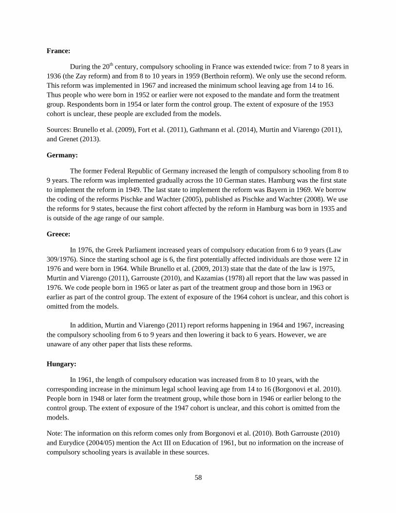
58
France:
During the 20th century, compulsory schooling in France was extended twice: from 7 to 8 years in
1936 (the Zay reform) and from 8 to 10 years in 1959 (Berthoin reform). We only use the second reform.
This reform was implemented in 1967 and increased the minimum school leaving age from 14 to 16.
Thus people who were born in 1952 or earlier were not exposed to the mandate and form the treatment
group. Respondents born in 1954 or later form the control group. The extent of exposure of the 1953
cohort is unclear, these people are excluded from the models.
Sources: Brunello et al. (2009), Fort et al. (2011), Gathmann et al. (2014), Murtin and Viarengo (2011),
and Grenet (2013).
Germany:
The former Federal Republic of Germany increased the length of compulsory schooling from 8 to
9 years. The reform was implemented gradually across the 10 German states. Hamburg was the first state
to implement the reform in 1949. The last state to implement the reform was Bayern in 1969. We borrow
the coding of the reforms Pischke and Wachter (2005), published as Pischke and Wachter (2008). We use
the reforms for 9 states, because the first cohort affected by the reform in Hamburg was born in 1935 and
is outside of the age range of our sample.
Greece:
In 1976, the Greek Parliament increased years of compulsory education from 6 to 9 years (Law
309/1976). Since the starting school age is 6, the first potentially affected individuals are those were 12 in
1976 and were born in 1964. While Brunello et al. (2009, 2013) state that the date of the law is 1975,
Murtin and Viarengo (2011), Garrouste (2010), and Kazamias (1978) all report that the law was passed in
1976. We code people born in 1965 or later as part of the treatment group and those born in 1963 or
earlier as part of the control group. The extent of exposure of the 1964 cohort is unclear, and this cohort is
omitted from the models.
In addition, Murtin and Viarengo (2011) report reforms happening in 1964 and 1967, increasing
the compulsory schooling from 6 to 9 years and then lowering it back to 6 years. However, we are
unaware of any other paper that lists these reforms.
Hungary:
In 1961, the length of compulsory education was increased from 8 to 10 years, with the
corresponding increase in the minimum legal school leaving age from 14 to 16 (Borgonovi et al. 2010).
People born in 1948 or later form the treatment group, while those born in 1946 or earlier belong to the
control group. The extent of exposure of the 1947 cohort is unclear, and this cohort is omitted from the
models.
Note: The information on this reform comes only from Borgonovi et al. (2010). Both Garrouste (2010)
and Eurydice (2004/05) mention the Act III on Education of 1961, but no information on the increase of
compulsory schooling years is available in these sources.

59
Ireland:
In 1972, the minimum school leaving age was increased from 14 to 15. For this reform,
respondents born in 1959 or later form the treatment group, while those born in 1957 or earlier belong to
the control group. The extent of exposure of the 1958 cohort is unclear, and this cohort is omitted from
the models.
According to Brunello et al. (2009), the minimum school leaving age was further increased to 16
in 2000 (the Education (Welfare) Act (2000)). Fort (2006) suggests those born in 1985 as the pivotal
cohort for the second reform. However, Garrouste (2010) mentions that the Education (Welfare) Act of
2000 became operational on July 5th 2002, which would imply that the first potentially affected cohort
was born in 1987. Given the disagreement in literature over the date of implementation of the latest
reform, we only use the 1972 reform.
Sources: Brunello et al. (2009), Fort (2006), Garrouste (2010), Murtin and Viarengo (2011), Gathmann
(2014).
Poland:
In 1961 the length of compulsory education was increased from 7 to 8 years, with the
corresponding increase in the minimum legal school leaving age from 14 to 15 (Borgonovi et al. 2010).
Additional information is provided by the International Education Guide (2012): “Primary school was
extended to 8 years following the introduction of the 1961 Education System Development Act (Ustawa o
rozwoju systemu oswiaty i wychowania). Compulsory education covered Grades 1 to 8 (ages 7 to 15).”
According to Joanna Jung-Miklaszewska (2003), the 8th grade (Form VIII) was organized in the school
year 1966/67. This made those born in 1953 or later to be fully exposed to the reform, while those born in
1951 or earlier missed the mandate. It is uncertain whether the respondents born in 1952 were exposed to
the reform; therefore, this cohort is omitted from the estimations.
Spain:
In 1970, the General Act on Education and Financing of Educational Reform increased years of
compulsory schooling from 6 to 8 and the minimum legal school leaving age from 12 to 14 (Brunello et
al. 2009, Fort 2006, Garrouste 2010, Gathmann et al. 2014). Both Brunello et al. (2009) and Gathmann et
al. (2014) follow Pons and Gonzalo (2002) and code those born in 1957 as the first cohort potentially
affected by the reform. These respondents 13 years old in 1970. We follow this approach and assign
people who were born before 1957 to the control group and people who were born after 1957 to the
treatment group.
The United Kingdom:
In March 1972, the minimum school leaving age was increased from 15 to 16, starting September
1 1972 (www.legislation.gov.uk/uksi/1972/444/pdfs/uksi_19720444_en.pdf). School started at age 5,
which implies that the number of years of compulsory education increased from 10 to 11. In Northern
Ireland, the reform of 1972 also increased the minimum school leaving age from 15 to 16.

60
The mandate affected all individuals born September 1957 or later in England, Wales, and
Northern Ireland. However, the extent of the exposure of the 1957 cohort to the reform in not known.
This cohort is excluded from the analysis. Respondents born in 1958 or later form the treatment group,
while people born in 1956 or earlier form the control group.
For Scotland, several papers report 1976 as the date of the reform (Fort 2006, Gathmann et al.
2014, Brunello et al. 2013). However, Gathmann et al. (2014) and Fort (2006) suggest those born in 1958
as the first potentially affected cohort. We code people born in 1959 as the first fully affected cohort in
Scotland. Those born 1957 or earlier form the control group, while people born in 1958 are excluded from
the models.
In 1940s, the United Kingdom had another education reform that increased the minimum legal
school leaving age from 14 to 15. However, the first cohort exposed to that mandate was born in 1930s. In
order to avoid potentially confounding effects of ageing on religiosity, our sample is restricted to those 65
years old or younger, which prevents the usage of this early reform.
Sources: Brunello et al. (2009), Brunello et al. (2013), Fort (2006), Fort et al. (2011), Murtin and
Viarengo (2011), Clark and Royer (2013), Oreopolous (2006, 2007), Gathmann (2014).
Additional information on education reforms for countries not included the sample:
Czech Republic:
Garrouste (2010) reports several compulsory schooling reforms in Czech Republic in the 20th
century. In 1948, the length of compulsory schooling was increased from 8 years to 9, with the
corresponding change in the minimum school leaving age from 14 to 15. Then the number of compulsory
schooling years was reduced back to 8 years in 1953 and raised again to 9 years in 1960. Furthermore, in
1979, the number of years of compulsory education was reduced to 8, and in 1990 the number was
changed back to 9. Garrouste (2010) also mentions a reform in 1976: “Hence, the reform of 1976 made
secondary education accessible to everybody by instituting 10-year compulsory schooling (8 years at
základní školy and 2 years at střední školy).” The high number of education reforms passed in a relatively
short period makes determining of the reform exposure problematic and the quality of the implementation
questionable. Therefore, Czech Republic is not included in our sample.
Finland:
In 1972-1977, Finland gradually implemented an education reform that increased years of
compulsory schooling from 6 to 9. Both Brunello et al. (2009) and Borgonovi et al. (2010) use this reform
as as a source of identifying variation. However, both Kerr et al. (2013) and Pekkarinen (2008) note that
the reform did not in practice increase the length of compulsory schooling, because the vast majority of
pupils already received 9 years of education. Moreover, Kerr et al. (2013) state that the minimum school
leaving age had been 16 ever since 1957. Because of these remarks, Finland is not included our sample.

61
Italy:
Reform that made junior high school compulsory was passed at the end of 1962 and implemented
in 1963. The mandate increased the years of compulsory schooling from 5 to 8 and minimum legal school
leaving age from 11 to 14. Both Brunello et al. (2009) and Gathmann (2014) refer to Brandolini and
Cipollone (2002) and code those being born in 1949 as the first cohort affected by the reform. This is at
odds with the straightforward calculation 1963-11=1952.
Fort (2006) gives two other cutoffs: “According to [Brandolini and Cipollone, 2002, pp. 12],
people potentially affected by the reform are those who in 1963 were less than 15 years old and without
middle school degree, those who were between 6 and 14 years old in 1963, that is those born between
1949-1957. Instead, [Flabbi, 1999, pp. 13] claimed that the reform starts “to be effective on people born
after the 1950.”
Furthermore, according to Brunello et al. (2009), compliance with the reform was not immediate
and only in 1976 the proportion of children attending junior high school approached 100%.
We do not include Italy in our sample because identifying the first affected cohort is somewhat
problematic and the overall quality of the enforcement of the reform is unclear.
Norway:
Several papers use the educational reform in Norway as a source of identifying variation (Bhuller
et al. 2014, Black et al. 2008, Aakvik et al. 2010, Pelkonen 2012). However, the timing of the reform
implementation differed across municipalities. The data on respondents’ residence at the municipality
level is not available in the ESS, and Norway is not included in the sample. Pelkonen (2012) writes the
following about the reform:
“The reform was launched as an experiment in six municipalities, chosen by the Ministry of
Education, until it was made compulsory by the central government. Once the reform was legislated in
1959, the municipalities were required to implement the reform by the end of 1972, but were given the
liberty to decide the precise timing by themselves. Prior to implementation, local governments were
required to present a plan to the central government on the requirements for new teachers, buildings and
other items the costs of which were to be covered by the central government. Due to these requirements,
the timing of the reform across municipalities depended partly on the interaction between the central
government and the municipalities. Aakvik et al. (2003) also mention that individual school directors may
have been influential in the timing of the reform within municipalities. The reforms were implemented
from 1960 onwards, and the cohorts that were differentially affected by the reform depending on their
place of birth, were born between 1946 and 1961. However, in most of the municipalities, the affected
children were those born between 1947 and 1958. A handful of municipalities appear to have reformed
after the required deadline, affecting those born between 1959–1961, while some municipalities that were
early experimental reformers, started with the cohort born in 1946.”
Portugal:
Portugal experienced several compulsory schooling reforms during the 20th century. First, in
1956, the number of years of compulsory education was increased for boys only from 3 to 4 years. This

62
mandate affected all the boys who entered school in 1956 or later, i.e. those born in 1948 or later (the
school starting age was 8). However, boys who either did not complete 4 years of education or were not
12 in 1956 still were required to go back to school, which means that those born in 1945 were potentially
affected by the reform as well. In 1960, the reform was extended to girls. Second, in 1964, the number of
years of compulsory schooling was further increased from 4 to 6 for both genders, raising the minimum
legal school leaving age to 14. The reform applied to those who entered school from 1964 onwards, i.e.
those born in 1956 and later. Third, in 1973, there was an attempt to increase the years of compulsory
schooling from 6 to 8, but the reform was not fully implemented. Fourth, in 1986, the length of
compulsory education was increased from 6 years to 9. Fort (2006) gives the following, somewhat
confusing, description: “This measure covered children who, once they had completed 6 years of
schooling by 15 September, enrolled in the first year of schooling, as from the 1987/88 school year.”
As in the case of Czech Republic, the high number of education reforms passed in a relatively
short period makes determining of the reform exposure problematic and the quality of the implementation
questionable. Therefore, Portugal is not included in our sample.
Sources: Fort (2006), Garrouste (2010).
Sweden:
In 1962, Sweden increased its years of compulsory schooling from 8 to 9 (Brunello et al. 2009,
Fort 2006, Murtin and Viarengo 2011). However, the full implementation of this reform was preceded by
a period of experimental gradual implementation at the municipality level, which started in 1949.
Brunello et al. (2009) and Borgonovi et al. (2010) code those born in 1950 and 1951 as the
pivotal cohorts, respectively. At the same time Garrouste (2010) states that the law increased years of
compulsory education from 7 (not 8) to 9 and mentions that “…this law got, however, fully implemented
only in 1972.”
Given the lack of clarity for the timing of the reform implementation, we leave Sweden out of our
sample.
Switzerland:
Murtin and Viarengo (2011) are the only source that mentions a reform changing the years of
compulsory schooling in Switzerland. They state that in 1970 the number of years of compulsory
education was increased from 8 to 9. They also point out that 1970 corresponds to the first
implementation of the policy change and that the implementation differed across Swiss Cantons. Since
Murtin and Viarengo (2011) provide no further information on the dates of implementation in different
Swiss Cantons, we do not include Switzerland in our sample.
The Netherlands:
Several compulsory schooling reforms happened in the Netherlands during the 20th century, and
the literature is not always consistent about their timing and details.
Brunello et al. (2009), Gathmann et al. (2014), and Fort (2006) report a 1975 reform that
increased minimum school leaving age by one year, from 15 to 16. At the same time, three-year lower

63
vocational programs were extended to four years. The reform stated that all schools of lower vocational
education should implement a second general year – with at least 20 weekly lessons of general training in
the curriculum. The implementation of the reform started in 1973 – since August 1, 1973, all lower
vocational programs had a length of four years. Students who were in their third year in 1973 could still
graduate in a three-year course in 1974, i.e. students who started a three-year course of lower vocational
education on August 1, 1971. All the following cohorts had to take a four-year course. Students born on
or after August 1, 1959, had 10 years of complete education, with a four-year lower vocational education
course as part of it. Garrouste (2010) reports the reform for the same compulsory schooling increase in
1969 instead of 1975.
This appendix does not describe the reforms that happened earlier than 1940s, readers are referred
to Gathmann et al. (2014) and Garrouste (2010) for the descriptions of education reforms in Netherlands
in early 20th century.
Murtin and Viarengo (2011), Gathmann et al. (2014), and Fort et al. (2011) report an increase in
years of compulsory schooling by two years taking place in 1950.
Fort et al. (2011) reports changes in years of compulsory schooling in 1942 from 7 to 8, then in
1947 from 8 to 7. Garrouste (2010) documents an increase in years of compulsory schooling from 7 to 8
in 1942, which was implemented in 1949.
Then Murtin and Viarengo (2011) report an increase in years of compulsory schooling from 8 to
9 in 1971. Garrouste (2010) attributes the same increase to year 1968.
Garrouste (2010) also reports an increase in compulsory years of schooling from 10 to 11 in
1971: “In 1971, an additional period of part-time compulsory education was added for young people who
had completed their period of full-time compulsory education. Under-18s must attend school at least one
day a week until the end of the school year in which they turn 17.”
Finally, Gathmann (2014), Garrouste (2010), and Murtin and Viarengo (2011) state that in 1985
the Primary Education Act (WBO) of 1981 was implemented, resulting in a change in school starting age.
After the reform compulsory school started the first month after children turned 5 (before the reform the
lower age limit was 6). They had to stay in school until they have attended at least 12 complete years of
schooling and in any case until the end of the school year when they turn 16, after which they were
required to take one year part-time courses.

64
Appendix C. Data
ESS Religious Denominations
Respondents in the ESS were asked whether they belong to a religious denomination and, if so, to
which denomination they belong. Possible answers included 1 “Roman Catholic,” 2 “Protestant,” 3
“Eastern Orthodox,” 4 “Other Christian denomination,” 5 “Jewish,” 6 “Islamic,” 7 “Eastern religions,”
and 8 “Other non-Christian religions.” However, there were inconsistencies in the religious denomination
reporting in the ESS data. First, in Round 2 of the ESS, for Hungarian respondents the category “Eastern
Orthodox” was merged with the category “Roman Catholic.” Second, for respondents from France in
Rounds 1 and 2, the category “Other Christian denomination” was merged with the category “Other non-
Christian religions.” Third, in the United Kingdom in Rounds 2 and 3, many interviewers appear not to
have probed respondents sufficiently if the respondents simply reported their religion as being
“Christian.” Rather than asking for more details about the Christian denomination to which the
respondent felt they belonged, the interviewer instead used the “Other Christian denomination” category.
This resulted in significantly larger proportions of people reporting belonging to “Other Christian
denomination” when compared to other ESS rounds of the United Kingdom data (Rounds 1, 4, 5, and 6).
These inconsistencies prevented the creation of a uniform religious denomination variable with fine
subcategories. The final denomination variable has categories 1 “No denomination,” 2 “Christian,” and 3
“Non-Christian.”
EVS Sample Description
The European Values Study (EVS) consists of four waves of cross-sectional surveys conducted in
49 predominantly European countries in various years from 1981 to 2008.
EVS Superstition Measures:
“Do you believe that a lucky charm such as a mascot or a talisman can protect or help you?”
question was asked in the 1999 wave and the 2008 wave. The possible answers range from 1 “Definitely
not” to 10 “Definitely yes.” For specifications in Table 6, this variable is converted into two dichotomous
indicators taking the values of one if the respondent’s belief in lucky charm is, respectively, greater than
or equal to 4, or greater than or equal to 5. This question was asked in all of the countries already present
in the religiosity analysis. The list of countries in the “lucky charm” sample consists of Austria, Belgium,
Denmark, France, Great Britain, Greece, Hungary, Ireland, Northern Ireland25
, Poland, Spain, and West
Germany.
25
In the EVS data, Northern Ireland enters as a separate country. This is in contrast to the ESS, where originally
Northern Ireland region is treated either as a part of Great Britain (Rounds 1 to 6) or a part of Ireland (Round 4
only). We created a new country “Northern Ireland” in the ESS data when harmonizing the region variable across
rounds. Northern Ireland has a separate country fixed effect in the regressions, but is not present in the graphs, since
the number of observations is small.

65
Two questions about horoscope were asked in the 1999 wave: “How often do you consult your
horoscope to know about your future?”26
and “How often do you take this into account in your daily
life”27
The variable “How often do you consult your horoscope?” is converted into a dummy variable
taking the value of one if the respondent reports consulting with the horoscope at least once a month, and
zero otherwise. Similarly, the variable “How often do you take horoscope into account in daily life?” is
converted into an indicator taking the value of one if the respondent reports taking horoscope into account
at least sometimes, and zero otherwise. The questions about horoscope were asked in four countries, for
which the education reforms information is available: Austria, France, Greece, and West Germany. These
countries compose the “horoscope” sample.
EVS Sample and the Education Measure:
The sample is restricted to individuals younger than 65 years old, citizens of the country of
interview and non-students. In addition, to keep the EVS sample more comparable to the ESS sample,
immigrants were dropped whenever the information on whether the individual was born in the country is
available (the 2008 wave only).
The number of years of education in the ESS is approximated by subtracting the country school
starting age (6 for most countries, 5 for Great Britain and Northern Ireland, 7 for Denmark and Poland)
from the age of education completion as reported by the respondent. Observations for which the current
reported age is less than the reported age of completing education are dropped. In addition, observations
with calculated years of education greater than 25 are dropped as well.
EVS Control Variables:
The information about whether the respondent belongs to country’s dominant nationality group,
parental background information and number of household members is not consistently available across
the waves. Working dummy is equal to one when the respondent reported working full-time and is equal
to zero if the respondent reported being one of the following: working part-time (30 hours or less), self-
employed, retired, housewife/househusband, student, unemployed, other. Married dummy is equal to one
if the respondent is currently legally married and is equal to zero if the respondent reported marital status
as one of the following: cohabiting, divorced, separated, widowed, single/never married. Dummy
childhome indicates whether there is a person under 18 living at home.
Unlike the ESS, the EVS does not ask its respondents about their self-perceived urbanicity.
However, the actual size of the town, in which the interview was conducted, is available starting in the
1990 wave. The possible categories of this variable are “under 2,000,” “2,000-5,000,” “5,000-10,000”
“10,000-20,000,” “20,000-50,000,” “50,000-100,000,” “100,000-500,000,” “500,000+.” Approximately
50% of respondents in the original data lived in towns under 20,000. The variable city takes the value of
one if the size of the town of the interview is 20,000 or more, and zero otherwise.
26The full set of possible answers includes 1 “Every day,” 2 “At least once a week,” 3 “At least once a month,” 4
“Less often,” and 5 “Never.” 27
The full set of possible answers includes 1 “Always,” 2 “Most of the time,” 3 “Sometimes,” 4 “Not very often,”
and 5 “Never.”


