
1
Computation and Causation*
Richard Scheines
Dept. of Philosophy, Carnegie Mellon University
1. Introduction
In 1982, when computers were just becoming widely available, I was a graduate
student beginning my work with Clark Glymour on a PhD thesis entitled: “Causality in
the Social Sciences.” Dazed and confused by the vast philosophical literature on
causation, I found relative solace in the clarity of Structural Equation Models (SEMs), a
form of statistical model used commonly by practicing sociologists, political scientists,
etc., to model causal hypotheses with which associations among measured variables
might be explained. The statistical literature around SEMs was vast as well, but Clark
had extracted from it a particular kind of evidential constraint first studied by Charles
Spearman at the beginning of the 20th
century, the “vanishing tetrad difference.”1 As it
turned out, certain kinds of causal structures entailed these constraints, and others did not.
Spearman used this lever to argue for the existence of a single, general intelligence factor,
the infamous g (Spearman, 1904).
In 1982, we could, with laborious effort, calculate the set of tetrad constraints
entailed by a given SEM. We did not, however, have any general characterization of the
connection between qualitative causal structure, as represented by the “path diagram” for
a SEM (Wright, 1934), and vanishing tetrad constraints. If we could only find such a
characterization, we thought, then we could lay down a method of causal discovery from
statistical data heretofore written off as impossible. Two or three times a week I would
come in to Clark’s office offering a conjecture, which, as is his wont, he would
immediately claim to refute with a complicated counterexample. Although Clark is a
man of astounding vision and amazing intellectual facility, he will never be accused of
* I thank Emily Scheines and Martha Harty for patient reading and wise counsel.
1 A vanishing tetrad difference is an equality among the products of correlations involving an entire
foursome of variables. For example, a vanishing tetrad difference among W, X, Y, Z is wx*yz = wy*xz.
Such a constraint is implied, for example, by a model in which there is a single common cause of W, X, Y,
and Z. In Spearman’s case, tetrad differences among measures of reading and math aptitude led him to
hypothesize that a single common cause, general intelligence, was responsible for performance on all four
pyschometric instruments.
2
being fastidious in calculation, and thus I would dispute his counterexample on the
grounds that he had calculated incorrectly (I had no other advantage on him). We would
then work through the example several times, each time getting a different answer. After
the better part of an hour we would sometimes converge on a calculation we could both
endorse, but the process was so laborious as to make progress on the larger goal almost
hopeless.
Finally, after a particularly long and mind-numbing session, Clark said to me, “why
not write a computer program that would do these calculations for us? The algorithm for
computing the vanishing tetrad difference for a given latent clustering model is clear
enough. You’re young, you can still learn a new trick or two.” Having not the faintest
idea of how many late-night hours I would spend debugging code over the next several
years, I went out and bought a book on Pascal and dove in. Peter Spirtes joined us a few
years later, Kevin Kelly was the first to code the general case in LISP before he went off
to apply formal learning theory to epistemology, and together Clark, Peter and I have
computationally attacked the epistemology of causation for nearly twenty years. By
1984, with the help of the crude program I had written and Kelly’s more elegant one, we
had developed an automatic procedure for correcting a given SEM. By 1987 we had a
graphical characterization of when a SEM entails a vanishing tetrad difference as well as
a different (but related) empirical regularity, the vanishing partial correlation (Glymour,
Scheines, Spirtes, Kelly, 1987). In 1988, because we had become involved in the
artificial intelligence community, we became aware of Judea Pearl’s work in Bayes
Networks. Combining our work on causal discovery, which came from the linear causal
model tradition, with Pearl’s, which came from computer science, produced a perspective
that was much more fertile than the sum of its parts.
In what follows I try to survey this synthesis. To leave the story accessible, I neglect
formality and detail anyplace I can; where I cannot I try to minimize it, and at the end I
point the way to four sources that have all the detail one could want. I begin by sketching
the philosophical perspective on the subject that has dominated discussion for over two
thousand years. I then sketch the work in biological and social science on linear causal
modeling over the last century, which fed directly into my own. I next describe the work
in computer science that took place almost independently of linear causal modeling.
After discussing the synthesis between linear causal modeling and computer science, I
sketch the enormous progress in causal epistemology and algorithmic causal discovery
this synthesis unleashed. I think it is not in the least an overstatement to say that the
computational turn has radically and permanently changed the philosophical,
computational, and statistical view of causation.
3
2. Causal Analysis before the Computer
For nearly two thousand years, the philosophical analysis of causation has
emphasized reducing causal claims, e.g., “A is a cause of B,” to more primitive, or well
understood concepts. In this section I give a whirlwind of these attempts, and try to
convince you that none has succeeded.
Following Hume’s famous regularity theory, J.L. Mackie (1974) gave an account in
which causes are INUS conditions for their effect, that is, Insufficient but Necessary parts
of Unnecessary but Sufficient sets of conditions. Although logical relations are clear
enough, they are not up to the task of capturing even simple features of causation without
excessive ad hocery, for example the asymmetry of causation, or the distinction between
direct and indirect causation.
Hume and Mackie also gave an analysis of causation in terms of counterfactuals, but
the most systematic and sophisticated counterfactual theory of causation is from David
Lewis (1973). Event A was a cause of event B if, according to Lewis, A occurred, B
occurred, and there is no possible world in which A does not occur but B does that is
closer to the actual world than one in which A does not occur and B does not occur
either. Building a semantics for causation on top of similarity metrics over possible
worlds is a dubious enterprise, but even if one likes possible worlds it seems clear that
Lewis has it backwards. We make judgments about what possible worlds are more or
less similar to the one we inhabit on the basis of our beliefs about causal laws, not the
other way around. Causal claims support counterfactual ones, but not vice versa.
Further, Lewis attempted to capture the asymmetry of causation with “miracles,” but the
attempt fails.
Philosophers have also tried to reduce causal relations to probabilistic ones. In
Patrick Suppes’ (1970) theory, A is a prima facie cause of B if A occurs before B in time,
and A and B are associated. Variables A and B are probabilistically dependent, if for
some value b of B, P(A) P(A | B = b). We notate independence between variables A
and B as: A _||_ B, and association as A _||_ B. A is a genuine cause of B if A is a prima
facie cause of B, and there is no event C prior to A such that A and B are independent
conditional on C, i.e., A _||_ B | C.
First, why probability should be considered less mysterious than causation is a
mystery to me. Second, this theory has us quantify over all possible events C prior to A,
a requirement that makes the epistemology of the subject hopeless. Third, the
probabilistic theory requires temporal knowledge. Fourth, the theory rules out cases in
which A is a cause of an intermediary I, I is a cause of B, A is also a direct cause of B,
but the influence of A on B through I is opposite in sign and of exactly the same strength
as that of A on B directly, leaving A and B independent and thus apparently not a cause
of B according to this and other theories like it.
4
_
+
+
Tax Rate
Economic
Activity
Tax
Revenues
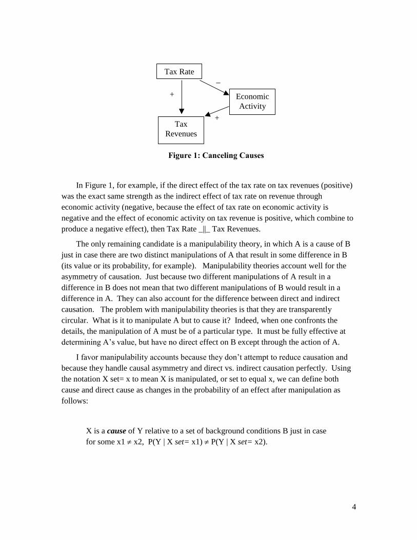
Figure 1: Canceling Causes
In Figure 1, for example, if the direct effect of the tax rate on tax revenues (positive)
was the exact same strength as the indirect effect of tax rate on revenue through
economic activity (negative, because the effect of tax rate on economic activity is
negative and the effect of economic activity on tax revenue is positive, which combine to
produce a negative effect), then Tax Rate _||_ Tax Revenues.
The only remaining candidate is a manipulability theory, in which A is a cause of B
just in case there are two distinct manipulations of A that result in some difference in B
(its value or its probability, for example). Manipulability theories account well for the
asymmetry of causation. Just because two different manipulations of A result in a
difference in B does not mean that two different manipulations of B would result in a
difference in A. They can also account for the difference between direct and indirect
causation. The problem with manipulability theories is that they are transparently
circular. What is it to manipulate A but to cause it? Indeed, when one confronts the
details, the manipulation of A must be of a particular type. It must be fully effective at
determining A’s value, but have no direct effect on B except through the action of A.
I favor manipulability accounts because they don’t attempt to reduce causation and
because they handle causal asymmetry and direct vs. indirect causation perfectly. Using
the notation X set= x to mean X is manipulated, or set to equal x, we can define both
cause and direct cause as changes in the probability of an effect after manipulation as
follows:
X is a cause of Y relative to a set of background conditions B just in case
for some x1 x2, P(Y | X set= x1) P(Y | X set= x2).
5
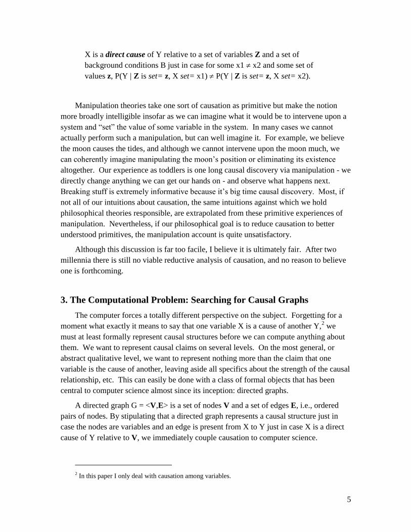
X is a direct cause of Y relative to a set of variables Z and a set of
background conditions B just in case for some x1 x2 and some set of
values z, P(Y | Z is set= z, X set= x1) P(Y | Z is set= z, X set= x2).
Manipulation theories take one sort of causation as primitive but make the notion
more broadly intelligible insofar as we can imagine what it would be to intervene upon a
system and “set” the value of some variable in the system. In many cases we cannot
actually perform such a manipulation, but can well imagine it. For example, we believe
the moon causes the tides, and although we cannot intervene upon the moon much, we
can coherently imagine manipulating the moon’s position or eliminating its existence
altogether. Our experience as toddlers is one long causal discovery via manipulation - we
directly change anything we can get our hands on - and observe what happens next.
Breaking stuff is extremely informative because it’s big time causal discovery. Most, if
not all of our intuitions about causation, the same intuitions against which we hold
philosophical theories responsible, are extrapolated from these primitive experiences of
manipulation. Nevertheless, if our philosophical goal is to reduce causation to better
understood primitives, the manipulation account is quite unsatisfactory.
Although this discussion is far too facile, I believe it is ultimately fair. After two
millennia there is still no viable reductive analysis of causation, and no reason to believe
one is forthcoming.
3. The Computational Problem: Searching for Causal Graphs
The computer forces a totally different perspective on the subject. Forgetting for a
moment what exactly it means to say that one variable X is a cause of another Y,2 we
must at least formally represent causal structures before we can compute anything about
them. We want to represent causal claims on several levels. On the most general, or
abstract qualitative level, we want to represent nothing more than the claim that one
variable is the cause of another, leaving aside all specifics about the strength of the causal
relationship, etc. This can easily be done with a class of formal objects that has been
central to computer science almost since its inception: directed graphs.
A directed graph G = <V,E> is a set of nodes V and a set of edges E, i.e., ordered
pairs of nodes. By stipulating that a directed graph represents a causal structure just in
case the nodes are variables and an edge is present from X to Y just in case X is a direct
cause of Y relative to V, we immediately couple causation to computer science.
2 In this paper I only deal with causation among variables.
6
Two problems come to the fore. One, how does a causal graph, without any further
quantitative elaboration, connect with empirical evidence? That is, what sorts of
evidence does causal structure alone explain? What set of predictions might one causal
graph make and another not, allowing us to distinguish between them? When are two
models empirically indistinguishable? Two, are there efficient methods for searching for
the graph or graphs that explain a given body of evidence? Exactly what assumptions
must such techniques rely upon? Can such methods succeed even when some variables
are left unmeasured?
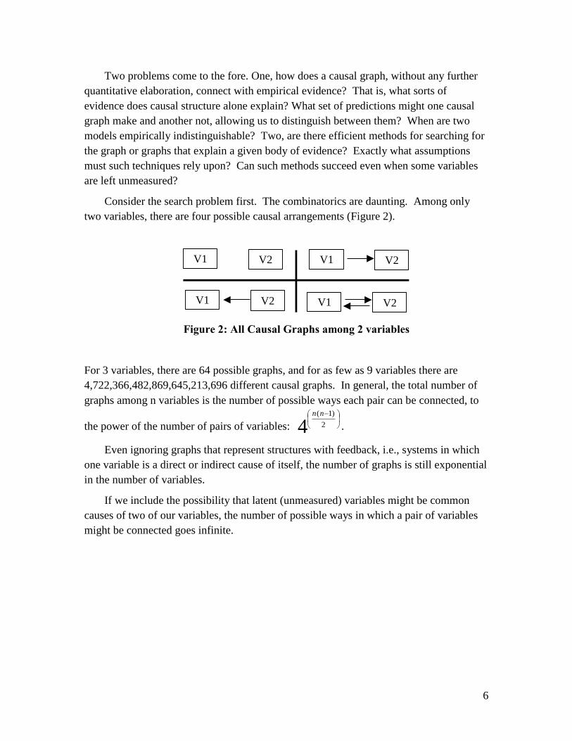
Consider the search problem first. The combinatorics are daunting. Among only
two variables, there are four possible causal arrangements (Figure 2).
V1 V2
V1 V2 V1 V2
V1 V2
Figure 2: All Causal Graphs among 2 variables
For 3 variables, there are 64 possible graphs, and for as few as 9 variables there are
4,722,366,482,869,645,213,696 different causal graphs. In general, the total number of
graphs among n variables is the number of possible ways each pair can be connected, to
the power of the number of pairs of variables: 4 2
)1(
nn
.
Even ignoring graphs that represent structures with feedback, i.e., systems in which
one variable is a direct or indirect cause of itself, the number of graphs is still exponential
in the number of variables.
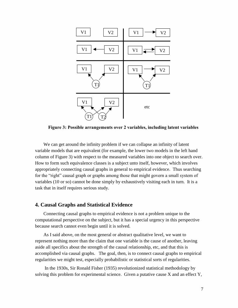
If we include the possibility that latent (unmeasured) variables might be common
causes of two of our variables, the number of possible ways in which a pair of variables
might be connected goes infinite.
7
V1 V2
V1 V2 V1 V2
V1 V2
V1 V2 V1 V2
T1 T1
V1 V2
T2 T1
etc
Figure 3: Possible arrangements over 2 variables, including latent variables
We can get around the infinity problem if we can collapse an infinity of latent
variable models that are equivalent (for example, the lower two models in the left hand
column of Figure 3) with respect to the measured variables into one object to search over.
How to form such equivalence classes is a subject unto itself, however, which involves
appropriately connecting causal graphs in general to empirical evidence. Thus searching
for the “right” causal graph or graphs among those that might govern a small system of
variables (10 or so) cannot be done simply by exhaustively visiting each in turn. It is a
task that in itself requires serious study.
4. Causal Graphs and Statistical Evidence
Connecting causal graphs to empirical evidence is not a problem unique to the
computational perspective on the subject, but it has a special urgency in this perspective
because search cannot even begin until it is solved.
As I said above, on the most general or abstract qualitative level, we want to
represent nothing more than the claim that one variable is the cause of another, leaving
aside all specifics about the strength of the causal relationship, etc, and that this is
accomplished via causal graphs. The goal, then, is to connect causal graphs to empirical
regularities we might test, especially probabilistic or statistical sorts of regularities.
In the 1930s, Sir Ronald Fisher (1935) revolutionized statistical methodology by
solving this problem for experimental science. Given a putative cause X and an effect Y,
8
Fisher provided a detailed method for statistically testing whether X is a cause (direct or
indirect) of Y. His test involved two pieces. One was instructions on how to randomly
assign the value of X for different individuals in the experiment, and the other was
instructions for how to compute a “null distribution” against which to compare the
outcome of the experiment, i.e., the possible outcomes and their expected relative
frequencies if X has no effect whatsoever on Y. Although this was an amazing
breakthrough, and still constitutes the methodological core of what the FDA requires of
studies aimed at establishing the causal effect of some drug or new medical procedure, it
requires that one can manipulate (set) the value of the putative cause X. In lots of
contexts, one cannot achieve this level of control for ethical or practical reasons. For
example, in investigating whether the HIV virus is truly the cause of AIDs in humans, we
cannot randomly assign some group to “treatment” and infect them with HIV.
The real problem, then, is connecting causal graphs to empirical evidence in non-
experimental settings.
4.1 Linear Models
From the late 19th
century until very recently, statisticians and social scientists
represented causal models not as qualitative directed graphs, but rather as parametric
models, usually as systems of linear equations. In such models, the empirical
regularities explained are correlations, the measure of linear association quantified by
Karl Pearson. Working at the turn of the 20th
century, for example, Charles Spearman
used linear models to model general intelligence. Biologist Sewall Wright (1934),
writing a few decades later, invented “path analysis,” the forerunner of SEMs. This
tradition continued with Herb Simon’s (1953) pioneering work on causal ordering in
economics, Blalock’s (1961) work in sociology, Costner’s (1971) work in sociology and
political science, Heise’s (1975) work in social science generally, and Karl Joreskog’s
work in psychometrics (1973). Causal modeling with linear parametric systems is still
the standard in the Structural Equation Model world (Bollen, 1989).
In such parametric systems, effects are expressed as linear functions of their direct
causes, plus “noise.” For example, a system expressing the effects of Lead and
Socioeconomic status (measured as a continuous variable between –10 and +10, for
example) on a child’s IQ might be represented as follows:
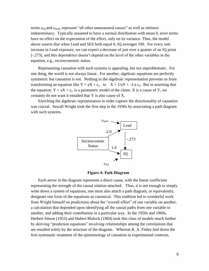
1) IQ = 100 - .273*Lead + 1.0*SES +IQ
2) Lead = 10 - 2.0*SES + lead
The linear coefficients represent the dependence of the left hand side variable’s
expectation on the value of non-error variables on the right hand side. The noise or error
9
terms IQ and lead, represent “all other unmeasured causes” as well as intrinsic
indeterminacy. Typically assumed to have a normal distribution with mean 0, error terms
have no effect on the expectation of the effect, only on its variance. Thus, the model
above asserts that when Lead and SES both equal 0, IQ averages 100. For every unit
increase in Lead exposure, we can expect a decrease of just over a quarter of an IQ point
(-.273), and this dependence doesn’t depend on the level of the other variables in the
equation, e.g., socioeconomic status.
Representing causation with such systems is appealing, but not unproblematic. For
one thing, the world is not always linear. For another, algebraic equations are perfectly
symmetric but causation is not. Nothing in the algebraic representation prevents us from
transforming an equation like Y = aX + y to X = 1/aY + -1/a y. But in asserting that
the equation: Y = aX + y is a parametric model of the claim: X is a cause of Y, we
certainly do not want it entailed that Y is also cause of X.
Enriching the algebraic representation in order capture the directionality of causation
was crucial. Sewall Wright took the first step in the 1930s by associating a path diagram
with such systems.
1.0
Socioeconmic
Status
-.273
-2.0
Lead
IQ
IQ
lead
Figure 4: Path Diagram
Each arrow in the diagram represents a direct cause, with the linear coefficient
representing the strength of the causal relation attached. Thus, it is not enough to simply
write down a system of equations, one must also attach a path diagram, or equivalently,
designate one form of the equations as canonical. This tradition led to wonderful work
from Wright himself on predictions about the “overall effect” of one variable on another,
a calculation that depended upon identifying all the causal paths from one variable to
another, and adding their contribution in a particular way. In the 1950s and 1960s,
Herbert Simon (1953) and Hubert Blalock (1964) took this class of models much further
by deriving “prediction equations” involving relationships among the correlations that
are entailed solely by the structure of the diagram. Whereas R. A. Fisher laid down the
first systematic treatment of the epistemology of causation in experimental contexts,
10
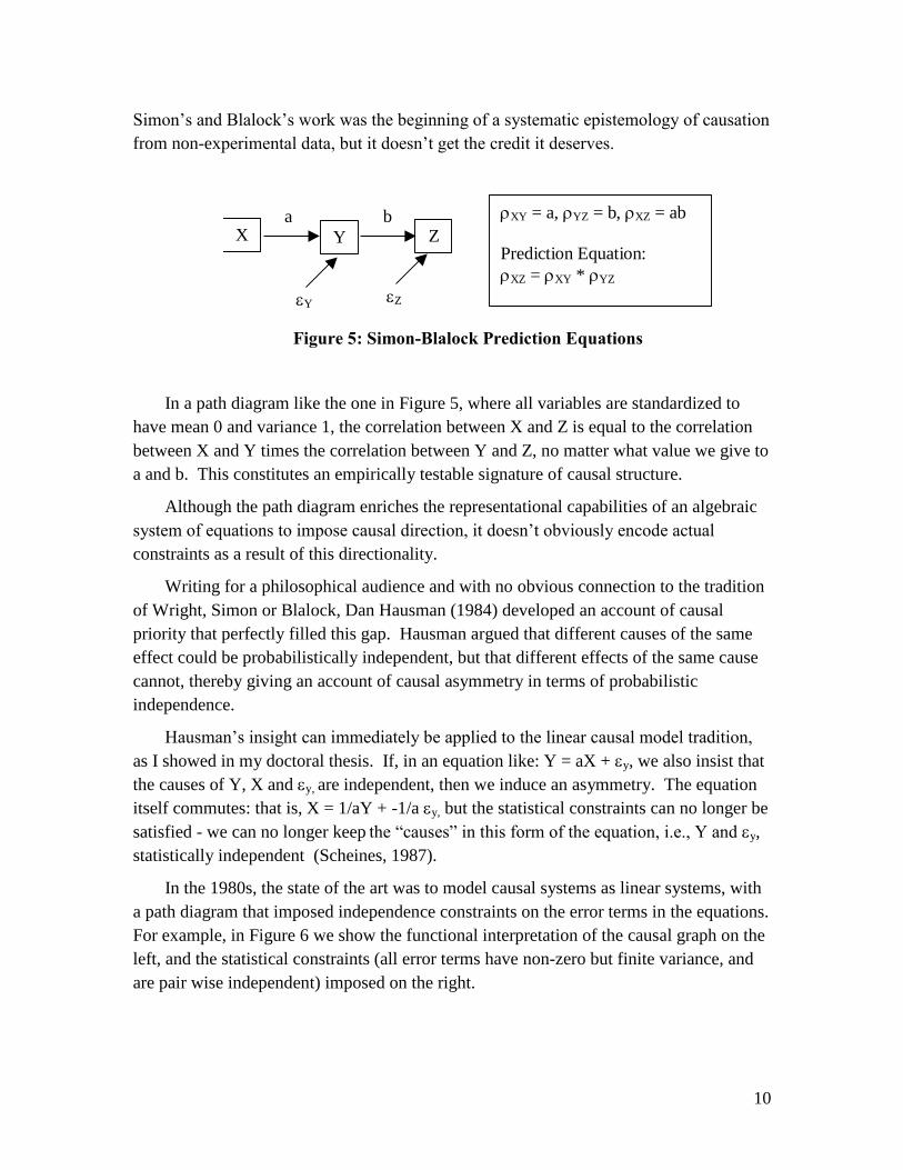
Simon’s and Blalock’s work was the beginning of a systematic epistemology of causation
from non-experimental data, but it doesn’t get the credit it deserves.
a
Y
X Y Z b
Z
XY = a, YZ = b, XZ = ab
Prediction Equation:
XZ = XY * YZ
Figure 5: Simon-Blalock Prediction Equations
In a path diagram like the one in Figure 5, where all variables are standardized to
have mean 0 and variance 1, the correlation between X and Z is equal to the correlation
between X and Y times the correlation between Y and Z, no matter what value we give to
a and b. This constitutes an empirically testable signature of causal structure.
Although the path diagram enriches the representational capabilities of an algebraic
system of equations to impose causal direction, it doesn’t obviously encode actual
constraints as a result of this directionality.
Writing for a philosophical audience and with no obvious connection to the tradition
of Wright, Simon or Blalock, Dan Hausman (1984) developed an account of causal
priority that perfectly filled this gap. Hausman argued that different causes of the same
effect could be probabilistically independent, but that different effects of the same cause
cannot, thereby giving an account of causal asymmetry in terms of probabilistic
independence.
Hausman’s insight can immediately be applied to the linear causal model tradition,
as I showed in my doctoral thesis. If, in an equation like: Y = aX + y, we also insist that
the causes of Y, X and y, are independent, then we induce an asymmetry. The equation
itself commutes: that is, X = 1/aY + -1/a y, but the statistical constraints can no longer be
satisfied - we can no longer keep the “causes” in this form of the equation, i.e., Y and y,
statistically independent (Scheines, 1987).
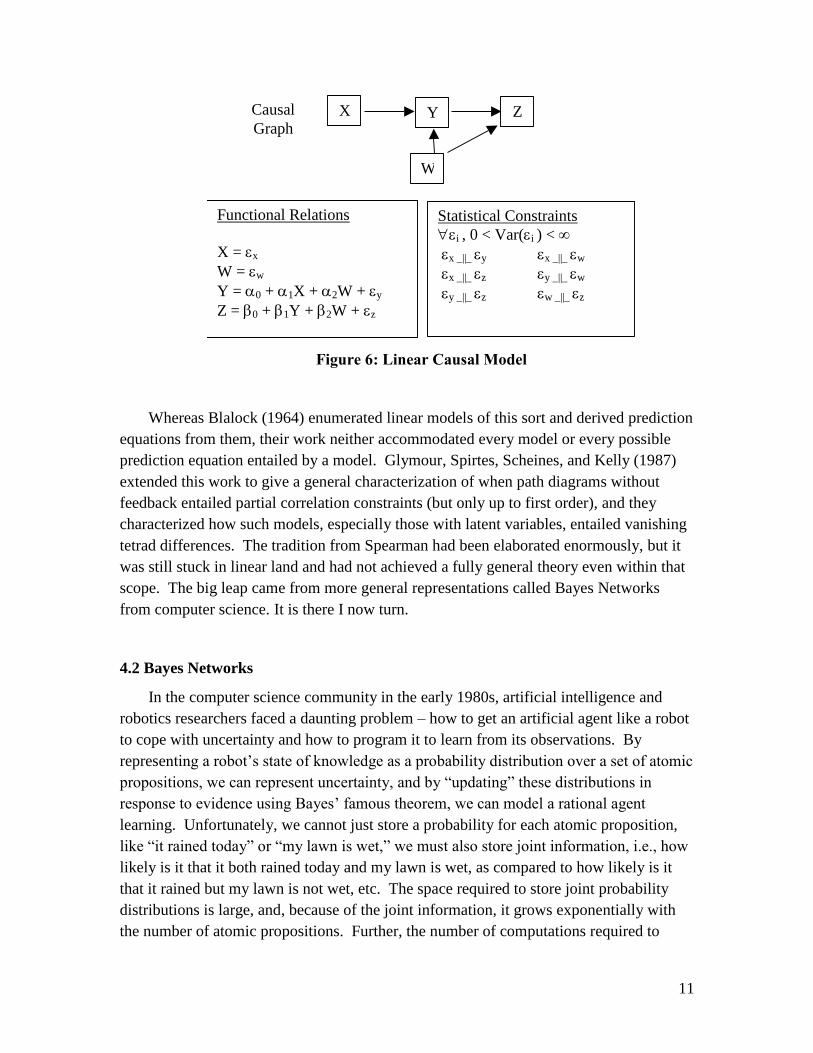
In the 1980s, the state of the art was to model causal systems as linear systems, with
a path diagram that imposed independence constraints on the error terms in the equations.
For example, in Figure 6 we show the functional interpretation of the causal graph on the
left, and the statistical constraints (all error terms have non-zero but finite variance, and
are pair wise independent) imposed on the right.
11
X Y Z
Functional Relations
X = x
W = w
Y = 0 + 1X + 2W + y
Z = 0 + 1Y + 2W + z
W
Statistical Constraints
i , 0 < Var(i ) <
x _||_ y x _||_ w
x _||_ z y _||_ w
y _||_ z w _||_ z
Causal
Graph
Figure 6: Linear Causal Model
Whereas Blalock (1964) enumerated linear models of this sort and derived prediction
equations from them, their work neither accommodated every model or every possible
prediction equation entailed by a model. Glymour, Spirtes, Scheines, and Kelly (1987)
extended this work to give a general characterization of when path diagrams without
feedback entailed partial correlation constraints (but only up to first order), and they
characterized how such models, especially those with latent variables, entailed vanishing
tetrad differences. The tradition from Spearman had been elaborated enormously, but it
was still stuck in linear land and had not achieved a fully general theory even within that
scope. The big leap came from more general representations called Bayes Networks
from computer science. It is there I now turn.
4.2 Bayes Networks
In the computer science community in the early 1980s, artificial intelligence and
robotics researchers faced a daunting problem – how to get an artificial agent like a robot
to cope with uncertainty and how to program it to learn from its observations. By
representing a robot’s state of knowledge as a probability distribution over a set of atomic
propositions, we can represent uncertainty, and by “updating” these distributions in
response to evidence using Bayes’ famous theorem, we can model a rational agent
learning. Unfortunately, we cannot just store a probability for each atomic proposition,
like “it rained today” or “my lawn is wet,” we must also store joint information, i.e., how
likely is it that it both rained today and my lawn is wet, as compared to how likely is it
that it rained but my lawn is not wet, etc. The space required to store joint probability
distributions is large, and, because of the joint information, it grows exponentially with
the number of atomic propositions. Further, the number of computations required to
12
update a joint probability distribution, if done naively, is prohibitive. Again, this task
grows exponentially with the number of atoms in the algebra.
Fortunately, these are just the sorts of problems computer scientists eat for lunch.
Some realized that propositions are often independent. For example, learning that it
rained today is quite informative about whether your lawn is wet, but not in the least
informative about whether your phone is off the hook. By taking advantage of such
independencies, the space required to store the joint distribution and the number of
computations required for updating can be decreased dramatically. Others figured out
that directed graphs could encode the independence relationships true of the atomic
propositions, and that such graphs could themselves be used to figure out very efficiently
exactly how to update the robot’s overall knowledge when new evidence came in
(Lauritzen and Spiegelhalter, 1988).
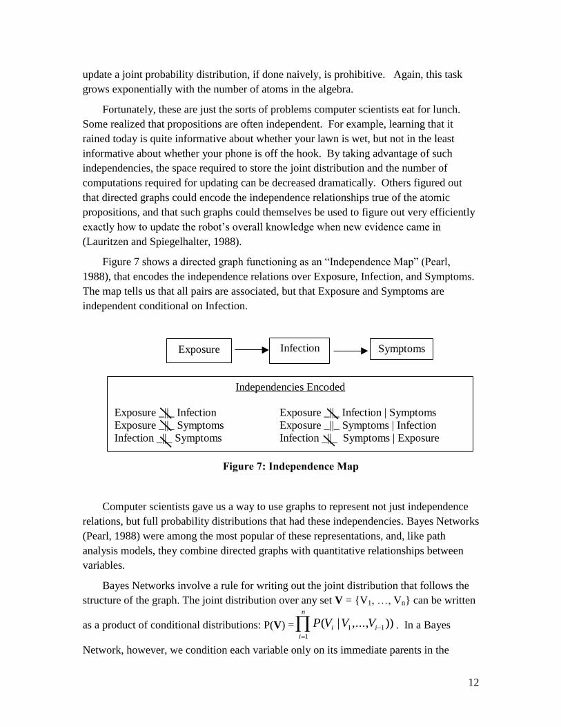
Figure 7 shows a directed graph functioning as an “Independence Map” (Pearl,
1988), that encodes the independence relations over Exposure, Infection, and Symptoms.
The map tells us that all pairs are associated, but that Exposure and Symptoms are
independent conditional on Infection.
Exposure Infection Symptoms
Independencies Encoded
Exposure _||_ Infection Exposure _||_ Infection | Symptoms
Exposure _||_ Symptoms Exposure _||_ Symptoms | Infection
Infection _||_ Symptoms Infection _||_ Symptoms | Exposure
Figure 7: Independence Map
Computer scientists gave us a way to use graphs to represent not just independence
relations, but full probability distributions that had these independencies. Bayes Networks
(Pearl, 1988) were among the most popular of these representations, and, like path
analysis models, they combine directed graphs with quantitative relationships between
variables.
Bayes Networks involve a rule for writing out the joint distribution that follows the
structure of the graph. The joint distribution over any set V = {V1, …, Vn} can be written
as a product of conditional distributions: P(V) =
n
i
ii VVVP1
11 )),...,|( . In a Bayes
Network, however, we condition each variable only on its immediate parents in the
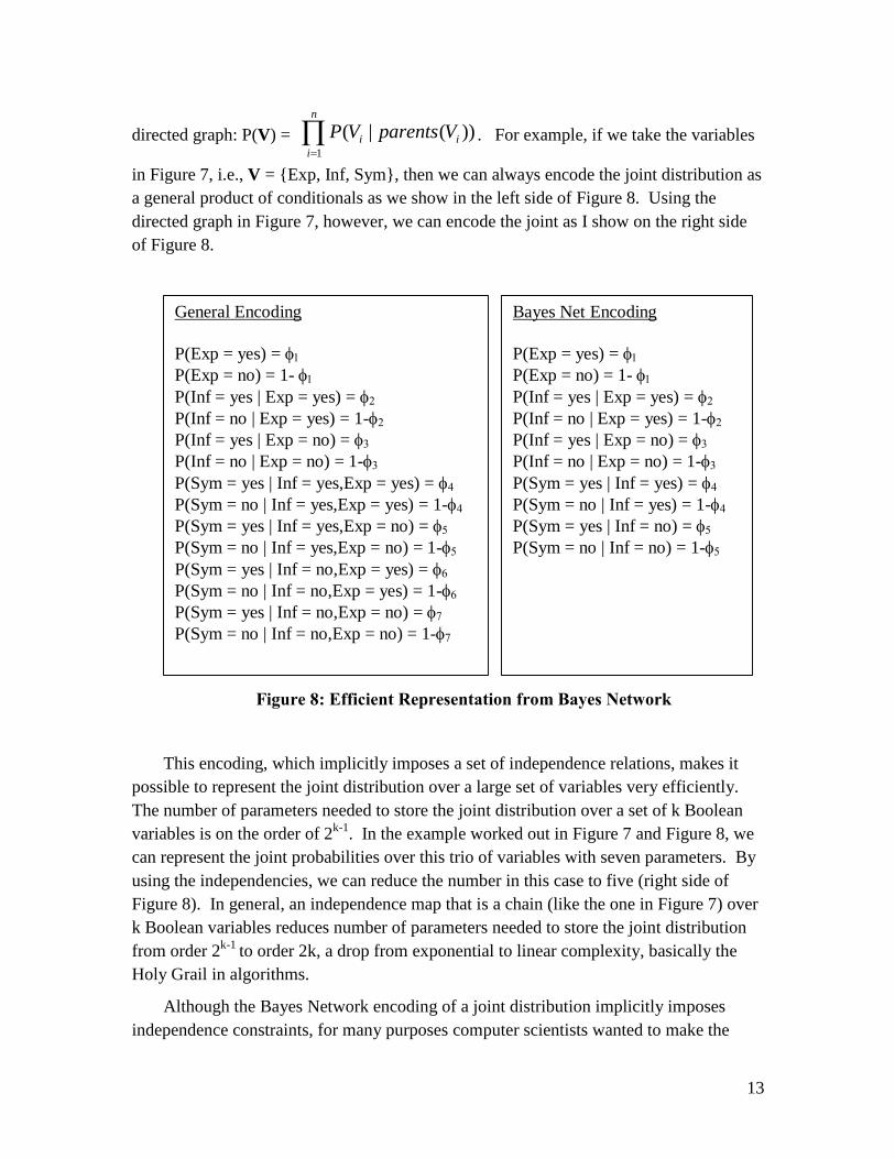
13
directed graph: P(V) =
n
i
ii VparentsVP1
))(|( . For example, if we take the variables
in Figure 7, i.e., V = {Exp, Inf, Sym}, then we can always encode the joint distribution as
a general product of conditionals as we show in the left side of Figure 8. Using the
directed graph in Figure 7, however, we can encode the joint as I show on the right side
of Figure 8.
General Encoding
P(Exp = yes) =
P(Exp = no) = 1- P(Inf = yes | Exp = yes) =
P(Inf = no | Exp = yes) = 1-
P(Inf = yes | Exp = no) =
P(Inf = no | Exp = no) = 1-P(Sym = yes | Inf = yes,Exp = yes) =
P(Sym = no | Inf = yes,Exp = yes) = 1-P(Sym = yes | Inf = yes,Exp = no) = P(Sym = no | Inf = yes,Exp = no) = 1-P(Sym = yes | Inf = no,Exp = yes) =
P(Sym = no | Inf = no,Exp = yes) = 1-P(Sym = yes | Inf = no,Exp = no) = P(Sym = no | Inf = no,Exp = no) = 1-
Bayes Net Encoding
P(Exp = yes) =
P(Exp = no) = 1- P(Inf = yes | Exp = yes) =
P(Inf = no | Exp = yes) = 1-
P(Inf = yes | Exp = no) =
P(Inf = no | Exp = no) = 1-P(Sym = yes | Inf = yes) =
P(Sym = no | Inf = yes) = 1-P(Sym = yes | Inf = no) =
P(Sym = no | Inf = no) = 1-
Figure 8: Efficient Representation from Bayes Network
This encoding, which implicitly imposes a set of independence relations, makes it
possible to represent the joint distribution over a large set of variables very efficiently.
The number of parameters needed to store the joint distribution over a set of k Boolean
variables is on the order of 2k-1
. In the example worked out in Figure 7 and Figure 8, we
can represent the joint probabilities over this trio of variables with seven parameters. By
using the independencies, we can reduce the number in this case to five (right side of
Figure 8). In general, an independence map that is a chain (like the one in Figure 7) over
k Boolean variables reduces number of parameters needed to store the joint distribution
from order 2k-1
to order 2k, a drop from exponential to linear complexity, basically the
Holy Grail in algorithms.
Although the Bayes Network encoding of a joint distribution implicitly imposes
independence constraints, for many purposes computer scientists wanted to make the
14
independencies entailed explicit. Ideally, they wanted a way to simply read the
independencies entailed by a Bayes Network encoding off of the directed graph, without
having to bother with the probability tables at all. Judea Pearl (1988) and some of his
students at UCLA solved this problem in the middle of the 1980s, and they called their
solution d-separation, which stands for dependence-separation.
D-separation provides a graphical definition for determining when a set of variables
X are d-separated from another set Y by a set Z in a causal graph.3 Pearl and his student
Thomas Verma proved that, in a Bayes Network, if a set of variables X are d-separated
from another set Y by a set Z in the directed graph of the network, then X _||_ Y | Z in
every joint distribution representable by that Bayes Network.
4.3 Causal Bayes Networks
Toiling away in the land of linear causal models, my group became aware of Bayes
Networks and d-separation around 1988. We soon realized that the linear causal models
we had been studying were a special kind of Bayes Network, but a Bayes Network just
the same. It immediately became apparent that d-separation provided the general link
between causal structure and empirical regularity we had been looking for.
What needed to happen, however, is that the edges in the directed graphs associated
with Bayes Networks had to be interpreted as representing direct causation. Even if one
could attach such an interpretation to linear causal models, the question was, why do so
generally?
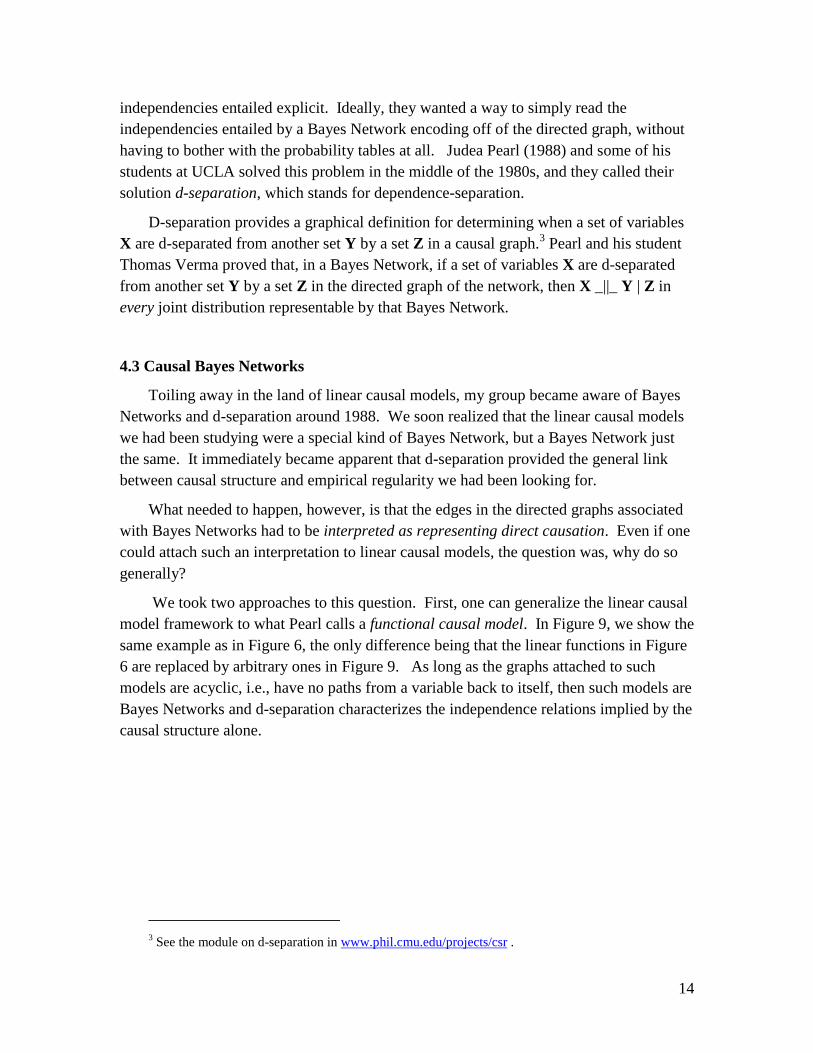
We took two approaches to this question. First, one can generalize the linear causal
model framework to what Pearl calls a functional causal model. In Figure 9, we show the
same example as in Figure 6, the only difference being that the linear functions in Figure
6 are replaced by arbitrary ones in Figure 9. As long as the graphs attached to such
models are acyclic, i.e., have no paths from a variable back to itself, then such models are
Bayes Networks and d-separation characterizes the independence relations implied by the
causal structure alone.
3 See the module on d-separation in www.phil.cmu.edu/projects/csr .
15
X Y Z
Functional Relations
X = x
W = w
Y = fX,W) + y
Z = gY,W) + z
W
Statistical Constraints
i , 0 < Var(i ) <
x _||_ y x _||_ w
x _||_ z y _||_ w
y _||_ z w _||_ z
Causal
Graph
Figure 9: Functional Causal Model
Second, one can formulate axioms that make explicit the assumptions required to
connect causal structure to probabilistic independence in a way equivalent to a Bayes
Network. This approach resulted in the Causal Markov Axiom (Spirtes, Glymour,
Scheines, 1993, chap. 3), which can be stated as follows.
A causal graph G over a set of variables V satisfies the Causal Markov
Axiom just in case in every probability distribution P(V) that G can
produce, each V V is independent of all other variables in V besides V’s
effects, conditional on V’s direct causes.
This axiom is constructed from two intuitions, one from Markov and one from
philosophers Hans Reichenbach (1956) and Wes Salmon (1980). In Markov processes,
future states are independent of past states given current states. Put another way,
variables are independent of their indirect causes given their direct causes. Reichenbach
and Salmon discussed how a common cause “screens off” its effects, the upshot being
that two variables not directly causally related are independent conditional on all of their
common causes.
Causal structures with no feedback that satisfy the Causal Markov Axiom also
satisfy d-separation. Interestingly, linear causal models with feedback do not satisfy the
Causal Markov Axiom, but they do satisfy d-separation.
By the early 1990s it was clear that the computer science community and the
philosophical community had teamed up to produce a plausible and quite general account
of how causal structure alone connected to empirical regularity. What was left was to
16
sketch 1) how to model the use of causal knowledge to predict the effect of interventions,
and 2) how to automatically search for causal models from data with the computer.
5. Causal Prediction: Modeling Manipulations
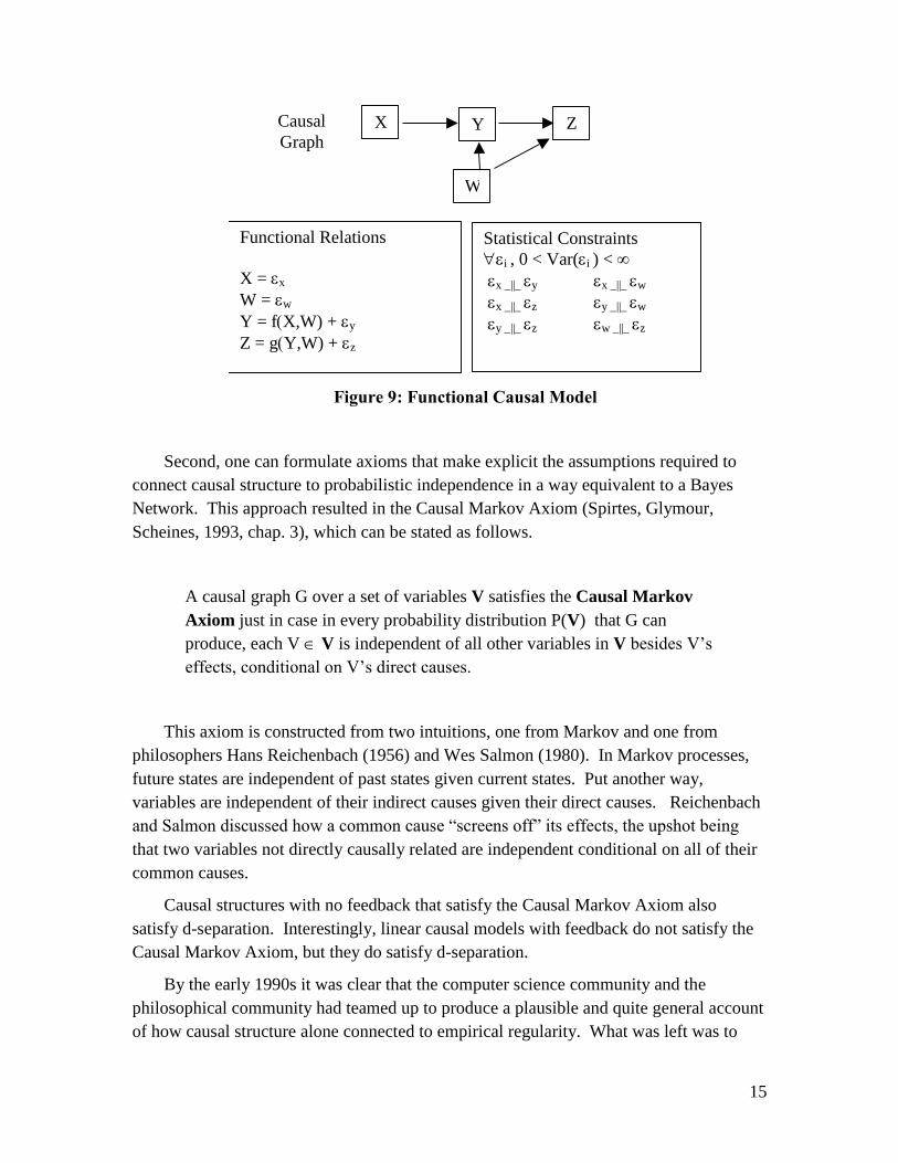
One clear benefit of having causal knowledge is being able to predict the effect of a
manipulation or intervention. For example, smoking and getting lung cancer are
positively associated, as are having tar-stained fingers and getting lung cancer. Since it is
extremely difficult to induce people to stop smoking, perhaps a better public policy to
combat lung cancer is to provide people with good tar-solvent soap and advise them to
scrub the stains off their fingers every day. How do we know this policy is a joke? We
know because we have a causal theory that tells us how the system would respond to our
tar-solvent soap intervention.
Tar-stained
fingers
Smokes
Lung Cancer
Causal Graph
before intervention
Tar-stained
fingers
Smokes
Lung Cancer
Causal Graph
after intervention
Tar-solvent
soap
Figure 10: Intervention
The soap-intervention seizes all influence over the Tar-stained Fingers variable,
and we model this by “x-ing” out the edge from Smokes to Tar-stained Fingers. In the
resulting structure, Tar-Stained Fingers and Lung Cancer are no longer even associated.
The simple way to model an intervention on a causal graph, which we first
articulated coherently in 19894 but which was anticipated by Haavelmo as far back as
4 Reprinted as chapter 2 in (Glymour and Cooper, 1999).
17
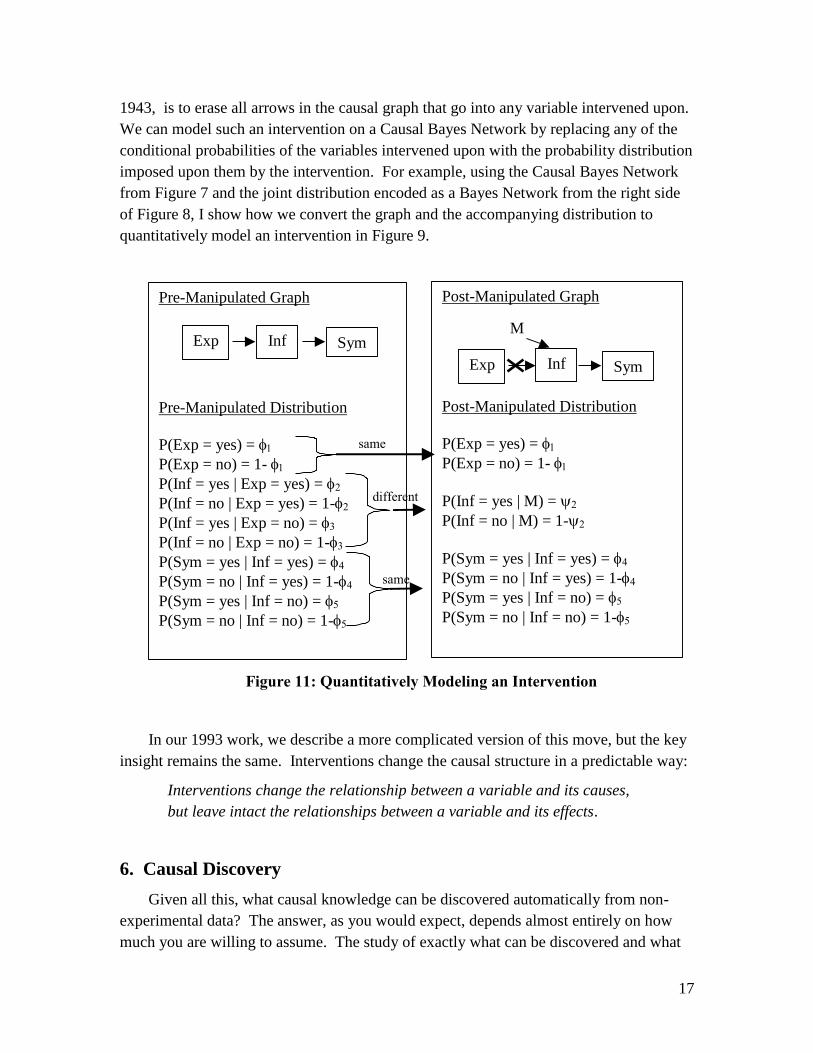
1943, is to erase all arrows in the causal graph that go into any variable intervened upon.
We can model such an intervention on a Causal Bayes Network by replacing any of the
conditional probabilities of the variables intervened upon with the probability distribution
imposed upon them by the intervention. For example, using the Causal Bayes Network
from Figure 7 and the joint distribution encoded as a Bayes Network from the right side
of Figure 8, I show how we convert the graph and the accompanying distribution to
quantitatively model an intervention in Figure 9.
Exp Inf Sym
M
Post-Manipulated Graph
Post-Manipulated Distribution
P(Exp = yes) =
P(Exp = no) = 1-
P(Inf = yes | M) =
P(Inf = no | M) = 1-
P(Sym = yes | Inf = yes) =
P(Sym = no | Inf = yes) = 1-P(Sym = yes | Inf = no) =
P(Sym = no | Inf = no) = 1-
Exp Inf Sym
same
Pre-Manipulated Graph
Pre-Manipulated Distribution
P(Exp = yes) =
P(Exp = no) = 1- P(Inf = yes | Exp = yes) =
P(Inf = no | Exp = yes) = 1-
P(Inf = yes | Exp = no) =
P(Inf = no | Exp = no) = 1-P(Sym = yes | Inf = yes) =
P(Sym = no | Inf = yes) = 1-P(Sym = yes | Inf = no) =
P(Sym = no | Inf = no) = 1-
different
same
Figure 11: Quantitatively Modeling an Intervention
In our 1993 work, we describe a more complicated version of this move, but the key
insight remains the same. Interventions change the causal structure in a predictable way:
Interventions change the relationship between a variable and its causes,
but leave intact the relationships between a variable and its effects.
6. Causal Discovery
Given all this, what causal knowledge can be discovered automatically from non-
experimental data? The answer, as you would expect, depends almost entirely on how
much you are willing to assume. The study of exactly what can be discovered and what
18
cannot under what assumptions has become what I call the computational epistemology
of causal science.
What sorts of assumptions am I referring to? Assumptions such as the Causal
Markov Axiom, the assumption that no feedback exists, and the assumption that no latent
common causes are active. If one is not even willing to assume the Causal Markov
Axiom, or something like it, the game cannot even begin. Even if one is willing to
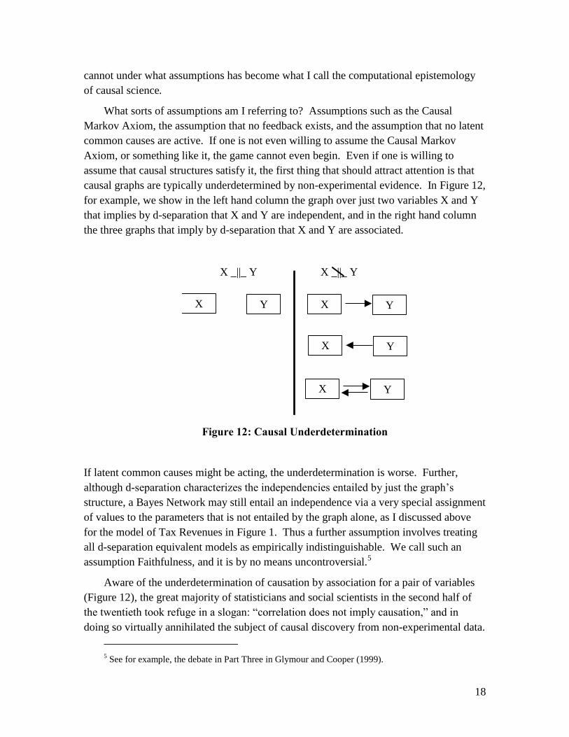
assume that causal structures satisfy it, the first thing that should attract attention is that
causal graphs are typically underdetermined by non-experimental evidence. In Figure 12,
for example, we show in the left hand column the graph over just two variables X and Y
that implies by d-separation that X and Y are independent, and in the right hand column
the three graphs that imply by d-separation that X and Y are associated.
X Y
X Y
X Y
X Y
X _||_ Y X _||_ Y
Figure 12: Causal Underdetermination
If latent common causes might be acting, the underdetermination is worse. Further,
although d-separation characterizes the independencies entailed by just the graph’s
structure, a Bayes Network may still entail an independence via a very special assignment
of values to the parameters that is not entailed by the graph alone, as I discussed above
for the model of Tax Revenues in Figure 1. Thus a further assumption involves treating
all d-separation equivalent models as empirically indistinguishable. We call such an
assumption Faithfulness, and it is by no means uncontroversial.5
Aware of the underdetermination of causation by association for a pair of variables
(Figure 12), the great majority of statisticians and social scientists in the second half of
the twentieth took refuge in a slogan: “correlation does not imply causation,” and in
doing so virtually annihilated the subject of causal discovery from non-experimental data.
5 See for example, the debate in Part Three in Glymour and Cooper (1999).
19
An entire community simply decided that because causal discovery is impossible among
a single pair of variables it must be impossible among systems involving more than two
variables. Not only is the generalization from two to more variables fallacious, it turns
out to be the opposite of what is true. The more variables in a system, the more one can
discover about what is causing what. The patient indeed lives and breathes!
In a system of three variables V = {X, Y, Z), for example, suppose that X and Z are
found to be independent, but all other pairs are associated. Assuming the Causal Markov
Axiom and Faithfulness, but nothing else, we can conclude that Y is a cause of neither X
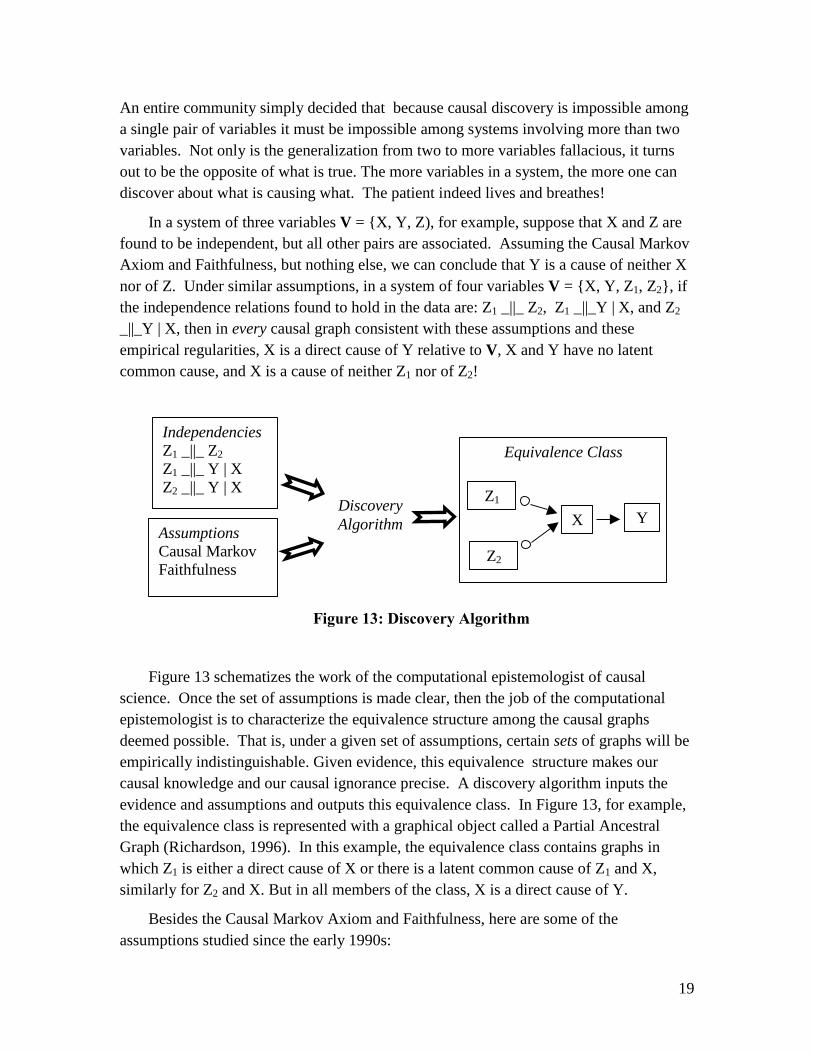
nor of Z. Under similar assumptions, in a system of four variables V = {X, Y, Z1, Z2}, if
the independence relations found to hold in the data are: Z1 _||_ Z2, Z1 _||_Y | X, and Z2
_||_Y | X, then in every causal graph consistent with these assumptions and these
empirical regularities, X is a direct cause of Y relative to V, X and Y have no latent
common cause, and X is a cause of neither Z1 nor of Z2!
Independencies
Z1 _||_ Z2
Z1 _||_ Y | X
Z2 _||_ Y | X
Assumptions
Causal Markov
Faithfulness
Z2
Z1
X Y
Equivalence Class
Discovery
Algorithm
Figure 13: Discovery Algorithm
Figure 13 schematizes the work of the computational epistemologist of causal
science. Once the set of assumptions is made clear, then the job of the computational
epistemologist is to characterize the equivalence structure among the causal graphs
deemed possible. That is, under a given set of assumptions, certain sets of graphs will be
empirically indistinguishable. Given evidence, this equivalence structure makes our
causal knowledge and our causal ignorance precise. A discovery algorithm inputs the
evidence and assumptions and outputs this equivalence class. In Figure 13, for example,
the equivalence class is represented with a graphical object called a Partial Ancestral
Graph (Richardson, 1996). In this example, the equivalence class contains graphs in
which Z1 is either a direct cause of X or there is a latent common cause of Z1 and X,
similarly for Z2 and X. But in all members of the class, X is a direct cause of Y.
Besides the Causal Markov Axiom and Faithfulness, here are some of the
assumptions studied since the early 1990s:
20
D-separation
Causal Sufficiency (no latent common causes)
Feedback
Linearity
Assuming D-separation and Faithfulness, we know how to characterize equivalence over
the following classes of models:
1. Causally sufficient, no feedback, linear.
2. Causally sufficient, no feedback, not linear.
3. Causally sufficient, feedback, linear.
4. Not causally sufficient, no feedback, linear.
5. Not causally sufficient, no feedback, not linear.
When and why one should endorse these various assumptions is another topic, but the
moral should be clear. What one can discover depends on the assumptions made and the
data collected, and the fine grain structure is as rich and complex for the theory of
causation as for any subject I know of.
7. Epilogue
Advancements in causation have not come solely on the theoretician’s side of the
subject. Algorithms have been discovered, implemented, and applied to data sets, and
have produced tangible results. Scheines, Boomsma and Hoijtink (1999), for example,
used these techniques to help decide whether low-level exposure to Lead indeed damages
the cognitive abilities of young children. Ramsey et al. (2000) have applied these
methods to spectra in service of remote classification of rocks (intended for use on Mars),
Bessler and colleagues have applied automatic discovery to farm prices (Bessler and
Akleman (1998), Spirtes and Cooper (1999) have automatically learned causal
relationships from a medical database on pneumonia patients; and, most recently, we
have begun to apply the techniques to learn about genetic regulatory structure (Spirtes,
Glymour and Scheines, 2000a).
The computer has had an incalculably large impact on the theory, and especially the
epistemology of causation. The survey I have given here is no more than the briefest
sketch, however. To learn more, I recommend four books which cover most of the field
and give references to the parts they do not. The 2nd
edition of Spirtes, Glymour and
Scheines (2000) has the most extensive treatment of model equivalence, discovery
algorithms, the axiomatization of causal models, and the faithfulness debate. Pearl
(2000) gives the best comprehensive treatment of the modern representation of the
21
subject, and is the clearest at distinguishing between observation and manipulation and
carrying that distinction all the way through the formalization of the topic. Two edited
collections, one by Glymour and Cooper (1999), and one by McKim and Turner (1997),
pull together a wide array of important writers, many of whom do not agree with each
and are not afraid to say so. These volumes bring to life the debates that still rage about
the subject and make the computational turn in the philosophy of causation accessible.
References
Bessler, D. and Akelman, D. (1998). Farm prices, retail prices and directed graphs:
results for pork and beef. American Journal of Agricultural Economics, 80: 1144-
1149.
Blalock, H. (1961). Causal Inferences in Nonexperimental Research. University of North
Carolina Press, Chapel Hill, NC.
Blalock, H. (1971). Causal Models in the Social Sciences. Aldine-Atherton, Chicago.
Bollen, K. (1989). Structural Equations with Latent Variables. Wiley, New York.
Costner, H. (1971). Theory, deduction and rules of correspondence. Causal Models in the
Social Sciences, Blalock, H. (ed.). Aldine, Chicago.
Fisher, R. (1935, 1951). The Design of Experiments. Oliver and Boyd, Edinburgh.
Glymour, C., Scheines, R., Spirtes, P., and Kelly, K. (1987). Discovering Causal
Structure. Academic Press, San Diego, CA.
Glymour, C., and Cooper, G. (1999). Computation, Causation, and Discovery. AAAI
Press and MIT Press.
Harary, F., and Palmer, E. (1973). Graphical Enumeration. Academic Press, New York.
Hausman, D. (1984). Causal priority. Nous 18, 261-279.
Haavelmo, T. (1943). The statistical implications of a system of simultaneious equations.
Econometrica 11: 1-12. Repreinted in Hendry, D., and Morgan, M. (eds.), The
Foundations of Econometric Analysis, pp. 477-490, Cambridge University Press.
Heise, D. (1975). Causal Analysis. Wiley, New York.
Joreskog, K. (1973). A general method for estimating a linear structural equation.
Structural Equation Models in the Social Sciences, Goldberger, A., and Duncan, O.
(eds.). Seminar Press, New York.
Kiiveri, H. and Speed, T. (1982). Structural analysis of multivariate data: A review.
Sociological Methodology, Leinhardt, S. (ed.). Jossey-Bass, San Francisco.
Kiiveri, H., Speed, T., and Carlin, J. (1984). Recursive causal models. Journal of the
Australian Mathematical Society 36, 30-52.
Lauritzen, S., and Spiegelhalter, D (1988). Local computations with probabilities on
graphical structures and their application to expert systems [with discussion]. Journal
of the royal Statistical Society, Ser. B 50: 157-224.
Lewis, D. (1973). Causation. Journal of Philosophy 70, 556-572.
Mackie, J. (1974). The Cement of the Universe. Oxford University Press, New York.
22
McKim, S., and Turner, S. (1997). Causality in Crisis? Statistical methods and the
Search for Causal Knowledge in the Social Sciences. University of Notre Dame
Press.
Pearl, J. (1988). Probabilistic Reasoning in Intelligent Systems. Morgan and Kaufman,
San Mateo.
Ramsey, J., Gazis, P., Roush, T., Spirtes, P. and Glymour, P. (2000). "Automated
Remote Sensing with Near Infrared Reflectance Spectra: Carbonate Recognition." J.
Knowledge Discovery and Data Mining, under review. (Available at
http://www.phil.cmu.edu/rockspec).
Richardson, T. (1996). Models of Feedback: Interpretation and Discovery. Phd Thesis,
Department of Philsosophy, Carnegie Mellon University, Pittsburgh, PA.
Reichenbach, H. (1956). The Direction of Time. Univ. of California Press, Berkeley, CA.
Rubin, D. (1974). Estimating causal effects of treatments in randomized and
nonrandomized studies. Journal of Educational Psychology 66, 688-701.
Salmon, W. (1980). Probabilistic causality. Pacific Philosophical Quarterly 61, 50-74.
Scheines, R. (1987). Causality in the Social Sciences, Doctoral Dissertation, Dept. of
History and Philosophy of Science, University of Pittsburgh, Pittsburgh, PA.
Scheines, R., Boomsma, A., and Hoijtink, H. (1999). Bayesian Estimation and Testing of
Structural Equation Models. Psychometrika 64: 37-52.
Simon, H. (1953). Causal ordering and identifiability. Studies in Econometric Methods.
Hood and Koopmans (eds). 49-74.Wiley, NY.
Simon, H. (1954).Spurious correlation: a causal interpretation. JASA. 49, 467-479.
Spirtes, P., Cooper, G. (1997). An Experiment in Causal Discovery Using a Pneumonia
Database, Proceedings of AI and Statistics 99.
Spirtes, P., Glymour, C., Scheines R., (1993). Causation, Prediction and Search,
Springer-Verlag.
Spirtes, P., Glymour, C., Scheines R., (2000a). Causation, Prediction and Search, 2nd
Edition, MIT Press, Cambridge, MA.
Spirtes, P., Glymour, C., and Scheines, R. (2000b) Constructing Bayesian Network
Models of Gene Expression Networks from Microarray Data, Proceedings of the
Atlantic Symposium on Computational Biology, Genome Information Systems &
Technology.
Suppes, P. (1970). A Probabilistic Theory of Causality. North-Holland, Amsterdam.
Wermuth, N. and Lauritzen, S. (1983). Graphical and recursive models for contingency
tables. Biometrika 72, 537-552.
Whittaker, J. (1990). Graphical Models in Applied Multivariate Statistics. Wiley, New
York.
Wright, S. (1934). The method of path coefficients. Ann. Math. Stat. 5, 161-215.


