
Computational Economics
Prof. Dr. Maik Wolters
Friedrich-Schiller-University Jena
Overview
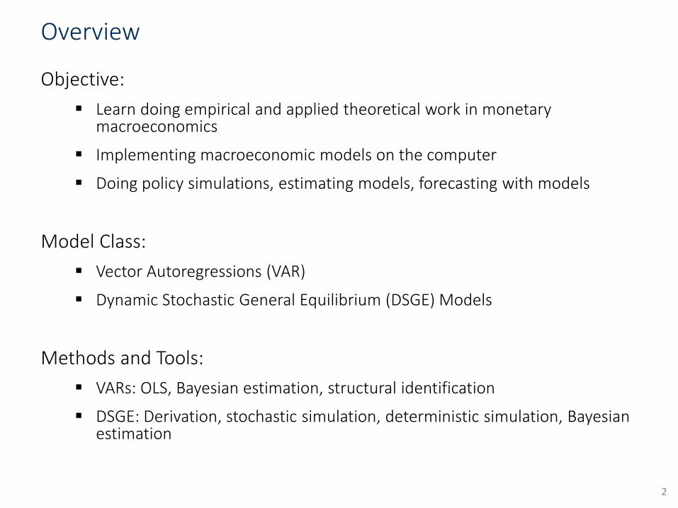
Objective:
Learn doing empirical and applied theoretical work in monetarymacroeconomics
Implementing macroeconomic models on the computer
Doing policy simulations, estimating models, forecasting with models
Model Class:
Vector Autoregressions (VAR)
Dynamic Stochastic General Equilibrium (DSGE) Models
Methods and Tools:
VARs: OLS, Bayesian estimation, structural identification
DSGE: Derivation, stochastic simulation, deterministic simulation, Bayesianestimation
2

Lecturers
Lectures:
Prof. Dr. Maik Wolters, [email protected]
Exercise sessions / Research Project
Lars Other, Office 4.162, [email protected]
Josefine Quast, Office 4.148, [email protected]
Office Hours
By appointment (send an Email)
3

Outline
Part 1: Vector Autoregressions
Part 2: The baseline New Keynesian model – Derivation and stochastic simulations
Part 3: Medium-scale DSGE models – Stochastic simulations
Part 4: Deterministic simulations – Fiscal policy applications
Part 5: Estimation of DSGE models, Forecasting
4
Literature
Macroeconomic Theory:
Walsh, Carl (2010). Monetary Theory and Policy, The MIT Press, Third Edition.
Galí, Jordi (2015). Monetary Policy, Inflation, and the Business Cycle: An Introduction to the New Keynesian Framework and Its Applications, Princeton Press, Second Edition.
Romer, David, (2012). Advanced Macroeconomics, McGraw-Hill, Fourth Edition.
Wickens, Michael (2011). Macroeconomic Theory. A Dynamic General Equilibrium Approach, Princeton University Press, Second Edition.
Heijdra, Ben j. (2017). Foundations of Modern Macroeconomics, Oxford University Press, Third Edition.
Methodology:
Canova, F. (2007). Methods for Applied Macroeconomic Research, Princeton University Press.
DeJong, David N., and Chentan Dave (2011). Structural Macroeconometrics, Princeton University Press, Second Edition.
Lütkepohl, H. (2007). New Introduction to Multiple Time Series Analysis, Springer.
Kilian, L. and H. Lütkepohl (2017). Structural Vector Autoregressive Analysis, Cambridge University Press, http://www-personal.umich.edu/~lkilian/book.html
Dynare User Guide, Dynare Manual.
Academic papers:
Will be announced during the course.
5
6
Part 1
Vector Autoregressions
Data in monetary macroeconomics
Time series of aggregate data
Examples: GDP, CPI inflation, short- and long-term interest rates, exchange rates, …
Frequency: typically quarterly and sometimes monthly
Data availability: only data for few recent decades available
Many structural breaks (different policy regimes, structural change in the economy, etc.)
Typical time series: 80-120 observations in quarterly frequency
7

8
0
2
4
6
8
10
12
14
16
18
1954 1959 1964 1969 1974 1979 1984 1989 1994 1999 2004 2009 2014
3
4
5
6
7
8
9
10
11
1954 1959 1964 1969 1974 1979 1984 1989 1994 1999 2004 2009 2014
-4
-2
0
2
4
6
8
10
1954 1959 1964 1969 1974 1979 1984 1989 1994 1999 2004 2009 2014
-2
0
2
4
6
8
10
12
14
1954 1959 1964 1969 1974 1979 1984 1989 1994 1999 2004 2009 2014
Real GDP growth (year-on-year) Unemployment Rate
CPI Inflation (year-on-year) Fed Funds Rate
Core Macro Time Series (US Data)

Trends and persistence
Some time series show trends and keep growing: GDP, CPI, …
9
2000
4000
6000
8000
10000
12000
14000
16000
18000
1954 1959 1964 1969 1974 1979 1984 1989 1994 1999 2004 2009 2014
20
70
120
170
220
270
Real GDP (level) CPI (level)
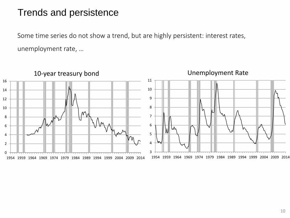
Trends and persistence
Some time series do not show a trend, but are highly persistent: interest rates,
unemployment rate, …
10
3
4
5
6
7
8
9
10
11
1954 1959 1964 1969 1974 1979 1984 1989 1994 1999 2004 2009 2014
Unemployment Rate
0
2
4
6
8
10
12
14
16
1954 1959 1964 1969 1974 1979 1984 1989 1994 1999 2004 2009 2014
10-year treasury bond
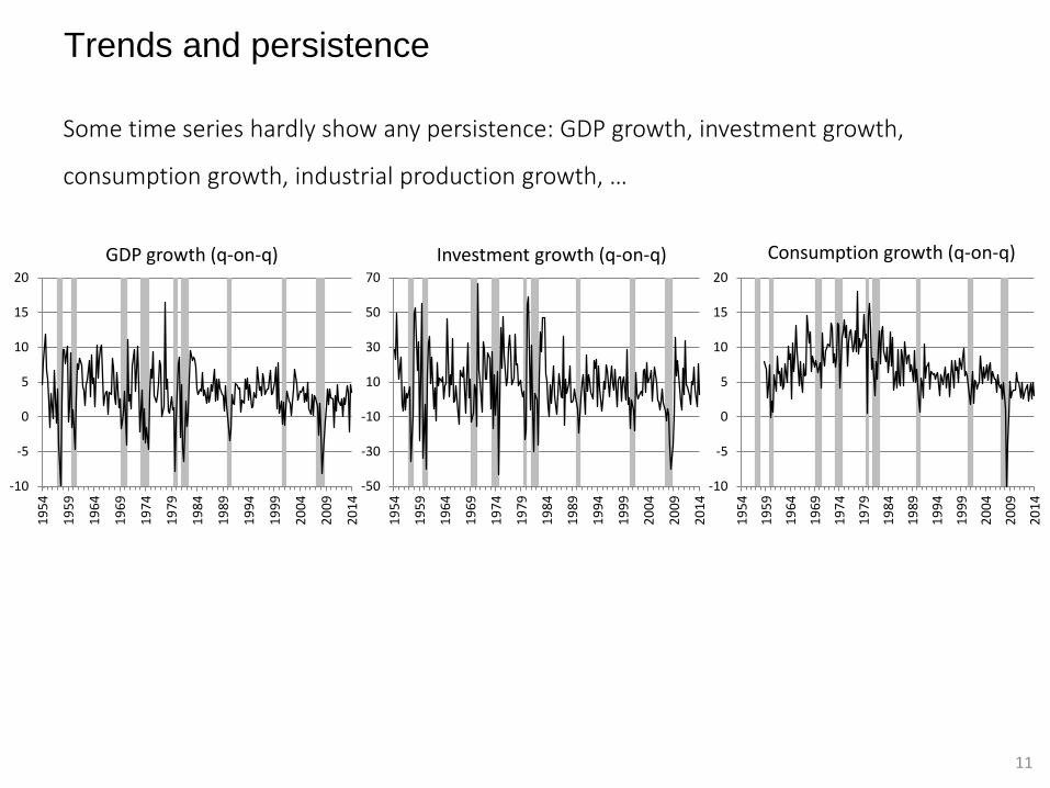
Trends and persistence
Some time series hardly show any persistence: GDP growth, investment growth,
consumption growth, industrial production growth, …
11
-10
-5
0
5
10
15
20
19
54
19
59
19
64
19
69
19
74
19
79
19
84
19
89
19
94
19
99
20
04
20
09
20
14
-50
-30
-10
10
30
50
70
19
54
19
59
19
64
19
69
19
74
19
79
19
84
19
89
19
94
19
99
20
04
20
09
20
14
-10
-5
0
5
10
15
20
19
54
19
59
19
64
19
69
19
74
19
79
19
84
19
89
19
94
19
99
20
04
20
09
20
14
GDP growth (q-on-q) Investment growth (q-on-q) Consumption growth (q-on-q)

Collinearity and dynamic correlation
Macroeconomic datasets are characterized by collinearity
GDP, consumption, investment, industrial production, …
Inflation, interest rates, …
Dynamic interaction of macroeconomic variables
Phillips curve: unemployment rate and inflation
IS-curve: real interest rate and output
Taylor rule: output gap, inflation and interest rate
We do not study univariate time series models (AR, ARMA, ARIMA, ARCH,
GARCH, …), but focus on multivariate models (VAR)
12

Data transformation
Seasonal adjustment
13
Source: Leamer, 2009, Chapter 2
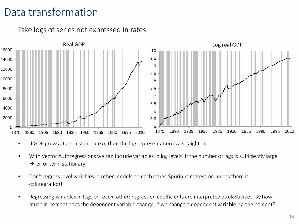
Data transformation
Take logs of series not expressed in rates
• If GDP grows at a constant rate g, then the log representation is a straight line
• With Vector Autoregressions we can include variables in log levels. If the number of lags is sufficiently large
error term stationary
• Don‘t regress level variables in other models on each other. Spurious regression unless there is
cointegration!
• Regressing variables in logs on each other: regression coefficients are interpreted as elasticities. By how
much in percent does the dependent variable change, if we change a dependent variable by one percent?
14
5
5,5
6
6,5
7
7,5
8
8,5
9
9,5
10
1875 1890 1905 1920 1935 1950 1965 1980 1995 20100
2000
4000
6000
8000
10000
12000
14000
16000
1875 1890 1905 1920 1935 1950 1965 1980 1995 2010
Real GDP Log real GDP
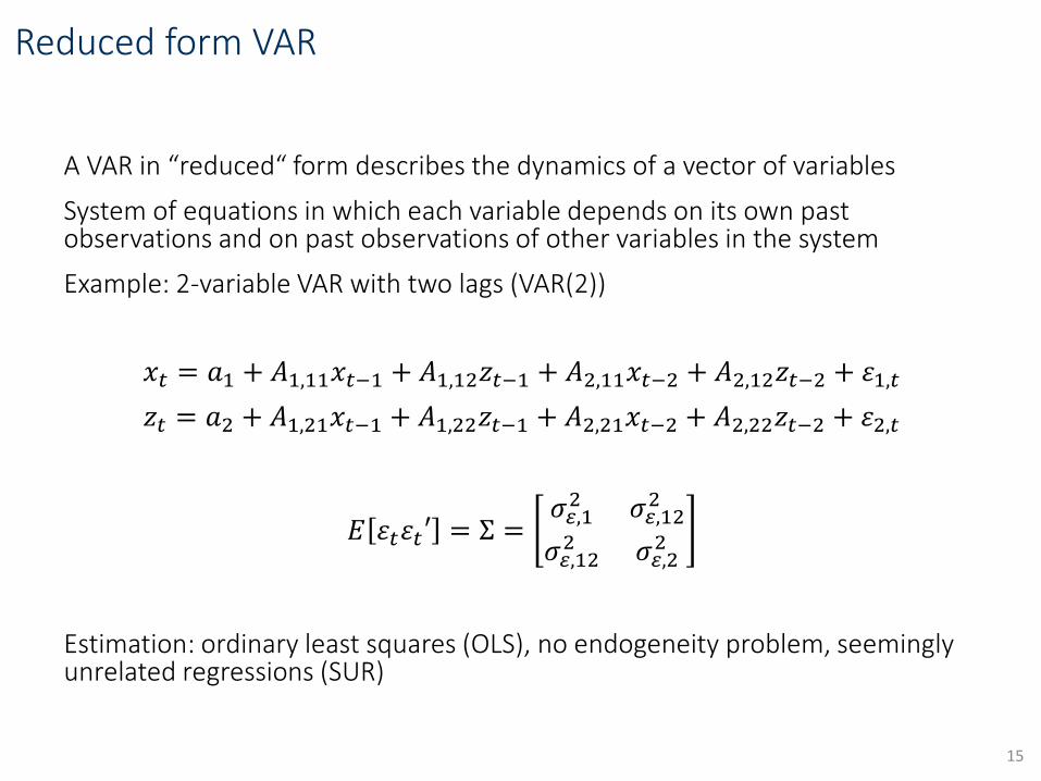
Reduced form VAR
A VAR in “reduced“ form describes the dynamics of a vector of variables
System of equations in which each variable depends on its own pastobservations and on past observations of other variables in the system
Example: 2-variable VAR with two lags (VAR(2))
𝑥𝑡 = 𝑎1 + 𝐴1,11𝑥𝑡−1 + 𝐴1,12𝑧𝑡−1 + 𝐴2,11𝑥𝑡−2 + 𝐴2,12𝑧𝑡−2 + 𝜀1,𝑡
𝑧𝑡 = 𝑎2 + 𝐴1,21𝑥𝑡−1 + 𝐴1,22𝑧𝑡−1 + 𝐴2,21𝑥𝑡−2 + 𝐴2,22𝑧𝑡−2 + 𝜀2,𝑡
𝐸 𝜀𝑡𝜀𝑡′ = Σ =𝜎𝜀,12 𝜎𝜀,12
2
𝜎𝜀,122 𝜎𝜀,2
2
Estimation: ordinary least squares (OLS), no endogeneity problem, seeminglyunrelated regressions (SUR)
15
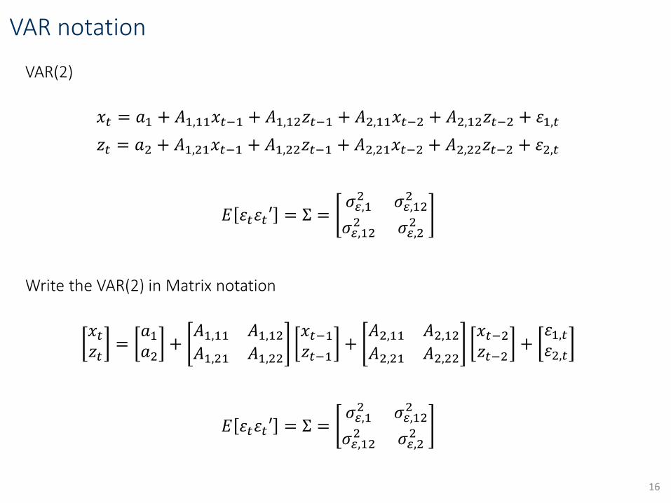
VAR notation
VAR(2)
𝑥𝑡 = 𝑎1 + 𝐴1,11𝑥𝑡−1 + 𝐴1,12𝑧𝑡−1 + 𝐴2,11𝑥𝑡−2 + 𝐴2,12𝑧𝑡−2 + 𝜀1,𝑡
𝑧𝑡 = 𝑎2 + 𝐴1,21𝑥𝑡−1 + 𝐴1,22𝑧𝑡−1 + 𝐴2,21𝑥𝑡−2 + 𝐴2,22𝑧𝑡−2 + 𝜀2,𝑡
𝐸 𝜀𝑡𝜀𝑡′ = Σ =𝜎𝜀,12 𝜎𝜀,12
2
𝜎𝜀,122 𝜎𝜀,2
2
Write the VAR(2) in Matrix notation
𝑥𝑡𝑧𝑡
=𝑎1𝑎2
+𝐴1,11 𝐴1,12
𝐴1,21 𝐴1,22
𝑥𝑡−1𝑧𝑡−1
+𝐴2,11 𝐴2,12
𝐴2,21 𝐴2,22
𝑥𝑡−2𝑧𝑡−2
+𝜀1,𝑡𝜀2,𝑡
𝐸 𝜀𝑡𝜀𝑡′ = Σ =𝜎𝜀,12 𝜎𝜀,12
2
𝜎𝜀,122 𝜎𝜀,2
2
16

VAR notation
VAR(2) in Matrix notation
𝑥𝑡𝑧𝑡
=𝑎1𝑎2
+𝐴1,11 𝐴1,12
𝐴1,21 𝐴1,22
𝑥𝑡−1𝑧𝑡−1
+𝐴2,11 𝐴2,12
𝐴2,21 𝐴2,22
𝑥𝑡−2𝑧𝑡−2
+𝜀1,𝑡𝜀2,𝑡
𝐸 𝜀𝑡𝜀𝑡′ = Σ =𝜎𝜀,12 𝜎𝜀,12
2
𝜎𝜀,122 𝜎𝜀,2
2
Define: Yt =𝑥𝑡𝑧𝑡
VAR(p) in Matrix notation:
𝑌𝑡 = 𝐴(1)𝑌𝑡−1 + 𝐴(2)𝑌𝑡−1 +⋯+ 𝐴 𝑝 𝑌𝑡−𝑝 + 𝜀𝑡
Short notation with lag operator:
𝑌𝑡 = 𝐴 𝐿 𝑌𝑡−1 + 𝜀𝑡, 𝐸 𝜀𝑡𝜀𝑡′ = Σ
𝑌𝑡 can include of course more than 2 variables
17
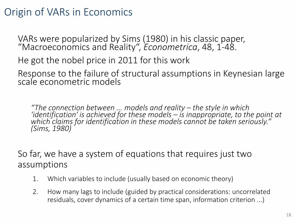
Origin of VARs in Economics
VARs were popularized by Sims (1980) in his classic paper, “Macroeconomics and Reality“, Econometrica, 48, 1-48.
He got the nobel price in 2011 for this work
Response to the failure of structural assumptions in Keynesian large scale econometric models
“The connection between ... models and reality – the style in which‘identification‘ is achieved for these models – is inappropriate, to the point at which claims for identification in these models cannot be taken seriously.“ (Sims, 1980)
So far, we have a system of equations that requires just twoassumptions
1. Which variables to include (usually based on economic theory)
2. How many lags to include (guided by practical considerations: uncorrelatedresiduals, cover dynamics of a certain time span, information criterion ...)
18
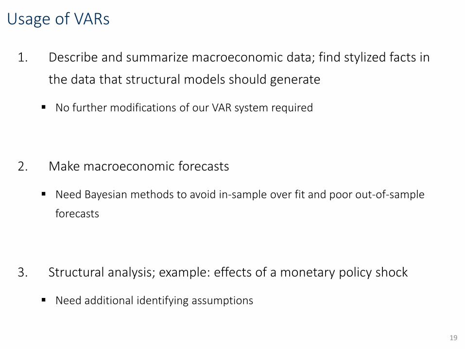
Usage of VARs
1. Describe and summarize macroeconomic data; find stylized facts in
the data that structural models should generate
No further modifications of our VAR system required
2. Make macroeconomic forecasts
Need Bayesian methods to avoid in-sample over fit and poor out-of-sample
forecasts
3. Structural analysis; example: effects of a monetary policy shock
Need additional identifying assumptions
19
1. Desriptive analysis with VARs
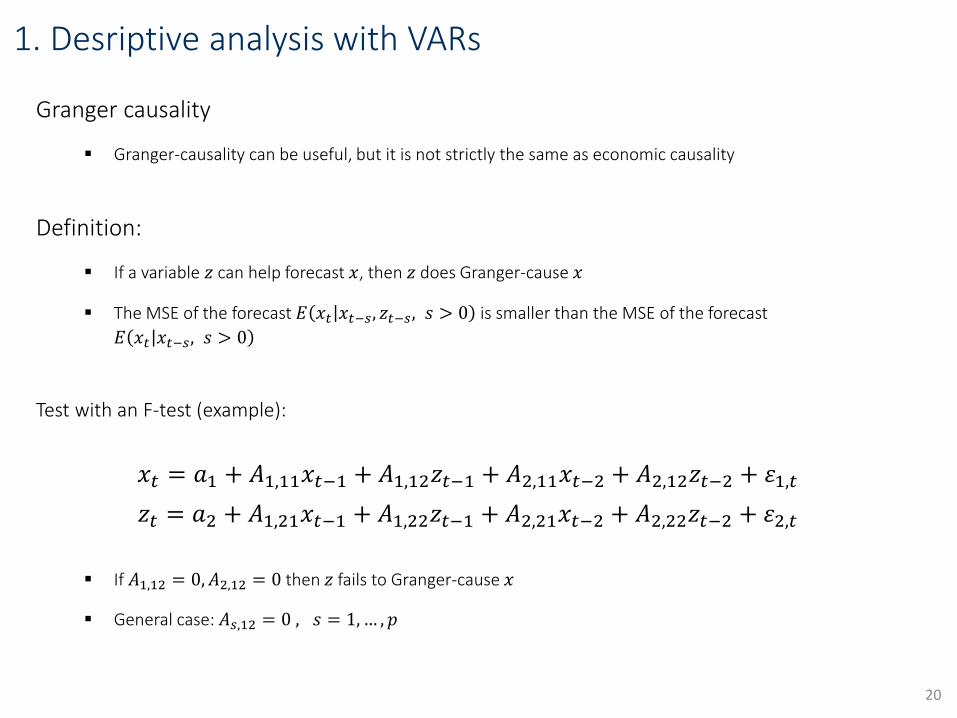
Granger causality
Granger-causality can be useful, but it is not strictly the same as economic causality
Definition:
If a variable 𝑧 can help forecast 𝑥, then 𝑧 does Granger-cause 𝑥
The MSE of the forecast 𝐸 𝑥𝑡 𝑥𝑡−𝑠, 𝑧𝑡−𝑠, 𝑠 > 0 is smaller than the MSE of the forecast
𝐸 𝑥𝑡 𝑥𝑡−𝑠, 𝑠 > 0
Test with an F-test (example):
𝑥𝑡 = 𝑎1 + 𝐴1,11𝑥𝑡−1 + 𝐴1,12𝑧𝑡−1 + 𝐴2,11𝑥𝑡−2 + 𝐴2,12𝑧𝑡−2 + 𝜀1,𝑡
𝑧𝑡 = 𝑎2 + 𝐴1,21𝑥𝑡−1 + 𝐴1,22𝑧𝑡−1 + 𝐴2,21𝑥𝑡−2 + 𝐴2,22𝑧𝑡−2 + 𝜀2,𝑡
If 𝐴1,12 = 0, 𝐴2,12 = 0 then 𝑧 fails to Granger-cause 𝑥
General case: 𝐴𝑠,12 = 0 , 𝑠 = 1,… , 𝑝
20

Granger causality: example with a bivariate VAR
RBC models with nominal neutrality imply that money has no effect on the real variables
Classical dichotomy (real and nominal variables can be analyzedseparately)
We can use a VAR to check whether money in fact does not Granger-cause real variables
Sims (1972) finds that output does not Granger-cause money, but thatmoney Granger causes output
His interpretation was that money supply is exogenous (set by the Fed) and thus isnot influenced by output
On the other hand money has real effects (rejection of the classical dichotomy)
Here, a combination of two Granger causality tests has been used to make an economic interpretation
21

Granger causality: example with a 3-variable VAR
Stock and Watson (2001) use a VAR with inflation, unemployment and the federal funds rate
Table 1 shows p-values of F-tests
VAR can be roughly be interpreted as
Phillips Curve
IS equation (however, inflation not significant)
Taylor Rule
22

2. Forecasting with VARs
Univariate case
Autoregression: AR(p)
𝑥𝑡 = 𝛼 + 𝑎1𝑥𝑡−1 + 𝑎2𝑥𝑡−2 +⋯+ 𝑎𝑝𝑥𝑡−𝑝 + 𝜀𝑡
Forecast is simply obtained by iterating forward
One-step forecast: 𝐸𝑡𝑥𝑡+1 = 𝛼 + 𝑎1𝑥𝑡 + 𝑎2𝑥𝑡−1 +⋯+ 𝑎𝑝𝑥𝑡−𝑝+1 + 𝐸𝑡𝜀𝑡+1
Two-step forecast: 𝐸𝑡𝑥𝑡+2 = 𝛼 + 𝑎1𝐸𝑡𝑥𝑡+1 + 𝑎2𝑥𝑡 +⋯+ 𝑎𝑝𝑥𝑡−𝑝+2 + 𝐸𝑡𝜀𝑡+2
…
h-step in general: 𝐸𝑡𝑥𝑡+ℎ = 𝛼 + 𝑎1𝐸𝑡𝑥𝑡+ℎ−1 +⋯+ 𝑎𝑝𝐸𝑡𝑥𝑡−𝑝+ℎ + 𝐸𝑡𝜀𝑡+ℎ=0
Multivariate model
Consider the following model: 𝑥𝑡 = 𝛼 + 𝑎1𝑥𝑡−1 + 𝑏1𝑧𝑡−1 + 𝜀𝑡
One-step forecast: 𝐸𝑡𝑥𝑡+1= 𝛼 + 𝑎1𝑥𝑡 + 𝑏1𝑧𝑡
Two-step forecast: 𝐸𝑡𝑥𝑡+2 = 𝛼 + 𝑎1𝐸𝑡𝑥𝑡+1 + 𝑏1𝐸𝑡𝑧𝑡+1
VAR(p) model:
Joint forecasting model for all variables that can simply be iterated forward:
𝐸𝑡𝑥𝑡+ℎ = 𝑎1 + 𝐴1,11𝐸𝑡𝑥𝑡+ℎ−1 + 𝐴1,12𝐸𝑡𝑧𝑡+ℎ−1 + 𝐴2,11𝐸𝑡𝑥𝑡+ℎ−2 + 𝐴2,12𝐸𝑡𝑧𝑡+ℎ−2
𝐸𝑡𝑧𝑡+ℎ = 𝑎2 + 𝐴1,21𝐸𝑡𝑥𝑡+ℎ−1 + 𝐴1,22𝐸𝑡𝑧𝑡+ℎ−1 + 𝐴2,21𝐸𝑡𝑥𝑡+ℎ−2 + 𝐴2,22𝐸𝑡𝑧𝑡+ℎ−223
What to use here?

Forecasting with VARs: Example
1. Decide on variables to include in the VAR
2. Decide on number of lags
3. Estimate with OLS
4. Iterate forward to get forecasts
24Source: Stock and Watson (2001)
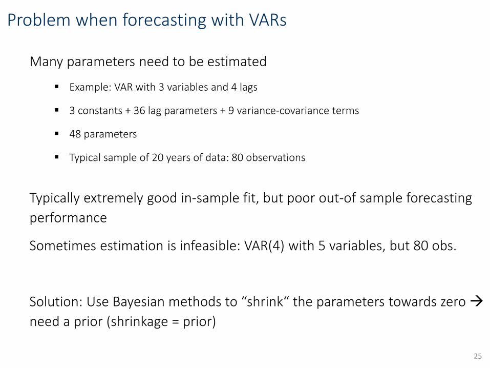
Problem when forecasting with VARs
Many parameters need to be estimated
Example: VAR with 3 variables and 4 lags
3 constants + 36 lag parameters + 9 variance-covariance terms
48 parameters
Typical sample of 20 years of data: 80 observations
Typically extremely good in-sample fit, but poor out-of sample forecasting
performance
Sometimes estimation is infeasible: VAR(4) with 5 variables, but 80 obs.
Solution: Use Bayesian methods to “shrink“ the parameters towards zero
need a prior (shrinkage = prior)
25

The Bayesian approach
Frequentist approach:
Inference by means of hypothesis testing, confidence intervals
Probability viewed as long-run frequency
Unknown „true“ parameters are constant
Bayesian approach:
Inference by means of posterior distributions
Probability viewed as subjective belief
Unknown parameters are treated as random variables with a probability distribution
For forecasting the Bayesian approach can also simply be viewed as a
pragmatic tool to increase forecasting accuracy
26
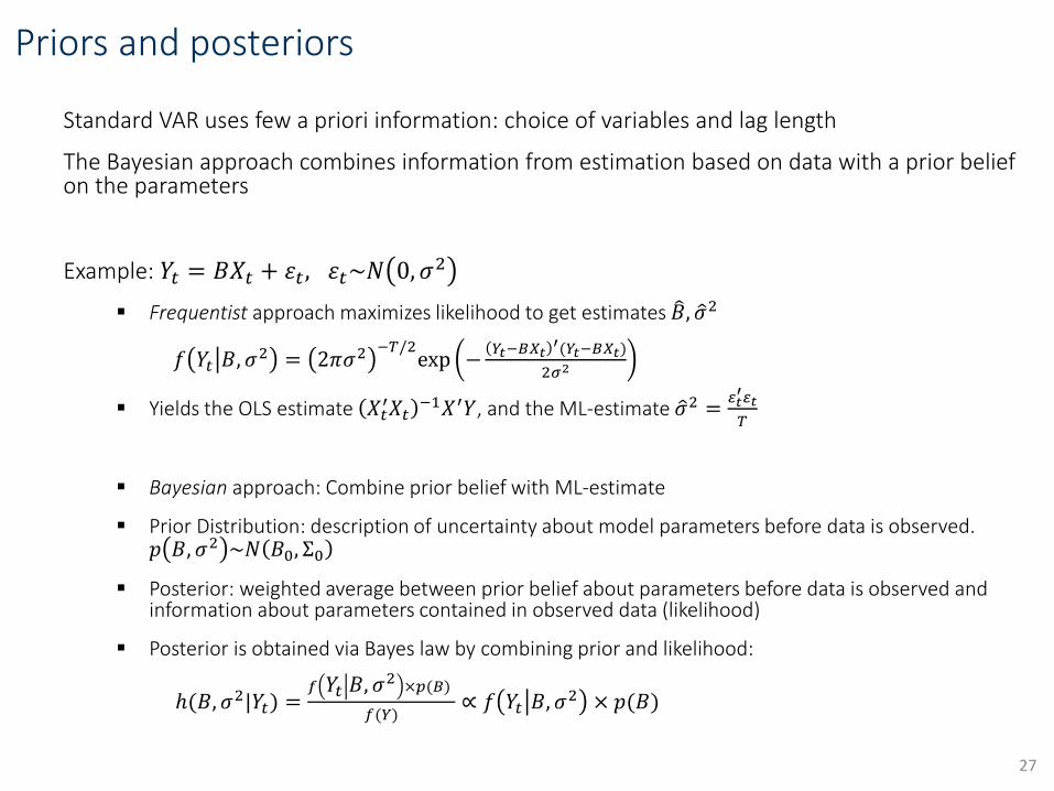
Priors and posteriors
Standard VAR uses few a priori information: choice of variables and lag length
The Bayesian approach combines information from estimation based on data with a prior belief on the parameters
Example: 𝑌𝑡 = 𝐵𝑋𝑡 + 𝜀𝑡, 𝜀𝑡~𝑁 0, 𝜎2
Frequentist approach maximizes likelihood to get estimates 𝐵, 𝜎2
𝑓 𝑌𝑡 𝐵, 𝜎2 = 2𝜋𝜎2 −𝑇/2
exp −𝑌𝑡−𝐵𝑋𝑡
′(𝑌𝑡−𝐵𝑋𝑡)
2𝜎2
Yields the OLS estimate 𝑋𝑡′𝑋𝑡
−1𝑋′𝑌, and the ML-estimate 𝜎2 =𝜀𝑡′𝜀𝑡
𝑇
Bayesian approach: Combine prior belief with ML-estimate
Prior Distribution: description of uncertainty about model parameters before data is observed. 𝑝 𝐵, 𝜎2 ~𝑁 𝐵0, Σ0
Posterior: weighted average between prior belief about parameters before data is observed andinformation about parameters contained in observed data (likelihood)
Posterior is obtained via Bayes law by combining prior and likelihood:
ℎ(𝐵, 𝜎2|𝑌𝑡) =𝑓 𝑌𝑡 𝐵, 𝜎
2×𝑝(𝐵)
𝑓(𝑌)∝ 𝑓 𝑌𝑡 𝐵, 𝜎2 × 𝑝(𝐵)
27
Bayesian VARs
Typical Bayesian analysis involves:
1. Formulation of probability model for the data (here: VAR)
2. Specification of prior distribution for unknown model parameters
3. Construction of likelihood from observed data
4. Combination of prior distribution and likelihood to obtain posterior distribution
of model parameters
5. Bayesian Inference
28

Minnesota prior
Prior developed to achieve a good forecasting model
Achieve a parsimonous model by shrinking parameters towards zero
Developed by Litterman and Sims at the University of Minnesota and the Federal Reserve Bank of
Minneapolis
VAR: 𝑥𝑡 = 𝑎1 + 𝐴1,11𝑥𝑡−1 + 𝐴1,12𝑧𝑡−1 + 𝐴2,11𝑥𝑡−2 + 𝐴2,12𝑧𝑡−2 + 𝜀1,𝑡
𝑧𝑡 = 𝑎2 + 𝐴1,21𝑥𝑡−1 + 𝐴1,22𝑧𝑡−1 + 𝐴2,21𝑥𝑡−2 + 𝐴2,22𝑧𝑡−2 + 𝜀2,𝑡
𝐸 𝜀𝑡𝜀𝑡′ = Σ
Need a prior for 𝐴1,11, … , 𝐴2,22 and Σ
Minnesota prior simplifies by replacing Σ with an estimate Σ need only priors for 𝐴1,11, … , 𝐴2,22
Minnesota prior assumes that most time series can be described as a random walk (with drift) process: 𝑥𝑡 = 𝛼 + 𝑥𝑡−1 + 𝜀𝑡
Coefficient of 1 on first lag of own variable
Coefficient of 0 on all other lags of own variable
Coefficient of 0 on other variables
29
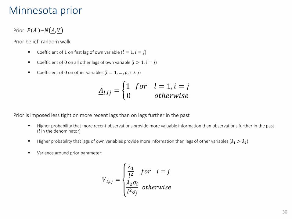
Minnesota prior
Prior: 𝑃 𝐴 ~𝑁 𝐴, 𝑉
Prior belief: random walk
Coefficient of 1 on first lag of own variable (𝑙 = 1, 𝑖 = 𝑗)
Coefficient of 0 on all other lags of own variable (𝑙 > 1, 𝑖 = 𝑗)
Coefficient of 0 on other variables (𝑙 = 1,… , 𝑝, 𝑖 ≠ 𝑗)
𝐴𝑙,𝑖𝑗 = 1 𝑓𝑜𝑟 𝑙 = 1, 𝑖 = 𝑗0 𝑜𝑡ℎ𝑒𝑟𝑤𝑖𝑠𝑒
Prior is imposed less tight on more recent lags than on lags further in the past
Higher probability that more recent observations provide more valuable information than observations further in the past(𝑙 in the denominator)
Higher probability that lags of own variables provide more information than lags of other variables (𝜆1 > 𝜆2)
Variance around prior parameter:
𝑉𝑙,𝑖𝑗 =
𝜆1𝑙2
𝑓𝑜𝑟 𝑖 = 𝑗
𝜆2𝜎𝑖𝑙2𝜎𝑗
𝑜𝑡ℎ𝑒𝑟𝑤𝑖𝑠𝑒
30

Illustration: Minnesota prior
31
Source: Canova (2007)
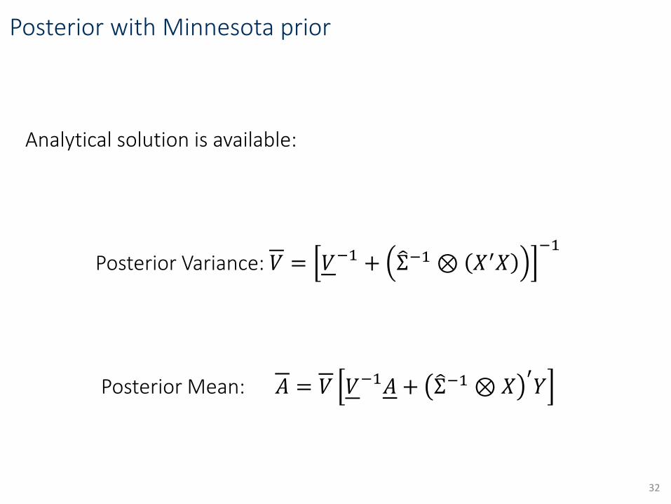
Posterior with Minnesota prior
Analytical solution is available:
Posterior Variance: 𝑉 = 𝑉−1 + Σ−1 ⊗ 𝑋′𝑋−1
Posterior Mean: 𝐴 = 𝑉 𝑉−1𝐴 + Σ−1 ⊗𝑋′𝑌
32

Example: BVAR with Minnesota prior
• Forecasting German macroeconomic variables (Pirschel and Wolters, 2017)
• Variables: GDP, CPI, short-term interest rate, unemployment rate
Bayesian VAR: 4 lags, Normal-Wishart Minnesota prior
Unrestricted VAR: number of lags chosen with Bayesian Information Criterion
Evaluation sample: 1994Q4-2013Q4
33
horizon BVAR: RMSFE VAR: RMSFE
1 (GDP) 3.29 3.72
4 (GDP) 3.44 3.95
8 (GDP) 3.51 3.55
1 (CPI) 1.33 1.43
4 (CPI) 1.29 1.52
8 (CPI) 1.35 1.65

3. Structural VARs
So far the reduced form VAR was restricted to dynamic interactions betweenvariables
This assumption is implausible for structural analysis. Variables depend on each otheralso in period 𝑡 and not only in 𝑡 − 1, 𝑡 − 2,…
Structural form 2-variable VAR with 2 lags: SVAR(2)
𝐹11𝑥𝑡 + 𝐹12𝑧𝑡 = 𝑏1 + 𝐵1,11𝑥𝑡−1 + 𝐵1,12𝑧𝑡−1 + 𝐵2,11𝑥𝑡−2 + 𝐵2,12𝑧𝑡−2 + 𝑢1,𝑡
𝐹21𝑥𝑡 + 𝐹22𝑧𝑡 = 𝑏2 + 𝐵1,21𝑥𝑡−1 + 𝐵1,22𝑧𝑡−1 + 𝐵2,21𝑥𝑡−2 + 𝐵2,22𝑧𝑡−2 + 𝑢2,𝑡
𝐸 𝑢𝑡𝑢𝑡′ = D =𝜎𝑢,12 𝜎𝑢,12
2
𝜎𝑢,122 𝜎𝑢,2
2
This could be a structural model derived from theory. Traditional Cowles commissionmodels have this structure
Structural parameters 𝐹, 𝐵, 𝐷 are different from the reduced form parameters 𝐴, Σ. In particular the structural shocks 𝑢𝑖,𝑡 are different from the reduced form shocks 𝜀𝑖,𝑡.
34
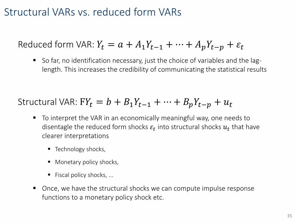
Structural VARs vs. reduced form VARs
Reduced form VAR: 𝑌𝑡 = 𝑎 + 𝐴1𝑌𝑡−1 +⋯+ 𝐴𝑝𝑌𝑡−𝑝 + 𝜀𝑡
So far, no identification necessary, just the choice of variables and the lag-length. This increases the credibility of communicating the statistical results
Structural VAR: F𝑌𝑡 = 𝑏 + 𝐵1𝑌𝑡−1 +⋯+ 𝐵𝑝𝑌𝑡−𝑝 + 𝑢𝑡
To interpret the VAR in an economically meaningful way, one needs todisentagle the reduced form shocks 𝜀𝑡 into structural shocks 𝑢𝑡 that haveclearer interpretations
Technology shocks,
Monetary policy shocks,
Fiscal policy shocks, ...
Once, we have the structural shocks we can compute impulse responsefunctions to a monetary policy shock etc.
35
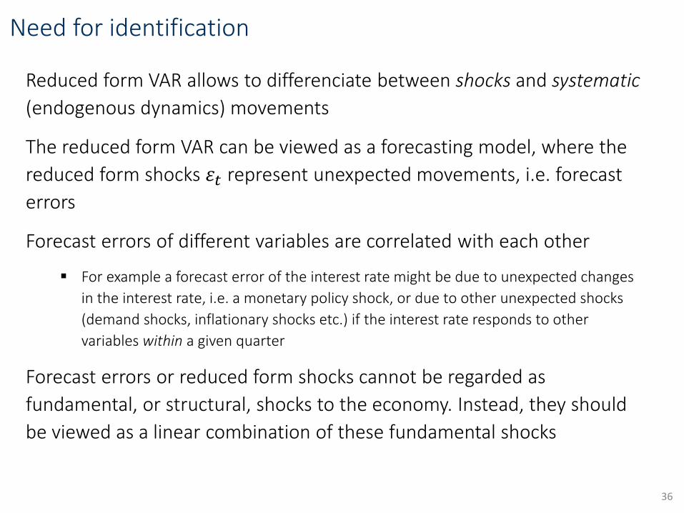
Need for identification
Reduced form VAR allows to differenciate between shocks and systematic
(endogenous dynamics) movements
The reduced form VAR can be viewed as a forecasting model, where the
reduced form shocks 𝜀𝑡 represent unexpected movements, i.e. forecast
errors
Forecast errors of different variables are correlated with each other
For example a forecast error of the interest rate might be due to unexpected changes
in the interest rate, i.e. a monetary policy shock, or due to other unexpected shocks
(demand shocks, inflationary shocks etc.) if the interest rate responds to other
variables within a given quarter
Forecast errors or reduced form shocks cannot be regarded as
fundamental, or structural, shocks to the economy. Instead, they should
be viewed as a linear combination of these fundamental shocks
36
Mapping the structural form into the reduced form
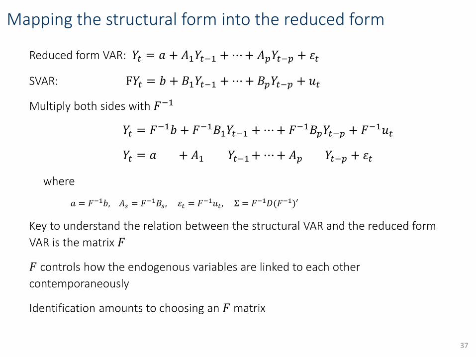
Reduced form VAR: 𝑌𝑡 = 𝑎 + 𝐴1𝑌𝑡−1 +⋯+ 𝐴𝑝𝑌𝑡−𝑝 + 𝜀𝑡
SVAR: F𝑌𝑡 = 𝑏 + 𝐵1𝑌𝑡−1 +⋯+ 𝐵𝑝𝑌𝑡−𝑝 + 𝑢𝑡
Multiply both sides with 𝐹−1
𝑌𝑡 = 𝐹−1𝑏 + 𝐹−1𝐵1𝑌𝑡−1 +⋯+ 𝐹−1𝐵𝑝𝑌𝑡−𝑝 + 𝐹−1𝑢𝑡
𝑌𝑡 = 𝑎 + 𝐴1 𝑌𝑡−1+⋯+ 𝐴𝑝 𝑌𝑡−𝑝 + 𝜀𝑡
where
𝑎 = 𝐹−1𝑏, 𝐴𝑠 = 𝐹−1𝐵𝑠, 𝜀𝑡 = 𝐹−1𝑢𝑡, Σ = 𝐹−1𝐷(𝐹−1)′
Key to understand the relation between the structural VAR and the reduced form
VAR is the matrix 𝐹
𝐹 controls how the endogenous variables are linked to each other
contemporaneously
Identification amounts to choosing an 𝐹 matrix
37
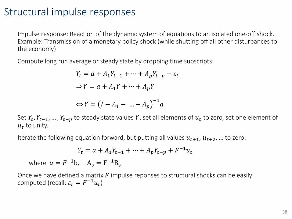
Structural impulse responses
Impulse response: Reaction of the dynamic system of equations to an isolated one-off shock. Example: Transmission of a monetary policy shock (while shutting off all other disturbances tothe economy)
Compute long run average or steady state by dropping time subscripts:
𝑌𝑡 = 𝑎 + 𝐴1𝑌𝑡−1 +⋯+ 𝐴𝑝𝑌𝑡−𝑝 + 𝜀𝑡
𝑌 = 𝑎 + 𝐴1𝑌 +⋯+ 𝐴𝑝𝑌
𝑌 = 𝐼 − 𝐴1 − …− 𝐴𝑝−1𝑎
Set 𝑌𝑡 , 𝑌𝑡−1, … , 𝑌𝑡−𝑝 to steady state values 𝑌, set all elements of 𝑢𝑡 to zero, set one element of𝑢𝑡 to unity.
Iterate the following equation forward, but putting all values 𝑢𝑡+1, 𝑢𝑡+2, … to zero:
𝑌𝑡 = 𝑎 + 𝐴1𝑌𝑡−1 +⋯+ 𝐴𝑝𝑌𝑡−𝑝 + 𝐹−1𝑢𝑡
where 𝑎 = 𝐹−1b, As = F−1Bs
Once we have defined a matrix 𝐹 impulse reponses to structural shocks can be easilycomputed (recall: 𝜀𝑡 = 𝐹−1𝑢𝑡)
38

Structural identification
Structural VAR
F𝑌𝑡 = 𝑏 + 𝐵1𝑌𝑡−1 +⋯+ 𝐵𝑝𝑌𝑡−𝑝 + 𝑢𝑡, 𝐶𝑜𝑣 𝑢𝑡 = 𝐷
Includes 𝑝 + 1 𝑛2 parameters in 𝐹, 𝐵1, … , 𝐵𝑝 , 𝑛 parameters in 𝑏 and 𝑛 + 1 𝑛/2 in 𝐷 (it is
symmetric)
Reduced form VAR
𝑌𝑡 = 𝑎 + 𝐴1𝑌𝑡−1 +⋯+ 𝐴𝑝𝑌𝑡−𝑝 + 𝜀𝑡 , 𝐶𝑜𝑣 𝜀𝑡 = Σ
Includes 𝑝𝑛2 parameters in 𝐴1, … , 𝐴𝑝 , 𝑛 parameters in 𝑎 and 𝑛 + 1 𝑛/2 in Σ
The SVAR includes more parameters than estimated in the reduced form VAR.
We have to impose restrictions on the SVAR to have a clear one-to-one
mapping between the parameters of the two VARs
We have to impose 𝑛2 restrictions on the structural parameters
𝐹, 𝐵1, … , 𝐵𝑝, 𝑏, 𝐷 to identifiy all of them
39

Recursive identification (Sims, 1980)
Impose restrictions on the contemporaneous response of the different endogenous
variables to the different structural shocks
Example: interest rate reacts contemporaneously to monetary policy shocks and to
inflationary shocks. Inflation reacts contemporaneously to inflationary shocks, but only with
a lag to monetary policy shocks
Implement this identification scheme via assuming that 𝐹 is lower triangular and 𝐷 being
diagonal (diagonal elements are the variances of shocks):
First variable can react to lags and the first shock
Second variable can react to lags and the first two shocks
Third variable can react to lags and the first three shocks...
Need to be careful how to order the variables (guided by economic theory)
Number of restrictions on 𝐹: 𝑛(𝑛 + 1)/2
Number of restrictions on 𝐷: 𝑛(𝑛 − 1)/2
Overall number of restrictions: 𝑛²
40
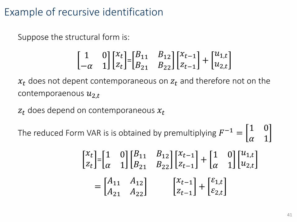
Example of recursive identification
Suppose the structural form is:
1 0−𝛼 1
𝑥𝑡𝑧𝑡
=𝐵11 𝐵12
𝐵21 𝐵22
𝑥𝑡−1𝑧𝑡−1
+𝑢1,𝑡𝑢2,𝑡
𝑥𝑡 does not depent contemporaneous on 𝑧𝑡 and therefore not on the
contemporaenous 𝑢2,𝑡
𝑧𝑡 does depend on contemporaneous 𝑥𝑡
The reduced Form VAR is is obtained by premultiplying 𝐹−1 =1 0𝛼 1
𝑥𝑡𝑧𝑡
=1 0𝛼 1
𝐵11 𝐵12
𝐵21 𝐵22
𝑥𝑡−1𝑧𝑡−1
+1 0𝛼 1
𝑢1,𝑡𝑢2,𝑡
=𝐴11 𝐴12
𝐴21 𝐴22
𝑥𝑡−1𝑧𝑡−1
+𝜀1,𝑡𝜀2,𝑡
41

Example of recursive identification
The reduced Form VAR is is obtained by premultiplying 𝐹−1 =1 0𝛼 1
𝑥𝑡𝑧𝑡
=1 0𝛼 1
𝐵11 𝐵12
𝐵21 𝐵22
𝑥𝑡−1𝑧𝑡−1
+1 0𝛼 1
𝑢1,𝑡𝑢2,𝑡
=𝐴11 𝐴12
𝐴21 𝐴22
𝑥𝑡−1𝑧𝑡−1
+𝜀1,𝑡𝜀2,𝑡
𝜀1,𝑡 = 𝑢1,𝑡
𝜀2,𝑡 = 𝛼𝑢1,𝑡 + 𝑢2,𝑡, so the second reduced form shock is a linear combination of thefirst two structural shocks
The covariance matrix is:
𝐶𝑜𝑣𝜀1,𝑡𝜀2,𝑡
= 𝐹−1𝐷 𝐹−1 ′ =𝜎𝑢,12 𝛼𝜎𝑢,1
2
𝛼𝜎𝑢,12 𝛼2𝜎𝑢,1
2 + 𝜎22 𝐶𝑜𝑣
𝑢1,𝑡𝑢2,𝑡
=𝜎𝑢,12 0
0 𝜎22
42

Bring SVAR into a form with identity covariance matrix
To recover the SVAR from the estimated reduced form VAR the Cholesky
decomposition is used
Rewrite the SVAR: instead of lower triangular with unity elements on the
diagonal of 𝐹 and the diagonal of 𝐷 representing the variances of the
structural shocks, we can write 𝐹 in general lower triangular form
Example: premultiply the structural form by1/𝜎𝑢,1 0
0 1/𝜎𝑢,2
1/𝜎𝑢,1 0
−𝛼/𝜎𝑢,1 1/𝜎𝑢,2
𝑥𝑡𝑧𝑡
=𝐵11/𝜎𝑢,1 𝐵12/𝜎𝑢,1𝐵21/𝜎𝑢,2 𝐵22/𝜎𝑢,2
𝑥𝑡−1𝑧𝑡−1
+𝑢1,𝑡/𝜎𝑢,1𝑢2,𝑡/𝜎𝑢,1
This structual form has a triangular 𝐹 matrix and a covariance matrix equal to
an identity matrix 𝐼
43

Cholesky decomposition
We estimate Σ = 𝐹−1𝐼( 𝐹−1)′ and want to find 𝐹
We know that 𝐹 is lower triangular
Let Σ be a 𝑛𝑥𝑛 symmetric positive definite matrix. The Cholesky decomposition
gives the unique lower triangular matrix 𝑃 such that Σ = 𝑃′𝑃
Step 1: From Σ = 𝐹−1𝐼( 𝐹−1)′ (recall 𝐷 = 𝐼 is assumed) the Cholesky
decomposition recovers 𝐹−1. Invert to get 𝐹, which is triangular
Step 2: Compute the structural parameters:
𝑏 = 𝐹 a, 𝐵𝑠 = 𝐹 𝐴𝑠
44

Application: Monetary policy transmission
Study the transmission of a monetary policy shock on key
macroeconomic aggregates
• Main reference: Christiano, L. J., M. Eichenbaum and C. L. Evans (1999).
“Monetary policy shocks: What have we learned and to what end?“
Handbook of Macroeconomics.
Stylized facts
Interest rates initially rise
Aggregate price level initially responds very little. Price level decreasesafter 1-2 years
Aggregate output initially falls with a zero long-run effect
45

Set up a monetary SVAR
Structural VAR with Cholesky identification to study the
transmission of a structural monetary policy shock to the economy
GDP, consumption, investment
GDP deflator, commodity price index
Fed Funds Rate, 10-year Rate, non-borrowed reserves, total
reserves
46
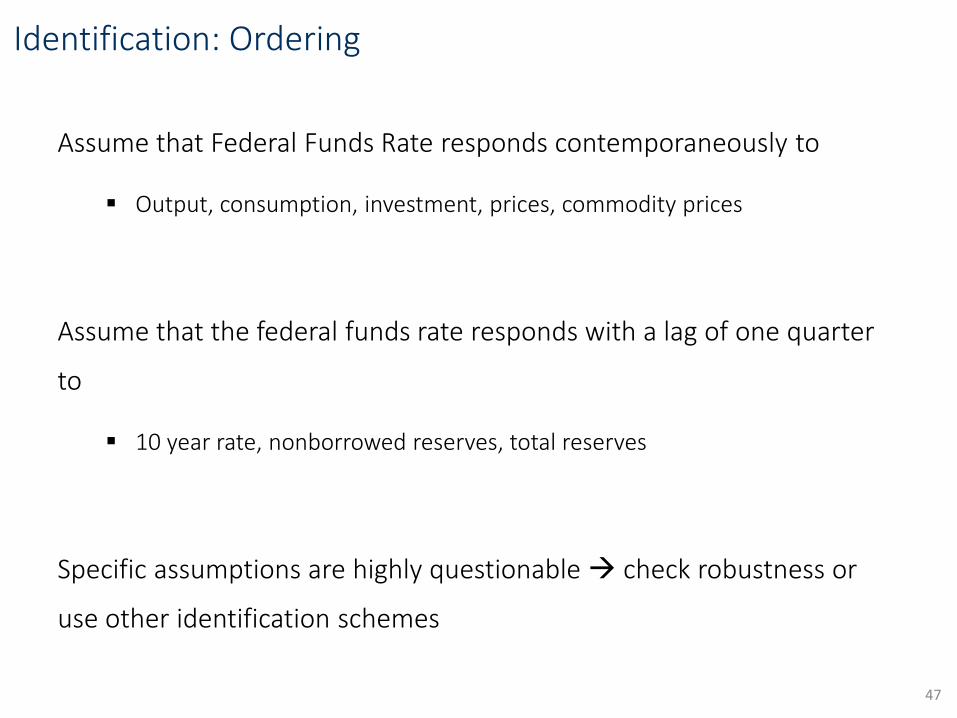
Identification: Ordering
Assume that Federal Funds Rate responds contemporaneously to
Output, consumption, investment, prices, commodity prices
Assume that the federal funds rate responds with a lag of one quarter
to
10 year rate, nonborrowed reserves, total reserves
Specific assumptions are highly questionable check robustness or
use other identification schemes
47

48

Monetary policy transmission
49
Summary
VARs are one of the most important analysis tools in monetary
macroeconomics
Account for collinearity and dynamic correlation between variables
Need a minimum number of assumptions let the data speak
Three application areas
1. Desriptive analysis: need to choose number of variables and lags
2. Forecasting: need to shrink parameters towards zero BVAR
3. Structural analysis: need additional identification assumptions.
VAR methodology is restricted to study the transmission of one
time (temporary) suprise changes in policy. To study permanent
changes in policy regimes we need structural models.
50
ReferencesOverview VARs:
Stock, James H. and Mark W. Watson (2001). “Vector Autoregressions”, Journal of Economic Perspectives, 15(4): 101-115.
Structural Identification
Söderlind, P. (2005). “Lecture Notes in Empirical Macroeconomics”, available online on Paul Söderlind’swebsite.
Kilian, L. (2013). “Structural Vectorautoregressions“, in Handbook of Research Methods and Applications, Chapter 22.
Lütkepohl, H., and M. Krätzig (2004). “Applied Time Series Econometrics“, Cambridge University Press, Chapters 3 and 4.
Enders, W. (2004). “Applied Econometric Time Series“, John Wiley & Sons, Ch. 5.
Bayesian VARs
Koop, G., and D. Korobilis (2010). “Bayesian Multivariate Time Series Methods for Empirical Macroeconomics”, available on Gary Koop’s website
Canova, F. (2007). “Methods for Applied Macroeconomic Research“, Princeton University Press, Chapter 10.
Forecasting with Bayesian VARs
Karlsson, S. (2013). “Forecasting with Bayesian Vectorautoregressions“, Handbook of EconomicForecasting, Vol. 2, Chapter 15.
Bayesian VAR: Gibbs sampler (simulating the posterior distribution)
Blake, A., and H. Mumtaz (2012). “Applied Bayesian econometrics for central bankers“, Technical Handbook No. 4, Center for Central Banking Studies, Bank of England.
51


