


Final Report Conceptual Model for the Refined Seymour Aquifer Groundwater Availability Model: Haskell, Knox, and Baylor Counties Prepared by:
Toya L. Jones, P.G. John E. Ewing, P.E. Tingting Yan John F. Pickens, Ph.D., P.E., P.G. Bridget R. Scanlon, Ph.D., P.G. Jeff Olyphant Andrew Chastain-Howley, P.G., MCSM Prepared for:
Texas Water Development Board February 2012


Conceptual Model for the Refined Seymour Aquifer Groundwater Availability Model: Haskell, Knox, and Baylor Counties
Final Report Conceptual Model for the Refined Seymour Aquifer Groundwater Availability Model: Haskell, Knox, and Baylor Counties
Prepared by:
Toya L. Jones, P.G. John E. Ewing, P.E. Tingting Yan John F. Pickens, Ph.D., P.E. P.G. INTERA Incorporated
Bridget R. Scanlon, Ph.D., P.G. Jeff Olyphant Bureau of Economic Geology University of Texas at Austin
Andrew Chastain-Howley, P.G., MCSM Water Prospecting Resource Consultants, LLC
Prepared for:
Texas Water Development Board
February 2012

ii
This page is intentionally blank.

Conceptual Model for the Refined Seymour Aquifer Groundwater Availability Model: Haskell, Knox, and Baylor Counties
iv
This page intentionally left blank.

Conceptual Model for the Refined Seymour Aquifer Groundwater Availability Model: Haskell, Knox, and Baylor Counties
v
Table of Contents
1.0 Introduction ......................................................................................................................... 1-1
2.0 Study Area .......................................................................................................................... 2-1 2.1 Physiography and Climate ...................................................................................... 2-11 2.2 Geology .................................................................................................................. 2-27 2.3 Brief Land Use History of Baylor, Knox, and Haskell Counties ........................... 2-39
3.0 Previous Investigations ....................................................................................................... 3-1
4.0 Hydrogeologic Setting ........................................................................................................ 4-1 4.1 Hydrostratigraphy ..................................................................................................... 4-5 4.2 Structure ................................................................................................................... 4-7 4.3 Water Levels and Regional Groundwater Flow ..................................................... 4-15
4.3.1 Historical Water-Level Fluctuations in the Seymour Aquifer ................... 4-16 4.3.2 Regional Groundwater Flow ...................................................................... 4-20 4.3.3 Steady-State Conditions ............................................................................. 4-21 4.3.4 Water-Level Elevations for Transient Model Calibration .......................... 4-21 4.3.5 Cross-Formational Flow ............................................................................. 4-23 4.3.6 Transient Water Levels .............................................................................. 4-26
4.4 Recharge ................................................................................................................. 4-63 4.4.1 Methods Used to Estimate Recharge ........................................................ 4-66
4.4.1.1 Chloride Mass Balance Method ................................................. 4-66 4.4.1.2 Water-Table Fluctuation Method ............................................... 4-68
4.4.2 Results and Discussion ............................................................................. 4-68 4.4.2.1 Chloride Mass Balance Method ................................................. 4-69 4.4.2.2 Water-Table Fluctuation Method ............................................... 4-72
4.4.3 Summary and Recommendations ............................................................. 4-74 4.5 Rivers, Streams, Springs, and Lakes ...................................................................... 4-89
4.5.1 Rivers and Streams ..................................................................................... 4-89 4.5.2 Springs ........................................................................................................ 4-91 4.5.3 Lakes and Reservoirs .................................................................................. 4-92
4.6 Hydraulic Properties ............................................................................................. 4-105 4.6.1 Data Sources ............................................................................................... 4-105 4.6.2 Calculation of Hydraulic Conductivity from Specific Capacity ................. 4-105 4.6.3 Analysis of the Hydraulic Property Data .................................................... 4-106 4.6.4 Variogram Analysis of Hydraulic Conductivity ......................................... 4-107 4.6.5 Spatial Distribution of Hydraulic Conductivity .......................................... 4-108 4.6.6 Vertical Hydraulic Conductivity ................................................................. 4-108 4.6.7 Storativity .................................................................................................... 4-109
4.7 Aquifer Discharge ................................................................................................ 4-117 4.7.1 Natural Discharge ..................................................................................... 4-117 4.7.2 Aquifer Discharge through Pumping ....................................................... 4-119
4.7.2.1 Methodology ............................................................................. 4-119 4.7.2.2 Pumping Plots and Tables ......................................................... 4-122
4.8 Water Quality in the Seymour Aquifer ................................................................ 4-135
Groundwater Availability Model for the Refined Seymour Aquifer: Haskell, Knox, and Baylor Counties
Table of Contents, continued
vi
4.8.1 Previous Studies ....................................................................................... 4-135 4.8.2 Data Sources and Methods of Analysis .................................................... 4-135 4.8.3 Results ...................................................................................................... 4-136
4.8.3.1 Drinking Water Quality ............................................................. 4-136 4.8.3.2 Irrigation Water Quality ............................................................ 4-138
5.0 Conceptual Model of Groundwater Flow for the refined Seymour Aquifer Groundwater Availability Model .............................................................................................................. 5-1
6.0 References .......................................................................................................................... 6-1
Appendix A Results of Investigation of Likely Completion of UNKNOWN wells located in the Seymour Aquifer
Appendix B Draft Conceptual Model Report Comments and Responses

Groundwater Availability Model for the Refined Seymour Aquifer: Haskell, Knox, and Baylor Counties
vii
List of Figures
Figure 1.0.1 Locations of major aquifers in Texas (TWDB, 2006a). ...................................... 1-4 Figure 1.0.2 Locations of minor aquifers in Texas (TWDB, 2006b). ...................................... 1-5 Figure 2.0.1 Location of study area and model boundary for the refined Seymour
Aquifer groundwater availability model. ............................................................. 2-2 Figure 2.0.2 Location of study area showing county boundaries, cities, and major
roadways (TWDB, 2006c; TWDB, 2006d). ........................................................ 2-3 Figure 2.0.3 Location of study area showing lakes and rivers (TWDB, 2007a;
Alexander and others, 1999). ............................................................................... 2-4 Figure 2.0.4 Areal extent of major aquifers in the study area (TWDB, 2006a). ...................... 2-5 Figure 2.0.5 Locations of Regional Water Planning Areas in the study area
(TWDB, 2008a). .................................................................................................. 2-6 Figure 2.0.6 Location of the Groundwater Conservation District in the study area
from the October 2008 Groundwater Conservation District map (TWDB, 2009a). .................................................................................................. 2-7
Figure 2.0.7 Location of the Groundwater Management Area in the study area (TWDB, 2007b). .................................................................................................. 2-8
Figure 2.0.8 Location of River Authorities in the study area (TWDB, 1999). ........................ 2-9 Figure 2.0.9 Major river basins in the study area (TWDB, 2008b). ...................................... 2-10 Figure 2.1.1 Physiographic province in the study area (University of Texas at
Austin, Bureau of Economic Geology, 1996). ................................................... 2-14 Figure 2.1.2 Ecological region in the study area (Texas Parks and Wildlife, 2009). ............. 2-15 Figure 2.1.3 Topographic map of the study (United States Geological Survey,
2006). ................................................................................................................. 2-16 Figure 2.1.4 Climate classification in the study area (Larkin and Bomar, 1983). ................. 2-17 Figure 2.1.5 Average annual air temperature in the study area (Texas A&M
University, 2002). .............................................................................................. 2-18 Figure 2.1.6 Average minimum, mid-range, and maximum monthly temperatures at
two locations in the study area (National Climatic Data Center, 2001). ........... 2-19 Figure 2.1.7 Location of precipitation gages in the study area (National Climatic
Data Center, 2001). ............................................................................................ 2-20 Figure 2.1.8 Annual precipitation time series at two locations in the study area
(National Climatic Data Center, 2001). ............................................................. 2-21 Figure 2.1.9 Average annual precipitation over the study area (Oregon State
University, 2002). .............................................................................................. 2-22 Figure 2.1.10 Average annual net pan evaporation over the study area (TWDB,
2009b). ............................................................................................................... 2-23 Figure 2.1.11 Average monthly lake surface evaporation for one-degree quadrangle
408 in the study area (TWDB, 2009b). .............................................................. 2-24 Figure 2.1.12 Potential evapotranspiration in the study area (Borrelli and others,
1998). ................................................................................................................. 2-25 Figure 2.2.1 Major structural features in the study area (Price, 1979). .................................. 2-31 Figure 2.2.2 Surface geology of the study area (United States Geological Survey-
Texas Water Science Center and the Texas Natural Resources Information System, 2004). ............................................................................... 2-32

Groundwater Availability Model for the Refined Seymour Aquifer: Haskell, Knox, and Baylor Counties
List of Figures, continued
viii
Figure 2.2.3 Schematic of generalized stratigraphy across the study area. ............................ 2-33 Figure 2.2.4 Location of older and younger Seymour Formation deposits (from
R.W. Harden and Associates, 1978). ................................................................. 2-34 Figure 2.2.5 A-A', B-B', C-C', and D-D' cross-sections from R.W. Harden and
Associates (1978) showing the Seymour Formation and Clear Fork Group in Haskell and Knox counties. ................................................................ 2-35
Figure 2.2.6 E-E', F-F', and G-G' cross-sections from R.W. Harden and Associates (1978) showing the Seymour Formation and Clear Fork Group in Haskell and Knox counties. ............................................................................... 2-36
Figure 2.2.7 Geologic cross-section through the Seymour Formation in Baylor County (from Preston, 1978). ............................................................................ 2-37
Figure 3.0.1 Location of extent and active area for the Seymour Aquifer groundwater availability model (Ewing and others, 2004) and the refined groundwater availability model for the Haskell-Knox-Baylor pod of the Seymour Aquifer. ............................................................................... 3-3
Figure 4.0.1 Outline of the Seymour Aquifer as defined by the TWDB and of the water-bearing portion of the Seymour Formation as defined by R.W. Harden and Associates (1978). ............................................................................ 4-4
Figure 4.2.1 Data sources for the Seymour Aquifer structure. ............................................... 4-10 Figure 4.2.2 Structure map of the top of the Seymour Aquifer. ............................................. 4-11 Figure 4.2.3 Structure map of the base of the Seymour Aquifer. ........................................... 4-12 Figure 4.2.4 Isopach map of the Seymour Aquifer. ............................................................... 4-13 Figure 4.2.5 Structure map of the top of the Clear Fork Group. ............................................ 4-14 Figure 4.3.1 Water-level measurement locations for the Seymour Aquifer and
Permian-age formations in the study area. ......................................................... 4-37 Figure 4.3.2 Temporal distribution of water-level measurements in the Seymour
Aquifer in the study area. ................................................................................... 4-38 Figure 4.3.3 Water-level rises reported in the Seymour Formation in western
Haskell County by Bandy (1934) (from R.W. Harden and Associates, 1978). ................................................................................................................. 4-39
Figure 4.3.4 Groundwater flow directions in the Seymour Aquifer in Haskell and southern Knox counties (from R.W. Harden and Associates, 1978). ................ 4-40
Figure 4.3.5 Elevations of springs flowing from the Seymour Aquifer under steady-state conditions................................................................................................... 4-41
Figure 4.3.6 Estimated steady-state water-level elevation contours for the Permian-age formations in the study area. ....................................................................... 4-42
Figure 4.3.7 Locations of data points used to develop estimated steady-state, 1980, 1990, and 1997 water-level elevation contours for the Permian-age formations. ......................................................................................................... 4-43
Figure 4.3.8 Estimated water-level elevation contours in the Seymour Aquifer in the study area at the start of the transient model calibration period (January 1980). .................................................................................................. 4-44

Groundwater Availability Model for the Refined Seymour Aquifer: Haskell, Knox, and Baylor Counties
List of Figures, continued
ix
Figure 4.3.9 Estimated water-level elevation contours in the Seymour Aquifer in the study area at the middle of the transient model calibration period (January 1990). .................................................................................................. 4-45
Figure 4.3.10 Estimated water-level elevation contours in the Seymour Aquifer in the study area at the end of the transient model calibration period (December 1997). .............................................................................................. 4-46
Figure 4.3.11 Estimated 1980 to 1997 trends in water-level elevations in the Seymour Aquifer in the study area. ................................................................... 4-47
Figure 4.3.12 Estimated water-level elevation contours in the Permian-age formations in the study area at the start of the transient model calibration period (January 1980). ..................................................................... 4-48
Figure 4.3.13 Estimated water-level elevation contours in the Permian-age formations in the study area at the middle of the transient model calibration period (January 1990). ..................................................................... 4-49
Figure 4.3.14 Estimated water-level elevation contours in the Permian-age formations in the study area at the end of the transient model calibration period (December 1997). ................................................................. 4-50
Figure 4.3.15 Comparison of water-level elevations in the Seymour Aquifer and underlying Clear Fork Group in the study area. ................................................ 4-51
Figure 4.3.16 Locations of Seymour Aquifer wells in the study area with transient water-level data. ................................................................................................. 4-52
Figure 4.3.17 Hydrographs for the five Seymour Aquifer wells in Baylor County with long-term transient water-level data. ......................................................... 4-53
Figure 4.3.18 Example hydrographs showing fluctuating water-level elevations with time in the Seymour Aquifer in Haskell County. .............................................. 4-54
Figure 4.3.19 Example hydrographs showing increasing and stable water-level elevations with time in the Seymour Aquifer in Haskell County. ..................... 4-55
Figure 4.3.20 Hydrographs for the four Seymour Aquifer wells in Knox County with long-term transient water-level data showing a decreasing trend. ..................... 4-56
Figure 4.3.21 Hydrographs for the five Seymour Aquifer wells in Knox County with long-term transient water-level data showing a decreasing and then increasing trend. ................................................................................................. 4-57
Figure 4.3.22 Hydrographs for the four Seymour Aquifer wells in Knox County with long-term transient water-level data showing an increasing trend. ................... 4-58
Figure 4.3.23 Hydrographs for the three Seymour Aquifer wells in Knox County with long-term transient water-level data showing a stable trend. .................... 4-59
Figure 4.3.24 Hydrographs for the three Seymour Aquifer wells with sufficient data to evaluate long-term seasonal fluctuations in water-level elevations. .............. 4-60
Figure 4.3.25 Hydrographs for the 15 Seymour Aquifer wells in Baylor County with data to evaluate seasonal fluctuations between December 1968 and February 1970. ................................................................................................... 4-61
Figure 4.4.1 Land use based on cultivated areas (modified from United States Geological Survey, 1992) and irrigated agriculture. .......................................... 4-80

Groundwater Availability Model for the Refined Seymour Aquifer: Haskell, Knox, and Baylor Counties
List of Figures, continued
x
Figure 4.4.2 Clay content in surface soil (United States Department of Agriculture, 2007). ................................................................................................................. 4-81
Figure 4.4.3 Annual precipitation for the city of Haskell (National Climatic Data Center, 2008)...................................................................................................... 4-82
Figure 4.4.4 Location of boreholes for the unsaturated zone studies in the Seymour Aquifer. .............................................................................................................. 4-83
Figure 4.4.5 Relationship between (a) water content and sand content and (b) water content and clay content for boreholes in the unsaturated zone studies in the Seymour Aquifer. ..................................................................................... 4-84
Figure 4.4.6 Relationship between matric potential and chloride concentration for boreholes in the unsaturated zone studies in the Seymour Aquifer. .................. 4-85
Figure 4.4.7 Long-term water-level data used to estimate recharge rates for the Seymour Aquifer using the water-table fluctuation method. ............................. 4-86
Figure 4.4.8 Estimated spatial distribution of modern recharge for the Seymour Aquifer. .............................................................................................................. 4-87
Figure 4.5.1 Locations of major river, large creeks, and small creeks in the model area. .................................................................................................................... 4-98
Figure 4.5.2 Hydrograph of yearly average stream flow for the gage on the Brazos River in Baylor County. ..................................................................................... 4-99
Figure 4.5.3 Hydrograph of (a) daily and (b) monthly average stream flow for the gage on the Brazos River in Baylor County during the calibration period (1980 to 1997)....................................................................................... 4-100
Figure 4.5.4 Locations of springs flowing from the Seymour Aquifer in the study area. .................................................................................................................. 4-101
Figure 4.5.5 Hydrographs of discharge for selected springs flowing from the Seymour Aquifer. ............................................................................................. 4-102
Figure 4.5.6 Locations of springs and zones of springs and seeps given in R.W. Harden and Associates (1978). ........................................................................ 4-103
Figure 4.5.7 Locations of reservoirs and playas in the study area. ...................................... 4-104 Figure 4.6.1 Locations and sources of hydraulic property data for the Seymour
Aquifer. ............................................................................................................ 4-111 Figure 4.6.2 Empirical correlation between transmissivity (T) and specific capacity
(Sc) for the Seymour Aquifer. ......................................................................... 4-112 Figure 4.6.3 Histogram of hydraulic conductivity data for the Seymour Aquifer. .............. 4-113 Figure 4.6.4 Experimental variogram of log10 of hydraulic conductivity for the
Seymour Aquifer. ............................................................................................. 4-114 Figure 4.6.5 Kriged map of hydraulic conductivity for the Seymour Aquifer. .................... 4-115 Figure 4.6.6 Location of older and younger deposits within the Seymour Aquifer. ............ 4-116 Figure 4.7.1 Population density for the model area. ............................................................ 4-128 Figure 4.7.2 Total groundwater withdrawals from the Haskell-Knox-Baylor pod of
the Seymour Aquifer by category. ................................................................... 4-129 Figure 4.7.3 Yearly average pumpage from the Haskell-Knox-Baylor pod of the
Seymour Aquifer for 1980 through 1997......................................................... 4-130

Groundwater Availability Model for the Refined Seymour Aquifer: Haskell, Knox, and Baylor Counties
List of Figures, continued
xi
Figure 4.7.4 Groundwater withdrawals from 1980 through 1997 for the portion of the Seymour Aquifer in Baylor County considered by this study. .................. 4-131
Figure 4.7.5 Groundwater withdrawals from 1980 through 1997 for the Seymour Aquifer in Haskell County. .............................................................................. 4-132
Figure 4.7.6 Groundwater withdrawals from 1980 through 1997 for the portion of the Seymour Aquifer in Knox County considered by this study. .................... 4-133
Figure 4.7.7 Groundwater withdrawals from 1980 through 1997 for the portion of the Seymour Aquifer in Stonewall County considered by this study. ............. 4-134
Figure 4.8.1 Nitrate concentrations in the groundwater in the Seymour Aquifer. ............... 4-141 Figure 4.8.2 Time series of nitrate concentrations in the Seymour Aquifer at
selected wells. .................................................................................................. 4-142 Figure 4.8.3 Fluoride concentrations in the Seymour Aquifer. ............................................ 4-143 Figure 4.8.4 Total dissolved solids concentrations in the Seymour Aquifer. ...................... 4-144 Figure 4.8.5 Time series of total dissolved solids concentrations in the Seymour
Aquifer for selected wells. ............................................................................... 4-145 Figure 4.8.6 Chloride concentrations in the Seymour Aquifer. ........................................... 4-146 Figure 4.8.7 Time series of chloride concentration and chloride/sulfate ratio for
selected wells. .................................................................................................. 4-147 Figure 4.8.8 Chloride to sulfate ratios in the Seymour Aquifer. .......................................... 4-148 Figure 4.8.9 Salinity hazard of groundwater in the Seymour Aquifer. ................................ 4-149 Figure 4.8.10 Sodium hazard (sodium adsorption ratio) of groundwater in the
Seymour Aquifer. ............................................................................................. 4-150 Figure 5.0.1 Conceptual groundwater flow model (cross-sectional view) for the
refined groundwater availability model for the Haskell-Knox-Baylor pod of the Seymour Aquifer. ............................................................................... 5-8

Groundwater Availability Model for the Refined Seymour Aquifer: Haskell, Knox, and Baylor Counties
xii
This page is intentionally blank.

Groundwater Availability Model for the Refined Seymour Aquifer: Haskell, Knox, and Baylor Counties
xiii
List of Tables
Table 2.2.1 Rock units in the study area (after United States Geological Survey-Texas Water Science Center and the Texas Natural Resources Information System, 2004). ............................................................................... 2-30
Table 2.3.1 Cumulative enrollment in the Conservation Reserve Program (United States Department of Agriculture, 2009). .......................................................... 2-42
Table 4.1.1 Hydrostratigraphy. ............................................................................................... 4-6 Table 4.2.1 Data sources for the basal elevation of the Seymour Aquifer. ............................ 4-9 Table 4.3.1 Comparison of average 1980, 1990, and 1997 water-level elevations in
the Seymour Aquifer. ......................................................................................... 4-30 Table 4.3.2 Summary of data used to compare water-level elevations in the
Seymour Aquifer and the underlying Clear Fork Group. .................................. 4-32 Table 4.3.3 Summary of transient water-level data for the Seymour Aquifer. ..................... 4-33 Table 4.4.1 Land use based on cultivated areas. ................................................................... 4-77 Table 4.4.2 Summary of development of irrigation pumpage in Haskell and Knox
counties from 1950 to 1956 (after Ogilbee and Osborne, 1962). ...................... 4-77 Table 4.4.3 Summary of recharge rates estimated from unsaturated zone studies in
the Seymour Aquifer. ......................................................................................... 4-78 Table 4.4.4 Average water-level rises reported in Bandy (1934) for the Rochester
and O’Brien areas in Haskell County (after R.W. Harden and Associates, 1978). .............................................................................................. 4-79
Table 4.4.5 Recharge rates estimated using the water-table fluctuation method and long-term water-level data for three Seymour Aquifer wells. ........................... 4-79
Table 4.4.6 Summary of all estimates of recharge rate for the Seymour Aquifer. ............... 4-79 Table 4.5.1 Summary of the February 1970 gain/loss study on the Brazos River in
Baylor County (after Preston, 1978). ................................................................. 4-94 Table 4.5.2 Summary of springs flowing from the Seymour Aquifer in the study
area. .................................................................................................................... 4-95 Table 4.6.1 Summary statistics for hydraulic conductivity data (feet per day) for
the Seymour Aquifer and Clear Fork Formation. ............................................ 4-110 Table 4.6.2 Specific yield values for the Seymour Aquifer from the literature. ................. 4-110 Table 4.7.1 Available data on historical pumpage from the Seymour Aquifer
between 1900 and 1979. .................................................................................. 4-124 Table 4.7.2 Total pumping in acre-feet per year by county for 1980, 1985, 1990,
1995, and 1997. ................................................................................................ 4-126 Table 4.7.3 Irrigation pumping in acre-feet per year by county for 1980, 1985,
1990, 1995, and 1997. ...................................................................................... 4-126 Table 4.7.4 Municipal pumping in acre-feet per year by county for 1980, 1985,
1990, 1995, and 1997. ...................................................................................... 4-126 Table 4.7.5 Rural domestic pumping in acre-feet per year by county for 1980,
1985, 1990, 1995, and 1997. ............................................................................ 4-126 Table 4.7.6 Livestock pumping in acre-feet per year by county for 1980, 1985,
1990, 1995, and 1997. ...................................................................................... 4-127 Table 4.7.7 Mining pumping in acre-feet per year by county for 1980, 1985, 1990,
1995, and 1997. ................................................................................................ 4-127

Groundwater Availability Model for the Refined Seymour Aquifer: Haskell, Knox, and Baylor Counties
List of Tables, continued
xiv
Table 4.8.1 Occurrence and levels of some commonly measured groundwater quality constituents in the Haskell-Knox-Baylor pod of the Seymour Aquifer. ............................................................................................................ 4-140
Table 5.0.1 Summary of conditions in the Seymour Aquifer. ................................................ 5-7
Conceptual Model for the Refined Seymour Aquifer Groundwater Availability Model: Haskell, Knox, and Baylor Counties
1-1
1.0 Introduction
The Texas Water Development Board (TWDB) has identified the major and minor aquifers in
Texas on the basis of regional extent and amount of water produced. The major and minor
aquifers are shown in Figures 1.0.1 and 1.0.2, respectively. General discussion of the major and
minor aquifers is given in Ashworth and Hopkins (1995). Aquifers that supply large quantities
of water over large areas of the state are defined as major aquifers and those that supply
relatively small quantities of water over large areas of the state or supply large quantities of
water over small areas of the state are defined as minor aquifers (Ashworth and Hopkins, 1995).
A groundwater availability model was completed for the entire Seymour Aquifer, a major aquifer
in Texas, in 2004 (Ewing and others, 2004). That modeling effort used a single model to
represent the entire Seymour Aquifer, which consists of isolated "pods" that are not hydraulically
connected. In their discussion of possible future improvements, Ewing and others (2004)
recommended that future modeling of the Seymour Aquifer consider each pod individually using
a refined grid design based on the size of the pod, the hydraulic stresses within the pod, and the
ultimate goals of the model. They suggested that the large pod of the Seymour Aquifer located
in Haskell, southern Knox, and western Baylor counties (pod 7 in their report) was a candidate
for a refined model due to the quantity of pumping occurring in that pod of the aquifer.
Consequently, a refined groundwater availability model was developed for the portion of the
Seymour Aquifer located in Haskell, southern Knox, and western Baylor counties. The TWDB
has recently decided to provide documentation of conceptual models and the resulting numerical
groundwater flow models in two separate reports. This report documents the development of the
conceptual model for the portion of the Seymour Aquifer located in Haskell, southern Knox, and
western Baylor counties. A conceptual model assembles field data collected on the aquifer;
allows the researchers to identify system boundaries and hydrostratigraphic units; and provides
the foundation for building a numerical groundwater flow model (Anderson and Woessner,
1992). It is through this process that a better understanding of the aquifer flow system is
ascertained.

Conceptual Model for the Refined Seymour Aquifer Groundwater Availability Model: Haskell, Knox, and Baylor Counties
1-2
The refined model will provide an improved tool for the Rolling Plains Groundwater
Conservation District, the TWDB, and the Region B and G Regional Water Planning Areas to
perform groundwater management and planning. In the remainder of this report, reference to the
Seymour Aquifer means the Haskell-Knox-Baylor pod of the Seymour Aquifer considered by
this study, unless specifically stated otherwise.
The majority of the water pumped from the Seymour Aquifer is used for irrigation purposes
(Ashworth and Hopkins, 1995) with minor pumpage for livestock, domestic, municipal, and
manufacturing uses. Groundwater in the Seymour Aquifer is predominately fresh with slightly
saline groundwater is some areas.
The modeling approach adopted for the refined model of the Seymour Aquifer is to represent the
aquifer as a single layer and the upper portion of the underlying Permian-age strata as a second
layer having separate hydraulic characteristics. The second layer was included in the model to
capture any cross-formational flow between the Seymour Aquifer to the underlying Permian-age
strata.
The Texas Water Code codified the requirement for generation of a State Water Plan that allows
for the development, management, and conservation of water resources and the preparation and
response to drought, while maintaining sufficient water available for the citizens of Texas
(TWDB, 2002). Senate Bill 1 and subsequent legislation directed the TWDB to coordinate
regional water planning with a process based upon public participation.
Groundwater models provide a tool to estimate groundwater availability for various water use
strategies and to determine the cumulative effects of increased water use and drought. A
groundwater model is a numerical representation of the aquifer system capable of simulating
historical conditions and predicting future aquifer conditions. Inherent to the groundwater model
are a set of equations that are developed and applied to describe the physical processes
considered to be controlling groundwater flow in the aquifer system. Groundwater models are
essential to performing complex analyses and in making informed predictions and related
decisions (Anderson and Woessner, 1992). As a result, development of groundwater availability
models for the major and minor Texas aquifers is integral to the state water planning process.
The purpose of the groundwater availability model program is to provide a tool that can be used

Conceptual Model for the Refined Seymour Aquifer Groundwater Availability Model: Haskell, Knox, and Baylor Counties
1-3
to develop reliable and timely information on groundwater availability for the citizens of Texas
and to ensure adequate supplies or recognize inadequate supplies over a 50-year planning period.
The groundwater availability models also serve as an integral part of the process of determining
managed available groundwater based on desired future conditions, as required by House Bill
1763 passed in 2005 by the 79th Legislature. Managed available groundwater was later re-
defined in Senate Bill 737 passed in 2011 by the 82nd Legislature as modeled available
groundwater. Modeled available groundwater is the amount of water that can be produced on an
average annual basis to achieve a desired future condition as established by the groundwater
conservation districts located within 16 groundwater management areas within Texas.
The modeling protocol standard to the groundwater modeling industry includes: (1) the
development of a conceptual model for groundwater flow in the aquifer, (2) model design,
(3) model calibration, (4) sensitivity analysis, and (5) reporting. The conceptual model is a
conceptual description of the physical processes that govern groundwater flow in the aquifer
system. Available data and reports for the model area were reviewed in development of the
conceptual model. The conceptual model describes the hydrostratigraphy, structure, regional
groundwater flow, transient groundwater conditions, recharge to, natural discharge from,
hydraulic properties, water quality, and discharge via pumping for the aquifer.
Consistent with state water planning policy, the conceptual model for the Haskell-Knox-Baylor
pod of the Seymour Aquifer was developed with the support of stakeholders through stakeholder
forums. The purpose of the conceptual model documented here is to provide a description of the
processes needed for development of a refined numerical groundwater availability model for the
Seymour aquifer. The refined groundwater availability model will then provide a tool for
Regional Water Planning Areas, Groundwater Conservation Districts, River Authorities, state
planners, and other stakeholders for the evaluation of groundwater availability and to support the
development of water management strategies and drought planning. The refined Seymour
Aquifer groundwater availability model falls within two of the sixteen Texas Regional Water
Planning Areas and one Groundwater Conservation District.

Conceptual Model for the Refined Seymour Aquifer Groundwater Availability Model: Haskell, Knox, and Baylor Counties
1-4
0 50 100
Miles
Aquifer
OutcropDowndip
Pecos Valley
OutcropDowndip
OutcropDowndip
Gulf Coast
Hueco-Mesilla Bolson
Ogallala
Seymour
OutcropDowndip
Carrizo-Wilcox
Edwards
Edwards-Trinity (Plateau) Trinity
Gulf Coast
Ogallala
Edwards-Trinity (Plateau)
Pecos Valley
Hueco-Mesilla Bolson
Seymour
Carrizo-Wilcox
Edwards
Trinity
Figure 1.0.1 Locations of major aquifers in Texas (TWDB, 2006a).

Conceptual Model for the Refined Seymour Aquifer Groundwater Availability Model: Haskell, Knox, and Baylor Counties
1-5
MarbleFalls
0 50 100
Miles
Blaine
Woodbine
QueenCity
Blossom
BrazosRiver
Alluvium
Yegua-Jackson
Sparta
Nacatoch
RitaBlanca
Dockum
Edwards-Trinity(High
Plains)
Lipan
Ellenburger-San Saba
Bone Spring-Victorio Peak
Igneous
Rustler
CapitanReef
Complex
Marathon
WestTexasBolson
Hickory
Aquifer
OutcropDowndip
Blaine
Blossom
Bone Spring-Victorio Peak
Brazos River Alluvium
Capitan Reef Complex
Dockum
Edwards-Trinity(High Plains)
Ellenburger-San Saba
Hickory
Igneous
Lipan
Marathon
Marble Falls
Nacatoch
Queen City
Rita Blanca
Rustler
Sparta
West Texas Bolson
Woodbine
Yegua - Jackson
OutcropDowndip
OutcropDowndip
OutcropDowndip
OutcropDowndip
OutcropDowndip
OutcropDowndip
OutcropDowndip
OutcropDowndip
OutcropDowndip
Figure 1.0.2 Locations of minor aquifers in Texas (TWDB, 2006b).

Conceptual Model for the Refined Seymour Aquifer Groundwater Availability Model: Haskell, Knox, and Baylor Counties
1-6
This page is intentionally blank.

Conceptual Model for the Refined Seymour Aquifer Groundwater Availability Model: Haskell, Knox, and Baylor Counties
2-1
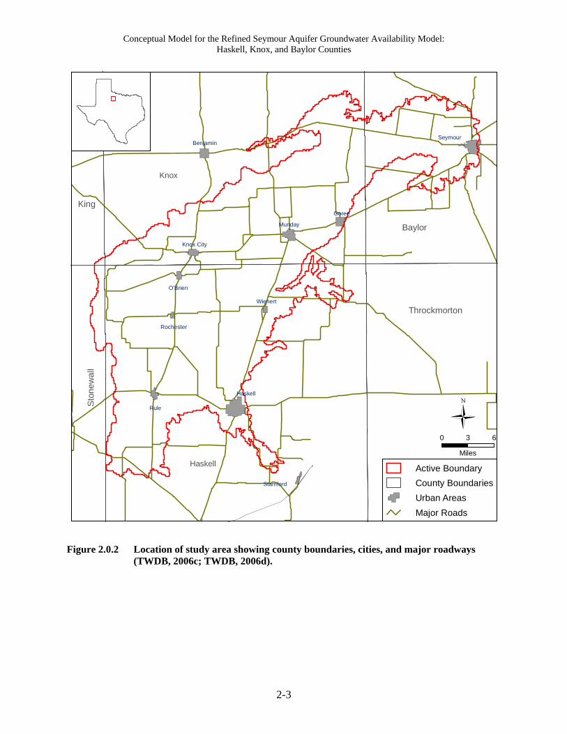
2.0 Study Area
The Seymour Aquifer, as defined by the TWDB (Ashworth and Hopkins, 1995), consists of
isolated pods of unconsolidated alluvium deposits of Quaternary age. The refined Seymour
Aquifer groundwater availability model considers the pod located in Haskell, southern Knox, and
western Baylor counties. The study area and active model boundary for this refined model are
shown in Figure 2.0.1. Figure 2.0.2 shows the counties, roadways, cities, and towns included in
the study area. The locations of rivers, streams, lakes, and reservoirs in the study area are shown
in Figure 2.0.3. The extent of the Seymour Aquifer, the only major or minor aquifer located in
the study area, is shown in Figure 2.0.4. Note that the Seymour Aquifer is exclusively a water-
table aquifer with no subcrop.
Groundwater model boundaries are typically defined on the basis of surface or groundwater
hydrologic boundaries. The lateral boundary of the active model area is defined to include the
entirety of the large Seymour Aquifer pod located in Haskell, southern Knox, and western Baylor
counties. The lateral boundary for the refined model was placed at the edge of the pod or along
Lake Creek or the Brazos River where they fall outside of the pod. This boundary, projected to
plan view, is shown in the report figures as a red solid line and provides the limits of the model
area. Note that not all of the Seymour Aquifer located within the study area (see Figure 2.0.4) is
included in the model area. This is because the objective of the refined model is to model only
the large pod located in Haskell, southern Knox, and western Baylor counties.
The model area encompasses parts of two regional water planning areas (Figure 2.0.5). The
majority of the model area lies within the Brazos G Regional Water Planning Area and a small
portion lies within the Region B Regional Water Planning Area. The model area includes part of
the Rolling Plains Groundwater Conservation District. This is the only Groundwater
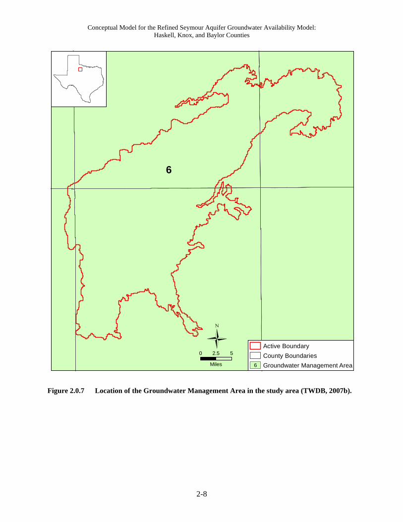
Conservation District located in the model area (Figure 2.0.6). The study area lies within a
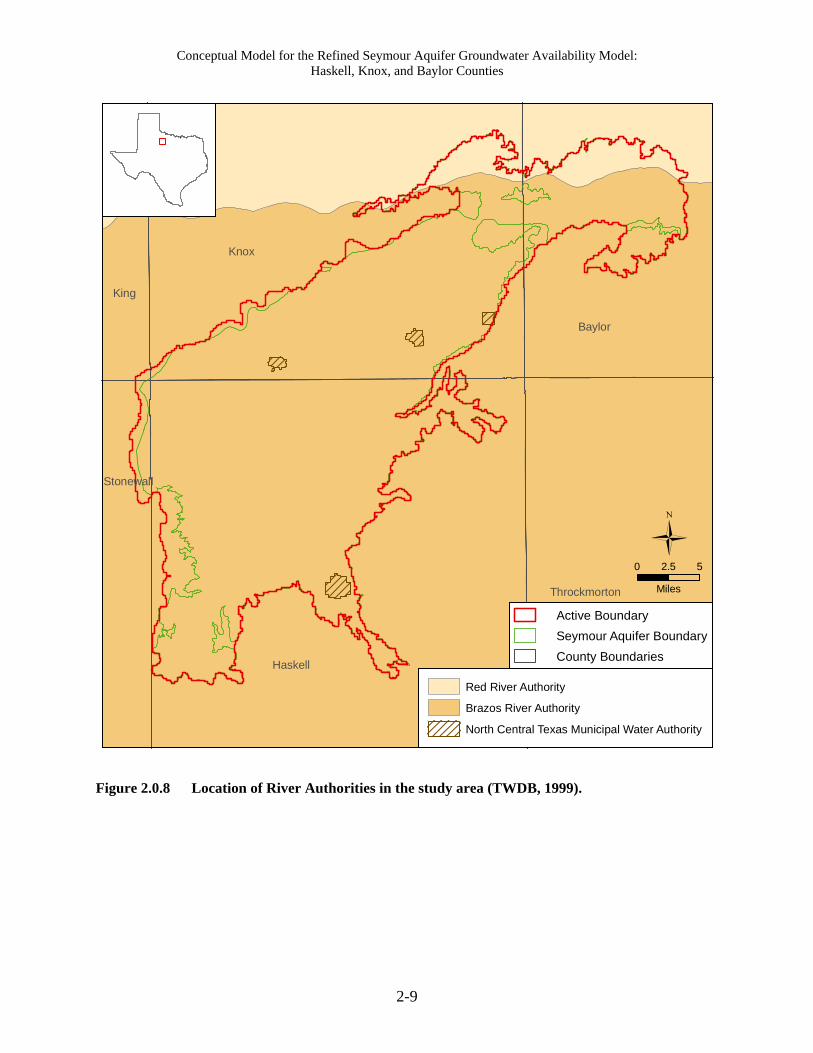
portion of one Groundwater Management Area (Figure 2.0.7). The Brazos River Authority, Red
River Authority, and North Central Texas Municipal Water Authority are found in the study area
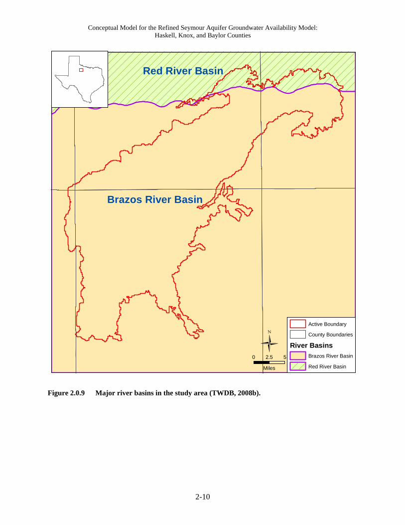
(Figure 2.0.8). The major river basins in the active area are the Red and Brazos river basins
(Figure 2.0.9).

Conceptual Model for the Refined Seymour Aquifer Groundwater Availability Model: Haskell, Knox, and Baylor Counties
2-2
0 10050
Miles
Active Boundary
Study Area
County Boundaries
State Line
Figure 2.0.1 Location of study area and model boundary for the refined Seymour Aquifer groundwater availability model.
Conceptual Model for the Refined Seymour Aquifer Groundwater Availability Model: Haskell, Knox, and Baylor Counties
2-3
Benjamin
Knox City
Haskell
Munday
O'Brien
Rochester
Wienert
Goree
Seymour
Rule
Stamford
Knox
King
Haskell
Sto
ne
wa
ll
Throckmorton
Baylor
0 3 6
Miles
Active Boundary
County Boundaries
Urban Areas
Major Roads
Figure 2.0.2 Location of study area showing county boundaries, cities, and major roadways (TWDB, 2006c; TWDB, 2006d).

Conceptual Model for the Refined Seymour Aquifer Groundwater Availability Model: Haskell, Knox, and Baylor Counties
2-4
Lake Stamford
Millers Creek Reservoir
Lake Davis
King
Knox
Baylor
Haskell
Sto
ne
wa
ll
Throckmorton
0 2.5 5
Miles
Streams & Rivers
Lakes & Reservoirs
Seymour Aquifer Boundary
Active Boundary
County Boundaries
Lake
Cre
ek
Brazos River
Brazo
sRiver
Figure 2.0.3 Location of study area showing lakes and rivers (TWDB, 2007a; Alexander and others, 1999).

Conceptual Model for the Refined Seymour Aquifer Groundwater Availability Model: Haskell, Knox, and Baylor Counties
2-5
King
Knox
Baylor
Haskell
Sto
ne
wa
ll
Throckmorton
0 2.5 5
Miles
Seymour Aquifer
Active Boundary
County Boundaries
Figure 2.0.4 Areal extent of major aquifers in the study area (TWDB, 2006a).

Conceptual Model for the Refined Seymour Aquifer Groundwater Availability Model: Haskell, Knox, and Baylor Counties
2-6
0 3 6
Miles
Active Boundary
County Boundaries
Regional Water Planning AreaBrazos G
Region B
Brazos G
Region B
Region B
Figure 2.0.5 Locations of Regional Water Planning Areas in the study area (TWDB, 2008a).

Conceptual Model for the Refined Seymour Aquifer Groundwater Availability Model: Haskell, Knox, and Baylor Counties
2-7
0 2.5 5
Miles
Active Boundary
County Boundaries
Groundwater Conservation District
Rolling Plains
Rolling Plains
Figure 2.0.6 Location of the Groundwater Conservation District in the study area from the October 2008 Groundwater Conservation District map (TWDB, 2009a).
Conceptual Model for the Refined Seymour Aquifer Groundwater Availability Model: Haskell, Knox, and Baylor Counties
2-8
0 2.5 5
Miles
Active Boundary
County Boundaries
Groundwater Management Area
6
6
Figure 2.0.7 Location of the Groundwater Management Area in the study area (TWDB, 2007b).
Conceptual Model for the Refined Seymour Aquifer Groundwater Availability Model: Haskell, Knox, and Baylor Counties
2-9
Knox
King
Haskell
Stonewall
Throckmorton
Baylor
0 2.5 5
Miles
Active Boundary
Seymour Aquifer Boundary
County Boundaries
Red River Authority
Brazos River Authority
North Central Texas Municipal Water Authority
Figure 2.0.8 Location of River Authorities in the study area (TWDB, 1999).
Conceptual Model for the Refined Seymour Aquifer Groundwater Availability Model: Haskell, Knox, and Baylor Counties
2-10
0 2.5 5
Miles
Active Boundary
County Boundaries
River Basins
Brazos River Basin
Red River Basin
Brazos River Basin
Red River Basin
Figure 2.0.9 Major river basins in the study area (TWDB, 2008b).

Conceptual Model for the Refined Seymour Aquifer Groundwater Availability Model: Haskell, Knox, and Baylor Counties
2-11
2.1 Physiography and Climate
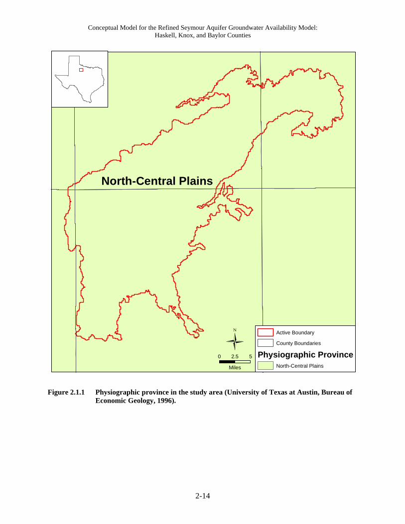
The study area is located completely within the North-Central Plains physiographic province
(Figure 2.1.1). The North-Central Plains are "an erosional surface that developed on upper
Paleozoic formations…" (Wermund, 1996). This province consists of local prairies as well as
hills and rolling plains. The topography is characterized by low north-south trending ridges.
The geologic structure is predominantly a westward dip with minor faults. The bedrock types for
the North-Central Plains province are limestone, sandstone, and shale.
The study is located completely within the Rolling Plains ecological region (Texas Parks and
Wildlife, 2009) (Figure 2.1.2). Together with the High Plains region, the Rolling Plains
represent the southern end of the Great Plains of the central United States. This region originally
consisted of grassland or savannah communities that, due to over grazing by domestic livestock
and a reduction in natural fires, changed to predominately brushland and woodland habitats
(Texas Parks and Wildlife, 2007). The region has also been impacted by the expansion of honey
mesquite in the study area, which has increased erosion and decreased water absorption (Texas
Parks and Wildlife, 2007). Much of the flat terrain within the region has been developed for
agricultural purposes.
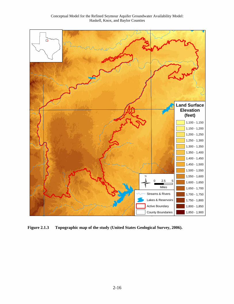
Figure 2.1.3 provides a topographic map of the study area. Generally, the surface elevation
decreases from the southern portion of the Seymour Aquifer pod to the northeastern portion of
the pod. The ground-surface elevation within the model boundaries varies from a high of about
1,700 feet above sea level in Haskell County to a low of about 1,240 feet above sea level just
south of the Brazos River in Baylor County.
The climate in the active model area is classified as the Subtropical Subhumid subcategory of the
Modified Marine or Subtropical climate. (Larkin and Bomar, 1983) (Figure 2.1.4). Larkin and
Bomar (1983) state that "A marine climate is caused by the predominant onshore flow of tropical
maritime air from the Gulf of Mexico. The onshore flow is modified by a decrease in moisture
content from east to west and by intermittent seasonal intrusions of continental air". The
Subhumid category of the Subtropical climate is characterized by hot summers and dry winters
(Larken and Bomar, 1983). In general, most rainfall occurs during the growing season from

Conceptual Model for the Refined Seymour Aquifer Groundwater Availability Model: Haskell, Knox, and Baylor Counties
2-12
April through October. Often, rainfall is heavy over short periods of time. This leads to
occasional flooding and significant periods of drought. A severe drought was experienced in the
study area in the 1950s.
Figure 2.1.5 shows that the mean annual temperature in the study area ranges from a high of
about 65 degrees Fahrenheit in the east to a low of about 63 degrees Fahrenheit in the west
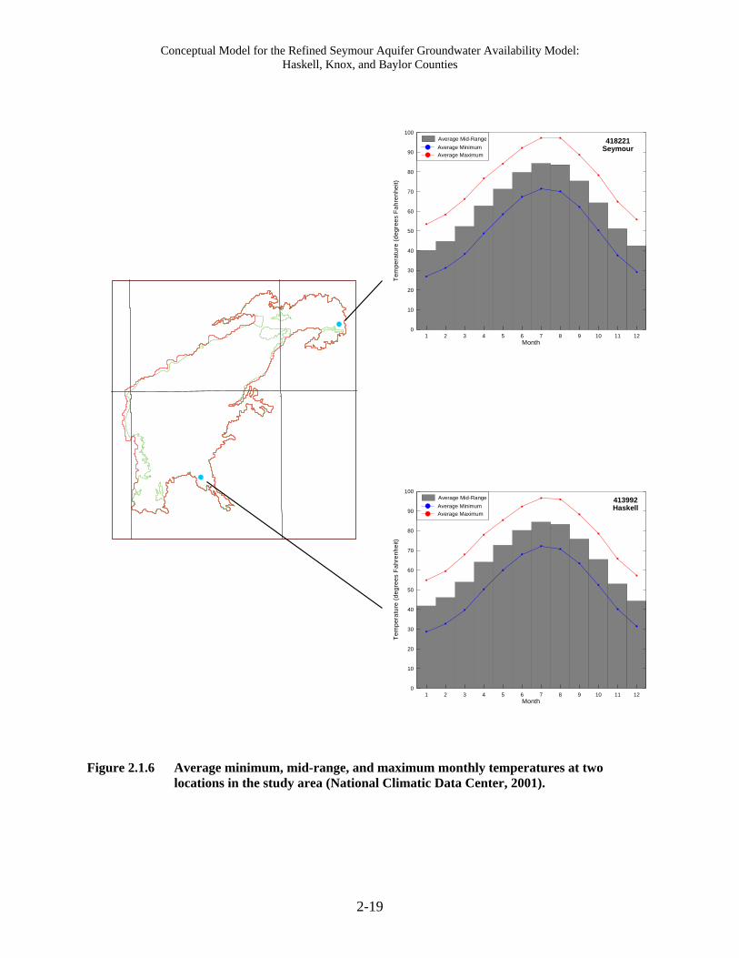
(Texas A&M University, 2002). Monthly variations in temperature are shown in Figure 2.1.6 for
two locations in the study area. This figure shows monthly average mid-range, average
maximum, and average minimum temperatures. These monthly temperatures were calculated by
first averaging minimum and maximum daily temperatures from the National Climatic Data
Center to get average monthly values. This was done for every month from January 1948
through August 2002. For each month, the average minimum and maximum values for all the
years were then averaged to obtained the monthly average mid-range values shown in
Figure 2.1.6.
Figure 2.1.7 shows that precipitation data are available at 13 stations in the study area (National
Climatic Data Center, 2001). Measurement of precipitation at most gages began in the 1940s. In
general, measurements are not continuous on a month-by-month or year-by-year basis for the
gages. Annual precipitation recorded at two stations within the model area is shown in Figure
2.1.8. Figure 2.1.9 provides a raster data post plot of the Parameter-Elevation Regressions on
Independent Slopes Model (Oregon State University, 2002) of average annual precipitation
across the study area based on data for the period from 1971 to 2000. Generally, the average
annual precipitation decreases from a high of about 27.5 inches per year in the east to a low of
about 24.5 inches per year in the west.
The average annual net pan evaporation rate in the study area ranges from a high of 99 inches per
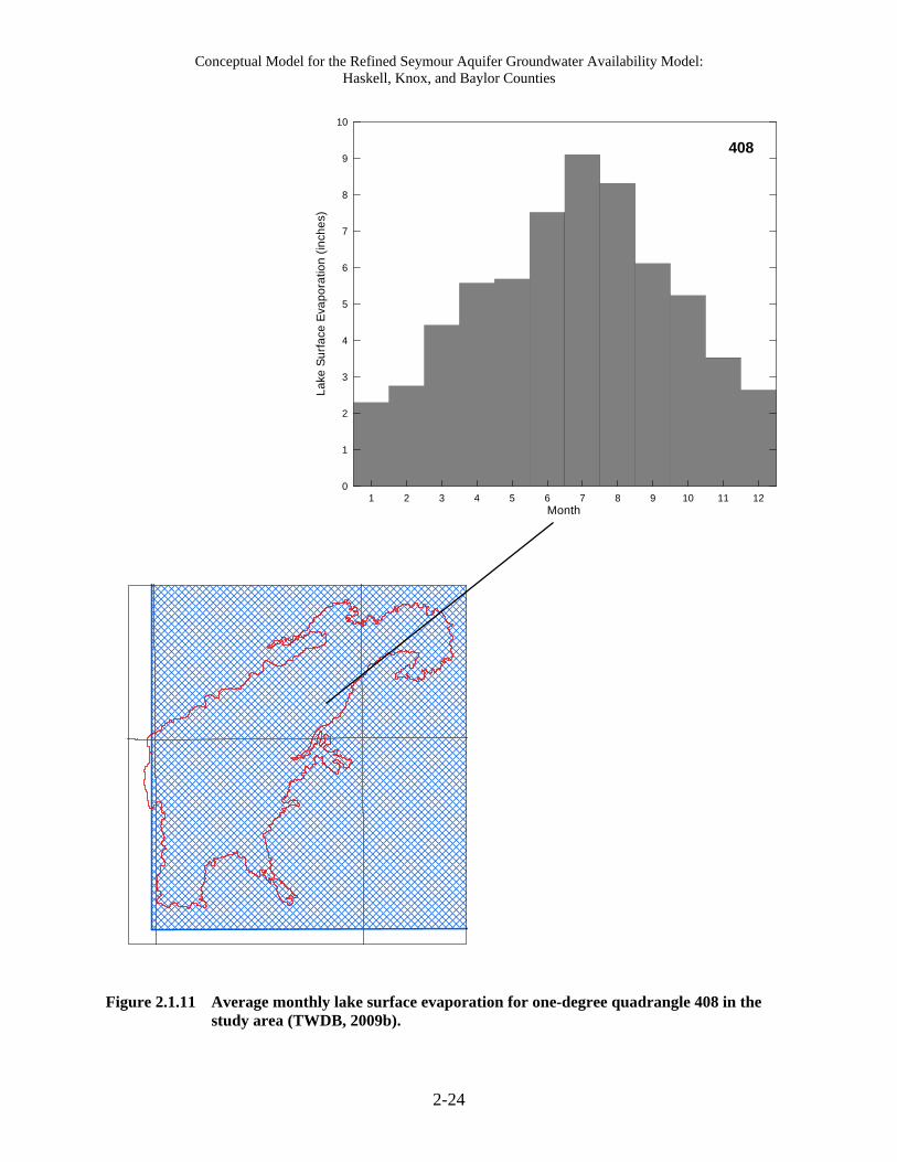
year to a low of 90 inches per year (Figure 2.1.10). The majority of the model area falls within
one-degree quadrangle 408, which has an average annual net pan evaporation rate of 92 inches
per year. The pan evaporation rate significantly exceeds the annual average rainfall. The
greatest rainfall deficit of about 68 inches per year occurs along the western side of the model
area. Monthly variations in lake surface evaporation are shown in Figure 2.1.11 for one-degree
quadrangle 408. These values represent the average of the monthly lake surface evaporation data

Conceptual Model for the Refined Seymour Aquifer Groundwater Availability Model: Haskell, Knox, and Baylor Counties
2-13
for January 1954 through December 2004 (TWDB, 2009b). The annual average lake surface
evaporation rate is about 63 inches per year for one-degree quadrangle 408. Potential
evapotranspiration, a measure of the ability of the atmosphere to remove water from ground
surface by evaporation and transpiration assuming an infinite water supply, ranges from a low of
about 63.5 inches per year to a high of about 67 inches per year in the study area (Figure 2.1.12).
Conceptual Model for the Refined Seymour Aquifer Groundwater Availability Model: Haskell, Knox, and Baylor Counties
2-14
0 2.5 5
Miles
Active Boundary
County Boundaries
Physiographic ProvinceNorth-Central Plains
North-Central Plains
Figure 2.1.1 Physiographic province in the study area (University of Texas at Austin, Bureau of Economic Geology, 1996).

Conceptual Model for the Refined Seymour Aquifer Groundwater Availability Model: Haskell, Knox, and Baylor Counties
2-15
0 2.5 5
Miles
Active Boundary
County Boundaries
Ecological Region
Rolling Plains
Rolling Plains
Figure 2.1.2 Ecological region in the study area (Texas Parks and Wildlife, 2009).
Conceptual Model for the Refined Seymour Aquifer Groundwater Availability Model: Haskell, Knox, and Baylor Counties
2-16
0 2.5 5
MilesStreams & Rivers
Lakes & Reservoirs
Active Boundary
County Boundaries
Land SurfaceElevation
(feet)
1,100 - 1,150
1,150 - 1,200
1,200 - 1,250
1,250 - 1,300
1,300 - 1,350
1,350 - 1,400
1,400 - 1,450
1,450 - 1,500
1,500 - 1,550
1,550 - 1,600
1,600 - 1,650
1,650 - 1,700
1,700 - 1,750
1,750 - 1,800
1,800 - 1,850
1,850 - 1,900
Figure 2.1.3 Topographic map of the study (United States Geological Survey, 2006).

Conceptual Model for the Refined Seymour Aquifer Groundwater Availability Model: Haskell, Knox, and Baylor Counties
2-17
0 2.5 5
Miles
Subtropical Subhumid Climate
Active Boundary
County Boundaries
SubtropicalSubhumid
Figure 2.1.4 Climate classification in the study area (Larkin and Bomar, 1983).

Conceptual Model for the Refined Seymour Aquifer Groundwater Availability Model: Haskell, Knox, and Baylor Counties
2-18
0 2 4
Miles
Active Boundary
County Boundaries
Mean Annual Temperature
62 - 64 degrees Fahrenheit
64 - 66 degrees Fahrenheit
64 - 66
62 - 64
Figure 2.1.5 Average annual air temperature in the study area (Texas A&M University, 2002).
Conceptual Model for the Refined Seymour Aquifer Groundwater Availability Model: Haskell, Knox, and Baylor Counties
2-19
!
!
1 2 3 4 5 6 7 8 9 10 11 12Month
0
10
20
30
40
50
60
70
80
90
100
Te
mp
era
ture
(d
eg
ree
s F
ah
ren
he
it)
Average Mid-Range
Average Minimum
Average Maximum
413992Haskell
1 2 3 4 5 6 7 8 9 10 11 12Month
0
10
20
30
40
50
60
70
80
90
100
Te
mp
era
ture
(d
eg
ree
s F
ah
ren
he
it)
Average Mid-Range
Average Minimum
Average Maximum
418221Seymour
Figure 2.1.6 Average minimum, mid-range, and maximum monthly temperatures at two locations in the study area (National Climatic Data Center, 2001).

Conceptual Model for the Refined Seymour Aquifer Groundwater Availability Model: Haskell, Knox, and Baylor Counties
2-20
!
!
!
!
!
!
!
!
! !
!!! !
King
Knox
Baylor
Haskell
Sto
ne
wa
ll
Throckmorton
418221417499417769
410708
417572410704
416146
414852
416148
419013
413994
413992
413995
0 2.5 5
Miles
Precipitation Gage
! 413992
Active Boundary
County Boundaries
Figure 2.1.7 Location of precipitation gages in the study area (National Climatic Data Center, 2001).

Conceptual Model for the Refined Seymour Aquifer Groundwater Availability Model: Haskell, Knox, and Baylor Counties
2-21
!
!
1930 1940 1950 1960 1970 1980 1990 2000Year
0
5
10
15
20
25
30
35
40
45
50
55
An
nu
al P
reci
pita
tion
(in
che
s p
er
yea
r)
Mean = 26.42 inches per year
418221Baylor
1930 1940 1950 1960 1970 1980 1990 2000Year
0
5
10
15
20
25
30
35
40
45
50
55
An
nu
al P
reci
pita
tion
(in
che
s p
er
yea
r)
Mean = 24.83 inches per year
413992Haskell
Figure 2.1.8 Annual precipitation time series at two locations in the study area (National
Climatic Data Center, 2001). (A discontinuous line indicates a break in the data. The dashed red line represents the mean annual precipitation.)

Conceptual Model for the Refined Seymour Aquifer Groundwater Availability Model: Haskell, Knox, and Baylor Counties
2-22
0 2.5 5
Miles
Active Boundary
County Boundaries
Precipitation(inches per year)
24.0 - 24.5
24.6 - 25.0
25.1 - 25.5
25.6 - 26.0
26.1 - 26.5
26.6 - 27.0
27.1 - 27.5
27
24.5
25
25.5
2626.5
26
Figure 2.1.9 Average annual precipitation over the study area (Oregon State University, 2002).

Conceptual Model for the Refined Seymour Aquifer Groundwater Availability Model: Haskell, Knox, and Baylor Counties
2-23
King
Knox
Baylor
Haskell
Sto
ne
wa
ll
Throckmorton9299
9091
0 2.5 5
Miles
Active Boundary
County Boundaries
Net Pan EvaporationRate (inches per year)
90
91
92
99
Figure 2.1.10 Average annual net pan evaporation over the study area (TWDB, 2009b).
Conceptual Model for the Refined Seymour Aquifer Groundwater Availability Model: Haskell, Knox, and Baylor Counties
2-24
DDDDDDDDDDDDDDDDDDDDDDDDDDDDDDDDDDDDDDDDDDDDDDDDDDDDDDDDDDDDDDDDDDDDDDDDDDDDDDDDDDDDDDDDDDDDDDDDDDDDDDDDDDDDDDDDDDDDDDDDDDDDDDDDDDDDDDDDDDDDDDDDDDDDDDDDDDDDDDDDDDDDDDDDDDDDDDDDDDDDDDDDDDDDDDDDDDDDDDDDDDDDDDDDDDDDDDDDDDDDDDDDDDDDDDDDDDDDDDDDDDDDDDDDDDDDDDDDDDDDDDDDDDDDDDDDDDDDDDDDDDDDDDDDDDDDDDDDDDDDDDDDDDDDDDDDDDDDDDDDDDDDDDDDDDDDDDDDDDDDDDDDDDDDDDDDDDDDDDDDDDDDDDDDDDDDDDDDDDDDDDDDDDDDDDDDDDDDDDDDDDDDDDDDDDDDDDDDDDDDDDDDDDDDDDDDDDDDDDDDDDDDDDDDDDDDDDDDDDDDDDDDDDDDDDDDDDDDDDDDDDDDDDDDDDDDDDDDDDDDDDDDDDDDDDDDDDDDDDDDDDDDDDDDDDDDDDDDDDDDDDDDDDDDDDDDDDDDDDDDDDDDDDDDDDDDDDDDDDDDDDDDDDDDDDDDDDDDDDDDDDDDDDDDDDDDDDDDDDDDDDDDDDDDDDDDDDDDDDDDDDDDDDDDDDDDDDDDDDDDDDDDDDDDDDDDDDDDDDDDDDDDDDDDDDDDDDDDDDDDDDDDDDDDDDDDDDDDDDDDDDDDDDDDDDDDDDDDDDDDDDDDDDDDDDDDDDDDDDDDDDDDDDDDDDDDDDDDDDDDDDDDDDDDDDDDDDDDDDDDDDDDDDDDDDDDDDDDDDDDDDDDDDDDDDDDDDDDDDDDDDDDDDDDDDDDDDDDDDDDDDDDDDDDDDDDDDDDDDDDDDDDDDDDDDDDDDDDDDDDDDDDDDDDDDDDDDDDDDDDDDDDDDDDDDDDDDDDDDDDDDDDDDDDDDDDDDDDDDDDDDDDDDDDDDDDDDDDDDDDDDDDDDDDDDDDDDDDDDDDDDDDDDDDDDDDDDDDDDDDDDDDDDDDDDDDDDDDDDDDDDDDDDDDDDDDDDDDDDDDDDDDDDDDDDDDDDDDDDDDDDDDDDDDDDDDDDDDDDDDDDDDDDDDDDDDDDDDDDDDDDDDDDDDDDDDDDDDDDDDDDDDDDDDDDDDDDDDDDDDDDDDDDDDDDDDDDDDDDDDDDDDDDDDDDDDDDDDDDDDDDDDDDDDDDDDDDDDDDDDDDDDDDDDDDDDDDDDDDDDDDDDDDDDDDDDDDDDDDDDDDDDDDDDDDDDDDDDDDDDDDDDDDDDDDDDDDDDDDDDDDDDDDDDDDDDDDDDDDDDDDDDDDDDDDDDDDDDDDDDDDDDDDDDDDDDDDDDDDDDDDDDDDDDDDDDDDDDDDDDDDDDDDDDDDDDDDDDDDDDDDDDDDDDDDDDDDDDDDDDDDDDDDDDDDDDDDDDDDDDDDDDDDDDDDDDDDDDDDDDDDDDDDDDDDDDDDDDDDDDDDDDDDDDDDDDDDDDDDDDDDDDDDDDDDDDDDDDDDDDDDDDDDDDDDDDDDDDDDDDDDDDDDDDDDDDDDDDDDDDDDDDDDDDDDDDDDDDDDDDDDDDDDDDDDDDDDDDDDDDDDDDDDDDDDDDDDDDDDDDDDDDDDDDDDDDDDDDDDDDDDDDDDDDDDDDDDDDDDDDDDDDDDDDDDDDDDDDDDDDDDDDDDDDDDDDDDDDDDDDDDDDDDDDDDDDDDDDDDDDDDDDDDDDDDDDDDDDDDDDDDDDDDDDDDDDDDDDDDDDDDDDDDDDDDDDDDDDDDDDDDDDDDDDDDDDDDDDDDDDDDDDDDDDDDDDDDDDDDDDDDDDDDDDDDDDDDDDDDDDDDDDDDDDDDDDDDDDDDDDDDDDDDDDDDDDDDDDDDDDDDDDDDDDDDDDDDDDDDDDDDDDDDDDDDDDDDDDDDDDDDDDDDDDDDDDDDDDDDDDDDDDDDDDDDDDDDDDDDDDDDDDDDDDDDDDDDDDDDDDDDDDDDDDDDDDDDDDDDDDDDDDDDDDDDDDDDDDDDDDDDDDDDDDDDDDDDDDDDDDDDDDDDDDDDDDDDDDDDDDDDDDDDDDDDDDDDDDDDDDDDDDDDDDDDDDDDDDDDDDDDDDDDDDDDDDDDDDDDDDDDDDDDDDDDDDDDDDDDDDDDDDDDDDDDDDDDDDDDDDDDDDDDDDDDDDDDDDDDDDDDDDDDDDDDDDDDDDDDDDDDDDDDDDDDDDDDDDDDDDDDDDDDDDDDDDDDDDDDDDDDDDDDDDDDDDDDDDDDDDDDDDDDDDDDDDDDDDDDDDDDDDDDDDDDDDDDDDDDDDDDDDDDDDDDDDDDDDDDDDDDDDDDDDDDDDDDDDDDDDDDDDDDDDDD
1 2 3 4 5 6 7 8 9 10 11 12Month
0
1
2
3
4
5
6
7
8
9
10
La
ke S
urf
ace
Eva
po
ratio
n (
inch
es)
408
Figure 2.1.11 Average monthly lake surface evaporation for one-degree quadrangle 408 in the study area (TWDB, 2009b).

Conceptual Model for the Refined Seymour Aquifer Groundwater Availability Model: Haskell, Knox, and Baylor Counties
2-25
King
Knox
Baylor
Haskell
Stonewall
Throckmorton
0 2.5 5
Miles
Active Boundary
County Boundaries
PotentialEvapotranspiration(inches per year)
High : 66.9971
Low : 63.5834
Figure 2.1.12 Potential evapotranspiration in the study area (Borrelli and others, 1998).

Conceptual Model for the Refined Seymour Aquifer Groundwater Availability Model: Haskell, Knox, and Baylor Counties
2-26
This page is intentionally blank.

Conceptual Model for the Refined Seymour Aquifer Groundwater Availability Model: Haskell, Knox, and Baylor Counties
2-27
2.2 Geology
The structural setting for the study area is shown in Figure 2.2.1. In the subsurface, the area is
characterized by the Baylor Syncline, which was formed during Pennsylvanian time (Price,
1979). Structural deformation of the Baylor Syncline has no affect on the Seymour Aquifer.
The surface geology in the study area (Figure 2.2.2) consists of Permian- through Quaternary-
aged deposits. The Quaternary-age deposits making up the Seymour Aquifer overlie Permian-
age deposits. From oldest to youngest and east to west, the Permian-age deposits form the
Wichita Group, the Clear Fork Group, and the Pease River Group. Table 2.2.1 summarizes the
geologic units in the study area. A schematic of the stratigraphy in the study area is provided in
Figure 2.2.3.
The following geologic history of the study area is taken primarily from Preston (1978). Shallow
seas covered the study area from the Cambrian Period through the Permian Period. During the
early time period (Cambrian through Mississippian), these seas were calm resulting in the
deposition of limestone and shales characteristic of a stable environment with long periods of
deposition. During the later Pennsylvanian and Permian periods, the relatively calm seas were
replaced by "continued rapid transgression and regression of shallow epicontinental seas"
(Preston, 1978). This resulted in "thick sequences of relatively thin-bedded deposits of almost
every type of depositional environment from shallow-shelf, through deltaic, fluvial, and
continental" (Preston, 1978). Deposits of the Permian Period dip to the west-northwest at about
20 to 40 feet per mile (Ogilbee and Osborne, 1962; Preston, 1978). A major erosional
unconformity exists between the Permian and overlying Quaternary-age deposits in the study
area. Therefore, no depositional record is available for that time period. The surface of the
Permian-age deposits shows well-developed drainage patterns indicating a long period of erosion
(R.W. Harden and Associates, 1978).
All material forming the Seymour Aquifer are unconsolidated alluvial sediments of non-marine
origin deposited on the erosional surface of Permian-age beds. In general, sediments of the
Seymour Aquifer are predominately material eroded from the High Plains and deposited by
eastward moving streams (R.W. Harden and Associates, 1978; Nordstrom, 1991; Duffin and

Conceptual Model for the Refined Seymour Aquifer Groundwater Availability Model: Haskell, Knox, and Baylor Counties
2-28
Beynon, 1992). It is likely that the sediments originally blanketed the entire region where the
Seymour Aquifer is found, but were subsequently eroded by recent streams, leaving only
remnants of the once continuous deposits (Ogilbee and Osborne, 1962; Preston, 1978; Price
1978). These remnants, along with younger windblown, terrace, and surficial deposits, make up
the Seymour Aquifer (see Figure 2.2.2).
Sediments of the Seymour Aquifer in the study area are composed of clay, silt, sand,
conglomerate, gravel, and some caliche and volcanic ash (Ogilbee & Osborne, 1962). In
general, the sediments are finer near the top and coarsen with depth. The upper portion contains
beds of fine-grained sand with silt or clay and caliche in some locations. Where found, the
caliche is typically located 1 to 2 feet below ground surface. A basal section of coarse sand and
gravel beds is present in many portions of the aquifer in the study area. Individual beds within
the Seymour aquifer are discontinuous and grade laterally into beds of coarser or finer grained
material. The thickness of the Seymour Aquifer in the study area varies from 0 to about 110 feet.
This variation is due to the uneven erosional surface of the Seymour Aquifer and the underlying
Permian-age deposits. Where the aquifer overlies a buried channel, it typically has a greater
thickness and an increased amount of coarse material at its base. Where the aquifer is thin, it
consists predominantly of finer-grained material.
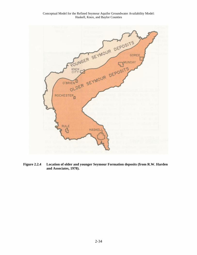
R.W. Harden and Associates (1978) indicate that the Seymour Formation in Haskell and
southern Knox counties can be divided into older deposits in the south and east and younger
deposits in the north and west (Figure 2.2.4). The distinction between these sediments is a small
topographic break. R.W. Harden and Associates (1978) state that
"The break represents an episode of valley deepening which was followed subsequently
by alluviation. The younger deposits occur beneath a terrace extending along the
northern and northwestern edge of the area in a belt approximately 4 miles wide."
Several cross-sections through the portion of the Seymour Aquifer in Haskell and Knox counties
studied by R.W. Harden and Associates (1978) are shown in Figures 2.2.5 and 2.2.6. These
cross-sections, taken directly from their report, show the relationship between the Seymour
Formation and the underlying Clear Fork Group. These cross-sections also show the location of
the water table in 1977. Figure 2.2.7 shows a cross-section through the Seymour Formation in

Conceptual Model for the Refined Seymour Aquifer Groundwater Availability Model: Haskell, Knox, and Baylor Counties
2-29
Baylor County. This cross-section provides a good illustration of the sediment types found in the
Seymour Aquifer.

Conceptual Model for the Refined Seymour Aquifer Groundwater Availability Model: Haskell, Knox, and Baylor Counties
2-30
Table 2.2.1 Rock units in the study area (after United States Geological Survey-Texas Water Science Center and the Texas Natural Resources Information System, 2004).
Rock Unit Code
Rock Unit Name Group Period General Description
Qal Alluvium na Quaternary floodplain and channel deposits of sand, silt, clay and gravel
Qds Windblown deposits: dunes and dune ridges
na Quaternary massive sand and silt with local low-angle crossbeds
Qsh Windblown deposits: sheet deposits
na Quaternary laminated silt and sand derived from nearby windblown accumulations
Qp Playa lake deposits na Quaternary lenticular, laminated, and desiccation-cracked clay and laminated silt and sand deposited principally on margins of playas
Qt Fluviatile terrace deposits
na Quaternary
sandy, lenticular, stratified, and cross bedded gravel with local calcite cement; laminated and crossbedded, fine- to coarse-grained sand; sandy/clayey silt bedded and lenticular; a veneer of windblown sand and silt covers upper terrace levels
Qs Seymour Formation: thin deposits
na Quaternary silty sand with tiny gravel in basal part; generally massive to crudely stratified; locally cemented by calcite; some well developed caliche
Qs2 Seymour Formation: thick deposits
na Quaternary
predominately gravel and thick-bedded, massive, silty sand with minor lenticular clay beds; well-developed caliche near the surface; basal lenticular, sandy, granule- to boulder-size gravel locally cemented with calcite
Qu Surficial deposits undivided
na Quaternary
sand, clay, silt, caliche, and gravel; includes thin remnants of older terraces and of Seymour Formation, lag gravel, windblown sand and silt, residual soil, and colluvium commonly cemented by caliche
Pb Blaine Formation Pease River
Permian mudstone, gypsum, dolomite, and sandstone with the dolomite beds laterally persistent and predominant
Psa San Angelo Formation
Pease River
Permian predominantly mudstone and siltstone with thin lenses of gypsum in the upper portion and very fine to fine grained sandstone in the lower portion
Pcf Clear Fork undivided
Clear Fork
Permian predominately mudstone with thin beds of siltstone sandstone, dolomite, and limestone
Pl Lueders Formation Wichita Permian massive to thin beds of limestone interbedded with dolomite and shale
Pt Talpa Formation Wichita Permian predominantly shale with some limestone beds
Pgc Grape Creek Formation
Wichita Permian thick-bedded shale with thin lentils of argillaceous limestone and calcareous siltstone
Pbe Bead Mountain Formation
Wichita Permian predominantly shale with local limestone lentils in the upper portion and predominantly limestone with thin shale interbeds in the lower portion

Conceptual Model for the Refined Seymour Aquifer Groundwater Availability Model: Haskell, Knox, and Baylor Counties
2-31
0 2.5 5
Miles
Active Boundary
County Boundaries
Structural Features
Baylor Syncline
Figure 2.2.1 Major structural features in the study area (Price, 1979).

Conceptual Model for the Refined Seymour Aquifer Groundwater Availability Model: Haskell, Knox, and Baylor Counties
2-32
Knox
King
Haskell
Stonewall
Throckmorton
Baylor
Pcf
Pcf
Pl
Qs2
Qsh
Qs
Pjv
Pl
Pcf
Psa
Pt
Pb
Qal
QuPgc
Qs2
Pl
Pcf
Pbe
Qal
Pbe
Qal
Qt
Qt
Qal
Pbe
Psa
Qs2
Psa
Psa
Qal
Pcf
Qds
Qs Qu
Qu
Qsh
Pcf
Psa
Wa
Qt
Pcf
Qt
Qs2
Qu
Qt
Qu
Qu
Pl
Qu
Qt
Qds
QuQu
Qt
Qg
Qt
Qt
Qsh
Qds
Qs2
Qt
Qg
Pb
Qds
Qt
Pcf
Qt
Qg
Qs2
Qt
Qu
Qu
Pt
Qt
Qt
Qt
Qt
Qt
Qg
Qu
Qg
Qt
Qal
Qu
Qu
Pt
Qal
Qal
Wa
Qal
Qal
Qu
Pt
Qal
Qt
Pt
Qal
Pcf
Qs2
Pl
Qal
Qu
Qt
Qt
Qal
Qal
Qu
Pcf
Qu
Pcf
Qu
Pl
Qal
Pgc
Qt
Pcf
Qt
Qal
Qt
Pcf
Qt
Qds
Qal
Qu
Psa
Qt
Pcf
Qal
Qu
Qal
Qt
Qt
Qt
Pgc
Qu
Qal
Pcf
QtQds
Wa
Qt
Qg
Qal
Qu
Qp
Qal
Qt
Qt
Pcf
Qds
Wa
Qal
Qt
Qal
Qt
Pcf
Qt
Qds
Qp
Qt
Qds
Qt
Qp
Qal
Pb
Pl
Qt
Qal
Pb
Pcf
Qt Qt
Qt
Pl
Qal
Pbe
Qt
Qt
Pcf
Qp
Qt
Qu
Qt
Qal
Qu
Qt
Qt
Qal
Pl
Qg
Qt
QtPgc
Qt
Qt
Pjv
Qt
Qg
Qds
Qg
Qt
Pl
Pb
Qt
Qal
Qt
Pcf
Qal
Pbe
Qsh
Pcf
QtPgc
Pl
Qt
Pcf
Qg
Qt
Qt
Qal
Pl
Pt
Qu
Pl
Qt
Qp
Qp
Qal
Qp
Qt
Qal
Qt
Qt
Qt
Pgc
Pgc
Qt
Psa
Qt
Pcf
Pcf
Pl
Qt
Wa
Qp
Qu
Qt
Qt
Qt
Pl
Qt
Qt
Qp
Qt
Pcf
Qt
Qp
Qp
Qt
Pcf
Qt
Qg
Qds
QdsQds
Pl
Qp
Pcf
Qt
Qt
Pcf
Psa
Pjv
Pcf
Qt
Qt
Qds
QuQt
Qg
Pbe
Qal
Qp
Qp
Pcf
Qp
Pgc
Wa
Pl
Qp
Pl
Pcf
Pl
Qt
Qt
Qt
Pl
Pl
Qal
Qds
Qp
Pcf
Qg
Pjv
Pcf
PjvPbe
PcfQg
Wa
Wa
Pl
Qu
Pcf
Pl
Pgc
Pjv
Qg
Psa
Pcf
Qs2
Pgc
Pt
Pl
Pjv
Pcf
Pjv
Pjv
Wa
Pt
Pt
Psa
Pgc
Psa
Pl
Wa
Pt
Pt
Pt Pjv
Pl
Pbe
Pjv
Pl
Pcf
Pb
Pcf
Qg
Pl
PlPt
Pcf
Pbe
0 2.5 5
Miles
County Boundaries
Active Boundary
Seymour Aquifer Boundary
Rock Unit
Qu-surficial
Qt-terrace
Qsh-windblown (sheet)
Qs2-Seymour (thick)
Qs-Seymour (thin)
Qp-playa lake deposits
Qds-windblown (dunes)
Qal-alluvium
Pbe-Bead Mountain
Pgc-Grape Creek
Pt-Talpa
Pl-Lueders
Pcf-Clear Fork
Psa-San Angelo
Pb-Blaine
Wa-Water
Pb
Qs2
Qs2
Pcf
Pcf
Pcf
Pcf
Pcf
Pcf
Pl
Qal
Pl
PbeQal
Pt
Pt
Pgc
Figure 2.2.2 Surface geology of the study area (United States Geological Survey-Texas Water Science Center and the Texas Natural Resources Information System, 2004).

Conceptual Model for the Refined Seymour Aquifer Groundwater Availability Model: Haskell, Knox, and Baylor Counties
2-33
Wichita Group
Seymour
GeologicAge
Clear Fork Group
Pease River Group
Quaternary
Permian
Figure 2.2.3 Schematic of generalized stratigraphy across the study area.
Conceptual Model for the Refined Seymour Aquifer Groundwater Availability Model: Haskell, Knox, and Baylor Counties
2-34
Figure 2.2.4 Location of older and younger Seymour Formation deposits (from R.W. Harden and Associates, 1978).

Conceptual Model for the Refined Seymour Aquifer Groundwater Availability Model: Haskell, Knox, and Baylor Counties
2-35
Knox
King
Haskell
Stonewall
Throckmorton
Baylor
0 2.5 5
Miles
Active Boundary
Seymour Aquifer Boundary
County Boundaries
R.W. Harden and Associates (1978) Seymour Aquifer Boundary
Figure 2.2.5 A-A', B-B', C-C', and D-D' cross-sections from R.W. Harden and Associates (1978) showing the Seymour Formation and Clear Fork Group in Haskell and Knox counties.

Conceptual Model for the Refined Seymour Aquifer Groundwater Availability Model: Haskell, Knox, and Baylor Counties
2-36
Knox
King
Haskell
Stonewall
Throckmorton
Baylor
0 2.5 5
Miles
Active Boundary
Seymour Aquifer Boundary
County Boundaries
R.W. Harden and Associates (1978) Seymour Aquifer Boundary
Figure 2.2.6 E-E', F-F', and G-G' cross-sections from R.W. Harden and Associates (1978) showing the Seymour Formation and Clear Fork Group in Haskell and Knox counties.

Conceptual Model for the Refined Seymour Aquifer Groundwater Availability Model: Haskell, Knox, and Baylor Counties
2-37
A A'!
!! ! !
!
Knox
King
Haskell
Stonewall
Throckmorton
Baylor
AA'
Figure 2.2.7 Geologic cross-section through the Seymour Formation in Baylor County (from Preston, 1978).

Conceptual Model for the Refined Seymour Aquifer Groundwater Availability Model: Haskell, Knox, and Baylor Counties
2-38
This page is intentionally blank.
Conceptual Model for the Refined Seymour Aquifer Groundwater Availability Model: Haskell, Knox, and Baylor Counties
2-39
2.3 Brief Land Use History of Baylor, Knox, and Haskell Counties
Water levels in the Seymour Aquifer have been affected by changes in land use since the arrival
of Anglo residents in Haskell, Knox, and Baylor counties. This section provides a brief history
of land use changes in these three counties. This history was predominately developed based on
information provided in Texas State Historical Association (2008) and Texas Parks and Wildlife
(2007). A discussion of water-level changes in the Seymour Aquifer is provided in
Section 4.3.1.
Initially, Haskell, Knox, and Baylor counties were inhabited by nomadic Indians that used the
region as a hunting ground for bison (Sherrill, 1965). In 1858, all three counties were created by
the Texas legislature; however, they were not populated by Anglos at that time due to the threat
of Indian attacks. Military camps were established in the counties after they were created, but it
was not until the late 1870s, when buffalo herds were decimated by hunters, that the Indians
were driven from the region and settlement of the counties by Anglos began. The first settlers
into the area in the late 1870s were ranchers, quickly followed by farmers. Ranching dominated
the region through the 1880’s. Baylor County was formally organized with a county seat in 1879
and Knox and Haskell counties in 1885. Although ranching was still an important component of
the economy, farming became firmly established in the counties by 1900. The land cover during
this time period was predominately mid and tall grasses (Texas Parks and Wildlife, 2007).
Ansley and others (1997), citing a report from 1854 and another from 1866, indicate that large
mesquite were scattered among Texas rangeland and "honey mesquite was a natural part of the
Texas vegetation complex prior to white settlement". These mesquite were located
predominately in riparian areas and not on open grassland. Wilson and others (2001) suggest
that the absence of mesquite on open range during this time period was due to fires, both natural
and intentionally set by Indians, which "presumably minimized mesquite seedling establishment
in open areas while allowing the continued presence of mesquite in sheltered drainage and
riparian areas".
The replacement of buffalo with cattle and sheep had a significant impact on grazing in these
counties, resulting in a significant change in native vegetation (Texas Parks and Wildlife, 2007).
The migrant buffalo herds would graze down an area in a short period of time, consuming all of

Conceptual Model for the Refined Seymour Aquifer Groundwater Availability Model: Haskell, Knox, and Baylor Counties
2-40
the palatable plants, and then move on leaving the area well fertilized and the soils tilled. Texas
Parks and Wildlife (2007) states that "this type of grazing provided long rest periods to native
grasslands, allowing for rapid responses of annual forbs and grasses". This increased plant
diversity and allowed for the development of stands of dense grasses. The introduction of
fencing and overgrazing by domestic livestock resulted in limited or no rest for pastures,
reducing the desired deep-root grasses and increasing "less desirable shallow-rooted grasses and
a few undesirable forbs" (Texas Parks and Wildlife, 2007). Grazing by domestic livestock also
contributed to the expansion of honey mesquite into open grassland through the dispersal of
mesquite seeds in livestock waste and the lack of herbaceous competition for mesquite seedlings
(Wilson and others, 2001). The introduction of domestic livestock also brought a reduction in
fires due to the elimination of intentionally set fires and the absence of herbaceous fuel to
support natural fires. In summary, the switch from buffalo grazing to domestic livestock
grazing, combined with the reduction in fires in the counties, caused “an increase in woody plant
species and a change from grassland or savannah communities to more brushland or woodland
habitat types" (Texas Parks and Wildlife, 2007) and the expansion of woody species, especially
honey mesquite, on open grassland. In addition to expanding the range of honey mesquite,
heavy grazing was also detrimental to the surface soil resulting in decreased infiltration of
precipitation and increased soil erosion (Warren and others, 1986; Wilcox and others, 2008).
All three counties saw an increase in economic development from about 1900 to 1910 due to the
introduction of railroads and a cotton boom. An increase in agriculture due to the cotton boom
and to the selling of ranchland to farmers was also seen in this period. Baylor County
experienced its largest population in 1910. The economic development slowed from about 1910
to 1920 due to droughts and falling crop prices during and after World War 1. A second
economic boom was experience in these three counties from about 1920 to 1930 due
predominately to a brief, intense cotton boom. According to the information available in the
Texas State Historical Association (2008), the acreage used for agricultural purposes in these
counties was greatest during this time period and Haskell and Knox counties experienced their
largest population in 1930. Expansion in all three counties ended in the 1930s and farming
suffered severely due to the Great Depression and the Dust Bowl. The population has steadily
declined since 1930 in Knox and Haskell counties and since 1940 in Baylor County.

Conceptual Model for the Refined Seymour Aquifer Groundwater Availability Model: Haskell, Knox, and Baylor Counties
2-41
Development of the land for agriculture involved both plowing and terracing. Plowing was used
to prepare the soil for seed and terracing was used as a method to retain water for crops. Sherrill
(1965) indicates that terracing was being heavily pushed in Haskell County in 1928. Prior to
about 1951, crops obtained their water almost exclusively from precipitation and crop yield was
a function of the climate. Widespread irrigation of crops began in the 1950s due to a severe
drought from about 1951 to 1957 and improvements in pumping technology. Row irrigation was
the predominant irrigation method until the use of center pivot sprinklers began in about 1981.
The Conservation Reserve Program of the Farm Service Agency of the United States Department
of Agriculture began in the three-county region in 1987. The purpose of this program is to
replace crops with long-term, resource conserving covers on some land. Goals of the program
include (1) the protection of topsoil from erosion, (2) the reduction of runoff, which increases
aquifer recharge, (3) the reduction of sedimentation, which improves the condition of surface
water, and (4) the increase in resource-conserving vegetation, which can increase wildlife
population (United States Department of Agriculture, 2009). Table 2.3.1 summarizes the
number of acres by year in the three-county area enrolled in the Conservation Reserve Program.

Conceptual Model for the Refined Seymour Aquifer Groundwater Availability Model: Haskell, Knox, and Baylor Counties
2-42
Table 2.3.1 Cumulative enrollment in the Conservation Reserve Program (United States Department of Agriculture, 2009).
Year Baylor County
(acres) Haskell County
(acres) Knox County
(acres)
1986 0 0 0 1987 0 7,841 1,425 1988 1,628 21,714 5,508 1989 2,041 32,299 9,950 1990 2,503 36,516 13,020 1991 2,503 36,637 13,020 1992 3,566 39,107 14,869 1993 3,566 40,426 17,056 1994 3,566 40,426 17,056 1995 3,566 40,472 17,056 1996 3,556 40,146 16,690 1997 3,556 39,843 16,975 1998 2,838 29,656 13,879 1999 2,736 23,386 10,788 2000 2,284 23,579 8,586 2001 3,076 27,842 8,976 2002 3,085 27,875 8,999 2003 3,086 28,708 9,119 2004 2,023 25,669 7,092 2005 2,023 25,613 7,030 2006 2,026 26,195 7,880 2007 2,263 27,078 7,817

Conceptual Model for the Refined Seymour Aquifer Groundwater Availability Model: Haskell, Knox, and Baylor Counties
3-1
3.0 Previous Investigations
The Haskell-Knox-Baylor pod of the Seymour Aquifer has been studied by the various past and
present Texas state agencies responsible for water resources. The Seymour Formation was
studied by Ogilbee and Osborne (1962) in their report on groundwater resources of Haskell and
Knox counties, R.W. Harden and Associations (1978) in their report on groundwater quality and
availability, and by Preston (1978) in his report on the occurrence and quality of groundwater in
Baylor County. The development of the conceptual model for the refined Seymour Aquifer
groundwater availability model has borrowed extensively from these works.
In addition to these studies, the Haskell-Knox-Baylor pod of the Seymour Aquifer was included
in the groundwater availability model of the entire Seymour Aquifer (Ewing and others, 2004).
Figure 3.0.1 shows the study area and active boundary for this model, which included the entire
Seymour Aquifer in Texas and Oklahoma. The Seymour Aquifer groundwater availability
model was a two layer model that included the Seymour Aquifer as the top layer and the upper
portions of Permian-age sediments as the bottom layer. This bottom layer included the Blaine
Aquifer, which is a minor aquifer in Texas. The model dimensions were 180 miles east-west by
208 miles north-south, with 3,436 active cells in the Seymour Aquifer layer and 20,001 active
cells in the Permian layer. The model grid was one mile by one mile. The model incorporated
the available information on structure, hydrostratigraphy, hydraulic properties, stream flow,
recharge, and pumping.
The Seymour Aquifer groundwater availability model was calibrated to both steady-state and
transient conditions. The time periods for steady state were selected for the individual pods of
the Seymour Aquifer and included various time periods in the 1960s and 1970s. The steady-state
time period for the Haskell-Knox-Baylor pod was 1967 through 1970. The time period for
calibration of the model to transient aquifer conditions was January 1980 through December
1989. The transient calibration incorporated monthly variations in recharge, streamflow, and
pumping. The transient-calibrated model was verified against aquifer conditions from January
1990 through December 1999. Model calibration yielded a geometric mean horizontal
conductivity for the Seymour Aquifer of 68.5 feet per day and an average recharge rate of

Conceptual Model for the Refined Seymour Aquifer Groundwater Availability Model: Haskell, Knox, and Baylor Counties
3-2
2 inches per year. A sensitivity analysis was performed to determine which parameters had the
most influence on model performance and calibration. The verified model was used to make
predictions of aquifer conditions for the period 2000 to 2050 based on projected pumping
demands. The predictive model indicated that average water levels in the Seymour Aquifer are
not expected to change by more than several feet, but declines of up to about 30 feet were
predicted in localized areas.
The Seymour Aquifer groundwater availability model provides information for the Seymour
Aquifer as a whole, but does not specifically address each individual pod of the aquifer. In
addition, hydraulic property data and pumping are averaged over a large area due to the one-mile
by one-mile grid blocks relative to the area of the pods. The refined groundwater availability
model for the Haskell-Baylor-Knox pod allows for model parameterization at a scale relative to
the size of the pod.

Conceptual Model for the Refined Seymour Aquifer Groundwater Availability Model: Haskell, Knox, and Baylor Counties
3-3
Ewing and others (2004)Model Extent Active Boundary
State Line
TX County Boundaries
Seymour Aquifer
Current ModelExtentActive Boundary
0 10 20
Miles
Figure 3.0.1 Location of extent and active area for the Seymour Aquifer groundwater availability model (Ewing and others, 2004) and the refined groundwater availability model for the Haskell-Knox-Baylor pod of the Seymour Aquifer.

Conceptual Model for the Refined Seymour Aquifer Groundwater Availability Model: Haskell, Knox, and Baylor Counties
3-4
This page is intentionally blank.

Conceptual Model for the Refined Seymour Aquifer Groundwater Availability Model: Haskell, Knox, and Baylor Counties
4-1
4.0 Hydrogeologic Setting
The hydrogeologic setting of the Haskell-Knox-Baylor pod of the Seymour Aquifer is defined by
the hydrostratigraphy, structure, regional groundwater flow, recharge, surface and groundwater
interaction, hydraulic properties, and discharge. The characterization of the hydrogeologic
setting is based on previous geologic and hydrologic studies in the area and compilation and
analyses of structure maps, hydraulic properties, water-level data, spring and stream flow data,
and climatic information.
In late 2008, the TWDB changed the aquifer code in their database for many wells and a few
springs located within the boundary of the Seymour Aquifer in Haskell, Knox, and Baylor
counties from 112SYMR (Seymour Formation) to 110ALVM (alluvium) or UNKNOWN
(Wade, 2009). The UNKNOWN aquifer code was assigned to wells with missing well depth
data because their completion interval could not be verified (Boghici, 2009) and to some springs.
Switching the aquifer code from 112SYMR to 110ALVM has no impact on the development of
the conceptual model for the Seymour Aquifer because the aquifer includes both the Seymour
Formation and alluvial sediments. The switch in aquifer code from 112SYMR to UNKNOWN
does have an impact, however, because the wells and springs with an UNKNOWN aquifer code
could be completed into or flowing from the Permian-age sediments underlying the Seymour
Aquifer and, therefore, should not be included in developing the conceptual model for the
aquifer. Within the boundary of the Seymour Aquifer, 479 wells and springs (about one-third)
previously assigned an aquifer code of 112SYMR were assigned a new aquifer code of
UNKNOWN. Since this is a large percentage of wells, and a few springs, to eliminate from use
in developing the conceptual understanding of the Seymour Aquifer, an investigation was
conducted to try to determine which of these wells and springs could be considered Seymour
Aquifer wells or springs and which should be considered Permian wells or springs.
R.W. Harden and Associates (1978) identified 74 wells and five springs as completed into or
flowing from Permian-age sediments and 20 wells as completed into both the Seymour
Formation and underlying Permian-age sediments in Haskell, Knox, and Stonewall counties. A
Permian aquifer code is assigned in the TWDB database (TWDB, 2009c) to 67 of the wells they
identified as Permian wells and one spring they identified as flowing from Permian-age

Conceptual Model for the Refined Seymour Aquifer Groundwater Availability Model: Haskell, Knox, and Baylor Counties
4-2
sediments. Since the aquifer code and water bearing unit from R.W. Harden and Associates
(1978) agree, these 67 wells and one spring were considered to be completed into or flowing
from Permian-age sediments in developing the conceptual model for the Seymour Aquifer. Two
wells and four springs identified as completed into or flowing from Permian-age sediments by
R.W. Harden and Associates (1978) had a previous aquifer code of 112SYMR and a new aquifer
code of UNKNOWN. Since the completion interval for these wells and the source of water for
the springs could not be verified and R.W. Harden and Associates (1978) identified these as
Permian wells and springs, they were considered to be Permian wells and springs in the
development of the conceptual model for the Seymour Aquifer. Of the remaining 466 wells and
springs assigned an aquifer code of UNKNOWN and located within the Seymour Aquifer, R.W.
Harden and Associates (1978), in their extensive investigation of the Seymour Aquifer in Haskell
and Knox counties, identified 455 of them as wells or springs completed into or flowing from the
Seymour Formation. All of those wells and springs were considered to be completed into or
flowing from the Seymour Aquifer (i.e., either the Seymour Formation or alluvial sediments) in
developing the conceptual model for the Seymour Aquifer, because it is unlikely that they were
drilled past the Seymour Aquifer and completed into the lower quality water of the Permian-age
sediments. The remaining 11 wells or springs were not found in R.W. Harden and Associations
(1978). Therefore, the formation they are completed into or flow from could not be verified and
they were not included in the development of the Seymour Aquifer conceptual model as either a
Seymour Aquifer well or a Permian well.
Four wells identified by R.W. Harden and Associates (1978) as completed into Permian-age
sediments and 16 wells and one spring they identified as completed into or flowing from both the
Seymour Aquifer and Permian-age sediments had a previous aquifer code of either 110ALVM or
112SYMR and were assigned a new aquifer code of either 110ALVM or 112SYMR. In order to
estimate which sediments these wells and spring are completed into or flowing from, the
chemistry of water sampled from these wells and spring was compared to the chemistry of water
from wells known to be completed into Permian-age sediment and wells known to be completed
into the Seymour Formation or alluvial sediments. Based on this comparison, it was estimated
that three of the wells are completed into Permian-age sediments rather than into the Seymour
Formation or alluvial sediments. Those three wells were considered to be Permian wells in
developing the conceptual model for the Seymour Aquifer.

Conceptual Model for the Refined Seymour Aquifer Groundwater Availability Model: Haskell, Knox, and Baylor Counties
4-3
One well and three springs located in Baylor County had an old aquifer code of 112SYM and
were assigned a new aquifer code of UNKNOWN. One of those springs is located outside of the
Seymour Aquifer and was not used. Information found in the records of wells and springs table
in Preston (1978) indicates that the well is completed into the Seymour Aquifer and the other two
springs flow from the Seymour Aquifer. Therefore, that well and those two springs were
considered to be completed into and flowing from the Seymour Aquifer during conceptual model
development.
Appendix A contains a table summarizing the changes discussed above. That table includes only
wells and springs assigned a new aquifer code of UNKNOWN and wells and springs identified
as completed into or flowing from Permian-age sediments or the Seymour Formation and
Permian in R.W. Harden and Associates (1978).
A large portion of the Seymour Aquifer in north-central and north-eastern Haskell County is dry.
In their report, R.W. Harden and Associates (1978) identify where the Seymour Formation
contains groundwater. The outline of the Seymour Aquifer as defined by R.W. Harden and
Associates (1978) is shown in Figure 4.0.1. A comparison between that outline and the outline
of the Seymour Aquifer as defined by Ashworth and Hopkins (1995) shows some discrepancies.
The discrepancy along the Brazos River is due to the presence of alluvial sediments rather than
sediments of the Seymour Formation, and R.W. Harden and Associates (1978) investigated only
the Seymour Formation. The discrepancy on the eastern side and southwestern toe of the aquifer
in Haskell County is due to the fact that the aquifer is dry in those locations. It should be noted
that the portion of the Seymour Aquifer north of the Brazos River in Knox and Baylor counties
was not considered by R.W. Harden and Associates (1978), but does produce water.

Conceptual Model for the Refined Seymour Aquifer Groundwater Availability Model: Haskell, Knox, and Baylor Counties
4-4
Knox
King
Haskell
Stonewall
Throckmorton
Baylor
0 2.5 5
Miles
Active Boundary
Seymour Aquifer Boundary
County Boundaries
R.W. Harden and Associates (1978) Seymour Aquifer Boundary
Figure 4.0.1 Outline of the Seymour Aquifer as defined by the TWDB and of the water-bearing portion of the Seymour Formation as defined by R.W. Harden and Associates (1978).

Conceptual Model for the Refined Seymour Aquifer Groundwater Availability Model: Haskell, Knox, and Baylor Counties
4-5
4.1 Hydrostratigraphy
The Seymour Aquifer consists of unconsolidated alluvial sediments of non-marine origin
deposited on the erosional surface of Permian-age sediments. In general, sediments of the
Seymour Aquifer are predominantly material eroded from the High Plains and deposited by
eastward moving streams (R.W. Harden and Associates, 1978; Nordstrom, 1991; Duffin and
Beynon, 1992). It is likely that the sediments originally blanketed the entire region but were
subsequently eroded by recent streams leaving only remnants of the once continuous deposits
(Ogilbee and Osborne, 1962; Preston, 1978; Price, 1978).
Sediments of the Seymour Aquifer are composed of clay, silt, sand, conglomerate, gravel, and
some caliche and volcanic ash (Ogilbee & Osborne, 1962). Although the Seymour Aquifer
consists primarily of unconsolidated sediments, cemented sandstone and conglomerate material
can be found locally (R.W. Harden and Associates, 1978). In general, the sediments are finer
near the top and coarsen with depth. The upper portion contains beds of fine-grained sand with
silt or clay and some caliche. Where present, the caliche typically underlies several feet of
topsoil (Ogilbee and Osborne, 1962). A basal portion of coarse sand and gravel beds is present
in many portions of the aquifer. This basal section is the predominant water-bearing zone.
Individual beds within the Seymour Aquifer are discontinuous and grade laterally into beds of
coarser or finer grained material, with the exception of the basal coarse material which is present
inconsistently throughout the aquifer.
As discussed in Section 2.2, R.W. Harden and Associates (1978) indicate that the Seymour
Formation in Haskell and southern Knox counties can be divided into older deposits in the south
and east and younger deposits in the north and west (see Figure 2.2.4). They state that the water
levels indicate a steep gradient along the boundary between the older and younger sediments,
suggesting that they are poorly connected hydraulically.
The Seymour Aquifer in the study area is underlain by Permian-age sediments of the Clear Fork
Group (Table 4.1.1). The Clear Fork Group consists predominantly of shale with some thin
layers of sandstone, dolomite, limestone, gypsum, and marl (Ogilbee and Osborne, 1962) and
dips to the west while the land surface dips to the east. Formations of the Clear Fork Group are,
from oldest to youngest, the Arroyo, Vale, and Choza formations. These formations consist
predominately of shale with a few limestone, dolomite, and sandstone beds (Ogilbee & Osborne,

Conceptual Model for the Refined Seymour Aquifer Groundwater Availability Model: Haskell, Knox, and Baylor Counties
4-6
1962). The Arroyo Formation is not known to yield potable water, small quantities of slightly to
moderately saline water has been obtained from the Vale Formation, and water too highly
mineralized for human use has been obtained from the Choza Formation (Ogilbee & Osborne,
1962). Price (1979) from the Clear Fork Group is generally found in fractured and locally
permeable dolomites and limestones.
The active boundary of the model was selected based predominantly in the outline of the
Seymour Aquifer. However, in areas where the Brazos River or Lake Creek fall outside the
aquifer boundary, the active boundary was extended to these surface water bodies.
Table 4.1.1 Hydrostratigraphy.
System Series Group Formation
Quaternary Recent to
Pleistocene Alluvium Seymour
Tertiary
missing Cretaceous Jurassic Triassic
Permian Leonard Clear Fork
Choza Vale
Arroya Wichita (upper portion only)
Lueders

Conceptual Model for the Refined Seymour Aquifer Groundwater Availability Model: Haskell, Knox, and Baylor Counties
4-7
4.2 Structure
The geologic structure of the Seymour Aquifer is dominated by the character of the erosional
surface of the underlying Permian-age sediments, the character of the land surface, and the
erosional characteristics of recent streams. In addition to the data sources used in the previous
Seymour Aquifer groundwater availability model (Ewing and others, 2004), driller’s logs for an
additional 546 wells provided by the Rolling Plains Groundwater Conservation District were
included in the estimation of the structure for the Seymour Aquifer. The data sources used to
generate the structure for the Seymour Aquifer are summarized in Table 4.2.1.
All of the data listed in Table 4.2.1 are for specific point locations except for the data from the
Texas Commission on Environmental Quality and the structure contours. Well-log records filed
with the Texas Commission on Environmental Quality do not contain specific surface locations
for wells. Rather, the records indicate in which 2.5-minute quadrangle the well is located. A
2.5-minute quadrangle corresponds to about 10 square miles. These quadrangles may contain a
few wells or many wells. The latitude and longitude for the center of each quadrangle containing
wells with records pertinent to the Seymour Aquifer were converted to groundwater availability
model coordinates. Structure-related data for all wells in each quadrangle were arithmetically
averaged to obtain a final value representative of the quadrangle. That final average value,
applied to the quadrangle center location, was used to develop the structure surfaces for the
model. The methodology used to determine and quality control/quality assurance check the
structural picks from the Texas Commission on Environmental Quality records is described in
detail in Appendix B of Ewing and others (2004). This methodology was developed to ensure
that no anomalous data were included in the averaging process.
To benefit from the efforts of previous studies (R.W. Harden and Associates, 1978; Preston,
1978), two contour maps of the elevation of the Seymour Aquifer base were scanned, digitized,
and projected into groundwater availability model coordinates. The average value of the
contours was sampled using a 1-mile by 1-mile grid to obtain point data. For all data derived
from driller’s logs, the basal elevations of the Seymour Aquifer was calculated from the reported
depth to the base of the aquifer and the digital elevation model elevation at that point. Because
the elevation of land surface along the outcrop contact between an aquifer and the underlying
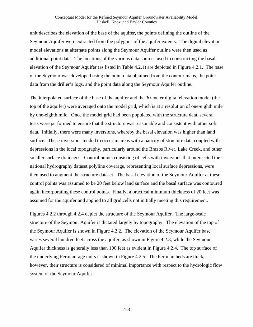
Conceptual Model for the Refined Seymour Aquifer Groundwater Availability Model: Haskell, Knox, and Baylor Counties
4-8
unit describes the elevation of the base of the aquifer, the points defining the outline of the
Seymour Aquifer were extracted from the polygons of the aquifer extents. The digital elevation
model elevations at alternate points along the Seymour Aquifer outline were then used as
additional point data. The locations of the various data sources used in constructing the basal
elevation of the Seymour Aquifer (as listed in Table 4.2.1) are depicted in Figure 4.2.1. The base
of the Seymour was developed using the point data obtained from the contour maps, the point
data from the driller’s logs, and the point data along the Seymour Aquifer outline.
The interpolated surface of the base of the aquifer and the 30-meter digital elevation model (the
top of the aquifer) were averaged onto the model grid, which is at a resolution of one-eighth mile
by one-eighth mile. Once the model grid had been populated with the structure data, several
tests were performed to ensure that the structure was reasonable and consistent with other soft
data. Initially, there were many inversions, whereby the basal elevation was higher than land
surface. These inversions tended to occur in areas with a paucity of structure data coupled with
depressions in the local topography, particularly around the Brazos River, Lake Creek, and other
smaller surface drainages. Control points consisting of cells with inversions that intersected the
national hydrography dataset polyline coverage, representing local surface depressions, were
then used to augment the structure dataset. The basal elevation of the Seymour Aquifer at these
control points was assumed to be 20 feet below land surface and the basal surface was contoured
again incorporating these control points. Finally, a practical minimum thickness of 20 feet was
assumed for the aquifer and applied to all grid cells not initially meeting this requirement.
Figures 4.2.2 through 4.2.4 depict the structure of the Seymour Aquifer. The large-scale
structure of the Seymour Aquifer is dictated largely by topography. The elevation of the top of
the Seymour Aquifer is shown in Figure 4.2.2. The elevation of the Seymour Aquifer base
varies several hundred feet across the aquifer, as shown in Figure 4.2.3, while the Seymour
Aquifer thickness is generally less than 100 feet as evident in Figure 4.2.4. The top surface of
the underlying Permian-age units is shown in Figure 4.2.5. The Permian beds are thick,
however, their structure is considered of minimal importance with respect to the hydrologic flow
system of the Seymour Aquifer.
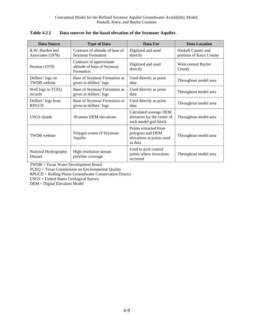
Conceptual Model for the Refined Seymour Aquifer Groundwater Availability Model: Haskell, Knox, and Baylor Counties
4-9
Table 4.2.1 Data sources for the basal elevation of the Seymour Aquifer.
Data Source Type of Data Data Use Data Location
R.W. Harden and Associates (1978)
Contours of altitude of base of Seymour Formation
Digitized and used directly
Haskell County and portions of Knox County
Preston (1978) Contours of approximate altitude of base of Seymour Formation
Digitized and used directly
West-central Baylor County
Drillers’ logs on TWDB website
Base of Seymour Formation as given in drillers’ logs
Used directly as point data
Throughout model area
Well logs in TCEQ records
Base of Seymour Formation as given in drillers’ logs
Used directly as point data
Throughout model area
Drillers’ logs from RPGCD
Base of Seymour Formation as given in drillers’ logs
Used directly as point data
Throughout model area
USGS Quads 30-meter DEM elevations Calculated average DEM elevation for the center of each model grid block
Throughout model area
TWDB website Polygon extent of Seymour Aquifer
Points extracted from polygons and DEM elevations at points used as data
Throughout model area
National Hydrography Dataset
High resolution stream polyline coverage
Used to pick control points where inversions occurred
Throughout model area
TWDB = Texas Water Development Board TCEQ = Texas Commission on Environmental Quality RPGCD = Rolling Plains Groundwater Conservation District USGS = United States Geological Survey DEM = Digital Elevation Model
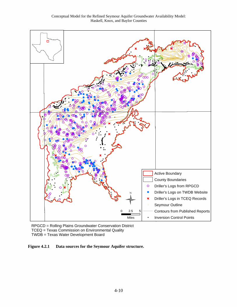
Conceptual Model for the Refined Seymour Aquifer Groundwater Availability Model: Haskell, Knox, and Baylor Counties
4-10
!
!
! !! ! !
!
!!
! !!
!
! !!
! !!! ! ! !!!! ! !! ! ! !! ! ! ! !! !! ! ! !! !! ! ! !!!! ! ! ! !!!!! !! !!! ! !! ! ! ! !!!!!!!!!!!!!!!!! !! ! !!!! !! ! ! !!! !! ! !! !! !!!!!! ! !!! !! ! !! !!! ! ! !! !!! !!! ! ! !! !! !!!!!! ! !! !!! ! ! ! !! ! ! ! ! !! ! ! !! ! !!!!! !!!! !! !!! !!! !! ! ! !! !!! ! ! ! !!! ! !! !! ! ! !! ! !!!! ! ! !!! ! ! ! ! !! ! ! ! !! ! ! !!! !!!!!! ! ! !!! !! ! !! ! !!!! !!! ! ! ! ! !!! ! !! !! ! ! !
! ! !!!!! !!
! !! !! ! ! !! !! !! !!! !! !! !! !!!! !!! !!!!!!! !!!!!! !!!!!!! !! !!!
!
!! !!!!
! !!!!! ! !!! !! ! !! ! !! ! !! ! !!! ! !! !! !! !! !
! ! ! !!!!!!!!!! !!!!!!!!!!
!!
!
!! !
!
!! !!! ! !
! !!!
! !!
!!
! !! !
!! !
!!! !!!! !
!! ! !!!! !!!!!! !!!!!!!!! !! !!
!!! !
! !
!
!
!!
!
!! !
!!! !
! ! !!! !! !! ! !
! ! !! ! !!
!! !
!!
! !
!!
! !
!! !
!!
0 2.5 5
Miles
Active Boundary
County Boundaries
Driller's Logs from RPGCD
Driller's Logs on TWDB Website
Driller's Logs in TCEQ Records
Seymour Outline
Contours from Published Reports
! Inversion Control Points
RPGCD = Rolling Plains Groundwater Conservation District TCEQ = Texas Commission on Environmental Quality TWDB = Texas Water Development Board
Figure 4.2.1 Data sources for the Seymour Aquifer structure.

Conceptual Model for the Refined Seymour Aquifer Groundwater Availability Model: Haskell, Knox, and Baylor Counties
4-11
King
Knox
Baylor
Haskell
Stonewall
Throckmorton
0 2.5 5
Miles
Active Boundary
County Boundaries
Elevation of Seymour Top
(feet)
1200 - 1250
1250 - 1300
1300 - 1350
1350 - 1400
1400 - 1450
1450 - 1500
1500 - 1550
1550 - 1600
1600 - 1650
1650 - 1700
1700 - 1750
Figure 4.2.2 Structure map of the top of the Seymour Aquifer.
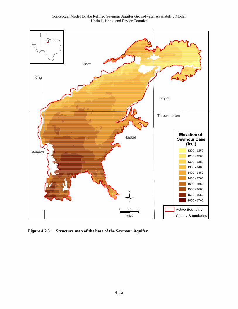
Conceptual Model for the Refined Seymour Aquifer Groundwater Availability Model: Haskell, Knox, and Baylor Counties
4-12
King
Knox
Baylor
Haskell
Stonewall
Throckmorton
0 2.5 5
Miles
Active Boundary
County Boundaries
Elevation of Seymour Base
(feet)
1200 - 1250
1250 - 1300
1300 - 1350
1350 - 1400
1400 - 1450
1450 - 1500
1500 - 1550
1550 - 1600
1600 - 1650
1650 - 1700
Figure 4.2.3 Structure map of the base of the Seymour Aquifer.

Conceptual Model for the Refined Seymour Aquifer Groundwater Availability Model: Haskell, Knox, and Baylor Counties
4-13
King
Knox
Baylor
Haskell
Stonewall
Throckmorton
0 2.5 5
Miles
Active Boundary
County Boundaries
SeymourIsopach
(feet)
20 - 30
30 - 40
40 - 50
50 - 60
60 - 70
70 - 80
80 - 90
90 - 100
100 - 110
Figure 4.2.4 Isopach map of the Seymour Aquifer.
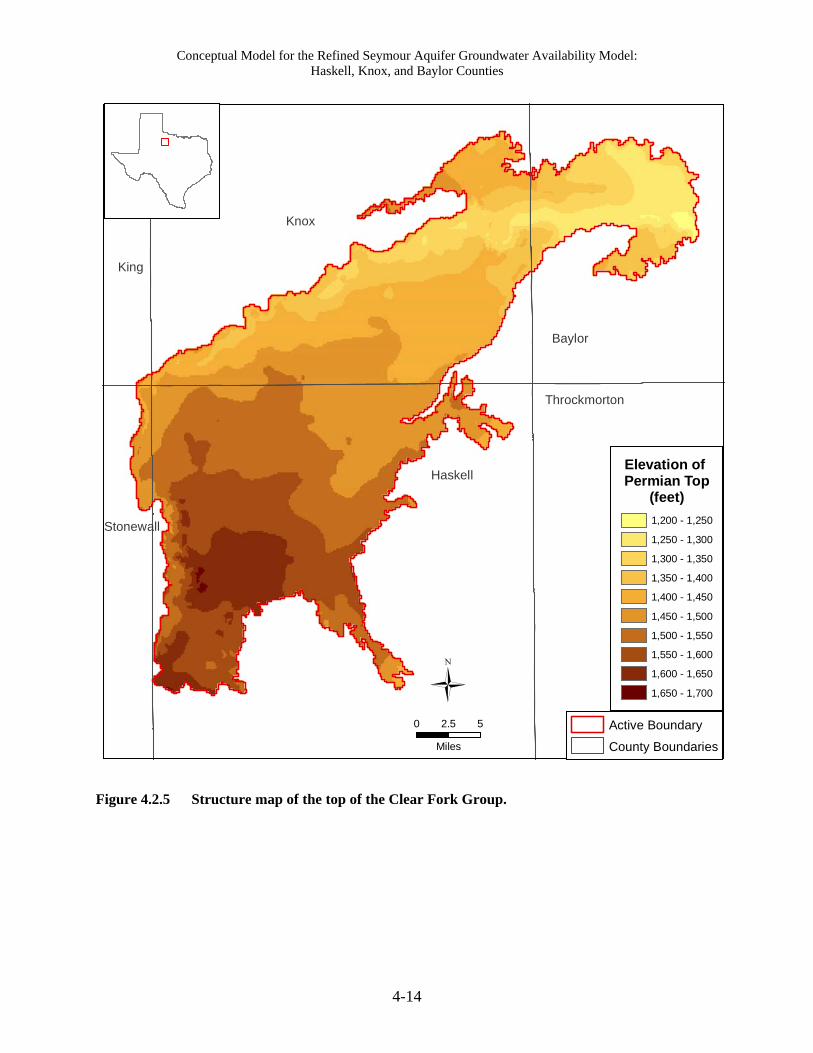
Conceptual Model for the Refined Seymour Aquifer Groundwater Availability Model: Haskell, Knox, and Baylor Counties
4-14
King
Knox
Baylor
Haskell
Stonewall
Throckmorton
0 2.5 5
Miles
Active Boundary
County Boundaries
Elevation of Permian Top
(feet)
1,200 - 1,250
1,250 - 1,300
1,300 - 1,350
1,350 - 1,400
1,400 - 1,450
1,450 - 1,500
1,500 - 1,550
1,550 - 1,600
1,600 - 1,650
1,650 - 1,700
Figure 4.2.5 Structure map of the top of the Clear Fork Group.
Conceptual Model for the Refined Seymour Aquifer Groundwater Availability Model: Haskell, Knox, and Baylor Counties
4-15
4.3 Water Levels and Regional Groundwater Flow
A literature search was conducted to understand regional groundwater flow and historical
conditions in the Seymour Aquifer. The primary sources used to obtain information regarding
groundwater flow in the Seymour Aquifer were the report on groundwater resources in Haskell
and Knox counties by Ogilbee and Osborne (1962), the report on the occurrence and quality of
groundwater in Baylor County by Preston (1978), the report on the Seymour Aquifer in Haskell
and Knox counties by R.W. Harden and Associates (1978), the survey of public water supplies in
central and north-central Texas by Sundstrom and others (1949), and the report on the geology
and groundwater of the Wichita Region in north-central Texas by Gordon (1913). In addition,
water-level data provided on the TWDB website (TWDB, 2008c) and the United States
Geological Survey website (United States Geological Survey, 2009a) were used to (1) develop
water-level elevations for steady-state conditions, the start time for the transient model
calibration period (January 1980), the middle time for the transient model calibration period
(January 1990), and the end of the transient model calibration period (December 1997); (2)
investigate transient water-level conditions; and (3) investigate cross-formational flow. Note that
almost all of the water-level data on the United States Geological Survey website (United States
Geological Survey, 2009a) are contained in the data from the TWDB website (TWDB, 2008c).
Water-level data for the Seymour Aquifer from the TWDB website (TWDB, 2008c), the United
States Geological Survey website (United States Geological Survey, 2009a), and Sundstrom and
others (1949) consist of 5,993 water-level measurements taken in 1,503 wells. The locations of
wells with water-level data are shown in Figure 4.3.1. Five hundred and sixty eight, 630, and
305 Seymour Aquifer wells are located in Haskell, Knox, and Baylor counties, respectively.
Only six wells and a total of 29 water-level measurements are available for the portion of the pod
in Stonewall County. For this discussion, those wells and measurements have been combined
with those for Haskell County. The number of water-level measurements by county is 3,124 for
Haskell County, 2,092 for Knox County, and 777 for Baylor County. The frequency of water-
level measurements with time is shown in Figure 4.3.2. The largest number of measurements
was taken in 1956 in Haskell and Knox counties and in 1969 in Baylor County. The low number
of measurements prior to 1956 is likely due to there being fewer wells completed into the
Conceptual Model for the Refined Seymour Aquifer Groundwater Availability Model: Haskell, Knox, and Baylor Counties
4-16
Seymour Aquifer prior to that time. Note that the number of water-level measurements for the
time period corresponding to the beginning (1980), middle (1990), and end (1997) of model
calibration is low.
4.3.1 Historical Water-Level Fluctuations in the Seymour Aquifer
Land use over the Haskell-Knox-Baylor pod of the Seymour Aquifer changed significantly
between about 1880 and 1930 as summarized in Section 2.3. Those changes appear to have
impacted recharge to and natural discharge from the Seymour Aquifer, which caused significant
fluctuations in water levels in portions of the aquifer. The fact that large changes in water levels
resulted from changes in recharge and natural discharge is likely due to the thin nature of the
aquifer and the relatively short time required for water to infiltrate through the unsaturated zone
and reach the water table. This section contains a summary of historical water levels in the
Seymour Aquifer prior to significant pumping, which began in the 1950s. A description of land
use changes and how they affected the Seymour Aquifer can be found in Section 5.0.
Groundwater in the Seymour Aquifer was under steady-state conditions, where recharge and
natural discharge were balanced resulting in no net change in storage, prior to about 1880. Water
levels in the Seymour Aquifer under this steady-state condition are unknown. However, it is
likely that the aquifer had some saturated thickness over most of its area because of the sandy
nature of the surface soil and the fact that the aquifer is shallow. The presence of buffalo bones
and Indian artifacts at several springs flowing from the Seymour Aquifer (see Section 4.5.2)
supports this theory.
The steady-state condition of the Seymour Aquifer was disrupted by anthropogenic activities
related to the introduction of livestock and agriculture to the area. Overgrazing by domestic
livestock and the resultant increase in number and areal distribution of honey mesquite may have
caused an increase in natural aquifer discharge due to an increase in water-table
evapotranspiration by mesquite tap roots. In addition, degradation of the surface soil caused by
overgrazing probably resulted in some decrease in aquifer recharge due to decreased infiltration
of precipitation. Sherrill (1965) reports that Haskell County experienced two years of major
drought (1886 and 1896) and several years of light rainfall (1890 through 1893, 1901, 1904, and
1910) between 1880 and 1910. These periods of reduced precipitation would have also

Conceptual Model for the Refined Seymour Aquifer Groundwater Availability Model: Haskell, Knox, and Baylor Counties
4-17
contributed to decreased aquifer recharge. It is possible that water levels in portions of the
Seymour Aquifer declined as a result of increased natural aquifer discharge and decreased
recharge, which may have caused drying out of the aquifer in areas where it is thin and the
density of phreatophytes was high and/or located in areas where recharge was reduced.
Historical accounts by Gordon (1913), based on field work conducted in 1906 and 1907, indicate
that portions of the Seymour Aquifer were dry in the early 1900s. Gordon (1913) reports that
groundwater was not found throughout the Seymour Formation in Haskell and Knox counties.
He does not mention specific locations in Knox County where groundwater was found in the
Seymour Formation, but does provide some detail for Haskell County. He states that
groundwater was found in the basal gravel in the Seymour Formation in the city of Haskell but
that "On approaching the Double Mountain Fork, … these beds appear to be bereft of water and
the wells extend some distance into the red clays (Permian) before striking water…" However,
he also states that "many wells in the western part of Haskell County derive their supplies from
the Seymour formation at depths of 40 to 50 feet". Based on the driller's record given in Gordon
(1913) for two wells in the city of Rule, one well 10 miles northwest of the city, and one well
about 12 miles southwest of the city, water was not found in these wells until they penetrated the
Permian-age sediments. Gordon (1913) reports that water was found in the Seymour Formation
at depths of about 15 to 45 feet in western Baylor County, suggesting that this portion of the
aquifer received sufficient recharge to sustain some saturated thickness. Preston (1978) states
that "oldtimers" in Baylor County report that "where the Seymour Formation is well
developed…there were only small amounts of water available from the Seymour 40 or 50 years
ago".
Farming in Haskell, Knox, and Baylor counties boomed between about 1900 and 1910 and about
1920 and 1930 (Texas State Historical Association, 2008), which brought with it land use
changes. Improving the surface soil through clearing, plowing, and terracing the land appears to
have increased recharge to the Seymour Aquifer. It is also likely that clearing honey mesquite
and the native grasses and planting crops reduced natural discharge via evapotranspiration.
These changes in recharge and natural discharge could have caused the water-level rises
experienced in some areas of the aquifer due to aquifer recharge exceeding natural aquifer
discharge. Bandy (1934), as reported in Ogilbee and Osborne (1962) and R.W. Harden and
Associates (1978), provides information on significant water-level rises in portions the Seymour

Conceptual Model for the Refined Seymour Aquifer Groundwater Availability Model: Haskell, Knox, and Baylor Counties
4-18
Aquifer between about 1909 and 1934. He interviewed residents and inventoried wells in
northwestern Haskell County in 1934 to investigate reported rises in water levels in the aquifer.
Some of the information reported by Bandy (1934) based on those interviews includes:
the depth to water in the city of Rochester well was 45 feet below ground surface in 1926
and 35 feet below ground surface in 1934 with 4 feet of the water-level rise occurring in
the last two years (1932 to 1934),
water in a well located 5 miles west of the city of Rochester was 70 to 75 feet below
ground surface and hard and gip 25 years ago (about 1909) and 45 feet below ground
surface and soft and fresh in 1934,
water in a well located 8 miles west of the city of Rochester was 74 feet below ground
surface when it was dug (date not given) and 13 feet below ground surface in 1934,
in a well located near the old city of Judd, the depth to water was 10 feet when it was dug
(date not given) and water was running out of the well in 1934,
in a well located 1 mile west of Rochester, the depth to water was 75 feet below land
surface when it was dug (date not given) and was 45 feet below ground surface in 1934,
and
water has risen to the top of several wells resulting in the development of marsh land.
Bandy (1934) also stated that:
"…the rise of ground water in this area is no myth, but a fact, that the rise has been about
a foot per year with some little acceleration during the last few years, and the water has changed
from hard, gip and salt water to soft, fresh water. …. This has been very beneficial to this county
until recent years; for fresh water had been very hard to obtain, but in 1928 numerous small spots
of water-logged land began to appear here and there, the following year changing to a salt marsh
which was wholly non-productive. These spots have increased in size year by year until at this
date there are some of from five to one hundred twenty acres; they would aggregate probably
200 acres at the present time."

Conceptual Model for the Refined Seymour Aquifer Groundwater Availability Model: Haskell, Knox, and Baylor Counties
4-19
R.W. Harden and Associates (1978) tried to determine the locations of the wells in Bandy's
investigation, but could not. They did conclude that his records indicated that the water-level
rises were observed in the vicinity of the cities of Rochester and O'Brien. R.W. Harden and
Associates (1978) summarized the water-level rises reported by Bandy (1934) in a figure, which
is reproduced in Figure 4.3.3. This figure indicates rises of up to about 69 feet over about a
20-year period.
Additional information regarding the rise in water levels in the Seymour Aquifer is found in
Sundstrom and others (1949), who inventoried public water supplies in the central and north-
central Texas. They report that:
a municipal well for the city of Rochester had a depth to water of 46 feet below ground
surface when dug in 1926 and 15 feet below ground surface on March 24, 1944,
a municipal well for the city of Rule had a depth to water of 28 feet below ground surface
when dug in 1923 and 32 feet below ground surface on March 20, 1944; recall that
Gordon (1913) stated that groundwater was not found in the Seymour Formation in
1906/1907 in the vicinity of the city of Rule, and
a municipal well for the city of Goree, dug in 1925, had a depth to water of 28 feet below
ground surface in 1938 and 21.7 feet below ground surface on March 22, 1944.
The information reported in Bandy (1934), Sundstrom and others (1949), and Preston (1978)
support the theory that water levels in the Seymour Aquifer increased substantially in some areas
after the early 1900s. These water-level rises appear to be the result of increased aquifer
recharge and decreased natural aquifer discharge due to land use changes related to agricultural
development in the area. Ogilbee and Osborne (1962) state that "The period of rising water
levels corresponds with the period of rapid agricultural development and also approximately
corresponds with a period of above normal precipitation. Both conditions may be factors in
causing the rise in water levels."
How water levels in the Seymour Aquifer changed between 1934 and the early 1950s is
unknown. Water-level measurements are available for six wells in 1944 and then again in 1951.
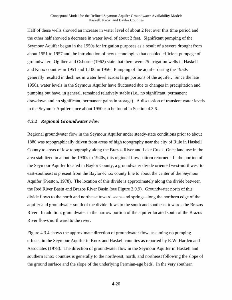
Conceptual Model for the Refined Seymour Aquifer Groundwater Availability Model: Haskell, Knox, and Baylor Counties
4-20
Half of these wells showed an increase in water level of about 2 feet over this time period and
the other half showed a decrease in water level of about 2 feet. Significant pumping of the
Seymour Aquifer began in the 1950s for irrigation purposes as a result of a severe drought from
about 1951 to 1957 and the introduction of new technologies that enabled efficient pumpage of
groundwater. Ogilbee and Osborne (1962) state that there were 25 irrigation wells in Haskell
and Knox counties in 1951 and 1,100 in 1956. Pumping of the aquifer during the 1950s
generally resulted in declines in water level across large portions of the aquifer. Since the late
1950s, water levels in the Seymour Aquifer have fluctuated due to changes in precipitation and
pumping but have, in general, remained relatively stable (i.e., no significant, permanent
drawdown and no significant, permanent gains in storage). A discussion of transient water levels
in the Seymour Aquifer since about 1950 can be found in Section 4.3.6.
4.3.2 Regional Groundwater Flow
Regional groundwater flow in the Seymour Aquifer under steady-state conditions prior to about
1880 was topographically driven from areas of high topography near the city of Rule in Haskell
County to areas of low topography along the Brazos River and Lake Creek. Once land use in the
area stabilized in about the 1930s to 1940s, this regional flow pattern returned. In the portion of
the Seymour Aquifer located in Baylor County, a groundwater divide oriented west-northwest to
east-southeast is present from the Baylor-Knox county line to about the center of the Seymour
Aquifer (Preston, 1978). The location of this divide is approximately along the divide between
the Red River Basin and Brazos River Basin (see Figure 2.0.9). Groundwater north of this
divide flows to the north and northeast toward seeps and springs along the northern edge of the
aquifer and groundwater south of the divide flows to the south and southeast towards the Brazos
River. In addition, groundwater in the narrow portion of the aquifer located south of the Brazos
River flows northward to the river.
Figure 4.3.4 shows the approximate direction of groundwater flow, assuming no pumping
effects, in the Seymour Aquifer in Knox and Haskell counties as reported by R.W. Harden and
Associates (1978). The direction of groundwater flow in the Seymour Aquifer in Haskell and
southern Knox counties is generally to the northwest, north, and northeast following the slope of
the ground surface and the slope of the underlying Permian-age beds. In the very southern

Conceptual Model for the Refined Seymour Aquifer Groundwater Availability Model: Haskell, Knox, and Baylor Counties
4-21
portion of the aquifer in Haskell County, groundwater flow is generally to the east and southeast
with some flow also to the southwest.
4.3.3 Steady-State Conditions
Steady-state conditions for typical aquifers coincide with the time period prior to significant
pumpage. For the Seymour Aquifer, however, steady-state conditions were disrupted by land
use changes beginning in about 1880, many years prior to the advent of significant pumping in
the 1950s. Brune (2002) reports that buffalo bones and Indian artifacts were found at several
springs flowing from the Seymour Aquifer. This is evidence that the aquifer had some saturated
thickness under steady-state conditions. Water-level data are not available prior to the late
1800s; therefore, no water-level targets for the steady-state period are available. However, the
elevations of the springs flowing from the aquifer during this time provide a minimum elevation
for water levels. The exact location is available for only a few of these historical springs (see
Section 4.5.2). The elevations of the historical springs with known locations are posted on
Figure 4.3.5. No attempt was made to contour these elevations because the data are insufficient
to appropriately represent the variability in the water table due to the variability in the
topography. The elevations on Figure 4.3.5 provide a minimum elevation for the Seymour
Aquifer under steady-state conditions.
Estimated steady-state water-level elevations for the Permian-age formations are shown in
Figure 4.3.6. Due to the sparse data for the Permian formations in the model area, data from
several counties surrounding the model area, as shown in Figure 4.3.7, were included in
developing these contours. The steady-state water-level elevations for the Permian-age
formations were taken as the first water-level measurements for wells with relatively stable water
levels throughout time and with depths to water less than 200 feet. This latter criterion was used
because only the upper portion of the Permian-age formations may affect the hydrologic flow
system of the Seymour Aquifer.
4.3.4 Water-Level Elevations for Transient Model Calibration
Transient model calibration considers the time period from January 1, 1980 to December 31,
1997. Water-level data obtained from the TWDB website (TWDB, 2008c) and the United States

Conceptual Model for the Refined Seymour Aquifer Groundwater Availability Model: Haskell, Knox, and Baylor Counties
4-22
Geological Survey (United States Geological Survey, 2009a) were used to develop water-level
elevations for the Seymour Aquifer and the underlying Clear Fork Group for the start of the
transient model calibration (January 1980), the middle of the transient model calibration
(January 1990), and the end of the transient model calibration (December 1997). These water-
level elevations were used to aid in assessing the transient model's ability to represent observed
conditions.
Water-level data are not available at regular time intervals in every well. Therefore, the
coverage of water-level data for a particular month or even a year is very sparse. Since the
amount of water-level data available for the times of interest were not sufficient to develop
contours, data for the year of interest and for two years prior to and two years after the year of
interest were used. If a well had only one water-level measurement during that time, that
measurement was used. If a well had several water-level measurements during that time, the
average of the water levels was used.
Because the Seymour Aquifer is shallow, thin, and responds quickly to recharge, seasonal
changes in precipitation and pumping are readily observed in water levels in most areas of the
aquifer as discussed in Section 4.3.6. In order to compare water levels in the aquifer at the
beginning, middle, and end of the transient model calibration period, only water levels measured
during the winter months (November through March), when water levels in the aquifer are least
effected by irrigation pumping and precipitation, were used to create contours of water-level
elevations for these three time periods. In order to meaningfully evaluate the model's ability to
reproduce observed conditions, water-level elevations predicted by the model during the winter
months was compared to these contours.
Figures 4.3.8, 4.3.9, and 4.3.10 show water-level elevation contours in the Seymour Aquifer at
the beginning, middle, and end of the model calibration period, respectively. These contours
show that the water level was highest near the city of Rule and decreased in all directions out
from the maximum for all three time periods. Table 4.3.1 presents the water-level elevations for
wells having data for at least two out of the three years of interest for the transient model
calibration. This table also provides an indication of the trend in the water level, the magnitude
of observed increases and decreases in water level, and the overall change in water level between

Conceptual Model for the Refined Seymour Aquifer Groundwater Availability Model: Haskell, Knox, and Baylor Counties
4-23
1980 and 1997, with the exception of well 21-33-940 where the overall change is for the period
between 1990 and 1997. The information in Table 4.3.1 is also plotted on Figure 4.3.11. The
site numbers used to identify wells on this figure are included in Table 4.3.1. An overall increase
of more than 5 feet was observed at site 1 in Baylor County, site 23 in Knox County, and sites 13
and 17 through 19 in Haskell County. An overall decrease of more than 5 feet was observed
only at site 12 in Haskell County. In general, overall increases were observed in Baylor, Knox,
and the southern portion of the pod in Haskell County and overall decreases were observed in the
central portion of the pod in Haskell County.
Figures 4.3.12, 4.3.13, and 4.3.14 show water-level elevation contours for the Permian-age
formations in the model area at the start, middle, and end of the transient model calibration
period, respectively. Due to the sparse data for the Permian-age formations within the model
area, data from several counties surrounding the model area (see Figure 4.3.7) were included in
developing these contours. These figures indicate that flow in the Permian-age formations is
from topographic highs on the western side of the model area to topographic lows on the eastern
side. Very little change in water levels occurred in the Permian-age formations between 1980
and 1997. A comparison of these contours to the contours of steady-state water-level elevations
in Figure 4.3.6 indicate that water levels in the Permian-age formations were about 25 feet higher
under steady-state conditions.
4.3.5 Cross-Formational Flow
An exercise was conducted to investigate cross-formational flow between the Seymour Aquifer
and the underlying Clear Fork Group. Vertical flow within the Seymour Aquifer itself was not
evaluated due to the thin nature of the aquifer. At three locations in the model area, wells
completed separately to the Seymour Aquifer and the Clear Fork Group share a similar surface
location. The comparison of water-level elevations in those wells is shown in Figure 4.3.15 and
Table 4.3.2.
For the location in Haskell County, the water-level elevations in the wells completed into the
Seymour Aquifer are higher than those in the wells completed into the Clear Fork Group. For all
the wells at this location, the water level was measured in January, March, or October, with the
exception of one measurement in May 1956 for well 21-49-902 completed into the Clear Fork
Conceptual Model for the Refined Seymour Aquifer Groundwater Availability Model: Haskell, Knox, and Baylor Counties
4-24
Group. In this area, the water-level elevations in the Seymour Aquifer are higher than those in
the Clear Fork Group. This could indicate a potential for flow from the Seymour Aquifer to the
Clear Fork Group. However, the land surface elevations for the wells completed into the
Seymour Aquifer are higher than those for the wells completed into the Clear Fork Group. This
difference in land surface elevation could explain the difference in water-level elevations. If a
downward gradient does exist between the two formations, the amount of flow is most likely
small due to the low permeability of the sediments making up the Clear Fork Group. This
conclusion is supported by the difference in the chemical quality of the water in the Seymour
Aquifer and the Clear Fork Group (Ogilbee and Osborne, 1962).
For the western-most cluster in Baylor County, the water-level elevation in the well completed
into the Clear Fork Group is lower than that in one nearby Seymour Aquifer well and higher than
that in three other nearby Seymour Aquifer wells. The wide range in water-level elevations for
wells completed into the Seymour Aquifer at this location likely reflects the range in water levels
in the aquifer due to seasonal changes (see Section 4.3.6) and/or the range in land surface
elevation. For the wells completed into the Seymour Aquifer at this location, the water level was
measured in April or June in the three wells with a water-level elevation below the water-level
elevation in the Clear Fork Group (wells 21-29-310, 21-29-307, and 21-29-302) and was
measured in January and February in the one well (well 21-29-306) with a water-level elevation
above the water-level elevation in the Clear Fork Group. In addition, the land surface elevation
at the well completed into the Clear Fork Group is 19 feet below that for the Seymour Aquifer
well with the higher water-level elevation (well 21-29-306) and is 21 to 33 feet above that for the
three Seymour Aquifer wells with the lower water-level elevation (wells 21-29-310, 21-29-307,
and 21-29-302). The fact that the water-level elevation in the Clear Fork Group at this location
falls between the water-level elevations in the Seymour Aquifer could be a function of seasonal
fluctuations in water levels in the Seymour Aquifer and/or a function of the difference in the
ground surface elevation at the wells. Therefore, no clear conclusion can be made regarding the
direction of the gradient between the Seymour Aquifer and the Clear Fork Group at this location.
For the eastern-most cluster in Baylor County, the water-level elevation in the well completed
into the Clear Fork Group is about 10 feet lower than the water-level elevation in three nearby
wells completed into the Seymour Aquifer (wells 21-30-110, 21-30-118, and 21-30-121) and

Conceptual Model for the Refined Seymour Aquifer Groundwater Availability Model: Haskell, Knox, and Baylor Counties
4-25
about 50 feet higher than the water-level elevation in two other nearby wells completed into the
Seymour Aquifer (wells 21-30-109 and 21-30-124). At this location, the large range in water-
level elevations in the Seymour Aquifer appears to be due to the large difference in ground
surface elevation at the wells rather than seasonal fluctuations in water levels. For the two
Seymour Aquifer wells with water-level elevations below that in the Permian well, the ground
surface elevation is about 40 feet below the ground surface elevation of the Clear Fork Group
well. For the three Seymour Aquifer wells with water-level elevations above that in the Clear
Fork Group well, the ground surface elevation is 16 feet above the ground surface elevation of
the Clear Fork Group well. The fact that the water-level elevation in the Clear Fork Group at
this location falls between the water-level elevations in the Seymour Aquifer could be a function
of the differences in ground surface elevation at the wells. Therefore, no clear conclusion can be
made regarding the direction of the gradient between the Seymour Aquifer and Clear Fork Group
at this location.
All of the water-level data shown in the comparisons in Figure 4.3.15 are for a time prior to the
time period for the transient model calibration. A comparison of the water-level elevation
contours for the start, middle, and end of the transient model calibration period between the
Seymour Aquifer (Figures 4.3.8 through 4.3.10) and the Permian-age formations (Figures 4.3.12
through 4.3.14) indicate higher water levels in the Seymour Aquifer than in the Permian-age
formations for all three times in Baylor County and in Haskell County in the vicinity of the city
of Rule where the maximum water levels in the Seymour Aquifer are observed. The water level
in the Permian-age formations is higher than in the Seymour Aquifer along the western edge of
the pod in Haskell and Knox counties. Although the water level in the Seymour Aquifer is
higher than in the Permian-age formations in some areas, low flow rates from the Seymour
Aquifer to the underlying Permian-age formations are expected due to the low permeability of
the predominantly shale Permian-age sediments. The difference in the chemical quality of the
groundwater in the Seymour Aquifer and Permian-age formations also suggests little flow
between the two, however, the chemical quality in the Permian-age formations may be more
indicative of long-term, pre-development conditions than of more recent (since 1910) conditions
where recharge is conceptualized to have increased. The low cross-formational flow rates, when
aggregated over the entire aquifer, may amount to a significant portion of the Seymour Aquifer
water budget.

Conceptual Model for the Refined Seymour Aquifer Groundwater Availability Model: Haskell, Knox, and Baylor Counties
4-26
4.3.6 Transient Water Levels
Transient water-level data are used in calibration of the transient model. Figure 4.3.16 shows the
locations of the 135 wells for which transient water-level data, defined as five or more water-
level measurements, are available for the Seymour Aquifer based on data found on the TWDB
and United States Geological Survey websites (TWDB, 2008c and United States Geological
Survey, 2009a, respectively) and in Sundstrom and others (1949). Table 4.3.3 summarizes the
wells with transient water-level data, the year of the first and last water-level measurement, and
the total number of water-level measurements. For a little over half of these wells, ten or fewer
measurements are available over a period of only a year or two. Therefore, data for those wells
give little information on long-term trends within the aquifer. Notice that no water-level data
during the time period when the aquifer was filling up (about 1910 to 1940) are available for any
of these wells. Note that although the wells from Bandy (1934) do have data during this time
period, their locations and state well numbers, if any, are not known.
Figures 4.3.17 through 4.3.23 contain hydrograph plots of the transient water-level data at
selected wells. Most of these hydrographs are plotted with a 50-foot elevation difference on the
y-axis. In some cases, the difference in water-level elevations was greater than 50 feet and the
y-axis was expanded. In all cases, the interval between grid lines on the y-axis is 5 feet. The
base of the well is shown on all of the hydrograph plots. The base of the well is assumed to
represent the base of the Seymour Aquifer because most wells were drilled only into the top few
inches of the underlying Clear Fork Group. Adding the base of the well to the hydrograph plots
provides a means to evaluate the saturated thickness of the aquifer with time.
Water-level elevations for the five wells in Baylor County with the most comprehensive transient
data are shown in Figure 4.3.17. This figure shows that the water level has remained relatively
stable in one of the wells, has slightly increased in three of the wells, and has slightly decreased
in one of the wells. The magnitude of the observed increases ranges from less than 5 feet to
about 10 feet and the magnitude of the observed decrease is about 5 feet.
In Haskell County, long-term water-level data extending through the transient model calibration
period are available for 19 wells. The data for 13 of these wells shows a decrease in water level
from the start of the record in the 1950s to around 1960 or 1965 followed by an increase in water

Conceptual Model for the Refined Seymour Aquifer Groundwater Availability Model: Haskell, Knox, and Baylor Counties
4-27
level until about 1990 and then another decrease in water level, with the magnitude of the
decreases and increases ranging from about 10 to 30 feet. Transient data at several wells that
exhibit this trend in long-term water levels are shown in Figure 4.3.18. Although the water
levels in these wells show fairly large fluctuations relative to the saturated thickness of the
aquifer, they do not indicate an overall increase or decrease in water level in the aquifer. In
addition to the fluctuating trend observed in most wells in Haskell County, an increase in water
level is observed in five wells for which long-term data are available and a stable water-level
trend is observed in one well (Figure 4.3.19). The magnitude of the increases ranges from about
3 to 25 feet. The earliest water-level measurement in Haskell County was taken in 1926 in a city
of Rochester well (well 21-42-401). The transient data for this well (Figure 4.3.19) shows an
increase in water level of about 30 feet between 1926 and 1944. This increase reflects a portion
of the time period during which parts of the Seymour Aquifer were gaining water. After 1944,
the water level in this well had decreased about 10 feet by about 1965, increased about 20 feet by
about 1995, and then decreased until the last measurement in 1996. The transient data for this
well indicates that, although the water level in the well fluctuated after the Seymour Aquifer
gained water, it never decreased to the level observed in 1926.
In Knox County, long-term water-level data extending through the transient model calibration
period are available for 16 wells. The water levels in four of those wells show an overall
decrease since about 1950 (Figure 4.3.20). The magnitude of the decreases ranges from about
6 feet to about 20 feet. For all four wells, the water levels remained stable or even increased
slightly from about 1980 to 2000, even though the overall long-term trend was a decline in water
level. The water levels in five wells with long-term data in Knox County show an initial
decrease followed by an increase (Figure 4.3.21). The time at which the trend changed from
decreasing to increasing ranges from about 1965 to about 1990. The magnitude of the decreases
ranges from about 10 to 20 feet and the magnitude of the increases ranges from about 5 to
15 feet. The water levels in four of the wells with long-term water-level data in Knox County
show an overall increasing trend since about 1955 to about 1990 (Figure 4.3.22). For three of
these wells, the water levels slightly decreased between 1990 and the end of the record. The
magnitude of the increases ranges from about 8 to 15 feet and the magnitude of the decreases
ranges from about 5 to 8 feet. The water levels in another three of the wells with long-term data

Conceptual Model for the Refined Seymour Aquifer Groundwater Availability Model: Haskell, Knox, and Baylor Counties
4-28
in Knox County show an overall stable trend (Figure 4.3.23). Although the water level in these
wells fluctuated with time, the overall trend is stable.
Long-term water-level data sufficient to evaluate seasonal trends are available for three unused
wells located in Knox and Haskell counties (Figure 4.3.24). The water level was measured
several times monthly in well 21-36-103 located in Knox County between July 1975 and
November 1977 and in well 21-35-748 located in Haskell County between August 2002 and
February 2008. In well 21-42-409 located in Haskell County, the water level was measured
several times monthly between July 1975 and December 1982 and approximately monthly
between January 1983 and March 1986. The water-level data for well 21-36-103 in Knox
County indicates a consistent decline in water level of about 3 feet over the 2.5-year record with
no indication of seasonal fluctuations. The first 3 years of data for well 21-35-748 in Haskell
County clearly show seasonal fluctuations with the minimum water level observed in about
August and the maximum water level observed in about April. The difference in water level
between the summer and winter seasons ranged from about 2 to 5 feet. The remaining 2.5 years
of the water-level record for this well also shows a minimum water level in about August but
does not show the clear fluctuations observed in the first 3 years of the record. The water-level
data for well 21-42-409 in Haskell County show an overall decline in the water level between
July 1975 and about August 1980 followed by an overall increase in the water level to the end of
the record. Superimposed on this general trend for well 21-42-409 are shorter term fluctuations,
but those fluctuations do not appear to reflect a consistent seasonal trend. For example, the water
level is relatively higher in the June to August period and relatively lower in the December to
March period for several years (i.e., 1976-1977, 1981-1982, and 1985), which seems inconsistent
with higher pumping and lower precipitation in summer months relative to winter months. The
expected trend is a lower water level in the summer months when irrigation pumping is high and
precipitation is low, which is observed only in 1978 and 1980. The data from these three wells
suggests that the water level in the Seymour Aquifer in Haskell and Knox counties fluctuates
seasonally in some areas but not in other areas.
Water levels measured every few months between December 1968 and February 1970 are
available for 15 wells in Baylor County. The locations of those wells along with their water-
level data during this time period and primary use, as indicated on the TWDB website (TWDB,

Conceptual Model for the Refined Seymour Aquifer Groundwater Availability Model: Haskell, Knox, and Baylor Counties
4-29
2008c), are shown in Figure 4.3.25. Note that the y-axis is different for every plot shown on this
figure and ranges from 10 to 20 feet. For the majority of these wells, the lowest water level was
observed in the July to September months and the highest water level was observed in the winter
months. The difference in water level between the summer and winter seasons ranged from as
little as about 0.5 feet to as much as about 5 feet. For the remaining wells, no seasonal change in
water level was observed over this time period. Note that a seasonal change was observed in all
of the wells whose primary use is irrigation. Based on these data, it appears that water levels in
the portion of the Seymour Aquifer located in Baylor County are lower in the summer months
and higher in the winter months.

Conceptual Model for the Refined Seymour Aquifer Groundwater Availability Model: Haskell, Knox, and Baylor Counties
4-30
Table 4.3.1 Comparison of average 1980, 1990, and 1997 water-level elevations in the Seymour Aquifer.
State Well
Number County
Site Number1
Average 1980 Water-Level
Elevation (feet)
Average 1990 Water-Level
Elevation (feet)
Average 1997 Water-Level
Elevation (feet)
Trend2 Magnitude of Increase
(feet)
Magnitude of Decrease
(feet)
Overall Change (feet)3
21-22-802 Baylor 1 1283.79 1288.96 1290.43 increasing 6.65 6.65 21-30-202 Baylor 2 1279.32 1283.34 1281.60 increasing-decreasing 4.02 1.74 2.29 21-30-204 Baylor 3 1272.91 1274.26 1272.90 increasing-decreasing 1.34 1.36 -0.01 21-34-702 Haskell 4 1533.93 1537.61 increasing 3.67 3.67 21-34-902 Haskell 5 1522.34 1519.16 decreasing 3.18 -3.18 21-35-702 Haskell 6 1507.41 1508.61 increasing 1.20 1.20 21-35-801 Haskell 7 1491.73 1493.14 increasing 1.41 1.41 21-42-104 Haskell 8 1567.65 1564.66 decreasing 2.99 -2.99 21-42-201 Haskell 9 1540.89 1540.95 increasing 0.06 0.06 21-42-202 Haskell 10 1535.64 1530.98 decreasing 4.66 -4.66 21-42-502 Haskell 11 1553.89 1552.43 decreasing 1.46 -1.46 21-42-701 Haskell 12 1623.10 1615.58 decreasing 7.52 -7.52 21-49-211 Haskell 13 1605.78 1613.20 increasing 7.42 7.42 21-49-301 Haskell 14 1648.42 1652.38 increasing 3.96 3.96 21-49-601 Haskell 15 1649.66 1650.11 increasing 0.45 0.45 21-49-603 Haskell 16 1648.12 1650.01 increasing 1.89 1.89 21-50-401 Haskell 17 1637.81 1647.67 increasing 9.86 9.86 21-50-402 Haskell 18 1632.80 1638.13 increasing 5.33 5.33 21-50-506 Haskell 19 1625.41 1632.04 increasing 6.62 6.62 21-51-702 Haskell 20 1564.85 1566.33 increasing 1.48 1.48 21-51-710 Haskell 21 1572.96 1575.36 increasing 2.40 2.40 21-20-901 Knox 22 1407.80 1411.46 1410.64 increasing-decreasing 3.66 0.82 2.85 21-27-801 Knox 23 1419.73 1428.49 1427.17 increasing-decreasing 8.76 1.32 7.43 21-29-102 Knox 24 1403.24 1406.44 1406.41 increasing-decreasing 3.20 0.03 3.17 21-33-940 Knox 25 1479.51 1478.55 decreasing 0.96 -0.96 21-34-202 Knox 26 1434.11 1434.65 1437.80 increasing 3.69 3.69 21-34-402 Knox 27 1456.79 1459.47 1457.07 increasing-decreasing 2.68 2.39 0.28 21-34-501 Knox 28 1509.76 1514.93 1511.91 increasing-decreasing 5.17 3.02 2.15 21-34-601 Knox 29 1489.40 1491.83 1493.90 increasing 4.50 4.50
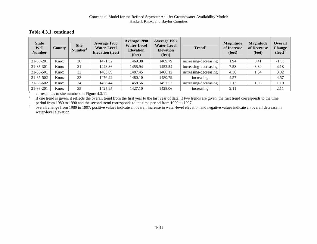
Conceptual Model for the Refined Seymour Aquifer Groundwater Availability Model: Haskell, Knox, and Baylor Counties
4-31
Table 4.3.1, continued
State Well
Number County
Site Number1
Average 1980 Water-Level
Elevation (feet)
Average 1990 Water-Level
Elevation (feet)
Average 1997 Water-Level
Elevation (feet)
Trend2 Magnitude of Increase
(feet)
Magnitude of Decrease
(feet)
Overall Change (feet)3
21-35-201 Knox 30 1471.32 1469.38 1469.79 increasing-decreasing 1.94 0.41 -1.53 21-35-301 Knox 31 1448.36 1455.94 1452.54 increasing-decreasing 7.58 3.39 4.18 21-35-501 Knox 32 1483.09 1487.45 1486.12 increasing-decreasing 4.36 1.34 3.02 21-35-502 Knox 33 1476.22 1480.10 1480.79 increasing 4.57 4.57 21-35-602 Knox 34 1456.44 1458.56 1457.53 increasing-decreasing 2.13 1.03 1.10 21-36-201 Knox 35 1425.95 1427.10 1428.06 increasing 2.11 2.11
1 corresponds to site numbers in Figure 4.3.11 2 if one trend is given, it reflects the overall trend from the first year to the last year of data; if two trends are given, the first trend corresponds to the time
period from 1980 to 1990 and the second trend corresponds to the time period from 1990 to 1997 3 overall change from 1980 to 1997; positive values indicate an overall increase in water-level elevation and negative values indicate an overall decrease in
water-level elevation

Conceptual Model for the Refined Seymour Aquifer Groundwater Availability Model: Haskell, Knox, and Baylor Counties
4-32
Table 4.3.2 Summary of data used to compare water-level elevations in the Seymour Aquifer and the underlying Clear Fork Group.
State Well Number
County Unit Date of
Water-Level Measurement
Elevation of Land
Surface Datum (feet)
Depth to Water (feet)1
Water-Level Elevation
(feet)2
Haskell County 21-49-907 Haskell Seymour Aquifer 3/21/1944 1683 -15.4 1667.6 21-49-907 Haskell Seymour Aquifer 1/6/1977 1683 -26.7 1656.3 21-49-906 Haskell Seymour Aquifer 1/6/1977 1690 -30.7 1659.3 21-49-606 Haskell Seymour Aquifer 1/6/1977 1686 -29.1 1656.9 21-49-903 Haskell Seymour Aquifer 3/21/1944 1686 -28.6 1657.4 21-49-903 Haskell Seymour Aquifer 10/18/1956 1686 -37.4 1648.6 21-49-903 Haskell Seymour Aquifer 1/6/1977 1686 -27.6 1658.4 21-49-901 Haskell Clear Fork Group 10/17/1956 1662 -32.6 1629.4 21-49-901 Haskell Clear Fork Group 1/6/1977 1662 -20.7 1641.3 21-49-901 Haskell Clear Fork Group 1/6/1977 1662 -20.7 1641.3 21-49-902 Haskell Clear Fork Group 5/25/1956 1636 -18.2 1617.8 21-49-902 Haskell Clear Fork Group 1/2/1957 1636 -20.4 1615.6 21-49-902 Haskell Clear Fork Group 1/6/1977 1636 -3.0 1633.0 21-49-801 Haskell Clear Fork Group 10/17/1956 1651 -37.3 1613.7 21-49-801 Haskell Clear Fork Group 1/27/1976 1651 -23.8 1627.2 21-49-801 Haskell Clear Fork Group 1/6/1977 1651 -24.6 1626.4 western Baylor County 21-29-306 Baylor Seymour Aquifer 2/25/1969 1369 -12.7 1356.3 21-29-306 Baylor Seymour Aquifer 1/21/1970 1369 -11.8 1357.2 21-29-310 Baylor Seymour Aquifer 6/26/1969 1329 -25.1 1303.9 21-29-307 Baylor Seymour Aquifer 4/8/1969 1317 -17.2 1299.8 21-29-302 Baylor Seymour Aquifer 6/26/1969 1318 -20.3 1297.7 21-29-311 Baylor Clear Fork Group 6/20/1969 1350 -36.4 1313.6 eastern Baylor County 21-30-110 Baylor Seymour Aquifer 4/9/1969 1361 -9.2 1351.8 21-30-110 Baylor Seymour Aquifer 12/18/1969 1361 -9.7 1351.3 21-30-110 Baylor Seymour Aquifer 3/17/1970 1361 -8.7 1352.3 21-30-110 Baylor Seymour Aquifer 5/13/1970 1361 -8.7 1352.3 21-30-118 Baylor Seymour Aquifer 9/16/1969 1361 -15.9 1345.1 21-30-121 Baylor Seymour Aquifer 10/1/1969 1357 -12.5 1344.5 21-30-109 Baylor Seymour Aquifer 2/25/1969 1303 -10.3 1292.7 21-30-109 Baylor Seymour Aquifer 1/22/1970 1303 -9.3 1293.7 21-30-124 Baylor Seymour Aquifer 10/16/1969 1308 -19.7 1288.3 21-30-119 Baylor Clear Fork Group 9/16/1969 1345 -6.5 1338.5
1 negative values indicate water level is below ground surface 2 calculated as the elevation of land surface datum plus the depth to water

Conceptual Model for the Refined Seymour Aquifer Groundwater Availability Model: Haskell, Knox, and Baylor Counties
4-33
Table 4.3.3 Summary of transient water-level data for the Seymour Aquifer.
State Well Number
County Date of First Water-Level Measurement
Date of Last Water-Level Measurement
Number of Water-Level Measurements
21-21-801 Baylor 1969 1970 6 21-21-803 Baylor 1969 1970 6 21-21-902 Baylor 1969 1970 6 21-21-912 Baylor 1969 1970 6 21-21-926 Baylor 1969 1970 6 21-21-930 Baylor 1969 1970 6 21-21-939 Baylor 1969 1970 6 21-21-940 Baylor 1969 1970 6 21-21-941 Baylor 1969 1970 6 21-22-402 Baylor 1969 1969 5 21-22-701 Baylor 1956 1988 28 21-22-703 Baylor 1956 1994 40 21-22-704 Baylor 1969 1970 6 21-22-707 Baylor 1969 1970 7 21-22-714 Baylor 1969 1970 6 21-22-720 Baylor 1970 1970 5 21-22-801 Baylor 1969 1970 8 21-22-802 Baylor 1957 2007 42 21-22-806 Baylor 1960 1972 13 21-22-904 Baylor 1969 1970 7 21-22-911 Baylor 1969 1969 6 21-22-912 Baylor 1969 1969 6 21-22-913 Baylor 1969 1969 6 21-29-103 Baylor 1969 1970 7 21-29-305 Baylor 1969 1970 6 21-30-101 Baylor 1956 1970 9 21-30-102 Baylor 1958 1962 5 21-30-106 Baylor 1969 1970 7 21-30-202 Baylor 1960 2007 46 21-30-204 Baylor 1955 1996 40 21-30-206 Baylor 1955 1970 9 21-30-213 Baylor 1960 1970 5 21-30-267 Baylor 1955 1962 7 21-30-303 Baylor 1957 1969 5 21-30-332 Baylor 1969 1970 7 21-30-341 Baylor 1969 1970 5 21-30-386 Baylor 1969 1969 5 21-30-387 Baylor 1969 1969 5 21-34-701 Haskell 1951 1960 10 21-34-702 Haskell 1958 1996 33 21-34-731 Haskell 1998 2007 10
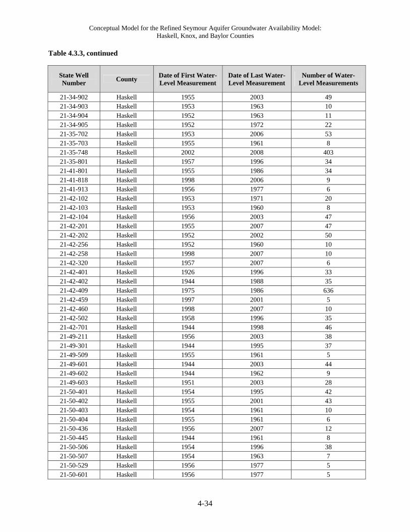
Conceptual Model for the Refined Seymour Aquifer Groundwater Availability Model: Haskell, Knox, and Baylor Counties
4-34
Table 4.3.3, continued
State Well Number
County Date of First Water-Level Measurement
Date of Last Water-Level Measurement
Number of Water-Level Measurements
21-34-902 Haskell 1955 2003 49 21-34-903 Haskell 1953 1963 10 21-34-904 Haskell 1952 1963 11 21-34-905 Haskell 1952 1972 22 21-35-702 Haskell 1953 2006 53 21-35-703 Haskell 1955 1961 8 21-35-748 Haskell 2002 2008 403 21-35-801 Haskell 1957 1996 34 21-41-801 Haskell 1955 1986 34 21-41-818 Haskell 1998 2006 9 21-41-913 Haskell 1956 1977 6 21-42-102 Haskell 1953 1971 20 21-42-103 Haskell 1953 1960 8 21-42-104 Haskell 1956 2003 47 21-42-201 Haskell 1955 2007 47 21-42-202 Haskell 1952 2002 50 21-42-256 Haskell 1952 1960 10 21-42-258 Haskell 1998 2007 10 21-42-320 Haskell 1957 2007 6 21-42-401 Haskell 1926 1996 33 21-42-402 Haskell 1944 1988 35 21-42-409 Haskell 1975 1986 636 21-42-459 Haskell 1997 2001 5 21-42-460 Haskell 1998 2007 10 21-42-502 Haskell 1958 1996 35 21-42-701 Haskell 1944 1998 46 21-49-211 Haskell 1956 2003 38 21-49-301 Haskell 1944 1995 37 21-49-509 Haskell 1955 1961 5 21-49-601 Haskell 1944 2003 44 21-49-602 Haskell 1944 1962 9 21-49-603 Haskell 1951 2003 28 21-50-401 Haskell 1954 1995 42 21-50-402 Haskell 1955 2001 43 21-50-403 Haskell 1954 1961 10 21-50-404 Haskell 1955 1961 6 21-50-436 Haskell 1956 2007 12 21-50-445 Haskell 1944 1961 8 21-50-506 Haskell 1954 1996 38 21-50-507 Haskell 1954 1963 7 21-50-529 Haskell 1956 1977 5 21-50-601 Haskell 1956 1977 5

Conceptual Model for the Refined Seymour Aquifer Groundwater Availability Model: Haskell, Knox, and Baylor Counties
4-35
Table 4.3.3, continued
State Well Number
County Date of First Water-Level Measurement
Date of Last Water-Level Measurement
Number of Water-Level Measurements
21-51-402 Haskell 1953 1958 5 21-51-422 Haskell 1951 1963 12 21-51-702 Haskell 1944 2003 44 21-51-703 Haskell 1951 1963 10 21-51-704 Haskell 1954 1961 6 21-51-705 Haskell 1951 1961 10 21-51-707 Haskell 1944 1961 8 21-51-710 Haskell 1951 1996 42 21-51-713 Haskell 1951 1963 11 21-51-721 Haskell 1956 1977 5 21-51-801 Haskell 1998 2006 11 21-20-901 Knox 1956 2003 42 21-27-801 Knox 1956 1998 41 21-27-904 Knox 1977 2007 10 21-27-905 Knox 1956 1977 5 21-27-913 Knox 1956 1977 5 21-28-301 Knox 1956 1963 7 21-28-401 Knox 1956 1977 5 21-28-814 Knox 1956 1977 5 21-29-102 Knox 1956 2003 44 21-33-901 Knox 1956 1994 30 21-33-940 Knox 1988 1996 8 21-34-202 Knox 1956 1996 37 21-34-218 Knox 1956 1977 5 21-34-402 Knox 1956 2003 47 21-34-501 Knox 1951 2003 36 21-34-601 Knox 1958 1996 35 21-34-602 Knox 1955 1977 9 21-34-603 Knox 1955 1963 7 21-34-801 Knox 1954 1960 6 21-34-802 Knox 1944 1961 10 21-35-102 Knox 1955 1980 26 21-35-103 Knox 1955 1960 5 21-35-104 Knox 1955 1961 7 21-35-201 Knox 1956 2003 42 21-35-301 Knox 1954 2003 44 21-35-401 Knox 1953 1961 8 21-35-402 Knox 1955 1993 36 21-35-501 Knox 1955 2000 43 21-35-502 Knox 1955 1996 36 21-35-503 Knox 1958 1962 5 21-35-602 Knox 1954 2003 39

Conceptual Model for the Refined Seymour Aquifer Groundwater Availability Model: Haskell, Knox, and Baylor Counties
4-36
Table 4.3.3, continued
State Well Number
County Date of First Water-Level Measurement
Date of Last Water-Level Measurement
Number of Water-Level Measurements
21-35-603 Knox 1953 1960 5 21-36-103 Knox 1975 1986 191 21-36-201 Knox 1952 2003 49 21-36-243 Knox 1998 2007 10 21-36-302 Knox 1953 1963 10 21-36-303 Knox 1944 1988 34 21-36-401 Knox 1951 1982 24 21-36-501 Knox 1954 1994 42 21-36-502 Knox 1956 1964 5 21-41-436 Stonewall 1982 2008 24
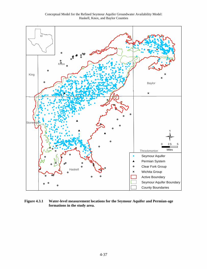
Conceptual Model for the Refined Seymour Aquifer Groundwater Availability Model: Haskell, Knox, and Baylor Counties
4-37
##
##
#
@
@
@
@
@
@
@
@
@
@
@
@
@
@
@
@
@
@
@
@
@
@
@
@@@
@
@
@
@
@
@
@@
@ @
@
@@@
@@
@
@@
@
@
@@
@
@
@
@
@@
@
@
@
@
Ï
Ï
Ï
!
!
!
!
!
!
!
!
!
!
!
!
!
!
!
!
!
!
!
!!!
!
!
!
!!
!
!!
!
!
!!
!
!
!
!! !
!
!
!
!
!!!!!
!!
!
!
!
!
!
!
!!
!!!!!!
!
!!
!
!!
! !
!!
!
!
!
!
!
!!!!
!!!!!
!
!!!
!!
!
!!!
!!
!!!!
!!
!
!
! !
! !
!!!
!
!
!!
! !
!
!!
!
!!
!
!!!
!
!!!!
!
!
!!
!
!
! !
! !!
!!
!!
!!
!!
!!!
!!!
!
!
!
!
! ! !!
!
!
!
!
!
!
!!!!
!
!
!
!
!!
!!
!!
!
! !!!!
!
!!!
!
!!
!!
!
!!!
!
!
! !!!!
!!!
!!!!!!!!!!!!
! !
!!!!
!!
!!
!
!
!!
!
!
!!
!
!
!!!!
!!
!
!
!
!!
!!
!
!
!
!
!!!
!
!
!!!
! !!
!!
!
!
!
!
!
!
!!
!!
!
!
!
!
!
!
!
!
! !!
!
!
!!
!
!
!
!
!
!
!
!
!
!!
!!
!
!
!
!
!
!
!
!
!
!
!
!
!
! !!
!
!
!
!!
!
!
!!
!
!
!
!!
!
!
!
!
!
! !
!
!
!!
!!
!
!
!
! !
!
!
!
!
!
!
!
!
!
!
!
!
!
!
!!!
!
!
!
!
!
!
!
!
!
!!
!
!
!
!
!
!
!
!
!
!!
!
!
!
!
!!
!
!
! !
!
!
!
!
!
!
!
!
!
!
! !!
!
!
!
!
!
! !
!
!!!!!
!
!
!!!
!
! !
!!
!!!
! !
!
!
!!
!
!
!! !
!
!
!
!!
!!
!
!
!
!
!
!
!
!
!
!
!
!!
!
!! !
!
!
!
!
!
!
! !!!!
!
!
!!
! !!
!!
!! !
!
!
!! !
!!
!!
!
!
!
!
!
!!
!
!
!
!
!
!
!
!
!
!
!
! !!
!
!
!
! !
!!!!
!!!
! !
!
!
!
!
!
!
! !
!
!
!
!
!
!
! !
!
!
! !!
!
!
!
!
!
!
!
!
!
!
!
!
!!
!!
!
!
!
!
!
!
!
!
!
!!! !!
! !
!
!
!
!
!!
!
!
!
!
!
!
!
!
!
!
!
! !
!!!
!
!
!
!!
!
!
!
!
!
!
!!
!
!
!
!
!
!
!!!
!
!
!
!
!
!
!!
!
!
!
!
!
!
!
!
!
!
!!
!
!
!
!
!
!
!
!
!
!!
! !
!!
!
!
!
!
!
!
!!
!
!
!!!
!
!
!
!
!!
! !
!!
!
!
!
!
!
!
!
!!
!
!!
!
!
!
!!
!
!
!
!
!
!!
!
!
!
!
!!!
!!
!
!
!
! !!!!
!
!
!
!!
!
!
!
!
!
!!
!!
!
!
!
!!!
!
!
! !
!
!
!
!
!
!
!
!
!
!
!
!
!
!
!
!
!!
!
!!
!
!
!
!
!
!
!
!
!
!!
!
!
!
! !
!
!
!!
!
!
!
!
!
!
!
!
!
!
!!
!
!
!
!
!
!
!
!
!
!
!
!
!
!
!
! !
!
!
!
!
!
!!!
!
!
!
!
!
!
!
!
!
!
!
!
! !
! !!
!
!
!
!
! !
!
!
!
!
!
!
!
!!
!
!
!
!
! !
!
!
!
!
!
!
!
!
!
!
!
!
!
!
!
!
! !
!!!!!!!
!
!!
!
!!
! !!
!
!!
!! ! !!!
! !!
!
!
!
!
!!
!
!
!
!!
!
!
!
!
!
! !
!
!
!!
!
!!
!
!
!
!
!
!
!
!
!!
!!
!
!
!
!
!
!
!
!
!
!!
!
!
!
!
!
!
!
!
!
!
!
!
!
!
!
!
!
!
!
!!
!
!
!!
!
!
!!
!
!
!!
!
!
!
!
!!
!
!
!
!
!
!
!!
!
!
!
!
!
!
!!
!
!
!
!!
!
!!
!
!
!!
!
!
!
!
!!
!
!!!
!
!
!
!
!
!
!
!
!
!!
!
!
!!
!!
!
!
!!
!
!
!!!!! !
!
!!
!
!
!!
!
!
!!
!
!
!
!
!
!
!
!!
!
!
!
!!
!
!
!
!
!!
!!
!
!
!
!
!
!
!
!
!
!
!!
!
!
!
!!!
!
!!
!
!
!
!
!
!
!
!
!
!!! !
!
!
!
!
!
!
!
!
!
!
!!!
!!
!
!
!
!!
!
!
! !
!!
!
!
!
!!
!!
!
!
!
!
!
!
!
!
!
!
!!
!
!
!
!
!
!
!
!
!!!
!
!!
!!
!!
!
!
!
!
!
!
!
!
!
!!
!
!!
!!
!
!
!!
!!
!
!!
!
!
!
!
!
!
!
!
!
!
!
!
!
!
!
!
!
!
!
!!
!
!
!!
!
!
!
!
!
!
!
!
!
!
!
!
! !
!!
!!
!
!
!!
!
!
!
!
!
!
!
!! !!
!
!
!
!
!
!!
!
!
!
!
!
!
!
!
!
!
!
!
!
!
!
!
!
!
!
!
!!
!
!
! !
!
!
!
!
!!
!
!
!
!
!
!
!
! !
! !!
!
!
!
!
! !
!
!
!
!
!
!!
!
!
!!
!
!
!
!
!
!!
!
!
!
!
!!!!
!
!
!
!
!!
!
!
!
!
!!
!
!!
!!!
!
!
!!
!
!
!
!
!
!!! !
!!
!
!!!!
!!
!
!
!
!!!
!
!
!
! ! !
!
!
!!!
!
!!
!
!
!
!
!
!
!
!
!
!
!
!
! !
! !!
!
!!!
!
!
!
!
!
!
!
!
!
!
!
!
!
!
!
!
!
!!
!
!
!
!
!
!
!
!
!!!!!
!
Knox
King
Haskell
Stonewall
Throckmorton
Baylor
0 2.5 5
Miles
! Seymour Aquifer
# Permian System
@ Clear Fork Group
Ï Wichita Group
Active Boundary
Seymour Aquifer Boundary
County Boundaries
Figure 4.3.1 Water-level measurement locations for the Seymour Aquifer and Permian-age formations in the study area.

Conceptual Model for the Refined Seymour Aquifer Groundwater Availability Model: Haskell, Knox, and Baylor Counties
4-38
0
50
100
150
200
250
300
350
400
450
500
550
Num
ber
of W
ate
r-L
eve
l Mea
sure
men
ts
1900 1910 1920 1930 1940 1950 1960 1970 1980 1990 2000 2010Year
Knox County
0
50
100
150
200
250
300
350
400
450
500
Nu
mbe
r o
f Wa
ter-
Le
vel M
ea
sure
me
nts
1900 1910 1920 1930 1940 1950 1960 1970 1980 1990 2000 2010Year
Baylor County
0
50
100
150
200
250
300
350
400
450
500
550
600
650
700
750
800
850
900
950
Num
ber
of W
ate
r-L
eve
l Me
asu
rem
en
ts
1900 1910 1920 1930 1940 1950 1960 1970 1980 1990 2000 2010Year
All Counties
0
50
100
150
200
250
300
350
400
450
500
Nu
mbe
r of W
ate
r-L
eve
l Me
asu
rem
en
ts
1900 1910 1920 1930 1940 1950 1960 1970 1980 1990 2000 2010Year
Haskell County
Figure 4.3.2 Temporal distribution of water-level measurements in the Seymour Aquifer in the study area.

Conceptual Model for the Refined Seymour Aquifer Groundwater Availability Model: Haskell, Knox, and Baylor Counties
4-39
Figure 4.3.3 Water-level rises reported in the Seymour Formation in western Haskell County by Bandy (1934) (from R.W. Harden and Associates, 1978).
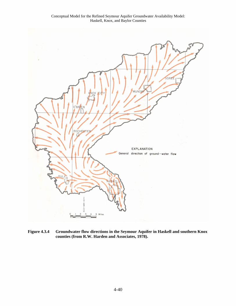
Conceptual Model for the Refined Seymour Aquifer Groundwater Availability Model: Haskell, Knox, and Baylor Counties
4-40
Figure 4.3.4 Groundwater flow directions in the Seymour Aquifer in Haskell and southern Knox counties (from R.W. Harden and Associates, 1978).

Conceptual Model for the Refined Seymour Aquifer Groundwater Availability Model: Haskell, Knox, and Baylor Counties
4-41
!
!
!
!
!
Knox
King
Haskell
Sto
new
all
Throckmorton
Baylor
1405
1375
1560
1268
1280
0 2.5 5
Miles
! Historical Spring
Active Boundary
Seymour Aquifer Boundary
County Boundaries
1296 Spring Elevation (feet)
Figure 4.3.5 Elevations of springs flowing from the Seymour Aquifer under steady-state conditions.

Conceptual Model for the Refined Seymour Aquifer Groundwater Availability Model: Haskell, Knox, and Baylor Counties
4-42
!
!
!
Knox
King
Haskell
Stonewall
Throckmorton
Baylor
1550
1575
1500
1525
14
75
1400
1600
145
0 1425
1625
13
75
13
00
1325
1350
1275
0 2.5 5
Miles
! Measurement Point
Active Boundary
County Boundaries
Contour Interval = 25 feet
Figure 4.3.6 Estimated steady-state water-level elevation contours for the Permian-age formations in the study area.

Conceptual Model for the Refined Seymour Aquifer Groundwater Availability Model: Haskell, Knox, and Baylor Counties
4-43
CC
C
C C
C
C
C
C
CC C
C
C
C
C
CC
C
C
C
C
C
C
C
C
C
C
CC
BB
B
B B
B
B
B
BB
B
B
BB
BB
B
BB
B
B
B
BB
BB
B
B
B
BB
BB
BB
B
B
BB
BB
B
B
A
A
A
A
A A
A
A
A
A
AA
A
A
AA
AA
A
A
A
AA
A
A
A
AA
AA
AA
AA
AA
A
A
A
A
AA
A
A
AA
AA
A
A
A
!
!
!
!
!
!!
!!!!
!
!
!
!
!
!
!
!
!
!
!
!
!
!
!
!
!
!!
KingKnox
Jones
Cottle
Young
Fisher
Archer
Baylor
Haskell
Foard
Wilbarger
Stephens
Stonewall
Wichita
Shackelford
Hardeman
Throckmorton
0 5 10 15
Miles
Study Area
Active Boundary
County Boundaries
Permian Water-LevelMeasurement Points
! Steady State
A 1980
B 1990
C 1997
Figure 4.3.7 Locations of data points used to develop estimated steady-state, 1980, 1990, and 1997 water-level elevation contours for the Permian-age formations.

Conceptual Model for the Refined Seymour Aquifer Groundwater Availability Model: Haskell, Knox, and Baylor Counties
4-44
!!
! !
!
!
!
!
!
!
!
!
!
!
!
!!
!
!
!
!
!! !
! !
!
!
!
! !!
!
!
! !
!
!
!
!
!
!
!! !!
!
!
!
Knox
King
Haskell
Stonewall
Throckmorton
Baylor
1470
1490
1460
1480
1500
1450
14301440
1510 15201530 1540
1550 1560
1410
1570 1580
1610
1600
1590
163
0
13
40
133
0
13
10
1320
1300
129
0
13
60
1280
1640
1400
1270
13
801390
1620
1420
1370
138
0
1390
1390
157
01610
1390
1590
1300
158
0
160
0
1380
156
0
1580
161
0
1400
0 2.5 5
Miles
! Measurement Point
Active Boundary
Seymour Aquifer Boundary
County Boundaries
Contour Interval = 10 feet
Figure 4.3.8 Estimated water-level elevation contours in the Seymour Aquifer in the study area at the start of the transient model calibration period (January 1980).

Conceptual Model for the Refined Seymour Aquifer Groundwater Availability Model: Haskell, Knox, and Baylor Counties
4-45
!
! !
!
!
!
!
!
!
!
!
!
!
!
!
!! !
!
!
!
Knox
King
Haskell
Stonewall
Throckmorton
Baylor
1490
1480
1470
1500
1460
15101520
1440
1430
1450
1530
15401550
1560
1590
1420
1570
1580
134
0
130013
20
13
30 1
31
013
50
136
0 1290
1410
13
80
1280
1620
1400
139
01610
1600
13
70
1600
1570
1320
15
70
1580
1410
1400
158
014
10
1590
1300
0 2.5 5
Miles
! Measurement Point
Active Boundary
Seymour Aquifer Boundary
County Boundaries
Contour Interval = 10 feet
Figure 4.3.9 Estimated water-level elevation contours in the Seymour Aquifer in the study area at the middle of the transient model calibration period (January 1990).
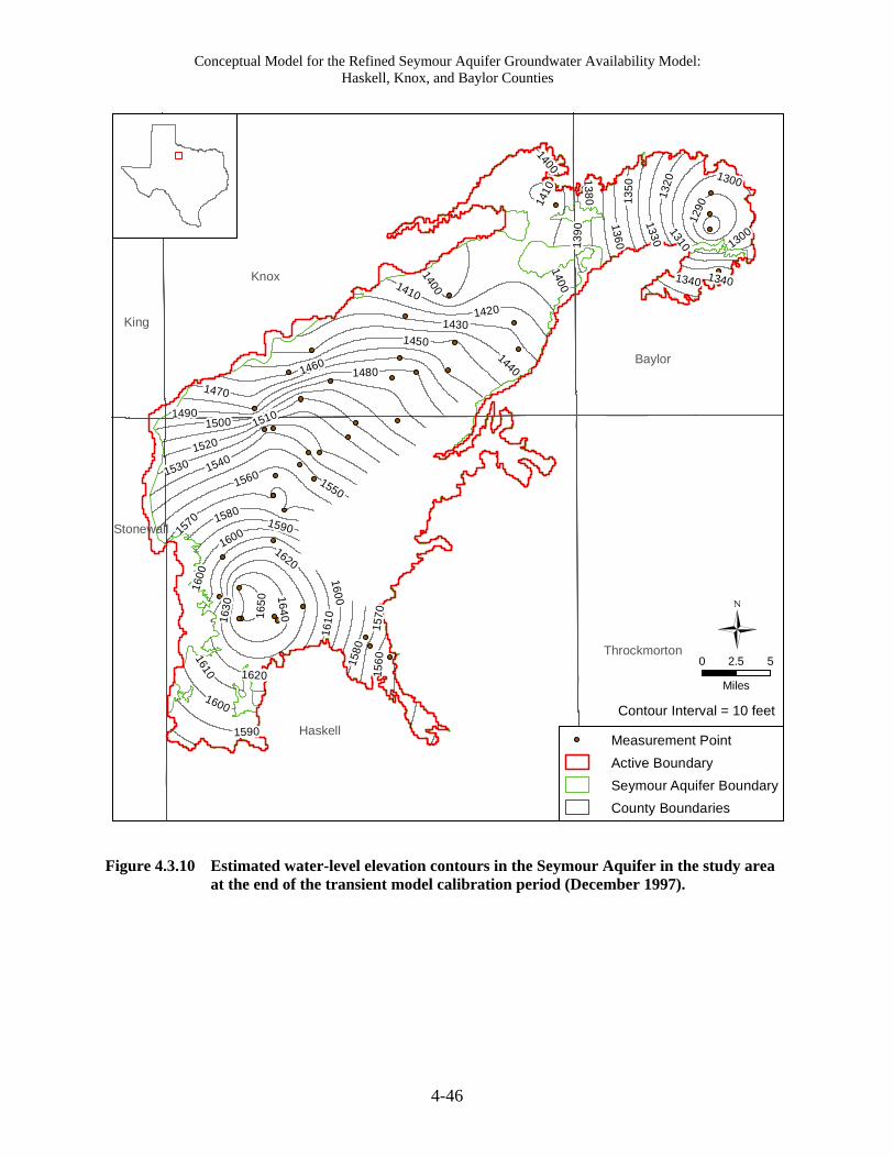
Conceptual Model for the Refined Seymour Aquifer Groundwater Availability Model: Haskell, Knox, and Baylor Counties
4-46
Knox
King
Haskell
Stonewall
Throckmorton
Baylor
1470
14601480
1500
1450
1490
1440
1430
1510
1520
1530 1540
1550
1420
1560
1570 1580
1590
1600
163
0
1320
1330
1310
13
50
1340
164
0
1360
1290
16
50
1400
13
80
1410
1300
13
90
1620
161
0
1620
1300
1600
1340
1600
1410
1610 15
60
1600
1400
1590
158
0
157
0
1400
0 2.5 5
Miles
Measurement Point
Active Boundary
Seymour Aquifer Boundary
County Boundaries
Contour Interval = 10 feet
Figure 4.3.10 Estimated water-level elevation contours in the Seymour Aquifer in the study area at the end of the transient model calibration period (December 1997).
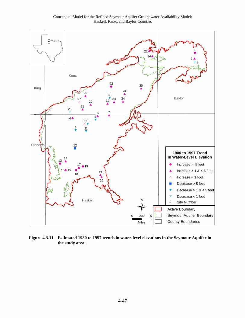
Conceptual Model for the Refined Seymour Aquifer Groundwater Availability Model: Haskell, Knox, and Baylor Counties
4-47
"
#
#
#
#
#
B
B
B
B
B
#
# #
#
#
#
#
#
#
#
#
#
#
#
#
#
##
!!
!
!
!
!
Knox
King
Haskell
Stonewall
Throckmorton
Baylor
1
4
2
76
9
3
8
5
17
23
13
19
18
3329
31
14
26
24
32
22
21
28
35
16
20
34
15
27
25
11
30
10
12
0 2.5 5
Miles
Active Boundary
Seymour Aquifer Boundary
County Boundaries
1980 to 1997 Trendin Water-Level Elevation
! Increase > 5 feet
# Increase > 1 & < 5 feet
B Increase < 1 foot
" Decrease > 5 feet
#
Decrease > 1 & < 5 feet
B
Decrease < 1 foot
Site Number2
Figure 4.3.11 Estimated 1980 to 1997 trends in water-level elevations in the Seymour Aquifer in the study area.

Conceptual Model for the Refined Seymour Aquifer Groundwater Availability Model: Haskell, Knox, and Baylor Counties
4-48
!
!
!!
!!
Knox
King
Haskell
Stonewall
Throckmorton
Baylor
14
75
15
25
15
00
13
75
160
0127
5
132
5
14
25
155
0
14
00
130
0
14
50
13
50
157
5
1425
1575
14
25
1450
1400 1375
13
50
0 2.5 5
Miles
! Measurment Point
Active Boundary
County Boundaries
Contour Interval = 25 feet
Figure 4.3.12 Estimated water-level elevation contours in the Permian-age formations in the study area at the start of the transient model calibration period (January 1980).

Conceptual Model for the Refined Seymour Aquifer Groundwater Availability Model: Haskell, Knox, and Baylor Counties
4-49
!
!
!
!
!
Knox
King
Haskell
Stonewall
Throckmorton
Baylor
14
75
152
5
15
00
157
5
160
0
1350
1275
1325
1300
137
5
14
25
14
00
155
0
14
50
137
5
1575
1375142
5
1400
0 2.5 5
Miles
! Measurement Point
Active Boundary
County Boundaries
Contour Interval = 25 feet
Figure 4.3.13 Estimated water-level elevation contours in the Permian-age formations in the study area at the middle of the transient model calibration period (January 1990).

Conceptual Model for the Refined Seymour Aquifer Groundwater Availability Model: Haskell, Knox, and Baylor Counties
4-50
!
!
Knox
King
Haskell
Stonewall
Throckmorton
Baylor
155
0
15
00
152
5
1575
14
75
1450
160
0
1375
1425
1400
1300 127
5
1325
1350
1450
1425
14
75
0 2.5 5
Miles
! Measurement Point
Active Boundary
County Boundaries
Contour Interval = 25 feet
Figure 4.3.14 Estimated water-level elevation contours in the Permian-age formations in the study area at the end of the transient model calibration period (December 1997).

Conceptual Model for the Refined Seymour Aquifer Groundwater Availability Model: Haskell, Knox, and Baylor Counties
4-51
! E@
"#
#
+Ï
!"+Ï!"
+Ï[#
1940 1945 1950 1955 1960 1965 1970 1975 1980Year
1600
1610
1620
1630
1640
1650
1660
1670
1680
1690
1700
Wa
ter-
Leve
l Ele
vatio
n (f
eet)
21-49-907 - Seymour Aquifer
21-49-906 - Seymour Aquifer
21-49-606 - Seymour Aquifer
21-49-903 - Seymour Aquifer
21-49-901 - Clear Fork Group
21-49-902 - Clear Fork Group
21-49-801 - Clear Fork Group
1940 1945 1950 1955 1960 1965 1970 1975 1980Year
1270
1280
1290
1300
1310
1320
1330
1340
1350
1360
1370
Wa
ter-
Leve
l Ele
vatio
n (f
eet)
21-29-306 - Seymour Aquifer
21-29-310 - Seymour Aquifer
21-29-307 - Seymour Aquifer
21-29-302 - Seymour Aquifer
21-29-311 - Clear Fork Group
1940 1945 1950 1955 1960 1965 1970 1975 1980Year
1270
1280
1290
1300
1310
1320
1330
1340
1350
1360
1370
Wa
ter-
Leve
l Ele
vatio
n (f
eet)
21-30-110 - Seymour Aquifer
21-30-118 - Seymour Aquifer
21-30-121 - Seymour Aquifer
21-30-109 - Seymour Aquifer
21-30-124 - Seymour Aquifer
21-30-119 - Clear Fork Group
Figure 4.3.15 Comparison of water-level elevations in the Seymour Aquifer and underlying Clear Fork Group in the study area.

Conceptual Model for the Refined Seymour Aquifer Groundwater Availability Model: Haskell, Knox, and Baylor Counties
4-52
!
!!
!! !!!!
!!!
!!
!!!
!!
!!
!
!!
!!
!!!
!! !!!
!
!!
!!
!
!
!!!!
!
!
!
!
!! !!
!!
!! !!
!
!
!
!!
!
!
!
!
!
!!!!!!
!
!!
!!!!!
!! !
!
!
!
!
!
!
!!
!
!
!
!
!
!
!
!
!
!
!
! !
!
!
!
!
!
!
!
!
!
!
!
!
!
!
!
!
!
!
!
!
!
!
!
!
!
!
! !
Knox
King
Haskell
Stonewall
Throckmorton
Baylor
0 2.5 5
Miles
! Transient Data Locations
Active Boundary
Seymour Aquifer Boundary
County Boundaries
Figure 4.3.16 Locations of Seymour Aquifer wells in the study area with transient water-level data.

Conceptual Model for the Refined Seymour Aquifer Groundwater Availability Model: Haskell, Knox, and Baylor Counties
4-53
!! !
!!
1920 1930 1940 1950 1960 1970 1980 1990 2000 2010Date
1300
1305
1310
1315
1320
1325
1330
1335
1340
1345
1350
Wa
ter-
Leve
l Ele
vatio
n (
fee
t)
21-22-701Baylor County
base of well
1920 1930 1940 1950 1960 1970 1980 1990 2000 2010Date
1280
1285
1290
1295
1300
1305
1310
1315
1320
1325
1330
Wa
ter-
Leve
l Ele
vatio
n (
fee
t)
21-22-703Baylor County
base of well
1920 1930 1940 1950 1960 1970 1980 1990 2000 2010Date
1250
1255
1260
1265
1270
1275
1280
1285
1290
1295
1300
Wa
ter-
Leve
l Ele
vatio
n (
fee
t)
21-22-802Baylor County
base of well
1920 1930 1940 1950 1960 1970 1980 1990 2000 2010Date
1250
1255
1260
1265
1270
1275
1280
1285
1290
1295
1300
Wa
ter-
Leve
l Ele
vatio
n (
fee
t)
21-30-202Baylor County
base of well
1920 1930 1940 1950 1960 1970 1980 1990 2000 2010Date
1250
1255
1260
1265
1270
1275
1280
1285
1290
1295
1300
Wa
ter-
Leve
l Ele
vatio
n (
fee
t)
21-30-204Baylor County
base of well
Figure 4.3.17 Hydrographs for the five Seymour Aquifer wells in Baylor County with long-term transient water-level data.

Conceptual Model for the Refined Seymour Aquifer Groundwater Availability Model: Haskell, Knox, and Baylor Counties
4-54
!!
!
!
!!
1920 1930 1940 1950 1960 1970 1980 1990 2000 2010Date
1490
1495
1500
1505
1510
1515
1520
1525
1530
1535
1540
1545
1550W
ate
r-Le
vel E
leva
tion
(fe
et)
21-42-202Haskell County
base of well
1920 1930 1940 1950 1960 1970 1980 1990 2000 2010Date
1480
1485
1490
1495
1500
1505
1510
1515
1520
1525
1530
Wa
ter-
Leve
l Ele
vatio
n (
fee
t)
21-35-702Haskell County
base of well
1920 1930 1940 1950 1960 1970 1980 1990 2000 2010Date
1490
1495
1500
1505
1510
1515
1520
1525
1530
1535
1540
Wa
ter-
Leve
l Ele
vatio
n (
fee
t)
21-34-902Haskell County
base of well
1920 1930 1940 1950 1960 1970 1980 1990 2000 2010Date
1520
1525
1530
1535
1540
1545
1550
1555
1560
1565
1570
1575
1580
Wa
ter-
Leve
l Ele
vatio
n (
fee
t)
21-42-104Haskell County
base of well
1920 1930 1940 1950 1960 1970 1980 1990 2000 2010Date
1600
1605
1610
1615
1620
1625
1630
1635
1640
1645
1650
Wa
ter-
Leve
l Ele
vatio
n (
fee
t)
21-50-402Haskell County
base of well
1920 1930 1940 1950 1960 1970 1980 1990 2000 2010Date
1560
1565
1570
1575
1580
1585
1590
1595
1600
1605
1610
1615
1620
Wa
ter-
Le
vel E
leva
tion
(fe
et)
21-49-211Haskell County
base of well
Figure 4.3.18 Example hydrographs showing fluctuating water-level elevations with time in the Seymour Aquifer in Haskell County.

Conceptual Model for the Refined Seymour Aquifer Groundwater Availability Model: Haskell, Knox, and Baylor Counties
4-55
!
!
!
!
!
!
1920 1930 1940 1950 1960 1970 1980 1990 2000 2010Date
1500
1505
1510
1515
1520
1525
1530
1535
1540
1545
1550W
ate
r-Le
vel E
leva
tion
(fe
et)
21-34-702Haskell County
base of well
1920 1930 1940 1950 1960 1970 1980 1990 2000 2010Date
1450
1455
1460
1465
1470
1475
1480
1485
1490
1495
1500
Wa
ter-
Leve
l Ele
vatio
n (
fee
t)
21-35-801Haskell County
base of well
1920 1930 1940 1950 1960 1970 1980 1990 2000 2010Date
1540
1545
1550
1555
1560
1565
1570
1575
1580
1585
1590
1595
1600
Wa
ter-
Leve
l Ele
vatio
n (
fee
t)
21-42-401Haskell County
base of well
1920 1930 1940 1950 1960 1970 1980 1990 2000 2010Date
1550
1555
1560
1565
1570
1575
1580
1585
1590
1595
1600
Wa
ter-
Leve
l Ele
vatio
n (
fee
t)
21-41-801Haskell County
base of well
1920 1930 1940 1950 1960 1970 1980 1990 2000 2010Date
1540
1545
1550
1555
1560
1565
1570
1575
1580
1585
1590
Wa
ter-
Leve
l Ele
vatio
n (
fee
t)
21-51-702Haskell County
base of well
1920 1930 1940 1950 1960 1970 1980 1990 2000 2010Date
1610
1615
1620
1625
1630
1635
1640
1645
1650
1655
1660
Wa
ter-
Leve
l Ele
vatio
n (
fee
t)
21-49-301Haskell County
base of well
Figure 4.3.19 Example hydrographs showing increasing and stable water-level elevations with time in the Seymour Aquifer in Haskell County.
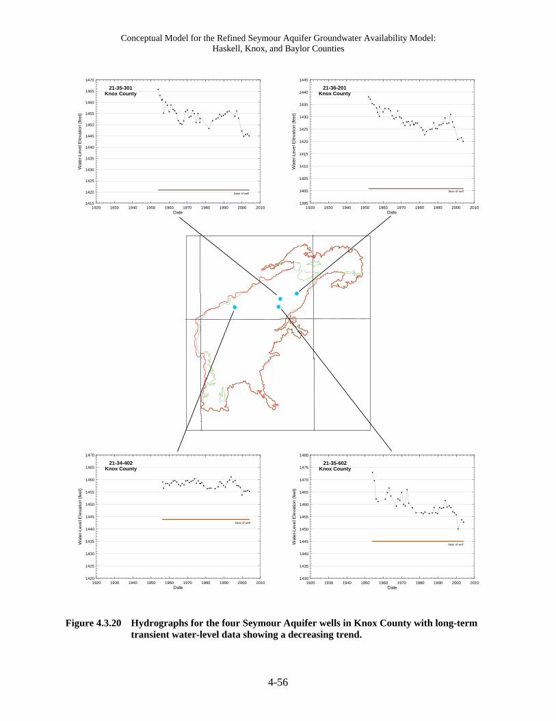
Conceptual Model for the Refined Seymour Aquifer Groundwater Availability Model: Haskell, Knox, and Baylor Counties
4-56
!
!
!
!
1920 1930 1940 1950 1960 1970 1980 1990 2000 2010Date
1395
1400
1405
1410
1415
1420
1425
1430
1435
1440
1445
Wa
ter-
Le
vel E
leva
tion
(fe
et)
21-36-201Knox County
base of well
1920 1930 1940 1950 1960 1970 1980 1990 2000 2010Date
1430
1435
1440
1445
1450
1455
1460
1465
1470
1475
1480
Wa
ter-
Le
vel E
leva
tion
(fe
et)
21-35-602Knox County
base of well
1920 1930 1940 1950 1960 1970 1980 1990 2000 2010Date
1415
1420
1425
1430
1435
1440
1445
1450
1455
1460
1465
1470W
ate
r-Le
vel E
leva
tion
(fe
et)
21-35-301Knox County
base of well
1920 1930 1940 1950 1960 1970 1980 1990 2000 2010Date
1420
1425
1430
1435
1440
1445
1450
1455
1460
1465
1470
Wa
ter-
Le
vel E
leva
tion
(fe
et)
21-34-402Knox County
base of well
Figure 4.3.20 Hydrographs for the four Seymour Aquifer wells in Knox County with long-term transient water-level data showing a decreasing trend.

Conceptual Model for the Refined Seymour Aquifer Groundwater Availability Model: Haskell, Knox, and Baylor Counties
4-57
!
!! ! !
1920 1930 1940 1950 1960 1970 1980 1990 2000 2010Date
1435
1440
1445
1450
1455
1460
1465
1470
1475
1480
1485W
ate
r-L
eve
l Ele
vatio
n (
fee
t)21-35-201
Knox County
base of well
1920 1930 1940 1950 1960 1970 1980 1990 2000 2010Date
1450
1455
1460
1465
1470
1475
1480
1485
1490
1495
1500
Wa
ter-
Le
vel E
leva
tion
(fe
et)
21-35-502Knox County
base of well
1920 1930 1940 1950 1960 1970 1980 1990 2000 2010Date
1410
1415
1420
1425
1430
1435
1440
1445
1450
1455
1460
Wa
ter-
Le
vel E
leva
tion
(fe
et)
21-36-501Knox County
base of well
1920 1930 1940 1950 1960 1970 1980 1990 2000 2010Date
1460
1465
1470
1475
1480
1485
1490
1495
1500
1505
1510
Wa
ter-
Le
vel E
leva
tion
(fe
et)
21-35-501Knox County
base of well
1920 1930 1940 1950 1960 1970 1980 1990 2000 2010Date
1470
1475
1480
1485
1490
1495
1500
1505
1510
1515
1520
Wa
ter-
Le
vel E
leva
tion
(fe
et)
21-35-402Knox County
base of well
Figure 4.3.21 Hydrographs for the five Seymour Aquifer wells in Knox County with long-term transient water-level data showing a decreasing and then increasing trend.
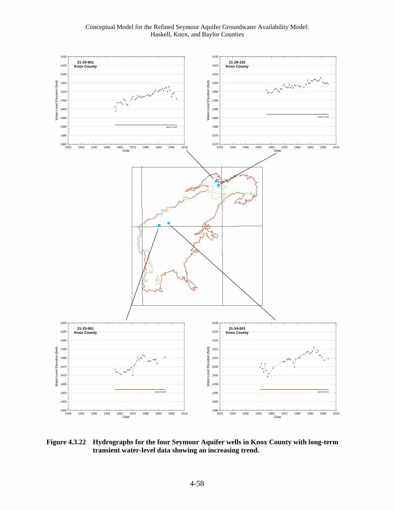
Conceptual Model for the Refined Seymour Aquifer Groundwater Availability Model: Haskell, Knox, and Baylor Counties
4-58
!!
!!
1920 1930 1940 1950 1960 1970 1980 1990 2000 2010Date
1450
1455
1460
1465
1470
1475
1480
1485
1490
1495
1500
Wa
ter-
Le
vel E
leva
tion
(fe
et)
21-33-901Knox County
base of well
1920 1930 1940 1950 1960 1970 1980 1990 2000 2010Date
1370
1375
1380
1385
1390
1395
1400
1405
1410
1415
1420
Wa
ter-
Le
vel E
leva
tion
(fe
et)
21-29-102Knox County
base of well
1920 1930 1940 1950 1960 1970 1980 1990 2000 2010Date
1380
1385
1390
1395
1400
1405
1410
1415
1420
1425
1430W
ate
r-L
eve
l Ele
vatio
n (
fee
t)
21-20-901Knox County
base of well
1920 1930 1940 1950 1960 1970 1980 1990 2000 2010Date
1480
1485
1490
1495
1500
1505
1510
1515
1520
1525
1530
Wa
ter-
Le
vel E
leva
tion
(fe
et)
21-34-501Knox County
base of well
Figure 4.3.22 Hydrographs for the four Seymour Aquifer wells in Knox County with long-term transient water-level data showing an increasing trend.

Conceptual Model for the Refined Seymour Aquifer Groundwater Availability Model: Haskell, Knox, and Baylor Counties
4-59
!
!
!
1920 1930 1940 1950 1960 1970 1980 1990 2000 2010Date
1400
1405
1410
1415
1420
1425
1430
1435
1440
1445
1450W
ate
r-L
eve
l Ele
vatio
n (
fee
t)
21-34-202Knox County
base of well
1920 1930 1940 1950 1960 1970 1980 1990 2000 2010Date
1390
1395
1400
1405
1410
1415
1420
1425
1430
1435
1440
Wa
ter-
Le
vel E
leva
tion
(fe
et)
21-27-801Knox County
base of well
1920 1930 1940 1950 1960 1970 1980 1990 2000 2010Date
1460
1465
1470
1475
1480
1485
1490
1495
1500
1505
1510
Wa
ter-
Le
vel E
leva
tion
(fe
et)
21-34-601Knox County
base of well
Figure 4.3.23 Hydrographs for the three Seymour Aquifer wells in Knox County with long-term transient water-level data showing a stable trend.

Conceptual Model for the Refined Seymour Aquifer Groundwater Availability Model: Haskell, Knox, and Baylor Counties
4-60
!
!
!
June 2002 June 2003 June 2004 June 2005 June 2006 June 2007 June 200
Date
1470
1475
1480
1485
1490
1495
1500
1505
1510
Wat
er-
Lev
el E
leva
tion
(fee
t)
Jan 2003 Jan-2004 Jan 2005 Jan 2006 Jan 2007 Jan 2008
21-35-748Haskell County
base of well
June 1975 Jan 1976 June 1976 Jan 1977 June 1977 Jan 1978Date
1430
1432
1434
1436
1438
1440
1442
1444
1446
1448
1450
1452
1454
1456
Wa
ter-
Leve
l Ele
vatio
n (
fee
t)
21-36-103Knox County
base of well
6/1975 6/1976 6/1977 6/1978 6/1979 6/1980 6/1981 6/1982 6/1983 6/1984 6/1985 6/1986
Date
1565
1570
1575
1580
1585
1590
1595
Wat
er -
Leve
l Ele
vatio
n (f
eet)
1/1976 1/1977 1/1978 1/1979 1/1980 1/1981 1/1982 1/1983 1/1984 1/1985 1/1986 1/1987
21-42-409Haskell County
base of well
Figure 4.3.24 Hydrographs for the three Seymour Aquifer wells with sufficient data to evaluate long-term seasonal fluctuations in water-level elevations.

Conceptual Model for the Refined Seymour Aquifer Groundwater Availability Model: Haskell, Knox, and Baylor Counties
4-61
Dec Jan Feb Mar Apr May Jun Jul Aug Sep Oct Nov Dec Jan Feb Mar
Date
1300
1305
1310
1315
1320
Wa
ter
-Le
vel E
leva
tion
(fe
et)
1968 1969 1969 1969 1969 1969 1969 1969 1969 1969 1969 1969 1969 1970 1970 1970
21-22-707 - Irrigation
21-22-904 - Domestic
21-30-106 - Irrigation
21-21-930 - Domestic
Dec Jan Feb Mar Apr May Jun Jul Aug Sep Oct Nov Dec Jan Feb Mar
Date
1264
1266
1268
1270
1272
1274
1276
Wa
ter
-Le
vel E
leva
tion
(fe
et)
1968 1969 1969 1969 1969 1969 1969 1969 1969 1969 1969 1969 1969 1970 1970 1970
21-30-332 - Irrigation
21-30-341 - Irrigation
Dec Jan Feb Mar Apr May Jun Jul Aug Sep Oct Nov Dec Jan Feb Mar
Date
1284
1286
1288
1290
1292
1294
1296
1298
1300
Wa
ter
-Le
vel E
leva
tion
(fe
et)
1968 1969 1969 1969 1969 1969 1969 1969 1969 1969 1969 1969 1969 1970 1970 1970
21-22-704 - Irrigation
21-22-801 - Irrigation
Dec Jan Feb Mar Apr May Jun Jul Aug Sep Oct Nov Dec Jan Feb Mar
Date
1366
1368
1370
1372
1374
1376
1378
1380
Wa
ter
-Le
vel E
leva
tion
(fe
et)
1968 1969 1969 1969 1969 1969 1969 1969 1969 1969 1969 1969 1969 1970 1970 1970
21-21-803 - Unused
21-29-305 - Industrial
Dec Jan Feb Mar Apr May Jun Jul Aug Sep Oct Nov Dec Jan Feb Mar
Date
1384
1386
1388
1390
1392
1394
Wa
ter
-Le
vel E
leva
tion
(fe
et)
1968 1969 1969 1969 1969 1969 1969 1969 1969 1969 1969 1969 1969 1970 1970 1970
21-29-103 - Stock
Dec Jan Feb Mar Apr May Jun Jul Aug Sep Oct Nov Dec Jan Feb Mar
Date
1324
1326
1328
1330
1332
1334
1336
Wa
ter
-Le
vel E
leva
tion
(fe
et)
1968 1969 1969 1969 1969 1969 1969 1969 1969 1969 1969 1969 1969 1970 1970 1970
21-21-902 - Stock
21-21-926 - Unused
21-21-801 - Stock
21-21-912 - Irrigation
G!
G GG # Ï#
Ï #
[! # %%
21-30-10621-29-305
21-21-803
21-29-103
21-21-80121-21-902
21-21-92621-21-912
21-21-930
21-22-707
21-22-70421-22-801
21-22-904
21-30-332
21-20-341
Figure 4.3.25 Hydrographs for the 15 Seymour Aquifer wells in Baylor County with data to evaluate seasonal fluctuations between December 1968 and February 1970.

Conceptual Model for the Refined Seymour Aquifer Groundwater Availability Model: Haskell, Knox, and Baylor Counties
4-62
This page is intentionally blank.


