

Copyright Warning & Restrictions
The copyright law of the United States (Title 17, United States Code) governs the making of photocopies or other
reproductions of copyrighted material.
Under certain conditions specified in the law, libraries and archives are authorized to furnish a photocopy or other
reproduction. One of these specified conditions is that the photocopy or reproduction is not to be “used for any
purpose other than private study, scholarship, or research.” If a, user makes a request for, or later uses, a photocopy or reproduction for purposes in excess of “fair use” that user
may be liable for copyright infringement,
This institution reserves the right to refuse to accept a copying order if, in its judgment, fulfillment of the order
would involve violation of copyright law.
Please Note: The author retains the copyright while the New Jersey Institute of Technology reserves the right to
distribute this thesis or dissertation
Printing note: If you do not wish to print this page, then select “Pages from: first page # to: last page #” on the print dialog screen

The Van Houten library has removed some of the personal information and all signatures from the approval page and biographical sketches of theses and dissertations in order to protect the identity of NJIT graduates and faculty.

ABSTRACT
USE OF FLUORESCENT MICROSPHERES TO MEASURE CORONARY
FLOW RESERVE IN RAT ANIMAL MODEL
by
Riddhi Harsh Shah
Heart attacks result from reduced or blocked blood flow through major coronary arteries,
resulting in permanent damage to heart muscle. Coronary blood flow (CBF) is thus
important to measure in experimental animal models of heart disease. A standard method
to measure CBF uses tracer microspheres (Ø = 15 µm) injected into the left ventricle that
flow through coronary arteries but cannot pass through capillaries and so become trapped
in heart muscle. Previously, radioactive or colored microspheres have quantified the
number of tracers trapped in the muscle. Fluorescent microspheres offer a more recent
and more sensitive measurement mode. However, fluorescent microspheres have not
often been used to measure CBF in small animals (rats, mice) that are now the most
common animal models used in heart research. This thesis aimed to develop the
techniques for use of fluorescent microspheres to measure CBF in rat animal models used
by the cell biology laboratories at UMDNJ-Newark. Two non-overlapping fluorescent
wavelengths were chosen (yellow-green; red). Using a spectrophotometer, fluorescence
intensity was calibrated for known numbers of microspheres (set via controlled dilution).
CBF in two rats was measured at rest and during maximal vasodilation (adenosine) using
procedures for colored microspheres. After euthanasia, hearts were removed, and blood
samples and left ventricular tissue were processed using a sedimentation method for full
recovery of fluorescent microspheres, which were scanned through the spectrophotometer
to count fluorescence intensity. Using the predetermined calibration curve, the number of
microspheres in each sample was determined; from this CBF was calculated. CBF
averaged 5.9 ml/min/g at rest, which was within the normal range for rats quoted in
recent literature. With maximal vasodilation, CBF increased to an average of 12.9
ml/min/g, which indicated a coronary flow reserve that was 2.2 times the resting level.
The same value for coronary flow velocity reserve (2.2) was measured in 6 rats using
Doppler echocardiography. The consistency of these results suggests that the procedures
developed for fluorescent microspheres lead to repeatable and reliable measurement of
coronary blood flow in rats.

USE OF FLUORESCENT MICROPSHERES TO MEASURE CORONARY
FLOW RESERVE IN RAT ANIMAL MODEL
by
Riddhi Harsh Shah
A Thesis
Submitted to the Faculty of
New Jersey Institute of Technology
In Partial Fulfillment of the Requirements for the Degree of
Master of Science in Biomedical Engineering
Department of Biomedical Engineering
August 2011

APPROVAL PAGE
USE OF FLUORESCENT MICROSPHERES TO MEASURE CORONARY
FLOW RESERVE IN MICE MODEL
Riddhi Harsh Shah
Dr. William Hunter, Thesis Advisor Date
Professor of Biomedical Engineering, NJIT
Dr. Van Buskirk, Thesis Advisor Date
Distinguished Professor and Chair of Biomedical Engineering, NJIT
Dr. Raquel Perez Castillejos, Committee member Date
Assistant Professor, NJIT
BIOGRAPHICAL SKETCH
Author: Riddhi Harsh Shah
Degree: Master of Science
Date: August 2011
Undergraduate and Graduate Education:
• Master of Science in Biomedical Engineering,New Jersey Institute of Technology, Newark, NJ, 2011
• Bachelor of Science in Biomedical Engineering,Mumbai University, Mumbai, India, 2009
Major: Biomedical Engineering

vi
Om NamahShivay!!!
I would like to dedicate this thesis to my parents and to all my friends. There is no doubt in my
mind that without their continuous support, blessings and encouragement I could not have
achieved this.
My strong belief and conviction in Almighty GOD and HIS grace has made my dreams come
true.

vii
ACKNOWLEDGMENT
I am deeply grateful to New Jersey Institute of Technology, Biomedical Engineering Department
for providing me with all the facilities to make this thesis successful.
I wish to express my sincere gratitude to my thesis advisor, Dr. William Hunter who
planned the subject, helped me, guided me and encouraged me through all the steps of my
academic work. I would like to thank him for his invaluable suggestions and comments,
immense patience and dedication that proved very valuable during this work. Without him, this
thesis would not have been accomplished.
I am really grateful to Dr. Stephen F Vatner, director of the Cellular Biology and
Molecular Medicine Department at the University of Medicine and Dentistry of New Jersey, for
allowing me to work in their cardiovascular research lab and complete my thesis. I owe my
special thanks to Dr. Xin Zhao for performing cannulation and microsphere injection procedures
in rats. Also, I am thankful to Dr. Shumin Gao for performing Doppler echocardiography studies
of coronary flow in rats and providing the data from those studies for comparison with my
fluorescent microsphere measurements. I owe my gratitude to Dr. Misun Park and her research
assistant, Grace Jung Lee, who taught me various immunohistochemistry procedures and showed
an active participation in my thesis. I thank them for helping me search for the references and
teach me to use the library and internet services. I thank Dr. S J Leibovich for teaching me how
to use the fluorescent spectrophotometer instrument. Also, I thank all his colleagues in the lab for
their coordination in allowing me to make fluorescent measurements in their lab.
I owe my special thanks to the additional members of my thesis committee, Dr. William
Van Buskirk and Dr. Raquel Perez Castillejos for supporting and appreciating my thesis work.

viii
Finally, I would like to thank my fellow students, my friends and my family whose constant
support, encouragement and advice has been a driving force behind the research.

ix
TABLE OF CONTENTS
Chapter Page
1 INTRODUCTION……............................………………..………………………….
1.1 Heart attack and coronary blood flow……………………………………………
1
1
1.2 Significance of coronary blood flow…..…………………………………….…...
1.3 Use of laboratory animals in biomedical research………………………………..
2
4
2
1.4 Techniques used previously to determine blood flow in rats and mice…………..
1.5 Use of Fluorescent Microsphere Methods to Determine Coronary Blood Flow
in Research Animals……………………………………………………………...
1.6 Calculation of myocardial blood flow by use of fluorescent microspheres……...
1.7 Use of Doppler echocardiography to determine coronary blood flow…………...
1.8 Specific aims of this thesis……………………………………………………….
DETERMINATION OF CALIBRATION CURVES FOR FLUORESCENT
MICROSPHERES………………………………………………………………….....
2.1 Principles of Fluorescence Spectrophotometry…………………………………..
2.2 Biotek Instruments FL 500 Microplate Reader…………………………………..
2.3 Fluorescence Spectra of Commercial Microbeads……………………………..
2.4 Choice of Fluorescent Dyes used in Microbeads………………………………
2.5 Choice of Excitation and Emission Filters……………………………………..
2.6 Determination of Calibration Curve……………………………………………...
2.7 Results of Calibration Curves………………………………………………...
2.8 Averaging Calibration Curves………………………………………………..
6
7
10
11
13
14
14
15
18
20
22
23
24
26
x
TABLE OF CONTENTS
(Continued)
Chapter Page
3
4
EXPERIMENTAL TECHNIQUES TO DETERMINE CORONARY BLOOD
FLOW IN RAT ANIMAL MODEL………………………………………………...
3.1 Source of fluorescent microspheres……………………………………………..
3.2 Calculation of number of microspheres for injection…………………………...
3.3 Preparation of fluorescent microspheres for injection…………………………..
3.4 Reference blood flow sampling…………………………………………………
3.5 Animals………………………………………………………………………….
3.6 Surgery………………………………………………………………………….
3.7 Procedure for injection of microspheres………………………………………...
EXPERIMENTAL TECHNIQUES TO RECOVER MICROSPHERES
FROM TISSUE AND BLOOD……………………………………………………...
4.1 Three alternative methods to separate microspheres from tissues……………...
4.2 Negative Pressure Filtration…………………………………………………….
4.3 Polyamide Woven Filtration Devices…………………………………………...
29
29
30
31
32
34
34
36
39
39
39
40
4.4 Sedimentation…………………………..……………………………………….
4.5 Importance of accurate fluid volumes…………………………………………..
41
42
4.6 Solutions used in the sedimentation method……………………………………
4.7 Calculation of centrifuge rotation rate…………………………………………..
4.8 Details of sedimentation procedure……………………………………………..
4.9 Advantages of the sedimentation method………………………………………
44
.
45
47
49

xi
TABLE OF CONTENTS
(Continued)
Chapter Page
5 INITIAL MEASUREMENTS OF CORONARY BLOOD FLOW AND
CORONARY RESERVE IN RATS USING FLUOROSCENT MICROSPHERES.
5.1 Summary of experimental protocol……………………………………………..
5.2 Measurement of microsphere number in tissue and blood samples………….…
5.3 Calculation of coronary blood flow and coronary flow reserve………………...
5.4 Comparison with coronary flow reserve measured using Doppler
Echocardiography……………………………………………………………….
6 DISCUSSION AND FUTURE WORK…………………………………………...
APPENDIX 1………………………………………………………………………..
APPENDIX 2………………………………………………………………………..
REFERENCES………………………………………………………………………
50
50
59
61
63
66
71
73
84
xii
LIST OF TABLES
Table Page
2.1 Filters providing best match to excitation and emission spectra……………....... 22
2.2
2.3
2.4
5.1
5.2
5.3
5.4
5.5
5.6
Typical calibration measurements for yellow-green microspheres…..………….
Summary of calibration for yellow-green microspheres………………………...
Summary of calibration for red microspheres…………………………………...
Timeline of a typical experiment………………………………………………...
Hemodynamic conditions during microsphere injections in rat 1……………….
Hemodynamic conditions during microsphere injections in rat 2……………….
Number of fluorescent microspheres in blood and tissue samples in rat 1…..….
Number of fluorescent microspheres in blood and tissue samples in rat 2……...
Measurement of coronary flow reserve using Doppler Echocardiography……...
25
27
28
51
58
58
61
61
65
xiii
LIST OF FIGURES
Figures Page
1.1
2.1
2.2
2.3
2.4
2.5
2.6
2.7
Coronary circulation in the heart…………………...……………………………
Microplate reader used for fluorescence spectroscopy…………………………
Selection of excitation and emission filters in Bio Tek FL500………..………..
Spectra of emission filters available in Bio Tek FL500……..…………………..
Spectra of excitation filters available in Bio Tek FL500...…………………….
Spectra of emitted fluorescence from a suite of commercial microbeads...……..
Excitation (blue) and emission (red) spectra for yellow – green dye...………….
Typical calibration regression line for yellow – green microspheres..………….
3
15
16
17
17
18
19
25
2.8
2.9
3.1
4.1
5.1
5.2
5.3
5.4
5.5
Linear regression calibration curves for yellow-green microspheres…..……….
Linear regression calibration curves for red microspheres……….…..………....
Rat model showing cannulation in left ventricle and femoral artery…….……...
Sedimentation procedure for fluorescent microspheres…..……………………..
Hemodynamic parameters at baseline in Rat 2………………………………….
Hemodynamic parameters during beginning of reference blood flow…….……
Hemodynamic parameters at beginning of injection……..……………………...
Hemodynamic parameters after re – stabilization …………………..…………..
Hemodynamic parameters after attaining steady state under adenosine…….…..
27
28
35
42
53
54
55
56
57

1
CHAPTER 1
INTRODUCTION
1.1 Heart Attack and Coronary Blood Flow
Heart disease and related conditions affect 12 million Americans and cost $274 billion a
year [5]. It is the leading cause of death in United States [5]. Unfortunately, many people
do not realize any potential problems with their heart until they have a heart attack. The
treatments are generally expensive. The patient has to undergo coronary bypass or
coronary angioplasty surgery. Today’s lifestyle, eating habits and drinking habits are the
major cause of heart attacks and stroke [5]. A heart attack occurs when blood vessels that
supply blood to the heart are blocked, preventing enough oxygen from getting to the
heart, resulting in death or permanent damage of heart muscle.
In atherosclerosis, plaque builds up in the walls of coronary arteries. This plaque
is made up of cholesterol and other cells. A heart attack can occur as a result of the
following:
1) The slow buildup of plaque may almost block one of the coronary arteries. A heart attack may occur if not enough oxygen-containing blood can flow through this blockage. This is more likely to happen during exercise. 2) The plaque itself develops cracks (fissures) or tears. Blood platelets stick to these tears and form a blood clot (thrombus). A heart attack can occur if this blood clot completely blocks the passage of oxygen-rich blood to the heart. This is the most common cause of heart attack.
3) Sudden, significant emotional or physical stress, including an illness, can trigger a heart attack, too.
Slow build up of plaque and blockage of coronary arteries is the cause of heart
attacks. Researchers say that there are two types of plaque: soft plaque, also known as
2
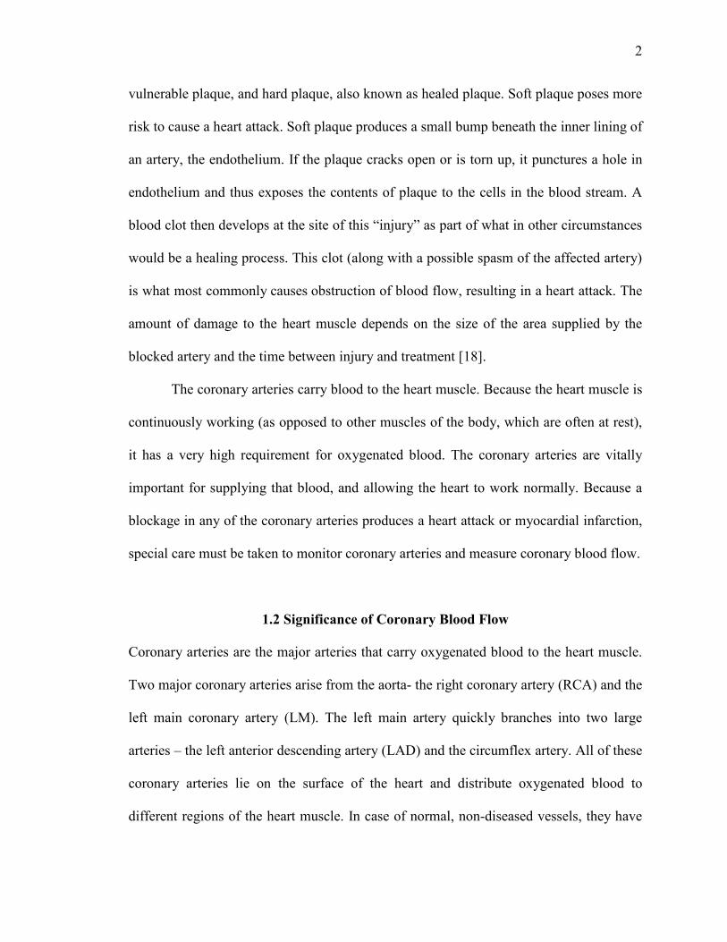
vulnerable plaque, and hard plaque, also known as healed plaque. Soft plaque poses more
risk to cause a heart attack. Soft plaque produces a small bump beneath the inner lining of
an artery, the endothelium. If the plaque cracks open or is torn up, it punctures a hole in
endothelium and thus exposes the contents of plaque to the cells in the blood stream. A
blood clot then develops at the site of this “injury” as part of what in other circumstances
would be a healing process. This clot (along with a possible spasm of the affected artery)
is what most commonly causes obstruction of blood flow, resulting in a heart attack. The
amount of damage to the heart muscle depends on the size of the area supplied by the
blocked artery and the time between injury and treatment [18].
The coronary arteries carry blood to the heart muscle. Because the heart muscle is
continuously working (as opposed to other muscles of the body, which are often at rest),
it has a very high requirement for oxygenated blood. The coronary arteries are vitally
important for supplying that blood, and allowing the heart to work normally. Because a
blockage in any of the coronary arteries produces a heart attack or myocardial infarction,
special care must be taken to monitor coronary arteries and measure coronary blood flow.
1.2 Significance of Coronary Blood Flow
Coronary arteries are the major arteries that carry oxygenated blood to the heart muscle.
Two major coronary arteries arise from the aorta- the right coronary artery (RCA) and the
left main coronary artery (LM). The left main artery quickly branches into two large
arteries – the left anterior descending artery (LAD) and the circumflex artery. All of these
coronary arteries lie on the surface of the heart and distribute oxygenated blood to
different regions of the heart muscle. In case of normal, non-diseased vessels, they have

3
low vascular resistance relative to their more distal and smaller branches that comprise
the microvascular network [17].
Figure 1.1 Coronary circulation in the heart [7] (Source: http://www.cvphysiology.com/Blood%20Flow/BF001.htm)

4
The important features of coronary blood flow: 1) Flow is tightly coupled to oxygen demand. In non-diseased coronary vessels, whenever cardiac activity and oxygen consumption increases, there is an increase in coronary blood flow that is nearly proportional to the increase in oxygen consumption. 2) Good autoregulation between 60 and 200 mmHg perfusion pressure helps to maintain normal coronary blood flow whenever coronary perfusion pressure changes due to changes in aortic pressure. 3) Adenosine serves as a metabolic coupler between oxygen consumption and coronary blood flow. 4) In the presence of coronary artery disease, coronary blood flow may be reduced. This will increase oxygen extraction from the coronary blood and decrease the venous oxygen content [7].
Since oxygenated blood supplied by coronary arteries is an essential factor for
heart muscle to function normally, it is of prime importance to check for the ability of
coronary arteries to deliver the required blood flow.
1.3 Use of Laboratory Animals in Biomedical Research
An animal model represents some, most, or all aspects of a normal or abnormal condition
in another animal or human being. Abnormal model conditions may be inherited,
spontaneous, or experimentally-induced. Because of a large number of people suffering
from heart disease, cerebral strokes, and many other such diseases, tests are being
performed on animals. Also, death rates are declining because of advances in diagnosis,
treatment and prevention made through animal research. Between 17 million and 22
million animals have been estimated annually to be used in biomedical and behavioral
research, education and testing. About 85% of these are rats and mice, and less than 2%
are cats, dogs and non-human primates. In the past, most cardiovascular research was
5
performed using canine animal models. For example, the use of dogs as animal models
made open-heart surgery through the use of a heart lung machine possible today in
human beings. Surgery to replace heart valves and large arteries has also been made
possible only after experimenting on dogs. Although the use of dogs has proved quite
effective in cardiovascular research, in the last two decades, the use of mice and rats has
increased to a greater extent, so that now they are the most common animal models [30].
The commercial availability of rats and mice, plus their small size, high
reproductive rate, and minimal costs of purchase and maintenance, have made them the
most studied and perhaps best understood laboratory animal species. In addition, they are
understood and characterized anatomically, physiologically and genetically. Several
stocks of rats and mice have withstood the process of inbreeding, allowing the
commercial production of a large variety of inbred strains and providing the researcher
with thousands of genetically similar individuals. A large number of mutant strains and
stocks, with naturally occurring anatomical, physiological, or biochemical diseases, have
been developed as animal models for similar conditions in humans and other animals.
They are amenable to germ-free and pathogen-free production techniques, thereby greatly
reducing attendant, unwanted disease as a variable. Large databases on rodents are
available as a result of years of selective breeding designed to meet specific research
requirements for models of human disease [11].
Mice are used for a broad range of research. Their relatively short life span makes
them useful in aging research. Mice are the primary mammal used in genetics research
because of their high reproductive potential and short generation time. They are also used

6
widely in drug testing and cardiovascular research because they respond favorably and
are economical to use in large numbers [12].
Transgenic studies in mice have introduced new and valuable strains and
mutations to biomedical research. Transgenics are produced when foreign DNA is
integrated into animal cells by experimental means. Such foreign DNA can mimic the
changes in DNA that cause inherited disease in humans. In addition, changes in DNA
produce altered proteins whose function differs from normal, which offers basic scientists
a method to study the function of these proteins. Mice are ideal for transgenic use due to
their pronuclei, which are suitable for manipulation [12].
1.4 Techniques Used Previously to Determine Blood Flow in Rats and Mice
Radioactive microspheres had originally become the gold standard for measuring
regional organ perfusion since the technique was introduced in 1967, by Rudolph and
Heymann for examining regional blood flow in sheep fetuses in utero [35]. This
technique became an essential tool in cardiovascular research by enabling measurements
of regional blood flow in any organ. Regional blood flow is proportional to the number of
microspheres trapped in that region of tissue following injection of the microspheres
upstream – usually in the left ventricular chamber [35]. Methods for quantifying the
number of microspheres per sample depends on the label used to track the microspheres,
the most common being the measurement of nuclear isotope decay from radiolabeled
microspheres. However the use of radiolabeled microspheres was becoming restricted
because of the health risks for both the user and the animal in chronic studies, requiring

7
special precautions during the experiments and subsequently during disposal of the
animals and tissue samples.
A number of non-radioactive techniques have been proposed, including the use of
colored microspheres [8][16][23][38] and X-ray fluorescent microspheres [26-27]. But
they too were not compatible in many different aspects. Colored microspheres
underestimated regional blood flow since they had limited resolution due to significant
spectral overlap among different colors, while data variance was high as a result of low
signal intensity [8][19][27]. The measurement system used for X-ray fluorescent
microspheres was expensive and available rarely and not in common use [32].
Consequently, techniques using optically fluorescent microspheres were
developed to measure regional organ blood flow. These techniques have been validated
against traditional radioactive methods, and they provide estimation of regional blood
flow for about half the cost of radiolabeled microspheres [31-32][38]. Optically
fluorescent methodologies are currently being used world-wide in cardiovascular
research.
1.5 Use of Fluorescent Microspheres to Determine Coronary Blood Flow in Animals
Microsphere methods provide information on regional perfusion between and within
organs that is more detailed than that available from blood-flow probes, which can only
be placed around one or two large arteries. Recently, fluorescent microspheres have
become more commonly used in experiments as they offer numerous advantages as
compared to radioactive and colored microspheres:
a) Fluorescent microspheres are cost effective as compared to radioactive microspheres
8
b) Fluorescent microspheres eliminate the hazard and disposal problems caused as in use
of radioactive microspheres
c) Blood flow measurements in kidney, lung, pancreas, adrenal glands and teeth are
easily feasible using fluorescent microspheres
d) Fluorescent microspheres offer a shelf life of at least one year, so they can be retained
in the tissue organ which is not possible in case of radioactive microspheres that have
short lives and their retention is harmful to the tissue organ.
e) Lastly, fluorescent microspheres offer higher sensitivity, superior color separation
and greater ease of measurement as compared to colored and radioactive microspheres
[2][22].
Fluorescent microspheres have been used for the determination of blood flow in
lung, kidney and myocardium of dog [1][13]. They have been used for the determination
of blood flow in myocardium, brain, kidney and skeletal muscle of pig [13][19][25] and
myocardium of rabbit [2][6]. In addition to absolute blood flow, fluorescent microspheres
have been used for determination of relative blood flow in different tissues such as liver,
brain, spleen of dog [38] and regional adrenal gland blood flow in fetal sheep [4].
Fluorescent microspheres have even been used to estimate the cardiac output in chick
embryos [29]. Recently, fluorescent microspheres have been used for determination of
regional and systemic hemodynamics in rats. Given the validation of fluorescent
microspheres in rats, fluorescent microspheres have even been attempted for assessment
of regional and systemic hemodynamics in genetically modified mice [34].
Fluorescent microspheres have been used for a wide range of applications
including blood flow determination, tracing, in vivo imaging, calibration of images and
9
flow cytometry. As the fluorescent dye is incorporated throughout the bead and not just
on the surface, they are relatively immune to photobleaching and other environmental
factors. Fluorescent microspheres are available in many different colors: Red, Orange,
Crimson, Blue, Yellow-green, Green, Blue-green, Scarlet. Each color exhibits a unique
pair of optical excitation and emission wavelengths. This allows researchers to study the
effects of multiple physiological variables in the course of a single experiment. The exact
excitation and emission spectra depend on the solvent used to extract the fluorescent
dyes. The principal advantage of fluorescence over radioactivity and absorption
spectroscopy is the ability to separate compounds on the basis of either their excitation or
emission spectra, as opposed to a single spectrum, as in colored microspheres.
Fluorescent microspheres are now an emerging technique used in rodents for the
measurement of regional tissue blood flow. In a few labs, they have been tested on
myocardial infarction models and pressure overload hypertrophy models in rodents. 15-
micron diameter fluorescent microspheres have also been used to measure cerebral blood
flow in rats [9]. Measurement of bone blood supply in mice has been recently determined
by using fluorescent microspheres [36]. However, fluorescent microspheres have not yet
been used in rodent animal models by the cardiovascular research laboratories at the New
Jersey Medical School, a division of the University of Medicine and Dentistry of New
Jersey (UMDNJ). The work in this thesis lays the groundwork that will enable the use of
fluorescent microspheres to determine coronary blood flow in rodent animal models in
the cardiovascular laboratories at UMDNJ.

10
1.6 Calculation of Myocardial Blood Flow by use of Fluorescent Microspheres
Fluorescent microspheres can be used for the measurement of regional blood flow
without any concern of spillover of emitted fluorescence. Fluorescent microspheres are
chemically stable and exhibit no dye leaching in aqueous environments, including strong
acid and base solutions. The high fluorescent dye content of each individual microsphere
allows rapid identification and accurate quantification in a liquid suspension containing
varying levels of background cellular debris [26].
To measure myocardial blood flow, microspheres are injected into the left
ventricle of an experimental animal. The microspheres mix uniformly with the arterial
blood and flow with it. Some microspheres flow into the blood going through the
ascending aorta and on to all other parts of the body, and some microspheres are
distributed into the blood flowing through the coronary arteries. In the heart tissue fed by
the coronary arteries – as well as in all other body tissues – the microspheres become
trapped in the microvasculature because their diameter is too large to allow them to pass
through capillaries.
To be able to relate the amount of blood flow in a specific tissue to the number of
microspheres trapped in that tissue, a reference sample of blood flow must be obtained at
the same time that the microspheres are injected and flowing throughout the entire
systemic arterial circulation. This reference blood flow is usually obtained via a catheter
placed through the femoral artery into the abdominal aorta of the animal. The magnitude
of the reference blood flow is controlled and accurately determined by using a high-
precision syringe pump to withdraw a precisely known blood flow through the aortic
catheter.
11
After mixing well with the blood in the left ventricle, the concentration of the
injected microspheres is the same in all the arterial blood flowing to all tissues in the
body. Thus, the number of microspheres trapped in a particular tissue will be
proportional to the magnitude of the blood flow going to that tissue. This proportion also
holds for the blood flow going into the reference blood-flow sample. Consequently, the
following equation is valid:
Blood flow to heart = Number of microspheres in heart sample Reference blood flow Number of microspheres in blood sample (1.1)
Following extraction and quantification of the number of fluorescent
microspheres from both the heart tissue and the reference blood sample, all of the values
in the formula are known except for the coronary blood flow. Hence, this formula
enables the calculation of the coronary blood flow.
1.7 Use of Doppler Echocardiography to Determine Coronary Blood Flow
Another technique to measure coronary blood flow is needed to test the validity of the
measurements by fluorescent microspheres that are planned for the research in this thesis,
the velocity of blood flow can also be measured by Doppler echocardiography [20], and
data from this second technique will be used in this thesis.
An echocardiogram is a sonogram of the heart. This method uses standard
ultrasound techniques to image two-dimensional slices of the heart. In addition to
creating two-dimensional pictures of the heart or other structures in the cardiovascular
system, an echocardiogram can also measure the velocity of blood at any arbitrary point
using the Doppler shift measured in the returning ultrasound echo. Such Doppler
echocardiography is often used to assess cardiac valve function and to look for any

12
abnormal fluid pathways communicating between the left and right sides of the heart. It
is also used to measure cardiac output by measuring the velocity of blood flow in the
aorta. The Doppler effect (or Doppler shift) is the change in frequency of a sound wave
when the source of the wave is moving with respect to the observer. Doppler
echocardiography is a procedure which uses ultrasound technology to examine the
velocities of motion of blood within and around the heart and also velocities of the heart
tissue itself [37]. Doppler measurements of coronary blood velocity have been made in
human subjects [20]. In addition to measurements in humans, transthoracic Doppler
echocardiography has also proved to be reliable in measurement of coronary blood flow
and coronary flow reserve in rat and mouse animal models [14-15].
During our comparison study, pulsed-wave Doppler echocardiography will be
used to determine coronary blood flow in rats. Pulsed wave (PW) Doppler systems use a
transducer that alternates transmission and reception of ultrasound in a way similar to an
M-mode ultrasound transducer [37]. One main advantage of pulsed Doppler is its ability
to provide Doppler shift data selectively from a small segment along the ultrasound
beam, referred to as the "sample volume". The location of the sample volume is operator
controlled. An ultrasound pulse is transmitted into the tissues and travels for a given time
(time X) until it is reflected back by a moving red cell. It then returns to the transducer
over the same time interval but at a shifted frequency. The total transit time to and from
the area is 2X. Since the speed of ultrasound in the tissues is constant, there is a simple
relationship between roundtrip travel time and the location of the sample volume relative
to the transducer face (i.e., distance to sample volume equals ultrasound speed divided by

13
round trip travel time). This process is alternately repeated through many transmit-receive
cycles each second [10].
This range gating is therefore dependent on a timing mechanism that only samples
the returning Doppler shift data from a given region. It is calibrated so that as the
operator chooses a particular location for the sample volume, the range gate circuit will
permit only Doppler shift data from inside that area to be displayed as output. All other
returning ultrasound information is essentially "ignored" [10]. Hence, the blood velocity
can be determined exclusively from one small region – in our case from one of the
coronary arteries on the heart.
1.8 Specific Aims of this Thesis
This research study had four primary aims:
1) To develop techniques for reliably measuring the number of fluorescent microspheres
in a sample by using a commonly available laboratory fluorescent spectrophotometer.
2) To develop techniques for reliably recovering 100% of microspheres in a tissue or
blood sample by using the sedimentation method
3) To test the ability of fluorescent microspheres to reliably measure coronary blood flow
in rats by comparing results of the coronary blood flow reserve obtained using
fluorescent microspheres with flow reserve measurements from Doppler
echocardiography.
4) To test the repeatability of fluorescent microsphere measurements of coronary blood
flow in rats.
14
CHAPTER 2
DETERMINATION OF CALIBRATION CURVES
FOR FLUORESCENT MICROSPHERES
2.1 Principles of Fluorescence Spectrophotometry
Fluorescence spectroscopy is a type of electromagnetic spectroscopy which analyzes
fluorescence from a sample. Spectrophotometers use the principle of fluorescence
spectroscopy. Spectrophotometers use the diffraction grating monochromators to isolate
the incident light and fluorescent light to narrow ranges of wavelengths. They use the
following scheme: The light (often from a broadband excitation source) passes through a
filter or monochromator, and strikes the sample. A proportion of the incident light is
absorbed by the sample, and some of the molecules in the sample fluoresce. The
fluorescent light is emitted in all directions. Some of this fluorescent light passes through
a second filter or monochromator and reaches a detector, which is usually placed at 90° to
the incident light beam to minimize the risk of transmitted or reflected incident light
reaching the detector.
Various light sources may be used as excitation sources, including lasers,
photodiodes, mercury-vapor lamps, and halogen arc lamps. A laser only emits light
within a very narrow wavelength interval, typically less than 0.01 nm, which makes an
excitation monochromator or filter unnecessary. The disadvantage of this method is that
the wavelength of a laser cannot be varied easily. A mercury vapor lamp is a line lamp,
meaning it emits light only at several specific wavelengths. By contrast, a halogen arc
lamp has a continuous emission spectrum with nearly constant intensity in the range from
300-800 nm
15
Filters and/or monochromators are often used in spectrophotometers. The most
common type of monochromator utilizes a diffraction grating; that is, collimated light
illuminates a grating and exits with a different angle depending on the wavelength. By
selecting the monochromator, light with an adjustable central wavelength and with an
adjustable bandwidth can be used to excite the fluorescence in the sample and to limit the
range of emitted light that will be detected.
2.2 Biotek Instruments FL 500 Microplate Reader
The specific spectrophotometer used in this research was contained within a microplate
reader. They are widely used in research, drug discovery, validation, quality control and
manufacturing processes in the pharmaceutical and biotechnological industry and
academic research. The most common microplate format used in academic research
laboratories or clinical diagnostic laboratories has 96-wells (arranged in an 8 by 12
matrix) with a typical reaction volume between 100 and 200 µL per well.
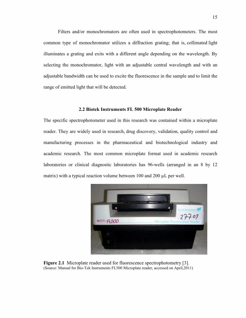
Figure 2.1 Microplate reader used for fluorescence spectrophotometry [3]. (Source: Manual for Bio-Tek Instruments FL500 Microplate reader, accessed on April,2011)
16
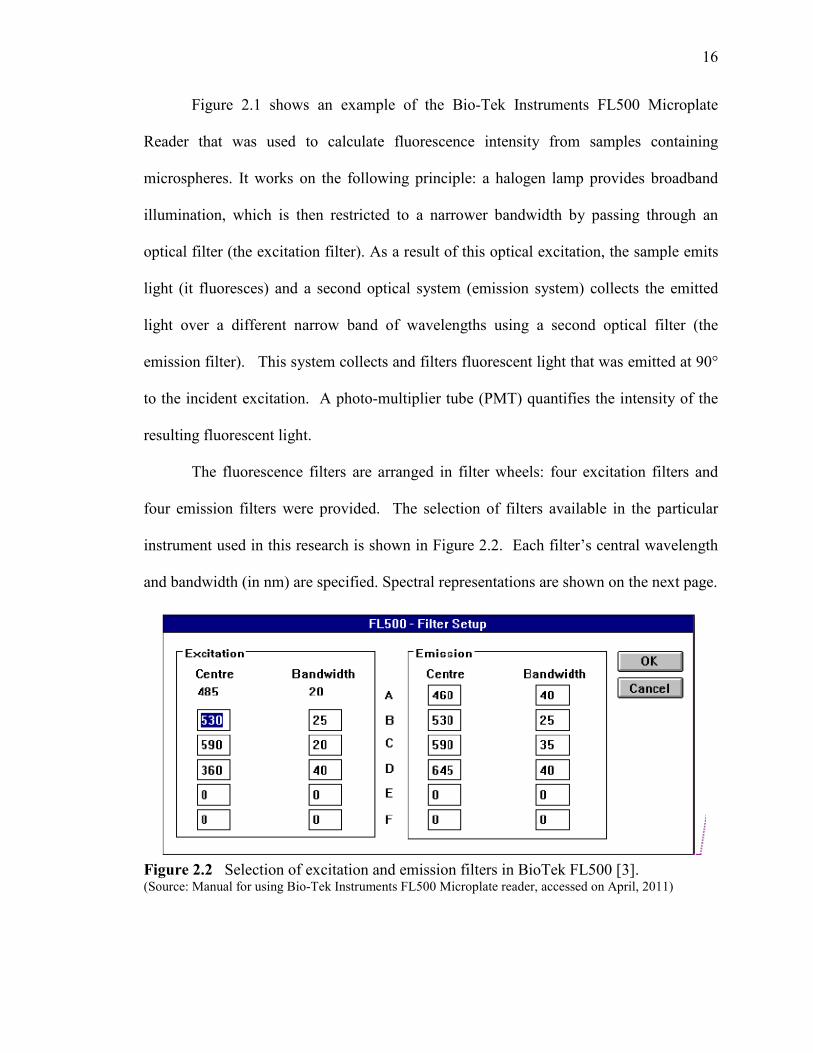
Figure 2.1 shows an example of the Bio-Tek Instruments FL500 Microplate
Reader that was used to calculate fluorescence intensity from samples containing
microspheres. It works on the following principle: a halogen lamp provides broadband
illumination, which is then restricted to a narrower bandwidth by passing through an
optical filter (the excitation filter). As a result of this optical excitation, the sample emits
light (it fluoresces) and a second optical system (emission system) collects the emitted
light over a different narrow band of wavelengths using a second optical filter (the
emission filter). This system collects and filters fluorescent light that was emitted at 90°
to the incident excitation. A photo-multiplier tube (PMT) quantifies the intensity of the
resulting fluorescent light.
The fluorescence filters are arranged in filter wheels: four excitation filters and
four emission filters were provided. The selection of filters available in the particular
instrument used in this research is shown in Figure 2.2. Each filter’s central wavelength
and bandwidth (in nm) are specified. Spectral representations are shown on the next page.
Figure 2.2 Selection of excitation and emission filters in BioTek FL500 [3]. (Source: Manual for using Bio-Tek Instruments FL500 Microplate reader, accessed on April, 2011)

17
Emission Filters
0
0.2
0.4
0.6
0.8
1
400 450 500 550 600 650 700
Wavelength (nm)
Transm
ittance
Figure 2.3 Spectra of emission filters available in the Bio Tek FL500.
Excitation Filters
0
0.2
0.4
0.6
0.8
1
400 450 500 550 600 650 700
Wavelength (nm)
Transm
ittance
Figure 2.4 Spectra of excitation filters available in the Bio Tek FL500.
18
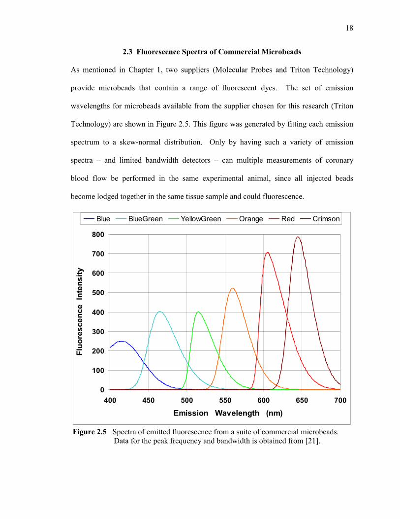
2.3 Fluorescence Spectra of Commercial Microbeads
As mentioned in Chapter 1, two suppliers (Molecular Probes and Triton Technology)
provide microbeads that contain a range of fluorescent dyes. The set of emission
wavelengths for microbeads available from the supplier chosen for this research (Triton
Technology) are shown in Figure 2.5. This figure was generated by fitting each emission
spectrum to a skew-normal distribution. Only by having such a variety of emission
spectra – and limited bandwidth detectors – can multiple measurements of coronary
blood flow be performed in the same experimental animal, since all injected beads
become lodged together in the same tissue sample and could fluorescence.
0
100
200
300
400
500
600
700
800
400 450 500 550 600 650 700
Emission Wavelength (nm)
Fluoresc
ence
Intens
ity
Blue BlueGreen YellowGreen Orange Red Crimson
Figure 2.5 Spectra of emitted fluorescence from a suite of commercial microbeads. Data for the peak frequency and bandwidth is obtained from [21].

19
Additional separation between the fluorescent signals from multiple varieties of
beads embedded in a tissue sample can be obtained by taking advantage of the different
excitation spectra for the fluorescent dyes in the beads. Fluorescence is excited by
photons of higher energy than the photons that are released during fluorescence. By
Planck’s law, these higher energy photons have higher frequency and thus shorter
wavelength. Some photon energies are better able to excite the fluorescent response of
the dye, and this “efficiency” of excitation is expressed as the excitation spectrum for the
fluorescent response. For example, the excitation spectrum and the emission spectrum
for yellow-green fluorescent microbeads is shown in Figure 2.6 The excitation spectrum
–in blue – peaks at a lower wavelength (higher frequency and energy); in this case, the
difference is 10 nm. For the greatest excitation of fluorescence, the excitation should
Figure 2.6 Excitation (blue) and emission (red) spectra for yellow-green dye [33]. (Source: http://probes.invitrogen.com/media/spectra/8811h2o.jpg)

20
occur at wavelengths near this peak. Note that the excitation efficiency falls off quickly
for slightly longer wavelengths, while there is a greater extent of efficient excitation for
wavelengths somewhat shorter than the best wavelength. If the excitation of fluorescence
is to be minimized when assaying for another variety of bead in a tissue sample, then the
exciting wavelengths could be limited by a filter to wavelengths well away from the peak
excitation “efficiency”.
Note that the spectrum of emitted fluorescent light is the same no matter what
wavelength is used to excite the fluorescence [24]. This occurs because the variety of
molecular vibrational modes excited when the dye molecule absorbs photons from a
variety of wavelengths all die out quickly (within 10-14 to 10-10 sec). Thus, the dye
molecule quickly reduces its vibrational energy to a common minimal state before the
fluorescent photon emission event occurs, an event which happens on a much slower time
scale (10-9 to 10-7 sec) [24].
2.4 Choice of Fluorescent Dyes used in Microbeads
The goal of this thesis was to measure coronary flow reserve. Thus, two successive
measurements of coronary flow were required: (1) with the rat at a baseline resting state,
when coronary flow will be minimal, and (2) during infusion of a vasodilator, when the
coronary flow will be maximal. Consequently, microbeads with two different dyes must
be infused, and both varieties will remain simultaneously embedded in the tissue samples
to be assayed by fluorescent spectrophotometry. The particular pair of microbead dyes to
use must be chosen so that their fluorescent signals can be essentially completely

21
separated by a judicious choice of the emission spectra of the dyes themselves and by the
excitation and emission filters available in the spectrophotometer.
Several experimental factors affected the choice of the two microbead dyes.
Firstly, two of the chemical components used in processing the tissue and beads (the
solvent 2-ethoxy-ethyl-acetate and the detergent Tween 80) both possess intrinsic
fluorescent properties themselves, and their fluorescence is emitted in the blue part of the
spectrum. Consequently, microbeads with blue and blue-green dyes were not chosen for
this project. Secondly, photomultiplier tubes are generally less sensitive to longer
wavelengths, so the dye having the longest emission wavelength (crimson) was not
chosen so that the detection system would maintain the best possible sensitivity. The
remaining three dyes were: yellow-green, orange, and red. As Figure 2.5 showed, the
emission spectrum of the orange dye overlapped significantly with both of the other two.
Hence, the orange dye was not chosen.
The two selected microbead dyes were thus (1) yellow-green, and (2) red. Their
emission spectra did not overlap significantly. Moreover, as the next section shows, the
choice of excitation and emission filters made it possible that there was essentially
complete separation between the fluorescent signals that would be measured from the two
beads in the spectrophotometer – even when they both co-existed in the same tissue
sample.

22
2.4 Choice of Excitation and Emission Filters
Table 2.1 (below) reports the filter set chosen to be used when the fluorescence signal
from either of the two chosen microbeads was to be measured. The emission filter best
matched to the yellow-green emission spectrum (Figure 2.5) is the second one from the
left shown in Figure 2.3, which has maximum transmittance at 530 nm. Similarly, the
emission filter best matched to the red emission spectrum is the right-most one shown in
Figure 2.3, which has maximum transmittance at 645 nm. The transmittance spectra from
these two filters do not overlap, which enhances the separation of the fluorescent signals
when both dyes coexist.
The excitation spectrum for yellow-green dyed microbeads was shown in Figure
2.6; 505 nm was the wavelength that most efficiently excited their fluorescence. The
excitation filter that best matched this excitation spectrum was the left-most one shown in
Figure 2.4, which has maximum transmittance at 485 nm. The excitation spectrum for
red dye peaked at 580 nm, so the right-most filter shown there (peak = 590 nm) was
chosen for this case. Note that the spectra from the two excitation filters do not overlap,
which – just as in the case for the emission filters – further enhances the separation of
fluorescent signals.
Table 2.1 Filters providing best match to excitation and emission spectra
Fluorescent Color
Wavelength at Peak Emission
(nm)
Emission Filter Center of
Transmittance (nm)
Wavelength for Best Excitation
(nm)
Excitation Filter Center of
Transmittance (nm)
Yellow - Green 515 530 505 485
Red 605 645 580 590

23
2.6 Determination of Calibration Curve
As explained in Chapter 1, the number of microbeads trapped in a tissue sample is the
key measure used in the tracer method to determine coronary blood flow. The
fluorescent intensity of a tissue sample containing embedded microbeads provides a
measure proportional to the number of microbeads contained in that sample. However,
both the proportionality constant and any offset must be determined by a calibration
procedure before the fluorescent signal can be related quantitatively to the number of
microbeads.
Calibration requires measuring the fluorescence of solutions containing known
numbers of microbeads. The most difficult part here is developing a reliable procedure
that will accurately set the number of microbeads in a solution. The starting point for this
procedure is the known concentration of microbeads in the stock solution of microbeads
provided by the supplier. The microbeads we used were packaged in a solution
containing 1 million microspheres per milliliter. By accurately diluting this stock
solution, and by accurately measuring out known volumes of these dilute solutions, a
variety of samples containing known numbers of microbeads were prepared.
The number of microbeads in the calibration samples should span the range
anticipated to occur in the tissue samples. A large number of microbeads would be on the
order of 10,000 to 20,000. The minimum number of microbeads that provides a reliable
statistical estimate is on the order of 400. Calibration standards spanning this range were
prepared.
Appendix I provides the detailed steps in the procedure used to prepare the
calibration standards. Briefly, the first step was to prepare a 10:1 diluted solution of
24
microbeads. This solution would thus have 100,000 microbeads per milliliter. Since the
sample size used in the wells of the 96-well plate is 100 µl, a sample drawn from this
solution would contain 10,000 microbeads. This is the maximum number that was used
in a calibration standard. Subsequent 2:1 dilutions then produced standards containing:
5000, 2500, 1250, 625, and 312 microbeads. These standards spanned the range over
which calibration was performed.
During the dilution and sample loading procedure, extreme care was taken to
maintain the microspheres in solution and to prevent clumping and aggregation of
microspheres. A small amount of detergent (Tween 80) was used in the diluting solutions
to minimize clumping and aggregation, and solutions were often agitated vigorously in a
vortex mixer.
Accurate measurement of solution volumes was also required. This was
accomplished using well-calibrated mechanical pipettes, which are common in
biochemical laboratories. Following the proper pipetting procedure was also important.
2.7 Results of Calibration Curves
Five replicate determinations of a calibration curve were performed for each of
the two varieties of microbeads used in this study. Table 2.2 and Figure 2.7 provide
typical results for one such calibration curve, which was performed on solutions
containing yellow-green microspheres. Appendix II provides similar detailed results for
all of the 10 calibration curves. Each calibration curve maintained a tight linear relation
between microbead number and fluorescence intensity. The R2 values for linear
regression were all above 0.9936, and most were above 0.9990.

25
Table 2.2 Typical calibration measurements for yellow – green microspheres Number
Of Microspheres
Fluorescent Intensity
(arbitrary units)
10,000 8683
5,000 4288
2,500 2100
1,250 1001
625 528
312 300
Figure 2.7 Typical calibration regression line for yellow-green microspheres

26
However, the replications of the calibration curves did not all produce slopes of
the regression lines that were in close agreement with one another (see Figures 2.8 and
2.9). Since each individual regression line was rather linear without much scatter, it
seemed likely that the major contribution to the disagreement among regression lines
arose due to experimental uncertainty in the first step of the calibration procedure. The
stock solution may not have been sufficiently well-mixed when the sample was
withdrawn, or there may have been some error in withdrawing a 1 ml volume into a
plastic syringe, since a calibrated pipette could not perform this step.
2.8 Averaging calibration curves
To overcome the uncertainty in the regression coefficient, the results from the 5 replicate
calibration curves were averaged together for each variety of microbead. Averaging was
thought to reduce the uncertainty introduced during the initial microbead withdrawal
from the stock solution. Tables 2.3 and 2.4 on the next pages report the averaging
process. Each averaged relationship then became the standard calibration curve for that
color microsphere, which was used to convert the fluorescence from a tissue sample into
the number of microspheres contained within that sample.
The final calibration curves were:
For yellow green microspheres: If = 0.9256 Ns - 4.9102
For red microspheres: If = 1.0954 Ns + 0.8414
where If is the fluorescent intensity and Ns is the number of microspheres.
Note that red microspheres produced slightly more fluorescence intensity per sphere.
The offset values were not statistically different from zero.

27
Calibration of Yellow-Green Microspheres
Table 2.3 Summary of calibration for yellow – green microspheres
Trial Number Slope of
Regression
Intercept of
Regression
R-squared
1 1.1455 + 4.4194 0.9992
2 0.9229 -92.562 0.9992
3 0.8696 -36.541 0.9998
4 0.9188 -30.379 0.9976
5 0.774 +130.56 0.9974
AVERAGE 0.9256 -4.9102
Yellow-Green Calibration Curves
0
5000
10000
0 5000 10000
Number of Microspheres
Fluorescen
t Intensity
Test 1 Test 2 Test 3 Test 4 Test 5 Average
Figure 2.8 Linear regression calibration curves for yellow – green microspheres
28
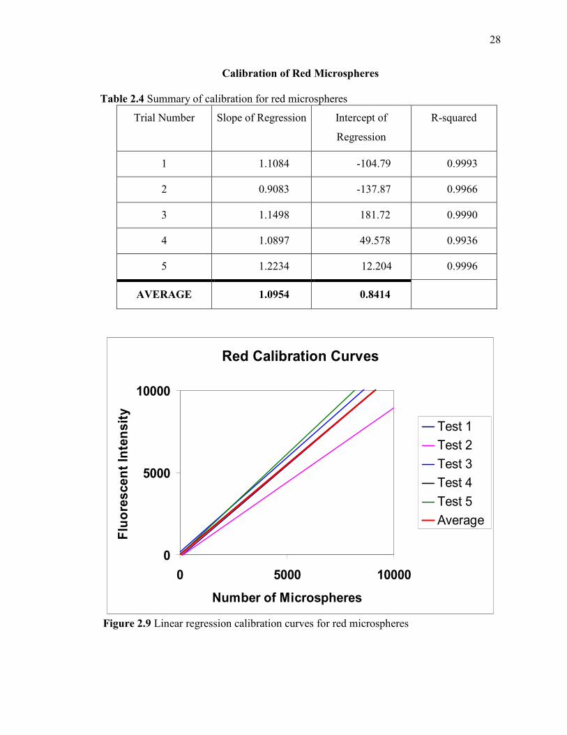
Calibration of Red Microspheres
Table 2.4 Summary of calibration for red microspheres
Trial Number Slope of Regression Intercept of
Regression
R-squared
1 1.1084 -104.79 0.9993
2 0.9083 -137.87 0.9966
3 1.1498 181.72 0.9990
4 1.0897 49.578 0.9936
5 1.2234 12.204 0.9996
AVERAGE 1.0954 0.8414
Red Calibration Curves
0
5000
10000
0 5000 10000
Number of Microspheres
Fluoresc
ent Intensity
Test 1 Test 2 Test 3 Test 4 Test 5 Average
Figure 2.9 Linear regression calibration curves for red microspheres
29
CHAPTER 3
EXPERIMENTAL TECHNIQUES TO DETERMINE CORONARY BLOOD
FLOW IN RAT ANIMAL MODEL
When appropriately sized microspheres are used, regional blood flow is proportional to
the number of microspheres trapped in the organ of interest.
3.1 Source of Fluorescent Microspheres
Triton Technology (San Diego, CA) and Molecular Probes (Eugene, OR) are the two
major companies manufacturing fluorescent microspheres used in biomedical research
and various other applications. For our procedures we have used fluorescent
microspheres sold by Triton Technology. Triton Technology sells two types of
fluorescent microspheres: Triton Technology Dye-Trak 'F' fluorescent microspheres and
the FluoSpheres® manufactured by Molecular Probes. We have used Molecular Probes
Fluospheres (with Triton Technology packaging) for our experiments. Fluospheres are
non-radioactive fluorescent microspheres for high sensitivity measurement of regional
blood flow quantified by spectrofluorometry. Each 20 ml bottle contains 20 million
spheres, 15 µm in diameter, in a saline solution, with 0.05% Tween 20 as a detergent to
help maintain the microspheres dispersed in solution and 0.02% Thimerosal as a
bacteriostat.
30
3.2 Calculation of Number of Microspheres for Injection A minimum of 400 – 500 microspheres are needed per tissue piece to be 95 % confident
that flow measurement is within 10% of the true value [39]. For regional blood flow
measurements, the total number of microspheres to be injected into the whole animal
must be calculated to assure that a sufficient number reach the particular organ of
interest.
The following equation estimates the minimum total number of microspheres
needed per injection [39]:
Nmin = 400 (n) * [ Qtotal / Qorgan ] (3.1)
Where, Nmin = minimum total number of microspheres needed for injection
n = total number of organ pieces in the organ with the smallest blood flow
Qorgan = total blood flow through an organ of interest with the smallest blood flow
Qtotal = cardiac output
Applying this equation to our procedure, we first must estimate the cardiac output
expected in the experimental animals we used. The cardiac index observed in Sprague
Dawley rats of the same age and weight as we used is approximately 350 ml/min/kg [22].
Considering the approximate weight of the rats we used to be 400g,
Cardiac Output = Cardiac Index * Mass of an animal
= (350 * 400) / 1000
= 140 ml/min
Since our organ of interest is the heart, which has a relatively large blood flow, the
“organ” with the smallest blood flow will actually be the “virtual organ” created by the
reference withdrawal of blood. Since we will withdraw the reference blood flow at a rate
31
of 0.5 ml/min, the estimate of the minimum total number of microspheres needed per
injection is:
Nmin = 400 (n) * [Qtotal / Qorgan ]
= 400 (1) * [140 / 0.5]
= 112,000
Where, n = number of organ pieces = reference blood flow sample = 1
Qorgan = reference blood flow = 0.5 ml/min
Qtotal = Cardiac output = 140 ml/min
Thus, a minimum of 112,000 microspheres per injection was needed for our
procedure. We have injected 0.5 ml volume of microsphere solution, which contains
500,000 microspheres. Thus, the volume used for our procedure was quite enough to trap
a sufficient number of microspheres in the tissue and blood samples. Usually double the
minimum number of microspheres are injected to make sure that low flow organ pieces
have an adequate number of microspheres [39]. Our procedure met this guideline as
well.
3.3 Preparation of fluorescent microspheres for injection
Aggregation is a major problem associated with fluorescent microspheres. This might
clog a blood vessel, resulting in damage which might result in the death of an animal.
Aggregation of the particles is prevented by the use of small amounts of detergent in the
injectate, or by suspending them in a solution containing macromolecules. A detergent
named Tween 80 is normally added to the solution to prevent aggregation and clumping
together of microspheres. However, the concentration of the detergent cannot be too high,
otherwise it could damage the lipids in the cell membranes of endothelial cells or blood
32
cells. Therefore, we used a concentration of 250 µl. During the microsphere injection
procedure, special care is taken of in order to avoid aggregation of microspheres.
Method: 1) Remove the bottle from the refrigerator and check supernatant solution. Ideally, the solution should stay clear due to the presence of thimerosal in it. Thimerosal is a bacteriostat which prevents the growth of any bacteria or fungi thus preventing cloudy fluid and contamination. 2) Vortex the bottle vigorously for 5 – 15 seconds using a vortex mixer. Vortexing ensures proper mixing of the solution thus preventing aggregation of microspheres. 3) Place the bottle in an ultrasonic water bath for at least 30 minutes to allow dispersion of microspheres. This allows proper mixing of microspheres with the liquid solution. Be careful with the sonication time as the heat generated might melt the microspheres. 4) Continue to sonicate the microspheres until the sample is used for the procedure. 5) Just prior to injection, vortex the vial of microspheres again and withdraw the desired volume of 0.5 ml immediately. The injected volume drawn into syringe should then be injected immediately into the body of animal. If injection time is delayed, vortex the microspheres thoroughly again. 6) Injection time varies for each procedure and should be determined prior to injection. Injection to left heart takes a short time (normally 5 – 15 seconds). In our procedure, injection time is 5 seconds. 7) Slow and steady injections allow for proper mixing of microspheres with the blood in the left ventricle. 8) After injection, flush the dead space of the catheter thoroughly with saline and change the stopcock to avoid contamination of subsequent injections.
3.4 Reference blood flow sampling
A reference blood flow sample allows calculation of regional flow in ml / min. The
catheter used for the withdrawal of sample should be accurately positioned so that a
blood sample containing well mixed microspheres can be obtained. Blood samples should
33
be obtained as close to the organ of interest as possible without interfering too much with
the normal blood flow. The reference withdrawal pump must be accurately calibrated at
0.5 (ml/min) so that reference blood is withdrawn at a uniform preset rate for a period of
2 minutes. Although glass syringes and containers would have been preferred as they
decrease microsphere loss by avoiding adhesion to walls, which could occur in case of
plastic syringes or containers, we found that use of plastic syringes was adequate and did
not result in loss of microspheres.
Researchers say that 15% of blood volume is the maximum that can be taken out
at a stretch from the body, say during donation of blood. More than 15% results in a
significant loss of arterial pressure and might result in some heart problems.
Since the animals used in our procedure weigh 350-450g, withdrawal of minimum
reference blood should be calculated. For a rat weighing 350g, blood mass = 8% of body
mass = (0.08)(350g) = 28 g. This equates to approximately 28 ml of blood since the
density of blood is only slightly greater than that of water.
If 2 ml is withdrawn as reference blood during microsphere procedure, then it
accounts for 7% loss of blood from the body which is quite tolerable and should not
create a bad impact on the condition of the animal.
Similarly, for a rat weighing 450g, its blood volume is estimated to be 36 ml. If 2
ml is withdrawn as reference blood during microsphere procedure, then it accounts for
5% loss of blood from the body of animal which is tolerable and does not affect the
condition of animal.

34
Therefore, withdrawal of 0.5 (ml/ min) for a period of 2 minutes results in 5% -
7% of blood loss which is preferred for our procedure to avoid excessive loss of blood in
an animal.
3.5 Animals
Male Sprague Dawley rats, body weight 350 – 450 g, age 8 - 12 weeks, were housed in
separate cages and maintained in a temperature regulated environment. The animals were
used as described in a protocol approved by IACUC committee (Institutional Animal
Care and Use Committee) of UMDNJ – Newark. This institution is accreditated by
AAALAC (Association for Assessment and Accreditation of Laboratory Animal Care)
International program. Two animals were used. Both were subjected to injections of
Triton Technology 15 µm diameter fluorescent microspheres of two different colors:
yellow-green microspheres used for baseline measurements and red microspheres used
for measurements after infusion with adenosine.
3.6 Surgery
Surgery was performed by an experienced doctoral student, Xin Zhao, in the department
of Cell Biology and Molecular Medicine at UMDNJ – Newark, trained to perform
cardiovascular surgery on rats. An anesthetic technique that has minimal effect on the
heart rate is essential. The following anesthetic regime resulted in heart rates that were
close or slightly below the rate for an alert, resting rat and allowed excellent animal
recovery. Anesthesia was induced with a mixture of ketamine (70mg/ kg) and xylazine
(7mg/ kg) administered intramuscularly. Since the experimental procedure was not for a
35
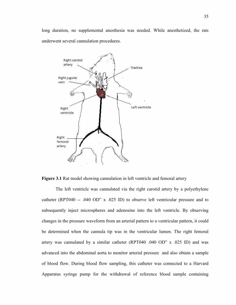
long duration, no supplemental anesthesia was needed. While anesthetized, the rats
underwent several cannulation procedures.
Figure 3.1 Rat model showing cannulation in left ventricle and femoral artery
The left ventricle was cannulated via the right carotid artery by a polyethylene
catheter (RPT040 -- .040 OD” x .025 ID) to observe left ventricular pressure and to
subsequently inject microspheres and adenosine into the left ventricle. By observing
changes in the pressure waveform from an arterial pattern to a ventricular pattern, it could
be determined when the cannula tip was in the ventricular lumen. The right femoral
artery was cannulated by a similar catheter (RPT040 .040 OD” x .025 ID) and was
advanced into the abdominal aorta to monitor arterial pressure and also obtain a sample
of blood flow. During blood flow sampling, this catheter was connected to a Harvard
Apparatus syringe pump for the withdrawal of reference blood sample containing
36
microspheres that are adequately mixed. Right jugular vein was cannulated by MRE 040
.40OD" X .025 ID catheter for the injection of saline to restore blood volume after each
microsphere injection and sampling procedure.
The entire procedure takes about 1.5 – 2 hours. The animals were then allowed
to recover for 2-3 hours after the completion of cannulation surgery. After the normal
hemodynamic condition of the animal was recovered, a subsequent microsphere injection
procedure could be performed.
3.7 Procedure for Injection of Microspheres
Systemic hemodynamic and regional blood flow was determined using 15 micrometer
diameter fluorescent microspheres (FluoSpheres® Triton Technology, San Diego, CA,
USA (20 million 15 micron spheres per 20 ml vial)). Briefly, two different colors of
fluorescent microspheres were used. The colors of microspheres were selected as
previously described to avoid spillover between the colors. Yellow-green and red colors
have been selected for our experiment. Yellow-green microspheres are used for baseline
measurement and red microspheres are used for measurements after infusion with
adenosine.
The procedure is as follows: 1) Shake well the bottle containing microspheres of desired color and place it in an ultrasonicator. This allows proper mixing of microspheres and prevents aggregation of microspheres. 2) The bottle containing microspheres are sonicated until the desired amount is removed and without wasting any time, the microspheres are injected directly into the body of animal. 3) Two Harvard apparatus infusion pumps were used for procedure: One pump is used for the injection of adenosine at the rate of 0.15 (mg/kg/min), second pump is used for the
37
withdrawal of reference blood sample at the rate of 0.5 (ml/min) for a period of 2 minutes.
4) Four 1cc plastic syringes were used in infusion pumps: two syringes were used for collecting blood and the remaining two were used for injection of microspheres. Heparin coated syringes were used for the collection of blood samples to avoid the clot of blood once it is collected in a syringe. Also, once collected in heparin coated syringe, it then becomes easy to transfer in any other container without any clot observed. 5) The diameter for the syringe was set to 4.78 mm. 6) The withdrawal pump was calibrated at the predetermined withdrawal rate, including the catheters, extension tubing and syringes that would be used for the reference withdrawal. 7) The syringes would be connected to the withdrawal pump to the catheters and the extension tubing so that everything is set up for withdrawing the reference blood sample. The stopcock is turned off to avoid clotting of blood into the catheter dead space until injection. 8) Four paper pins were placed, one at each corner of surgical board, that hold each limb of the animal. Horizontal distance between the pins is 15cm. Vertical distance between the pins is 12cm. 9) Core temperature of the animal was monitored with a rectal probe and maintained at 36.5 degree Celsius with an automatic heating lamp. 10) The hemodynamics of the rat is checked for its normal condition before the injection of microspheres. 11) Yellow-green microspheres are injected first into the body of animal to determine baseline measurements and then red microspheres are injected to determine measurements after infusion of adenosine. 12) Once the microspheres had been drawn into the injection syringe, the withdrawal pump was started and made sure that the flow was smooth without any clot. 13) Now, a volume of 0.5 ml of yellow green fluorescent microspheres was injected over a period of 5 seconds followed by the flush of saline. 14) Simultaneously, the reference blood sample was withdrawn for a total interval of 2 minutes, 1 minute each for both the color of microspheres. At the end of the withdrawal, the pump was turned off, the stopcocks were opened and the blood remaining in the extension tubing was drawn into the syringe.

38
15) The reference blood was then transferred from heparinized syringe into polypropylene tubes for further processing. Also, the syringes and the extension tubing were washed with 2% Tween 80 and this solution was then added to the blood samples to avoid any loss. 16) Adenosine which works as a potent dilator of arterioles was then infused into the left ventricle via the catheter in the left ventricle. 17) After the rat’s hemodynamic state had stabilized under the adenosine infusion, 0.5 ml volume of red microspheres was injected over a period of 5 seconds followed by the flush of saline. 18) The reference blood sample was collected in heparinized syringe which is then transferred to polypropylene tubes for further processing.
This injection procedure produced two sets of microspheres in each rat. At the end
of the procedure, the rats were euthanized with an overdose of anesthetic. The heart was
removed, weighed and placed in a polypropylene tube. The reference blood sample and
heart tissue were then digested by 2.3 M ethanolic KOH and 0.25 % Tween 80 for a
period of 48 hours. At the end of digestion, microspheres were recovered by the
sedimentation method and the microsphere dye was extracted by using 3 ml of 2-
ethoxyethyl acetate, that dissolved the plastic spheres and so released the fluorescent dye
into solution.

39
CHAPTER 4
EXPERIMENTAL TECHNIQUES TO RECOVER MICROSPHERES
FROM TISSUE AND BLOOD
4.1 Three Alternative Methods to Separate Microspheres From Tissues
Microspheres must be physically separated from the tissue or blood in order to quantify
the number of microspheres in each sample.
There are three practical methods to recover microspheres from digested tissues
[39]:
1) Negative pressure filtration
2) Polyamide woven filtration devices (manufactured by Perkin Elmer)
3) Sedimentation
All three methods will be described below, along with the disadvantages of both
the filtration methods. Ultimately, the sedimentation method was the one chosen for use
in this research. The details of the sedimentation method will be presented in other
sections in this chapter. The initial key step in all three procedures is digestion of tissue
or blood sample. All methods use ethanolic KOH, a very powerful digesting solution.
4.2 Negative Pressure Filtration
In the case of the negative pressure filtration technique, the volumes and concentrations
of solutions are not critical. Negative pressure filtration works on digested heparinized
blood samples and solid tissue. After the samples have been digested with KOH, the
microspheres are physically separated by negative pressure filtration. Filtration is usually
40
performed with a combination of a Poretics filtration device using Poretics polycarbonate
filters [39].
Disadvantages:
1) Digested tissue samples should not stand unfiltered for a long period of time since the fat in them may solidify and this may result in damage to the sample. 2) The method is labor intensive. 3) There may be microsphere loss when the tissue sample is transferred from one vessel to another or if the filter fails to trap all microspheres. 4) The filters must be changed every time for each new sample. This may increase the expense. 5) The filtration process may proceed slowly as the filter might become clogged with microspheres or tissue debris.
4.3 Polyamide Woven Filtration Devices
These devices are specifically made to isolate fluorescent microspheres from CPD
(citrate phosphate dextrose) anticoagulated blood or digested tissues [39]. Each tissue
sample is digested, filtered and the fluorescent dyes are extracted in a single container.
The devices are polypropylene and consist of three stages. Digestion is done with
ethanolic KOH.
Disadvantages:
1) These devices offer limitations with heparin containing blood samples. 2) There may be microsphere loss when the tissue sample is transferred from one vessel to another or if the filter fails to trap all microspheres. 3) Digestive tissue samples should not stand unfiltered for a long period of time since the fat in them may solidify and may result in damage to the sample. 4) Filters need to be changed after every microsphere procedure.

41
4.4 Sedimentation
Sedimentation is the tendency for particles in suspension to settle out of the fluid in
which they are entrained, and come to rest against a barrier. This is due to their motion
through the fluid in response to the forces (gravitational force or centrifugal force or
electromagnetic force) acting on them.
Sedimentation of microspheres based on centrifugal force (as in a centrifuge) is
possible if the specific gravity of the solution is less than that of microspheres.
Microspheres have a density of 1.05 g / ml, which is close to the density of red blood
cells and myocardial tissue. Ethanolic KOH has a density on the order of 0.8 g / ml,
which is much smaller compared to that of microspheres.
Sedimentation is a 7 day procedure. It is the most effective procedure and also it
is cost effective. The chemical solutions can be easily prepared in the laboratory, and the
polypropylene tubes used for the procedure are inexpensive and available in bulk. The
steps in the procedure are summarized in Figure 4.1 After digesting the tissue with
ethanolic KOH, the procedure consists of 3 successive stages of centrifugation
interspersed by washes with specific solutions or buffers. As a final step, a chemical is
added (2-ethoxy-ethyl-acetate) that dissolves the plastic microspheres and thus releases
the fluorescent dye into solution. A final centrifugation (not shown in Figure 4.1)
separates this solution from the remnants of the plastic microspheres. A sample of this
final supernatant is then subjected to fluorometry to determine the number of
microspheres.
42
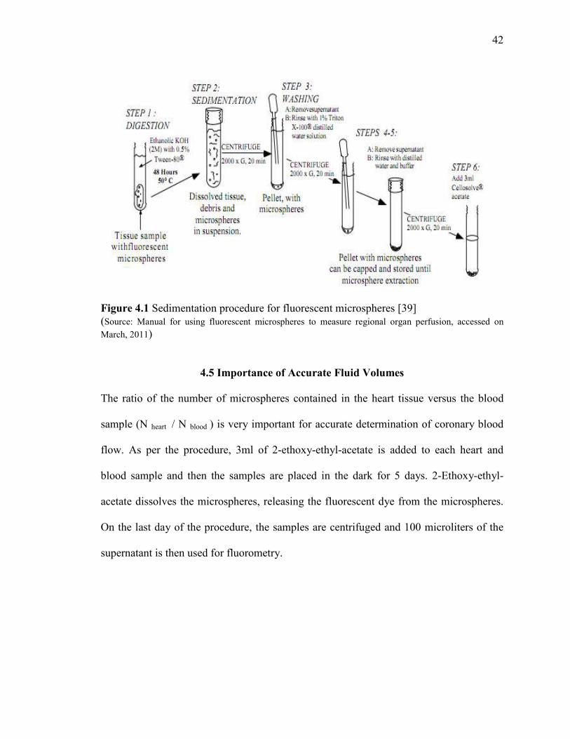
Figure 4.1 Sedimentation procedure for fluorescent microspheres [39] (Source: Manual for using fluorescent microspheres to measure regional organ perfusion, accessed on March, 2011)
4.5 Importance of Accurate Fluid Volumes
The ratio of the number of microspheres contained in the heart tissue versus the blood
sample (N heart / N blood ) is very important for accurate determination of coronary blood
flow. As per the procedure, 3ml of 2-ethoxy-ethyl-acetate is added to each heart and
blood sample and then the samples are placed in the dark for 5 days. 2-Ethoxy-ethyl-
acetate dissolves the microspheres, releasing the fluorescent dye from the microspheres.
On the last day of the procedure, the samples are centrifuged and 100 microliters of the
supernatant is then used for fluorometry.
43
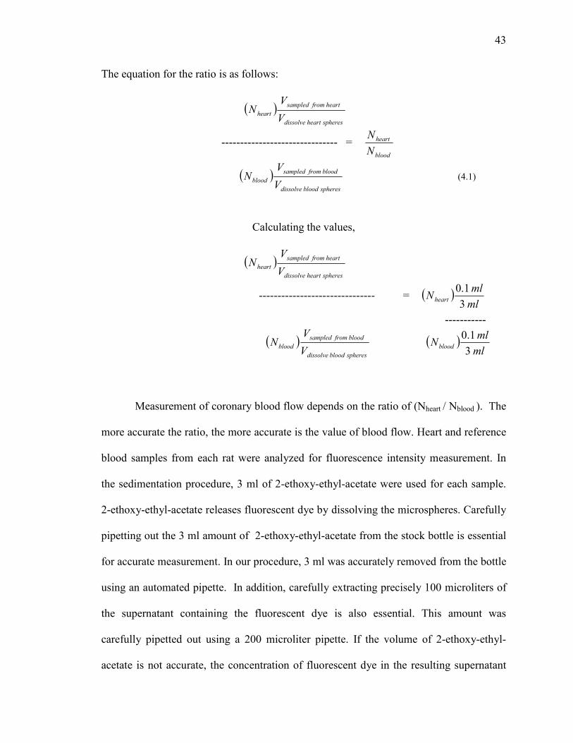
The equation for the ratio is as follows:
( )spheresheartdissolve
heartfromsampledheart V
VN
------------------------------- = blood
heart
NN
( )spheresblooddissolve
bloodfromsampledblood V
VN (4.1)
Calculating the values,
( )spheresheartdissolve
heartfromsampledheart V
VN
------------------------------- = ( )mlml
Nheart 31.0
-----------
( )spheresblooddissolve
bloodfromsampledblood V
VN ( )
mlml
Nblood 31.0
Measurement of coronary blood flow depends on the ratio of (Nheart / Nblood ). The
more accurate the ratio, the more accurate is the value of blood flow. Heart and reference
blood samples from each rat were analyzed for fluorescence intensity measurement. In
the sedimentation procedure, 3 ml of 2-ethoxy-ethyl-acetate were used for each sample.
2-ethoxy-ethyl-acetate releases fluorescent dye by dissolving the microspheres. Carefully
pipetting out the 3 ml amount of 2-ethoxy-ethyl-acetate from the stock bottle is essential
for accurate measurement. In our procedure, 3 ml was accurately removed from the bottle
using an automated pipette. In addition, carefully extracting precisely 100 microliters of
the supernatant containing the fluorescent dye is also essential. This amount was
carefully pipetted out using a 200 microliter pipette. If the volume of 2-ethoxy-ethyl-
acetate is not accurate, the concentration of fluorescent dye in the resulting supernatant
44
could vary, which would vary the number of microspheres obtained when 100 microliters
of the supernatant is extracted for measurement. Similarly, the volume of supernatant
must be reproducibly pipetted out, so that the ratio of the number of microspheres is the
same as the ratio of dye concentrations in the supernatant fluids form tissue and blood
samples.
4.6 Solutions Used in the Sedimentation Method
The six different solutions used throughout the sedimentation procedure are as follows:
1) 2.3 M Ethanolic KOH with 0.5 % Tween 80
100 ml of ethanol is added to the glass beaker containing a mixture of 3 gm KOH
and 0.5 gm Tween 80. The solution is stirred continuously for approximately 20 minutes
until a clear solution is obtained. Tween 80, a viscous and water soluble yellow fluid, is
used as an emulsifier. KOH, since it is obtained in pellet form, needs to be stirred
properly to ensure proper mixing. Freshly made KOH solution, warm due to the
exothermic reaction, aids in tissue digestion.
2) Internal standard ( This is optional )
The microspheres are vortexed and sonicated for 30 seconds and then 1ml of solution is
immediately withdrawn using a sterile syringe. This 1ml of solution is added to 100 ml of
0.25% Tween 80. A magnetic stirrer is used to stir the solution continuously until its use.
3) 1% Triton X-100
10 grams of Triton X-100 is added to 1 liter of distilled water and stirred until in solution.
45
4) Distilled water phosphate buffer
5.88 grams of monobasic KH2PO4 is added to 200 ml distilled water. 22.9 grams of
dibasic KH2PO4 is added to 800 ml distilled water. The two solutions are then mixed
together. 28.6 ml of this combined solution is added to 1000 ml of distilled water and
stirred until they mix really well. This produces a distilled water phosphate buffer, which
is a solution used for rinsing.
5) 0.25 % Tween 80
2.5 grams of Tween 80 is added to 1 liter of distilled water and stirred continuously with
a magnetic stirrer until in use.
6) 2 – Ethoxy-ethyl-acetate ( also known as Cellosolve acetate )
This is a solution used to dissolve microspheres and release dye. 2–ethoxy-ethyl-acetate
should not be confused with ethyl cellosolve, since that doesn’t dissolve the
microspheres.
4.7 Calculation of Centrifuge Rotation Rate
During the sedimentation method, a centrifugal acceleration equivalent to 2000 times the
acceleration of gravity (i.e., 2000Gs) had to be achieved. The faster the centrifuge rotates,
and the longer the radial distance to the sample being centrifuged, the stronger the
centrifugal acceleration. The calculations below were performed to determine the rotation
rate required to achieve 2000Gs for the specific centrifuge and sample tubes that were
used in this research.
46
A centrifuge is a laboratory instrument driven by electric motor that puts an object
in rotation around a fixed axis and thus induceses a centrifugal force perpendicular to the
axis. The centrifugal acceleration generated by the instrument is such that it causes more
dense substances to separate out along the radial direction at the bottom of the tube. The
centrifuge consists of rotating units, called the rotor, which has its own specifications.
We used a Beckman Coulter 366802 – Allegra 6 Benchtop Centrifuge for our
procedure. The centrifuge consists of GH–3.8 / GH–3.8A rotors which have the
following specifications: 1) minimum radius = 86mm; 2) maximum radius = 204mm;
3) maximum allowable rotation rate = 3750 rpm.
During circular motion, the centrifugal acceleration is the product of the radius
and the square of the angular velocity. The acceleration is generally measured in terms of
“G”, which is also called the relative centrifugal force. One “G” is equal to the
acceleration due to gravity at the earth’s surface, which equals 9.8 m/s2 .
In the Beckman centrifuge that we used, the radius to the bottom of the centrifuge
tube (where the denser sample will collect) was measured. We set the rotor to the
minimum distance from the axis of the centrifuge. The radius to the edge of rotor thus
was 8.6 cm. The polypropylene 15 ml centrifuge tubes that we used extended 10 cm
beyond the rotor. Thus, the total radial length to the sample ( r ) = 18.6 cm.
In our procedure, we desired to create an acceleration of 2000 G’s. The angular
velocity ( ω ) required to produce this acceleration ( A ) was calculated as follows:
A = ω2 r
2000 (9.8 m/s2) = ω2 (0.186 m)
ω = 324.6 rad / sec

47
Angular velocity converts to rotational frequency according to the following formula:
ω = 2πf
Thus, the required rotational frequency f = 51.7 rotations/sec, which is 3100 rpm. This
rotation rate is within the range of rotation rates allowed by the manufacturer’s
specifications.
4.8 Details of Sedimentation Procedure
The procedure takes a total of 8 days. The animal was euthanized on the same day soon
after the microsphere injection procedure. The heart was removed, and the left ventricle
was separated from the rest of the heart for recovery of fluorescent microspheres.
Polypropylene 15 ml centrifuge tubes with tightly fitting caps were used.
Day 1
1) The tubes fitted with their caps and the tissue and blood samples were weighed. Each cap should be paired with its tube so that the weight of the capped tube is reliable. 2) 8 ml of ethanolic KOH was then added. Ethanolic KOH should be carefully poured into the tubes since outside spillage can remove writing on the tubes. Also, ethanolic KOH is extremely caustic in nature and can cause burns on skin. 3) The solution was vortexed for a period of 20 seconds. 4) The tubes were then incubated for a period of 48 hours at 50 degrees centigrade at a speed of 150 revolutions per minute. Day 2
Each sample was removed from the incubator and vortexed for 20 seconds per tube. The
samples were then placed back into the incubator to continue for another 24 hours.

48
Day 3
1) Each sample was removed from the incubator and vortexed for about 30 seconds until the particles were re-suspended. Just before the next step, each sample was vortexed again for 5 more seconds. 2) The samples were centrifuged at 3100 rpm for about 20 minutes. 3) All but 1.5 ml of supernatant fluid was removed using a Pasteur pipette attached to suction with a trap. This supernatant was discarded. 4) Approximately 8 ml of 1% Triton X-100 solution was added to each sample, and then each sample was vortexed for about 30 seconds. 5) The samples were centrifuged at 3100 rpm for about 20 minutes. 6) All but 1.5 ml of supernatant fluid was removed using a Pasteur pipette attached to suction with a trap, and the supernatant was discarded. Suction was done carefully to avoid loss of microspheres. 7) 7 ml of distilled of distilled water phosphate buffer was added to each tube, and each tube was vortexed for about 30 seconds until all particles were suspended in the solution. 8) The samples were centrifuged at 3100 rpm for about 20 minutes. 9) All but 1.5 ml of supernatant fluid was removed using a Pasteur pipette attached to suction with a trap, and the supernatant was discarded. 10) Exactly 3 ml of 2-ethoxy-ethyl-acetate was then added to each sample, and each was vortexed for about 30 seconds until the particles were well suspended in the solution. 11) The samples were then placed in a dark room away from light for 5 days.
Day 5
The samples were taken out from the dark room and vortexed for about 20 seconds each
until the pellet broke up.
Day 8
1) The samples were removed from the dark room and vortexed vigorously for about 30 seconds each until the pellet broke up. 2) The samples were centrifuged at 3100 rpm for about 20 minutes.

49
3) Exactly 100 µL of supernatant fluid containing the dye released from the microspheres was then used for fluorometry. 4) The blood and tissue samples were then measured for fluorescence on the same day.
4.9 Advantages of the Sedimentation Method
1) Polypropylene 15 ml centrifuge tubes are used, which are available in bulk in a routine chemistry lab. 2) The tubes are inexpensive as compared to the filters. 3) The procedure although time consuming, is not labor intensive. 4) There is minimal loss of fluorescent microspheres, since they do not have to be transferred from one vessel to another. 5) The sedimentation procedure starts on the same day soon after the microsphere injection procedure. Consequently, there are no issues of digested tissues being left untreated.
50
CHAPTER 5
INITIAL MEASUREMENTS
OF CORONARY BLOOD FLOW AND CORONARY RESERVE IN RATS
USING FLUORESCENT MICROSPHERES
5.1 Summary of Experimental Protocol
Two male Sprague-Dawley rats, body weight 414 and 395 g, both age 12 weeks, were
used for the microsphere injection procedure, as described in detail in Chapter 3. Briefly,
each rat was cannulated with multiple catheters under a mixture of ketamine and xylazine
anesthesia administered intramuscularly. One catheter was introduced through the right
carotid artery into the left ventricle for injection of fluorescent microspheres and
adenosine. The second catheter was introduced through the right femoral artery and
advanced into the abdominal aorta for collection of the reference blood sample during
injection of fluorescent microspheres into the circulation of the rat. The third catheter was
introduced into the right jugular vein for infusion of saline following the withdrawal of
each reference blood sample. After the 1.5 – 2 hour cannulation procedure, the rat was
allowed to recover back to its normal hemodynamic condition.
Soon after the recovery, the rat was subjected to the microsphere injection
procedure. Normal hemodynamic conditions were mandatory before proceeding with the
microsphere procedure. Microspheres which fluoresced at two different colors were used
for the procedure: (1) yellow-green microspheres were used for baseline measurements,
and (2) red microspheres were used for measurements of coronary reserve made during
infusion of a vasodilator (adenosine). During both microsphere injections, reference
blood containing a sample of the injected microspheres was collected at a preset rate of
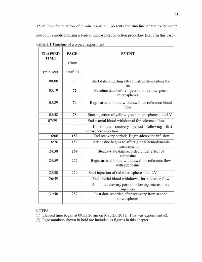
51
0.5 ml/min for duration of 2 min. Table 5.1 presents the timeline of the experimental
procedures applied during a typical microsphere injection procedure (Rat 2 in this case).
Table 5.1 Timeline of a typical experiment
ELAPSED TIME
(min:sec)
PAGE
(from
datafile)
EVENT
00:00 1 Start data recording after finish instrumenting the rat
05:19 72 Baseline data before injection of yellow-green microspheres
05:29 74 Begin arterial blood withdrawal for reference blood flow
05:48 78 Start injection of yellow-green microspheres into LV
07:29 --- End arterial blood withdrawal for reference flow 10 minute recovery period following first
microsphere injection 16:06 153 End recovery period; Begin adenosine infusion
16:26 157 Adenosine begins to affect global hemodynamic measurements
24:38 268 Steady-state data recorded under effect of adenosine
24:59 272 Begin arterial blood withdrawal for reference flow with adenosine
25:30 279 Start injection of red microspheres into LV
26:59 - --- End arterial blood withdrawal for reference flow 5 minute recovery period following microsphere
injection 31:40 287 Last data recorded after recovery from second
microspheres
NOTES: (1) Elapsed time began at 09:55:26 am on May 25, 2011. This was experiment #2. (2) Page numbers shown in bold are included as figures in this chapter.

52
Hemodynamic parameters were recorded throughout the entire procedure. Heart
rate, arterial and left ventricular pressures, and the rate of rise of left ventricular pressure
(dp/dt) were monitored during baseline conditions and following vasodilation during
adenosine infusion.
Figure 5.1 presents the strip chart record of left ventricular pressure (LVP),
abdominal aortic pressure (MAP) and the derivative of LVP (dP/dt) during the baseline
state before injection of any microspheres. In Figure 5.2, data was recorded when the
arterial catheter was disconnected from the pressure transducer and switched to the pump
that withdraws the reference blood flow, leaving the arterial pressure transducer open to
atmosphere (MAP = 0). During the time period shown in Figure 5.3, the left ventricular
catheter was disconnected from its pressure transducer and switched to the infusion
syringe, so that the infusion of microspheres into the left ventricle began. Note that the
withdrawal of the reference flow continued (MAP = 0).
After allowing 10 minutes for the cardiovascular system to re-stabilize following
the initial microsphere injection, Figure 5.4 shows a strip chart record of the
hemodynamic conditions just before the adenosine infusion began. The steady adenosine
infusion continued at a rate of 0.15 mg/min per kilogram of animal mass. Because
adenosine exerts a vasodilator influence throughout the systemic vasculature, arterial and
ventricular systolic pressures were lower when a steady state was eventually achieved
after 8 minutes, as shown in Figure 5.5.
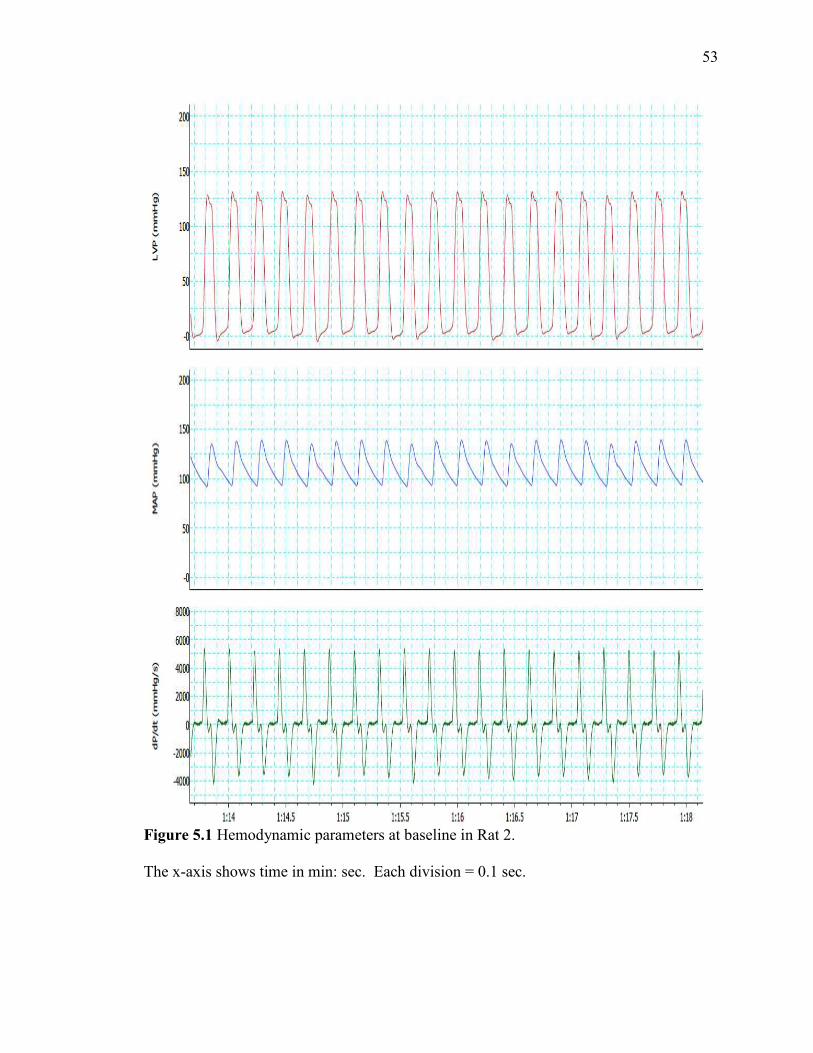
53
Figure 5.1 Hemodynamic parameters at baseline in Rat 2. The x-axis shows time in min: sec. Each division = 0.1 sec.

54
Figure 5.2 Hemodynamic parameters during the beginning of reference blood flow withdrawal under baseline conditions.
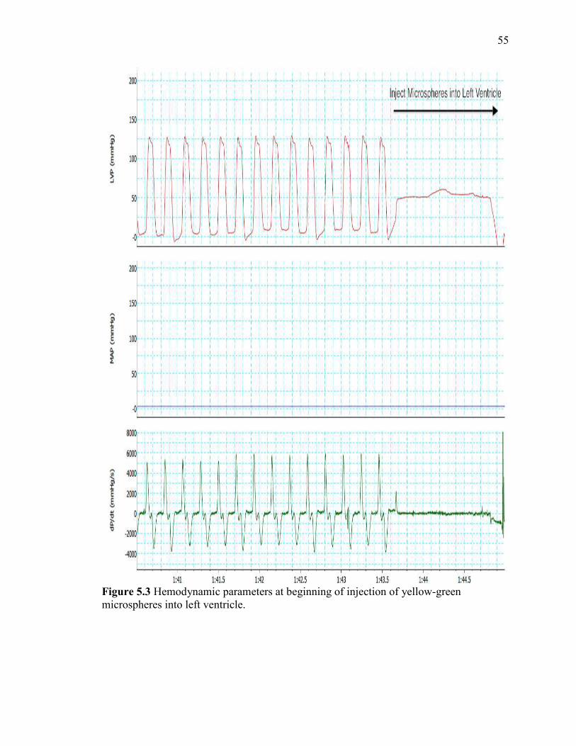
55
Figure 5.3 Hemodynamic parameters at beginning of injection of yellow-green microspheres into left ventricle.

56
Figure 5.4 Hemodynamic parameters after re-stabilization before infusion of adenosine

57
Figure 5.5 Hemodynamic parameters after attaining steady state under adenosine
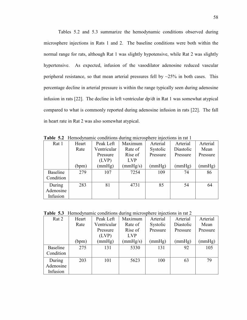
58
Tables 5.2 and 5.3 summarize the hemodynamic conditions observed during
microsphere injections in Rats 1 and 2. The baseline conditions were both within the
normal range for rats, although Rat 1 was slightly hypotensive, while Rat 2 was slightly
hypertensive. As expected, infusion of the vasodilator adenosine reduced vascular
peripheral resistance, so that mean arterial pressures fell by ~25% in both cases. This
percentage decline in arterial pressure is within the range typically seen during adenosine
infusion in rats [22]. The decline in left ventricular dp/dt in Rat 1 was somewhat atypical
compared to what is commonly reported during adenosine infusion in rats [22]. The fall
in heart rate in Rat 2 was also somewhat atypical.
Table 5.2 Hemodynamic conditions during microsphere injections in rat 1
Rat 1 Heart Rate
(bpm)
Peak Left Ventricular
Pressure (LVP)
(mmHg)
Maximum Rate of Rise of LVP
(mmHg/s)
Arterial Systolic Pressure
(mmHg)
Arterial Diastolic Pressure
(mmHg)
Arterial Mean
Pressure
(mmHg) Baseline
Condition 279 107 7254 109 74 86
During Adenosine Infusion
283 81 4731 85 54 64
Table 5.3 Hemodynamic conditions during microsphere injections in rat 2 Rat 2 Heart
Rate
(bpm)
Peak Left Ventricular
Pressure (LVP)
(mmHg)
Maximum Rate of Rise of LVP
(mmHg/s)
Arterial Systolic Pressure
(mmHg)
Arterial Diastolic Pressure
(mmHg)
Arterial Mean
Pressure
(mmHg) Baseline
Condition 275 131 5330 131 92 105
During Adenosine Infusion
203 101 5623 100 63 79

59
After the microsphere injection procedures, the rats were euthanized with an
overdose of anesthetic. The chest was opened and the heart was removed. The atria,
great vessels, and right ventricular free wall were all trimmed away, so that only the left
ventricle (including septum) remained. This heart tissue and the 2 blood samples were
then further processed by the procedure explained in Chapter 4 to recover the fluorescent
microspheres from the samples. Briefly, the samples were digested in 2.3 M ethanolic
KOH and 0.25 % Tween 80 for a period of 48 hours. At the end of digestion,
microspheres were recovered by the sedimentation method and the fluorescent dye was
extracted from them by using 3 ml of 2-ethoxy-ethyl-acetate.
5.2 Measurement of Microsphere Number in Tissue and Blood Samples
5.2.1 Measurement of fluorescence intensity
On the last day of the sedimentation procedure, the samples were read for
fluorescence intensity. Since microspheres of two different colors were used in the
procedure, samples were read at two different (excitation / emission) wavelengths. By
selecting filters in the spectrophotometer instrument, samples containing yellow-green
microspheres were read at (485 nm / 530 nm) (excitation / emission) wavelengths, and
samples containing red microspheres were read at (590 nm/ 645 nm) (excitation /
emission) wavelengths. After setting the filters, the samples were placed in a 96 well
plate reader and then scanned to measure fluorescence intensity (If). The intensities
measured are reported in Tables 5.4 and 5.5.

60
5.2.2 Calculation of number of fluorescent microspheres from calibration curves
The standard curves for fluorescent microspheres as obtained in Chapter 2 were
expressed by the following linear relationships:
For yellow-green microspheres: If = 0.9256 (Ns) – 4.9102
For red microspheres: If = 1.0954 (Ns) + 0.8414
where, If = fluorescence intensity obtained from spectrophotometer
Ns = number of fluorescent microspheres
Using these equations for the standard curves and knowing the values of
fluorescence intensity from the spectrophotometer, the number of fluorescent
microspheres can be determined.
To determine the number of yellow green microspheres in both blood and tissue samples:
Ns = (If + 4.9102) / 0.9256
To determine the number of red microspheres in both blood and tissue samples:
Ns = (If – 0.8414) / 1.0954
These inverse expressions of the standard curves were used to infer the number of
microspheres in each sample (Ns) from the measured value of fluorescence intensity (If).
The results for all samples from Rats 1 and 2 are shown in Tables 5.4 and 5.5.

61
Table 5.4 Number of fluorescent microspheres in blood and tissue samples in rat 1 Rat 1 Sample If Ns
Baseline : yellow-
green microspheres
Tissue 16782 18136
Baseline : yellow-
green microspheres
Blood 2007 2174
Adenosine : red
microspheres
Tissue 50438 46045
Adenosine : red
microspheres
Blood 2748 2508
Table 5.5 Number of fluorescent microspheres in blood and tissue samples in rat 2 Rat 2 Sample If Ns
Baseline : yellow-
green microspheres
Tissue 18943 20471
Baseline : yellow-
green microspheres
Blood 2128 2304
Adenosine : red
microspheres
Tissue 56700 51761
Adenosine : red
microspheres
Blood 2969 2710
5.3 Calculation of Coronary Blood Flow and Coronary Flow Reserve
Coronary blood flow delivers oxygen rich blood to heart muscle. The amount of blood
flow increases in proportion to the amount of heart muscle. For this reason, coronary
blood flow is expressed as flow per gram of tissue (ml/min/g). Microspheres serve as a
tracer of blood flow, so that the relative amounts of blood flow in two tissue samples are
proportional to the relative numbers of microspheres in each tissue. Thus,
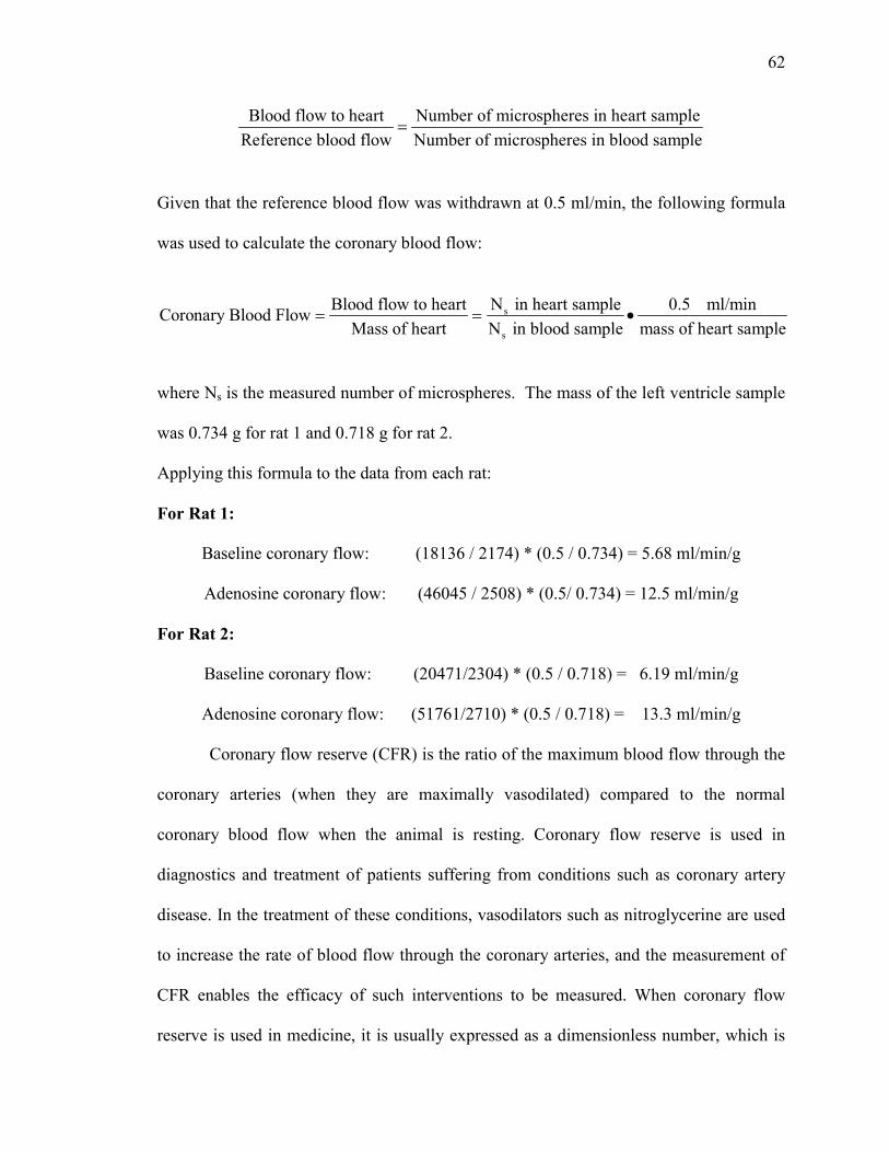
62
Blood flow to heart Number of microspheres in heart sampleReference blood flow Number of microspheres in blood sample
=
Given that the reference blood flow was withdrawn at 0.5 ml/min, the following formula
was used to calculate the coronary blood flow:
s
s
Blood flow to heart N in heart sample 0.5 ml/minCoronary Blood Flow
Mass of heart N in blood sample mass of heart sample= = •
where Ns is the measured number of microspheres. The mass of the left ventricle sample
was 0.734 g for rat 1 and 0.718 g for rat 2.
Applying this formula to the data from each rat:
For Rat 1:
Baseline coronary flow: (18136 / 2174) * (0.5 / 0.734) = 5.68 ml/min/g
Adenosine coronary flow: (46045 / 2508) * (0.5/ 0.734) = 12.5 ml/min/g
For Rat 2:
Baseline coronary flow: (20471/2304) * (0.5 / 0.718) = 6.19 ml/min/g
Adenosine coronary flow: (51761/2710) * (0.5 / 0.718) = 13.3 ml/min/g
Coronary flow reserve (CFR) is the ratio of the maximum blood flow through the
coronary arteries (when they are maximally vasodilated) compared to the normal
coronary blood flow when the animal is resting. Coronary flow reserve is used in
diagnostics and treatment of patients suffering from conditions such as coronary artery
disease. In the treatment of these conditions, vasodilators such as nitroglycerine are used
to increase the rate of blood flow through the coronary arteries, and the measurement of
CFR enables the efficacy of such interventions to be measured. When coronary flow
reserve is used in medicine, it is usually expressed as a dimensionless number, which is
63
formed by dividing the maximal coronary blood flow by resting blood flow. This allows
for an objective view, which can aid diagnosis and treatment.
In the microsphere studies, coronary flow reserve was calculated as:
Coronary flow reserve = (Coronary blood flow)adenosine / (Coronary blood flow)basal
For rat 1:
Coronary flow reserve = (Coronary blood flow)adenosine / (Coronary blood flow)basal
= 12.5 / 5.68
= 2.20
For rat 2:
Coronary flow reserve = (Coronary blood flow)adenosine / (Coronary blood flow)basal
= 13.3 / 6.19
= 2.15
5.4 Comparison with Coronary Flow Reserve Measured using Doppler Echocardiography
Coronary flow reserve was also measured using Doppler echocardiography in a set of 6
male Sprague-Dawley rats of the same age and range of body weights as the two rats
used in the microsphere study. These rats were also anesthetized using the same method
as in the microsphere study. Since the rats in both studies were of the same strain, age,
gender,body mass, and anesthetic state, it was reasonable to assume that they should have
similar coronary flow reserves.
However, there is one essential difference between the microsphere flow
measurement and the ultrasound measurement: Doppler echocardiography measures the
velocity of blood movement (in mm/s), not the bulk flow of blood volume (in ml/s).
However, if the cross-sectional area of the blood vessel being imaged does not change
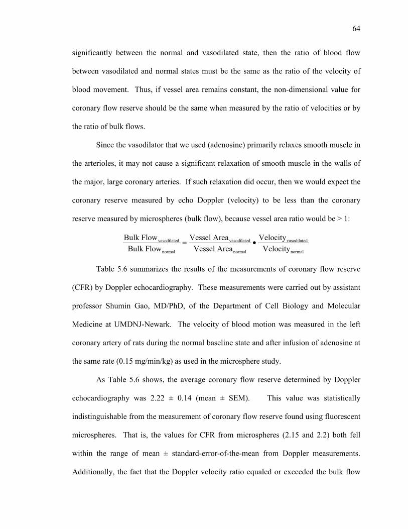
64
significantly between the normal and vasodilated state, then the ratio of blood flow
between vasodilated and normal states must be the same as the ratio of the velocity of
blood movement. Thus, if vessel area remains constant, the non-dimensional value for
coronary flow reserve should be the same when measured by the ratio of velocities or by
the ratio of bulk flows.
Since the vasodilator that we used (adenosine) primarily relaxes smooth muscle in
the arterioles, it may not cause a significant relaxation of smooth muscle in the walls of
the major, large coronary arteries. If such relaxation did occur, then we would expect the
coronary reserve measured by echo Doppler (velocity) to be less than the coronary
reserve measured by microspheres (bulk flow), because vessel area ratio would be > 1:
vasodilated vasodilated vasodilated
normal normal normal
Bulk Flow Vessel Area VelocityBulk Flow Vessel Area Velocity
= •
Table 5.6 summarizes the results of the measurements of coronary flow reserve
(CFR) by Doppler echocardiography. These measurements were carried out by assistant
professor Shumin Gao, MD/PhD, of the Department of Cell Biology and Molecular
Medicine at UMDNJ-Newark. The velocity of blood motion was measured in the left
coronary artery of rats during the normal baseline state and after infusion of adenosine at
the same rate (0.15 mg/min/kg) as used in the microsphere study.
As Table 5.6 shows, the average coronary flow reserve determined by Doppler
echocardiography was 2.22 ± 0.14 (mean ± SEM). This value was statistically
indistinguishable from the measurement of coronary flow reserve found using fluorescent
microspheres. That is, the values for CFR from microspheres (2.15 and 2.2) both fell
within the range of mean ± standard-error-of-the-mean from Doppler measurements.
Additionally, the fact that the Doppler velocity ratio equaled or exceeded the bulk flow
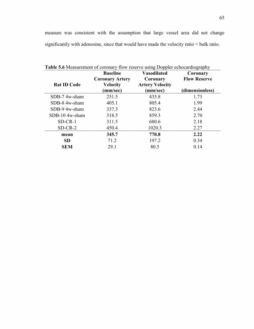
65
measure was consistent with the assumption that large vessel area did not change
significantly with adenosine, since that would have made the velocity ratio < bulk ratio.
Table 5.6 Measurement of coronary flow reserve using Doppler echocardiography
Rat ID Code
Baseline Coronary Artery
Velocity (mm/sec)
Vasodilated Coronary
Artery Velocity (mm/sec)
Coronary Flow Reserve
(dimensionless) SDB-7 4w-sham 251.5 435.8 1.73 SDB-8 4w-sham 405.1 805.4 1.99 SDB-9 4w-sham 337.3 823.6 2.44
SDB-10 4w-sham 318.5 859.3 2.70 SD-CR-1 311.5 680.6 2.18 SD-CR-2 450.4 1020.3 2.27
mean 345.7 770.8 2.22 SD 71.2 197.2 0.34
SEM 29.1 80.5 0.14
66
CHAPTER 6
DISCUSSION AND FUTURE WORK
The present study shows that fluorescent microspheres can be used to reliably determine
coronary blood flow in rats under baseline conditions and after infusion with adenosine.
There were no significant differences observed in coronary flow reserve measured with
either Doppler echocardiography or fluorescent microspheres. In addition, the absolute
value of baseline coronary flow obtained in this study agreed well with the value
published in a recent study on rats [22].
Fluorescent microspheres were used in this study. This technique has thus been
demonstrated to be a reliable alternative to radioactive or colored microspheres for
measuring organ blood flow in rats under normal conditions and under infusion with
adenosine. In the present study, supernatants and pure microsphere samples were
analyzed from each step of the tissue recovery protocol, which suggested that there was
100% recovery of microspheres regardless of mass and blood flow capacity. The
sedimentation method for the recovery of fluorescent microspheres was achieved by use
of ethanolic solutions, which increased the specific gravity difference between
microspheres and medium, aided by higher centrifugation speeds that avoided the loss of
fluorescent microspheres.
The resolution of the fluorescence method is dependent on the amount of label per
microsphere, the quantum efficiency of the fluorescent dye, and the sensitivity of the
spectrophotometer. The latter is determined by light source intensity, transmittance of
filters or monochromators used to select excitation and emission wavelengths, efficiency
of photomultiplier tube, and the type of plate reader used. By using optimal excitation

67
and emission wavelengths, there was very good correlation between fluorescence
intensity and number of microspheres across a wide range of concentrations.
Although we had crimson fluorescent microspheres as an option along with the
red and yellow-green microspheres that we used, we did not use crimson because of its
low quantum efficiency and significant spillover into adjacent colors at higher
concentrations.
When two different colors of fluorescent microspheres were injected into the
body of a rat under baseline conditions and under infusion of adenosine, there was a good
relation between estimated blood flow across a wide range of tissue blood flow.
Fluorescent microspheres produced no significant alteration in blood pressure during or
after injection in rats. Use of red and yellow-green microspheres resulted in no spillover
in the course of this study.
A dilution procedure was performed using known microsphere samples to
obtain the calibration curve of fluorescence intensity versus microsphere number. Several
trials of the dilution procedure were performed on each of the two microsphere colors. A
linear regression equation was obtained for each graph plotted. These regressions were
then averaged to obtain an standard curve for each fluorescent microsphere color that we
used. Averaging increased the accuracy of the calibration thus resulting in a more reliable
final value of coronary blood flow.
Because of the small blood volume in rats, we limited our investigation to two
successive measurements by taking two reference blood samples each of 1 ml. We
calculated that – compared to the weight of the animal – this volume of reference blood
withdrawn was less than 10% of the total blood volume in each rat, which should not

68
have affected the hemodynamics of the animal. In addition, after each reference blood
withdrawal, saline was inflused into the rat which also helped to restore blood volume.
Our study demonstrates that the fluorescent microsphere method is able to
accurately reflect the increase in flow that occurs in rats after infusion of a coronary
vasodilator, adenosine. Adenosine infusion produced nearly identical increases in
myocardial blood flow (measured by fluorescnt microspheres) and in coronary blood
velocity (measured by Doppler echocardiography). The mean coronary blood flow
reserve obtained by the fluorescent microsphere method was 2.18, which was within the
standard estimate of the value for coronary flow velocity reserve obtained by the range-
gated Doppler echocardiography method.
As reported in a recently published article [22], the value of mean myocardial
blood flow in Sprague Dawley rats at baseline and after infusion with adenosine, were 5.9
+/- 2.3 (ml/min/g) and 13.1+/-2.1(ml/min/g), respectively. In our study, using the same
species of rat and the same coronary vasodilator, the values obtained at baseline and after
infusion with adenosine were 5.94 and 12.9 (ml/min/g), respectively. Thus, the values
we observed in both conditions (baseline + vasodilated) fall within the 95% confidence
interval of this recently reported data. This suggests that the procedures developed in this
thesis for microsphere recovery (by the sedimentation method) and fluorescence
measurement and calibration offer a reliable method for determining coronary blood flow
in rats.
Colored microspheres are currently being used to determine coronary blood
flow in rats in the laboratories of the Cellular Biology and Molecular Medicine
Department at UMDNJ, Newark. We were thus able to collaborate with current expertise
69
in microsphere injection procedures, and this collaboration undoubtedly improved the
reliability of our results compared to what we would have been able to achieve
independently. However, the samples of tissue and blood containing colored
microspheres are currently sent out to a commercial processor to determine the number of
microspheres and hence coronary blood flow. The techniques applied in this thesis are
thus new to this laboratory and offer a reasonable alternative to commercial processing to
measure coronary blood flow.
One drawback of our study is that only two animals were used for the procedure.
This was due to the busy schedule of the collaborators at UMDNJ and the limited time
window in which this thesis had to be completed. However, the quality of agreement
among the two studies that were performed – and their agreement with recent data
reported in the literature – suggests that a larger study might have even more strongly
supported the repeatability of the results.
In the future, it would be important to see whether the fluorescent microsphere
method could also be applied to measure coronary blood flow in mice. We attempted
two experiments on mice, but we experienced failure during the cardiac cannulation
procedure. It appeared that the catheter used was too large in diameter and thus too stiff
to be able to be guided into the left ventricle of mice. Use of a smaller diameter catheter
might offer easier access to the left ventricle, however one would also have to evaluate
whether microspheres could be injected at an adequate rate through such a smaller
diameter. Also, due to the very small blood volume of a mouse, it will be more difficult
to obtain two reference blood samples without affecting the hemodynamics of the mouse.
Finally, to achieve accurate measurements [38] sufficient numbers of microspheres will
70
have to be injected so that at least 400-500 spheres will be trapped in the left ventricular
tissue (which typically has a mass of only 80-100 micrograms) and in each reference
blood sample.
Note that during the dilution procedure to obtain the calibration curves we used
whole microspheres from the stock solution (with the fluorescent dye remaining within
the microspheres). On the other hand, during the actual procedure after microspheres
were recovered from the body of animal, the microspheres were dissolved chemically to
release the dye into solution. We believe this is an adequate calibration procedure
because only the ratio of fluorescent intensities matters in the determination of blood
flow. Because our calibrations showed that fluorescent intensity was linearly related to
microsphere number throughout the range of interest, the ratio of intensities will be the
same as the ratio of numbers. Each microsphere dye might produce more intensity when
free in solution because of limits to excitation and absorption of emitted light imposed
when the dye remains inside a microsphere. However, we assumed that this effect
would apply equally to both the tissue and reference blood samples. Thus, the ratio of
fluorescent intensity would not be affected by whether the dye was in solution or
remained within the microspheres.
In conclusion, the fluorescent microsphere technique (a) is a reliable method for
measuring coronary blood flows in rats; (b) works well as a substitute for radioactive or
colored microspheres, with advantages in safety and cost; and (c) provides repeatable
measurements allowing at least two flow measurements in the same animal.
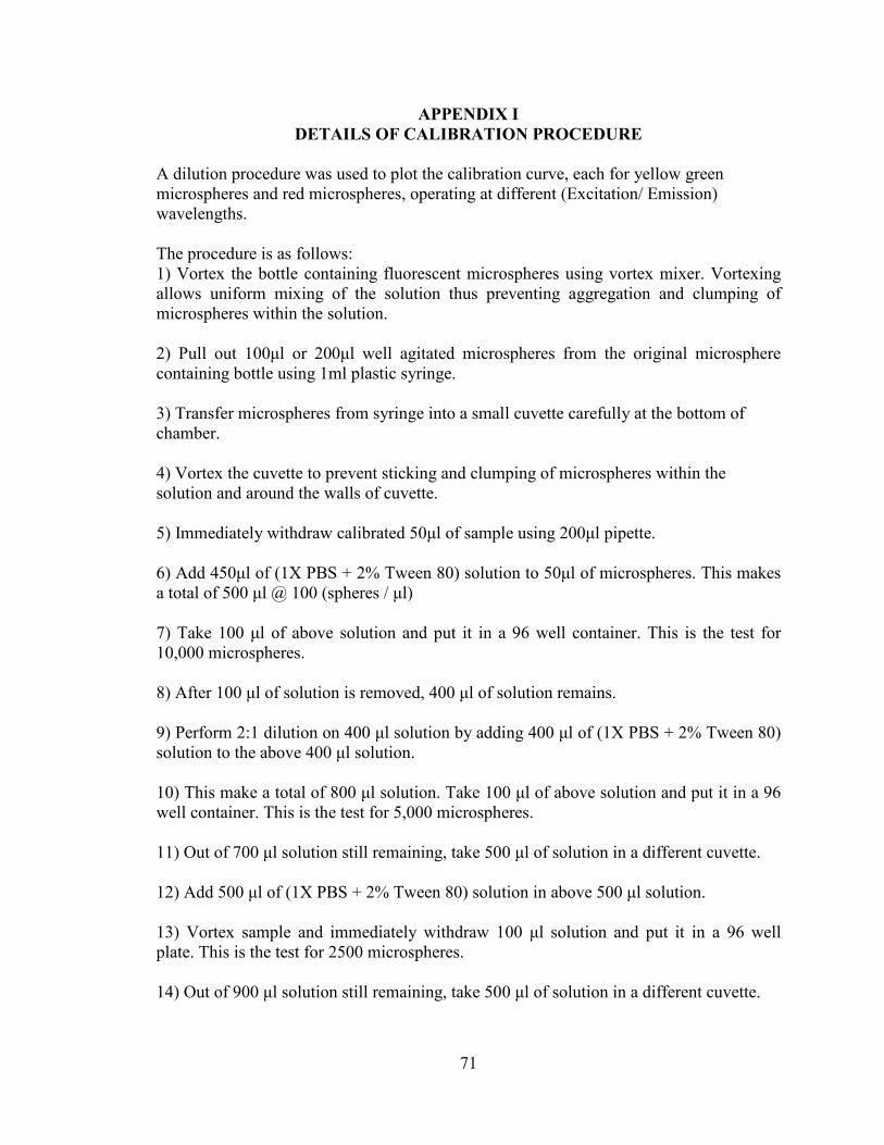
71
APPENDIX I DETAILS OF CALIBRATION PROCEDURE
A dilution procedure was used to plot the calibration curve, each for yellow green microspheres and red microspheres, operating at different (Excitation/ Emission) wavelengths. The procedure is as follows: 1) Vortex the bottle containing fluorescent microspheres using vortex mixer. Vortexing allows uniform mixing of the solution thus preventing aggregation and clumping of microspheres within the solution. 2) Pull out 100µl or 200µl well agitated microspheres from the original microsphere containing bottle using 1ml plastic syringe. 3) Transfer microspheres from syringe into a small cuvette carefully at the bottom of chamber. 4) Vortex the cuvette to prevent sticking and clumping of microspheres within the solution and around the walls of cuvette. 5) Immediately withdraw calibrated 50µl of sample using 200µl pipette. 6) Add 450µl of (1X PBS + 2% Tween 80) solution to 50µl of microspheres. This makes a total of 500 µl @ 100 (spheres / µl) 7) Take 100 µl of above solution and put it in a 96 well container. This is the test for 10,000 microspheres. 8) After 100 µl of solution is removed, 400 µl of solution remains. 9) Perform 2:1 dilution on 400 µl solution by adding 400 µl of (1X PBS + 2% Tween 80) solution to the above 400 µl solution. 10) This make a total of 800 µl solution. Take 100 µl of above solution and put it in a 96 well container. This is the test for 5,000 microspheres. 11) Out of 700 µl solution still remaining, take 500 µl of solution in a different cuvette. 12) Add 500 µl of (1X PBS + 2% Tween 80) solution in above 500 µl solution. 13) Vortex sample and immediately withdraw 100 µl solution and put it in a 96 well plate. This is the test for 2500 microspheres. 14) Out of 900 µl solution still remaining, take 500 µl of solution in a different cuvette.

72
15) Add 500 µl of (1X PBS + 2% Tween 80) solution in above 500 µl solution. 16) Vortex sample and immediately withdraw 100 µl solution and put it in a 96 well plate. This is the test for 1250 microspheres. 17) Out of 900 µl solution still remaining, withdraw 500 µl of solution in a different cuvette. 18) Add 500 µl of (1X PBS + 2% Tween 80) solution in above 500 µl solution. 19) Vortex sample and immediately withdraw 100 µl solution and put it in a 96 well plate. This is the test for 625 microspheres. 20) Out of 900 µl solution still remaining, withdraw 500 µl of solution in a different cuvette 21) Add 500 µl of (1X PBS + 2% Tween 80) solution in above 500 µl solution. 22) Vortex sample and immediately withdraw 100 µl solution and put it in a 96 well plate. This is the test for 312 microspheres. 23) The 96 well plate is then placed in a plate reader to determine the fluorescence intensity. Depending on the color of fluorescent microspheres, the (Excitation / Emission) wavelengths are set in the instrument and then a scan is carried out to determine the fluorescence intensity.

73
APPENDIX II
CALIBRATION CURVES FOR FIVE TESTS PERFORMED ON EACH
MICROSPHERE COLOR
A dilution procedure as described in Chapter 2 was performed five times with each
microsphere color to get an average calibration curve. With each trial, the readings were
recorded on spectrophotometer and graphs were plotted on Microsoft Excel. The
intercept equations for each trials were then averaged together to get a standard
calibration curve. Yellow- green microspheres were used for getting a calibration curve
which can be used for baseline calculations. Red microspheres were used for getting a
calibration curve which can be used for vasodilation calculations.
Trials done with yellow- green microspheres:
Sample 1:
Table 2.2 Representation of fluorescent intensities at various dilutions
Microsphere number Fluorescence Intensity
10000 11363
5000 5964
2500 2808
1250 1407
625 717
312 318

74
Figure 2.4 Excel plots showing the 1st baseline calibration curve
Sample 2:
Table 2.3 Representation of fluorescent intensities at various dilutions
Microsphere number Fluorescence Intensity
10000 9214
5000 4400
2500 2150
1250 1000
625 550
312 300
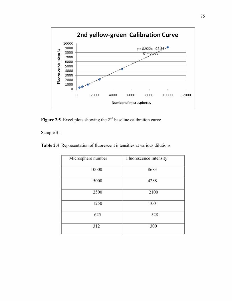
75
Figure 2.5 Excel plots showing the 2nd baseline calibration curve
Sample 3 :
Table 2.4 Representation of fluorescent intensities at various dilutions
Microsphere number Fluorescence Intensity
10000 8683
5000 4288
2500 2100
1250 1001
625 528
312 300

76
Figure 2.6 Excel plots showing the 3rd baseline calibration curve
Sample 4:
Table 2.5 Representation of various fluorescent intensities at various dilutions
Microsphere number Fluorescence Intensity
10000 9110
5000 4792
2500 2000
1250 1068
625 629
312 308

77
Figure 2.7 Excel plots showing the 4th baseline calibration curve
Sample 5:
Table 2.6 Representation of various fluorescent intensities at various dilutions
Microsphere number Fluorescence Intensity
10000 7752
5000 4245
2500 2039
1250 1200
625 501
312 284
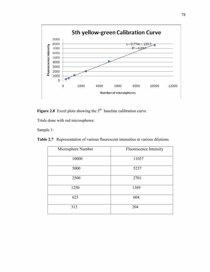
78
Figure 2.8 Excel plots showing the 5th baseline calibration curve
Trials done with red microspheres:
Sample 1:
Table 2.7 Representation of various fluorescent intensities at various dilutions.
Microsphere Number Fluorescence Intensity
10000 11057
5000 5237
2500 2701
1250 1389
625 604
312 204

79
Figure 2.9 Excel plots showing the 1st vasodilation calibration curve
Sample 2:
Table 2.8 Representation of various fluorescent intensities at various dilutions. Microsphere Number Fluorescence Intensity
10000 8991
5000 4477
2500 1819
1250 867
625 507
312 394

80
Figure 2.10 Excel plots showing the 2nd vasodilation calibration curve
Sample 3: Table 2.9 Representation of various fluorescent intensities at various dilutions
Microsphere Number Fluorescence Intensity
10000 11573
5000 6171
2500 3000
1250 1682
625 800
312 500

81
Figure 2.11 Excel plots showing the 3rd vasodilation calibration curve Sample 4: Table 2.10 Representation of various fluorescent intensities at various dilutions
Microsphere Number Fluorescence Intensity
10000 11100
5000 6263
2500 3623
1250 1798
625 1000
312 450

82
Figure 2.12 Excel plots showing the 4th vasodilation calibration curve
Sample 5: Table 2.11 Representation of various fluorescent intensities at various dilutions
Microsphere Number Fluorescence Intensity
10000 12306
5000 6055
2500 2930
1250 1611
625 827
312 430

83
Figure 2.13 Excel plots showing the 5th vasodilation calibration curve
84
REFERENCES [1] Austin GE, Tuvlin MB, Martino-Salzman D, Hunter RL, Justicz, AG, Thompson NK, Brooks AC (1993), Determination of regional myocardial blood flow using fluorescent microspheres; American Journal of Cardiovascular Pathology;4:352-7. [2] Bernard SL, Ewen JR, Barlow CH, Mckinney S, Glenny RW (2000), High spatial resolution measurements of organ blood flow in small laboratory animals, American Journal of Physiology: Heart and Circulatory Physiology,279:H2043-52. [3] Bio-Tek Instruments (1996): Bio-Tek FL500 Fluorescence Plate Reader User Guide (revision B) [4] Buchwalder LF, Lin M., McDonald TJ. and Nathanielsz PW. (1998), Fetal sheep adrenal blood flow responses to hypoxemia after splanchnicotomy using fluorescent microspheres, Journal of Applied Physiology 84, 82-89 [5]http://www.cbsnews.com/stories/2005/03/18/earlyshow/saturday/main681597.shtml, Article in the news: How to take care of your heart. [6] Chien GL, Anselone CG, Davis RF. and Van Winkle DM. (1995), Fluorescent vs. radioactive microsphere measurement of regional myocardial blood flow, Cardiovascular Research 30, 405-412 [7]http://www.cvphysiology.com/Blood%20Flow/BF001.htm,Cardiovascular Physiology Concepts, Richard. E. Klabunde, PhD, 2005 [8] Degens H, Craven, AJ, Jarvis JC and Salmons S. (1996), The use of colored dye-extraction microspheres to measure blood flow in rabbit skeletal muscle: a validation study with special emphasis on repeated measurements. Experimental Physiology 81, 239-249 [9] De Visscher G, Haseldonckx M, Flameng W (2006), Fluorescent microsphere technique to measure cerebral blood flow in the rat, Nature Protocol.1:2162-70. [10] http://www.echoincontext.com/doppler01/doppler01_09.asp, Duke Medical Center (2000), Pulsed and continuous wave Doppler, Pages 1-2 [11] http://ehs.uc.edu/lams/index.html, William P. Porter (2000), American College of Laboratory Animal Medicine, “Laboratory Medical Medicine and Science Series II, Rats and Mice: Introduction and Use in Research Part I, Pages 6-9 [12] http://ehs.uc.edu/lams/index.html, David M. Moore (2000), American College of Laboratory Animal Medicine, “Laboratory Medical Medicine and Science Series II, Rats and Mice: Introduction and Use in Research Part II, Pages 4, 9

85
[13] Glenny RW, Bernard S, Brinkley M. (1993), Validation of fluorescent-labeled microspheres for measurement of regional organ perfusion; Journal of Applied Physiology, 74 (5), 2585-97 [14] Gronos J, Wikstrom J, Hagg U, Wandt B, Gan LM (2006), Proximal to middle left coronary artery flow velocity ratio, as assessed using color doppler echocardiography, predicts coronary artery atherosclerosis in mice, Arteriosclerosis, Thrombosis, and Vascular Biology.26:1126-1131. [15] Hagg U, Gronros J, Wikstrom J, Ingiborg H. Jonsdottir, Bergstrom G and Gan LM, (2005), Voluntary physical exercise and coronary flow velocity reserve: a transthoracic colour Doppler echocardiography study in spontaneously hypertensive rat, Clinical Science;109, 325–334 [16] Hale SL, Kevin BS, Alker J and Kloner RA. (1988), Evaluation of nonradioactive, colored microspheres for measurement of regional myocardial blood flow in dogs. Circulation 78, 428-434 [17]http://heartdisease.about.com/cs/starthere/a/corartanat.htm, Anatomy of Normal Coronary Arteries, Richard N. Fogoros, M.D., December 2003 [18]http://health.msn.com/health-topics/cholesterol/why-healthy-people-suffer-heart-attacks, Article: Why healthy people suffer heart attacks, Dr. Arthur Agatston [19] Hecht R, Habler O, Kleen M, Welte M, Staub F, Frey L. and Mesmer K. (1995), New perspectives through automation of the fluorescent microsphere technique for determination of regional blood flow, FASEB Journal 9, A908 (Abstract) [20] Hozumi T, MD, Yoshida K, Akasaka T, Asami Y, (1998), Noninvasive assessment of coronary flow velocity and coronary flow velocity reserve in the left anterior descending coronary artery by doppler echocardiography, Journal of the American College of Cardiology,32:1251–9 [21]http://www.invitrogen.com/site/us/en/home/References/Molecular-Probes-The-Handbook/tables/FluoSpheres-microspheres-for-blood-flow-determination.html [22] Jacquier A, Kober F, Bun S, Giorgi R, Cozzone P.J and Bernard M, (2011), Quantification of myocardial blood flow and flow reserve in rats using arterial spin labeling MRI: comparison with a fluorescent microsphere technique. NMR in Biomedicine, doi: 10 1002/ nbm.1645 [23] Kowallik P, Schulz R, Guth BD, Schade A , Paffhausen W, Gross R. and Heusch G. (1991), Measurement of regional myocardial blood flow with multiple colored microspheres. Circulation 83, 974-982
86
[24] Lakowicz J.R, Principles of Fluorescence Spectroscopy (2nd edition) (2004), New York: Springer, Pages 1 -12 [25] McKirnan MD., Williams RL, Lohman JL, Eising GP, Hammond HK. & Ross J. (1994), Blood flow measurements during myocardial ischemia and dysfunction using fluorescent labeled Microspheres, FASEB Journal 8, A857 (Abstract) [26] http://microspheres.net/Nuflow-Protocol.pdf, NuFLOW fluorescent microsphere extraction protocol for regional blood flow measurement, Interactive Medical Technology, Revised March 2001, Pages 1-2 [27] Mori H, Haruyama S, Shinozaki Y, Okino H, Iida A, Takanashi R, Sakuma I, Husseini, WK, Payne BD. & Hoffman JIE. (1992), New nonradioactive microspheres and more sensitive X ray fluorescence to measure regional blood flow, American Journal of Physiology 263, H 1946-1957 [28] Morita Y, Payne BD, Aldea GS, McWaters C, Husseini W, Mori H, Hoffman JIE. and Kaufman L. (1990), Local blood flow measured by fluorescence excitation of nonradioactive Microspheres, American Journal of Physiology 258, H 1573-1584 [29] Mulder TLM, Van Golde JC, Prinzen FW. and Blanco CE. (1997), Cardiac output distribution in the chick embryo from stage 36 to 45. Cardiovascular Research 34, 525-528. [30] National Academies Press (1988), “Use of Laboratory Animals in Biomedical and Behavioral Research”, Washington DC, Pages 31-32 [31] Prinzen FW, Bassingthwaigthe JB. (2000), Blood flow distributions by microsphere deposition methods, Cardiovascular Research 45: 13-21. [32] Prinzen FW. and Glenny RW. (1994), Developments in non-radioactive microsphere techniques for blood flow measurements, Cardiovascular Research 28, 1467-1475. [33] http://probes.invitrogen.com/media/spectra/8811h2o.jpg [34] Richer C, Domergue V, Gervais M, Bruneval P, Giudicelli JF (2000), Fluospheres for cardiovascular phenotyping genetically modified mice, Journal of Cardiovascular Pharmacology,36;396-404 [35] Rudolph, AM and Heymann, MA (1967), The circulation of fetus in utero: Methods of studying distribution of blood flow, cardiac output and organ blood flow, Circulation Research; 21; 163-184 [36] Serrat MA (2009), Measuring bone blood supply in mice using fluorescent microspheres, Nature Protocols.;4:1749-58.

87
[37] http://www.uptodate.com/contents/principles-of-doppler-echocardiography, Warren J Manning, Nelson B Schiller (2010), “Principles of Doppler Echocardiography”, Pages 1-10 [38] Van Oosterhout, M. F. M., Willigers, H. M. M., Reneman, R. S. & Prinzen, F. W. (1995). Fluorescent microspheres to measure organ perfusion: validation of a simplified sample processing technique, American Journal of Physiology 269, H725-733 [39] http://fmrcc.pulmcc.washington.edu/documents/fmrcman99.pdf, Manual for using fluorescent microspheres to measure regional organ perfusion, Fluorescent microsphere resource center, University of Washington, Revised October 1, 1999.


