

CORRECTION OF FINITE SIZE ERRORS IN MANY-BODY
ELECTRONIC STRUCTURE CALCULATIONS
Hendra Kwee
Palembang, South Sumatra, Indonesia
Master of Science, College of William and Mary, 2002
Bachelor of Science, Institut Teknologi Bandung, 2001
A Dissertation presented to the Graduate Faculty
of the College of William and Mary in Candidacy for the Degree of
Doctor of Philosophy
Department of Physics
The College of William and Mary
January 2008

APPROVAL PAGE
This Dissertation is submitted in partial fulfillment of
the requirements for the degree of
Doctor of Philosophy
Hendra Kwee
Approved by the Committee, October 2007
Committee Chair
Professor Henry Krakauer, Physics
The College of William and Mary
Assistant Professor Joshua Erlich, PhysicsThe College of William and Mary
Professor Kenneth Petzinger, PhysicsThe College of William and Mary
Associate Professor Shiwei Zhang, PhysicsThe College of William and Mary
Professor Robert Vold, Applied ScienceThe College of William and Mary

ABSTRACT PAGE
Electronic structure calculations using simulation cells for extended systems
typically incorporate periodic boundary conditions as an attempt to mimic the real
system with a practically infinite number of particles. Periodic boundary conditions
introduce unphysical constraints that give rise to finite-size errors. In mean-field
type calculations, the infinite size limit is achieved by simple quadrature in the
Brillouin zone using a finite number of k-points. Many-body electronic structure
calculations with explicit two-particle interactions cannot avail themselves of this
simplification. Direct extrapolation is computationally costly while size correction
with less accurate methods is frequently not sufficiently accurate. The Hartree-Fock
method neglects the correlation energy, while the conventional density functional
theory (DFT) uses the infinite-size limit of the exchange correlation function. Here
we present a new finite-size exchange correlation function designed to be used in DFT
calculations to give more accurate estimates of the finite-size errors. Applications
of the method are presented, including the P2 molecule, fcc silicon, bcc sodium
and BiScO3 perovskite. The method is shown to deliver rapidly convergent size-
corrections.

Dedicated to my mother Heryawaty and the memory of my father Johnny Kwee.
iv

Table of Contents
Acknolwedgements . . . . . . . . . . . . . . . . . . . . . . . . . . . . . vii
List of Tables . . . . . . . . . . . . . . . . . . . . . . . . . . . . . . . . viii
List of Figures . . . . . . . . . . . . . . . . . . . . . . . . . . . . . . . . xi
CHAPTER
1 Introduction . . . . . . . . . . . . . . . . . . . . . . . . . . . . . 2
2 Electronic Structure Methods . . . . . . . . . . . . . . . . . . . 6
2.1 Introduction . . . . . . . . . . . . . . . . . . . . . . . . . . . . . . 6
2.2 Mean-field Type Methods . . . . . . . . . . . . . . . . . . . . . . 8
2.2.1 Hartree-Fock Method . . . . . . . . . . . . . . . . . . . . . 8
2.2.2 Density Functional Theory . . . . . . . . . . . . . . . . . . 10
2.3 Many-body methods . . . . . . . . . . . . . . . . . . . . . . . . . 12
2.3.1 Configuration Interaction . . . . . . . . . . . . . . . . . . . 12
2.3.2 Quantum Monte Carlo . . . . . . . . . . . . . . . . . . . . 14
3 Auxiliary Field Quantum Monte Carlo . . . . . . . . . . . . . 16
3.1 Conventions . . . . . . . . . . . . . . . . . . . . . . . . . . . . . . 17
3.2 Planewave Basis . . . . . . . . . . . . . . . . . . . . . . . . . . . . 20
3.3 Hamiltonian . . . . . . . . . . . . . . . . . . . . . . . . . . . . . . 21
3.4 Ground-State Projection . . . . . . . . . . . . . . . . . . . . . . . 25
v

4 Jellium . . . . . . . . . . . . . . . . . . . . . . . . . . . . . . . . 28
4.1 Hartree-Fock Solution to the Infinite-Size-Limit of Jellium System 30
4.2 Several Simple AFQMC Test Calculations . . . . . . . . . . . . . 32
4.3 Cutoff Energy Dependence of Jellium Correlation Energy . . . . . 34
5 Finite Size Effects . . . . . . . . . . . . . . . . . . . . . . . . . . 38
5.1 Origin of Finite Size Errors . . . . . . . . . . . . . . . . . . . . . . 39
5.2 Existing Correction Methods . . . . . . . . . . . . . . . . . . . . . 42
5.3 Finite Size Jellium Energy . . . . . . . . . . . . . . . . . . . . . . 45
5.3.1 Overview of Extrapolation Scheme . . . . . . . . . . . . . 45
5.3.2 Hartree-Fock Energy of Jellium . . . . . . . . . . . . . . . 47
5.4 Fitting the FS Exchange Correlation functional . . . . . . . . . . 49
6 Applications of Finite Size Correction . . . . . . . . . . . . . . 59
6.1 Correction Scheme . . . . . . . . . . . . . . . . . . . . . . . . . . 59
6.2 P2 Molecule . . . . . . . . . . . . . . . . . . . . . . . . . . . . . . 65
6.3 Fcc Silicon . . . . . . . . . . . . . . . . . . . . . . . . . . . . . . . 67
6.4 Bcc Sodium . . . . . . . . . . . . . . . . . . . . . . . . . . . . . . 76
6.5 Perovskite BiScO3 . . . . . . . . . . . . . . . . . . . . . . . . . . . 81
7 Conclusion and Outlook . . . . . . . . . . . . . . . . . . . . . . 87
APPENDIX APseudopotential . . . . . . . . . . . . . . . . . . . . . . . . . . . . . 89
APPENDIX BDependence of the Jellium Correlation Energy on the Cutoff En-ergy Ecut . . . . . . . . . . . . . . . . . . . . . . . . . . . . . . . . . 94
APPENDIX CTechnical Details of the BiScO3 Calculation . . . . . . . . . . . . 102
Bibliography . . . . . . . . . . . . . . . . . . . . . . . . . . . . . . . . . 104
Vita . . . . . . . . . . . . . . . . . . . . . . . . . . . . . . . . . . . . . . 110
vi

ACKNOWLEDGMENTS
First of all, I would like to express my deepest gratitude to my advisors, Profes-sor Henry Krakauer and Professor Shiwei Zhang, for their support, encouragementand continual guidance during the entire course of this research. Their deep com-mitment to this project and also to my professional development as a physicist isgreatly appreciated. I also would like to acknowledge the members of our researchgroup, thanking especially Dr. Wirawan Purwanto and Dr. Eric Walter for theirgreat help.
I would like to thank the Ph.D. defense committee members for their carefulexamination and correction of my thesis. I would also like to thank the physicsdepartment administrative staff, Carol Hankins, Paula Perry, and Sylvia Stout, fortheir excellent work. Without them, nothing would be accomplished.
I also want to thank Herry Kwee for being a good brother and role modelfor me, and Agus Ananda for being a great friend. They both provided wise adviseand encouragement, which is much appreciated. I also want to thank my roommatesJong Anly Tan and Zainul Abidin for all their support in the past few years. Specialthanks for the friends that I have met in this country, Steve Richardson and ZhangBo. Thank you for the great friendship we have; I will miss you. I also want tothank two families that have been very kind to me. The first is Pastor Tom and hiswife Cheryl Darnell; thank you for your sincere care, prayer and hospitality for me.The second family is Stan and Debbie Betz; thank you for your support and prayerfor me.
Finally I want to thank Dr. Yohanes Surya for giving me a recommendationletter when I applied to graduate school here in the college of William and Mary.Also special thanks to my overseas friends Samuel Bangun Wibowo and JemmyNatanael Patras. Thank you for the many hours of conversations and encouragementover the last few years of my study here.
vii
LIST OF TABLES
4.1 Correlation energy per electron of jellium with number of electrons
N = 14. The average distance of the electrons rs is 4.0. The results
are compared with other AFQMC calculations (see Ref. [43] and also
see discussion on Ref. [44]). All quantities are in Rydberg atomic unit. 33
4.2 Energy per electron of jellium with number of electrons N = 54. L
is the size of the cubic box. The error of the calculation is given in
the last digit. All quantities are in the Rydberg atomic unit . . . . . 33
5.1 The parameters in the B1(rs) and B2(rs). All parameters are given
in Rydberg atomic unit . . . . . . . . . . . . . . . . . . . . . . . . . . 47
5.2 Summary of the FS exchange and correlation functions . . . . . . . . 56
5.3 Numerical values of parameters used in Table. 5.2. All parameters
are given in Rydberg atomic unit. . . . . . . . . . . . . . . . . . . . . 57
6.1 The pseudopotentials that are used to test the dependence of the two-
body FS correction on pseudopotentials. The first three pseudopo-
tentials were obtained from the OPIUM code [30], and the fourth one
is the Goedecker-Teter-Hutter pseudopotential [63]. rc is the cut-off
radius of the pseudopotential in Bohr. . . . . . . . . . . . . . . . . . 68
6.2 Several physical properties calculated with the four pseudopotentials
in Table. 6.1. The results are compared with our own all electron
LAPW results and with the pseudopotential and LAPW calculations
from Ref. [64]. . . . . . . . . . . . . . . . . . . . . . . . . . . . . . . . 69
6.3 The two-body correction for 4 pseudopotentials (in eV). Na is the
number of atoms. The parameter L indicates the effective volume
of the cell L = Ω1/3 (in Bohr). Results are shown for fcc and cubic
supercells. . . . . . . . . . . . . . . . . . . . . . . . . . . . . . . . . . 70
viii

6.4 The equilibrium lattice constant, bulk modulus and cohesive energy
of silicon bulk. Na is the number of atoms used in calculations. TBC
2 and TBC 4 are twist-averaged boundary condition [52] based on
2×2×2 and 4×4×4 Mankhorst-Pack [50] k-point grids, respectively.
∆E = ∆E1−b + ∆E2−b. The cohesive energies contain a correction
for the zero-point energy of the solid of EZPE=0.06 eV per atom. . . . 75
6.5 The equilibrium lattice constant and bulk modulus of solid sodium
calculated with DFT. Calculations with and without semicore states
are shown as well as all-electron LAPW calculations. To gauge the
effects of the semicore states, we have used 2 types of exchange cor-
relation function: the local density functional (LDA) and generalized
gradient approximation (GGA). . . . . . . . . . . . . . . . . . . . . . 78
6.6 The equilibrium lattice constant, bulk modulus and cohesive energy
of sodium bulk. All the cohesive energy contain a correction for the
zero-point energy of the solid of EZPE=0.0145 eV per atom. . . . . . . 80
6.7 The one-body size effects in DFT calculations of BiScO3. There are
several set of k-points in this table: 3 Monkhorst-Pack k-point grid
calculations (2×2×2, 4×4×4, and 6×6×6), the Γ-point calculation
and 2 twist-averaged boundary conditions calculations (based on 2×2× 2 and 4× 4× 4 MP k-point grids). The well-depth of tetragonal
and rhombohedral structures are in eV. . . . . . . . . . . . . . . . . 84
6.8 The two-body FS corrections for supercells of BiScO3 cubic, tetrag-
onal and rhombohedral structures, together with the corrections for
the well-depths. The size n=1,2,3 and 4 correspond to 5, 40, 135 and
320 atom supercells. The corrections are in eV per primitive cell. . . 85
6.9 The well-depths of BiScO3 calculated with raw QMC, one-body and
two-body FS corrections. All the energies are in eV. . . . . . . . . . . 86
B.1 The list of k-points used in the simulation in reduced coordinate2πL
(kx, ky, kz). . . . . . . . . . . . . . . . . . . . . . . . . . . . . . . . 96
B.2 Ecut dependence of the total energy E and the correlation energy per
particle Ec of jellium with density of rs = 1 for five choice of N , the
numbers of electrons. Ecut is in unit of EF . . . . . . . . . . . . . . . . 97
ix
B.3 Ecut dependence of the total energy E and the correlation energy per
particle Ec of jellium with density of rs = 2 for five choice of N , the
numbers of electrons. Ecut is in unit of EF . . . . . . . . . . . . . . . . 98
B.4 Ecut dependence of the total energy E and the correlation energy per
particle Ec of jellium with density of rs = 3 for five choice of N , the
numbers of electrons. Ecut is in unit of EF . . . . . . . . . . . . . . . . 99
B.5 Ecut dependence of the total energy E and the correlation energy per
particle Ec of jellium with density of rs = 4 for five choice of N , the
numbers of electrons. Ecut is in unit of EF . . . . . . . . . . . . . . . . 100
B.6 Ecut dependence of the total energy E and the correlation energy per
particle Ec of jellium with density of rs = 5 for five choice of N , the
numbers of electrons. Ecut is in unit of EF . . . . . . . . . . . . . . . . 101
C.1 Structural data of BiScO3 cubic, tetragonal and rhombohedral struc-
ture (in unit of Bohr). The reduced coordinates of the tetragonal and
rhombohedral structures are given as the difference from the ideal cu-
bic positions. Structures are from Ref. [75]. . . . . . . . . . . . . . . . 102
C.2 Calculated energies of BiScO3 cubic, tetragonal and rhombohedral
structures. All energies are given in eV. The k-points are given in
reduced coordinates. w is the weight of each k-point . . . . . . . . . . 103
x

LIST OF FIGURES
2.1 Illustration of a quantum mechanical system. The positions of Nuclei
and electrons are shown by vector position dα and ri, respectively.
i, j are indexes for electrons and α, β are indexes for nuclei. . . . . . . 7
4.1 The correlation energy of jellium system at density rs = 1 as a func-
tion of cutoff energy. . . . . . . . . . . . . . . . . . . . . . . . . . . . 35
4.2 The correlation energy of jellium system at density rs = 2 as a func-
tion of cutoff energy . . . . . . . . . . . . . . . . . . . . . . . . . . . 35
4.3 The correlation energy of jellium system at density rs = 3 as a func-
tion of cutoff energy. . . . . . . . . . . . . . . . . . . . . . . . . . . . 36
4.4 The correlation energy of jellium system at density rs = 4 as a func-
tion of cutoff energy. . . . . . . . . . . . . . . . . . . . . . . . . . . . 36
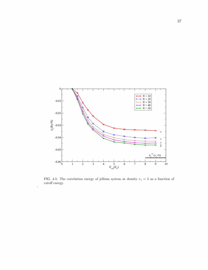
4.5 The correlation energy of jellium system at density rs = 5 as a func-
tion of cutoff energy. . . . . . . . . . . . . . . . . . . . . . . . . . . . 37
5.1 Finite size simulation cell for 3 types of systems. The top panel (a)
uses periodic boundary conditions for an isolated atomic or molecu-
lar calculation. The FS effect arises from spurious interactions of a
molecule with its own images. The middle panel (b) shows the model
for jellium. Jellium with a certain density rs is modeled with a sim-
ulation cell of any volume Ω containing N electrons where Ω and N
are chosen so that 4πr3s/3 = Ω/N . The bottom panel (c) illustrates
periodic boundary conditions applied in simulations of a solid. All
images of an electron are correlated to the electron in the simulation
cell. The size of the simulation cell that can be used in calculations
is discrete; being an integer multiple of the primitive cell. . . . . . . 40
xi

5.2 The size dependence of silicon bulk with respect to the system size.
Tabulated DMC data is provided by courtesy of Paul Kent (similar
to Fig. 2 and 4 in Ref. [47]). The largest cell with size of n = 5,
corresponding to Na = 250 atoms is assumed to be the infinite-size
limit. The DMC energies approach the infinite-size limit from below,
while the LDA energies approach it from above. The LDA corrected
DMC energies are seen to have larger FS errors. . . . . . . . . . . . . 43
5.3 The parameters B1(rs) and B2(rs). The data is taken from Kwon,
Ceperley and Martin’s DMC calculations [57]. . . . . . . . . . . . . . 46
5.4 The size dependence of jellium energies within the HF method. The
top figure shows the size dependence of the kinetic energy. ∆t(N)
is an oscillatory function with an envelop that decays as 1/N . The
lower figure shows the size dependence of the potential energy. ∆v(N)
decays smoothly as 1/N2/3. Both ∆t(N) and ∆v(N) are obtained
from averaging over many k-points. . . . . . . . . . . . . . . . . . . . 50
5.5 Comparison of the QMC, extrapolation (Eq. (5.4)), and fitting func-
tion (see Table. 5.2) for jellium system inside cubic boxes of size
L=7.533 Bohr up to 10.259 Bohr. . . . . . . . . . . . . . . . . . . . . 53
5.6 Comparison of the QMC, extrapolation (Eq. (5.4)), and fitting func-
tion (see Table. 5.2) for jellium system inside cubic boxes of size
L=10.722 Bohr up to 18.000 Bohr. . . . . . . . . . . . . . . . . . . . 54
5.7 Comparison of g(rs) obtained from extrapolation and QMC calcula-
tions. The extrapolation values are only accurate for large number of
particles, as indicated by good agreement between QMC values and
extrapolation values. For small number of particles, QMC values of
g(rs) differ from the extrapolation curve, which break down. . . . . . 55
5.8 The FS exchange and correlation energy per particles for several sim-
ulation cell sizes. The top figure shows the exchange energy per
particle. The dashed line represents the choice in the low density
(rs < R2) region for atomic/molecular system [Eq. (5.22)]; R2 visual-
ized by discontinuity, which moves to lower densities with increasing
L. In crystalline systems, the contribution from rs > R2 is negligible
for any reasonable size L, and we use a constant Ex(R2, L) to make
Ex continuous. The dot-dashed line represents the choice for solids.
The bottom figure show the correlation energy per particle. Note the
change of scale. . . . . . . . . . . . . . . . . . . . . . . . . . . . . . . 58
xii
6.1 The QMC, DFT and difference (QMC-DFT) energies of sodium (left
panels) and silicon (right panels) bulk. The sodium calculations are
done with 16 atom supercells using 50 random k-points. The silicon
calculations are done with 8 atom supercells using 5 k-points. There
are 3 lattice constants in each plot, expressed in terms of the experi-
mental lattice constant L0. Notice the change of scale in the bottom
panels. . . . . . . . . . . . . . . . . . . . . . . . . . . . . . . . . . . . 61
6.2 Alternative correction for one-body FS error. The top panel shows the
QMC energies of 16 atom supercells for bcc Na after the corrections
using Eq. (6.2), the bottom panel shows the QMC energies after the
corrections using Eq. (6.3). Each panel shows results for three lattice
constants. The value of a(Ω) varies from 1.17 to 1.33. The energy
fluctuations using the alternative correction method in bottom figure
are smaller than in the top figure. . . . . . . . . . . . . . . . . . . . . 63
6.3 The energies of DFT (top panel) and FS DFT (middle panel) cal-
culated for 50 random k-points. The 3 curves in each panel are the
energies for 3 lattice constants. The bottom panel shows the two-
body FS correction, as defined in Eq. (6.4). . . . . . . . . . . . . . . . 64
6.4 The QMC energy of the P2 molecule using supercells and periodic
boundary condition. The dashed and dotted lines are the DFT en-
ergies calculated with the infinite-size XC function and the FS XC
function, respectively. The blue solid line with circles is the QMC
energy. The the dashed line with boxes and the dotted lines with
diamonds are the QMC energy after correction with the infinite-size
limit and FS DFT XC function, respectively. The inset shows the
same energy plotted with respect to 1/Ω. . . . . . . . . . . . . . . . 66
6.5 Total energy per atom of silicon as a function of simulation cell size n.
The vertical axis is defined as ∆E ≡ E(Na)−E∞. The black circles
represent the raw energies (DMC), the one-body corrected energies
are given by red squares. The fully corrected energies are shown
by blue triangles. MPC energies, calculated by Kent et al. [47], are
shown as the green diamonds. The inset show the volume dependence
of two-body FS error. Both cubic and fcc results lie on the same linear
curve. . . . . . . . . . . . . . . . . . . . . . . . . . . . . . . . . . . . 70
xiii

6.6 The silicon atom total energy for simulation cell of sizes (14 Bohr)3
to (20 Bohr)3. The FS correction can not be applied to this atom be-
cause silicon atom has a spin polarization due to two spin up electrons
at orbital 2p. The infinite-size limit is obtained through extrapolation. 71
6.7 Convergence of the total energy of an 8 atom Si supercell for 3 lattice
constants, calculated using DFT (left panel) and QMC (right panel).
At Ecut = 25 Ry, the energy has already reached convergence. . . . . 72
6.8 Trotter error for 8 atom supercell of silicon bulk for 3 lattice con-
stants. Rydberg atomic unit is used in this figure. The production
calculations are done using ∆τ = 0.01. . . . . . . . . . . . . . . . . . 73
6.9 The energy of fcc silicon bulk as a function of lattice constant. The
calculations are done using 8 atom cubical supercell. The solid black
arrows indicate the positions of the equilibrium lattice constant for
different methods of calculations. The QMC energies (black circles)
and QMC + ∆E1−b energies (red boxes) are almost identical, as also
indicated by the size of one-body ∆E1−b FS correction in lower panel. 74
6.10 The sodium atom total energy for simulation cell of sizes (24 Bohr)3 to
(50 Bohr)3. These QMC energies do not have Monte Carlo statistical
error. The infinite-size limit is obtained through extrapolation. . . . . 77
6.11 top: Total energy per atom for bcc sodium bulk. The black line and
dashed line are the one-body-corrected and full-corrected energy per
atom of sodium simulations using 16 atoms. The red line and dashed-
dotted line are for the 54 atoms. The arrows indicate positions of
equilibrium lattice constants. bottom: the one-body and two-body
correction as a function of lattice constant. . . . . . . . . . . . . . . . 79
6.12 The ABO3 perovskite structure. Off-centering along the [0 0 1] axis
gives a tetragonal structure, while the off-centering along the diagonal
[1 1 1] yields a rhombohedral structure. . . . . . . . . . . . . . . . . . 82
6.13 The tetragonal and rhombohedral ferroelectric instabilities of per-
ovskite BiScO3 calculated with ABINIT using OPIUM pseudopoten-
tials. The positive x axis represent the distortion amplitude along
the [0 0 1] direction, while the negative x axis shows that along the
[1 1 1] direction. . . . . . . . . . . . . . . . . . . . . . . . . . . . . . . 83
xiv

6.14 The two-body FS corrections for two perovskite structures: tetrago-
nal and rhombohedral as a function of system sizes n. The corrections
are given in eV per primitive unit cells. The numbers of atoms (5n3)
for each system sizes are Na = 5, 40, 135 and 320. Inset: the two-body
FS correction as a function of 1/Na . . . . . . . . . . . . . . . . . . . 86
xv

CORRECTION OF FINITE SIZE ERRORS IN MANY-BODY ELECTRONIC
STRUCTURE CALCULATIONS

CHAPTER 1
Introduction
In today’s world, almost everyone uses electronic devices whose development is
based on our knowledge about the microscopic structure of materials. As science
develops, deeper understanding of electronic structure of material drives material
designs as major needs of human beings. The behavior of electronic devices, ranging
from simple resistors to complicated integrated circuits, depends on the structure
of atoms bound together by electromagnetic interactions governed by quantum me-
chanics (QM).
In QM, the evolution of a system is described by the Schrodinger equation,
whose Hamiltonian consists of one-body terms and two-body terms. One-body terms
such as kinetic energy of electrons and electron-ion interaction are easy to deal with,
while two-body terms arising from electron-electron interaction are difficult.
The Hartree-Fock (HF) theory and the density-functional theory (DFT) are
two important methods that are used to model the electron-electron interactions.
Both methods treat the electron-electron interaction as a collection of independent
electrons moving in self-consistent fields. These approaches are known as mean-field
approximations. HF theory is an approximate theory by construction, so it only
2
3
gives accurate results for certain systems. On the other hand, DFT is an exact
theory. However in its applications, certain approximations are incorporated into
calculations which limit its accuracy.
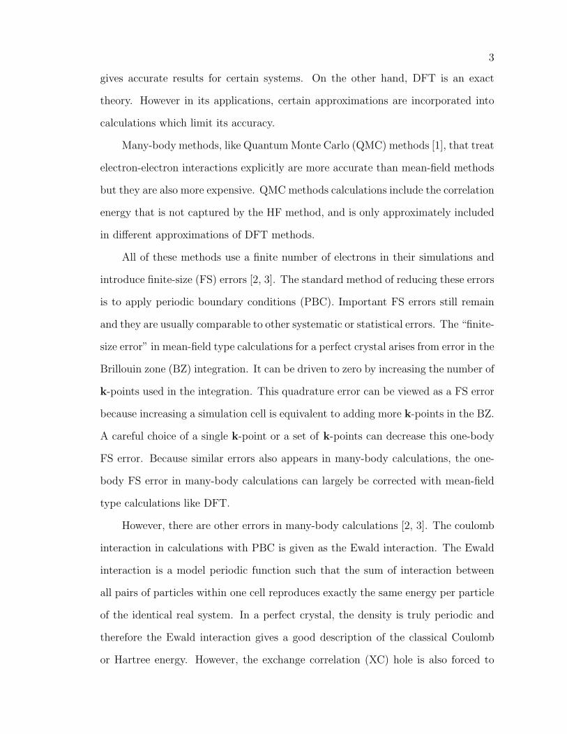
Many-body methods, like Quantum Monte Carlo (QMC) methods [1], that treat
electron-electron interactions explicitly are more accurate than mean-field methods
but they are also more expensive. QMC methods calculations include the correlation
energy that is not captured by the HF method, and is only approximately included
in different approximations of DFT methods.
All of these methods use a finite number of electrons in their simulations and
introduce finite-size (FS) errors [2, 3]. The standard method of reducing these errors
is to apply periodic boundary conditions (PBC). Important FS errors still remain
and they are usually comparable to other systematic or statistical errors. The “finite-
size error” in mean-field type calculations for a perfect crystal arises from error in the
Brillouin zone (BZ) integration. It can be driven to zero by increasing the number of
k-points used in the integration. This quadrature error can be viewed as a FS error
because increasing a simulation cell is equivalent to adding more k-points in the BZ.
A careful choice of a single k-point or a set of k-points can decrease this one-body
FS error. Because similar errors also appears in many-body calculations, the one-
body FS error in many-body calculations can largely be corrected with mean-field
type calculations like DFT.
However, there are other errors in many-body calculations [2, 3]. The coulomb
interaction in calculations with PBC is given as the Ewald interaction. The Ewald
interaction is a model periodic function such that the sum of interaction between
all pairs of particles within one cell reproduces exactly the same energy per particle
of the identical real system. In a perfect crystal, the density is truly periodic and
therefore the Ewald interaction gives a good description of the classical Coulomb
or Hartree energy. However, the exchange correlation (XC) hole is also forced to
4
be periodic in simulations with PBC. This unphysical approximation is particularly
inaccurate when the simulation cell is small. This two-body FS error is more difficult
to correct. Kohn-Sham DFT calculations do not have this error, since the XC energy
is evaluated using standard functional that has been extrapolated to the infinite-size
limit. Therefore, the conventional DFT calculations cannot be used as a correction
of the two-body FS error in many-body method calculations.
In this thesis, I report studies of these FS corrections [3]. The one-body FS error
can be corrected with conventional DFT methods and it is a well-known correction in
solid state calculations. We construct a new finite-size-DFT that is used to estimate
the two-body FS error. This new FS DFT uses a FS exchange-correlation function
to approximately include the two-body FS error in DFT calculations. Applications
of the method to the P2 molecule (in supercells with periodic boundary conditions),
to semiconductor bulk silicon, to sodium metal and to perovskite BiScO3 indicates
that the methods remove most of the FS errors, accelerating convergence toward
results for the infinite-size system.
The rest of this thesis is organized as follows.
In Chapter 2, I give a summary of several electronic structure methods. The
objective of the chapter is to provide a general overview of the many-body problem
and the methods for its approximate solutions like Hartree-Fock (HF) and density
functional theory (DFT). Many-body methods like configuration interaction (CI)
and quantum Monte Carlo (QMC) are briefly discussed.
In Chapter 3, I review the auxiliary field Quantum Monte Carlo (AFQMC)
method. This method is used to obtain all many-body results in this thesis. Here, I
discuss its use with a planewave basis and also the formalism of the second-quantized
form of the many-body Hamiltonian. Review of the ground state projection is also
covered in this chapter.
In Chapter 4, I present one simple application of the AFQMC method to the

5
interacting electron gas (jellium) system. Jellium calculations are used to construct
the finite-size exchange-correlation function. The HF solution of infinite-size jellium
system is discussed here together with the definition of the correlation energy. I also
present calculations on the cutoff energy dependence of the jellium correlation en-
ergy. The details data of this cutoff energy dependence are reported in Appendix B.
In Chapter 5, I construct finite-size exchange-correlation function based on a
fit to the jellium results. Existing correction schemes are also discussed.
In Chapter 6, I present several applications of the new correction schemes. The
first application is the size convergence study of the energy of the P2 molecule, using
supercells and periodic boundary conditions. While the uncorrected QMC energy
converges slowly to the infinite-size limit, the new corrections improve the energy
convergence significantly. The second application is to fcc silicon, where corrections
are applied to previously obtained results for silicon supercells. The results show
that our corrections are better than existing methods, and greatly improve size con-
vergence. The next application is to metallic bcc sodium. Many QMC calculations,
each with different k-point, are used to address the “open shell” problem in metallic
calculations. The corrected cohesive energies are in excellent agreement with the
experimental value. The last application is to well-depth calculations of BiScO3
perovskite. The corrected well-depths of QMC are in good agreement with the well-
depths calculated with the DFT method, indicating that the DFT well-depths are
reliable.
Chapter 7 summarizes our results and comments on the future prospects of this
research.
CHAPTER 2
Electronic Structure Methods
2.1 Introduction
The non-relativistic time-independent Schrodinger equation is given by
H|Ψ〉 = E|Ψ〉, (2.1)
where H is the Hamiltonian operator for a system of nuclei and electrons at positions
dα and ri, respectively. In Hartree atomic units, the Hamiltonian for N electrons
and Na nuclei is
H = −1
2
N∑i=1
∇2i −
Na∑α=1
1
2Mα
∇2α −
N∑i=1
Na∑α=1
Zα|ri − dα|
+1
2
N∑i=1
N∑j 6=i
1
rij+
1
2
Na∑α=1
Na∑β 6=α
ZαZβdαβ
,
(2.2)
where Mα is the mass of nucleus α, and Zα is the atomic number of nucleus α.
The first term in right hand side of Eq. (2.2) is the operator for kinetic energy of
the electrons; the second term is the operator for kinetic energy of the nuclei; the
third term represents the interaction between the nuclei and electrons; the fourth
and the fifth terms represent the repulsion between electrons and between nuclei,
6

7
respectively. The factor one half in the last two terms is needed to compensate the
double counting of the sum.
Fig. 2.1 illustrates this configuration. The distance between the i-th electron
and α-th nucleus is |ri − dα|; the distance between the i-th and j-th electron is
rij = |ri − rj|; and the distance between the α-th nucleus and the β-th nucleus is
dαβ = |dα − dβ|.
FIG. 2.1: Illustration of a quantum mechanical system. The positions of Nuclei and elec-trons are shown by vector position dα and ri, respectively. i, j are indexes for electronsand α, β are indexes for nuclei.
Since the nuclei are much heavier than electrons, they move much more slowly,
hence, to a good approximation, one can neglect the kinetic energy of these nu-
clei. This is the Born-Oppenheimer approximation [4]. Using the approximation,
Eq. (2.2) is simplified to an electronic hamiltonian:
H = −1
2
N∑i=1
∇2i −
N∑i=1
Na∑α=1
Zα|ri − dα|
+1
2
N∑i=1
N∑j 6=i
1
rij. (2.3)
8
Within this approximation, the last term in Eq. (2.2) becomes a constant, and
therefore it does not have effect on the electronic eigenstate. This ion-ion interaction
will be added to the eigenenergy of Eq. (2.3) to obtain the total energy of the
system. The Schrodinger equation for the wave function, Ψ(r1s1, r2s2, . . . , rNsN),
of N electrons subject to the ionic potential of Na nuclei is given by
N∑i=1
(−1
2∇2iΨ−
Na∑α=1
Zα|ri − dα|
Ψ
)+
1
2
N∑i,ji 6=j
1
|ri − rj|Ψ = EΨ. (2.4)
This 3N -dimensional partial differential equation is exactly solved only for system
with N = Na = 1, that is the system of a hydrogen atom.
In this thesis, I use two types of atomic units: Hartree atomic units and Rydberg
atomic units. In Hartree units, the universal constants are defined as 4πε0 = me =
e = ~ = 1, while Rydberg units, they are defined as 4πε0 = 2me = e2/2 = ~ = 1.
The Bohr radius a0 is the unit for length in both units. In Rydberg units, a unit
of energy 1 Ry is equal to 13.6056923 eV, while in Hartree units, a unit of energy 1
Ha is equal to 27.2113845 eV.
2.2 Mean-field Type Methods
2.2.1 Hartree-Fock Method
The Hartree-Fock (HF) method [5] approximately solves Eq. (2.4) by restricting
the wave function to a single N × N determinant, known as a Slater determinant,
where N is number of electrons. By construction, a Slater determinant satisfies the
Pauli principle. A Slater determinant of N electrons with positions ri and spins si
occupying N orbital is given by:

9
Ψ(r1s1, r2s2, . . . , rNsN) =1√N !
∣∣∣∣∣∣∣∣∣∣∣∣∣
χ1(r1s1) χ1(r2s2) . . . χ1(rNsN)
χ2(r1s1) χ2(r2s2) . . . χ2(rNsN)
......
...
χN(r1s1) χN(r2s2) . . . χN(rNsN)
∣∣∣∣∣∣∣∣∣∣∣∣∣, (2.5)
where a single particle wavefunction χi(rjsj) is given by the product of a spatial
part ϕ(rj) and a spin part η(sj), i.e. χi(rjsj) = ϕi(rj)ηi(sj).
The expectation value of the Hamiltonian with respect to this wave function is
given by
〈Ψ|H|Ψ〉 =∑i
∫drϕ∗i (r)
(−1
2∇2 + Vion(r)
)ϕi(r)
+1
2
∑i,j
∫drdr′
1
|r− r′||ϕi(r)|2|ϕj(r′)|2
− 1
2
∑i,j
∫drdr′
1
|r− r′|δsi,sjϕ
∗i (r)ϕi(r
′)ϕ∗j(r′)ϕj(r),
(2.6)
where the orthogonal properties of the spin function ηi(sj) has been used to obtain
this equation. The first and second terms are the kinetic energy and the ionic po-
tential energy, respectively. The third and fourth terms are known as the Hartree
energy and the exchange energy, both arising from the electron-electron interaction.
The antisymmetric property of the wave function gives rise to the exchange term.
This term lowers the total energy and physically expresses the Pauli exclusion prin-
ciple that electrons with same spins may not share the same spatial wave function.
Note that the spin dependence only appears in the last term.
Minimizing Eq. (2.6) with respect to the ϕi leads to the HF equations:
−1
2∇2ϕi(r) + Vion(r)ϕi(r) + VH(r)ϕi(r) +
∫vx(r, r
′)ϕi(r′)dr′ = εiϕi(r), (2.7)
where Vion(r), VH(r) and vx(r, r′) are ionic, Hartree and non-local exchange poten-

10
tial, respectively,
Vion(r) = −Na∑α=1
Zα|r−Rα|
, (2.8)
VH(r) =∑j
∫dr′|ϕj(r′)|2
|r− r′|, (2.9)
and
vx(r, r′) = −
∑j
1
|r− r′|ϕ∗j(r
′)ϕj(r)δsisj . (2.10)
Eq. (2.7) is solved self-consistently. A guess is made for each ϕi to determinant
VH(r) and vx(r, r′) and the differential equation is solved for the new ϕi, repeated
the processes iteratively until self-consistency is reached.
The final solution to the Hartree Fock equations is a set of orthonormal HF
spin orbitals χi with orbital eigenenergies εi. In the ground state configuration,
the N spin orbitals with lowest eigenenergies are occupied. The total number of
spin orbitals, occupied and unoccupied spin orbitals, is given by the number of
basis functions M , where M must be larger or equal to N , the number of electrons.
Using larger number of basis functions M decreases the ground state energy which
according to the variational principle, improves the HF ground state. The limit of
this improvement is known as the Hartree-Fock limit.
The HF energy can be improved by adding more Slater determinants to lower
the total energy of the system. At the limit of an infinite number of Slater deter-
minants, the exact ground state energy is obtained. The difference between this
exact ground state energy and the Hartree-Fock ground state energy is known as
the correlation energy.
2.2.2 Density Functional Theory
Density functional theory (DFT) approaches the many-body problem from a
different direction than HF theory, and includes correlation approximately [6, 7].

11
Kohn and Sham [8] introduced the idea of an auxiliary noninteracting system with
the same density as the real system. This enabled them to express the electron
density of the interacting system in terms of the one-electron wave functions of the
noninteracting system,
n(r) =N∑i=1
|ϕi(r)|2, (2.11)
and to write the Hohenberg-Kohn energy functional [6] in the form
E[n(r)] = −1
2
N∑i=1
∫drϕ∗i (r)∇2ϕi(r) +
∫drn(r)Vion(r)
+1
2
∫drdr′
n(r)n(r′)
|r− r′|+ Exc[n(r)],
(2.12)
where the terms on the right-hand side are the kinetic energy of the noninteracting
system with electron density n(r), the energy of interaction with the ionic potential,
the Hartree energy, and the exchange-correlation energy. Eq. (2.12) can be taken
as the definition of the exchange-correlation energy functional Exc[n(r)]. It can be
proved [6–8] that if the exact universal functional Exc[n(r)] were known, the density
that gives the global minimum of the energy in Eq. (2.12) is the ground state density
while the energy is the ground state energy. Unfortunately, this function is not
known exactly and has to be approximated.
Minimization of Eq. (2.12) with respect to the ϕi(r) gives rise to the self-
consistent Kohn-Sham equation,(−1
2∇2 + Vion(r) + VH(r) + Vxc(r)
)ϕi(r) = εiϕi(r), (2.13)
where the Hartree potential is
VH(r) =
∫n(r′)
|r− r′|, (2.14)
and the exchange-correlation potential is given by the functional derivative
Vxc(r) =δExc[n(r)]
δn(r). (2.15)

12
This self-consistent equation can be solved iteratively after one chooses an approxi-
mation to the exchange-correlation energy.
The simplest and best-known approximation for Exc[n(r)] is the local-density
approximation (LDA),
ELDAxc [n(r)] =
∫Egasxc (n(r))n(r)dr, (2.16)
where Egasxc (n) is the exchange-correlation energy per electron in a uniform interacting
electron gas of density n calculated using quantum Monte Carlo simulations [9, 10].
The superscript “gas” is used to emphasize that the exchange-correlation energy is
obtained from interacting electron gas calculations. This superscript will be removed
later. LDA treats the non-uniform electron density at r as if it were part of a uniform
electron gas of constant density n = n(r). This approximation is obviously accurate
for a system that has almost uniform density. However even on systems with a
strongly inhomogeneous density, applications of LDA work surprisingly well.
Finding better approximations to Exc is an area of active research today. For
further discussion, see Refs. [4] and [11].
2.3 Many-body methods
2.3.1 Configuration Interaction
There are numerous many-body methods, and this section focuses on configu-
ration interaction (CI) type methods because they bear a formal relationship to the
quantum Monte Carlo (QMC) method used in this thesis. Both methods are based
on representation of the many-body wave-function by Slater determinants.
Hartree-Fock theory oversimplifies the many-body problem, restricting the Hil-
bert space of many-body wave functions to single Slater determinants. One obvious
13
improvement of this method is to enlarge the Hilbert space to multi Slater deter-
minant space. One can include the HF single Slater determinant ground state and
the excited configurations created from this ground state. The ground state and all
the excited configurations are orthogonal to each other. This approach is known as
configuration interaction (CI). It is exact in the limit for a given basis.
In practice, one needs to truncate the infinite number of single-particle basis
set that constructs the single Slater determinant to a reasonable finite number of
single-particle basis set M (M includes both spatial and spin basis set). Using this
truncated basis set, one constructs a single Slater determinant and then creates all
the excited states determinants from it. For N electrons, using M basis functions,
one needs M !N !(M−N)!
determinants. This procedure, called full CI, is the standard in
quantum chemistry to benchmark the accuracy of other methods in small system
size calculations.
Even for relatively small systems and minimal basis sets, the number of de-
terminants that must be included in a full CI calculation is extremely large. This
exponential wall [7] limits applications of full CI to small systems (N ≈ 20). Var-
ious approximations are introduced to the full CI matrix by truncating the full CI
expansion and use only a small fraction of the possible determinants, for example
singly and doubly excited CI (SDCI). Another approach to limit the CI expansion
is called the multiconfiguration self-consistent field (MCSCF) method. The basic
idea of this approach is to optimize not only the expansion coefficients of the Slater
determinant orbitals, but also orbitals as well. For a more detailed discussion see
Ref. [5].

14
2.3.2 Quantum Monte Carlo
The Hartree-Fock method neglects electron correlation completely. To include
correlation terms, one needs to use a multi determinant space which leads to con-
figuration interaction. However, one will encounter the exponential wall that limits
the size of the system that can be simulated. On the other hand, density functional
theory includes correlations in an approximate functional. It works well in many
cases, but in several properties, one need to get accurate correlation energies.
Quantum Monte Carlo (QMC) methods offer a promising alternative [1]. QMC
treats the electron-electron interaction exactly. Its required computer time scales
algebraically [12] (as opposed to exponentially in CI) with system size. Rather than
explicitly integrating over phase space, Monte Carlo methods sample it.
The first and simplest many-body calculation that employs Monte Carlo tech-
niques is the variational Monte Carlo (VMC) method [13]. As indicated by its name,
it optimizes a trial wavefunction to obtain a variational estimate of the ground state
EV =
∫Ψ∗T (R)HΨT (R)dR∫Ψ∗T (R)ΨT (R)dR
≥ E0, (2.17)
where ΨT (R) is a trial wavefunction, H is the Hamiltonian of the system and E0
is the ground state energy. This 3N dimensional integral is calculated using the
Metropolis Monte Carlo method. Eq. (2.17) is rewritten in the form
EV =
∫|ΨT (R)|2[ΨT (R)−1HΨT (R)]dR∫
|ΨT (R)|2dR, (2.18)
and the Metropolis algorithm is used to sample a set of point Rm : m = 1,M
from the configuration-space probability density P(R) = |ΨT (R)|2/∫|ΨT (R)|2dR.
At each of these points the “local energy” EL(R) = ΨT (R)−1HΨT (R) is evaluated

15
and the average energy accumulated:
EV =1
M
M∑m=1
EL(Rm). (2.19)
The wave function consists of a product of Slater determinant and a Jastrow factor,
which enforces exact cups conditions [13].
More accurate quantum Monte Carlo methods are based on projection of the
ground state |ΨG〉 of a many-body Hamiltonian H from any known trial wave func-
tion |ΨT 〉 that satisfies 〈ΨT |ΨG〉 6= 0,
|ΨG〉 ∝ limβ→∞
e−βH |ΨT 〉. (2.20)
Different types of QMC methods are distinguished by the way they carry out
this projection. Diffusion Monte Carlo (DMC) is based on the similiarity of the
imaginary-time many-body Schrodinger equation with the diffusion equation [1].
DMC simulations for fermion systems suffer from the fermion sign problem [14],
which arises from the antisymmetric properties of fermion wavefunction. The fixed
node approximation [1, 15] controls the problem, yielding the lowest energy for a
given many-body nodal surface of the trial wavefunction. Thus the energy is varia-
tional, i.e. it will never be lower than the true ground state energy, but the results
depend on the quality of the trial wavefunction’s nodal surface.
Other Monte Carlo methods such as path-integral QMC, and auxiliary-field
QMC may also be used to study interacting many-electron systems. AFQMC will
be discussed in more detail in Chapter 3. For a more detail review of DMC methods,
see Refs. [1] and [16].
CHAPTER 3
Auxiliary Field Quantum Monte
Carlo
The recently developed phaseless auxiliary field quantum Monte Carlo method
[17–25] provides an alternative to the DMC method. Like DMC, AFQMC projects
the ground state of a many-electron system from a trial wave function. The major
difference is the space where the projections work. While DMC methods sample
the many-body wave function in real space, AFQMC method samples it in Slater
determinant space. This automatically incorporates the antisymmetric requirement
of the fermionic wavefunction. AFQMC methods also have a different way to han-
dle the sign problem which has shown promise in reducing the dependence of the
systematic errors on the trial wave functions.
The orbitals written in the Slater determinant can be expressed in a variety
of single particle basis states (e.g. planewaves, Gaussians, etc.) which allows
AFQMC to share much of the same computational machinery with DFT and other
independent-particle type methods. AFQMC can thus straightforwardly incorporate
many of the methodological advances from mean-field methods (such as pseudopo-
16

17
tentials and fast Fourier transforms), while systematically improving on mean-field
accuracy.
Applications of the method using a planewave basis on a few simple systems
[17, 20, 25] as well as more correlated TiO and MnO molecules [23] yielded excellent
results. More systematic applications of the phaseless AFQMC method to atoms and
molecules have been carried out using Gaussian basis sets. All-electron calculations
for first-row systems [22] as well as effective-core potential calculations in post-d
group elements [21] show excellent agreement with near-exact quantum chemistry
results and/or experiment. At the large basis-size limit, the AFQMC results for both
types of basis sets are in good agreement with each other and with experimental
values [24].
In this thesis, I use a planewave basis set to calculate energies of different atoms,
molecules and solids. While the use of a localized basis set such as Gaussian is favor-
able for atomic/molecular systems, it is straightforward to implement the planewave
basis on an extended system with periodic boundary conditions. A planewave basis
set also has several other advantages. It provides an unbiased representation of the
wave function, since its convergence is determined by just a single parameter, the
planewave kinetic-energy cutoff Ecut. It is also algorithmically simple to implement
and can be made very efficient with fast Fourier transform techniques as in DFT
methods. The use of pseudopotentials to remove highly localized core electron states
keeps the planewave basis tractable.
3.1 Conventions
In this section, I introduce some conventions that will be used in all of this
chapter and also through out all of this thesis. These conventions follow closely the
conventions in Ref. [26] and is meant to be for general cases, but many examples

18
will be given for the AFQMC planewave basis code that was used in this thesis.
• N : number of total electrons. In more general cases, Nσ is a number of electrons
with spin σ (σ =↑ or ↓).
• M : number of single-electron basis states. In our case, this is the number of
planewaves that have kinetic energy lower than Ecut. Typically M Nα for
planewave.
• |χi〉: the ith single-particle basis (i = 1, 2, . . . , M). In our case, this will be
planewave basis.
• c†i and ci: creation and annihilation operators for an electron in state |χi〉, i.e.
〈r|c†i |0〉 = 1Ω1/2 e
i(k+Gi)·r. They satisfy the usual anticommutation relation
c†icj + cjc†i = δij, (3.1a)
c†ic†j + c†jc
†i = 0, (3.1b)
cicj + cjci = 0. (3.1c)
ni ≡ c†ici is the corresponding number operator.
• |ϕi〉: A single particle orbital is expressed as
|ϕi〉 =∑j
ϕj,i|χj〉. (3.2)
• |φ〉: An N -electron Slater determinant
|φ〉 =1
N !A|ϕ1ϕ2 . . . ϕN〉, (3.3)
where A is an antisymmetric operator.
• ϕ†i : orbital creator operator. It creates particles in ith orbital from M basis states
ϕ†i =M∑j
ϕj,ic†j. (3.4)

19
With this definition, a Slater determinant is given by
|φ〉 = ϕ†1ϕ†2 . . . ϕ
†N |0〉. (3.5)
• The N -particle Slater determinant is completely specified by the M ×N matrix
Φ:
Φ ≡
ϕ1,1 ϕ1,2 . . . ϕ1,N
ϕ2,1 ϕ2,2 . . . ϕ2,N
......
...
ϕM,1 ϕM,2 . . . ϕM,N
, (3.6)
where M is the number of basis functions. Each column of the matrix represents
an orbital.
• |Ψ〉 is a many-body wave function which is not necessarily a single Slater de-
terminant. In the AFQMC method, a many-body wave function is given as a
stochastic sum over many Slater determinants.
There are several properties of Slater determinants that are useful in applica-
tions [26].
• For any Slater determinants |φ〉 and |φ′〉, the overlap between them is given by
〈φ|φ′〉 = det(Φ†Φ′
). (3.7)
• An operation of any Slater determinant by any operator B of the form
B = exp
(∑ij
c†iUijcj
)(3.8)
will lead to another Slater determinant [27]:
B|φ〉 = φ′†1 φ′†2 . . . φ
′†N |0〉 ≡ |φ
′〉, (3.9)

20
with φ′†m =∑
j c†jϕ′jm and Φ′ ≡ eUΦ, where U is a square matrix whose elements
are given by Uij. Therefore B ≡ eU is also a square matrix of size M ×M . Al-
gebraically, the operation of B on |φ〉 is simply a matrix multiplication involving
matrix M ×M and matrix M ×N .
• The single-particle Green function Gij ≡ 〈c†icj〉 is given by [28]
Gij ≡〈φ|c†icj|φ′〉〈φ|φ′〉
=[Φ′(Φ†Φ′
)−1Φ†]ji. (3.10)
• The two-particle Green function Gijkl ≡ 〈c†ic†jckcl〉 is given by [25]
Gijkl ≡〈φ|c†ic
†jckcl|φ′〉〈φ|φ′〉
= GliGkj −GkiGlj. (3.11)
3.2 Planewave Basis
Periodic boundary conditions (PBC) are easily incorporated using a planewave
basis. According to Bloch’s theorem [29], every single particle electronic wave func-
tion in a periodic solid can be written as the product of a planewave times a function
with periodicity of the Bravais lattice:
ϕi(r) = eik.rui,k(r). (3.12)
A vector k determines a choice of one particular PBC of a system. A periodic
function can be expanded in a planewave basis whose wave vectors are reciprocal
lattice vector of the crystal:
ui,k(r) =∑G
ci,k+GeiG·R, (3.13)
where the reciprocal lattice vector G are defined by G.R = 2πm for all R in a
Bravais lattice defined by the simulation cell, and m is an integer. A simulation cell
21
of volume Ω can be a primitive cell or a supercell consists of several primitive cells.
Any single particle wave function given in the form of Eq. (3.12) can be written as
ϕi(r) =∑G
ci,k+Gei(G+k)·r, (3.14)
so that a planewave basis |k + G〉 is defined in real space as
〈r|k + G〉 ≡ 1√Ωei(k+G)·r. (3.15)
The orthogonality of conditions are given by
〈q|q′〉 =1
Ω
∫Ω
d3re−i(q′−q)·r = δq,q′ , (3.16)
and
〈r|r′〉 =1
Ω
∑q
eiq·(r−r′) = δ(r− r′), (3.17)
where q ≡ k + G here.
The planewave basis defined by Eq. (3.15) spans to infinity. This is not practical
for computer simulation. In practice, we will consider only G vectors whose kinetic
energies 12(k + G)2 are smaller than or equal to a given cutoff energy Ecut. This
defines the G-space that we will work in. Correspondingly, the real space is taken
to be the Fourier space of the G-space.
3.3 Hamiltonian
The hamiltonian within Born-Oppenheimer approximation is given by
H = K + Vei + Vee + Vii (3.18)
For a given k-point, the kinetic energy is given in the second quantized form by
[17, 25] :
K =1
2
∑G,λ
(k + G)2c†k+G,λck+G,λ, (3.19)

22
where λ is a spin of an electron.
The other terms are the Coulomb interaction terms. For system consists of Na
ions and N electrons, the total interactions are given by [2]
U =N∑i=1
Na∑α=1
Zαψ (ri,dα) +1
2
N∑i=1
N∑j=1j 6=i
ψ (ri, rj) +Nξ
2
+1
2
Na∑α=1
Na∑β=1β 6=α
ψ (dα,dβ) +ξ
2
Na∑α=1
Z2α.
(3.20)
where the interaction potential ψ(r, r′) is a modified Coulomb potential that in-
corporates the periodic boundary condition and ξ is the self-energy term. The
representation of this modified Coulomb potential in Fourier space is 1|G−G′|2 , which
is the same with the Fourier representation of the original Coulomb potential.
The first term in Eq. (3.20) is the electron-ion interaction. Here we use a norm
conserving LDA Kleinman-Bylander (KB) nonlocal pseudopotential [30, 31]. The
pseudopotential models the interaction between valence electrons and atomic core
(atomic nuclei and core electrons), so the number of electrons that are involved in
calculations is significantly reduced. In second quantized formalism, these pseu-
dopotentials can be written as
Vei =∑G,G′
V loc(G−G′)c†k+Gck+G′ +∑G,G′
V nl(k + G,k + G′)c†k+Gck+G′ , (3.21)
where V loc(G−G′) and V nl(k + G,k + G′) are the matrix element of local and
nonlocal potential as described in Appendix A. Now the local part can be rewritten
as follows:
V locei =
1
2
∑Q 6=0
V loc(Q)[ρ(Q) + ρ†(Q)] +NV loc(0), (3.22)
where N is the number of electrons. The last term is just a constant and it excludes
the Q = 0 divergent term coming from long range Coulomb interaction. The one-

23
body density operator ρ(Q) is given by
ρ(Q) ≡∑G,λ
c†k+G+Q,λck+G,λθ(Ecut − |k + G + Q|2/2
). (3.23)
The step function ensures that (k + G + Q) lies within planewave basis and the
summation over spin (λ = 1, 2) has been made explicit.
The second term in Eq. (3.20) is the electron-electron interaction. This term is
a two-body term. The matrix element is given by
〈k + Gi, λi; k + Gj, λj|V ee|k + Gk, λk; k + Gl, λl〉
= δλi,λkδλj ,λlδGi+Gj ,Gk+Gl
1
2Ω
4π
(Gi −Gk)2 . (3.24)
In second quantized formalism, the electron-electron interaction is given as
V ee =∑Gi,λi
′ ∑Gj ,λj
∑Gk,λk
∑Gl,λl
δλi,λkδλj ,λlδGi+Gj ,Gk+Gl
1
2Ω
4π
(Gi −Gk)2 c†k+Gi,λi
c†k+Gj ,λjck+Gl,λlck+Gk,λk . (3.25)
The primed summation indicates that the Gi = Gk singular term is excluded due
to charge neutrality. The change of variables
Gi = G + Q,
Gj = G′ −Q,
Gk = G,
Gl = G′,
(3.26)
guarantees that Gi+Gj = Gk+Gl. Using these new variables, Eq. (3.25) becomes
V ee =∑λi,λj
∑G,G′,QQ 6=0
1
2Ω
4π
Q2c†k+G+Q,λi
c†k+G′−Q,λjck+G′,λjck+G,λi . (3.27)
Using the commutation relations, Eq. (3.27) can be written as
V ee =∑λi,λj
∑G,G′,QQ 6=0
1
2Ω
4π
Q2c†k+G+Q,λi
ck+G,λic†k+G′−Q,λj
ck+G′,λj
− 1
2Ω
∑λi
∑G
∑Q 6=0
4π
Q2c†k+G,λi
ck+G,λi .
(3.28)

24
The first term can be simplified by using definition of ρ(Q) in Eq. (3.23). Note that
the sum over Q in second term has G dependence and therefore cannot be simplified
further. Let rewrite this term in original variable Q = Gi−Gk, and since Gi is just
a dummy index, this summation can be written as
V ee =1
2Ω
∑Q 6=0
4π
Q2ρ(Q)ρ†(Q)− 1
2Ω
∑λ
∑G,G′
G6=G′
4π
(G−G′)2c†k+G,λck+G,λ. (3.29)
If rearrangement of the terms in Eq. (3.28) is done differently, the electron-electron
terms can be written in the same form as Eq. (3.29) except that the term ρ(Q)ρ†(Q)
is flipped into ρ†(Q)ρ(Q).
The third term in Eq. (3.20) is the interaction term between electrons with their
own images. This constant Nξ2
term goes to zero as the simulation cell increases.
The fourth and fifth terms of Eq. (3.20) are the nuclei-nuclei interaction and nuclei
with they own images interaction, respectively. These terms are also constant.
In second quantization language, all terms in the Hamiltonian can be regrouped
into constants, one-body parts and two-body parts. The Hamiltonian is rewritten
as follow:
H = H(0) + H(1) + H(2) (3.30)
H(0) = NV loc(0) +1
2Nξ +
1
2
M∑α=1
M∑β=1β 6=α
ψ (dα,dβ) +ξ
2
M∑α=1
Z2α. (3.31)
H(1) =1
2
∑G,λ
(k + G)2c†k+G,λck+G,λ +1
2
∑Q6=0
V loc(Q)[ρ(Q) + ρ†(Q)]
+∑G,G′
V nl(k + G,k + G′)c†k+Gck+G′
− 1
2Ω
∑λ
∑G,G′
G 6=G′
4π
(G−G′)2c†k+G,λck+G,λ.
(3.32)

25
H(2) =1
2Ω
∑Q 6=0
4π
Q2ρ(Q)ρ†(Q). (3.33)
The two-body terms can be written in more symmetric way as follow:
H(2) =∑Q6=0
π
ΩQ2
[ρ(Q)ρ†(Q) + ρ†(Q)ρ(Q)
]. (3.34)
Hermitian operators A(Q) and B(Q) are defined as
A(Q) ≡√
2π
ΩQ2
[ρ(Q + ρ†(Q)
], (3.35)
B(Q) ≡ i
√2π
ΩQ2
[ρ(Q− ρ†(Q)
], (3.36)
so that the two-body operator can be written as a sum of quadratic operator:
H(2) =1
4
∑Q 6=0
[A2(Q) + B2(Q)
]. (3.37)
3.4 Ground-State Projection
The ground state |Ψ0〉 of a Hamiltonian H is obtained from an imaginary time
projection of a trial wave function |ΨT 〉:
limn→∞
(e−∆τ(H−E0)
)n|ΨT 〉 = |Ψ0〉, (3.38)
where E0 is an estimate of the lowest eigenenergy of Hamiltonian H. This projec-
tion works provided 〈ΨT |Ψ0〉 6= 0. In present applications, |ΨT 〉 is a single Slater
determinant obtained from a mean-field calculation, although including more Slater
determinants are sometimes used in other applications . With a choice of small ∆τ ,
it is safe to separate the one-body and the two-body terms in the Hamiltonian using
the Trotter-Suzuki decomposition [32, 33]:
exp(−∆τH) = exp(−∆τ [H1 + H2])
= exp(−1
2∆τH1) exp(∆τH2) exp(−1
2∆τH1) +O(∆τ 3),
(3.39)
26
where an error of order ∆τ 3 is introduced. As mentioned in Sec. 3.1, an applica-
tion of the one-body propagator exp(−12∆τH1) on a single Slater determinant |φ〉
leads to another single Slater determinant |φ′〉 = exp(−12∆τH1)|φ〉. The two-body
propagator in the form of square of one-body propagators can be transformed into
one-body propagator using the Hubbard-Stratonovich transformation [34, 35],
exp
(−1
2∆τ∑i
λib2i
)=
∫ (∏i
dσi√2π
)exp
[∑i
(−1
2σ2i + σi
√−∆τλibi
)].
(3.40)
This can be written more compactly as,
e−∆τH(2)
=
(1√2π
)dim(σ) ∫dσe−
12σ·σe
√∆τσ·v, (3.41)
where we introduce a vector σ ≡ σi, whose dimensionality dim(σ), is the number
of all possible Q-vectors satisfying Q = G−G′. Vectors G and G′ are the reciprocal
lattice vector whose kinetic energy smaller than Ecut. The operator v ≡ √−λibi
are given by the iA(Q) or iB(Q) one-body operator, since all the λi = 1 in the
planewave case.
In the original applications of the AFQMC method [36, 37], the multidimen-
sional integrations are calculated with a Metropolis algorithm. While in our AFQMC
simulation [14, 17, 26], we use importance-sampling transformation to turn the pro-
jection into a branching random walk in an over-complete Slater determinant space.
The important sampling improves the quality of the random walk by providing a
guidance for the walker based on the projected overlap with trial wave function.
More importantly, it also allows the imposition of a constraint to control the phase
problem.
The phase problem arises from the fact that the projection operators cannot be
made all real, or in other word the λi is not negative. As the random walk proceeds,

27
the orbitals
|φ′〉 ← exp(√
∆τσ · v)|φ〉 (3.42)
gain complex phases, which make the stochastic representation of the ground state
|Ψ0〉 become dominated by noise. This phase problem is similar to the well-known
sign problem [14], but it is more severe because, instead of +|φ〉 and−|φ〉 symmertry,
there are now an infinite set eiθ|φ〉, θ ∈ [0, 2φ), among which the Monte Carlo
sampling cannot distinguish.
The phaseless AFQMC method is used to control the phase problem in an ap-
proximate manner, using a trial wave function [17, 25]. The method uses a complex
importance sampling function, the overlap 〈ΦT |φ〉, to construct phaseless random
walkers, |φ〉/〈ΨT |φ〉. The ground state is then represented as a stochastic sum of
walkers
|Ψ0〉 =∑φ
wφ|φ〉〈ΨT |φ〉
, (3.43)
where wφ is a weight of phaseless walker,
wφ = exp
[−∆τ
〈ΨT |H|φ〉〈ΨT |φ〉
]≡ exp[−∆τEL(φ)], (3.44)
and EL(φ) is a local energy of a walker.
The ground state energy calculated within mixed estimate is given by
E0 =〈ΨT |H|Ψ0〉〈ΨT |Ψ0〉
= limβ→0
〈ΨT |He−βH |ΨT 〉〈ΨT |e−βH |ΨT 〉
. (3.45)
In the stochastic representation, the ground state energy is given by
EMC0 =
∑φwφEL(φ)∑
φwφ. (3.46)
Detail discussion on the implementation of the phaseless AFQMC can be found at
Refs. [17, 18, 22].

CHAPTER 4
Jellium
The homogeneous electron liquid1, known as jellium, is the simplest realistic
model of interacting electrons in extended systems, yet it can provide valuable in-
sights into more complex systems [4]. This discussion will be restricted to non-spin
polarized jellium.
The local density approximation (LDA) of density functional theory (DFT)
uses the exchange correlation energy of jellium to describe realistic systems. There
is no a priori reason to believe that this will work well [39] but many applications
show that, in fact, this is often a good approximation, except for systems where the
correlation energy plays an important role in the physical properties.
In the jellium model, interacting electrons are allowed to move in a non-responsive
uniform positive neutralizing background charge. The Hamiltonian of the N electron
system of volume Ω, with N/Ω = n is given by
H = −1
2
N∑i
∇2i +
[1
2
N∑i 6=j
1
|ri − rj|− 1
2
∫d3rd3r′
n2
|r− r′|
], (4.1)
1The term electron liquid is used to emphasize the electron-electron interaction, as opposed toelectron gas that used in the independent electron model [38]. Sometimes, the term interactingelectron gas or simply jellium are also used.
28

29
where Hartree atomic units (~ = me = e = 4πε0 = 1) are used, so that lengths are
given in unit of the Bohr radius a0. The last term arises from the interaction between
the electrons with the positive background and the self energy of the background
with itself and divergent long-wavelength Coulomb interaction terms eventually drop
out due to charge neutrality [40] as the volume Ω→∞.
The whole system is parametrized only by the density of the electrons, charac-
terized by the average separation rs of the electrons in the system :
4
3πr3
s
N
Ω= 1. (4.2)
It is useful to write equation (4.1) in terms of scaled coordinates r=r/rs, instead
of atomic units (where r is in unit of a0),
H =
(1
rs
)2∑i
[1
2∇2i +
1
2rs
(∑j 6=i
1
|ri − rj|− 3
4π
∫d3r
|r|
)]. (4.3)
Eq. (4.3) shows that in the high density limit (rs → 0) the kinetic energy term is
dominant while for the low density limit (rs → ∞) the potential energy term is
dominant.
In practice, calculations are performed on a finite-size simulation cell with a
finite number of electrons, incorporating periodic boundary conditions, keeping the
same density as the infinite system’s density. Properties of the infinite-size limit are
obtained through extrapolation [9, 41], which will be discussed in Chapter 5.
The chapter is organized as follows. First I will discuss Hartree-Fock (HF)
solutions to the infinite-size limit of jellium system and define the correlation energy.
Benchmark AFQMC calculations for several densities and numbers of electrons will
be discussed. Finally, I will discuss convergence with respect to the (planewave)
basis.
30
4.1 Hartree-Fock Solution to the Infinite-Size-Limit
of Jellium System
The HF equation for a jellium system is given by [29]
−1
2∇2ϕi(r)−
∑j
∫dr′
1
|r− r′|ϕ∗j(r
′)ϕi(r′)ϕj(r)δsisj = εiϕi(r). (4.4)
The solution to the equations is
ϕi(r) =
(eiki·r√
Ω
)× spin function, (4.5)
in which each wave vector less than Fermi momentum kF occurs twice in the Slater
determinant. The infinite-size limit Ω → ∞ will be taken at the end of the cal-
culations. The relation between number of electrons N , Fermi momentum kF and
simulation cell size Ω = L3 is given by
N = 243πk3
F(2πL
)3 . (4.6)
The factor of two is included to take into account the fact that each state is occupied
by spin up and spin down electrons. The relation between Fermi momentum and
density is
kF =
(9π
4
) 13 1
rs. (4.7)
The single particle eigenenergies of the system are given by
ε(k) =k2
2− 2
πkFF
(k
kF
), (4.8)
where
F (x) =1
2+
1− x2
4xln
∣∣∣∣1 + x
1− x
∣∣∣∣ . (4.9)
The first term is the kinetic energy term and the second term is the exchange term.
31
The total kinetic energy of a jellium system is simply given by a sum of electron
energy states for all lowest states up to the Fermi sphere k = kF ,
EK = 2∑k<kF
k2
2. (4.10)
In the limit Ω→∞, this summation can be evaluated as integral to obtain
E∞KN≡ E∞K =
3
10k2F
=3
5εF .
(4.11)
Similarly, the exchange energy is given by [29],
Ex = −kFπ
∑k<kF
[1 +
k2F − k2
2kkFln
∣∣∣∣kF + k
kF − k
∣∣∣∣] , (4.12)
and converting the sum into an integration, the exchange energy per particle is given
by
E∞xN≡ E∞x = − 3
4πkF . (4.13)
The total HF energy per particle is then given by
E∞HF (rs) ≡E∞HF (rs)
N
=3
10
(9π
4
) 23 1
r2s
− 3
4π
(9π
4
) 13 1
rs
=1.10495
r2s
− 0.458165
rs.
(4.14)
This energy could also be obtained using perturbation theory. In high density
(i.e., small rs/a0), the kinetic energy is the 0th order energy, and the exchange energy
is the 1st order energy correction. The remaining terms in the series are called the
correlation energy [40] which is defined as the energy difference between the true
total energy and the HF energy
E∞c (rs) = E∞(rs)− E∞HF (rs). (4.15)
32
The asymptotic expansion for correlation energy of high density jellium (rs 1) is
given by
E∞c (rs) =1
π2(1− ln(2)) ln(rs)− 0.048 + 0.0020rs ln(rs)− 0.0116rs. (4.16)
The first and second terms were calculated by Gell-Mann and Brueckner (1957) [42]
and the other two terms are from a fit by Perdew and Zunger (1981) [10] to diffusion
Monte Carlo results of Ceperley and Alder (1980) [9].
4.2 Several Simple AFQMC Test Calculations
In this section, we describe several preliminary AFQMC calculations of jel-
lium. AFQMC calculations will be used to monitor the accuracy of finite-size fits
to Ec(rs, L) in Chapter 5. Calculations were first performed on an unpolarized 14
electron closed shell (all degenerate states underneath the Fermi surface are filled)
system for rs = 4.0 (cubic box of size 15.54 Bohr).
Table 4.1 shows good agreement between our results and previous results [43,
44]. The highest cutoff energy Ecut of the plane wave basis used in my calculations
was 25 Ry. This accurately describes electron scattering due to correlation effects
(the HF Fermi energy EF ∼ 0.16 Ry). The momentum distribution of electrons
given in Ref. [45] is negligible for electron with E > 4EF . Calculations using the
smaller cutoff energy of 2 Ry ( ∼ 12EF ) give a similar result, consistent with our
expectations.
Next we benchmark systems with larger number of electrons for several densi-
ties. Table 4.2 shows the energy per particle of 54 electron systems with rs between
1 and 20. At each calculation we use cutoff energy about or larger than 12EF . The
results are compared with calculations using diffusion Monte Carlo [46], and they
are in good agreement. For rs = 20, there is the discrepancy of about 6%. This dis-

33
TABLE 4.1: Correlation energy per electron of jellium with number of electrons N =14. The average distance of the electrons rs is 4.0. The results are compared with otherAFQMC calculations (see Ref. [43] and also see discussion on Ref. [44]). All quantitiesare in Rydberg atomic unit.
Ecut E EcAFQMC 25.0 −2.262± 0.005 −0.0445± 0.0003AFQMC 2.0 −2.275± 0.004 −0.0454± 0.0003AFQMC from ref [43] 1.31 −2.27± 0.04 −0.045± 0.003AFQMC from ref [43] 1.96 −2.34± 0.06 −0.050± 0.004AFQMC from ref [44] ∼ 3 −2.28± 0.08 −0.046± 0.006GFMC from ref [43] −2.297± 0.006 −0.0470± 0.0004
TABLE 4.2: Energy per electron of jellium with number of electrons N = 54. L is thesize of the cubic box. The error of the calculation is given in the last digit. All quantitiesare in the Rydberg atomic unit
L rs Ecut EF AFQMC Energy DMC energy6.09 1 40.0 3.19 1.0591(2) 1.0597(1)30.46 5 4.0 0.128 -0.1546(4) -0.15810(1)60.93 10 0.4 3.19× 10⁻² -0.1057(6) -0.10888(1)121.86 20 0.1 7.98× 10⁻³ -0.0601(4) -0.06408(1)
crepancy might come from the fact that the basis that we used is not large enough
for this low density system. More careful and systematic studies are needed to
eliminate possible small errors (time-step, cutoff, etc) for an accurate and unbiased
comparison between AFQMC and DMC. However, this low density region is not
important in generating finite-size exchange-correlation functional, since AFQMC
jellium results will only be used as a guide in our parametrization, we will not pursue
such calculations at greater details.

34
4.3 Cutoff Energy Dependence of Jellium Corre-
lation Energy
As required by the Pauli exclusive principle, the number of basis functions has
to be at least equal to the number of electrons. Therefore the correlation energy is
zero when Ecut = EF . Figures 4.1 - 4.5 show the convergence with respect to Ecut
for the range 1 ≤ rs ≤ 5, most important in realistic systems. Appendix B tabulates
these results.
As Ecut increases, more of the correlation energy is captured, eventually con-
verging to a value Ec(rs, L), which depends only on the density and system size. As
seen in figures 4.1 - 4.5, for Ecut ∼ 9EF , the error in the correlation energy is smaller
than the statistical errors. As anticipating our finite-size fits, the open circles at the
end of each curve are the FS correlation energy obtained from the functional given
in Table 5.2. This will be further discussed in Chapter 5.
The first derivative in figures 4.1 - 4.5 is seen to decrease in the low cutoff
energy region. For example, the correlation energies for N = 10 (the red curves in
figures. 4.1 - 4.5) are seen to be curved down. Further studies indicate that this
behavior also occurs for larger N , but at even lower cutoff energies. This finite-
size effect decreases as the number of particles increases to infinity. In this limit,
the correlation energies are expected behave monotonously in both the value and
first derivative. It would be useful to construct correlation energy functional that
depends on cutoff energy in the infinite-size limit Ec(rs, Ecut). Such a functional
would be useful for obtaining a finite-basis correction on many-body calculations.
Further studies are needed to establish these corrections.

35
0 1 2 3 4 5 6 7 8 9 10E
cut(E
F)
-0.12
-0.1
-0.08
-0.06
-0.04
-0.02
0
ε c(Ry/
N)
N = 10N = 20N = 30N = 40N = 50
εc
∞ (r
s=1)
FIG. 4.1: The correlation energy of jellium system at density rs = 1 as a function ofcutoff energy.
.
0 1 2 3 4 5 6 7 8 9 10E
cut(E
F)
-0.1
-0.08
-0.06
-0.04
-0.02
0
ε c(Ry/
N)
N = 10N = 20N = 30N = 40N = 50
εc
∞ (r
s=2)
FIG. 4.2: The correlation energy of jellium system at density rs = 2 as a function ofcutoff energy
.

36
0 1 2 3 4 5 6 7 8 9 10E
cut(E
F)
-0.08
-0.06
-0.04
-0.02
0
ε c(Ry/
N)
N = 10N = 20N = 30N = 40N = 50
εc
∞ (r
s=3)
FIG. 4.3: The correlation energy of jellium system at density rs = 3 as a function ofcutoff energy.
.
0 1 2 3 4 5 6 7 8 9 10E
cut(E
F)
-0.07
-0.06
-0.05
-0.04
-0.03
-0.02
-0.01
0
ε c(Ry/
N)
N = 10N = 20N = 30N = 40N = 50
εc
∞ (r
s=4)
FIG. 4.4: The correlation energy of jellium system at density rs = 4 as a function ofcutoff energy.
.
37
0 1 2 3 4 5 6 7 8 9 10E
cut(E
F)
-0.06
-0.05
-0.04
-0.03
-0.02
-0.01
0
ε c(Ry/
N)
N = 10N = 20N = 30N = 40N = 50
εc
∞ (r
s=5)
FIG. 4.5: The correlation energy of jellium system at density rs = 5 as a function ofcutoff energy.
.

CHAPTER 5
Finite Size Effects
Realistic many-body calculations for extended systems are needed to accurately
treat systems where the otherwise successful density functional theory (DFT) ap-
proach fails. These include high-temperature superconductors, transition metal ox-
ides, and systems where accurate treatments of bond-breaking or bond-stretching
are required. Effective single-particle methods such as DFT or Hartree Fock (HF)
routinely exploit Bloch’s theorem in calculations for extended systems. In crystalline
materials, the cost of the calculations depends on the number of atoms in the peri-
odic simulation cell, and the macroscopic limit is achieved by a simple quadrature
in the Brillouin zone (BZ), using a finite number of k-points. Many-body methods
with explicit two-particle interactions cannot avail themselves of this simplification.
Instead calculations must be performed using increasingly larger simulation cells
(supercells), extrapolating the results to infinite size. Finite size (FS) corrections
from large one-body contributions (kinetic energy, Hartree energy, etc.), which arise
from the downfolding of k-points into the smaller supercell Brillouin zone, can be
easily incorporated using auxiliary HF or DFT supercell calculations, and these can
accelerate size convergence [47]. Residual finite-size (FS) errors in many state-of-
38
39
the-art many-body calculations are usually still large and often more significant than
other statistical and systematic errors. In this chapter, I introduce a new method
[3] that is specifically designed to approximately include two-body FS corrections
in DFT calculations, through the use of FS exchange correlation functions. These
corrections accelerate the size convergence and reduce the dependence on the size
of the simulation cell.
The origin of the FS error is first explained, followed by a discussion of existing
correction methods using DFT and HF. FS effects in jellium are discussed next,
reviewing the extrapolation to the infinite-size limit. A reverse engineered FS ex-
change correlation function is then generated and a parametrization for this FS XC
function is given.
5.1 Origin of Finite Size Errors
In mean-field type calculations, such as DFT, FS errors effectively arise from the
discrete quadratures used to approximate Brillouin-zone integrations. The infinite
limit can be obtained in two ways. The first and more efficient way is to increase
the number of k-points sampled in the BZ, using the primitive simulation cell.
In this method, the cost of the calculations grow linearly with the number of k-
points. The second way is to increase the size of the simulation cell using only
a single or small number of k-points. This method is more expensive, since it
increases both the number of particles and the number of basis functions needed.
In many-body calculations, the infinite-size limit can only be achieved using the
second approach. Typically several many-body calculations, each at different k-
point, representing a particular choice of periodic boundary conditions (PBC) [see
Eq. (3.12)], are averaged to further reduce size effects.
The nature of the FS errors in many-body calculations is different from mean-

40
FIG. 5.1: Finite size simulation cell for 3 types of systems. The top panel (a) usesperiodic boundary conditions for an isolated atomic or molecular calculation. The FSeffect arises from spurious interactions of a molecule with its own images. The middlepanel (b) shows the model for jellium. Jellium with a certain density rs is modeled witha simulation cell of any volume Ω containing N electrons where Ω and N are chosenso that 4πr3s/3 = Ω/N . The bottom panel (c) illustrates periodic boundary conditionsapplied in simulations of a solid. All images of an electron are correlated to the electronin the simulation cell. The size of the simulation cell that can be used in calculations isdiscrete; being an integer multiple of the primitive cell.

41
field type calculations. Using DFT calculations to estimate the many-body FS errors
does not eliminate all of the FS error. In many-body calculations the long range
Coulomb interaction induces correlations between electrons at large distances and
these are not captured at the mean field level. Fully reproducing these long range
interactions requires large simulation cells. FS simulation cells in PBC effectively
use a modified form of the interaction which introduces errors.
Fig. 5.1 illustrates this FS error in three different types of systems.
a. FS errors in atomic/molecular systems with PBC:
It is sometimes convenient to model an isolated atom or molecule using PBC. As
a result, interactions with fake images are present. Increasing the simulation cell
size eventually removes this error. The cost of increasing the size of the supercell
in this atomic/molecular system is lower than for the solid, since only the size of
the basis increases, while the number of particles remains constant.
b. FS errors in jellium:
Jellium consists of electrons with uniform density n in the presence of a classical
constant positive background. In a simulation with PBC, this system is modeled
with a fixed number of electron N in a simulation cell of volume Ω, such that
N/Ω = n. As the number of N and volume Ω increases, the system approaches
the infinite-size limit. As in the case of solids, increasing the size of simulation
cell also increases both the number of particles and the number of basis functions.
By definition, the DFT energy of infinite jellium is exactly equal to the many-
body value for the infinite size system. We wish to construct a FS DFT exchange
correlation function that is equal to the many-body function for finite-size jellium.
c. FS error in solids:
In simulations with PBC, artificial periodicity is enforced on the many-body wave
function, which introduces FS errors.
42
5.2 Existing Correction Methods
The XC energy density Exc(n) of DFT is most often obtained from interpolation,
over a range of densities n, of quantum Monte Carlo (QMC) calculations of the
homogeneous interacting electron gas [9, 10, 41]. A key point is that the QMC
results, which are obtained with PBC, have been extrapolated to infinite supercell
size for each density n. This is the correct choice for DFT applications to extended
systems, where Bloch’s theorem will be used to reach infinite system size.
This choice is not ideal, however, if one seeks to obtain FS corrections from
the LDA. Fig. 5.2 shows the FS error for fcc bulk silicon calculated with diffusion
Monte Carlo (DMC) [47], LDA and with DMC corrected by LDA. The system size
for n=1 to 5 corresponds to Nion = 2, 16, 54, 128 and 250 atoms, respectively. The
FS error is determined by assuming that the largest system n = 5 is at the infinite-
size limit. All the calculations were done using a single k-point, the L-point in the
fcc BZ [48, 49]. The DMC energy is seen to have a different size dependence than
the LDA. DMC approaches the infinite-size limit from below, while the LDA energy
approaches from above. The size effect actually increases for LDA-corrected DMC.
FS errors can be separated into one-body and two-body FS errors. Sometimes
these errors are referred to as the independent-particle finite size error and the
Coulomb finite-size error [47], respectively. The one-body FS error is controlled by
k-point convergence and is also present in LDA calculations. As mentioned, these
errors are quadrature errors and can be systematically reduced by using more k-
points in the BZ integration [50]. The use of certain quadrature grids can accelerate
this convergence (so-called special k-point grid [51]), and the same is true in many-
body calculations [48, 49]. In many-body calculations, this is done by averaging
over k-points, using twisted average boundary conditions (TABC) [52]. There is
very little loss of efficiency with TABC, since the average over k-points also reduces

43
1 2 3 4 5system size n
-4
-3
-2
-1
0
1
2
∆E (
eV/a
tom
)
DMCLDALDA corrected DMC
FIG. 5.2: The size dependence of silicon bulk with respect to the system size. TabulatedDMC data is provided by courtesy of Paul Kent (similar to Fig. 2 and 4 in Ref. [47]).The largest cell with size of n = 5, corresponding to Na = 250 atoms is assumed to bethe infinite-size limit. The DMC energies approach the infinite-size limit from below,while the LDA energies approach it from above. The LDA corrected DMC energies areseen to have larger FS errors.
statistical errors. Further discussion is presented in Chapter 6.
The remaining two-body FS error is more difficult to correct. This error is
the residual error after the usual LDA corrections remove most of the FS errors in
the kinetic energy, electron-ion interaction energy and the classical electron-electron
Hartree energy. The residual error is due to FS effects in the exchange-correlation
energy. The effective electrostatic Ewald interaction between particles in the simula-
tion cell is responsible. Expanding the Ewald interaction Ψ(r) about zero separation
[1, 2, 47, 53] gives
ψ(r) =1
r+ cons +
2π
3ΩrT ·D · r +O
(r4
Ω5/3
), (5.1)
where Ω is the volume of the simulation cell, and the tensor D depends on the shape

44
of the simulation cell (for a cubic cell, D is an identity matrix). The second-order and
higher-order terms arise from the imposed periodicity in the Ewald interaction. It
introduces a size dependent contribution to the exchange-correlation energy. Some
attempts to fix it include modifying the Ewald interaction to a model periodic
Coulomb interaction [47]. Corrections based on the random phase approximation
in the long wave length limit [54] have also been used. Applying the first method
requires repeating the simulations with the modified interaction, while the second
method requires calculation of structure factors within the many-body simulations.
The approach that we have developed can be motivated by considering a FS
correction scheme using the HF method. The HF method also uses the Ewald
interaction to model the Coulomb interactions for finite simulation cells. It thus uses
the same FS exchange as in a many-body calculation. The HF method, however,
does not include the correlation energy, and therefore it tends to give too large a
correction, because the HF exchange hole is significantly different from the screened
XC hole of the many-body system [47].
Our new proposed correction approximates the two-body FS error in DFT
calculations using a FS version of the exchange and correlation functional. The FS
corrections are then obtained by performing parallel LDA calculations with a FS
modification of the XC function. Our FS XC function Exc(rs, L), derived from finite-
size QMC calculations, will be seen to provide a better correction scheme. In tests
reported in Chapter 6, Exc(rs, L), which has explicit size dependence, is constructed
within cubic supercells, but we find that it also provides good FS corrections for
simulation cells with other shapes. Using this scheme, a two-body FS correction is
obtained from the difference between the DFT energy calculated using the Exc(rs, L)
function and that calculated using the infinite-size XC function, E∞xc (rs). These
corrections are post processing corrections that can be applied to any previously
obtained many-body results, without having to repeat expensive calculations. This
45
correction scheme is obviously exact by construction in the limit of a homogeneous
system.
5.3 Finite Size Jellium Energy
5.3.1 Overview of Extrapolation Scheme
We wish to obtain expressions for the exchange-correlation energy functional
Exc(rs, L) = Ex(rs, L) + Ec(rs, L). We recall that the total ground state energy of
jellium is given by
E(rs, L) = EK(rs, L) + Exc(rs, L), (5.2)
and the Hartree-Fock energy is given by
EHF (rs, L) = EK(rs, L) + Ex(rs, L)
= E(rs, L)− Ec(rs, L).
(5.3)
To obtain E(rs, L), we use published diffusion Monte Carlo (DMC) results. Ceperley
and Alder [9] calculated jellium DMC energies for many densities n and sizes of
simulation cells. They presented a fit of the total energy per particle [9, 55, 56],
E(rs, L) = E∞(rs) +B1(rs)∆EK(rs, L) +B2(rs)1
N, (5.4)
to obtain the extrapolated infinite-size limit E∞(rs) at a given density, where 4πr3s/3 =
L3/N = 1/n and ∆EK(rs, L) is the kinetic energy finite size correction. The inputs
to the extrapolation in Eq. (5.4) are E(rs, L) and ∆EK(rs, L) for N electrons in
the supercell of size L. ∆EK(rs, L) is given by EK(rs, L) − E∞K (rs) [Eq. (5.3) and
Eq. (4.11)]. As indicated, the fitting parameters E∞(rs), B1(rs) and B2(rs) depend
only on the density. All of the size-dependent quantities in Eq. (5.4) were obtained
using Gamma point (k = 0) calculations in large supercells.

46
In this work, we wish to obtain expression for E(rs, L) for arbitrary rs and L,
using fits to the discrete tabulated DMC results entering into Eq. (5.4). To achieve
this, we require E∞(rs), B1(rs), B2(rs) and ∆EK(rs, L) for arbitrary rs and L. The
parameters B1(rs) and B2(rs) were tabulated by Kwon, Ceperley and Martin [57]
for a few values of rs. We fitted these values to obtain a continuous representation
of these functions,
B1(rs) = b11 + b12 · r12s + b13 · rs + b14 · r
32s , (5.5)
and
B2(rs) =b21
r1/2s
+b22
rs+
b23
r3/2s
+b24
r2s
(5.6)
0 4 8 12 16 20r
s
1
1.1
1.2
1.3
B1(r
s)
B1(r
s) = b
11 + b
12r
s
1/2 + b
13r
s + b
14r
s
3/2
Kwon, Ceperley, and Martin’s fitted parameter
0 4 8 12 16 20r
s
-1.5
-1
-0.5
0
B2(r
s)
B2(r
s) = b
21/r
s
1/2 + b
22/r
s + b
23/r
s
3/2 + b
24/r
s
2
Kwon, Ceperley, and Martin’s Fitted parameter
FIG. 5.3: The parameters B1(rs) and B2(rs). The data is taken from Kwon, Ceperleyand Martin’s DMC calculations [57].
The fits are shown in Fig. 5.3, and the fitting parameters are given in Table
5.1.

47
TABLE 5.1: The parameters in the B1(rs) and B2(rs). All parameters are given inRydberg atomic unit
i 1 2 3 4b1i 0.980309 0.140501 -0.026359 0.0015489b2i 0.048587 -0.365285 -0.989827 0.146525
In the infinite size limit, the total energy per particle is given by
E∞(rs) = E∞HF (rs) + E∞c (rs), (5.7)
where E∞HF (rs) is given by Eq. (4.14) [40]
E∞HF =b0
r2s
+a0
rs, (5.8)
where b0 ≈ 1.105 Ha and a0 ≈ -0.458 Ha.
Several fits to the DMC data for E∞c (rs) have been published (see Perdew and
Zunger [10]; Perdew and Wang [58]; and Vosko, Wilk and Nusair [59]). In this work,
we use the parametrization from Perdew and Zunger (PZ),
E∞c =
c1 ln rs + c2 + c3rs ln rs + c4rs rs < 1,
c5
1 + c6√rs + c7rs
rs ≥ 1.(5.9)
The next section describes the finite-size behavior of EK(rs, L) and Ex(rs, L).
5.3.2 Hartree-Fock Energy of Jellium
In the HF approximation, the ground state of jellium is simply described by a
N -electron Slater determinant constructed by filling up the N lowest energy plane-
wave states. The HF ground state energy per particle of an unpolarized jellium

48
simulation cell containing N electrons for a given k-point is given by [2]
EHF (rs, L,k) =2
N
∑G occ.
1
2(k + G)2 +
ξ
2− 1
N
∑G occ.
∑G′ occ.G 6=G′
4π
Ω|G−G′|2
= EK(rs, L,k) + Ex(rs, L,k),
(5.10)
where the first term is the kinetic energy,
EK(rs, L,k) ≡ 2
N
∑G occ.
1
2(k + G)2, (5.11)
while the second and last terms are the self interaction and HF exchange energies,
respectively,
Ex(rs, L,k) ≡ ξ
2− 1
N
∑G occ.
∑G′ occ.G6=G′
4π
Ω|G−G′|2.
(5.12)
The sums are over the N/2 occupied G-states. The FS HF energy per electron will
be defined as the average over many TABC (k-points) as
EHF (rs, L) = 〈EHF (rs, L,k)〉k . (5.13)
The Hartree-Fock FS kinetic energy per particle is obtained from the average over
many k-points (up to 100,000 k-points in the low density region and ∼10,000 in
the high density region). The exchange energy per particle is found to have weaker
k-point dependence, so it is averaged over a smaller number of k-points (the energy
difference between averaging over 20 and 100 k-points is only a few mHa).
As shown by Eq. (5.10), the HF kinetic and interaction energy obey simple
scaling relations
EK(rs, L) =EK(N)
L2, (5.14)
and
Ex(rs, L) =Ex(N)
L, (5.15)

49
where EK(N) and Ex(N) depend only on the number of electrons N in the supercell.
Note that N is fully determined by the ratio L/rs. The size dependence in the HF
energy per particle is given by [41]
EHF (rs, L) = E∞HF (rs) + ∆EK(rs, L) + ∆Ex(rs, L) (5.16)
where the scaling relations can be used to express the error in the kinetic energy as
∆EK(rs, L) ≡ ∆t(N)
r2s
= EK(rs, L)− E∞K (rs),
(5.17)
and the error in the interaction energy as
∆Ex(rs, L) ≡ ∆v(N)
rs
= Ex(rs, L)− E∞x (rs).
(5.18)
Fig. 5.4 shows that ∆tN is an oscillating function of N with an envelope which
decays like 1/N , while ∆vN is always negative and decays smoothly like N−2/3 [41].
5.4 Fitting the FS Exchange Correlation functional
The exchange functional is defined as the interaction energy in Hartree-Fock
calculations of jellium systems. Fig. 5.4 indicates that the leading term in the
finite-size exchange energy per particle Ex(rs, L) is E∞x (rs) and cons./(rsN23 ). The
last term can be simplified to be cons.′rs/L2. To improve the fitting, a next higher
order is added to this fitting, with a constraint that this additional term follow the
simple scaling relation in Eq. (5.15):
Ex(rs, L) =a0
rs+a1rsL2
+a2r
2s
L3, (5.19)
where the first term is the infinite-size limit E∞x (rs). Note that this fitting function
increases as the density decreases. For fixed L, however, the expression becomes

50
0 0.1 0.2 0.3 0.4 0.51/N
0
0.05
0.1
0.15
0.2
Ry.
Boh
r2
∆t(N)=rs
2∆εK(r
s)
0 0.1 0.2 0.3 0.4 0.5 0.6
1/N2/3
-0.5
-0.4
-0.3
-0.2
-0.1
0
Ry.
Boh
r
∆v(N)=rs∆ε
x(r
s)
FIG. 5.4: The size dependence of jellium energies within the HF method. The top figureshows the size dependence of the kinetic energy. ∆t(N) is an oscillatory function with anenvelop that decays as 1/N . The lower figure shows the size dependence of the potentialenergy. ∆v(N) decays smoothly as 1/N2/3. Both ∆t(N) and ∆v(N) are obtained fromaveraging over many k-points.
ill-defined when the number of particles N < 2, or equivalently the average distance
between electrons rs > R2 ≡ rs(N = 2), since the exchange is ill-defined when
N < 2.
At N = 2, the HF exchange energy is zero by definition and the only con-
tribution to the exchange functional is just the self-energy term ξ. The exchange
functional for rs > R2 is defined as
Ex(rs > R2, L) ≡ ξ =a3
L. (5.20)
where ξ differs from ξ due to the fitting of a1 and a2 in Eq. (5.19), and a3 is defined
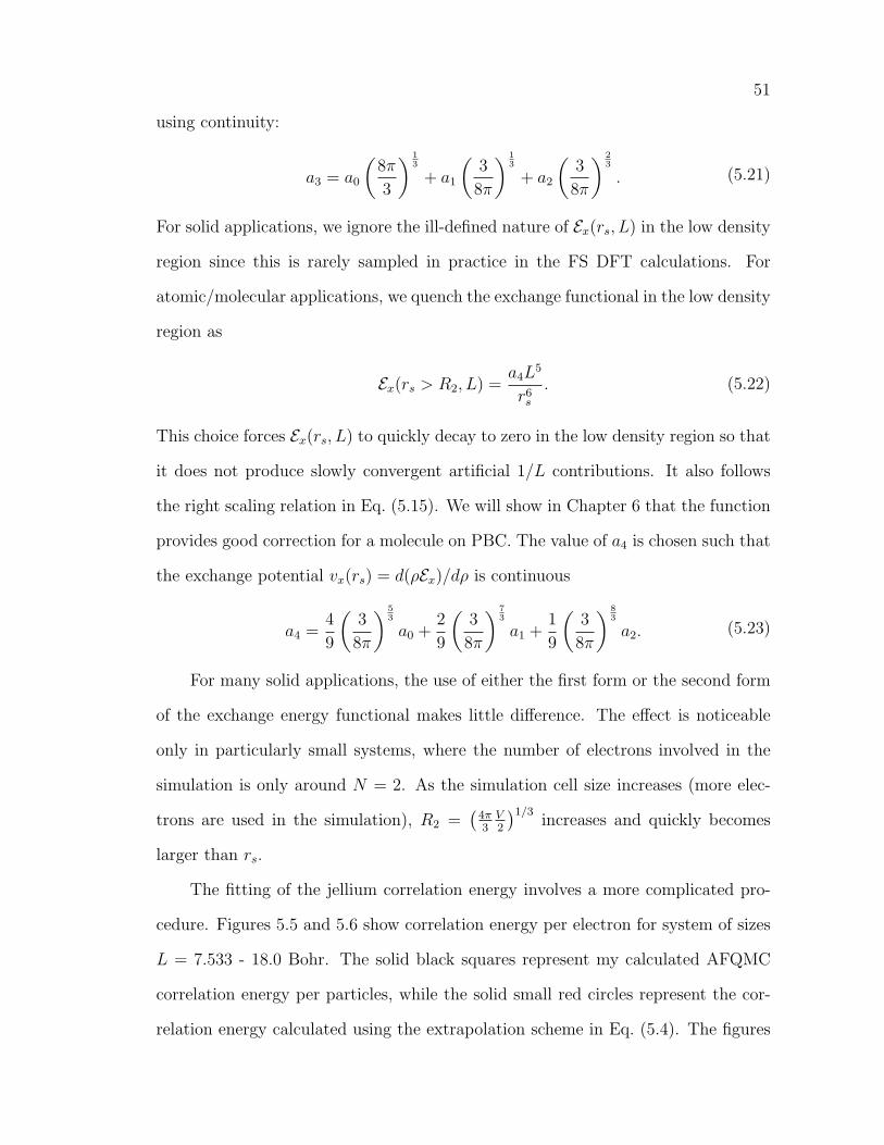
51
using continuity:
a3 = a0
(8π
3
) 13
+ a1
(3
8π
) 13
+ a2
(3
8π
) 23
. (5.21)
For solid applications, we ignore the ill-defined nature of Ex(rs, L) in the low density
region since this is rarely sampled in practice in the FS DFT calculations. For
atomic/molecular applications, we quench the exchange functional in the low density
region as
Ex(rs > R2, L) =a4L
5
r6s
. (5.22)
This choice forces Ex(rs, L) to quickly decay to zero in the low density region so that
it does not produce slowly convergent artificial 1/L contributions. It also follows
the right scaling relation in Eq. (5.15). We will show in Chapter 6 that the function
provides good correction for a molecule on PBC. The value of a4 is chosen such that
the exchange potential vx(rs) = d(ρEx)/dρ is continuous
a4 =4
9
(3
8π
) 53
a0 +2
9
(3
8π
) 73
a1 +1
9
(3
8π
) 83
a2. (5.23)
For many solid applications, the use of either the first form or the second form
of the exchange energy functional makes little difference. The effect is noticeable
only in particularly small systems, where the number of electrons involved in the
simulation is only around N = 2. As the simulation cell size increases (more elec-
trons are used in the simulation), R2 =(
4π3V2
)1/3increases and quickly becomes
larger than rs.
The fitting of the jellium correlation energy involves a more complicated pro-
cedure. Figures 5.5 and 5.6 show correlation energy per electron for system of sizes
L = 7.533 - 18.0 Bohr. The solid black squares represent my calculated AFQMC
correlation energy per particles, while the solid small red circles represent the cor-
relation energy calculated using the extrapolation scheme in Eq. (5.4). The figures

52
show that the extrapolation scheme works well for the high density region (large
number of electrons), but is not accurate in the low density region (small number
of electrons). These results are not surprising, since the asymptotic expression in
Eq. (5.4) is obtained from QMC simulations with large number of electrons. The
more accurate fit (solid line) is described below.
We express the correlation energy per particle in the following form
Ec(L, rs) =
E∞c (rs)−
a1
L2rs +
g(rs)
L3rs < Rh
h(rs) Rh < rs < Rl
0 Rl < rs
, (5.24)
where the E∞c (rs) is the correlation energy per particle for infinite-size jellium at
density rs [Eq. (5.9)], and the −a1rs/L2 factor exactly cancels the corresponding
term in Ex(rs, L) [Eq. (5.19)], since Exc(rs, L) should converge as 1/L3. Note that
there is no L dependence in g(rs), which makes this function universal for all (cubic)
simulation cell sizes. Rh and Rl are defined below.
The function g(rs) is fitted (to Eq. 5.4 for rs < Rh) to the following form
g(rs) = d1 ln rs + d2rs + d3r32s + d4r
2s . (5.25)
The g(rs) plot is given in Fig. 5.7. As indicated in the figure, the values of g(rs)
obtained from extrapolation are good only for large numbers of particle (small rs).
For small number of particles (N . 12), the QMC calculated energies are higher
than the energies calculated with the extrapolation.
For the low density region, rs ≥ Rl where Rl = rs(N = 0.5), the correlation is
set to be zero. In the intermediate density region, Rh ≤ rs ≤ Rl where Rh ≡ rs(N =
12) = L ·(
348π
)1/3, the correlation energy per particle is given as a polynomial h(rs)
h(rs) = e1 + e2rs + e3r2s + e4r
3s . (5.26)
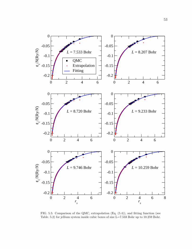
53
0 2 4 6
-0.2
-0.15
-0.1
-0.05
0ε c/N
(Ry/
N)
QMCExtrapolationFitting
0 2 4 6
-0.2
-0.15
-0.1
-0.05
0
0 2 4 6
-0.2
-0.15
-0.1
-0.05
0
ε c/N(R
y/N
)
0 2 4 6
-0.2
-0.15
-0.1
-0.05
0
0 2 4 6r
s
-0.2
-0.15
-0.1
-0.05
0
ε c/N(R
y/N
)
0 2 4 6 8r
s
-0.2
-0.15
-0.1
-0.05
0
L = 7.533 Bohr L = 8.207 Bohr
L = 8.720 Bohr L = 9.233 Bohr
L = 9.746 Bohr L = 10.259 Bohr
FIG. 5.5: Comparison of the QMC, extrapolation (Eq. (5.4)), and fitting function (seeTable. 5.2) for jellium system inside cubic boxes of size L=7.533 Bohr up to 10.259 Bohr.
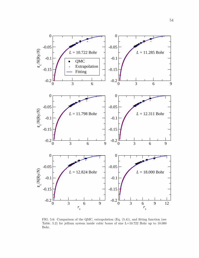
54
0 3 6-0.2
-0.15
-0.1
-0.05
0ε c/N
(Ry/
N)
QMCExtrapolationFitting
0 3 6 9-0.2
-0.15
-0.1
-0.05
0
0 3 6 9-0.2
-0.15
-0.1
-0.05
0
ε c/N(R
y/N
)
0 3 6 9-0.2
-0.15
-0.1
-0.05
0
0 3 6 9r
s
-0.2
-0.15
-0.1
-0.05
0
ε c/N(R
y/N
)
0 3 6 9 12r
s
-0.2
-0.15
-0.1
-0.05
0
L = 10.722 Bohr L = 11.285 Bohr
L = 11.798 Bohr L = 12.311 Bohr
L = 12.824 Bohr L = 18.000 Bohr
FIG. 5.6: Comparison of the QMC, extrapolation (Eq. (5.4)), and fitting function (seeTable. 5.2) for jellium system inside cubic boxes of size L=10.722 Bohr up to 18.000Bohr.

55
0 1 2 3 4 5 6 7r
s
-120
-100
-80
-60
-40
-20
0
g(r s)
ExtrapolationQMC L = 7.533 BohrQMC L = 10.259 BohrQMC L = 12.824 Bohr
FIG. 5.7: Comparison of g(rs) obtained from extrapolation and QMC calculations. Theextrapolation values are only accurate for large number of particles, as indicated by goodagreement between QMC values and extrapolation values. For small number of particles,QMC values of g(rs) differ from the extrapolation curve, which break down.
The parameter e1, e2, e3 and e4 are completely determined from continuity condi-
tions at Rl and Rh,
ei =e1i
LiEc(Rh, L) +
e2i
Li−1
dEc(rs, L)
drs
∣∣∣∣rs=Rh
, (5.27)
where Ec(Rh, L) and dEc(rs,L)drs
|rs=Rh are the value and the first derivative of correlation
energy per particle in the high density region.
Detail of the FS exchange correlation functions are summarized in Table 5.2
and the parameter values are presented in Table 5.3. Figures 5.5 and 5.6 show that
the fitting function (solid line) well describes both the high and low density regions.
It matches both the present AFQMC results as well as the extrapolation results
[eq. (5.4)] in the high density region. The calculations shown in Figures 5.5 and 5.6
cover a range of supercell sizes from (7.5 Bohr)3 to (18 Bohr)3.
The final FS exchange and correlation energy per particle are shown for several

56
TABLE 5.2: Summary of the FS exchange and correlation functions
function form region
Ex(rs, L)
a0
rs+a1rsL2
+a2r
2s
L3rs ≤ R2
f(rs, L) R2 < rs
f(rs, L)
a3
Lfor solid systems
a4L5
r6s
for atomic/molecularsystem
R2(L) L ·(
3
8π
) 13
E∞x (rs)a0
rsall region
Ec(rs, L)E∞c (rs)−
a1rsL2
+g(rs)
L3rs ≤ Rh
h(rs, L) Rh < rs ≤ Rl
0 Rl < rs
g(rs) d1rs ln rs + d2rs + d3r32s + d4r
2s
h(rs) e1 + e2rs + e3r2s + e4r
3s
eie1i
LiEc(Rh, L) +
e2i
Li−1
dEc(rs, L)
drs
∣∣∣∣rs=Rh
Rh(L) L ·(
3
48π
) 13
Rl(L) L ·(
3
4π
) 13
E∞c (rs)c1 ln rs + c2 + c3rs ln rs + c4rs rs ≤ 1
c5
1 + c6√rs + c7rs
1 < rs

57
TABLE 5.3: Numerical values of parameters used in Table. 5.2. All parameters are givenin Rydberg atomic unit.
parameter value parameter valuea0 -0.9163 d1 0.1182a1 -2.2037 d2 1.1656a2 0.4710 d3 -5.2884a3 -2.8373 d4 -1.1233a4 -0.0150 e11 -0.1436c1 0.0622 e12 9.5439c2 -0.096 e13 -23.7164c3 0.0040 e14 15.0215c4 -0.0232 e21 -0.6348c5 -0.2846 e22 3.9673c6 1.0529 e23 -7.0343c7 0.3334 e24 3.8352
simulation cell sizes in Fig. 5.8. The FS exchange energies approach the infinite-
size limit from below, while the FS correlation energies approach it from above.
This is the reason why the HF method gives too large a correction, since it does not
include the correlation energy. In the exchange functional (top panel of Fig. 5.8) the
dashed line represents the choice of the low density (rs > R2) for atomic/molecular
systems with PBC [Eq. (5.22)] and the dot-dashed line represents the low density
choice [Eq. (5.20)] for solids. As the simulation cell size increases, R2 [visualized by
the discontinuity in Fig. 5.8] moves to lower densities, where it makes smaller and
smaller contributions.
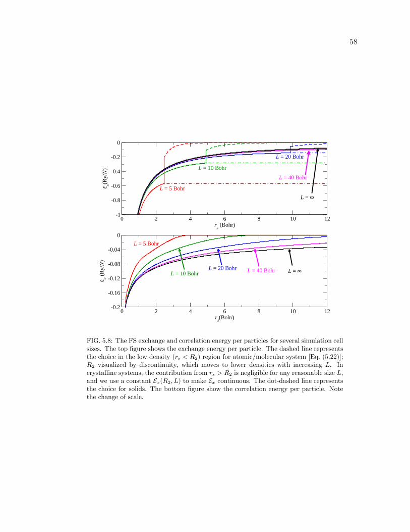
58
0 2 4 6 8 10 12r
s (Bohr)
-1
-0.8
-0.6
-0.4
-0.2
0
ε x(Ry/
N)
0 2 4 6 8 10 12r
s(Bohr)
-0.2
-0.16
-0.12
-0.08
-0.04
0
ε c (R
y/N
)
L = 5 Bohr
L = 10 Bohr
L = 20 Bohr
L = 40 Bohr
L = ∞
L = 5 Bohr
L = 10 BohrL = 20 Bohr L = 40 Bohr L = ∞
FIG. 5.8: The FS exchange and correlation energy per particles for several simulation cellsizes. The top figure shows the exchange energy per particle. The dashed line representsthe choice in the low density (rs < R2) region for atomic/molecular system [Eq. (5.22)];R2 visualized by discontinuity, which moves to lower densities with increasing L. Incrystalline systems, the contribution from rs > R2 is negligible for any reasonable size L,and we use a constant Ex(R2, L) to make Ex continuous. The dot-dashed line representsthe choice for solids. The bottom figure show the correlation energy per particle. Notethe change of scale.

CHAPTER 6
Applications of Finite Size
Correction
In this chapter, applications of the new size-correction method are presented
on several types of systems. After discussing some technical details on how to use
the FS XC function, I will report applications on the P2 molecule, bulk fcc silicon,
metallic bulk bcc sodium, and perovskite structure BiScO3.
6.1 Correction Scheme
The infinite-size limit of a many-body calculation is obtained from the FS many-
body calculations after applying one-body and two-body FS corrections,
E∞ = E(Ω) + ∆E1−b(Ω) + ∆E2−b(Ω), (6.1)
where Ω is the volume of the simulation cell. The FS dependence on the simulation
cell size and shape is shown as a function of Ω only, where Ω = L3, which is
approximate except for cubic cells. We will return to this later in this chapter. The
approach in Eq. (6.1) is valid if the one-body FS error is well separated from the
59
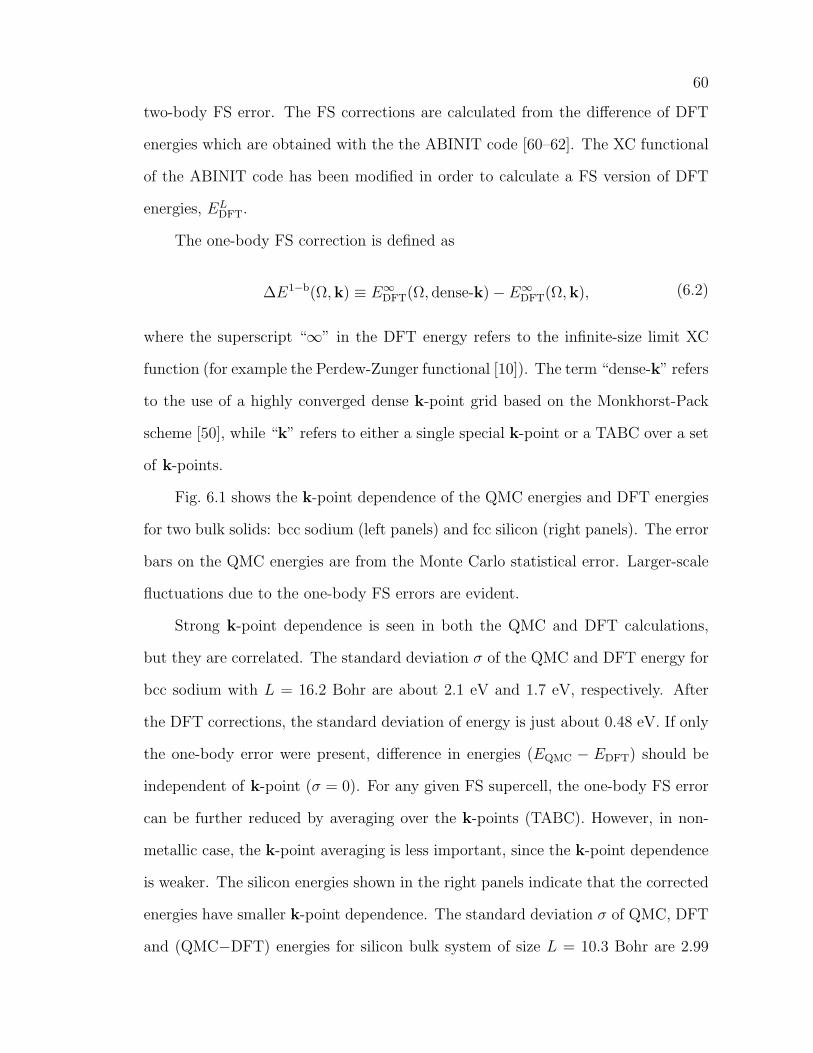
60
two-body FS error. The FS corrections are calculated from the difference of DFT
energies which are obtained with the the ABINIT code [60–62]. The XC functional
of the ABINIT code has been modified in order to calculate a FS version of DFT
energies, ELDFT.
The one-body FS correction is defined as
∆E1−b(Ω,k) ≡ E∞DFT(Ω, dense-k)− E∞DFT(Ω,k), (6.2)
where the superscript “∞” in the DFT energy refers to the infinite-size limit XC
function (for example the Perdew-Zunger functional [10]). The term “dense-k” refers
to the use of a highly converged dense k-point grid based on the Monkhorst-Pack
scheme [50], while “k” refers to either a single special k-point or a TABC over a set
of k-points.
Fig. 6.1 shows the k-point dependence of the QMC energies and DFT energies
for two bulk solids: bcc sodium (left panels) and fcc silicon (right panels). The error
bars on the QMC energies are from the Monte Carlo statistical error. Larger-scale
fluctuations due to the one-body FS errors are evident.
Strong k-point dependence is seen in both the QMC and DFT calculations,
but they are correlated. The standard deviation σ of the QMC and DFT energy for
bcc sodium with L = 16.2 Bohr are about 2.1 eV and 1.7 eV, respectively. After
the DFT corrections, the standard deviation of energy is just about 0.48 eV. If only
the one-body error were present, difference in energies (EQMC − EDFT) should be
independent of k-point (σ = 0). For any given FS supercell, the one-body FS error
can be further reduced by averaging over the k-points (TABC). However, in non-
metallic case, the k-point averaging is less important, since the k-point dependence
is weaker. The silicon energies shown in the right panels indicate that the corrected
energies have smaller k-point dependence. The standard deviation σ of QMC, DFT
and (QMC−DFT) energies for silicon bulk system of size L = 10.3 Bohr are 2.99
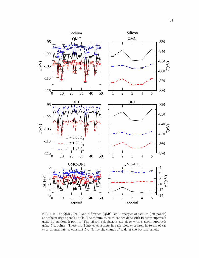
61
0 10 20 30 40 50-115
-110
-105
-100
-95
E(e
V)
0 10 20 30 40 50-115
-110
-105
-100
-95E
(eV
)
L = 0.80 L0
L = 1.00 L0
L = 1.25 L0
0 10 20 30 40 50k-point
-5
-4
-3
-2
-1
0
∆E (
eV)
1 2 3 4 5-880
-870
-860
-850
-840
-830
E(e
V)
1 2 3 4 5-870
-860
-850
-840
-830
-820
E(e
V)
1 2 3 4 5k-point
-14
-12
-10
-8
-6
-4∆E
(eV
)
QMC
DFT
QMC-DFT
QMC
DFT
QMC-DFT
Sodium Silicon
FIG. 6.1: The QMC, DFT and difference (QMC-DFT) energies of sodium (left panels)and silicon (right panels) bulk. The sodium calculations are done with 16 atom supercellsusing 50 random k-points. The silicon calculations are done with 8 atom supercellsusing 5 k-points. There are 3 lattice constants in each plot, expressed in terms of theexperimental lattice constant L0. Notice the change of scale in the bottom panels.
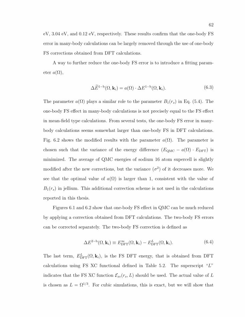
62
eV, 3.04 eV, and 0.12 eV, respectively. These results confirm that the one-body FS
error in many-body calculations can be largely removed through the use of one-body
FS corrections obtained from DFT calculations.
A way to further reduce the one-body FS error is to introduce a fitting param-
eter a(Ω),
∆E1−b(Ω,ki) = a(Ω) ·∆E1−b(Ω,ki). (6.3)
The parameter a(Ω) plays a similar role to the parameter B1(rs) in Eq. (5.4). The
one-body FS effect in many-body calculations is not precisely equal to the FS effect
in mean-field type calculations. From several tests, the one-body FS error in many-
body calculations seems somewhat larger than one-body FS in DFT calculations.
Fig. 6.2 shows the modified results with the parameter a(Ω). The parameter is
chosen such that the variance of the energy difference (EQMC − a(Ω) · EDFT) is
minimized. The average of QMC energies of sodium 16 atom supercell is slightly
modified after the new corrections, but the variance (σ2) of it decreases more. We
see that the optimal value of a(Ω) is larger than 1, consistent with the value of
B1(rs) in jellium. This additional correction scheme is not used in the calculations
reported in this thesis.
Figures 6.1 and 6.2 show that one-body FS effect in QMC can be much reduced
by applying a correction obtained from DFT calculations. The two-body FS errors
can be corrected separately. The two-body FS correction is defined as
∆E2−b(Ω,ki) ≡ E∞DFT(Ω,ki)− ELDFT(Ω,ki). (6.4)
The last term, ELDFT(Ω,ki), is the FS DFT energy, that is obtained from DFT
calculations using FS XC functional defined in Table 5.2. The superscript “L”
indicates that the FS XC function Exc(rs, L) should be used. The actual value of L
is chosen as L = Ω1/3. For cubic simulations, this is exact, but we will show that
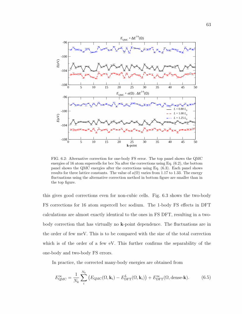
63
0 5 10 15 20 25 30 35 40 45 50-108
-104
-100
-96
E(e
V)
0 5 10 15 20 25 30 35 40 45 50k-point
-108
-104
-100
-96
E(e
V)
L = 0.80 L0
L = 1.00 L0
L = 1.25 L0
EQMC
+ ∆E1-b
(Ω)
EQMC
+ a(Ω) . ∆E1-b
(Ω)
FIG. 6.2: Alternative correction for one-body FS error. The top panel shows the QMCenergies of 16 atom supercells for bcc Na after the corrections using Eq. (6.2), the bottompanel shows the QMC energies after the corrections using Eq. (6.3). Each panel showsresults for three lattice constants. The value of a(Ω) varies from 1.17 to 1.33. The energyfluctuations using the alternative correction method in bottom figure are smaller than inthe top figure.
this gives good corrections even for non-cubic cells. Fig. 6.3 shows the two-body
FS corrections for 16 atom supercell bcc sodium. The 1-body FS effects in DFT
calculations are almost exactly identical to the ones in FS DFT, resulting in a two-
body correction that has virtually no k-point dependence. The fluctuations are in
the order of few meV. This is to be compared with the size of the total correction
which is of the order of a few eV. This further confirms the separability of the
one-body and two-body FS errors.
In practice, the corrected many-body energies are obtained from
E∞QMC =1
Nk
Nk∑i
(EQMC(Ω,ki)− EL
DFT(Ω,ki))
+ E∞DFT(Ω, dense-k). (6.5)

64
-110
-105
-100
-95
E(e
V)
L = 0.80 L0
L = 1.00 L0
L = 1.25 L0
-110
-105
-100
-95
E(e
V)
0 5 10 15 20 25 30 35 40 45 50k-point
1
2
3
4
∆E(e
V)
DFT
FS DFT
2-body correction = DFT - FS DFT
FIG. 6.3: The energies of DFT (top panel) and FS DFT (middle panel) calculated for50 random k-points. The 3 curves in each panel are the energies for 3 lattice constants.The bottom panel shows the two-body FS correction, as defined in Eq. (6.4).
This twist averaging over k-point is efficient for stochastic method like QMC, since
the averaging also helps reduce the statistical noise [52]. As shown before, while the
fluctuations of EQMC(Ω,ki) and EDFT(Ω,ki) are individually large, the difference
has a smaller variance. It is therefore better to average over the difference to reduce
statistical error. The last term E∞DFT(V, dense-k) is k-point independent, and can
therefore be obtained from any supercell. To reduce the computational cost, we
simply use the primitive cell to obtain this term. Eq. (6.5) can be rewritten by
adding and subtracting a E∞DFT(Ω,ki),
E∞QMC =1
Nk
Nk∑i
(EQMC(Ω,ki)− E∞DFT(Ω,ki))
+1
Nk
Nk∑i
(E∞DFT(Ω,ki)− EL
DFT(Ω,ki))
+ E∞DFT(Ω, dense-k).
(6.6)
65
If the second term in Eq. (6.6) is neglected, this is just the one-body corrected
QMC energy (with TBC). The major advantage of the one-body FS correction is
that it reduces energy fluctuations due to k-point sampling, while the two-body FS
correction improves physical properties of the system, such as the equilibrium lattice
constant and the bulk modulus.
Since two-body FS correction was shown to have little k-point dependence, it
can be obtained by using sampling over only a few k-points or by just using a single
calculation with a dense k-point grid,
∆E2−b(Ω) = E∞DFT(Ω, dense-k)− ELDFT(Ω, dense-k). (6.7)
As before, this quantity can be calculated using the primitive cell with the proper
XC function. In this case, the notation is as follows: the superscript L refers to
the size of the supercell whose FS Exc(rs, L) is used, while Ω is the volume of the
primitive cell.
6.2 P2 Molecule
The first application presented here is for the ground state energy of the P2
molecule, using supercells and periodic boundary condition. The FS effect of this
system is illustrated in plot a. of Fig. 5.1. Here the FS correction is defined as
E∞QMC = EQMC(Ω,Γ) +[E∞DFT(Ω→∞,Γ)− EL
DFT(Ω,Γ)], (6.8)
since all calculations were done using only the Γ-point (k = 0). This choice is reason-
able for an atom or a molecule inside a large supercell calculation. The infinite-size
limit of DFT energy E∞DFT(Ω → ∞,Γ) is obtained by direct extrapolation using
very large simulation cells and the specific boundary condition (k-points) has little
effect.

66
8 10 12 14 16 18 20L (Bohr)
-370
-368
-366
-364
-362
-360
-358
-356
Ene
rgy
(eV
)
QMCDFT
∞
DFTFS
QMC + ∆DFT∞
QMC + ∆DFTFS
0 0.001 0.002 0.003
1/Ω
-364
-362
-360
FIG. 6.4: The QMC energy of the P2 molecule using supercells and periodic boundarycondition. The dashed and dotted lines are the DFT energies calculated with the infinite-size XC function and the FS XC function, respectively. The blue solid line with circles isthe QMC energy. The the dashed line with boxes and the dotted lines with diamonds arethe QMC energy after correction with the infinite-size limit and FS DFT XC function,respectively. The inset shows the same energy plotted with respect to 1/Ω.
The core states of the P atom are represented with a norm conserving pseu-
dopotential generated using OPIUM [30]. Calculations of the P2 molecule at experi-
mental equilibrium bondlength of 3.578 Bohr were performed for cubic supercells of
size (7 Bohr)3 to (18 Bohr)3 using auxiliary field quantum Monte Carlo (AFQMC)
[17]. Fig. 6.4 shows the energies calculated with QMC, DFT∞ and DFTFS. The
superscript “∞” in DFT∞ indicated that the infinite-size limit XC function is used.
DFT∞ yields the conventional correction
∆DFT∞ = E∞DFT(Ω→∞,Γ)− E∞DFT(Ω,Γ), (6.9)

67
while DFTFS is used to calculate the new FS XC correction
∆DFTFS = E∞DFT(Ω→∞,Γ)− ELDFT(Ω,Γ). (6.10)
As seen in Fig. 6.4, the conventional DFT∞ energy converges very rapidly to
the infinite limit. The energy at (18 Bohr)3 differs from its infinite-size limit by less
then 4 meV. By contrast the QMC error is 310 meV, and the slow convergence of
the DFT-corrected-QMC energy (QMC + ∆DFT∞) is evident. DFTFS, however,
shows similar size convergence to QMC, yielding a better correction scheme. With
these corrections, the corrected energy has an error of about 34±91 meV at the size
of (18 Bohr)3. The inset in Fig. 6.4 shows that the QMC energy corrected with the
new scheme gives not only a more linear-curve as a function of 1/Ω, but also has a
smaller slope. Accurate extrapolation to infinite-size is thus possible.
6.3 Fcc Silicon
Fcc silicon has the diamond structure with 2 atoms per primitive unit cell, lo-
cated at the origin and at (14
14
14) in reduced coordinates. Here I apply the new FS
correction on previously published DMC results [47] and show that the new cor-
rection accelerates the size convergence [3]. The pseudopotential used is different
from that in the DMC calculations. We used multiple pseudopotentials to ensure
that the FS correction are independent of the choice of pseudopotential. The DMC
calculations were for n × n × n supercells of the primitive (non-cubic) cell. Never-
theless, the new correction significantly improves the convergence, indicating that
the correction also works with non-cubic simulation cells. Finally, I will present re-
sults for the equilibrium lattice constant, bulk modulus and cohesive energy. These
properties are calculated for supercells with number of atom equal to 8 and 16 using
AFQMC.
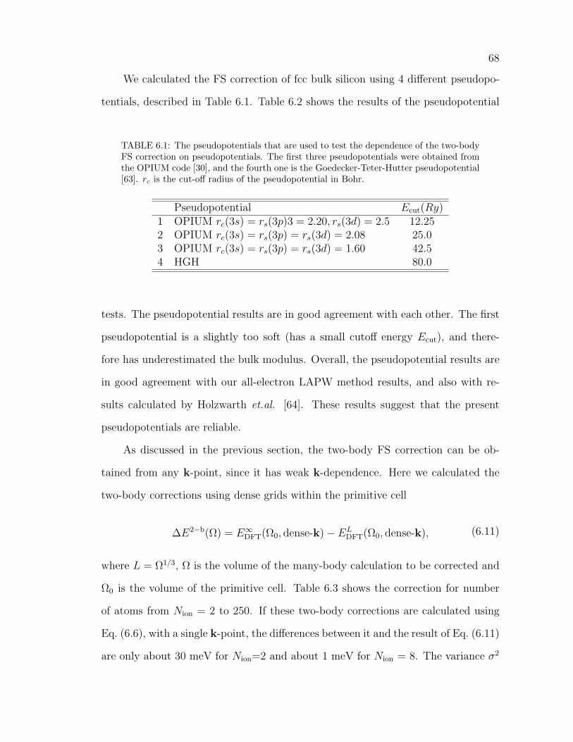
68
We calculated the FS correction of fcc bulk silicon using 4 different pseudopo-
tentials, described in Table 6.1. Table 6.2 shows the results of the pseudopotential
TABLE 6.1: The pseudopotentials that are used to test the dependence of the two-bodyFS correction on pseudopotentials. The first three pseudopotentials were obtained fromthe OPIUM code [30], and the fourth one is the Goedecker-Teter-Hutter pseudopotential[63]. rc is the cut-off radius of the pseudopotential in Bohr.
Pseudopotential Ecut(Ry)1 OPIUM rc(3s) = rs(3p)3 = 2.20, rs(3d) = 2.5 12.252 OPIUM rc(3s) = rs(3p) = rs(3d) = 2.08 25.03 OPIUM rc(3s) = rs(3p) = rs(3d) = 1.60 42.54 HGH 80.0
tests. The pseudopotential results are in good agreement with each other. The first
pseudopotential is a slightly too soft (has a small cutoff energy Ecut), and there-
fore has underestimated the bulk modulus. Overall, the pseudopotential results are
in good agreement with our all-electron LAPW method results, and also with re-
sults calculated by Holzwarth et.al. [64]. These results suggest that the present
pseudopotentials are reliable.
As discussed in the previous section, the two-body FS correction can be ob-
tained from any k-point, since it has weak k-dependence. Here we calculated the
two-body corrections using dense grids within the primitive cell
∆E2−b(Ω) = E∞DFT(Ω0, dense-k)− ELDFT(Ω0, dense-k), (6.11)
where L = Ω1/3, Ω is the volume of the many-body calculation to be corrected and
Ω0 is the volume of the primitive cell. Table 6.3 shows the correction for number
of atoms from Nion = 2 to 250. If these two-body corrections are calculated using
Eq. (6.6), with a single k-point, the differences between it and the result of Eq. (6.11)
are only about 30 meV for Nion=2 and about 1 meV for Nion = 8. The variance σ2

69
TABLE 6.2: Several physical properties calculated with the four pseudopotentials inTable. 6.1. The results are compared with our own all electron LAPW results and withthe pseudopotential and LAPW calculations from Ref. [64].
Lattice Bulk Cohesiveconstant (Bohr) modulus (GPa) energy (eV)[a]
This workPseudopotential 1 10.175 93 5.33Pseudopotential 2 10.180 95 5.33Pseudopotential 3 10.170 97 5.36Pseudopotential 4 10.171 96 5.33LAPW 10.214 97 5.19
Ref. [64]Pseudopotential 10.186 98 –LAPW 10.223 98 –
experiment [65] 10.261 99 4.63
[a] Cohesive energies from Ref. [64] are not shown, since they used a non-spin-polarized Si atom
due to the different pseudopotential is very small. We also note that the two-body
correction is essentially linear versus 1/Nion (see the inset in Fig. 6.5 below).
The raw DMC energies were calculated by Kent et al. [47] for system sizes of
n = 1, 2, 3, 4, and 5, corresponding to Nion = 2, 16, 54, 128, and 250 atoms. These
calculations only used single k-point, (the L-point). Fig. 6.5 shows the raw DMC
energies, together with the energies after one-body and two-body corrections. Also
shown are results using a modified periodic Coulomb (MPC) interaction [47] (see
also discussion in section 5.2 ). The one-body correction ∆E1−b has an opposite
direction (approaching infinite-size limit from above) and therefore increases the FS
error. For the smallest system, it increases the error by more than 50%, but for
larger systems (n=3) the one body correction is essentially zero (less than 10 meV).
The MPC improves the energies by about 0.44 eV for smallest simulation cell n = 1,
while for n = 3, the improvement is only 11 meV. The new FS correction improves

70
TABLE 6.3: The two-body correction for 4 pseudopotentials (in eV). Na is the numberof atoms. The parameter L indicates the effective volume of the cell L = Ω1/3 (in Bohr).Results are shown for fcc and cubic supercells.
L pseudopotentialN (Bohr) supercell 1 2 3 42 6.4638494 fcc 2.7429 2.7357 2.7381 2.73438 10.2607213 cubic 0.7117 0.7101 0.7106 0.709816 12.9276988 fcc 0.3568 0.3560 0.3563 0.355954 19.3915481 fcc 0.1057 0.1055 0.1056 0.105464 20.5214426 cubic 0.0892 0.0890 0.0891 0.0890128 25.8553975 fcc 0.0446 0.0445 0.0445 0.0445216 30.7821639 cubic 0.0264 0.0264 0.0264 0.0264250 32.3192469 fcc 0.0228 0.0228 0.0228 0.0228
1 2 3 4 5system size (n)
-3
-2
-1
0
∆E/a
tom
(eV
)
raw DMC
DMC + ∆E1-b
MPC
DMC + ∆E1-b
+ ∆E2-b
0 0.1 0.2 0.3 0.4 0.51/N
a
0
0.5
1
1.5
2
2.5
3
∆E2-
b (eV
)
FIG. 6.5: Total energy per atom of silicon as a function of simulation cell size n. Thevertical axis is defined as ∆E ≡ E(Na)−E∞. The black circles represent the raw energies(DMC), the one-body corrected energies are given by red squares. The fully correctedenergies are shown by blue triangles. MPC energies, calculated by Kent et al. [47], areshown as the green diamonds. The inset show the volume dependence of two-body FSerror. Both cubic and fcc results lie on the same linear curve.

71
the energy about 1.45 eV for the smallest cell n = 1, and still give a correction of
96 meV for system size of n = 3. The overall size corrections are systematically
improved.
Next we calculate the equilibrium lattice constant, bulk modulus and cohesive
energy of silicon. The AFQMC method was used for the rest of fcc silicon appli-
cations. The pseudopotential used here is the second pseudopotential in Table 6.1
with Ecut of 25 Ry. The silicon atomic energy is needed to calculate the cohesive
energy of the crystal. Fig. 6.6 shows results of atomic calculations inside supercell of
sizes (14 Bohr)3 to (20 Bohr)3 with PBC. The infinite-size limit is obtained through
the extrapolation. The FS correction can not yet be applied here, because it was
designed for non-spin-polarized systems. A linear fit yields an extrapolated atomic
energy of −103.33± 0.02 eV.
0 1 2 3 4
1/Ω (unit of 10-4
a0
-3)
-103.7
-103.6
-103.5
-103.4
-103.3
Ene
rgy
(eV
)
E = -103.33 -875.46/Ω
(20)3
(19)3
(18)3
(17)3
(16)3
(15)3
(14)3
FIG. 6.6: The silicon atom total energy for simulation cell of sizes (14 Bohr)3 to (20Bohr)3. The FS correction can not be applied to this atom because silicon atom hasa spin polarization due to two spin up electrons at orbital 2p. The infinite-size limit isobtained through extrapolation.

72
Convergence of the total energy is shown in Fig. 6.7. The total energy of
silicon bulk has already well converged at Ecut = 25 Ry for both DFT and QMC
calculations.
10 20 30 40 50E
cut (Ry)
-870
-860
-850
-840
-830
-820
Ene
rgy
(eV
)
L = 0.80 L0
L = L0
L = 1.25 L0
20 25 30 35 40 45E
cut (Ry)
-880
-870
-860
-850
-840
-830
Ene
rgy
(eV
)
FIG. 6.7: Convergence of the total energy of an 8 atom Si supercell for 3 lattice constants,calculated using DFT (left panel) and QMC (right panel). At Ecut = 25 Ry, the energyhas already reached convergence.
The Trotter error, which arises from neglecting higher order terms when the
imaginary time propagator e−∆τH is decomposed into one-body and two-body oper-
ators in Eq. (3.39), is shown in Fig. 6.8. The total energy of an 8 atom Si supercell
calculated with ∆τ = 0.04 (in Rydberg atomic unit) is in good agreement with the
energy calculated with ∆τ = 0.01. This result suggests that the Trotter error of
calculations using ∆τ = 0.01 is already smaller than statistical errors.
Table 6.4 shows the equilibrium lattice constant, bulk modulus and cohesive
energy of the Si. The QMC energy shown in Fig. 6.9 were fit to Murnaghan’s

73
0 0.01 0.02 0.03 0.04 0.05∆τ
-64.5
-64
-63.5
-63
-62.5
-62
Ene
rgy
(Ry)
L = 0.80 L0
L = L0
L = 1.25L0
FIG. 6.8: Trotter error for 8 atom supercell of silicon bulk for 3 lattice constants. Rydbergatomic unit is used in this figure. The production calculations are done using ∆τ = 0.01.
equations [66] to obtain these physical properties,
E = E0 +3
2Ω0B0
[3
4(1 + 2δ)
(Ω0
Ω
)4/3
− δ
2
(Ω0
Ω
)2
−3
2(1 + δ)
(Ω0
Ω
)2/3
+1
2
(δ +
3
2
)],
(6.12)
where Ω0 is the equilibrium volume, B0 is the zero-pressure bulk modulus, δ =
(3 − 3B′0/4) and B′0 is the derivative of bulk modulus with respect to pressure at
zero pressure. In the applications, we simply fit the data to equivalent equation
E = E0 +E1
Ω2/3+
E2
Ω4/3+E3
Ω2, (6.13)
and the equilibrium lattice constant is determined by the lattice constant that min-
imize the energy (indicated by black arrows in Fig. 6.9) and the bulk modulus is
determined by B = Ω · ∂2E∂Ω2 at equilibrium lattice constant. Cohesive energy is the
energy per atom needed to decompose the solid into atoms (indicated as the dashed
arrows in Fig. 6.9).
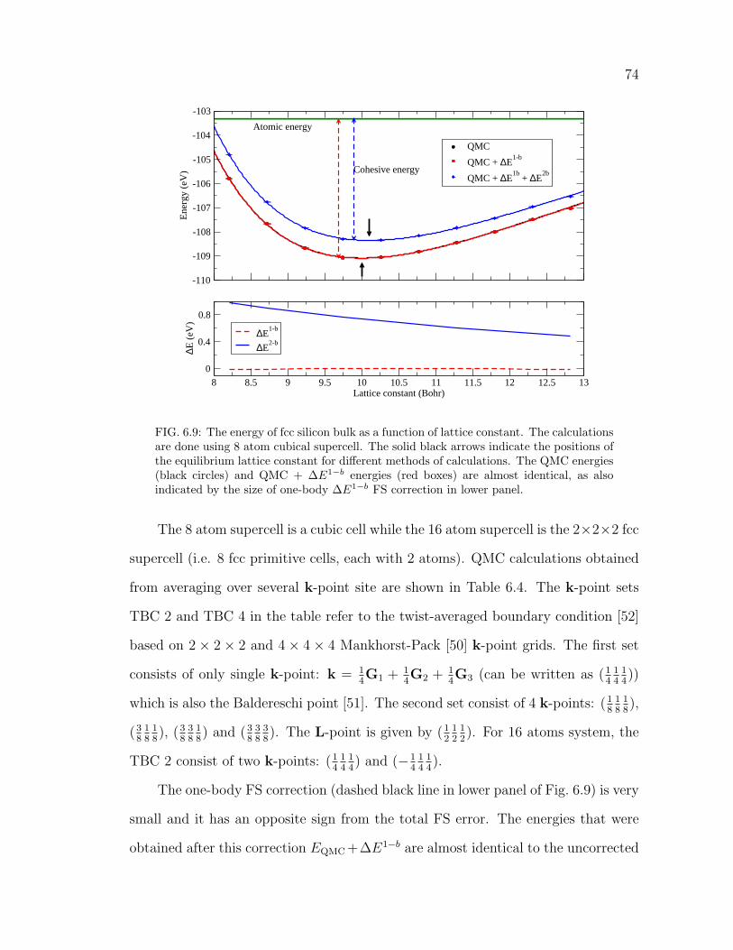
74
-110
-109
-108
-107
-106
-105
-104
-103
Ene
rgy
(eV
)
QMC
QMC + ∆E1-b
QMC + ∆E1b
+ ∆E2b
8 8.5 9 9.5 10 10.5 11 11.5 12 12.5 13Lattice constant (Bohr)
0
0.4
0.8
∆E (
eV)
∆E1-b
∆E2-b
Atomic energy
Cohesive energy
FIG. 6.9: The energy of fcc silicon bulk as a function of lattice constant. The calculationsare done using 8 atom cubical supercell. The solid black arrows indicate the positions ofthe equilibrium lattice constant for different methods of calculations. The QMC energies(black circles) and QMC + ∆E1−b energies (red boxes) are almost identical, as alsoindicated by the size of one-body ∆E1−b FS correction in lower panel.
The 8 atom supercell is a cubic cell while the 16 atom supercell is the 2×2×2 fcc
supercell (i.e. 8 fcc primitive cells, each with 2 atoms). QMC calculations obtained
from averaging over several k-point site are shown in Table 6.4. The k-point sets
TBC 2 and TBC 4 in the table refer to the twist-averaged boundary condition [52]
based on 2 × 2 × 2 and 4 × 4 × 4 Mankhorst-Pack [50] k-point grids. The first set
consists of only single k-point: k = 14G1 + 1
4G2 + 1
4G3 (can be written as (1
414
14))
which is also the Baldereschi point [51]. The second set consist of 4 k-points: (18
18
18),
(38
18
18), (3
838
18) and (3
838
38). The L-point is given by (1
212
12). For 16 atoms system, the
TBC 2 consist of two k-points: (14
14
14) and (−1
414
14).
The one-body FS correction (dashed black line in lower panel of Fig. 6.9) is very
small and it has an opposite sign from the total FS error. The energies that were
obtained after this correction EQMC +∆E1−b are almost identical to the uncorrected

75
TABLE 6.4: The equilibrium lattice constant, bulk modulus and cohesive energy ofsilicon bulk. Na is the number of atoms used in calculations. TBC 2 and TBC 4 aretwist-averaged boundary condition [52] based on 2× 2× 2 and 4× 4× 4 Mankhorst-Pack[50] k-point grids, respectively. ∆E = ∆E1−b + ∆E2−b. The cohesive energies containa correction for the zero-point energy of the solid of EZPE=0.06 eV per atom.
N k-point lattice bulk cohesiveconstant (Bohr) modulus (GPa) energy (eV)
QMC 8 TBC 2 10.01± 0.03 112± 4 5.59± 0.06QMC 8 TBC 4 9.96± 0.02 103± 4 5.66± 0.04
QMC + ∆E1−b 8 TBC 2 10.00± 0.03 112± 4 5.68± 0.06QMC + ∆E1−b 8 TBC 4 9.96± 0.02 113± 4 5.66± 0.04
QMC + ∆E 8 TBC 2 10.10± 0.03 102± 6 4.97± 0.06QMC + ∆E 8 TBC 4 10.06± 0.02 100± 4 4.95± 0.03
QMC 16 L-point 10.10± 0.03 106± 3 5.33± 0.04QMC + ∆E1−b 16 L-point 10.08± 0.03 106± 3 5.41± 0.04
QMC + ∆E 16 L-point 10.13± 0.03 103± 3 5.05± 0.04QMC 16 TBC 2 5.47± 0.02
QMC + ∆E1−b 16 TBC 2 5.47± 0.02QMC + ∆E 16 TBC 2 5.12± 0.02
DMC [67] 432 1 k-point 10.278± 0.005 103± 7 4.62± 0.01exp. [68, 69] 10.261 99 4.62± 0.08
energy EQMC and therefore all physical properties of these two sets of calculations
are almost identical as reported in Table 6.4. The two-body FS correction (red solid
line in the lower panel of Fig. 6.9) is much larger than the one-body FS correction,
decreasing as the lattice constant increases, opposite to the one-body FS correction.
This two-body correction improves all physical properties.
The size corrected physical properties still have some discrepancies with respect
to the experimental data (a little more than 1% for the lattice constant and about
7% for the cohesive energy). Based on Fig. 6.5, there are still FS error of about
0.2 eV per atom at supercell of 8 atom. These errors might responsible for the
discrepancy of the size corrected properties and experimental values. DMC results
[67] have better agreement with experimental measurements, but the size of the
76
system is much larger. It used the simulation cell of size 27 times larger than the
largest system used in these calculations.
6.4 Bcc Sodium
Bcc sodium has one atom per primitive unit cell. However in our calculations,
we studied cubic simulation cells with 2, 16 and 54 atoms. Since sodium is a con-
ductor with a half-filled band, it is necessary to used dense k-point sampling to get
accurate energies. For DFT calculations, we have used a 12 × 12 × 12 Monkhorst-
Pack [50] k-point grid. For QMC, 396, 50, and 4 random k-points are used for the
2, 16 and 54 atom supercell, respectively. Those k-points are randomly sampled in
reciprocal space in order to address the “open-shell” problem, which is a one-body
effect. Since metals have partially filled bands, there can be some ambiguity in
filling degenerate states at high symmetry k-points. Randomly selected k-points
(boundary condition) eliminates the possibility of degenerate orbitals, and therefore
alleviates the “open-shell” problem.
The sodium atom is represented by an OPIUM pseudopotential with reference
configuration [Ne] 3s1 and with cutoff radius of 2.5 Bohr for all s, p and d angular
momentum channels. The kinetic energy cutoff for all calculations is 16 Ry. The
atomic energy of this pseudopotential is easy to obtain. There is no 2-body term in
this single-electron system, and therefore there is no need to perform a Hubbard-
Stratonovich transformation and Monte Carlo sampling, which simply leads to a
total energy with no Monte Carlo statistical noise. Fig. 6.10 shows the energy of the
sodium atom versus inverse volume. The infinite-size limit that has been obtained
through extrapolation is −0.389024± 0.000017 Ry = −5.29294± 0.00023 eV.
The above “large core” pseudopotential neglects the semicore states. DFT
calculations show, however, that the effects of semicore states are not significant

77
0 2 4 6 8
1/Ω (unit of 10-5
Bohr-3
)
-0.396
-0.394
-0.392
-0.39
-0.388
Ene
rgy
(Ry)
E = -0.3890217 -80.11/Ω
(24)3
(40)3
(30)3
(50)3
FIG. 6.10: The sodium atom total energy for simulation cell of sizes (24 Bohr)3 to (50Bohr)3. These QMC energies do not have Monte Carlo statistical error. The infinite-sizelimit is obtained through extrapolation.
on the cohesive energy. All-electron calculations with LDA [70] give a cohesive
energy of 1.20 eV, while our LDA calculations using a large core pseudopotential
give a cohesive energy of 1.21 eV. On the other hand, the lattice constant and bulk
modulus have a stronger dependence on the neglected semicore states. Table 6.5
shows the effects of semicore states in the equilibrium lattice constant and bulk
modulus. Including the semicore states in LDA calculations increases the lattice
constant by about 0.1 Bohr, while it decreases by about the same amount in a GGA
calculation. However, including semicore states increases both the LDA and GGA
bulk modulus. Because of the error from excluding the semicore states, our final
infinite-size limit of the lattice constant and bulk modulus are not expected to agree
with he experimental values.
Including semicore states improves the properties of the system, but it increases

78
TABLE 6.5: The equilibrium lattice constant and bulk modulus of solid sodium calcu-lated with DFT. Calculations with and without semicore states are shown as well asall-electron LAPW calculations. To gauge the effects of the semicore states, we haveused 2 types of exchange correlation function: the local density functional (LDA) andgeneralized gradient approximation (GGA).
lattice bulkconstant (Bohr) modulus (GPa)
HGH pseudopotential [63], LDAwithout semicore states 7.54 8.9with semicore states 7.65 9.3
OPIUM pseudopotential, LDAwithout semicore states 7.54 8.9with semicore states 7.64 9.3
OPIUM pseudopotential, GGAwithout semicore states 8.02 7.1with semicore states 7.92 7.9
LAPW, LDA [71] 7.65 9.2
Experiment 7.98 7.3
the computational cost significantly. The OPIUM pseudopotential with semicore
states has a kinetic energy cutoff of 115 Ha, while the large-core OPIUM pseudopo-
tential only has a kinetic energy cutoff of 8 Ha. For the HGH pseudopotential,
the pseudopotential with semicore states requires extremely high cutoff of 250 Ha.
In our applications here, we want to demonstrate that the new FS correction will
accelerate the convergence of the physical properties. Comparison with experimen-
tal cohesive energy is valid but not for the equilibrium lattice constant and bulk
modulus.
The top panel of Fig. 6.11 shows the equation of state of sodium bulk for
16 and 54 atom supercells. For each supercell, there are two set of data shown,
one set (dashed line) is the QMC energies that have been corrected with one-body

79
-6.6
-6.5
-6.4
-6.3
-6.2
-6.1
-6
Ene
rgy/
atom
(eV
)
QMC+∆DFT1-B
16 atoms
QMC+∆DFT1-B
54 atoms
QMC+∆DFTF 16 atoms
QMC+∆DFTF 54 atoms
6.5 7 7.5 8 8.5 9 9.5 10Lattice constant (Bohr)
0
0.1
0.2
0.3
corr
ectio
n (e
V)
1-body(16)1-body(54)1-body(128)2-body(16)2-body(54)2-body(128)
FIG. 6.11: top: Total energy per atom for bcc sodium bulk. The black line and dashedline are the one-body-corrected and full-corrected energy per atom of sodium simulationsusing 16 atoms. The red line and dashed-dotted line are for the 54 atoms. The arrowsindicate positions of equilibrium lattice constants. bottom: the one-body and two-bodycorrection as a function of lattice constant.
FS correction, and the other one is the fully-corrected QMC energies (solid line).
The two-body correction improves the predicted equilibrium lattice constant, as
indicated by the black arrows. It also improves the bulk modulus and the cohesive
energy of the bulk (see Table 6.6).
The bottom panel of Fig. 6.11 show the one-body and two-body corrections as
a function of lattice constant. As in fcc silicon, the two-body FS corrections are
much larger than one-body FS correction and they approach zero from above as
the volume of the simulation cells increase. Even for the system of 128 atoms, the
two-body FS correction still give a correction of 19 meV at the experimental lattice
constant of 7.98 Bohr.
The uncorrected lattice constant, bulk modulus, and cohesive energy have large
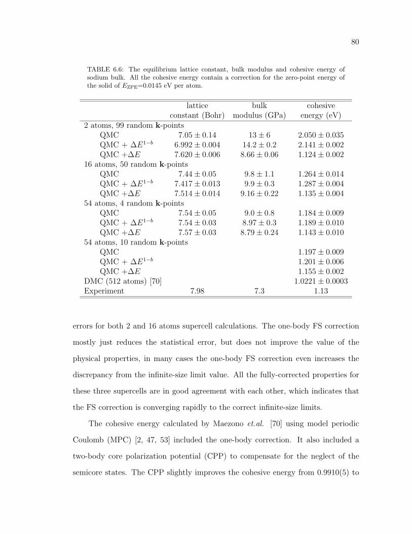
80
TABLE 6.6: The equilibrium lattice constant, bulk modulus and cohesive energy ofsodium bulk. All the cohesive energy contain a correction for the zero-point energy ofthe solid of EZPE=0.0145 eV per atom.
lattice bulk cohesiveconstant (Bohr) modulus (GPa) energy (eV)
2 atoms, 99 random k-pointsQMC 7.05± 0.14 13± 6 2.050± 0.035QMC + ∆E1−b 6.992± 0.004 14.2± 0.2 2.141± 0.002QMC +∆E 7.620± 0.006 8.66± 0.06 1.124± 0.002
16 atoms, 50 random k-pointsQMC 7.44± 0.05 9.8± 1.1 1.264± 0.014QMC + ∆E1−b 7.417± 0.013 9.9± 0.3 1.287± 0.004QMC +∆E 7.514± 0.014 9.16± 0.22 1.135± 0.004
54 atoms, 4 random k-pointsQMC 7.54± 0.05 9.0± 0.8 1.184± 0.009QMC + ∆E1−b 7.54± 0.03 8.97± 0.3 1.189± 0.010QMC +∆E 7.57± 0.03 8.79± 0.24 1.143± 0.010
54 atoms, 10 random k-pointsQMC 1.197± 0.009QMC + ∆E1−b 1.201± 0.006QMC +∆E 1.155± 0.002
DMC (512 atoms) [70] 1.0221± 0.0003Experiment 7.98 7.3 1.13
errors for both 2 and 16 atoms supercell calculations. The one-body FS correction
mostly just reduces the statistical error, but does not improve the value of the
physical properties, in many cases the one-body FS correction even increases the
discrepancy from the infinite-size limit value. All the fully-corrected properties for
these three supercells are in good agreement with each other, which indicates that
the FS correction is converging rapidly to the correct infinite-size limits.
The cohesive energy calculated by Maezono et.al. [70] using model periodic
Coulomb (MPC) [2, 47, 53] included the one-body correction. It also included a
two-body core polarization potential (CPP) to compensate for the neglect of the
semicore states. The CPP slightly improves the cohesive energy from 0.9910(5) to

81
1.0221(5) eV (the numbers in the brackets are the error in the last digit). Their 512
atom supercell calculations give a cohesive energy with an error of about 0.11 eV,
while our series of calculations using much smaller supercell of 2, 16 and 54 atoms
give consistent cohesive energies in excellent agreement with the experimental value.
6.5 Perovskite BiScO3
Perovskite structure based materials exhibit a wide range of technologically im-
portant properties such as high Tc superconductors, ferroelectricity and multiferroic
instabilities. The basic chemical formula unit is the ABO3 cubic structure, where
the A and B are cations of different sizes (for example PbTiO3 and BiScO3), the A
atom is located at the corner of the cell, the B atom is at the center, with oxygen
atoms at the face centers as the six nearest neighbor of the B atom for an octahedral
cage.
In ferroelectric materials such as BaTiO3, the cubic structure is unstable against
symmetry lowering distortion. Off-centering along the [0 0 1] direction, for example
yields a tetragonal structure, while distortions along the [1 1 1] direction produce a
rhombohedral structure. The lower symmetry structures have a net electric dipole
moment and the material is said to be ferroelectric.
The perovskite alloys of BiScO3 with PbTiO3, (BiScO3)1−x-(PbTiO3)x (BS-PT)
exhibit some interesting properties [72, 73]. The piezoelectric properties are com-
parable to the Pb(Zr1−xTix)O3 (PZT) and Pb(Zn1/3Nb2/3)O3 (PZN). BS-PT has
more robust dielectric and piezoelectric properties over a wider range of tempera-
ture, compared with PZT and PZN-PT [72–74]. First-principle studies of the end
compound, BiScO3, by Iniguez et.al. [75] using the LDA indicated an extraordinary
large well-depth of about 1 eV, compared with the well-depth of PT of 60 meV in
the tetragonal structure. It also has a large c/a = 1.29 strain in the tetragonal

82
FIG. 6.12: The ABO3 perovskite structure. Off-centering along the [0 0 1] axis gives atetragonal structure, while the off-centering along the diagonal [1 1 1] yields a rhombo-hedral structure.
phase compared with 1.05 in tetragonal PT.
The accuracy of this large ferroelectric well-depth are not readily validated by
experiment [75], and the corresponding error due to the LDA or GGA (generalized
gradient approximation) of DFT is not known. It is known that DFT using LDA
tends to systematically underestimate the equilibrium volume of perovskite by about
3% and GGA tends to overcompensate and yields volume of about 3% too large
[76]. Our aim is to use quantum Monte Carlo (QMC) calculation to probe this. The
end compound BS has a large well-depth, which reduces the required Monte Carlo
statistical accuracy.
The QMC calculations use a single Slater determinant trial wavefunction obtain
from DFT program ABINIT. Norm-conserving pseudopotential constructed using

83
OPIUM are used to remove the core electrons with a kinetic energy cutoff Ecut = 64
Ry. For the primitive BiScO3 unit cell, 44 valence electrons are included: Bi (5d10
6s2 6p3), Sc(3s2 3p6 3d1 4s2), O(2s2 2p4). Using the same structural parameters as
in Ref. [75] (see Appendix C), our pseudopotentials well-depth results are in good
agreement with those in Ref. [75], which used an ultrasoft pseudopotential. Fig. 6.13
shows the well-depths of both structures calculated using OPIUM pseudopotentials.
The present tetragonal and rhombohedral well-depths are -1.098 and -1.339 eV,
respectively, compared to -1.124 and -1.353 eV in Ref. [75]. To achieve this level
of agreement as well as small residual forces, we found it necessary to include a Bi
l = 3 pseudopotential. All calculations are with a 6 × 6 × 6 Monkhorst-Pack [50]
k-point grid.
-1.5 -1 -0.5 0 0.5 1 1.5-4496
-4495.5
-4495
-4494.5
-4494
-4493.5
-4493
-4492.5
Ene
rgy
(eV
)
∆E(R)
∆E(T)
Cubic
Tetragonal
Rhombohedral
Distortion along [0 0 1] axisDistortion along [1 1 1] axis
= -1.339 eV
=-1.098 eV
FIG. 6.13: The tetragonal and rhombohedral ferroelectric instabilities of perovskiteBiScO3 calculated with ABINIT using OPIUM pseudopotentials. The positive x axisrepresent the distortion amplitude along the [0 0 1] direction, while the negative x axisshows that along the [1 1 1] direction.
The k-point convergence of the well-depth is shown in Table 6.7. The well-

84
TABLE 6.7: The one-body size effects in DFT calculations of BiScO3. There are severalset of k-points in this table: 3 Monkhorst-Pack k-point grid calculations (2 × 2 × 2,4×4×4, and 6×6×6), the Γ-point calculation and 2 twist-averaged boundary conditionscalculations (based on 2 × 2 × 2 and 4 × 4 × 4 MP k-point grids). The well-depth oftetragonal and rhombohedral structures are in eV.
∆E(T ) ∆E(R)MP 2× 2× 2 -1.238 -1.601MP 4× 4× 4 -1.092 -1.334MP 6× 6× 6 -1.098 -1.339Γ-point -7.531 -4.385TBC 2× 2× 2 -1.238 -1.594TBC 4× 4× 4 -1.067 -1.353
depth calculations using MP 4 × 4 × 4 are already quite converged, with an error
on the order of few meV. Using TABC instead yields similar results. Using only the
Γ-point yields large one-body FS errors.
The two-body FS corrections (Table 6.8) for non-cubical structures are obtained
from the same XC function EXC(rs, L) as described in Table 5.2. Since the shapes
of both the tetragonal and rhombohedral unit cells are only slightly different from
cubic, L is defined as L = Ω1/3. The two-body FS corrections are individually large
for the primitive cubic, tetragonal and rhombohedral unit cells, which are small
in size. Table 6.8 shows the two-body FS corrections for sequences of 4 supercells
corresponding to number of atom of 5, 40, 135 and 320 atoms. The cubic simulation
cell is smallest, and therefore has the largest FS error, while the largest rhombohedral
cell has the smallest correction. The two-body FS corrections are linear with respect
to the inverse of volume for all three structures. Due to cancellation of errors,
the two-body correction for the tetragonal and rhombohedral well-depths are much
smaller than the energy corrections as shown in Table 6.8 and Fig. 6.14. However
the well-depth correction is still large for the primitive cell.
The well-depths calculated with QMC method together with the corrected QMC
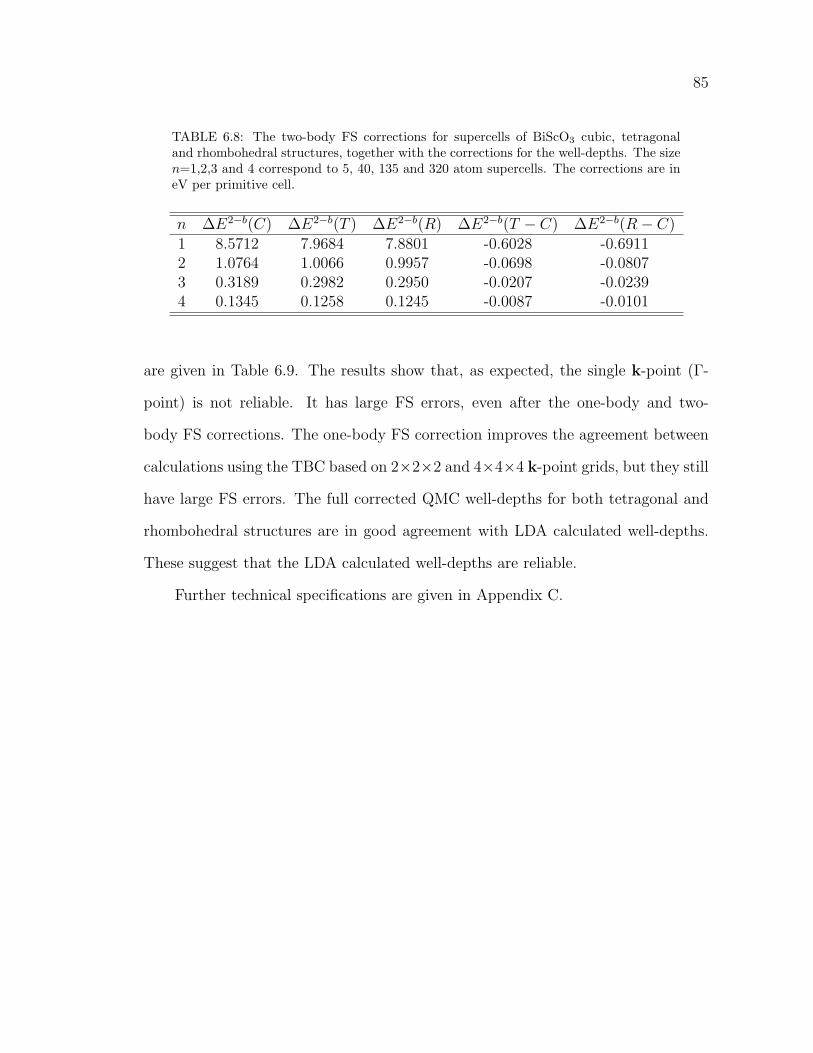
85
TABLE 6.8: The two-body FS corrections for supercells of BiScO3 cubic, tetragonaland rhombohedral structures, together with the corrections for the well-depths. The sizen=1,2,3 and 4 correspond to 5, 40, 135 and 320 atom supercells. The corrections are ineV per primitive cell.
n ∆E2−b(C) ∆E2−b(T ) ∆E2−b(R) ∆E2−b(T − C) ∆E2−b(R− C)1 8.5712 7.9684 7.8801 -0.6028 -0.69112 1.0764 1.0066 0.9957 -0.0698 -0.08073 0.3189 0.2982 0.2950 -0.0207 -0.02394 0.1345 0.1258 0.1245 -0.0087 -0.0101
are given in Table 6.9. The results show that, as expected, the single k-point (Γ-
point) is not reliable. It has large FS errors, even after the one-body and two-
body FS corrections. The one-body FS correction improves the agreement between
calculations using the TBC based on 2×2×2 and 4×4×4 k-point grids, but they still
have large FS errors. The full corrected QMC well-depths for both tetragonal and
rhombohedral structures are in good agreement with LDA calculated well-depths.
These suggest that the LDA calculated well-depths are reliable.
Further technical specifications are given in Appendix C.
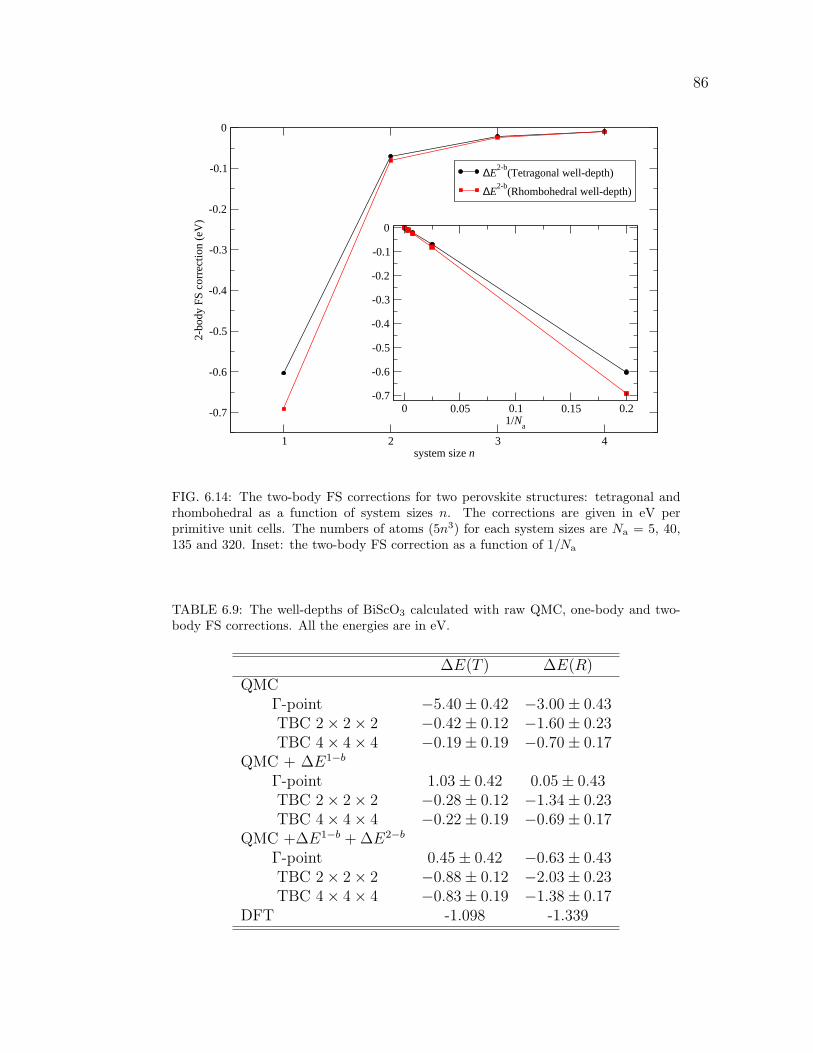
86
1 2 3 4system size n
-0.7
-0.6
-0.5
-0.4
-0.3
-0.2
-0.1
0
2-bo
dy F
S co
rrec
tion
(eV
)
∆E2-b
(Tetragonal well-depth)
∆E2-b
(Rhombohedral well-depth)
0 0.05 0.1 0.15 0.21/N
a
-0.7
-0.6
-0.5
-0.4
-0.3
-0.2
-0.1
0
FIG. 6.14: The two-body FS corrections for two perovskite structures: tetragonal andrhombohedral as a function of system sizes n. The corrections are given in eV perprimitive unit cells. The numbers of atoms (5n3) for each system sizes are Na = 5, 40,135 and 320. Inset: the two-body FS correction as a function of 1/Na
TABLE 6.9: The well-depths of BiScO3 calculated with raw QMC, one-body and two-body FS corrections. All the energies are in eV.
∆E(T ) ∆E(R)QMC
Γ-point −5.40± 0.42 −3.00± 0.43TBC 2× 2× 2 −0.42± 0.12 −1.60± 0.23TBC 4× 4× 4 −0.19± 0.19 −0.70± 0.17
QMC + ∆E1−b
Γ-point 1.03± 0.42 0.05± 0.43TBC 2× 2× 2 −0.28± 0.12 −1.34± 0.23TBC 4× 4× 4 −0.22± 0.19 −0.69± 0.17
QMC +∆E1−b + ∆E2−b
Γ-point 0.45± 0.42 −0.63± 0.43TBC 2× 2× 2 −0.88± 0.12 −2.03± 0.23TBC 4× 4× 4 −0.83± 0.19 −1.38± 0.17
DFT -1.098 -1.339
CHAPTER 7
Conclusion and Outlook
Realistic many-body calculations for extended systems are needed to accurately
treat systems where the otherwise successful density functional theory (DFT) ap-
proach fails. Effective single-particle methods such as DFT or Hartree-Fock (HF)
routinely exploit Bloch’s theorem in calculation for extended systems. In crystalline
materials, the cost of the calculation depends only on the number of atoms in the
periodic cell while the macroscopic limit is achieved by quadrature in the Brillouin
zone, using finite number of k-points. Many-body methods, in contrast, cannot
avail themselves of this simplification. Instead, calculations must be performed us-
ing increasingly larger supercells. Because the Coulomb interactions are long-ranged,
finite-size effects tend to persist to large system sizes, making reliable extrapolations
impractical.
In state-of-the-art quantum simulations, finite size (FS) errors often can be
more significant than the statistical or other systematic errors. Reducing FS errors
is thus a key to broader applications of many-body calculations in real materials.
Previous attempts have focused on estimating the FS errors internally within the
many-body simulation. In this thesis, I introduced an external correction method
87

88
which is designed to approximately include two-body FS corrections in finite-size
DFT calculations. The method is simple, and provides post-processing corrections
applicable to any previously obtained many-body results. Conceptually, it gives a
consistent framework for relating FS effects in many-body and DFT calculations,
which is important if the two methods are to be seamlessly interfaced to bridge length
scales. The correction method is applied to a model insulator (P2 in a supercell),
to semiconductor bulk silicon, to sodium metal and to perovskite BiScO3. We find
that it consistently removes most of the FS errors, leading to rapid convergence of
the many-body results to the infinite system.
The FS correction is constructed for cubic simulation cells, but the correction
is shown to be accurate for non-cubic supercells as well, including fcc cells and
ferroelectrically distorted cubic cells. The current FS functional is restricted to
systems without spin polarization but the extension to include spin polarization
should be straightforward. Including polarization will be important in treating
solids with magnetic order.
Our tests indicate that the FS correction from the Hartree-Fock method tends to
overcorrect the energy. The present DFT FS correction gives much better corrections
but they tend to be somewhat too small. Replacing the exchange energy with an
orbitally dependent exact exchange functional should be investigated, since it could
improve the quality of the correction.
Other possible future work could include further study of the shape dependence
of the FS correction for non cubic systems with extreme aspect ratios.
Finally, I have presented calculations of the cutoff energy dependence of the
correlation energy. Fitting this data to a function Ec(rs, Ecut) could be useful for
obtaining a finite-basis correction in many-body calculations. The idea is similar
to the FS correction of many-body calculations. Further studies are needed to test
these ideas.

APPENDIX A
Pseudopotential
The tightly bound core electrons of an atom are fairly insensitive to the chemical
environment of the atom. Including the core electrons can be very expensive but has
a little effect. The use of a pseudopotential eliminates the core electron states from
the spectrum of the valence-only pseudo-Hamiltonian, while retaining an accurate
description of valence electron bounding.
Norm conserving Kleinman-Bylander type non local pseudopotentials [31] are
used in this thesis. The requirements for a good norm-conserving pseudopotential
are given by Hamann, Schluter and Chiang [77]:
1. All-electron and pseudo valence eigenvalues agree for the chosen atomic reference
configuration.
2. All-electron and pseudo valence wavefunction agree beyond a chosen core radius
rc.
3. The integrated charge inside a radius rc from the nucleus for each wavefunction
agrees (norm-conservation) with the all-electron value.
4. The logarithmic derivatives of all electron and pseudo wavefunction agree at
89

90
rc (this reproduces the valence electron scattering properties near the reference
energy).
5. The first energy derivatives of the logarithmic derivatives of the all-electron and
pseudo wavefunctions agrees at rc.
It is useful to separate the ionic pseudopotential into a local (l-independent)
part
〈r|V loc|r′〉 = V loc(r)δ(r− r′), (A.1)
and semi local (l-dependent) part.
〈r|V nl|r′〉 = V nl(r, r′). (A.2)
In the following discussion, I describe the applications of the pseudopotential in
calculations using periodic boundary condition.
Let first consider the local potential. The local potential is given as a sum over
all ion’s contributions in a crystal:
V loc(r) =∑R,α
V locα (|r− dα −R|), (A.3)
where R is the direct lattice vector, and dα is the relative position of the α atom
in a simulation cell relative to the cell’s origin. The sum over R is an infinite sum,
since a crystal is perfectly periodic over all spaces. The matrix element of this local
potential in reciprocal space is given by
〈k + G|V loc|k + G′〉 =1
V∑R,α
∫d3re−i(G−G′)·rV loc
α (r− dα −R). (A.4)
Note that in this expression, there is no k-vector dependence. Now let us define

91
r′ ≡ r− dα −R. Then the matrix element becomes
〈k + G|V loc|k + G′〉 =1
V∑R,α
e−i(G−G′)·(dα+R)
∫d3r′e−i(G−G′)·r′
V locα (r′)
=1
Ω
∑α
e−i(G−G′)·dαV locα (G−G′)
≡ V loc(G−G′) (A.5)
We have used the fact that ei(G−G′)·R = 1 for any direct lattice vector R, and that
V−1∑
R = Ω−1. The terms V locα , defined as
V locα (Q) =
∫d3re−iQ·rV loc
α (r), (A.6)
are simply the Fourier transform of the local potential. Using the planewave expan-
sion [78]
eik.r = 4π∞∑l=0
iljl(kr)l∑
m=−l
Y ∗l,m(k)Yl,m(r), (A.7)
together with the orthogonality of the spherical harmonic Yl,m(θ, φ), Eq. (A.6) can
be simplified:
V locα (Q) = 4π
∫ ∞0
r2j0(Qr)Vα(r)dr (A.8)
where j0(Qr) is a spherical Bessel function. This function is obtained directly from
pseudopotential code. It is convenient to add and subtract the long range point
charge Coulomb potential with effective charge equal to +Zval so that the local
potential has a rapid spatial decay. The point charge term is handle in Fourier
space: ∫d3reiQ·r
+Zα|r|
=4πZα|Q|2
. (A.9)
Due to charge neutrality, the divergent Q = 0 term cancels between electron-ion,
electron-electron and ion-ion interactions.

92
Similarly, the nonlocal pseudopotential is given by:
V nl =∑R,α
V nlα (r− dα −R, r′ − dα −R). (A.10)
Using the same manipulation as above, the matrix element is given by
〈k + G|V nl|k + G′〉
=1
V
∫d3rd3r′e−i(k+G).r
(∑R,α
V nlα (r− dα −R, r′ − dα −R)
)e−i(k+G′).r′
=1
Ω
∑α
e−i(G−G′).dαV nlα (k + G,k + G′).
≡ V nl(k + G,k + G′) (A.11)
This form is expensive to use in calculations. The Kleinman-Bylander fully non-local
pseudopotential [31] is given in the following separate form:
V nlα =
∑l,m
|Vα,lϕpsα,lYl,m〉〈Yl,mϕ
psα,lVα,l|
ηα,l(A.12)
where
ηα,l = 〈Yl,mϕpsα,l|Vα,l|ϕ
psα,lYl,m〉. (A.13)
Substitute Eq. (A.12) into Eq. (A.11), we get:
V nlα (Q,Q′) =
∑l,m
1
ηα,l
∫d3re−iQ.rVα,l(r)ϕ
psα,l(r)Yl,m(r)∫
d3r′e−iQ′.r′Vα,l(r
′)ϕpsα,l(r
′)Yl,m(r′) (A.14)
Obviously this two integrations are identical and separable. Let evaluate one of
them:
I(Q) =
∫d3re−iQ.rVα,l(r)ϕ
psα,l(r)Yl,m(r)
= 4π∑l′
(−i)l′∫r2drdΩjl′(Qr)
l′∑m′=−l′
Yl′,m′(Q)Y ∗l′,m′(r)Vα,l(r)ϕpsα,l(r)Yl.m(r)
= 4π(−i)l∫r2drjl(Qr)Vα,l(r)ϕ
psα,lYl,m(Q) (A.15)

93
In the last equation, we use the orthogonality of the spherical harmonics. Now let
us define:
fα,l(Q) =
∫r2drjl(Qr)Vα,l(r)ϕ
psα,l. (A.16)
This function is obtained directly from pseudopotential code. Then Eq. (A.11) can
be written as:
〈Q|V nl|Q′〉 =(4π)2
Ω
∑l,m
1
ηα,l
∑α
e−i(Q−Q′).dαfα,l(Q)Yl,m(Q)fα,l(Q′)Yl,m(Q′), (A.17)
where Q = k + G and Q′ = k + G′. Defining
Fj(Q) ≡ Fα,l,m(Q) ≡ 4π√ΩeiQ.dαfα,l(Q)Y ∗l,m(Q′), (A.18)
the nonlocal matrix element takes a simple separable form:
〈k + G|V nl|k + G′〉 =∑
j∈(α,l,m)
1
ηjF ∗j (k + G)Fj(k + G′). (A.19)
This is the form used in planewave base DFT calculations and in our planewave
AFQMC code.

APPENDIX B
Dependence of the Jellium
Correlation Energy on the Cutoff
Energy Ecut
The jellium system is described in Chapter 4. A series of calculations were
performed using AFQMC method in cubic simulation cells with no spin polarization
with N electrons. There are total of 25 sets of data for densities of rs= 1, 2, 3, 4,
and 5 Bohr. For each density, calculations were performed with N equal to 10, 20,
30, 40 and 50 electrons. Each set was obtained from TABC averages over 20 QMC
calculations with different k-points [52]. The results of over 5000 calculations are
presented in the five tables below.
The cutoff energy is expressed as a function of the Fermi energy (as given by
restricted HF). The Fermi momentum is given by Eq. (4.7),
kF =
(9π
4
) 13 1
rs, (B.1)
94

95
and the Fermi energy is given by
EF =~2k2
F
2m, (B.2)
only depends on the density of the system. The relation between the cube edge L,
the number of electrons N , and the density rs is given in Eq. (4.2)
L = rs
(4πN
3
) 13
. (B.3)
The Fermi energy definition given here is for the infinite size limit. In finite size
simulations, EF has a k-point dependence. For example, in the system of 54 elec-
trons using the Γ-point, the electrons fill the momentum states G = (0,0,0), (1,0,0),
(1,1,0) and (1,1,1) (and all other states related with these 4 states by symmetry) in
units of 2πL
. The electrons with highest energy fill the G = (1, 1, 1) state. The Fermi
momentum of this electron is kF =√(
2πL
)2(12 + 12 + 12) = 2π
L
√3 = 1.7322π
L. The
Fermi momentum calculated with Eq. (B.1) is 2πL
(814π
)1/3= 1.8612π
L. In the limit
of large simulation cells with a large number of particles, the approximate formula
is equal to the exact result. Moreover, the average of Fermi momenta over many
k-points also tends to the result in Eq. (B.1).
The correlation energy is given as the difference between the total energy and
the Hartree-Fock energy. The HF energy is independent of the size of the basis, as
long as the basis is large enough to accommodate all electrons. When the basis size
exactly accommodate the number of electrons, the HF energy is exactly the same
with the AFQMC total energy so the correlation energy is exactly zero in this case.
The list of random k-points used in the simulations is given in Table B.1. Since
the QMC statistical error is much smaller than the error due to k-point averaging
(by approximately two orders of magnitude), the errors reported here are from the
k-point averaging only. The Hartree-Fock energy, by definition, does not have a
statistical error, but it still has a k-point averaging error. As expected, the error in

96
TABLE B.1: The list of k-points used in the simulation in reduced coordinate2πL (kx, ky, kz).
kx ky kz1 0.0506 0.1980 0.27002 0.1764 0.1229 0.41073 0.2489 0.2204 0.00654 0.2690 0.4449 0.49215 0.2952 0.3266 0.24466 0.2011 0.0913 0.39787 0.3071 0.0455 0.04578 0.4285 0.2451 0.11159 0.4449 0.0281 0.409510 0.1301 0.1981 0.281011 0.3360 0.0695 0.317012 0.1185 0.2152 0.050213 0.2379 0.0838 0.224414 0.0122 0.3499 0.442015 0.2693 0.1890 0.208616 0.4659 0.2727 0.426017 0.1087 0.4740 0.101118 0.2392 0.3505 0.195519 0.3802 0.3269 0.171620 0.4423 0.3462 0.4634
HF is correlated with that in QMC, so the correlation energy has a much smaller
error. All energies reported here are in Rydberg atomic units.
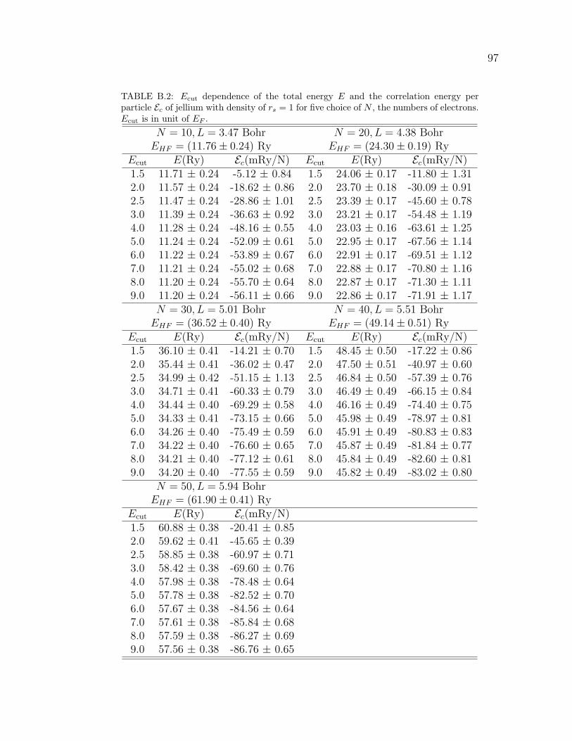
97
TABLE B.2: Ecut dependence of the total energy E and the correlation energy perparticle Ec of jellium with density of rs = 1 for five choice of N , the numbers of electrons.Ecut is in unit of EF .
N = 10, L = 3.47 Bohr N = 20, L = 4.38 BohrEHF = (11.76± 0.24) Ry EHF = (24.30± 0.19) Ry
Ecut E(Ry) Ec(mRy/N) Ecut E(Ry) Ec(mRy/N)1.5 11.71 ± 0.24 -5.12 ± 0.84 1.5 24.06 ± 0.17 -11.80 ± 1.312.0 11.57 ± 0.24 -18.62 ± 0.86 2.0 23.70 ± 0.18 -30.09 ± 0.912.5 11.47 ± 0.24 -28.86 ± 1.01 2.5 23.39 ± 0.17 -45.60 ± 0.783.0 11.39 ± 0.24 -36.63 ± 0.92 3.0 23.21 ± 0.17 -54.48 ± 1.194.0 11.28 ± 0.24 -48.16 ± 0.55 4.0 23.03 ± 0.16 -63.61 ± 1.255.0 11.24 ± 0.24 -52.09 ± 0.61 5.0 22.95 ± 0.17 -67.56 ± 1.146.0 11.22 ± 0.24 -53.89 ± 0.67 6.0 22.91 ± 0.17 -69.51 ± 1.127.0 11.21 ± 0.24 -55.02 ± 0.68 7.0 22.88 ± 0.17 -70.80 ± 1.168.0 11.20 ± 0.24 -55.70 ± 0.64 8.0 22.87 ± 0.17 -71.30 ± 1.119.0 11.20 ± 0.24 -56.11 ± 0.66 9.0 22.86 ± 0.17 -71.91 ± 1.17
N = 30, L = 5.01 Bohr N = 40, L = 5.51 BohrEHF = (36.52± 0.40) Ry EHF = (49.14± 0.51) Ry
Ecut E(Ry) Ec(mRy/N) Ecut E(Ry) Ec(mRy/N)1.5 36.10 ± 0.41 -14.21 ± 0.70 1.5 48.45 ± 0.50 -17.22 ± 0.862.0 35.44 ± 0.41 -36.02 ± 0.47 2.0 47.50 ± 0.51 -40.97 ± 0.602.5 34.99 ± 0.42 -51.15 ± 1.13 2.5 46.84 ± 0.50 -57.39 ± 0.763.0 34.71 ± 0.41 -60.33 ± 0.79 3.0 46.49 ± 0.49 -66.15 ± 0.844.0 34.44 ± 0.40 -69.29 ± 0.58 4.0 46.16 ± 0.49 -74.40 ± 0.755.0 34.33 ± 0.41 -73.15 ± 0.66 5.0 45.98 ± 0.49 -78.97 ± 0.816.0 34.26 ± 0.40 -75.49 ± 0.59 6.0 45.91 ± 0.49 -80.83 ± 0.837.0 34.22 ± 0.40 -76.60 ± 0.65 7.0 45.87 ± 0.49 -81.84 ± 0.778.0 34.21 ± 0.40 -77.12 ± 0.61 8.0 45.84 ± 0.49 -82.60 ± 0.819.0 34.20 ± 0.40 -77.55 ± 0.59 9.0 45.82 ± 0.49 -83.02 ± 0.80
N = 50, L = 5.94 BohrEHF = (61.90± 0.41) Ry
Ecut E(Ry) Ec(mRy/N)1.5 60.88 ± 0.38 -20.41 ± 0.852.0 59.62 ± 0.41 -45.65 ± 0.392.5 58.85 ± 0.38 -60.97 ± 0.713.0 58.42 ± 0.38 -69.60 ± 0.764.0 57.98 ± 0.38 -78.48 ± 0.645.0 57.78 ± 0.38 -82.52 ± 0.706.0 57.67 ± 0.38 -84.56 ± 0.647.0 57.61 ± 0.38 -85.84 ± 0.688.0 57.59 ± 0.38 -86.27 ± 0.699.0 57.56 ± 0.38 -86.76 ± 0.65

98
TABLE B.3: Ecut dependence of the total energy E and the correlation energy perparticle Ec of jellium with density of rs = 2 for five choice of N , the numbers of electrons.Ecut is in unit of EF .
N = 10, L = 6.95 Bohr N = 20, L = 8.75 BohrEHF = (0.233± 0.064) Ry EHF = (0.960± 0.057) Ry
Ecut E(Ry) Ec(mRy/N) Ecut E(Ry) Ec(mRy/N)1.5 0.187 ± 0.063 -4.56 ± 0.74 1.5 0.768 ± 0.043 -9.63 ± 1.012.0 0.068 ± 0.063 -16.48 ± 0.77 2.0 0.470 ± 0.052 -24.49 ± 0.652.5 -0.021 ± 0.061 -25.34 ± 0.79 2.5 0.222 ± 0.051 -36.93 ± 0.493.0 -0.086 ± 0.064 -31.89 ± 0.78 3.0 0.067 ± 0.043 -44.68 ± 0.844.0 -0.188 ± 0.062 -42.10 ± 0.52 4.0 -0.103 ± 0.043 -53.16 ± 0.875.0 -0.222 ± 0.061 -45.45 ± 0.45 5.0 -0.173 ± 0.045 -56.65 ± 0.746.0 -0.237 ± 0.061 -46.97 ± 0.49 6.0 -0.205 ± 0.044 -58.24 ± 0.737.0 -0.246 ± 0.060 -47.88 ± 0.55 7.0 -0.221 ± 0.045 -59.07 ± 0.758.0 -0.251 ± 0.061 -48.36 ± 0.44 8.0 -0.224 ± 0.045 -59.20 ± 0.779.0 -0.251 ± 0.060 -48.38 ± 0.50 9.0 -0.240 ± 0.044 -59.99 ± 0.82
N = 30, L = 10.02 Bohr N = 40, L = 11.03 BohrEHF = (1.624± 0.099) Ry EHF = (2.418± 0.138) Ry
Ecut E(Ry) Ec(mRy/N) Ecut E(Ry) Ec(mRy/N)1.5 1.282 ± 0.109 -11.41 ± 0.51 1.5 1.885 ± 0.132 -13.34 ± 0.632.0 0.769 ± 0.104 -28.51 ± 0.35 2.0 1.162 ± 0.142 -31.41 ± 0.452.5 0.410 ± 0.114 -40.46 ± 0.85 2.5 0.620 ± 0.132 -44.95 ± 0.483.0 0.161 ± 0.108 -48.76 ± 0.60 3.0 0.320 ± 0.125 -52.46 ± 0.464.0 -0.081 ± 0.103 -56.84 ± 0.38 4.0 0.009 ± 0.128 -60.24 ± 0.425.0 -0.191 ± 0.105 -60.50 ± 0.48 5.0 -0.151 ± 0.127 -64.24 ± 0.456.0 -0.250 ± 0.103 -62.46 ± 0.34 6.0 -0.228 ± 0.123 -66.16 ± 0.567.0 -0.279 ± 0.104 -63.45 ± 0.47 7.0 -0.261 ± 0.123 -66.97 ± 0.488.0 -0.285 ± 0.101 -63.63 ± 0.41 8.0 -0.279 ± 0.125 -67.43 ± 0.499.0 -0.302 ± 0.103 -64.19 ± 0.42 9.0 -0.289 ± 0.123 -67.70 ± 0.50
N = 50, L = 11.88 BohrEHF = (3.262± 0.115) Ry
Ecut E(Ry) Ec(mRy/N)1.5 2.492 ± 0.092 -15.42 ± 0.592.0 1.524 ± 0.116 -34.76 ± 0.292.5 0.908 ± 0.101 -47.09 ± 0.393.0 0.543 ± 0.096 -54.39 ± 0.434.0 0.127 ± 0.101 -62.71 ± 0.375.0 -0.075 ± 0.099 -66.75 ± 0.426.0 -0.142 ± 0.099 -68.08 ± 0.417.0 -0.200 ± 0.099 -69.25 ± 0.418.0 -0.223 ± 0.097 -69.72 ± 0.429.0 -0.246 ± 0.100 -70.17 ± 0.38

99
TABLE B.4: Ecut dependence of the total energy E and the correlation energy perparticle Ec of jellium with density of rs = 3 for five choice of N , the numbers of electrons.Ecut is in unit of EF .
N = 10, L = 10.42 Bohr N = 20, L = 13.13 BohrEHF = (−1.099± 0.030) Ry EHF = (−1.846± 0.030) Ry
Ecut E(Ry) Ec(mRy/N) Ecut E(Ry) Ec(mRy/N)1.5 -1.141 ± 0.029 -4.14 ± 0.69 1.5 -2.010 ± 0.018 -8.19 ± 0.862.0 -1.246 ± 0.029 -14.63 ± 0.68 2.0 -2.257 ± 0.026 -20.54 ± 0.532.5 -1.321 ± 0.026 -22.18 ± 0.75 2.5 -2.465 ± 0.025 -30.93 ± 0.413.0 -1.380 ± 0.030 -28.08 ± 0.62 3.0 -2.600 ± 0.019 -37.70 ± 0.674.0 -1.469 ± 0.030 -36.92 ± 0.37 4.0 -2.750 ± 0.019 -45.19 ± 0.645.0 -1.501 ± 0.028 -40.13 ± 0.40 5.0 -2.817 ± 0.022 -48.53 ± 0.516.0 -1.518 ± 0.027 -41.87 ± 0.50 6.0 -2.842 ± 0.021 -49.78 ± 0.567.0 -1.523 ± 0.028 -42.35 ± 0.35 7.0 -2.867 ± 0.017 -51.05 ± 0.728.0 -1.524 ± 0.028 -42.47 ± 0.39 8.0 -2.873 ± 0.020 -51.34 ± 0.619.0 -1.526 ± 0.028 -42.67 ± 0.39 9.0 -2.879 ± 0.020 -51.63 ± 0.60
N = 30, L = 15.03 Bohr N = 40, L = 16.54 BohrEHF = (−2.614± 0.044) Ry EHF = (−3.310± 0.066) Ry
Ecut E(Ry) Ec(mRy/N) Ecut E(Ry) Ec(mRy/N)1.5 -2.897 ± 0.052 -9.42 ± 0.39 1.5 -3.745 ± 0.061 -10.87 ± 0.482.0 -3.325 ± 0.048 -23.69 ± 0.26 2.0 -4.337 ± 0.070 -25.66 ± 0.352.5 -3.639 ± 0.058 -34.15 ± 0.70 2.5 -4.786 ± 0.066 -36.90 ± 0.293.0 -3.839 ± 0.051 -40.82 ± 0.38 3.0 -5.062 ± 0.057 -43.79 ± 0.334.0 -4.069 ± 0.048 -48.50 ± 0.35 4.0 -5.342 ± 0.062 -50.79 ± 0.305.0 -4.162 ± 0.049 -51.60 ± 0.36 5.0 -5.497 ± 0.058 -54.66 ± 0.326.0 -4.212 ± 0.048 -53.25 ± 0.29 6.0 -5.546 ± 0.058 -55.90 ± 0.337.0 -4.236 ± 0.046 -54.05 ± 0.24 7.0 -5.578 ± 0.059 -56.70 ± 0.298.0 -4.249 ± 0.048 -54.48 ± 0.28 8.0 -5.606 ± 0.061 -57.39 ± 0.339.0 -4.261 ± 0.047 -54.89 ± 0.28 9.0 -5.612 ± 0.055 -57.55 ± 0.37
N = 50, L = 17.82 BohrEHF = (−3.978± 0.057) Ry
Ecut E(Ry) Ec(mRy/N)1.5 -4.602 ± 0.039 -12.48 ± 0.462.0 -5.377 ± 0.061 -27.97 ± 0.212.5 -5.907 ± 0.046 -38.58 ± 0.323.0 -6.245 ± 0.041 -45.33 ± 0.404.0 -6.626 ± 0.049 -52.96 ± 0.285.0 -6.801 ± 0.046 -56.46 ± 0.356.0 -6.877 ± 0.047 -57.97 ± 0.337.0 -6.909 ± 0.048 -58.62 ± 0.268.0 -6.935 ± 0.045 -59.14 ± 0.339.0 -6.938 ± 0.047 -59.20 ± 0.23
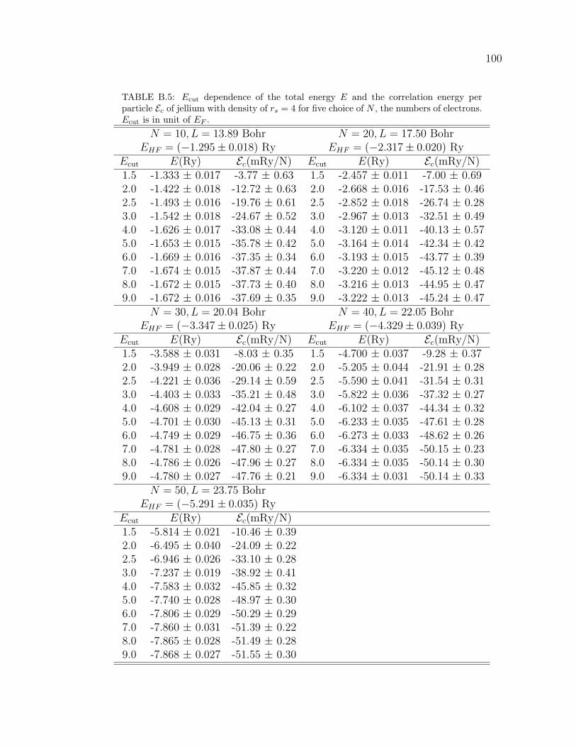
100
TABLE B.5: Ecut dependence of the total energy E and the correlation energy perparticle Ec of jellium with density of rs = 4 for five choice of N , the numbers of electrons.Ecut is in unit of EF .
N = 10, L = 13.89 Bohr N = 20, L = 17.50 BohrEHF = (−1.295± 0.018) Ry EHF = (−2.317± 0.020) Ry
Ecut E(Ry) Ec(mRy/N) Ecut E(Ry) Ec(mRy/N)1.5 -1.333 ± 0.017 -3.77 ± 0.63 1.5 -2.457 ± 0.011 -7.00 ± 0.692.0 -1.422 ± 0.018 -12.72 ± 0.63 2.0 -2.668 ± 0.016 -17.53 ± 0.462.5 -1.493 ± 0.016 -19.76 ± 0.61 2.5 -2.852 ± 0.018 -26.74 ± 0.283.0 -1.542 ± 0.018 -24.67 ± 0.52 3.0 -2.967 ± 0.013 -32.51 ± 0.494.0 -1.626 ± 0.017 -33.08 ± 0.44 4.0 -3.120 ± 0.011 -40.13 ± 0.575.0 -1.653 ± 0.015 -35.78 ± 0.42 5.0 -3.164 ± 0.014 -42.34 ± 0.426.0 -1.669 ± 0.016 -37.35 ± 0.34 6.0 -3.193 ± 0.015 -43.77 ± 0.397.0 -1.674 ± 0.015 -37.87 ± 0.44 7.0 -3.220 ± 0.012 -45.12 ± 0.488.0 -1.672 ± 0.015 -37.73 ± 0.40 8.0 -3.216 ± 0.013 -44.95 ± 0.479.0 -1.672 ± 0.016 -37.69 ± 0.35 9.0 -3.222 ± 0.013 -45.24 ± 0.47
N = 30, L = 20.04 Bohr N = 40, L = 22.05 BohrEHF = (−3.347± 0.025) Ry EHF = (−4.329± 0.039) Ry
Ecut E(Ry) Ec(mRy/N) Ecut E(Ry) Ec(mRy/N)1.5 -3.588 ± 0.031 -8.03 ± 0.35 1.5 -4.700 ± 0.037 -9.28 ± 0.372.0 -3.949 ± 0.028 -20.06 ± 0.22 2.0 -5.205 ± 0.044 -21.91 ± 0.282.5 -4.221 ± 0.036 -29.14 ± 0.59 2.5 -5.590 ± 0.041 -31.54 ± 0.313.0 -4.403 ± 0.033 -35.21 ± 0.48 3.0 -5.822 ± 0.036 -37.32 ± 0.274.0 -4.608 ± 0.029 -42.04 ± 0.27 4.0 -6.102 ± 0.037 -44.34 ± 0.325.0 -4.701 ± 0.030 -45.13 ± 0.31 5.0 -6.233 ± 0.035 -47.61 ± 0.286.0 -4.749 ± 0.029 -46.75 ± 0.36 6.0 -6.273 ± 0.033 -48.62 ± 0.267.0 -4.781 ± 0.028 -47.80 ± 0.27 7.0 -6.334 ± 0.035 -50.15 ± 0.238.0 -4.786 ± 0.026 -47.96 ± 0.27 8.0 -6.334 ± 0.035 -50.14 ± 0.309.0 -4.780 ± 0.027 -47.76 ± 0.21 9.0 -6.334 ± 0.031 -50.14 ± 0.33
N = 50, L = 23.75 BohrEHF = (−5.291± 0.035) Ry
Ecut E(Ry) Ec(mRy/N)1.5 -5.814 ± 0.021 -10.46 ± 0.392.0 -6.495 ± 0.040 -24.09 ± 0.222.5 -6.946 ± 0.026 -33.10 ± 0.283.0 -7.237 ± 0.019 -38.92 ± 0.414.0 -7.583 ± 0.032 -45.85 ± 0.325.0 -7.740 ± 0.028 -48.97 ± 0.306.0 -7.806 ± 0.029 -50.29 ± 0.297.0 -7.860 ± 0.031 -51.39 ± 0.228.0 -7.865 ± 0.028 -51.49 ± 0.289.0 -7.868 ± 0.027 -51.55 ± 0.30

101
TABLE B.6: Ecut dependence of the total energy E and the correlation energy perparticle Ec of jellium with density of rs = 5 for five choice of N , the numbers of electrons.Ecut is in unit of EF .
N = 10, L = 17.36 Bohr N = 20, L = 21.88 BohrEHF = (−1.262± 0.012) Ry EHF = (−2.301± 0.014) Ry
Ecut E(Ry) Ec(mRy/N) Ecut E(Ry) Ec(mRy/N)1.5 -1.296 ± 0.012 -3.42 ± 0.59 1.5 -2.423 ± 0.008 -6.09 ± 0.602.0 -1.377 ± 0.012 -11.49 ± 0.53 2.0 -2.610 ± 0.013 -15.43 ± 0.372.5 -1.436 ± 0.010 -17.37 ± 0.69 2.5 -2.771 ± 0.014 -23.49 ± 0.263.0 -1.485 ± 0.012 -22.34 ± 0.44 3.0 -2.874 ± 0.010 -28.62 ± 0.364.0 -1.555 ± 0.014 -29.29 ± 0.39 4.0 -3.004 ± 0.008 -35.15 ± 0.475.0 -1.586 ± 0.011 -32.38 ± 0.32 5.0 -3.059 ± 0.011 -37.88 ± 0.366.0 -1.595 ± 0.009 -33.34 ± 0.42 6.0 -3.082 ± 0.010 -39.02 ± 0.447.0 -1.600 ± 0.011 -33.76 ± 0.31 7.0 -3.102 ± 0.011 -40.03 ± 0.348.0 -1.602 ± 0.010 -34.04 ± 0.34 8.0 -3.113 ± 0.009 -40.61 ± 0.409.0 -1.606 ± 0.010 -34.45 ± 0.32 9.0 -3.108 ± 0.010 -40.31 ± 0.42
N = 30, L = 25.04 Bohr N = 40, L = 27.56 BohrEHF = (−3.343± 0.016) Ry EHF = (−4.349± 0.027) Ry
Ecut E(Ry) Ec(mRy/N) Ecut E(Ry) Ec(mRy/N)1.5 -3.552 ± 0.021 -6.95 ± 0.29 1.5 -4.665 ± 0.025 -7.91 ± 0.352.0 -3.869 ± 0.020 -17.54 ± 0.23 2.0 -5.108 ± 0.032 -18.98 ± 0.262.5 -4.115 ± 0.027 -25.72 ± 0.54 2.5 -5.464 ± 0.027 -27.88 ± 0.303.0 -4.282 ± 0.024 -31.30 ± 0.40 3.0 -5.656 ± 0.024 -32.68 ± 0.264.0 -4.468 ± 0.021 -37.49 ± 0.37 4.0 -5.898 ± 0.026 -38.73 ± 0.315.0 -4.547 ± 0.019 -40.13 ± 0.28 5.0 -6.029 ± 0.026 -42.01 ± 0.256.0 -4.594 ± 0.019 -41.69 ± 0.35 6.0 -6.081 ± 0.029 -43.30 ± 0.267.0 -4.625 ± 0.016 -42.73 ± 0.24 7.0 -6.119 ± 0.024 -44.26 ± 0.258.0 -4.633 ± 0.017 -43.00 ± 0.22 8.0 -6.137 ± 0.020 -44.71 ± 0.279.0 -4.633 ± 0.017 -43.01 ± 0.24 9.0 -6.129 ± 0.026 -44.50 ± 0.25
N = 50, L = 29.69 BohrEHF = (−5.340± 0.025) Ry
Ecut E(Ry) Ec(mRy/N)1.5 -5.784 ± 0.014 -8.86 ± 0.322.0 -6.372 ± 0.028 -20.64 ± 0.202.5 -6.785 ± 0.018 -28.89 ± 0.273.0 -7.028 ± 0.017 -33.75 ± 0.374.0 -7.377 ± 0.021 -40.74 ± 0.355.0 -7.526 ± 0.019 -43.70 ± 0.386.0 -7.568 ± 0.022 -44.56 ± 0.327.0 -7.622 ± 0.014 -45.64 ± 0.298.0 -7.654 ± 0.027 -46.27 ± 0.279.0 -7.653 ± 0.019 -46.25 ± 0.25

APPENDIX C
Technical Details of the BiScO3
Calculation
TABLE C.1: Structural data of BiScO3 cubic, tetragonal and rhombohedral structure (inunit of Bohr). The reduced coordinates of the tetragonal and rhombohedral structuresare given as the difference from the ideal cubic positions. Structures are from Ref. [75].
cubic tetragonal rhombohedralReal space primitive vector
R
a1 0 00 a1 00 0 a1
a2 0 00 a2 00 0 c2
a3 b3 b3
b3 a3 b3
b3 b3 a3
a1 = 7.533
a2 = 7.11284 a3 = 7.7778225c2 = 9.14 b3 = 0.0941625
Reduced coordinates of the atoms in the primitive cellBi (0.0, 0.0, 0.0) (0, 0, 0) (δr1, δr1, δr1)Sc (0.5, 0.5, 0.5) (0, 0, δt1) (δr2, δr2, δr2)O 1 (0.0, 0.5, 0.5) (0, 0, δt2) (δr3, δr4, δr4 )O 2 (0.5, 0.0, 0.5) (0, 0, δt2) (δr4, δr3, δr4 )O 3 (0.5, 0.5, 0.0) (0, 0, δt3) (δr4, δr4, δr3 )
δt1 = 0.073 δr1 = 0.0849720646δt2 = 0.229 δr2 = 0.0000032952δt3 = 0.177 δr3 = −0.0183029402
δr4 = −0.0547217723
102

103
TABLE C.2: Calculated energies of BiScO3 cubic, tetragonal and rhombohedral struc-tures. All energies are given in eV. The k-points are given in reduced coordinates. w isthe weight of each k-point
k-point w QMC DFT FS DFTCubic
( 0 0 0) −4477.17± 0.25 -4485.79 -4494.32TBC 2× 2× 2
(1/4 1/4 1/4) 1 −4488.21± 0.07 -4494.02 -4502.58TBC 4× 4× 4
(1/8 1/8 1/8) 1/8 −4483.20± 0.34 -4488.94 -4497.49(3/8 1/8 1/8) 1/8 −4486.08± 0.25 -4491.65 -4500.21(3/8 3/8 1/8) 1/8 −4490.66± 0.18 -4496.46 -4505.04(3/8 3/8 3/8) 1/8 −4495.16± 0.31 -4501.30 -4509.88
Tetragonal( 0 0 0) −4482.57± 0.34 -4493.32 -4501.26TBC 2× 2× 2
(1/4 1/4 1/4) 1 −4488.64± 0.09 -4495.26 -4503.22TBC 4× 4× 4
(1/8 1/8 1/8) 1/8 −4487.37± 0.33 -4493.94 -4501.90(3/8 1/8 1/8) 1/4 −4488.48± 0.27 -4494.90 -4502.86(3/8 3/8 1/8) 1/8 −4490.66± 0.38 -4496.75 -4504.73(1/8 1/8 3/8) 1/8 −4486.82± 0.36 -4493.71 -4501.66(3/8 1/8 3/8) 1/4 −4489.11± 0.33 -4495.60 -4503.56(3/8 3/8 3/8) 1/8 −4490.12± 0.23 -4497.71 -4505.69
Rhombohedral( 0 0 0) −4480.17± 0.36 -4490.18 -4498.03TBC 2× 2× 2
(1/4 1/4 1/4) 1/4 −4489.26± 0.08 -4495.57 -4503.43(-1/4 1/4 1/4) 3/4 −4489.99± 0.29 -4495.64 -4503.51
TBC 4× 4× 4(1/8 1/8 1/8) 1/32 −4485.52± 0.33 -4492.04 -4499.91(3/8 1/8 1/8) 3/32 −4487.34± 0.31 -4494.31 -4502.18(-3/8 1/8 1/8) 3/32 −4488.36± 0.37 -4494.24 -4502.11(-1/8 1/8 1/8) 3/32 −4485.70± 0.39 -4491.89 -4499.76(3/8 3/8 1/8) 3/32 −4490.86± 0.26 -4496.97 -4504.85(-3/8 3/8 1/8) 3/16 −4490.77± 0.30 -4497.03 -4504.92(-1/8 3/8 1/8) 3/16 −4487.82± 0.38 -4494.30 -4502.17(-3/8 -3/8 1/8) 3/32 −4491.03± 0.24 -4497.05 -4504.93(3/8 3/8 3/8) 1/32 −4492.62± 0.25 -4499.46 -4507.35(-3/8 3/8 3/8) 3/32 −4492.39± 0.24 -4499.58 -4507.48
BIBLIOGRAPHY
[1] W. M. C. Foulkes, L. Mitas, R. J. Needs, and G. Rajagopal, Rev. Mod. Phys.
73, 33 (2001).
[2] L. M. Fraser, W. M. C. Foulkes, G. Rajagopal, R. J. Needs, S. D. Kenny, and
A. J. Williamson, Phys. Rev. B 53, 1814 (1996).
[3] H. Kwee, S. Zhang and H. Krakauer (2007), submitted to Phys. Rev. Lett.,
available at http://arxiv.org/abs/0711.0921.
[4] R. M. Martin, Electronic Structure: Basic Theory and Practical Methods (Cam-
bridge University Press, 2004).
[5] A. Szabo and N. S. Ostlund, Modern Quantum Chemistry: Introduction to
Advanced Electronic Structure Theory (Dover Publications, 1996).
[6] P. Hohenberg and W. Kohn, Phys. Rev. 136, B864 (1964).
[7] W. Kohn, Rev. Mod. Phys. 71, 1253 (1999).
[8] W. Kohn and L. J. Sham, Phys. Rev. 140, A1133 (1965).
[9] D. M. Ceperley and B. J. Alder, Phys. Rev. Lett. 45, 566 (1980).
[10] J. P. Perdew and A. Zunger, Phys. Rev. B 23, 5048 (1981).
[11] R. O. Jones and O. Gunnarsson, Rev. Mod. Phys. 61, 689 (1989).
104
105
[12] A. J. Williamson, R. Q. Hood, and J. C. Grossman, Phys. Rev. Lett. 87, 246406
(2001).
[13] S. Fahy, X. W. Wang, and S. G. Louie, Phys. Rev. B 42, 3503 (1990).
[14] S. Zhang, J. Carlson, and J. E. Gubernatis, Phys. Rev. B 55, 7464 (1997).
[15] P. J. Reynolds, D. M. Ceperley, B. J. Alder, and W. A. L. Jr., J. Chem. Phys.
77, 5593 (1982).
[16] B. L. Hammond, W. A. Lester, and P. J. Reynolds, Monte Carlo methods in ab
initio quantum chemistry, vol. v. 1 (World Scientific, Singapore, 1994), ISBN
9810203217.
[17] S. Zhang and H. Krakauer, Phys. Rev. Lett. 90, 136401 (2003).
[18] W. Purwanto and S. Zhang, Phys. Rev. E 70, 056702 (2004).
[19] W. Purwanto and S. Zhang, Phys. Rev. A 72, 053610 (2005).
[20] W. A. A.-S. Shiwei Zhang, Henry Krakauer and M. Suewattana, Comput. Phys.
Commun. 169, 394 (2005).
[21] W. A. Al-Saidi, H. Krakauer, and S. Zhang, J. Chem. Phys. 125, 154110 (2006).
[22] W. A. Al-Saidi, S. Zhang, and H. Krakauer, J. Chem. Phys. 124, 224101 (2006).
[23] W. A. Al-Saidi, H. Krakauer, and S. Zhang, Phys. Rev. B 73, 075103 (2006).
[24] W. A. Al-Saidi, H. Krakauer, and S. Zhang, J. Chem. Phys. 126, 194105 (2007).
[25] M. Suewattana, W. Purwanto, S. Zhang, H. Krakauer, and E. J. Walter, Phys.
Rev. B 75, 245123 (2007).

106
[26] S. Zhang, in Methods for Strongly Correlated Electrons, edited by D. Senechal,
A.-M. Trmblay, and C. Bourbonnais (Springer, New York, 2003), CRM Series
in Mathematical Phyics, pp. 39–74.
[27] D. R. Hamann and S. B. Fahy, Phys. Rev. B 41, 11352 (1990).
[28] E. Y. Loh Jr. and J. E. Gubernatis, in Electronic Phase Transitions, edited by
W. Hanke and Y. V. Kopaev (Elsevier Science Publishers B.V., 1992).
[29] N. W. Ashcroft and N. D. Mermin, Solid State Physics (Brooks Cole, 1976).
[30] The OPIUM project, available at http://opium.sorceforge.net.
[31] L. Kleinman and D. M. Bylander, Phys. Rev. Lett. 48, 1425 (1982).
[32] H. Trotter, Proc. Am. Math. Soc. 10, 545 (1959).
[33] M. Suzuki, Commun. Math. Phys. 51, 183 (1976).
[34] J. Hubbard, Phys. Rev. Lett. 3, 77 (1959).
[35] R. Stratonovich, Dokl. Akad. Nauk. SSSR 115, 1907 (1957).
[36] R. Blankenbecler, D. J. Scalapino, and R. L. Sugar, Phys. Rev. D 24, 2278
(1981).
[37] G. Sugiyama and S. E. Koonin, Ann. Phys. 168, 1 (1986).
[38] G. Giuliani and G. Vignale, Quantum Theory of the Electron Liquid (Cam-
bridge University Press, 2005).
[39] M. C. Payne, M. P. Teter, D. C. Allan, T. A. Arias, and J. D. Joannopoulos,
Rev. Mod. Phys. 64, 1045 (1992).

107
[40] A. Fetter and J. Walecka, Quantum Theory of Many-Particle Systems (Dover
Publications, 2003).
[41] D. Ceperley, Phys. Rev. B 18, 3126 (1978).
[42] M. Gell-Mann and K. A. Brueckner, Phys. Rev. 106, 364 (1957).
[43] P. L. Silvestrelli, S. Baroni, and R. Car, Phys. Rev. Lett. 71, 1148 (1993).
[44] M. Wilson, Ph.D. thesis, University of Bristol (1995).
[45] P. Gori-Giorgi and P. Ziesche, Phys. Rev. B 66, 235116 (2002).
[46] M. Holzmann, D. M. Ceperley, C. Pierleoni, and K. Esler, Phys. Rev. E 68,
046707 (2003).
[47] P. R. C. Kent, R. Q. Hood, A. J. Williamson, R. J. Needs, W. M. C. Foulkes,
and G. Rajagopal, Phys. Rev. B 59, 1917 (1999).
[48] G. Rajagopal, R. J. Needs, S. Kenny, W. M. C. Foulkes, and A. James, Phys.
Rev. Lett. 73, 1959 (1994).
[49] G. Rajagopal, R. J. Needs, A. James, S. D. Kenny, and W. M. C. Foulkes,
Phys. Rev. B 51, 10591 (1995).
[50] H. J. Monkhorst and J. D. Pack, Phys. Rev. B 13, 5188 (1976).
[51] A. Baldereschi, Phys. Rev. B 7, 5212 (1973).
[52] C. Lin, F. H. Zong, and D. M. Ceperley, Phys. Rev. E 64, 016702 (2001).
[53] A. J. Williamson, G. Rajagopal, R. J. Needs, L. M. Fraser, W. M. C. Foulkes,
Y. Wang, and M.-Y. Chou, Phys. Rev. B 55, R4851 (1997).

108
[54] S. Chiesa, D. M. Ceperley, R. M. Martin, and M. Holzmann, Phys. Rev. Lett.
97, 076404 (2006).
[55] D. M. Ceperley and B. J. Alder, Phys. Rev. B 36, 2092 (1987).
[56] B. Tanatar and D. M. Ceperley, Phys. Rev. B 39, 5005 (1989).
[57] Y. Kwon, D. M. Ceperley, and R. M. Martin, Phys. Rev. B 58, 6800 (1998).
[58] J. P. Perdew and Y. Wang, Phys. Rev. B 45, 13244 (1992).
[59] S. H. Vosko, L. Wilk, and M. Nusair, Canadian Journal of Physics 58, 1200
(1980).
[60] The ABINIT code is a common project of the Universite Catholique de Louvain,
Corning Incorporated, and other contributors (URL http://www.abinit.org).
[61] X. Gonze, J.-M. Beuken, R. Caracas, F. Detraux, M. Fuchs, G.-M. Rignanese,
L. Sindic, M. Verstraete, G. Zerah, F. Jollet, et al., Computational Materials
Science 25, 478 (2002).
[62] X. Gonze, G.-M. Rignanese, M. Verstraete, J.-M. Beuken, Y. Pouillon, R. Cara-
cas, F. Jollet, M. Torrent, G. Zerah, M. Mikami, et al., Zeit. Kristallogr. 220,
558 (2005).
[63] C. Hartwigsen, S. Goedecker, and J. Hutter, Phys. Rev. B 58, 3641 (1998).
[64] N. A. W. Holzwarth, G. E. Matthews, R. B. Dunning, A. R. Tackett, and
Y. Zeng, Phys. Rev. B 55, 2005 (1997).
[65] C. Kittel, Introduction to solid state physics (Wiley, New York, 1996), 7th ed.
[66] F. Murnaghan, Proc. Natl. Acad. Sci. USA 30, 244 (1994).

109
[67] D. Alfe, M. J. Gillan, M. D. Towler, and R. J. Needs, Phys. Rev. B 70, 214102
(2004).
[68] M. T. Yin and M. L. Cohen, Phys. Rev. B 26, 5668 (1982).
[69] JANAF Thermodynamic Tables, J. Phys. Chem. Ref. Data, edited by M. W.
Chase, Jr., C. A. Davis, J. R. Downey, Jr., D. J. Frurip, R. A. Mcdonald, and
A. N. Syverud (American Chemical Society, Washington, D.C., 1985), Vol. 14,
Suppl. 1.
[70] R. Maezono, M. D. Towler, Y. Lee, and R. J. Needs, Phys. Rev. B 68, 165103
(2003).
[71] J. P. Perdew, J. A. Chevary, S. H. Vosko, K. A. Jackson, M. R. Pederson, D. J.
Singh, and C. Fiolhais, Phys. Rev. B 46, 6671 (1992).
[72] R. Eitel, C. Randall, T. Shrout, P. Rehrig, W. Hackenberger, and S.-E. Park,
Jpn. J. Appl. Phys. 40, 5999 (2001).
[73] R. Eitel, C. Randall, T. Shrout, and S.-E. Park, Jpn. J. Appl. Phys. 41, 1
(2002).
[74] S.-E. Park and W. Hackenberger, Curr. Opin. Solid State Mater. Sci. 6, 11
(2002).
[75] J. Iniguez, D. Vanderbilt, and L. Bellaiche, Phys. Rev. B 67, 224107 (2003).
[76] S. Tinte, M. G. Stachiotti, C. O. Rodriguez, D. L. Novikov, and N. E. Chris-
tensen, Phys. Rev. B 58, 11959 (1998).
[77] D. R. Hamann, M. Schluter, and C. Chiang, Phys. Rev. Lett. 43, 1494 (1979).
[78] J. D. Jackson, Classical electrodynamics (Wiley, New York, 1999), 3rd ed.

VITA
Hendra Kwee
Hendra Kwee was born on August 8, 1979 in Palembang, South Sumatra, In-
donesia. He began his formal education in 1985 at Baptist Elementary School in
Palembang. In 1991, he entered Xaverius Maria Middle School, and in 1994 he en-
tered Xaverius I High School, both also in Palembang. In the last year of his study,
he had the opportunity to represent his country as one of the participants in the
XXVIII International Physics Olympiad in Sudbury, Canada and won an Honorable
Mention. In the same year, 1997, he started his undergraduate education at Institut
Teknology Bandung, in Bandung, West Java, Indonesia. He pursued his interest in
science by studying physics. In February 2001 he graduated with Cum Laude hon-
orable mention. Afterward, for the next four months, he worked as a trainer for the
Indonesian Physics Olympiad Team. He entered the College of William and Mary in
Williamsburg, Virginia in the fall of 2001 to study in the physics graduate program.
In the fall of 2002, he joined Dr. Henry Krakauer and Dr. Shiwei Zhang’s compu-
tational condensed matter physics group. He defended his thesis on the correction
of finite size errors in many-body electronic structure calculations on October 30,
2007.
110


