

Chapter 2 <1>
Professor Brendan Morris, SEB 3216, [email protected]://www.ee.unlv.edu/~b1morris/cpe100/
Chapter 2
CPE100: Digital Logic Design I
Section 1004: Dr. Morris
Combinational Logic Design

Chapter 2 <2>
• Introduction• Boolean Equations• Boolean Algebra• From Logic to Gates• Multilevel Combinational Logic• X’s and Z’s, Oh My• Karnaugh Maps• Combinational Building Blocks• Timing
Chapter 2 :: Topics

Chapter 2 <3>
A logic circuit is composed of:
• Inputs
• Outputs
• Functional specification
• Timing specification
inputs outputsfunctional spec
timing spec
Introduction

Chapter 2 <4>
• Nodes• Inputs: A, B, C
• Outputs: Y, Z
• Internal: n1
• Circuit elements• E1, E2, E3
• Each a circuit
A E1
E2
E3B
C
n1
Y
Z
Circuits

Chapter 2 <5>
• Combinational Logic (Ch 2)• Memoryless
• Outputs determined by current values of inputs
• Sequential Logic (Ch 3)• Has memory
• Outputs determined by previous and current values of inputs
inputs outputsfunctional spec
timing spec
Types of Logic Circuits

Chapter 2 <6>
• Every element is combinational
• Every node is either an input or connects to exactly one output
• The circuit contains no cyclic paths
– E.g. no connection from output to internal node
• Example:
Rules of Combinational Composition
Chapter 2 <7>
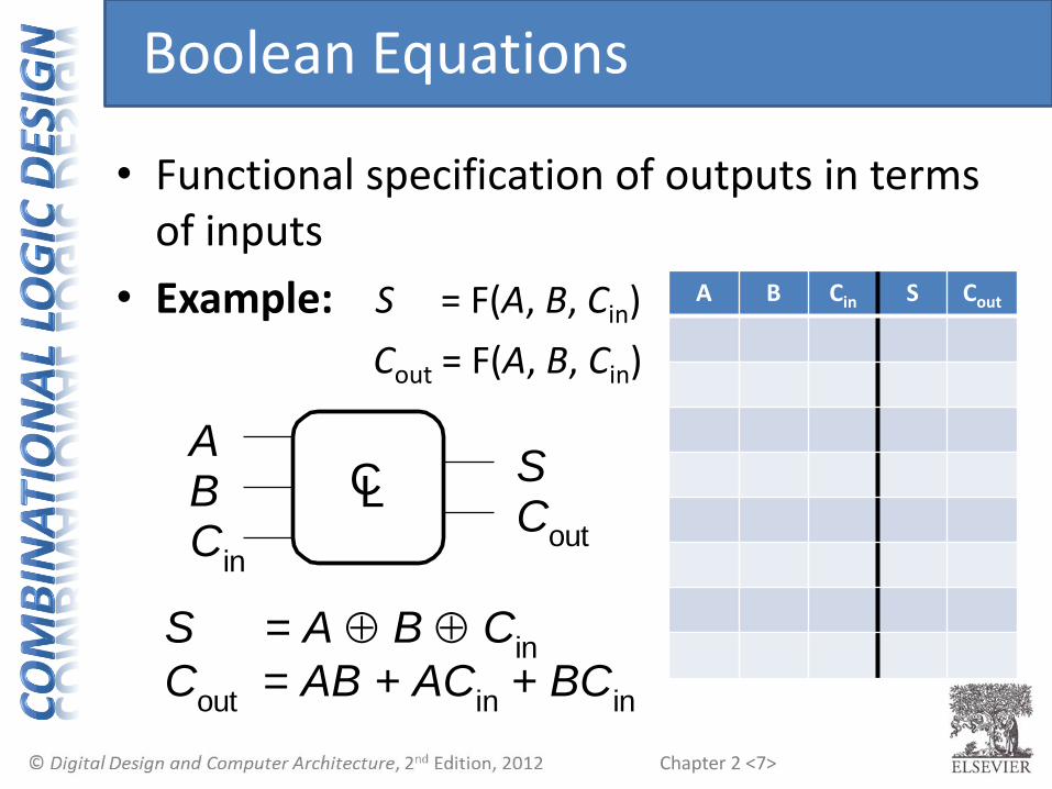
• Functional specification of outputs in terms of inputs
• Example: S = F(A, B, Cin)
Cout = F(A, B, Cin)
AS
S = A B Cin
Cout
= AB + ACin + BC
in
BC
in
CLC
out
Boolean Equations
A B Cin S Cout

Chapter 2 <8>
Goals:
• Systematically express logical functions using Boolean equations
• To simplify Boolean equations
Functional specification

Chapter 2 <9>
• Note: New homework instructions starting with HW03
• Homework is due at the beginning of class
• Homework must be organized, legible (messy is not), and stapled to be graded
Administrative Notes

Chapter 2 <10>
• Complement: variable with a bar over itA, B, C
• Literal: variable or its complementA, A, B, B, C, C
• Implicant: product of literalsABC, AC, BC
• Minterm: product that includes all input variablesABC, ABC, ABC
• Maxterm: sum that includes all input variables(A+B+C), (A+B+C), (A+B+C)
Some Definitions

Chapter 2 <11>
• All equations can be written in SOP form
• Each row has a minterm
• A minterm is a product (AND) of literals
• Each minterm is TRUE for that row (and only that row)
A B Y
0 0
0 1
1 0
1 1
0
1
0
1
minterm
A B
A B
A B
A B
minterm
name
m0
m1
m2
m3
Canonical Sum-of-Products (SOP) Form

Chapter 2 <12>
Y = F(A, B) =
• All equations can be written in SOP form
• Each row has a minterm
• A minterm is a product (AND) of literals
• Each minterm is TRUE for that row (and only that row)
• Form function by ORing minterms where the output is TRUE
A B Y
0 0
0 1
1 0
1 1
0
1
0
1
minterm
A B
A B
A B
A B
minterm
name
m0
m1
m2
m3
Canonical Sum-of-Products (SOP) Form
Chapter 2 <13>
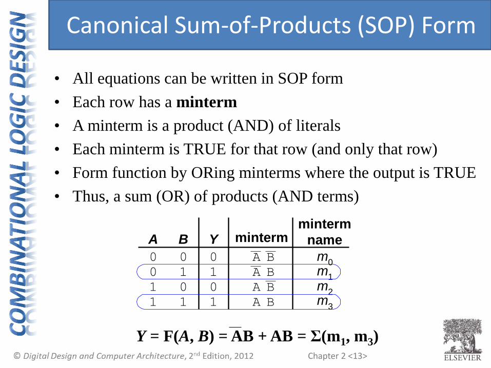
Y = F(A, B) = AB + AB = Σ(m1, m3)
Canonical Sum-of-Products (SOP) Form
• All equations can be written in SOP form
• Each row has a minterm
• A minterm is a product (AND) of literals
• Each minterm is TRUE for that row (and only that row)
• Form function by ORing minterms where the output is TRUE
• Thus, a sum (OR) of products (AND terms)
A B Y
0 0
0 1
1 0
1 1
0
1
0
1
minterm
A B
A B
A B
A B
minterm
name
m0
m1
m2
m3

Chapter 2 <14>
Y = F(A, B) =
SOP Example
• Steps:
• Find minterms that result in Y=1
• Sum “TRUE” minterms
A B Y
0 0 1
0 1 1
1 0 0
1 1 0

Chapter 2 <15>
Aside: Precedence
• AND has precedence over OR
• In other words:
• AND is performed before OR
• Example:
• 𝑌 = ҧ𝐴 ⋅ 𝐵 + 𝐴 ⋅ 𝐵
• Equivalent to:
• 𝑌 = ҧ𝐴𝐵 + (𝐴𝐵)

Chapter 2 <16>
• All Boolean equations can be written in POS form
• Each row has a maxterm
• A maxterm is a sum (OR) of literals
• Each maxterm is FALSE for that row (and only that row)
Canonical Product-of-Sums (POS) Form
A + B
A B Y
0 0
0 1
1 0
1 1
0
1
0
1
maxterm
A + B
A + B
A + B
maxterm
name
M0
M1
M2
M3
Chapter 2 <17>
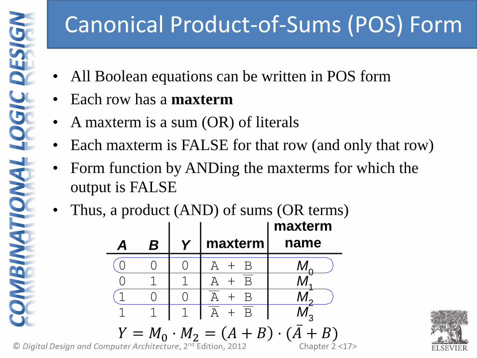
• All Boolean equations can be written in POS form
• Each row has a maxterm
• A maxterm is a sum (OR) of literals
• Each maxterm is FALSE for that row (and only that row)
• Form function by ANDing the maxterms for which the
output is FALSE
• Thus, a product (AND) of sums (OR terms)
Canonical Product-of-Sums (POS) Form
A + B
A B Y
0 0
0 1
1 0
1 1
0
1
0
1
maxterm
A + B
A + B
A + B
maxterm
name
M0
M1
M2
M3
𝑌 = 𝑀0 ⋅ 𝑀2 = 𝐴 + 𝐵 ⋅ ( ҧ𝐴 + 𝐵)

Chapter 2 <18>
• Sum of Products (SOP)
• Implement the “ones” of the output
• Sum all “one” terms OR results in “one”
• Product of Sums (POS)
• Implement the “zeros” of the output
• Multiply “zero” terms AND results in “zero”
SOP and POS Comparison

Chapter 2 <19>
• You are going to the cafeteria for lunch
– You will eat lunch (E=1)
– If it’s open (O=1) and
– If they’re not serving corndogs (C=0)
• Write a truth table for determining if you will eat lunch (E).
O C E
0 0
0 1
1 0
1 1
Boolean Equations Example

Chapter 2 <20>
• You are going to the cafeteria for lunch
– You will eat lunch (E=1)
– If it’s open (O=1) and
– If they’re not serving corndogs (C=0)
• Write a truth table for determining if you will eat lunch (E).
O C E
0 0
0 1
1 0
1 1
0
0
1
0
Boolean Equations Example

Chapter 2 <21>
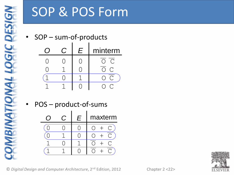
• SOP – sum-of-products
• POS – product-of-sums
O C E0 0
0 1
1 0
1 1
minterm
O C
O C
O C
O C
O + C
O C E
0 0
0 1
1 0
1 1
maxterm
O + C
O + C
O + C
SOP & POS Form
Chapter 2 <22>
• SOP – sum-of-products
• POS – product-of-sums
O + C
O C E
0 0
0 1
1 0
1 1
0
0
1
0
maxterm
O + C
O + C
O + C
O C E
0 0
0 1
1 0
1 1
0
0
1
0
minterm
O C
O C
O C
O C
SOP & POS Form

Chapter 2 <23>
• SOP – sum-of-products
• POS – product-of-sums
O + C
O C E
0 0
0 1
1 0
1 1
0
0
1
0
maxterm
O + C
O + C
O + C
O C E
0 0
0 1
1 0
1 1
0
0
1
0
minterm
O C
O C
O C
O CE = OC
= Σ(m2)
SOP & POS Form

Chapter 2 <24>
• SOP – sum-of-products
• POS – product-of-sums
O + C
O C E
0 0
0 1
1 0
1 1
0
0
1
0
maxterm
O + C
O + C
O + C
O C E
0 0
0 1
1 0
1 1
0
0
1
0
minterm
O C
O C
O C
O C
E = (O + C)(O + C)(O + C)
= Π(M0, M1, M3)
E = OC
= Σ(m2)
SOP & POS Form

Chapter 2 <25>
• Axioms and theorems to simplify Boolean equations
• Like regular algebra, but simpler: variables have only two values (1 or 0)
• Duality in axioms and theorems:– ANDs and ORs, 0’s and 1’s interchanged
Boolean Algebra

Chapter 2 <26>
Boolean Axioms

Chapter 2 <27>
Duality in Boolean axioms and theorems:– ANDs and ORs, 0’s and 1’s interchanged
Duality

Chapter 2 <28>
Boolean Axioms

Chapter 2 <29>
Boolean Axioms
Dual: Exchange:• and + 0 and 1

Chapter 2 <30>
Boolean Axioms
Dual: Exchange:• and + 0 and 1

Chapter 2 <31>
Basic Boolean Theorems
B = B

Chapter 2 <32>
Basic Boolean Theorems: Duals
Dual: Exchange:• and + 0 and 1

Chapter 2 <33>
• B 1 = B
• B + 0 = B
T1: Identity Theorem

Chapter 2 <34>
1 =
=
B
0B
B
B
• B 1 = B
• B + 0 = B
T1: Identity Theorem
Chapter 2 <35>
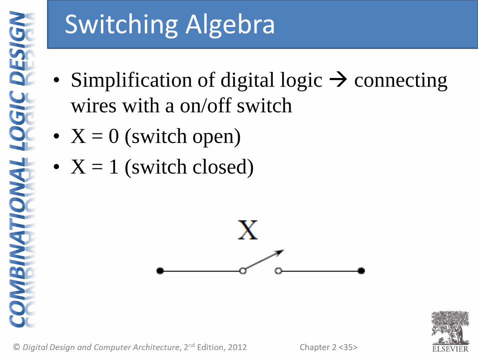
• Simplification of digital logic connecting
wires with a on/off switch
• X = 0 (switch open)
• X = 1 (switch closed)
Switching Algebra

Chapter 2 <36>
• Switching circuit in series performs AND
• 1 is connected to 2 iff A AND B are 1
Series Switching Network: AND

Chapter 2 <37>
• Switching circuit in parallel performs OR
• 1 is connected to 2 if A OR B is 1
Parallel Switching Network: OR

Chapter 2 <38>
1 =
=
B
0B
B
B
• B 1 = B
• B + 0 = B
T1: Identity Theorem

Chapter 2 <39>
• B 0 = 0
• B + 1 = 1
T2: Null Element Theorem

Chapter 2 <40>
0 =
=
B
1B
1
0
• B 0 = 0
• B + 1 = 1
T2: Null Element Theorem

Chapter 2 <41>
• B B = B
• B + B = B
T3: Idempotency Theorem

Chapter 2 <42>
B =
=
B
BB
B
B
• B B = B
• B + B = B
T3: Idempotency Theorem

Chapter 2 <43>
• B = B
T4: Involution Theorem

Chapter 2 <44>
= BB
• B = B
T4: Involution Theorem
0
1
1
0
0
1

Chapter 2 <45>
• B B = 0
• B + B = 1
T5: Complements Theorem

Chapter 2 <46>
B =
=
B
BB
1
0
• B B = 0
• B + B = 1
T5: Complements Theorem

Chapter 2 <47>
Recap: Basic Boolean Theorems

Chapter 2 <48>
Boolean Theorems of Several Vars
Number Theorem Name
T6 B•C = C•B Commutativity
T7 (B•C) • D = B • (C • D) Associativity
T8 B • (C + D) = (B•C) + (B•D) Distributivity
T9 B• (B+C) = B Covering
T10 (B•C) + (B•C) = B Combining
T11 B•C + (B•D) + (C•D) =B•C + B•D
Consensus

Chapter 2 <49>
Boolean Theorems of Several Vars
Number Theorem Name
T6 B•C = C•B Commutativity
T7 (B•C) • D = B • (C • D) Associativity
T8 B • (C + D) = (B•C) + (B•D) Distributivity
T9 B• (B+C) = B Covering
T10 (B•C) + (B•C) = B Combining
T11 B•C + (B•D) + (C•D) =B•C + B•D
Consensus
How do we prove these are true?

Chapter 2 <50>
How to Prove Boolean Relation
• Method 1: Perfect induction
• Method 2: Use other theorems and axioms
to simplify the equation
• Make one side of the equation look like
the other

Chapter 2 <51>
Proof by Perfect Induction
• Also called: proof by exhaustion
• Check every possible input value
• If two expressions produce the same value
for every possible input combination, the
expressions are equal

Chapter 2 <52>
Example: Proof by Perfect Induction
Number Theorem Name
T6 B•C = C•B Commutativity
0 00 11 01 1
B C BC CB

Chapter 2 <53>
Example: Proof by Perfect Induction
Number Theorem Name
T6 B•C = C•B Commutativity
0 00 11 01 1
B C BC CB
0 00 00 01 1

Chapter 2 <54>
Boolean Theorems of Several Vars
Number Theorem Name
T6 B•C = C•B Commutativity
T7 (B•C) • D = B • (C • D) Associativity
T8 B • (C + D) = (B•C) + (B•D) Distributivity
T9 B• (B+C) = B Covering
T10 (B•C) + (B•C) = B Combining
T11 B•C + (B•D) + (C•D) =B•C + B•D
Consensus

Chapter 2 <55>
T7: Associativity
Number Theorem Name
T7 (B•C) • D = B • (C • D) Associativity

Chapter 2 <56>
T8: Distributivity
Number Theorem Name
T8 B • (C + D) = (B•C) + (B•D) Distributivity

Chapter 2 <57>
T9: Covering
Number Theorem Name
T9 B• (B+C) = B Covering

Chapter 2 <58>
T9: Covering
Number Theorem Name
T9 B• (B+C) = B Covering
Prove true by:
• Method 1: Perfect induction
• Method 2: Using other theorems and axioms

Chapter 2 <59>
T9: Covering
Number Theorem Name
T9 B• (B+C) = B Covering
0 00 11 01 1
B C (B+C) B(B+C)
Method 1: Perfect Induction

Chapter 2 <60>
T9: Covering
Number Theorem Name
T9 B• (B+C) = B Covering
Method 1: Perfect Induction
0 00 11 01 1
B C (B+C) B(B+C)
0 01 01 11 1

Chapter 2 <61>
T9: Covering
Number Theorem Name
T9 B• (B+C) = B Covering
Method 2: Prove true using other axioms and
theorems.

Chapter 2 <62>
T9: Covering
Number Theorem Name
T9 B• (B+C) = B Covering
Method 2: Prove true using other axioms and
theorems.
B•(B+C) = B•B + B•C T8: Distributivity
= B + B•C T3: Idempotency
= B•(1 + C) T8: Distributivity
= B•(1) T2: Null element
= B T1: Identity

Chapter 2 <63>
T10: Combining
Number Theorem Name
T10 (B•C) + (B•C) = B Combining
Prove true using other axioms and theorems:

Chapter 2 <64>
T10: Combining
Number Theorem Name
T10 (B•C) + (B•C) = B Combining
Prove true using other axioms and theorems:
B•C + B•C = B•(C+C) T8: Distributivity
= B•(1) T5’: Complements
= B T1: Identity

Chapter 2 <65>
T11: Consensus
Number Theorem Name
T11 (B•C) + (B•D) + (C•D) =(B•C) + B•D
Consensus
Prove true using (1) perfect induction or (2) other axioms and
theorems.

Chapter 2 <66>
Recap: Boolean Thms of Several Vars
Number Theorem Name
T6 B•C = C•B Commutativity
T7 (B•C) • D = B • (C • D) Associativity
T8 B • (C + D) = (B•C) + (B•D) Distributivity
T9 B• (B+C) = B Covering
T10 (B•C) + (B•C) = B Combining
T11 B•C + (B•D) + (C•D) =B•C + B•D
Consensus

Chapter 2 <67>
Boolean Thms of Several Vars: Duals
# Theorem Dual Name
T6 B•C = C•B B+C = C+B Commutativity
T7 (B•C) • D = B • (C•D) (B + C) + D = B + (C + D) Associativity
T8 B • (C + D) = (B•C) + (B•D) B + (C•D) = (B+C) (B+D) Distributivity
T9 B • (B+C) = B B + (B•C) = B Covering
T10 (B•C) + (B•C) = B (B+C) • (B+C) = B Combining
T11 (B•C) + (B•D) + (C•D) =(B•C) + (B•D)
(B+C) • (B+D) • (C+D) =(B+C) • (B+D)
Consensus
Dual: Replace: • with + 0 with 1

Chapter 2 <68>
Boolean Thms of Several Vars: Duals
# Theorem Dual Name
T6 B•C = C•B B+C = C+B Commutativity
T7 (B•C) • D = B • (C•D) (B + C) + D = B + (C + D) Associativity
T8 B • (C + D) = (B•C) + (B•D) B + (C•D) = (B+C) (B+D) Distributivity
T9 B • (B+C) = B B + (B•C) = B Covering
T10 (B•C) + (B•C) = B (B+C) • (B+C) = B Combining
T11 (B•C) + (B•D) + (C•D) =(B•C) + (B•D)
(B+C) • (B+D) • (C+D) =(B+C) • (B+D)
Consensus
Dual: Replace: • with + 0 with 1
Warning: T8’ differs from traditional algebra: OR (+) distributes over AND (•)

Chapter 2 <69>
Boolean Thms of Several Vars: Duals
# Theorem Dual Name
T6 B•C = C•B B+C = C+B Commutativity
T7 (B•C) • D = B • (C•D) (B + C) + D = B + (C + D) Associativity
T8 B • (C + D) = (B•C) + (B•D) B + (C•D) = (B+C) (B+D) Distributivity
T9 B • (B+C) = B B + (B•C) = B Covering
T10 (B•C) + (B•C) = B (B+C) • (B+C) = B Combining
T11 (B•C) + (B•D) + (C•D) =(B•C) + (B•D)
(B+C) • (B+D) • (C+D) =(B+C) • (B+D)
Consensus
Axioms and theorems are useful for simplifying equations.

Chapter 2 <70>
Simplifying an Equation
• Reducing an equation to the fewest
number of implicants, where each
implicant has the fewest literals

Chapter 2 <71>
Simplifying an Equation
• Reducing an equation to the fewest
number of implicants, where each
implicant has the fewest literals
Recall: Implicant: product of literals
ABC, AC, BC Literal: variable or its complement
A, A, B, B, C, C

Chapter 2 <72>
Simplifying an Equation
• Reducing an equation to the fewest
number of implicants, where each
implicant has the fewest literals
Recall: Implicant: product of literals
ABC, AC, BC Literal: variable or its complement
A, A, B, B, C, C
• Also called: minimizing the equation

Chapter 2 <73>
Simplification methods• Distributivity (T8, T8’)
B (C+D) = BC + BD
B + CD = (B+ C)(B+D)
• Covering (T9’)
A + AP = A
• Combining (T10)
PA + PA = P

Chapter 2 <74>
Simplification methods• Distributivity (T8, T8’)
B (C+D) = BC + BD
B + CD = (B+ C)(B+D)
• Covering (T9’)
A + AP = A
• Combining (T10)
PA + PA = P
• Expansion
P = PA + PA
A = A + AP
• Duplication
A = A + A

Chapter 2 <75>
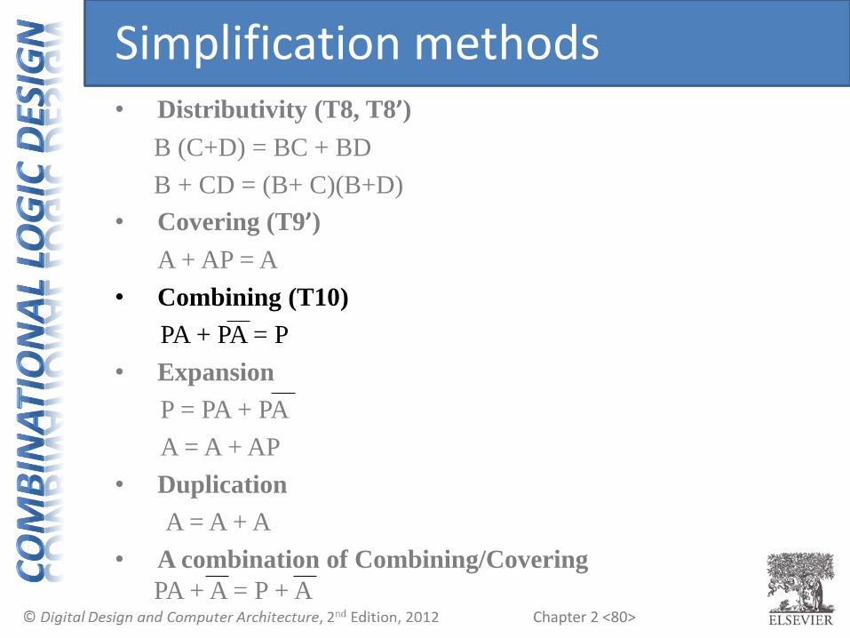
Simplification methods• Distributivity (T8, T8’)
B (C+D) = BC + BD
B + CD = (B+ C)(B+D)
• Covering (T9’)
A + AP = A
• Combining (T10)
PA + PA = P
• Expansion
P = PA + PA
A = A + AP
• Duplication
A = A + A
• A combination of Combining/Covering
PA + A = P + A

Chapter 2 <76>
Simplification methods
• A combination of Combining/Covering
PA + A = P + A
Proof: PA + A = PA + (A + AP) T9’ Covering
= PA + PA + A T6 Commutativity
= P(A + A) + A T8 Distributivity
= P(1) + A T5’ Complements
= P + A T1 Identity

Chapter 2 <77>
T11: Consensus
Number Theorem Name
T11 (B•C) + (B•D) + (C•D) =(B•C) + B•D
Consensus
Prove using other theorems and axioms:

Chapter 2 <78>
T11: Consensus
Number Theorem Name
T11 (B•C) + (B•D) + (C•D) =(B•C) + B•D
Consensus
Prove using other theorems and axioms:
B•C + B•D + C•D
= BC + BD + (CDB+CDB) T10: Combining
= BC + BD + BCD+BCD T6: Commutativity
= BC + BCD + BD + BCD T6: Commutativity
= (BC + BCD) + (BD + BCD) T7: Associativity
= BC + BD T9’: Covering

Chapter 2 <79>
Recap: Boolean Thms of Several Vars
# Theorem Dual Name
T6 B•C = C•B B+C = C+B Commutativity
T7 (B•C) • D = B • (C•D) (B + C) + D = B + (C + D) Associativity
T8 B • (C + D) = (B•C) + (B•D) B + (C•D) = (B+C) (B+D) Distributivity
T9 B • (B+C) = B B + (B•C) = B Covering
T10 (B•C) + (B•C) = B (B+C) • (B+C) = B Combining
T11 (B•C) + (B•D) + (C•D) =(B•C) + (B•D)
(B+C) • (B+D) • (C+D) =(B+C) • (B+D)
Consensus
Chapter 2 <80>
Simplification methods• Distributivity (T8, T8’)
B (C+D) = BC + BD
B + CD = (B+ C)(B+D)
• Covering (T9’)
A + AP = A
• Combining (T10)
PA + PA = P
• Expansion
P = PA + PA
A = A + AP
• Duplication
A = A + A
• A combination of Combining/Covering
PA + A = P + A

Chapter 2 <81>
Y = AB + AB
Simplifying Boolean Equations
Example 1:

Chapter 2 <82>
Y = AB + AB
Y = A T10: Combining
or
= A(B + B) T8: Distributivity
= A(1) T5’: Complements
= A T1: Identity
Simplifying Boolean Equations
Example 1:

Chapter 2 <83>
Simplification methods• Distributivity (T8, T8’)
B (C+D) = BC + BD
B + CD = (B+ C)(B+D)
• Covering (T9’)
A + AP = A
• Combining (T10)
PA + PA = P
• Expansion
P = PA + PA
A = A + AP
• Duplication
A = A + A
• A combination of Combining/Covering
PA + A = P + A

Chapter 2 <84>
Y = A(AB + ABC)
Example 2:
Simplifying Boolean Equations

Chapter 2 <85>
Y = A(AB + ABC)
= A(AB(1 + C)) T8: Distributivity
= A(AB(1)) T2’: Null Element
= A(AB) T1: Identity
= (AA)B T7: Associativity
= AB T3: Idempotency
Example 2:
Simplifying Boolean Equations

Chapter 2 <86>
Simplification methods• Distributivity (T8, T8’)
B (C+D) = BC + BD
B + CD = (B+ C)(B+D)
• Covering (T9’)
A + AP = A
• Combining (T10)
PA + PA = P
• Expansion
P = PA + PA
A = A + AP
• Duplication
A = A + A
• A combination of Combining/Covering
PA + A = P + A

Chapter 2 <87>
Y = A’BC + A’ Recall: A’ = A
Example 3:
Simplifying Boolean Equations

Chapter 2 <88>
Y = A’BC + A’ Recall: A’ = A
= A’ T9’ Covering: X + XY = X
or
= A’(BC + 1) T8: Distributivity
= A’(1) T2’: Null Element
= A’ T1: Identity
Example 3:
Simplifying Boolean Equations

Chapter 2 <89>
Simplification methods• Distributivity (T8, T8’)
B (C+D) = BC + BD
B + CD = (B+ C)(B+D)
• Covering (T9’)
A + AP = A
• Combining (T10)
PA + PA = P
• Expansion
P = PA + PA
A = A + AP
• Duplication
A = A + A
• A combination of Combining/Covering
PA + A = P + A
Chapter 2 <90>
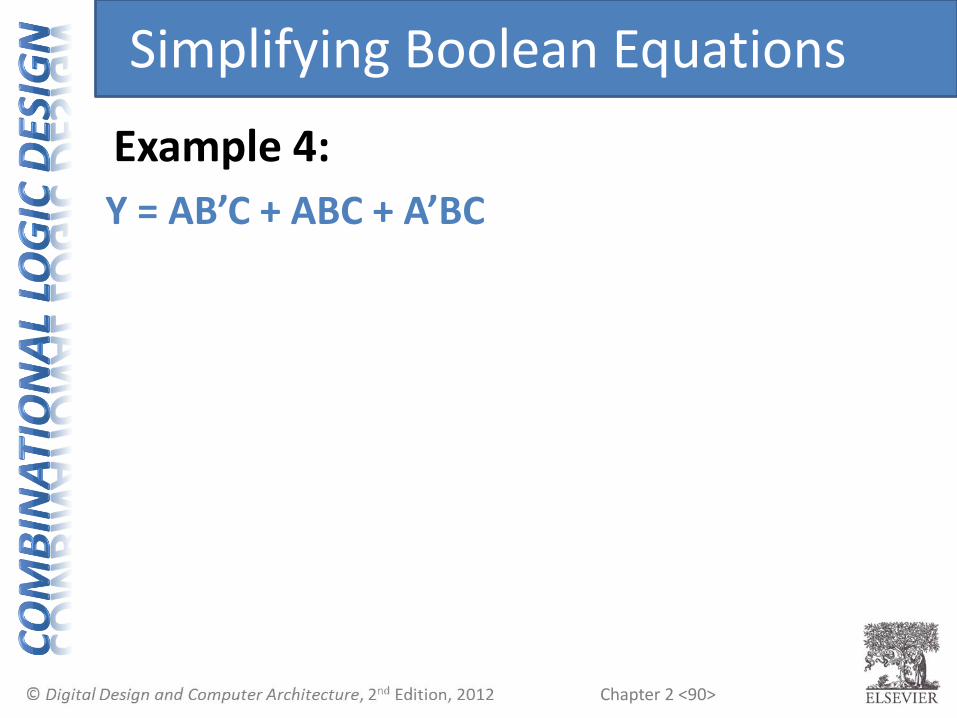
Y = AB’C + ABC + A’BC
Example 4:
Simplifying Boolean Equations

Chapter 2 <91>
Y = AB’C + ABC + A’BC
= AB’C + ABC + ABC + A’BC T3’: Idempotency
= (AB’C+ABC) + (ABC+A’BC) T7’: Associativity
= AC + BC T10: Combining
Example 4:
Simplifying Boolean Equations

Chapter 2 <92>
Simplification methods• Distributivity (T8, T8’)
B (C+D) = BC + BD
B + CD = (B+ C)(B+D)
• Covering (T9’)
A + AP = A
• Combining (T10)
PA + PA = P
• Expansion
P = PA + PA
A = A + AP
• Duplication
A = A + A
• A combination of Combining/Covering
PA + A = P + A

Chapter 2 <93>
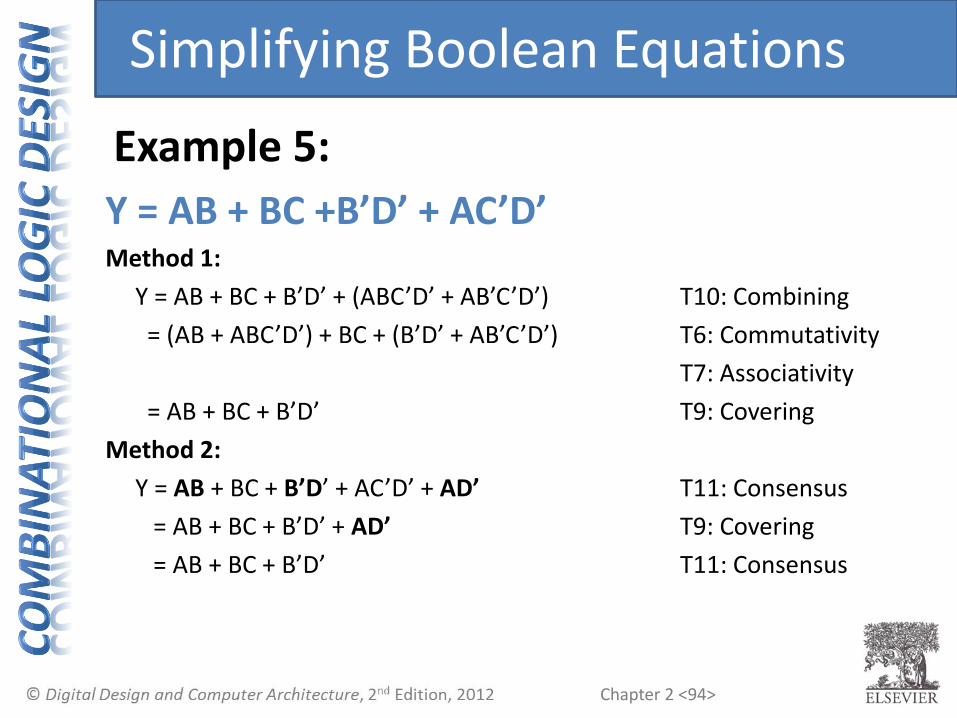
Y = AB + BC +B’D’ + AC’D’
Example 5:
Simplifying Boolean Equations
Chapter 2 <94>
Y = AB + BC +B’D’ + AC’D’Method 1:
Y = AB + BC + B’D’ + (ABC’D’ + AB’C’D’) T10: Combining
= (AB + ABC’D’) + BC + (B’D’ + AB’C’D’) T6: Commutativity
T7: Associativity
= AB + BC + B’D’ T9: Covering
Method 2:
Y = AB + BC + B’D’ + AC’D’ + AD’ T11: Consensus
= AB + BC + B’D’ + AD’ T9: Covering
= AB + BC + B’D’ T11: Consensus
Example 5:
Simplifying Boolean Equations

Chapter 2 <95>
Simplification methods• Distributivity (T8, T8’)
B (C+D) = BC + BD
B + CD = (B+ C)(B+D)
• Covering (T9’)
A + AP = A
• Combining (T10)
PA + PA = P
• Expansion
P = PA + PA
A = A + AP
• Duplication
A = A + A
• A combination of Combining/Covering
PA + A = P + A
Chapter 2 <96>
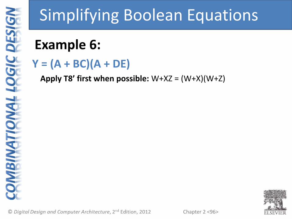
Y = (A + BC)(A + DE)Apply T8’ first when possible: W+XZ = (W+X)(W+Z)
Example 6:
Simplifying Boolean Equations

Chapter 2 <97>
Y = (A + BC)(A + DE)Apply T8’ first when possible: W+XZ = (W+X)(W+Z)
Make: X = BC, Z = DE and rewrite equation
Y = (A+X)(A+Z) substitution (X=BC, Z=DE)
= A + XZ T8’: Distributivity
= A + BCDE substitution
or
Y = AA + ADE + ABC + BCDE T8: Distributivity
= A + ADE + ABC + BCDE T3: Idempotency
= A + ADE + ABC + BCDE
= A + ABC + BCDE T9’: Covering
= A + BCDE T9’: Covering
Example 6:
Simplifying Boolean Equations

Chapter 2 <98>
Y = (A + BC)(A + DE)Apply T8’ first when possible: W+XZ = (W+X)(W+Z)
Make: X = BC, Z = DE and rewrite equation
Y = (A+X)(A+Z) substitution (X=BC, Z=DE)
= A + XZ T8’: Distributivity
= A + BCDE substitution
or
Y = AA + ADE + ABC + BCDE T8: Distributivity
= A + ADE + ABC + BCDE T3: Idempotency
= A + ADE + ABC + BCDE
= A + ABC + BCDE T9’: Covering
= A + BCDE T9’: Covering
Example 6:
Simplifying Boolean Equations
This is calledmultiplying outan expression to getsum-of-products (SOP) form.

Chapter 2 <99>
Midterm 1: Thursday, Oct. 5th
• In class: 1 hour and 15 minutes
• Chap 1 – 2.6
• Closed book, closed notes
• No calculator
• Boolean Theorems & Axioms document will be attached as last page of the exam for your convenience
Reminder

Chapter 2 <100>
An expression is in simplified sum-of-products (SOP) form when all products contain literals only.• SOP form: Y = AB + BC’ + DE• NOT SOP form: Y = DF + E(A’+B)• SOP form: Z = A + BC + DE’F
Multiplying Out: SOP Form

Chapter 2 <101>
Y = (A + C + D + E)(A + B)Apply T8’ first when possible: W+XZ = (W+X)(W+Z)
Example:
Multiplying Out: SOP Form

Chapter 2 <102>
Y = (A + C + D + E)(A + B)Apply T8’ first when possible: W+XZ = (W+X)(W+Z)
Make: X = (C+D+E), Z = B and rewrite equation
Y = (A+X)(A+Z) substitution (X=(C+D+E), Z=B)
= A + XZ T8’: Distributivity
= A + (C+D+E)B substitution
= A + BC + BD + BE T8: Distributivity
or
Y = AA+AB+AC+BC+AD+BD+AE+BE T8: Distributivity
= A+AB+AC+AD+AE+BC+BD+BE T3: Idempotency
= A + BC + BD + BE T9’: Covering
Example:
Multiplying Out: SOP Form

Chapter 2 <103>
• SOP – sum-of-products
• POS – product-of-sums
O + C
O C E
0 0
0 1
1 0
1 1
0
0
1
0
maxterm
O + C
O + C
O + C
O C E
0 0
0 1
1 0
1 1
0
0
1
0
minterm
O C
O C
O C
O C
E = (O + C)(O + C)(O + C)
= Π(M0, M1, M3)
E = OC
= Σ(m2)
Canonical SOP & POS Form

Chapter 2 <104>
An expression is in simplified product-of-sums (POS) form when all sums contain literals only.• POS form: Y = (A+B)(C+D)(E’+F)• NOT POS form: Y = (D+E)(F’+GH)• POS form: Z = A(B+C)(D+E’)
Factoring: POS Form

Chapter 2 <105>
Y = (A + B’CDE)Apply T8’ first when possible: W+XZ = (W+X)(W+Z)
Example 1:
Factoring: POS Form

Chapter 2 <106>
Y = (A + B’CDE)Apply T8’ first when possible: W+XZ = (W+X)(W+Z)
Make: X = B’C, Z = DE and rewrite equation
Y = (A+XZ) substitution (X=B’C, Z=DE)
= (A+B’C)(A+DE) T8’: Distributivity
= (A+B’)(A+C)(A+D)(A+E) T8’: Distributivity
Example 1:
Factoring: POS Form

Chapter 2 <107>
Y = AB + C’DE + FApply T8’ first when possible: W+XZ = (W+X)(W+Z)
Example 2:
Factoring: POS Form

Chapter 2 <108>
Y = AB + C’DE + FApply T8’ first when possible: W+XZ = (W+X)(W+Z)
Make: W = AB, X = C’, Z = DE and rewrite equation
Y = (W+XZ) + F substitution W = AB, X = C’, Z = DE
= (W+X)(W+Z) + F T8’: Distributivity
= (AB+C’)(AB+DE)+F substitution
= (A+C’)(B+C’)(AB+D)(AB+E)+F T8’: Distributivity
= (A+C’)(B+C’)(A+D)(B+D)(A+E)(B+E)+F T8’: Distributivity
= (A+C’+F)(B+C’+F)(A+D+F)(B+D+F)(A+E+F)(B+E+F) T8’: Distributivity
Example 2:
Factoring: POS Form

Chapter 2 <109>
Boolean Thms of Several Vars: Duals
# Theorem Dual Name
T6 B•C = C•B B+C = C+B Commutativity
T7 (B•C) • D = B • (C•D) (B + C) + D = B + (C + D) Associativity
T8 B • (C + D) = (B•C) + (B•D) B + (C•D) = (B+C) (B+D) Distributivity
T9 B • (B+C) = B B + (B•C) = B Covering
T10 (B•C) + (B•C) = B (B+C) • (B+C) = B Combining
T11 (B•C) + (B•D) + (C•D) =(B•C) + (B•D)
(B+C) • (B+D) • (C+D) =(B+C) • (B+D)
Consensus
Axioms and theorems are useful for simplifying equations.

Chapter 2 <110>
Simplification methods• Distributivity (T8, T8’)
B (C+D) = BC + BD
B + CD = (B+ C)(B+D)
• Covering (T9’)
A + AP = A
• Combining (T10)
PA + PA = P
• Expansion
P = PA + PA
A = A + AP
• Duplication
A = A + A
• A combination of Combining/Covering
PA + A = P + A
Chapter 2 <111>
DeMorgan’s Theorem
Number Theorem Name
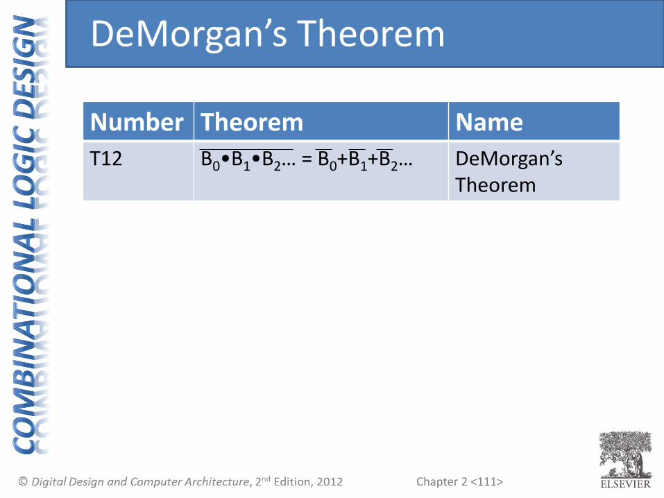
T12 B0•B1•B2… = B0+B1+B2… DeMorgan’sTheorem
Chapter 2 <112>
DeMorgan’s Theorem
Number Theorem Name
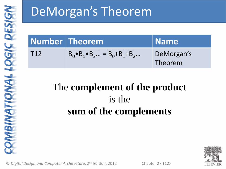
T12 B0•B1•B2… = B0+B1+B2… DeMorgan’sTheorem
The complement of the product
is the
sum of the complements

Chapter 2 <113>
# Theorem Dual Name
T12 B0•B1•B2… = B0+B1+B2…
B0+B1+B2… = B0•B1•B2…
DeMorgan’sTheorem
DeMorgan’s Theorem: Dual

Chapter 2 <114>
# Theorem Dual Name
T12 B0•B1•B2… = B0+B1+B2…
B0+B1+B2… = B0•B1•B2…
DeMorgan’sTheorem
DeMorgan’s Theorem: Dual
The complement of the product
is the
sum of the complements
Chapter 2 <115>
DeMorgan’s Theorem: Dual
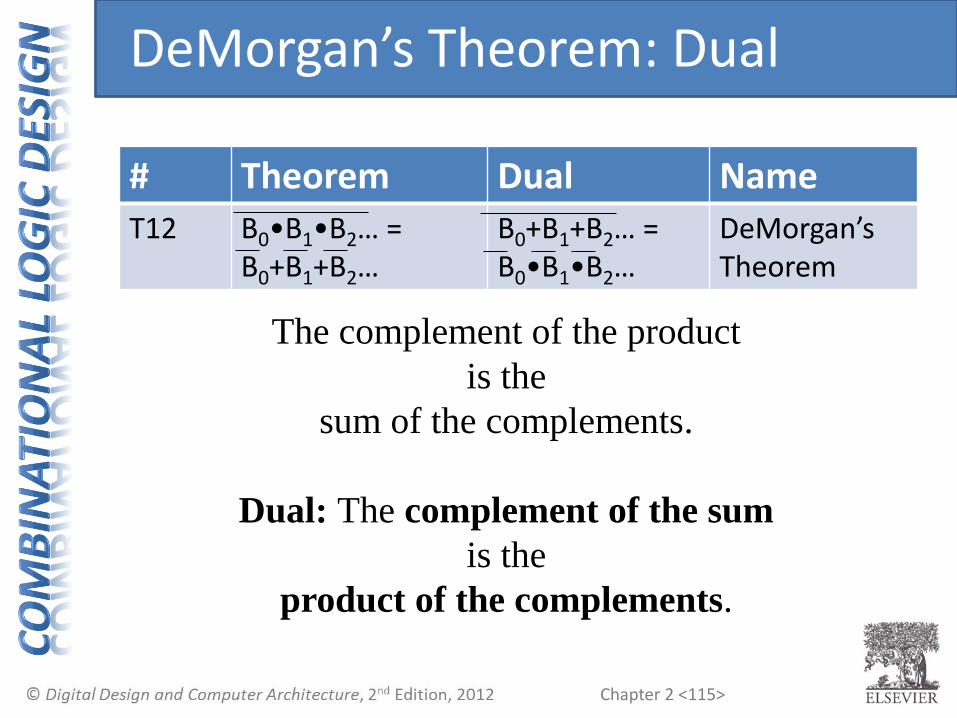
# Theorem Dual Name
T12 B0•B1•B2… = B0+B1+B2…
B0+B1+B2… = B0•B1•B2…
DeMorgan’sTheorem
The complement of the product
is the
sum of the complements.
Dual: The complement of the sum
is the
product of the complements.

Chapter 2 <116>
• Y = AB = A + B
• Y = A + B = A B
AB
Y
AB
Y
AB
Y
AB
Y
DeMorgan’s Theorem

Chapter 2 <117>
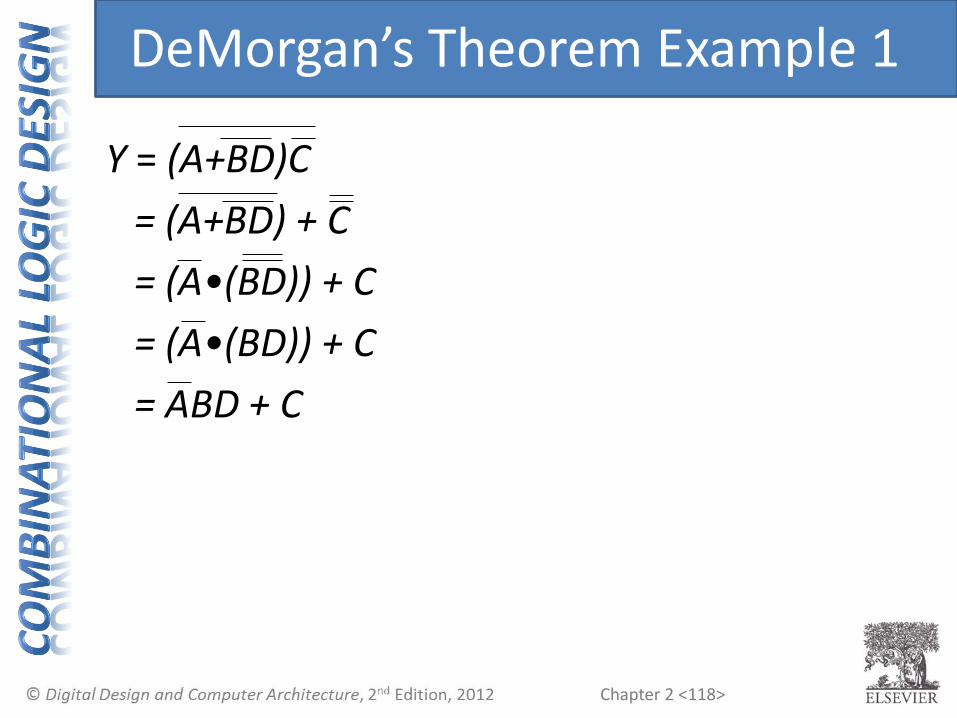
Y = (A+BD)C
DeMorgan’s Theorem Example 1
Chapter 2 <118>
Y = (A+BD)C
= (A+BD) + C
= (A•(BD)) + C
= (A•(BD)) + C
= ABD + C
DeMorgan’s Theorem Example 1

Chapter 2 <119>
Y = (ACE+D) + B
DeMorgan’s Theorem Example 2

Chapter 2 <120>
Y = (ACE+D) + B
= (ACE+D) • B
= (ACE•D) • B
= ((AC+E)•D) • B
= ((AC+E)•D) • B
= (ACD + DE) • B
= ABCD + BDE
DeMorgan’s Theorem Example 2

Chapter 2 <121>
• Backward:– Body changes
– Adds bubbles to inputs
• Forward:– Body changes
– Adds bubble to output
AB
YAB
Y
AB
YAB
Y
Bubble Pushing

Chapter 2 <122>
AB
YCD
• What is the Boolean expression for this
circuit?
Bubble Pushing

Chapter 2 <123>
AB
YCD
• What is the Boolean expression for this
circuit?
Y = AB + CD
Bubble Pushing

Chapter 2 <124>
AB
C
D
Y
• Begin at output, then work toward inputs
• Push bubbles on final output back
• Draw gates in a form so bubbles cancel
Bubble Pushing Rules
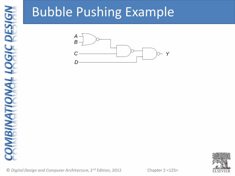
Chapter 2 <125>
AB
C Y
D
Bubble Pushing Example

Chapter 2 <126>
AB
C Y
D
no output
bubble
Bubble Pushing Example
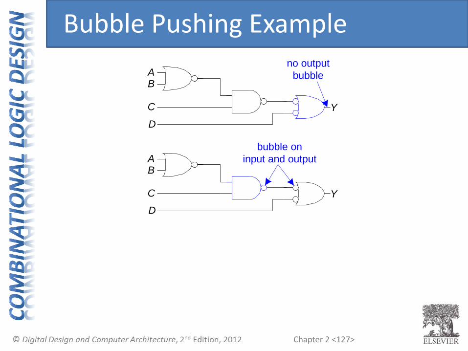
Chapter 2 <127>
bubble on
input and outputAB
C
D
Y
AB
C Y
D
no output
bubble
Bubble Pushing Example

Chapter 2 <128>
AB
C
D
Y
bubble on
input and outputAB
C
D
Y
AB
C Y
D
Y = ABC + D
no output
bubble
no bubble on
input and output
Bubble Pushing Example

Chapter 2 <129>
• SOP – sum-of-products
• POS – product-of-sums
O + C
O C E
0 0
0 1
1 0
1 1
0
0
1
0
maxterm
O + C
O + C
O + C
O C E
0 0
0 1
1 0
1 1
0
0
1
0
minterm
O C
O C
O C
O C
E = (O + C)(O + C)(O + C)
= Π(M0, M1, M3)
E = OC
= Σ(m2)
Canonical SOP & POS Form Revisited
How do we implement this logic function with gates?

Chapter 2 <130>
• Two-level logic: ANDs followed by ORs
• Example: Y = ABC + ABC + ABC
BA C
Y
minterm: ABC
minterm: ABC
minterm: ABC
A B C
From Logic to Gates

Chapter 2 <131>
• Inputs on the left (or top)
• Outputs on right (or bottom)
• Gates flow from left to right
• Straight wires are best
Circuit Schematics Rules
𝑌 = ത𝐵 ҧ𝐶 + 𝐴 ത𝐵

Chapter 2 <132>
• Wires always connect at a T junction
• A dot where wires cross indicates a connection between the wires
• Wires crossing without a dot make no connection
wires connect
at a T junction
wires connect
at a dot
wires crossing
without a dot do
not connect
Circuit Schematic Rules (cont.)

Chapter 2 <133>
A1
A0
0 00 11 01 1
Y3Y2
Y1
Y0A
3A2
0 00 00 00 0
0 00 10 11 01 10 0
0 10 10 11 0
0 11 01 01 10 00 1
1 01 01 11 1
1 01 11 11 1
A0
A1
PRIORITY
CiIRCUIT
A2
A3
Y0
Y1
Y2
Y3
• Example: Priority Circuit
Output asserted
corresponding to
most significant
TRUE input
Multiple-Output Circuits

Chapter 2 <134>
0
A1
A0
0 00 11 01 1
0
00
Y3Y2
Y1
Y0
0000
0011
0100
A3
A2
0 00 00 00 0
0 0 0 1 0 00 10 11 01 10 0
0 10 10 11 0
0 11 01 01 10 00 1
1 01 01 11 1
1 01 11 11 1
0001
1110
0000
0000
1 0 0 01111
0000
0000
0000
1 0 0 01 0 0 0
A0
A1
PRIORITY
CiIRCUIT
A2
A3
Y0
Y1
Y2
Y3
• Example: Priority Circuit
Output asserted
corresponding to
most significant
TRUE input
Multiple-Output Circuits

Chapter 2 <135>
A1
A0
0 00 11 01 1
0000
Y3Y2
Y1
Y0
0000
0011
0100
A3
A2
0 00 00 00 0
0 0 0 1 0 00 10 11 01 10 0
0 10 10 11 0
0 11 01 01 10 00 1
1 01 01 11 1
1 01 11 11 1
0001
1110
0000
0000
1 0 0 01111
0000
0000
0000
1 0 0 01 0 0 0
A3A
2A
1A
0
Y3
Y2
Y1
Y0
Priority Circuit Hardware

Chapter 2 <136>
A1
A0
0 00 11 01 1
0000
Y3Y2
Y1
Y0
0000
0011
0100
A3
A2
0 00 00 00 0
0 0 0 1 0 00 10 11 01 10 0
0 10 10 11 0
0 11 01 01 10 00 1
1 01 01 11 1
1 01 11 11 1
0001
1110
0000
0000
1 0 0 01111
0000
0000
0000
1 0 0 01 0 0 0
A1
A0
0 00 11 XX X
0000
Y3Y2
Y1
Y0
0001
0010
0100
A3
A2
0 00 00 00 1
X X 1 0 0 01 X
Don’t Cares
A3A
2A
1A
0
Y3
Y2
Y1
Y0
• Simplify truth table by ignoring entries
Much easier to read off Boolean equations
= 𝐴3
= 𝐴3𝐴2
= 𝐴3 𝐴2 𝐴1
= 𝐴3 𝐴2 𝐴1 𝐴0

Chapter 2 <137>
• Contention: circuit tries to drive output to 1 and 0– Actual value somewhere in between
– Could be 0, 1, or in forbidden zone
– Might change with voltage, temperature, time, noise
– Often causes excessive power dissipation
• Warnings: – Contention usually indicates a bug.
– X is used for “don’t care” and contention - look at the context to tell them apart
A = 1
Y = X
B = 0
Contention: X

Chapter 2 <138>
• Floating, high impedance, open, high Z
• Floating output might be 0, 1, or somewhere in between– A voltmeter won’t indicate whether a node is floating
Tristate Buffer
E A Y0 0 Z
0 1 Z
1 0 0
1 1 1
A
E
Y
Floating: Z
Note: tristate buffer has an enable bit (𝐸) to turn on the gate

Chapter 2 <139>
• Floating nodes are used in tristatebusses– Many different drivers
– Exactly one is active at
once
en1
to bus
from bus
en2
to bus
from bus
en3
to bus
from bus
en4
to bus
from bus
sh
are
d b
us
processor
video
Ethernet
memory
Tristate Busses

Chapter 2 <140>
• Boolean expressions can be minimized by combining terms
• PA + PA = P
• K-maps minimize equations graphically
• Put terms to combine close to one another
C00 01
0
1
Y
11 10AB
1
1
0
0
0
0
0
0
C 00 01
0
1
Y
11 10AB
ABC
ABC
ABC
ABC
ABC
ABC
ABC
ABC
B C0 0
0 1
1 0
1 1
A0
0
0
0
0 0
0 1
1 0
1 1
1
1
1
1
1
1
0
0
0
0
0
0
Y
Karnaugh Maps (K-Maps)
𝑌 = ҧ𝐴 ത𝐵 ҧ𝐶 + ҧ𝐴 ത𝐵𝐶 = ҧ𝐴 ത𝐵(𝐶 + ҧ𝐶)

Chapter 2 <141>
C00 01
0
1
Y
11 10AB
1
0
0
0
0
0
0
1
B C0 0
0 1
1 0
1 1
A0
0
0
0
0 0
0 1
1 0
1 1
1
1
1
1
1
1
0
0
0
0
0
0
Y
• Circle 1’s in adjacent squares
• In Boolean expression, include only
literals whose true and complement form
are not in the circle
𝑌 = ҧ𝐴 ത𝐵
K-Map
𝐶 not included because both 𝐶 and ҧ𝐶 included in circle

Chapter 2 <142>
C 00 01
0
1
Y
11 10AB
ABC
ABC
ABC
ABC
ABC
ABC
ABC
ABC
1
B C Y0 0 0
0 1 0
1 0
1 1 1
Truth Table
C 00 01
0
1
Y
11 10ABA
0
0
0
0
0 0 0
0 1 0
1 0 0
1 1 1
1
1
1
1
K-Map
3-Input K-Map

Chapter 2 <143>
• Complement: variable with a bar over it
A, B, C
• Literal: variable or its complement
A, A, B, B, C, C
• Implicant: product of literals
ABC, AC, BC
• Prime implicant: implicant corresponding to the largest circle in a K-map
K-Map Definitions
Chapter 2 <144>
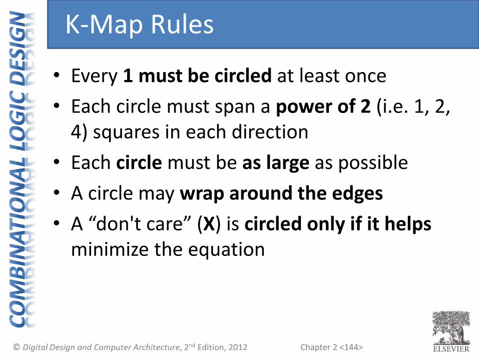
• Every 1 must be circled at least once
• Each circle must span a power of 2 (i.e. 1, 2, 4) squares in each direction
• Each circle must be as large as possible
• A circle may wrap around the edges
• A “don't care” (X) is circled only if it helps minimize the equation
K-Map Rules

Chapter 2 <145>
01 11
01
11
10
00
00
10AB
CD
Y
0
C D0 0
0 1
1 0
1 1
B0
0
0
0
0 0
0 1
1 0
1 1
1
1
1
1
1
1
1
0
1
1
1
YA0
0
0
0
0
0
0
0
0 0
0 1
1 0
1 1
0
0
0
0
0 0
0 1
1 0
1 1
1
1
1
1
1
1
1
1
1
1
1
1
1
1
1
0
0
0
0
0
4-Input K-Map

Chapter 2 <146>
01 11
1
0
0
1
0
0
1
101
1
1
1
1
0
0
0
1
11
10
00
00
10AB
CD
Y
0
C D0 0
0 1
1 0
1 1
B0
0
0
0
0 0
0 1
1 0
1 1
1
1
1
1
1
1
1
0
1
1
1
YA0
0
0
0
0
0
0
0
0 0
0 1
1 0
1 1
0
0
0
0
0 0
0 1
1 0
1 1
1
1
1
1
1
1
1
1
1
1
1
1
1
1
1
0
0
0
0
0
4-Input K-Map

Chapter 2 <147>
01 11
1
0
0
1
0
0
1
101
1
1
1
1
0
0
0
1
11
10
00
00
10AB
CD
Y
Y = AC + ABD + ABC + BD
0
C D0 0
0 1
1 0
1 1
B0
0
0
0
0 0
0 1
1 0
1 1
1
1
1
1
1
1
1
0
1
1
1
YA0
0
0
0
0
0
0
0
0 0
0 1
1 0
1 1
0
0
0
0
0 0
0 1
1 0
1 1
1
1
1
1
1
1
1
1
1
1
1
1
1
1
1
0
0
0
0
0
4-Input K-Map

Chapter 2 <148>
0
C D0 0
0 1
1 0
1 1
B0
0
0
0
0 0
0 1
1 0
1 1
1
1
1
1
1
1
1
0
X
1
1
YA0
0
0
0
0
0
0
0
0 0
0 1
1 0
1 1
0
0
0
0
0 0
0 1
1 0
1 1
1
1
1
1
1
1
1
1
1
1
1
1
1
1
X
X
X
X
X
X
01 11
01
11
10
00
00
10AB
CD
Y
K-Maps with Don’t Cares

Chapter 2 <149>
0
C D0 0
0 1
1 0
1 1
B0
0
0
0
0 0
0 1
1 0
1 1
1
1
1
1
1
1
1
0
X
1
1
YA0
0
0
0
0
0
0
0
0 0
0 1
1 0
1 1
0
0
0
0
0 0
0 1
1 0
1 1
1
1
1
1
1
1
1
1
1
1
1
1
1
1
X
X
X
X
X
X
01 11
1
0
0
X
X
X
1
101
1
1
1
1
X
X
X
X
11
10
00
00
10AB
CD
Y
K-Maps with Don’t Cares
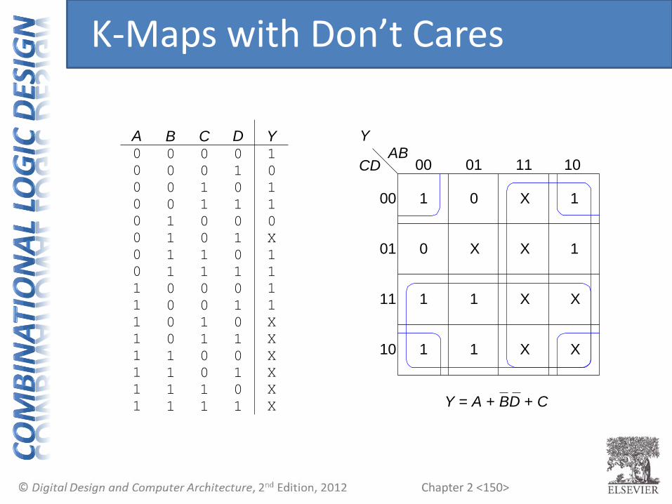
Chapter 2 <150>
0
C D0 0
0 1
1 0
1 1
B0
0
0
0
0 0
0 1
1 0
1 1
1
1
1
1
1
1
1
0
X
1
1
YA0
0
0
0
0
0
0
0
0 0
0 1
1 0
1 1
0
0
0
0
0 0
0 1
1 0
1 1
1
1
1
1
1
1
1
1
1
1
1
1
1
1
X
X
X
X
X
X
01 11
1
0
0
X
X
X
1
101
1
1
1
1
X
X
X
X
11
10
00
00
10AB
CD
Y
Y = A + BD + C
K-Maps with Don’t Cares

Chapter 2 <151>
01 11
1
0
0
1
0
0
1
101
1
1
1
1
0
0
0
1
11
10
00
00
10AB
CD
Y
0
C D0 0
0 1
1 0
1 1
B0
0
0
0
0 0
0 1
1 0
1 1
1
1
1
1
1
1
1
0
1
1
1
YA0
0
0
0
0
0
0
0
0 0
0 1
1 0
1 1
0
0
0
0
0 0
0 1
1 0
1 1
1
1
1
1
1
1
1
1
1
1
1
1
1
1
1
0
0
0
0
0
4-Input K-Map: POS & SOP Form
Chapter 2 <152>
01 11
1
0
0
1
0
0
1
101
1
1
1
1
0
0
0
1
11
10
00
00
10AB
CD
Y
Y = AC + ABD + ABC + BD
0
C D0 0
0 1
1 0
1 1
B0
0
0
0
0 0
0 1
1 0
1 1
1
1
1
1
1
1
1
0
1
1
1
YA0
0
0
0
0
0
0
0
0 0
0 1
1 0
1 1
0
0
0
0
0 0
0 1
1 0
1 1
1
1
1
1
1
1
1
1
1
1
1
1
1
1
1
0
0
0
0
0
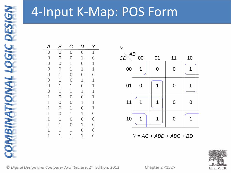
4-Input K-Map: POS Form

Chapter 2 <153>
01 11
1
0
0
1
0
0
1
101
1
1
1
1
0
0
0
1
11
10
00
00
10AB
CD
Y
0
C D0 0
0 1
1 0
1 1
B0
0
0
0
0 0
0 1
1 0
1 1
1
1
1
1
1
1
1
0
1
1
1
YA0
0
0
0
0
0
0
0
0 0
0 1
1 0
1 1
0
0
0
0
0 0
0 1
1 0
1 1
1
1
1
1
1
1
1
1
1
1
1
1
1
1
1
0
0
0
0
0
4-Input K-Map: POS Form

Chapter 2 <154>
• “Add” literal/complement terms to reverse simplification (expand literal)
• Example• 𝑌 = 𝐶
• 𝑌 = 𝐶 + 𝐴 ҧ𝐴
• 𝑌 = 𝐶 + 𝐴 ⋅ (𝐶 + ҧ𝐴)
• 𝑌 = [ 𝐶 + 𝐴 + 𝐵 ത𝐵](𝐶 + ҧ𝐴)
• 𝑌 = 𝐶 + 𝐴 + 𝐵 𝐶 + 𝐴 + ത𝐵 𝐶 + ҧ𝐴
• …
Canonical POS Expansion
Chapter 2 <155>
• Multiplexers
• Decoders
Combinational Building Blocks

Chapter 2 <156>
• Selects between one of N inputs to connect to output
• log2N-bit required to select input – control input S
• Example: 2:1 Mux (2 inputs to 1 output)
• 𝑁 = 2
• log2 2 =1 control bit required
Multiplexer (Mux)
Y
0 0
0 1
1 0
1 1
0
1
0
1
0
0
0
0
0 0
0 1
1 0
1 1
1
1
1
1
0
0
1
1
0
1
S
D0
YD
1
D1
D0
S Y
0
1 D1
D0
S

Chapter 2 <157>
2-<157>
• Logic gates• Sum-of-products form
Y
D0
S
D1
D1
Y
D0
S
S00 01
0
1
Y
11 10
D0
D1
0
0
0
1
1
1
1
0
Y = D0S + D
1S
• Tristates• For an N-input mux, use N
tristates
• Turn on exactly one to select the appropriate input
Multiplexer Implementations

Chapter 2 <158>
A B Y0 0 0
0 1 0
1 0 0
1 1 1
Y = AB
00
Y01
10
11
A B
• Using the mux as a lookup table
• Zero outputs tied to GND
• One output tied to VDD
Logic using Multiplexers

Chapter 2 <159>
A B Y0 0 0
0 1 0
1 0 0
1 1 1
Y = AB
A Y
0
1
0 0
1
A
BY
B
• Reducing the size of the mux
Logic using Multiplexers
Chapter 2 <160>
2:4
Decoder
A1
A0
Y3
Y2
Y1
Y0
00011011
0 0
0 1
1 0
1 1
0
0
0
1
Y3
Y2
Y1
Y0
A0
A1
0
0
1
0
0
1
0
0
1
0
0
0
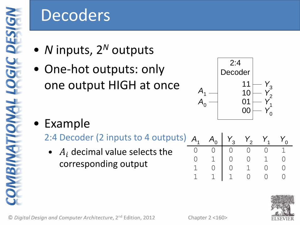
• N inputs, 2N outputs
• One-hot outputs: only one output HIGH at once
• Example2:4 Decoder (2 inputs to 4 outputs)
• 𝐴𝑖 decimal value selects the corresponding output
Decoders

Chapter 2 <161>
Y3
Y2
Y1
Y0
A0A1
Decoder Implementation

Chapter 2 <162>
2:4
Decoder
A
B00011011
Y = AB + AB
Y
ABABABAB
Minterm
= A B
• OR minterms
Logic Using Decoders
XNOR function
Chapter 2 <163>
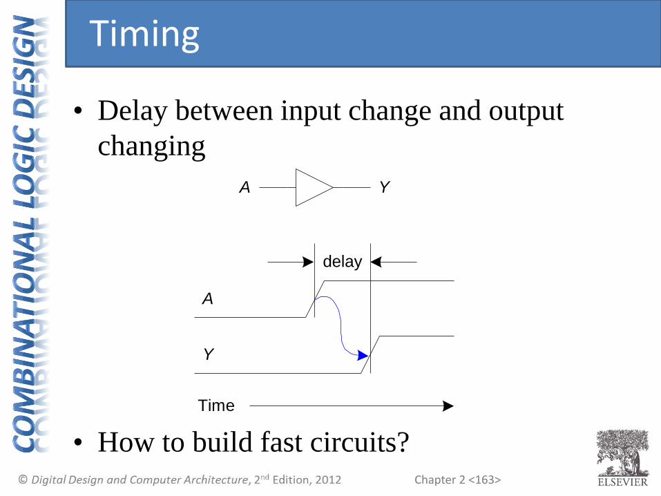
• Delay between input change and output
changing
• How to build fast circuits?
A
Y
Time
delay
A Y
Timing

Chapter 2 <164>
A
Y
Time
A Y
tpd
tcd
• Propagation delay: tpd = max delay from input to final output
• Contamination delay: tcd = min delay from input to initial output
change
Propagation & Contamination Delay
Note: Timing diagram shows a signal with a high and low and transition time as an ‘X’.
Cross hatch indicates unknown/changing values

Chapter 2 <165>
• Delay is caused by
• Capacitance and resistance in a circuit
• Speed of light limitation
• Reasons why tpd and tcd may be different:
• Different rising and falling delays
• Multiple inputs and outputs, some of which are
faster than others
• Circuits slow down when hot and speed up when
cold
Propagation & Contamination Delay
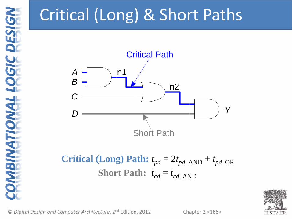
Chapter 2 <166>
AB
C
D Y
Critical Path
Short Path
n1
n2
Critical (Long) Path: tpd = 2tpd_AND + tpd_OR
Short Path: tcd = tcd_AND
Critical (Long) & Short Paths

Chapter 2 <167>
• When a single input change causes an output
to change multiple times
Glitches

Chapter 2 <168>
AB
C
Y
00 01
1
Y
11 10AB
1
1
0
1
0
1
0
0
C
0
Y = AB + BC
• What happens when A = 0, C = 1, B falls?
Glitch Example

Chapter 2 <169>
A = 0B = 1 0
C = 1
Y = 1 0 1
Short Path
Critical Path
B
Y
Time
1 0
0 1
glitch
n1
n2
n2
n1
Glitch Example (cont.)
Note: n1 is slower than n2 because of the extra inverter for B to go through

Chapter 2 <170>
00 01
1
Y
11 10AB
1
1
0
1
0
1
0
0
C
0
Y = AB + BC + ACAC
B = 1 0Y = 1
A = 0
C = 1
Fixing the Glitch
Consensus term

Chapter 2 <171>
• Glitches shouldn’t cause problems because
of synchronous design conventions (see
Chapter 3)
• It’s important to recognize a glitch: in
simulations or on oscilloscope
• Can’t get rid of all glitches – simultaneous
transitions on multiple inputs can also
cause glitches
Why Understand Glitches?


