
CREDIT RISK MEASUREMENT
Classes #14; Chap 11

Lecture Outline
Purpose: Gain a basic understanding of credit risk. Specifically, how it is measured
Measuring Credit Risk Qualitative Factors Quantitative Models
Credit Score Models Value-at-Risk (VaR) RAROC Other models (if time permits)
2
Measuring Loan Credit Risk
3
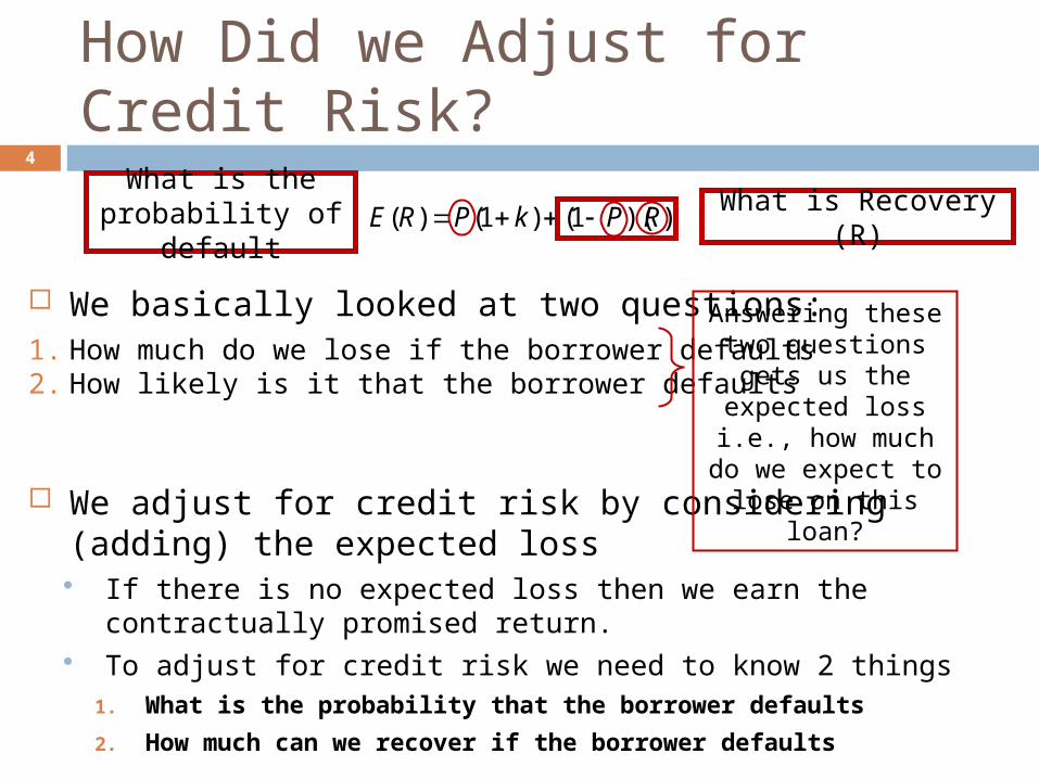
How Did we Adjust for Credit Risk?
We basically looked at two questions:1. How much do we lose if the borrower defaults2. How likely is it that the borrower defaults
We adjust for credit risk by considering (adding) the expected loss If there is no expected loss then we earn the contractually promised return. To adjust for credit risk we need to know 2 things
1. What is the probability that the borrower defaults
2. How much can we recover if the borrower defaults
4
))(1()1()( RPkPRE
Answering these two questions gets us the
expected loss i.e., how much do we expect to
lose on this loan?
What is Recovery (R)What is the
probability of default

Adjusting for Credit Risk
In the credit risk game we need good estimates of:
1.The loan’s probability of default
2.The recovery in default
3.The expected loss Instead of estimating the probability of default and recovery separately
we can take them together and estimate the expected loss directly
5
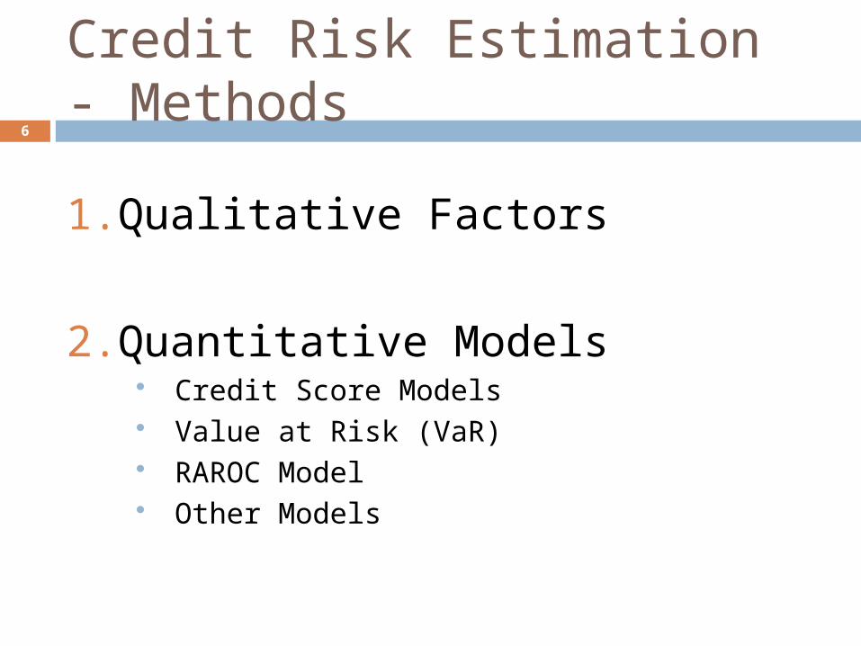
Credit Risk Estimation - Methods
1.Qualitative Factors
2.Quantitative Models Credit Score Models Value at Risk (VaR) RAROC Model Other Models
6
Qualitative Factors
7
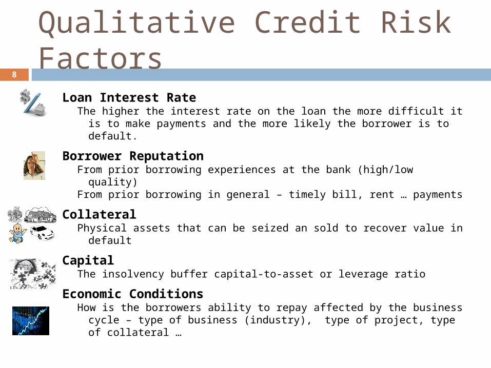
Qualitative Credit Risk Factors
Loan Interest RateThe higher the interest rate on the loan the more difficult it is to make
payments and the more likely the borrower is to default.
Borrower ReputationFrom prior borrowing experiences at the bank (high/low quality)From prior borrowing in general – timely bill, rent … payments
CollateralPhysical assets that can be seized an sold to recover value in default
CapitalThe insolvency buffer capital-to-asset or leverage ratio
Economic ConditionsHow is the borrowers ability to repay affected by the business cycle –
type of business (industry), type of project, type of collateral …
8
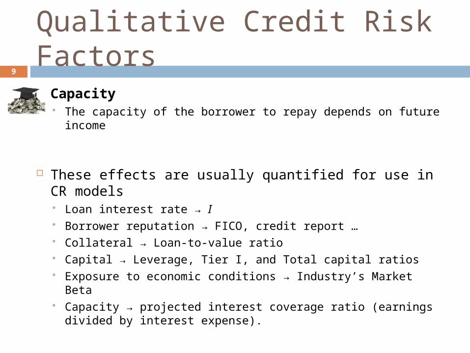
Capacity The capacity of the borrower to repay depends on future income
These effects are usually quantified for use in CR models Loan interest rate → I Borrower reputation → FICO, credit report … Collateral → Loan-to-value ratio Capital → Leverage, Tier I, and Total capital ratios Exposure to economic conditions → Industry’s Market Beta Capacity → projected interest coverage ratio (earnings divided by
interest expense).
9
Qualitative Credit Risk Factors
Quantitative Models of Credit Risk Credit Score Models Value at Risk (VaR) RAROC Model Other Models
10

Credit Score Model Linear Probability Model Logit Analysis Linear Discriminate Model
11
Credit Score Model
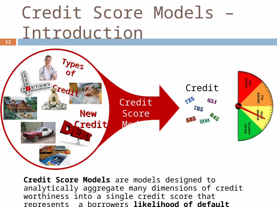
Credit Score Models – Introduction12
Types ofTypes of CreditCredit
Credit Score Models are models designed to analytically aggregate many dimensions of credit worthiness into a single credit score that represents a borrowers likelihood of default
New New CreditCredit
Credit Score
13
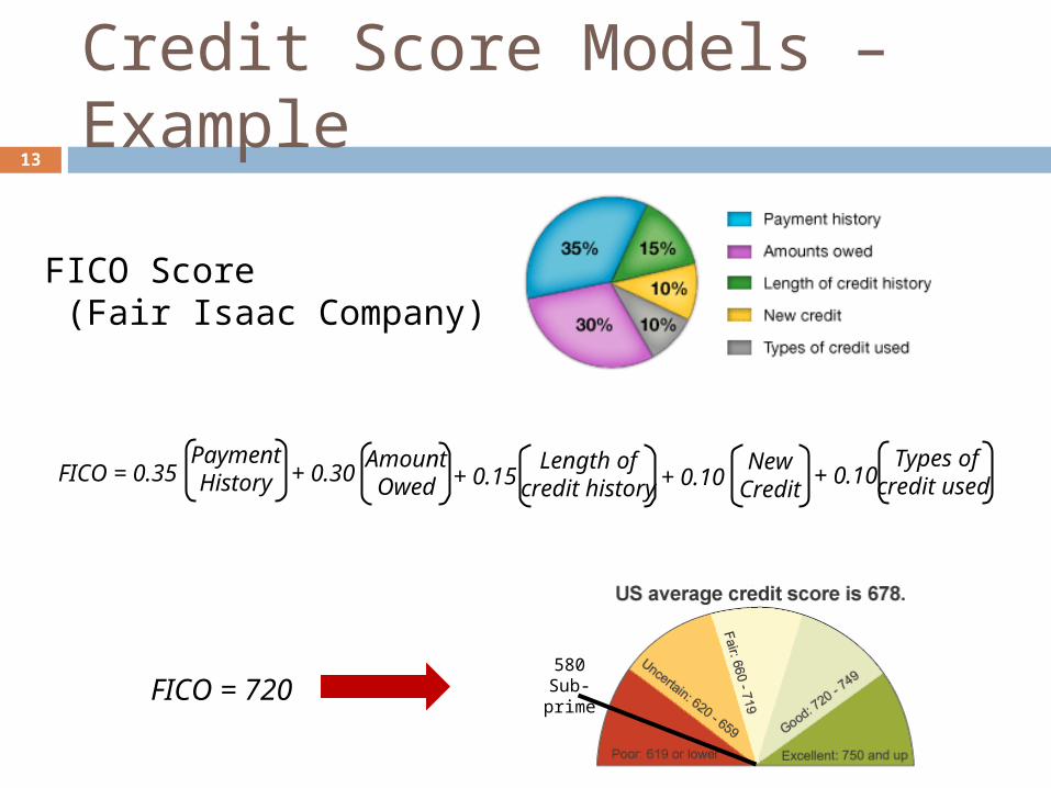
Credit Score Models – Example
FICO Score (Fair Isaac Company)
FICO = 0.35Payment History + 0.30
Amount Owed + 0.15 + 0.10 + 0.10
New Credit
Length of credit history
Types of credit used
FICO = 720580
Sub-prime
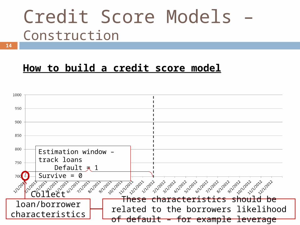
How to build a credit score model
14
Credit Score Models – Construction
Estimation window – track loans Default = 1 Survive = 0
These characteristics should be related to the borrowers likelihood of default – for example leverage
Collect loan/borrower characteristics
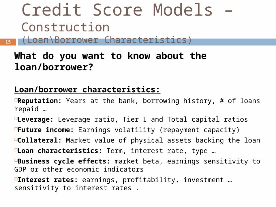
What do you want to know about the loan/borrower?
Loan/borrower characteristics:Reputation: Years at the bank, borrowing history, # of loans repaid … Leverage: Leverage ratio, Tier I and Total capital ratios Future income: Earnings volatility (repayment capacity)Collateral: Market value of physical assets backing the loanLoan characteristics: Term, interest rate, type …Business cycle effects: market beta, earnings sensitivity to GDP or other economic indicatorsInterest rates: earnings, profitability, investment … sensitivity to interest rates .
15
Credit Score Models – Construction(Loan\Borrower Characteristics)

16
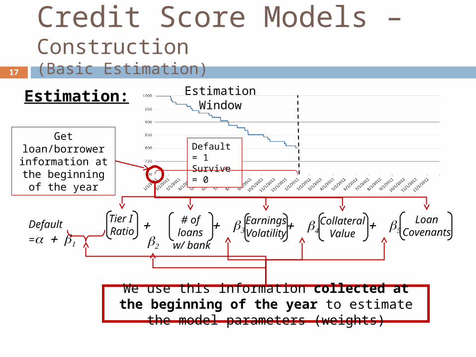
Credit Score Models – Construction(Basic Estimation)
Default = 1Survive = 0
Estimation: Estimation Window
Object is to build a model that we can use to predict default in the next period
17
Credit Score Models – Construction(Basic Estimation)
Default = 1Survive = 0
Estimation: Estimation Window
We use this information collected at the beginning of the year to estimate the model parameters (weights)
Tier I Ratio
# of loans w/ bank
Collateral Value
Earnings Volatility
Loan Covenants
Default
=
Get loan/borrower information at the
beginning of the year

18
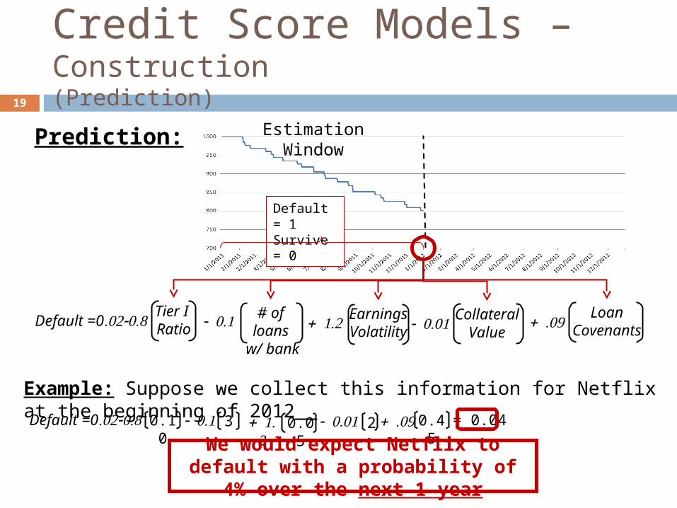
Credit Score Models – Construction (Prediction)
Default = 1Survive = 0
Prediction: Estimation Window
Tier I Ratio
# of loans w/ bank
Collateral Value
Earnings Volatility
Loan Covenants
Default
=
Default =0
After estimating the model, we can fill in the parameters and the model can be used to forecast loan/borrower defaults
19
Credit Score Models – Construction(Prediction)
Default = 1Survive = 0
Prediction: Estimation Window
Tier I Ratio
# of loans w/ bank
Collateral Value
Earnings Volatility
Loan Covenants
Default =0
Default =0
0.10 3 0.05 2 0.45 = 0.04
Example: Suppose we collect this information for Netflix at the beginning of 2012
We would expect Netflix to default with a probability of 4% over the next 1 year
20
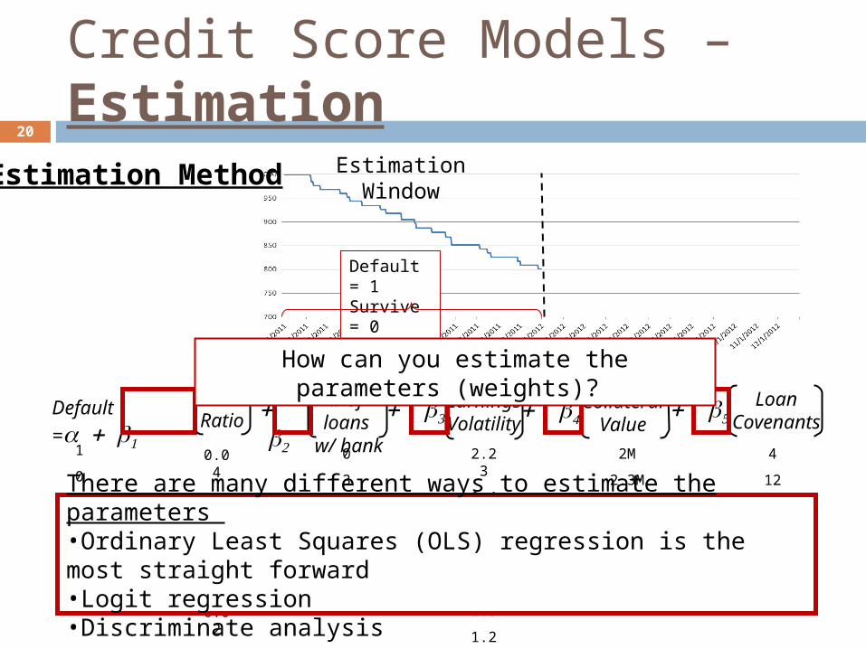
Credit Score Models – Estimation
Default = 1Survive = 0
Estimation Method Estimation Window
Default
=
Tier I Ratio
# of loans w/ bank
Collateral Value
Earnings Volatility
Loan Covenants
1
0
⁞
1
0
0
0.04
0.07
⁞
0.10
0.02
0.05
0
3
⁞
7
2
0
2.23
0.45
⁞
1.23
2.8
1.2
2M
2.3M
⁞
0.32M
0.8M
5.2M
4
12
⁞
8
6
3
How can you estimate the parameters (weights)?
There are many different ways to estimate the parameters •Ordinary Least Squares (OLS) regression is the most straight forward•Logit regression•Discriminate analysis
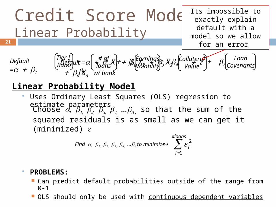
Linear Probability Model Uses Ordinary Least Squares (OLS) regression to estimate parameters
PROBLEMS: Can predict default probabilities outside of the range from 0-1 OLS should only be used with continuous dependent variables
21
Credit Score Models – Linear Probability
Default
=
Tier I Ratio
# of loans w/ bank
Collateral Value
Earnings Volatility
Loan Covenants
Default =X1X2X3 …nXn
Choose …n,so that the sum of the squared residuals is as small as we can get it (minimized)
loans
ii
#
1
2Find…n to minimize
Its impossible to exactly explain default with a model
so we allow for an error
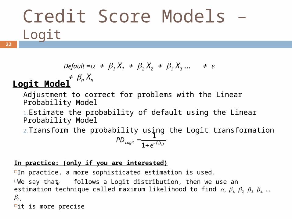
Logit ModelAdjustment to correct for problems with the Linear Probability Model1.Estimate the probability of default using the Linear Probability Model2.Transform the probability using the Logit transformation
22
Credit Score Models – Logit
Default =X1X2X3 …nXn
LPPDLogit ePD
1
1
In practice: (only if you are interested)In practice, a more sophisticated estimation is used.We say that follows a Logit distribution, then we use an estimation technique called maximum likelihood to find …n,it is more precise
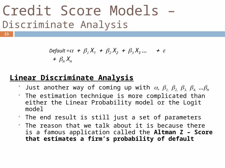
Linear Discriminate Analysis Just another way of coming up with …n The estimation technique is more complicated than either the Linear
Probability model or the Logit model The end result is still just a set of parameters The reason that we talk about it is because there is a famous application
called the Altman Z – Score that estimates a firm’s probability of default
23
Credit Score Models – Discriminate Analysis
Default =X1X2X3 …nXn
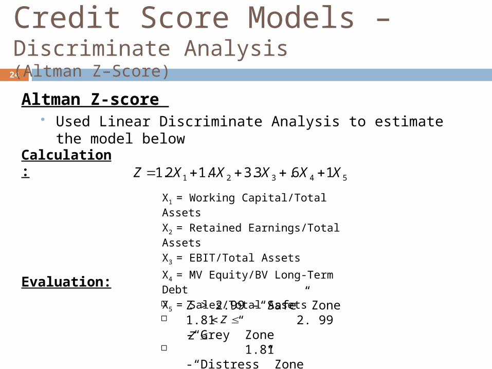
Altman Z-score Used Linear Discriminate Analysis to estimate the model below
24
Credit Score Models – Discriminate Analysis(Altman Z–Score)
54321 16.3.34.12.1 XXXXXZ
X1 = Working Capital/Total Assets
X2 = Retained Earnings/Total Assets
X3 = EBIT/Total Assets
X4 = MV Equity/BV Long-Term Debt
X5 = Sales/Total Assets
Z > 2.99 -“Safe” Zone 1.81 2. 99 -“Grey” Zone 1.81 -“Distress” Zone
Z
Z
Calculation:
Evaluation:

Kaplan Associates has estimated the following linear probability model using loan defaults over the past 4 years.
Suppose that North Star restaurant applies for a loan. They have a leverage ratio of 0.25, a FICO score of 720 and a 10 year credit history.
25
) (032.0)(0085.0)(003.0001.0 historycreditoflengthFICOLeveragePD
a) Calculate the probability that North Star defaults over the next year using the linear probability modelb) Calculate the probability that North Star defaults over the next four years using the linear probability modelc) Calculate the probability that North Star defaults over the next four years using the Logit model
11-26
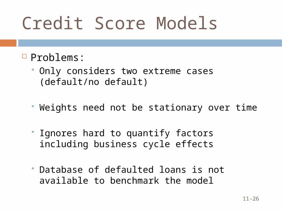
Credit Score Models
Problems: Only considers two extreme cases (default/no default)
Weights need not be stationary over time
Ignores hard to quantify factors including business cycle effects
Database of defaulted loans is not available to benchmark the model

Value at Risk (VaR)
27
Thinking About Credit Risk
What have we done so far: Followed a group of firms – some defaulted and some did not. Used the actual defaults vs. non-default to try to understand, in
general, what causes a firm to default on its loans. Problem - we have to wait for firms to default to understand what
causes default
Another way of thinking: If no firms defaulted would that mean that there is no credit risk? The value of a loan can change simply because the probability of
default or what we expect to recover in default changes. This is credit risk! It exists even if no firms default Value-at-Risk is one method used to measure this
28
VaR asks: Based on what has happened in the past On a really bad day, how much will I lose on my loan position?
How to answer this question:1. Collect past returns – for example, one year of daily returns2. Calculate the mean and standard deviations of daily returns3. Assume a normal distribution4. Declare a significance level – for example 99%5. Find the Value-at-risk (VaR) – Value that the company’s losses will
exceed only 1% of the time – over the return horizon (next day)
29
Value-at-Risk (VaR) – Concept
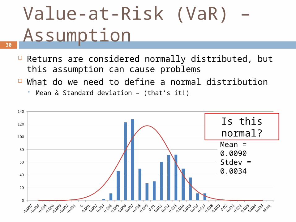
Returns are considered normally distributed, but this assumption can cause problems
What do we need to define a normal distribution Mean & Standard deviation – (that’s it!)
30
Value-at-Risk (VaR) – Assumption
Mean = 0.0090Stdev = 0.0034
Is this normal?
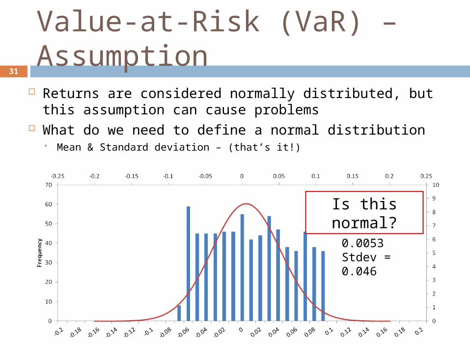
Returns are considered normally distributed, but this assumption can cause problems
What do we need to define a normal distribution Mean & Standard deviation – (that’s it!)
31
Value-at-Risk (VaR) – Assumption
Mean = 0.0053Stdev = 0.046
Is this normal?
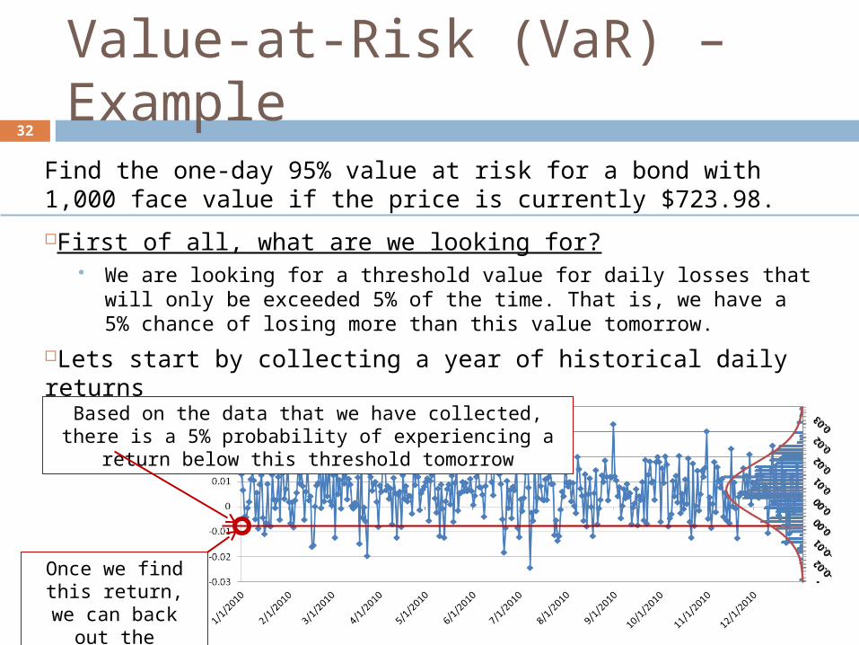
Find the one-day 95% value at risk for a bond with 1,000 face value if the price is currently $723.98.
First of all, what are we looking for? We are looking for a threshold value for daily losses that will only be exceeded 5% of
the time. That is, we have a 5% chance of losing more than this value tomorrow.
Lets start by collecting a year of historical daily returns We work with returns because they are usually normally distributed – prices are not!
32
Value-at-Risk (VaR) – Example
Based on the data that we have collected, there is a 5% probability of experiencing a return below this threshold tomorrow
Once we find this return, we can back out the VaR(95%)

Find the one-day 95% value at risk for a bond with 1,000 face value if the price is currently $723.98.
Step #1: Calculate the mean and standard deviation
Step #2: Find the 95% VaR
33
Value-at-Risk (VaR) – Example
Mean = 0.005473Stdev = 0.009128
Mean = 0.005473Stdev = 0.009128
We want to find the return that gives us 5% of the area under the curve in the tail
5%How do you do it?
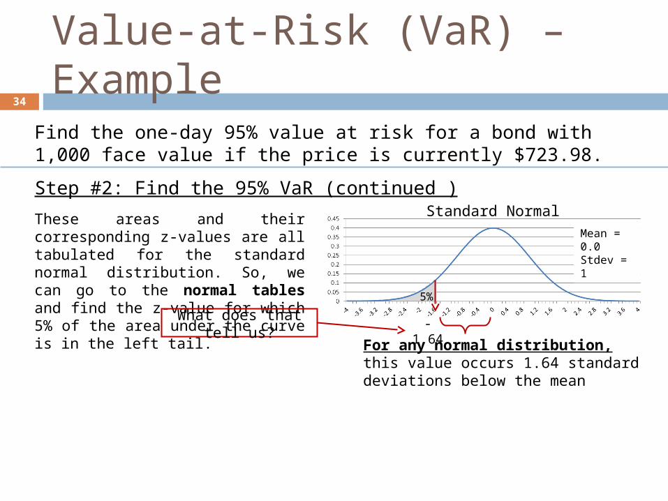
Find the one-day 95% value at risk for a bond with 1,000 face value if the price is currently $723.98.
Step #2: Find the 95% VaR (continued )Standard Normal
5%
Mean = 0.0Stdev = 1
34
Value-at-Risk (VaR) – Example
These areas and their corresponding z-values are all tabulated for the standard normal distribution. So, we can go to the normal tables and find the z-value for which 5% of the area under the curve is in the left tail.
-1.64What does that tell us?
For any normal distribution, this value occurs 1.64 standard deviations below the mean

Find the one-day 95% value at risk for a bond with 1,000 face value if the price is currently $723.98.
Step #2: Find the 95% VaR (continued )Standard Normal
5%
Mean = 0.0Stdev = 1
35
Value-at-Risk (VaR) – Example
These areas and their corresponding z-values are all tabulated for the standard normal distribution. So, we can go to the normal tables and find the z-value for which 5% of the area under the curve is in the left tail.
-1.64
Mean = 0.005473Stdev = 0.009128
5%
Our Distribution
X
We know that “X” is 1.64 standard deviations below the mean
X = 0.005473
Start at the mean subtract 1.64 Standard deviations in this case 0.009128
– 1.64(0.009128) = -0.0095
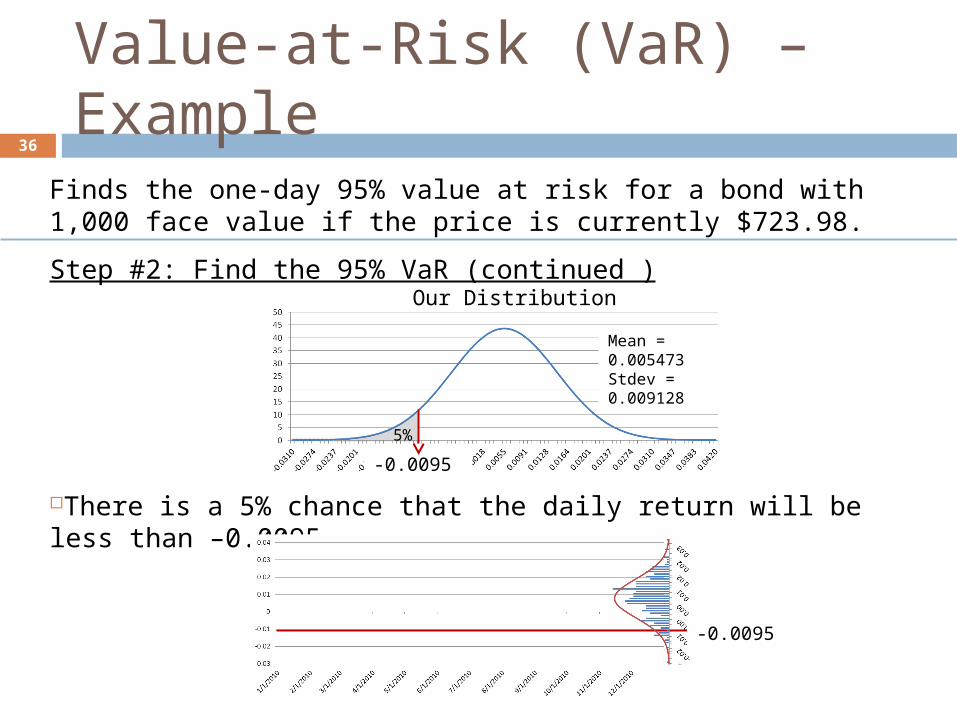
Finds the one-day 95% value at risk for a bond with 1,000 face value if the price is currently $723.98.
Step #2: Find the 95% VaR (continued )
There is a 5% chance that the daily return will be less than –0.0095
36
Value-at-Risk (VaR) – Example
Mean = 0.005473Stdev = 0.009128
5%
Our Distribution
X-0.0095
-0.0095
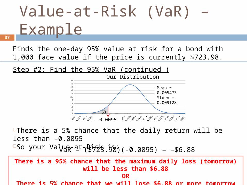
Finds the one-day 95% value at risk for a bond with 1,000 face value if the price is currently $723.98.
Step #2: Find the 95% VaR (continued )
There is a 5% chance that the daily return will be less than –0.0095 So your Value-at-Risk is:
37
Value-at-Risk (VaR) – Example
Mean = 0.005473Stdev = 0.009128
5%
Our Distribution
X-0.0095
VaR = ($723.98)(-0.0095) = –$6.88
There is a 95% chance that the maximum daily loss (tomorrow) will be less than $6.88OR
There is 5% chance that we will lose $6.88 or more tomorrow

Lorden Investments has a loan portfolio with a current value of $172M . The mean an variance of the value weighted daily return on their portfolio is 0.0181 and 0.0004 respectively. Find the 99% value at risk for the loan portfolio
38
2.33
RAROC Model
39
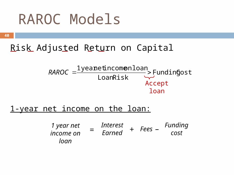
RAROC Models
Risk Adjusted Return on Capital
1-year net income on the loan:
40
1 year net income on loan
Interest Earned
FeesFunding
cost= – +
Costs FundingRiskLoan
loan on incomenet year 1RAROC
Accept loan
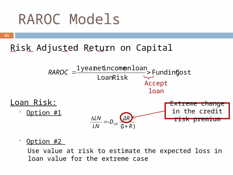
RAROC Models
Risk Adjusted Return on Capital
Loan Risk: Option #1
Option #2
Use value at risk to estimate the expected loss in loan value for the extreme case
41
)1( R
ΔR -D
LN
LNLN
Extreme change in the credit risk premium
Costs FundingRiskLoan
loan on incomenet year 1RAROC
Accept loan
42
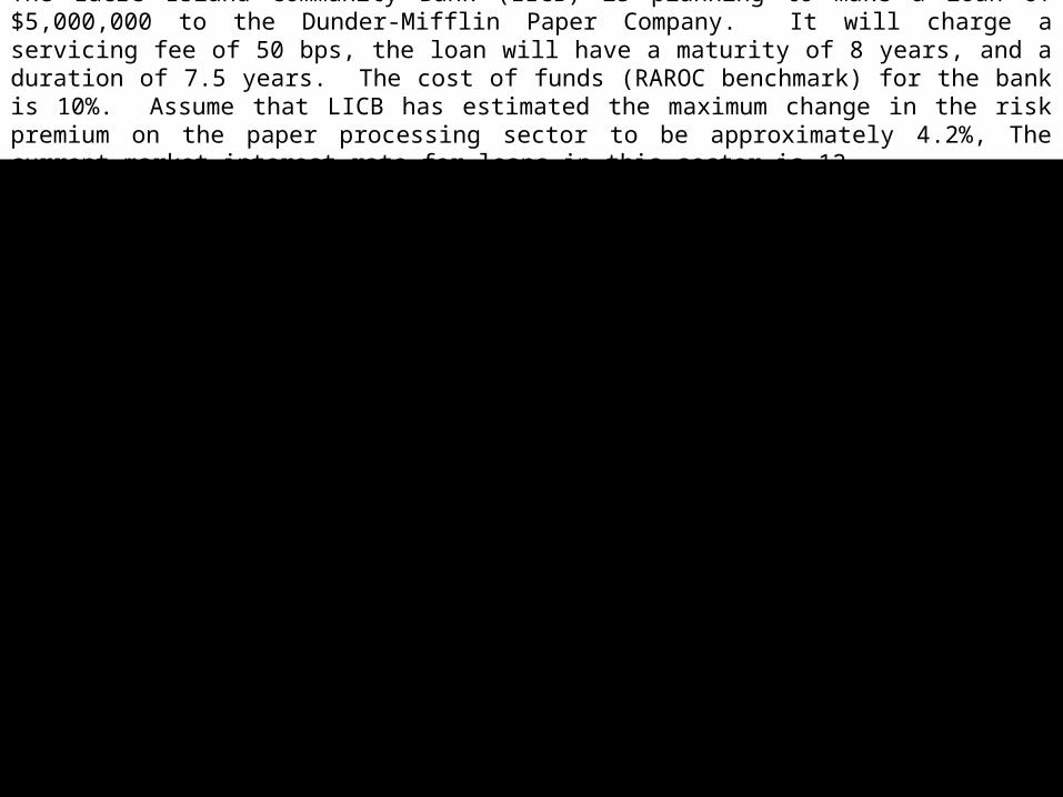
The Lucre Island Community Bank (LICB) is planning to make a loan of $5,000,000 to the Dunder-Mifflin Paper Company. It will charge a servicing fee of 50 bps, the loan will have a maturity of 8 years, and a duration of 7.5 years. The cost of funds (RAROC benchmark) for the bank is 10%. Assume that LICB has estimated the maximum change in the risk premium on the paper processing sector to be approximately 4.2%, The current market interest rate for loans in this sector is 12
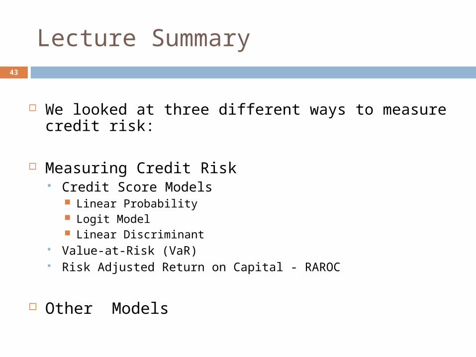
Lecture Summary43
We looked at three different ways to measure credit risk:
Measuring Credit Risk Credit Score Models
Linear Probability Logit Model Linear Discriminant
Value-at-Risk (VaR) Risk Adjusted Return on Capital - RAROC
Other Models

AppendixOther Models
44

11-45
Term Structure Based Methods
We can use the credit spread in the market to determine the level of risk probability of default using zero coupons and strips
Suppose the contractual promised return on a corporate bond is k –the expected return is then
p (1+ k)+(1-p)(0)
Assuming zero recovery
Suppose the FI require a return equal to the risk free rate i
p (1+ k)+(1-p)(0)= 1+i
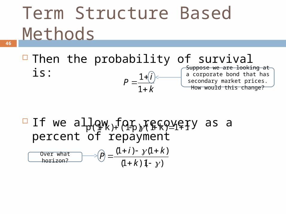
Term Structure Based Methods
Then the probability of survival is:
If we allow for recovery as a percent of repayment
46
k
iP
1
1
i1 k)(1p)-(1k)p(1
)1)(1(
)1()1(
k
kiP
Suppose we are looking at a corporate bond that has
secondary market prices. How would this change?
Over what horizon?
11-47
Term Structure Based Methods
May be generalized to loans with any maturity or to adjust for varying default recovery rates
The loan can be assessed using the inferred probabilities from comparable quality bonds
11-48
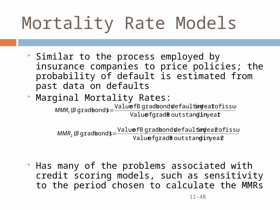
Mortality Rate Models
Similar to the process employed by insurance companies to price policies; the probability of default is estimated from past data on defaults
Marginal Mortality Rates:
Has many of the problems associated with credit scoring models, such as sensitivity to the period chosen to calculate the MMRs
1year in goutstandin B grade of Value
issue of 1year in defaulted bonds grade B of Value)bonds grade (1 BMMR
2year in goutstandin B grade of Value
issue of 2year in defaulted bonds grade B of Value)bonds grade (2 BMMR
11-49
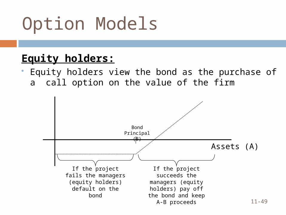
Option Models
Equity holders: Equity holders view the bond as the purchase of a call option on the
value of the firm
Bond Principal (B)
If the project fails the managers (equity holders)
default on the bond
If the project succeeds the managers (equity holders) pay off the bond and keep
A-B proceeds
Assets (A)
11-50
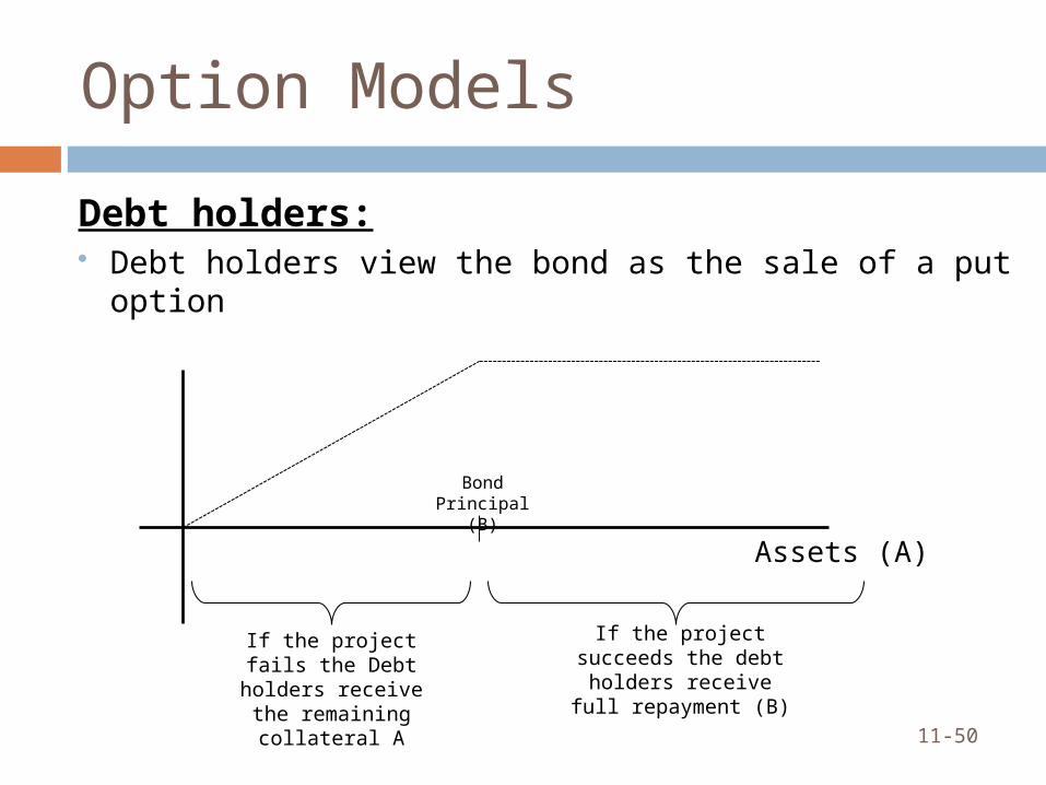
Option Models
Debt holders: Debt holders view the bond as the sale of a put option
Bond Principal (B)
If the project fails the Debt holders receive the
remaining collateral A
If the project succeeds the debt holders receive full
repayment (B)
Assets (A)

11-51
Applying Option Valuation Model
Merton showed value of a risky loan:
where
F() = value of risky debt
ln = Natural logarithm
i = Risk-free rate on debt of equivalent maturity
remaining time to maturity
B = principal amount on the bond
)()()( 21 hNhNBeBeF ii
)/ln(2
1
ABeh
i
)/ln(2
2
ABeh
i


