

CS6220: DATA MINING TECHNIQUES
Instructor: Yizhou [email protected]
September 14, 2014
Matrix Data: Classification: Part 1
Matrix Data: Classification: Part 1
•Classification: Basic Concepts
•Decision Tree Induction
•Model Evaluation and Selection
• Summary
2
Supervised vs. Unsupervised Learning
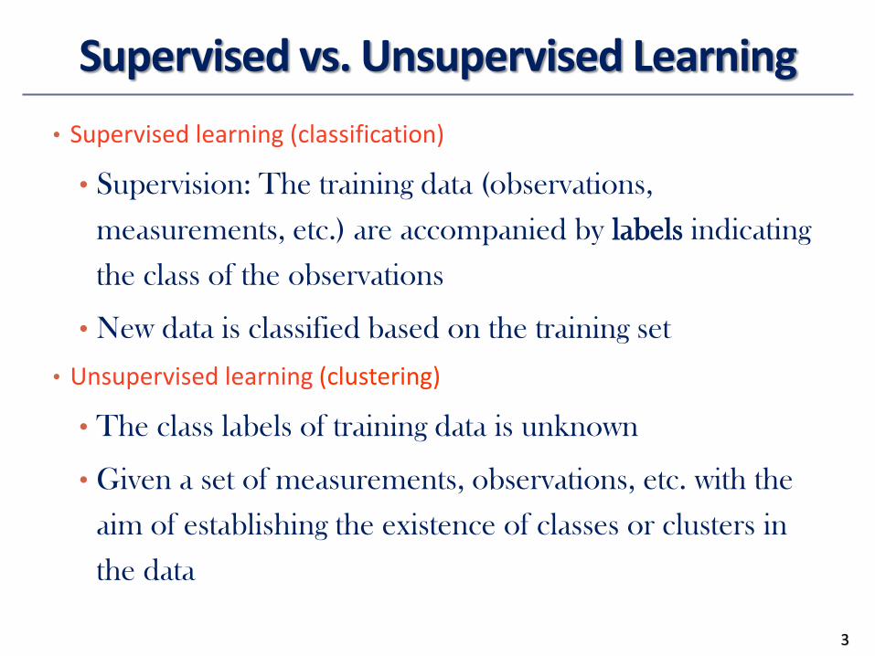
• Supervised learning (classification)
• Supervision: The training data (observations,
measurements, etc.) are accompanied by labels indicating
the class of the observations
• New data is classified based on the training set
• Unsupervised learning (clustering)
• The class labels of training data is unknown
• Given a set of measurements, observations, etc. with the
aim of establishing the existence of classes or clusters in
the data
3

Prediction Problems: Classification vs. Numeric Prediction
• Classification
• predicts categorical class labels
• classifies data (constructs a model) based on the training set and the values (class labels) in a classifying attribute and uses it in classifying new data
• Numeric Prediction
• models continuous-valued functions, i.e., predicts unknown or missing values
• Typical applications
• Credit/loan approval:
• Medical diagnosis: if a tumor is cancerous or benign
• Fraud detection: if a transaction is fraudulent
• Web page categorization: which category it is
4

Classification—A Two-Step Process (1)
• Model construction: describing a set of predetermined classes
• Each tuple/sample is assumed to belong to a
predefined class, as determined by the class label
attribute
• For data point i: < 𝒙𝒊, 𝑦𝑖 >
• Features: 𝒙𝒊; class label: 𝑦𝑖
• The model is represented as classification rules,
decision trees, or mathematical formulae
• Also called classifier
• The set of tuples used for model construction is
training set
5

Classification—A Two-Step Process (2)
• Model usage: for classifying future or unknown objects
• Estimate accuracy of the model
• The known label of test sample is compared with the classified result from the model
• Test set is independent of training set (otherwise overfitting)
• Accuracy rate is the percentage of test set samples that are correctly classified by the model
• Most used for binary classes
• If the accuracy is acceptable, use the model to classify new data
• Note: If the test set is used to select models, it is called validation (test) set
6

Process (1): Model Construction
7
Training
Data
NAME RANK YEARS TENURED
Mike Assistant Prof 3 no
Mary Assistant Prof 7 yes
Bill Professor 2 yes
Jim Associate Prof 7 yes
Dave Assistant Prof 6 no
Anne Associate Prof 3 no
Classification
Algorithms
IF rank = ‘professor’
OR years > 6
THEN tenured = ‘yes’
Classifier
(Model)
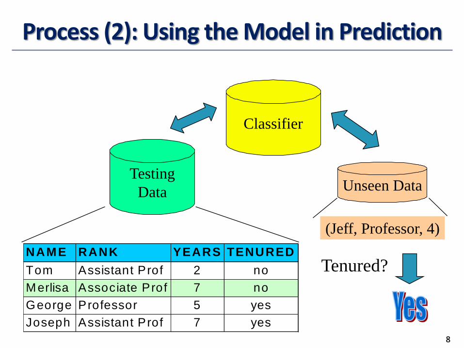
Process (2): Using the Model in Prediction
8
Classifier
Testing
Data
NAME RANK YEARS TENURED
Tom Assistant Prof 2 no
Merlisa Associate Prof 7 no
George Professor 5 yes
Joseph Assistant Prof 7 yes
Unseen Data
(Jeff, Professor, 4)
Tenured?
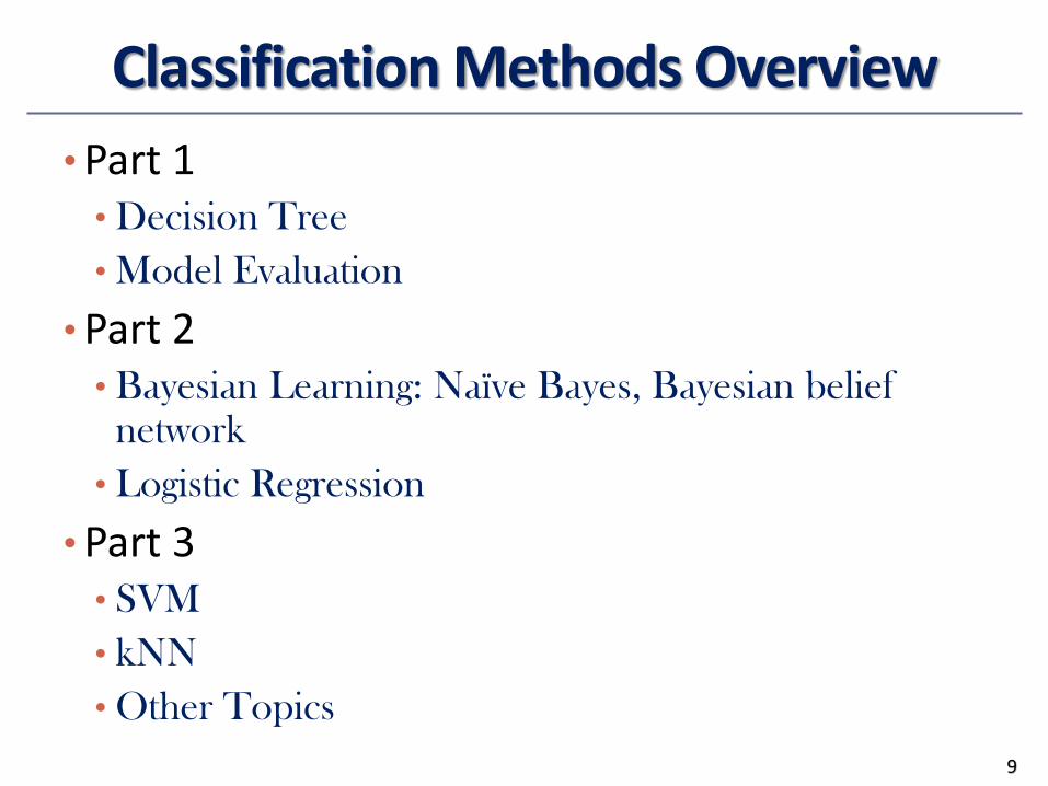
Classification Methods Overview
•Part 1• Decision Tree
• Model Evaluation
•Part 2• Bayesian Learning: Naïve Bayes, Bayesian belief
network
• Logistic Regression
•Part 3• SVM
• kNN
• Other Topics
9
Matrix Data: Classification: Part 1
•Classification: Basic Concepts
•Decision Tree Induction
•Model Evaluation and Selection
• Summary
10
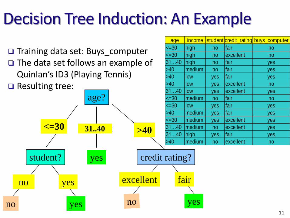
Decision Tree Induction: An Example
11
age?
overcast
student? credit rating?
<=30 >40
no yes yes
yes
31..40
fairexcellentyesno
age income student credit_rating buys_computer
<=30 high no fair no
<=30 high no excellent no
31…40 high no fair yes
>40 medium no fair yes
>40 low yes fair yes
>40 low yes excellent no
31…40 low yes excellent yes
<=30 medium no fair no
<=30 low yes fair yes
>40 medium yes fair yes
<=30 medium yes excellent yes
31…40 medium no excellent yes
31…40 high yes fair yes
>40 medium no excellent no
Training data set: Buys_computer The data set follows an example of
Quinlan’s ID3 (Playing Tennis) Resulting tree:

Algorithm for Decision Tree Induction
• Basic algorithm (a greedy algorithm)• Tree is constructed in a top-down recursive divide-and-conquer
manner• At start, all the training examples are at the root• Attributes are categorical (if continuous-valued, they are discretized
in advance)• Examples are partitioned recursively based on selected attributes• Test attributes are selected on the basis of a heuristic or statistical
measure (e.g., information gain)
• Conditions for stopping partitioning• All samples for a given node belong to the same class• There are no remaining attributes for further partitioning –
majority voting is employed for classifying the leaf• There are no samples left – use majority voting in the parent
partition
12

Brief Review of Entropy
• Entropy (Information Theory)• A measure of uncertainty (impurity) associated with a
random variable
• Calculation: For a discrete random variable Y taking
m distinct values {𝑦1, … , 𝑦𝑚},• 𝐻 𝑌 = − 𝑖=1
𝑚 𝑝𝑖log(𝑝𝑖) , where 𝑝𝑖 = 𝑃(𝑌 = 𝑦𝑖)
• Interpretation:
• Higher entropy => higher uncertainty
• Lower entropy => lower uncertainty
•Conditional Entropy
•𝐻 𝑌 𝑋 = 𝑥 𝑝 𝑥 𝐻(𝑌|𝑋 = 𝑥)m = 2
13

14
Attribute Selection Measure: Information Gain (ID3/C4.5)
Select the attribute with the highest information gain
Let pi be the probability that an arbitrary tuple in D belongs to
class Ci, estimated by |Ci, D|/|D|
Expected information (entropy) needed to classify a tuple in D:
Information needed (after using A to split D into v partitions) to
classify D:
Information gained by branching on attribute A
)(log)( 2
1
i
m
i
i ppDInfo
)(||
||)(
1
j
v
j
j
A DInfoD
DDInfo
(D)InfoInfo(D)Gain(A) A
Attribute Selection: Information Gain
Class P: buys_computer = “yes”
Class N: buys_computer = “no”
means “age <=30” has 5 out of
14 samples, with 2 yes’es and 3
no’s. Hence
Similarly,
15
age pi ni I(pi, ni)
<=30 2 3 0.971
31…40 4 0 0
>40 3 2 0.971
694.0)2,3(14
5
)0,4(14
4)3,2(
14
5)(
I
IIDInfoage
048.0)_(
151.0)(
029.0)(
ratingcreditGain
studentGain
incomeGain
246.0)()()( DInfoDInfoageGain age
age income student credit_rating buys_computer
<=30 high no fair no
<=30 high no excellent no
31…40 high no fair yes
>40 medium no fair yes
>40 low yes fair yes
>40 low yes excellent no
31…40 low yes excellent yes
<=30 medium no fair no
<=30 low yes fair yes
>40 medium yes fair yes
<=30 medium yes excellent yes
31…40 medium no excellent yes
31…40 high yes fair yes
>40 medium no excellent no
)3,2(14
5I
940.0)14
5(log
14
5)
14
9(log
14
9)5,9()( 22 IDInfo
15

Attribute Selection for a Branch
•
16
age?
overcast
? ?
<=30 >40
yes
31..40
Which attribute next?
age income student credit_rating buys_computer
<=30 high no fair no
<=30 high no excellent no
<=30 medium no fair no
<=30 low yes fair yes
<=30 medium yes excellent yes
𝐷𝑎𝑔𝑒≤30
• 𝐼𝑛𝑓𝑜 𝐷𝑎𝑔𝑒≤30 = −2
5log2
2
5−3
5log2
3
5= 0.971
• 𝐺𝑎𝑖𝑛𝑎𝑔𝑒≤30 𝑖𝑛𝑐𝑜𝑚𝑒
= 𝐼𝑛𝑓𝑜 𝐷𝑎𝑔𝑒≤30 − 𝐼𝑛𝑓𝑜𝑖𝑛𝑐𝑜𝑚𝑒 𝐷𝑎𝑔𝑒≤30 = 0.571
• 𝐺𝑎𝑖𝑛𝑎𝑔𝑒≤30 𝑠𝑡𝑢𝑑𝑒𝑛𝑡 = 0.971
• 𝐺𝑎𝑖𝑛𝑎𝑔𝑒≤30 𝑐𝑟𝑒𝑑𝑖𝑡_𝑟𝑎𝑡𝑖𝑛𝑔 = 0.02
age?
overcast
student? ?
<=30 >40
no yes
yes
31..40
yesno

Computing Information-Gain for Continuous-Valued Attributes
• Let attribute A be a continuous-valued attribute
• Must determine the best split point for A
• Sort the value A in increasing order
• Typically, the midpoint between each pair of adjacent values is
considered as a possible split point
• (ai+ai+1)/2 is the midpoint between the values of ai and ai+1
• The point with the minimum expected information requirement
for A is selected as the split-point for A
• Split:
• D1 is the set of tuples in D satisfying A ≤ split-point, and D2 is the
set of tuples in D satisfying A > split-point
17
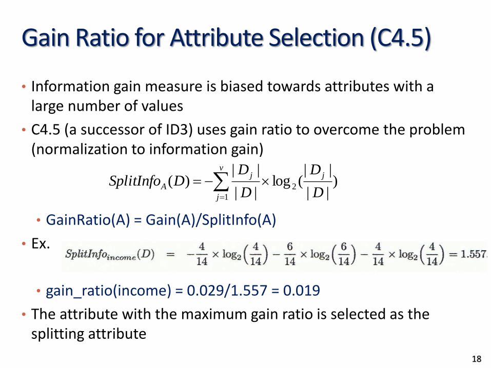
Gain Ratio for Attribute Selection (C4.5)
• Information gain measure is biased towards attributes with a large number of values
• C4.5 (a successor of ID3) uses gain ratio to overcome the problem (normalization to information gain)
• GainRatio(A) = Gain(A)/SplitInfo(A)
• Ex.
• gain_ratio(income) = 0.029/1.557 = 0.019
• The attribute with the maximum gain ratio is selected as the splitting attribute
)||
||(log
||
||)( 2
1 D
D
D
DDSplitInfo
jv
j
j
A
18

Gini Index (CART, IBM IntelligentMiner)
• If a data set D contains examples from n classes, gini index, gini(D) is defined as
where pj is the relative frequency of class j in D
• If a data set D is split on A into two subsets D1 and D2, the giniindex gini(D) is defined as
• Reduction in Impurity:
• The attribute provides the smallest ginisplit(D) (or the largest reduction in impurity) is chosen to split the node (need to enumerate all the possible splitting points for each attribute)
)()()( DginiDginiAginiA
v
j
p jDgini
1
21)(
)(||
||)(
||
||)( 2
21
1Dgini
D
DDgini
D
DDginiA
19

Computation of Gini Index
• Ex. D has 9 tuples in buys_computer = “yes” and 5 in “no”
• Suppose the attribute income partitions D into 10 in D1: {low, medium} and 4 in D2
Gini{low,high} is 0.458; Gini{medium,high} is 0.450. Thus, split on the {low,medium} (and {high}) since it has the lowest Gini index
459.014
5
14
91)(
22
Dgini
)(14
4)(
14
10)( 21},{ DGiniDGiniDgini mediumlowincome
20
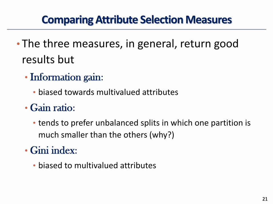
Comparing Attribute Selection Measures
• The three measures, in general, return good
results but
• Information gain:
• biased towards multivalued attributes
• Gain ratio:
• tends to prefer unbalanced splits in which one partition is
much smaller than the others (why?)
• Gini index:
• biased to multivalued attributes
21
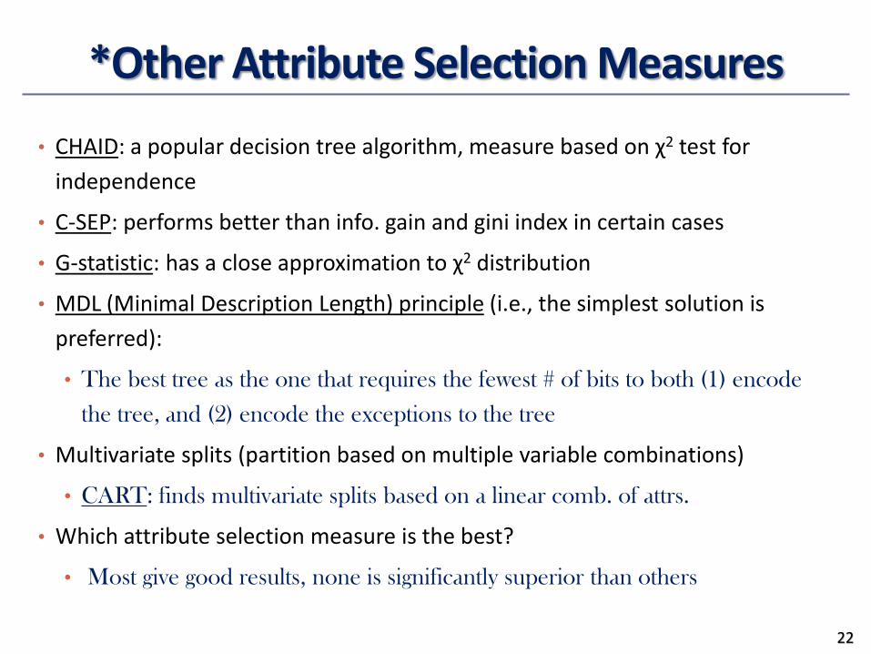
*Other Attribute Selection Measures
• CHAID: a popular decision tree algorithm, measure based on χ2 test for
independence
• C-SEP: performs better than info. gain and gini index in certain cases
• G-statistic: has a close approximation to χ2 distribution
• MDL (Minimal Description Length) principle (i.e., the simplest solution is
preferred):
• The best tree as the one that requires the fewest # of bits to both (1) encode
the tree, and (2) encode the exceptions to the tree
• Multivariate splits (partition based on multiple variable combinations)
• CART: finds multivariate splits based on a linear comb. of attrs.
• Which attribute selection measure is the best?
• Most give good results, none is significantly superior than others
22
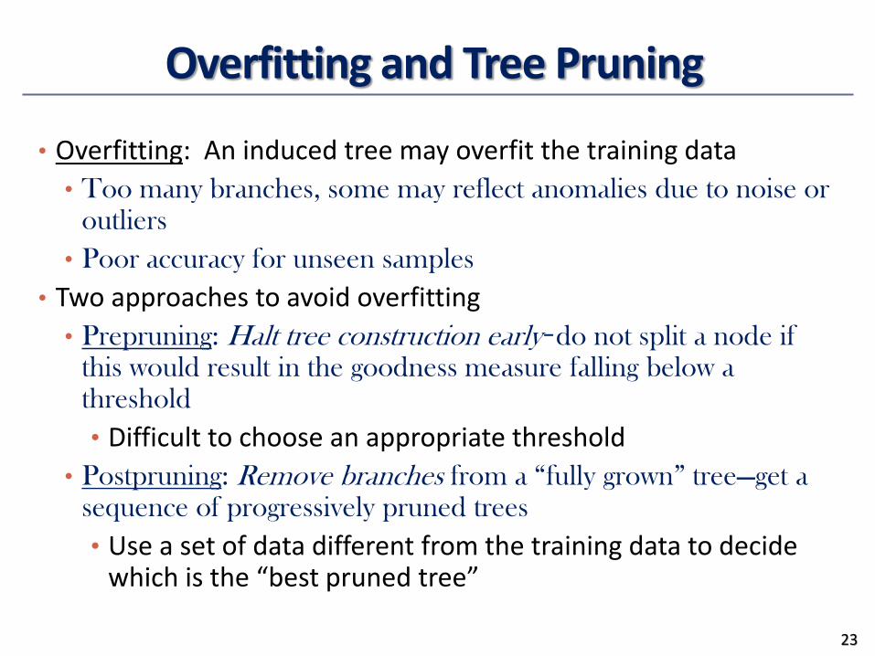
Overfitting and Tree Pruning
• Overfitting: An induced tree may overfit the training data
• Too many branches, some may reflect anomalies due to noise or outliers
• Poor accuracy for unseen samples
• Two approaches to avoid overfitting
• Prepruning: Halt tree construction early ̵ do not split a node if this would result in the goodness measure falling below a threshold
• Difficult to choose an appropriate threshold
• Postpruning: Remove branches from a “fully grown” tree—get a sequence of progressively pruned trees
• Use a set of data different from the training data to decide which is the “best pruned tree”
23
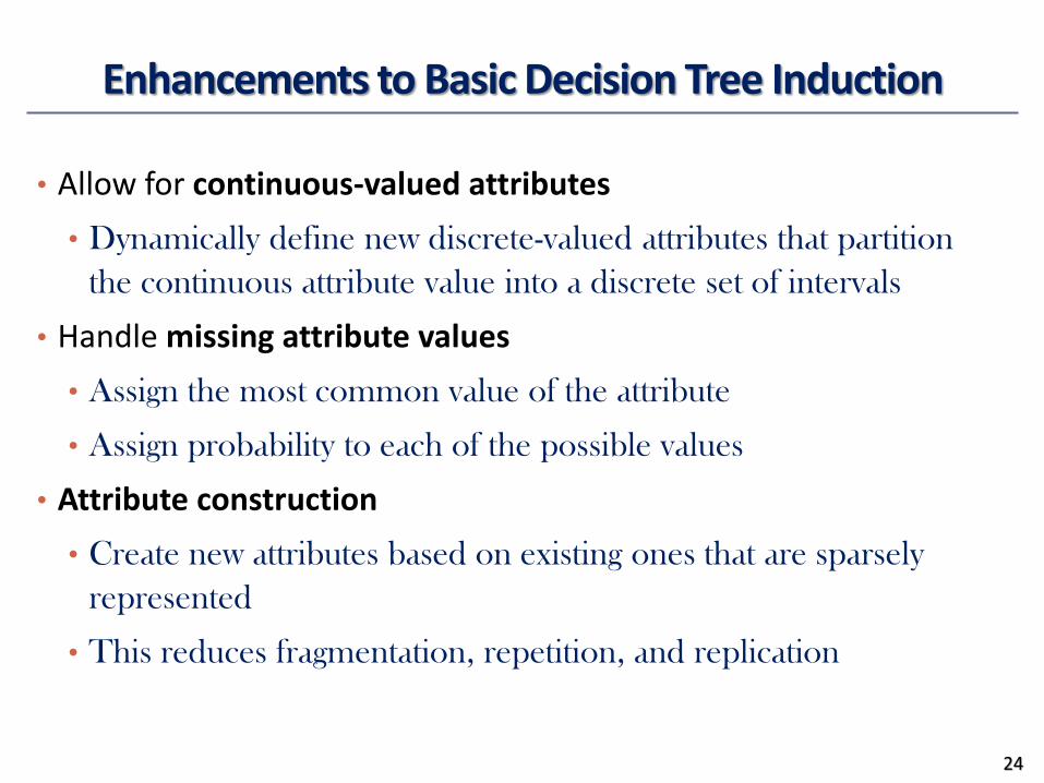
Enhancements to Basic Decision Tree Induction
• Allow for continuous-valued attributes
• Dynamically define new discrete-valued attributes that partition
the continuous attribute value into a discrete set of intervals
• Handle missing attribute values
• Assign the most common value of the attribute
• Assign probability to each of the possible values
• Attribute construction
• Create new attributes based on existing ones that are sparsely
represented
• This reduces fragmentation, repetition, and replication
24
Matrix Data: Classification: Part 1
•Classification: Basic Concepts
•Decision Tree Induction
•Model Evaluation and Selection
• Summary
25

Model Evaluation and Selection
• Evaluation metrics: How can we measure accuracy? Other
metrics to consider?
• Use validation test set of class-labeled tuples instead of
training set when assessing accuracy
• Methods for estimating a classifier’s accuracy:
• Holdout method, random subsampling
• Cross-validation
• Comparing classifiers:
• Confidence intervals
• Cost-benefit analysis and ROC Curves
26
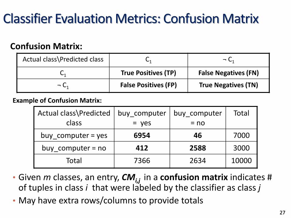
Classifier Evaluation Metrics: Confusion Matrix
Actual class\Predicted class
buy_computer = yes
buy_computer = no
Total
buy_computer = yes 6954 46 7000
buy_computer = no 412 2588 3000
Total 7366 2634 10000
• Given m classes, an entry, CMi,j in a confusion matrix indicates # of tuples in class i that were labeled by the classifier as class j
• May have extra rows/columns to provide totals
Confusion Matrix:
Actual class\Predicted class C1 ¬ C1
C1 True Positives (TP) False Negatives (FN)
¬ C1 False Positives (FP) True Negatives (TN)
Example of Confusion Matrix:
27

Classifier Evaluation Metrics: Accuracy, Error Rate, Sensitivity and Specificity
• Classifier Accuracy, or recognition rate: percentage of test set tuples that are correctly classified
Accuracy = (TP + TN)/All
• Error rate: 1 – accuracy, or
Error rate = (FP + FN)/All
28
Class Imbalance Problem:
One class may be rare, e.g. fraud, or HIV-positive
Significant majority of the negative class and minority of the positive class
Sensitivity: True Positive recognition rate
Sensitivity = TP/P
Specificity: True Negative recognition rate
Specificity = TN/N
A\P C ¬C
C TP FN P
¬C FP TN N
P’ N’ All
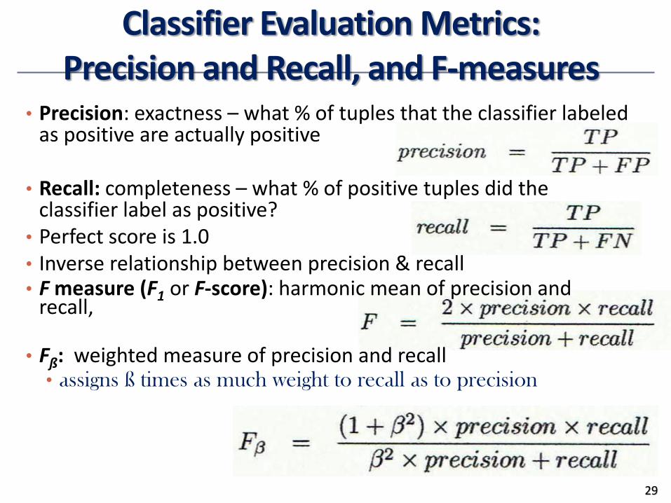
Classifier Evaluation Metrics: Precision and Recall, and F-measures
• Precision: exactness – what % of tuples that the classifier labeled as positive are actually positive
• Recall: completeness – what % of positive tuples did the classifier label as positive?
• Perfect score is 1.0• Inverse relationship between precision & recall• F measure (F1 or F-score): harmonic mean of precision and
recall,
• Fß: weighted measure of precision and recall• assigns ß times as much weight to recall as to precision
29

Classifier Evaluation Metrics: Example
• Precision = 90/230 = 39.13% Recall = 90/300 = 30.00%
Actual Class\Predicted class cancer = yes cancer = no Total Recognition(%)
cancer = yes 90 210 300 30.00 (sensitivity)
cancer = no 140 9560 9700 98.56 (specificity)
Total 230 9770 10000 96.40 (accuracy)
30
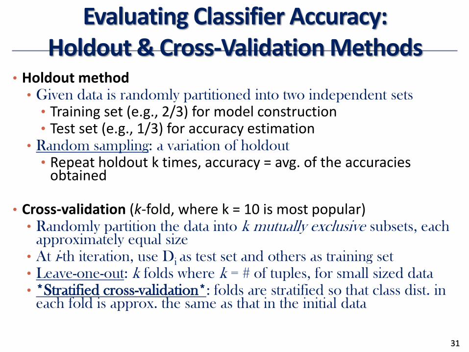
Evaluating Classifier Accuracy:Holdout & Cross-Validation Methods
• Holdout method• Given data is randomly partitioned into two independent sets• Training set (e.g., 2/3) for model construction• Test set (e.g., 1/3) for accuracy estimation
• Random sampling: a variation of holdout• Repeat holdout k times, accuracy = avg. of the accuracies
obtained
• Cross-validation (k-fold, where k = 10 is most popular)• Randomly partition the data into k mutually exclusive subsets, each
approximately equal size• At i-th iteration, use Di as test set and others as training set• Leave-one-out: k folds where k = # of tuples, for small sized data• *Stratified cross-validation*: folds are stratified so that class dist. in
each fold is approx. the same as that in the initial data
31
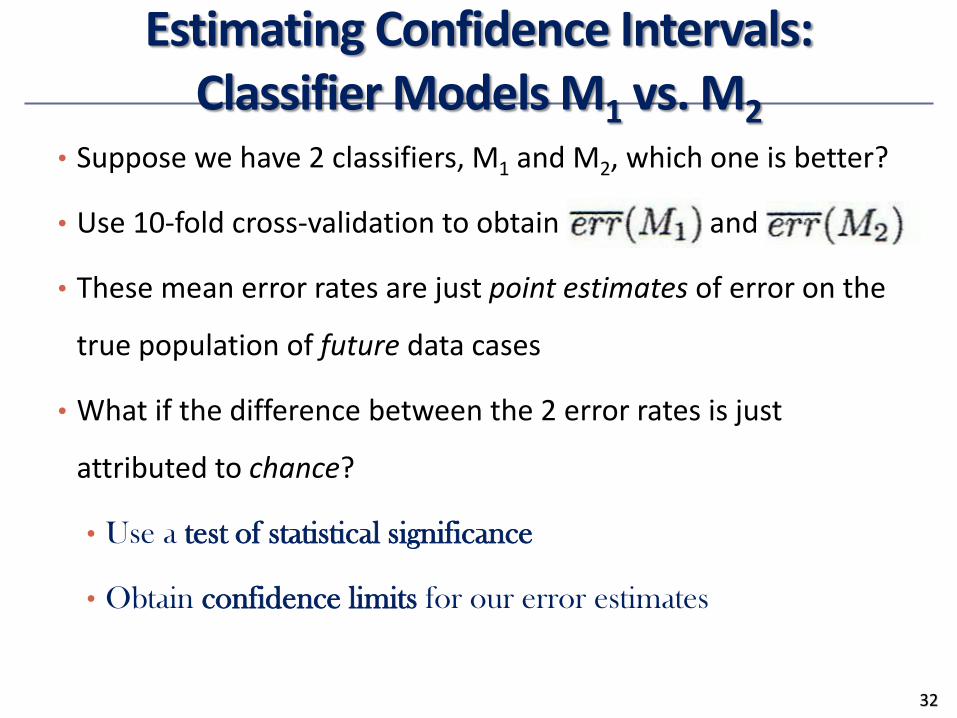
Estimating Confidence Intervals:Classifier Models M1 vs. M2
• Suppose we have 2 classifiers, M1 and M2, which one is better?
• Use 10-fold cross-validation to obtain and
• These mean error rates are just point estimates of error on the
true population of future data cases
• What if the difference between the 2 error rates is just
attributed to chance?
• Use a test of statistical significance
• Obtain confidence limits for our error estimates
32
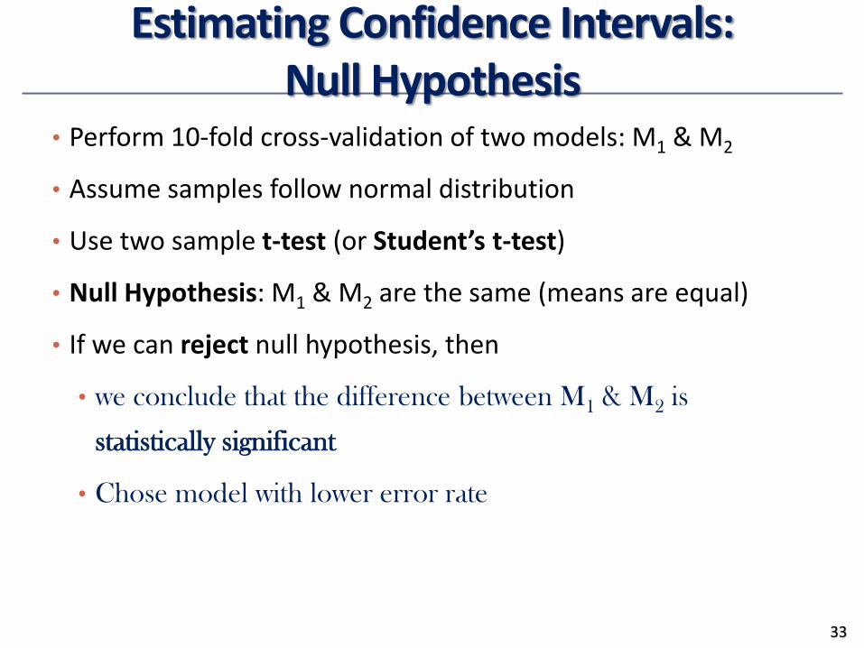
Estimating Confidence Intervals:Null Hypothesis
• Perform 10-fold cross-validation of two models: M1 & M2
• Assume samples follow normal distribution
• Use two sample t-test (or Student’s t-test)
• Null Hypothesis: M1 & M2 are the same (means are equal)
• If we can reject null hypothesis, then
• we conclude that the difference between M1 & M2 is
statistically significant
• Chose model with lower error rate
33

34
Model Selection: ROC Curves
• ROC (Receiver Operating Characteristics) curves: for visual comparison of classification models
• Originated from signal detection theory• Shows the trade-off between the true
positive rate and the false positive rate• The area under the ROC curve is a
measure of the accuracy of the model• Rank the test tuples in decreasing
order: the one that is most likely to belong to the positive class appears at the top of the list
• Area under the curve: the closer to the diagonal line (i.e., the closer the area is to 0.5), the less accurate is the model
Vertical axis represents the true positive rate
Horizontal axis rep. the false positive rate
The plot also shows a diagonal line
A model with perfect accuracy will have an area of 1.0
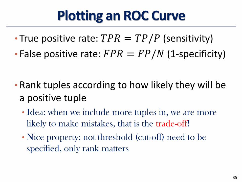
Plotting an ROC Curve
• True positive rate: 𝑇𝑃𝑅 = 𝑇𝑃/𝑃 (sensitivity)
• False positive rate: 𝐹𝑃𝑅 = 𝐹𝑃/𝑁 (1-specificity)
•Rank tuples according to how likely they will be a positive tuple
• Idea: when we include more tuples in, we are more
likely to make mistakes, that is the trade-off!
• Nice property: not threshold (cut-off) need to be
specified, only rank matters
35

36
Example

Issues Affecting Model Selection
• Accuracy
• classifier accuracy: predicting class label
• Speed
• time to construct the model (training time)
• time to use the model (classification/prediction time)
• Robustness: handling noise and missing values
• Scalability: efficiency in disk-resident databases
• Interpretability
• understanding and insight provided by the model
• Other measures, e.g., goodness of rules, such as decision tree size or compactness of classification rules
37

Matrix Data: Classification: Part 1
•Classification: Basic Concepts
•Decision Tree Induction
•Model Evaluation and Selection
• Summary
38
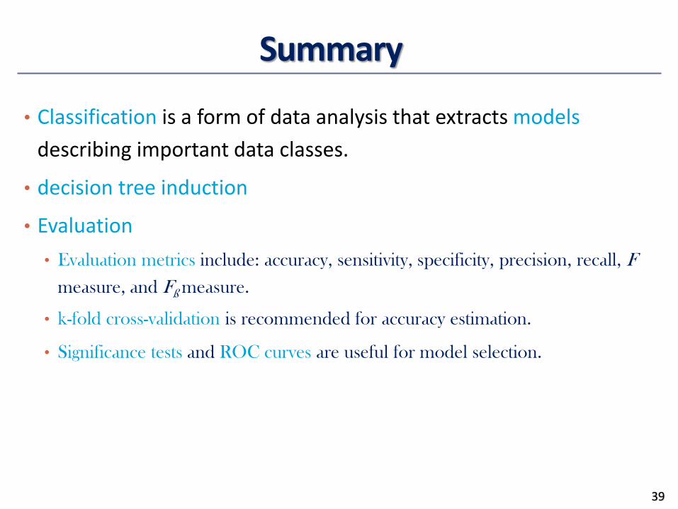
Summary
• Classification is a form of data analysis that extracts models
describing important data classes.
• decision tree induction
• Evaluation
• Evaluation metrics include: accuracy, sensitivity, specificity, precision, recall, F
measure, and Fß measure.
• k-fold cross-validation is recommended for accuracy estimation.
• Significance tests and ROC curves are useful for model selection.
39

•Course project sign-up will be due this Sunday
40
References (1)
• C. Apte and S. Weiss. Data mining with decision trees and decision rules. Future Generation Computer Systems, 13, 1997
• C. M. Bishop, Neural Networks for Pattern Recognition. Oxford University Press, 1995
• L. Breiman, J. Friedman, R. Olshen, and C. Stone. Classification and Regression Trees. Wadsworth International Group, 1984
• C. J. C. Burges. A Tutorial on Support Vector Machines for Pattern Recognition. Data Mining and Knowledge Discovery, 2(2): 121-168, 1998
• P. K. Chan and S. J. Stolfo. Learning arbiter and combiner trees from partitioned data for scaling machine learning. KDD'95
• H. Cheng, X. Yan, J. Han, and C.-W. Hsu, Discriminative Frequent Pattern Analysis for Effective Classification, ICDE'07
• H. Cheng, X. Yan, J. Han, and P. S. Yu, Direct Discriminative Pattern Mining for Effective Classification, ICDE'08
• W. Cohen. Fast effective rule induction. ICML'95
• G. Cong, K.-L. Tan, A. K. H. Tung, and X. Xu. Mining top-k covering rule groups for gene expression data. SIGMOD'05
41

References (2)
• A. J. Dobson. An Introduction to Generalized Linear Models. Chapman & Hall, 1990.
• G. Dong and J. Li. Efficient mining of emerging patterns: Discovering trends and differences. KDD'99.
• R. O. Duda, P. E. Hart, and D. G. Stork. Pattern Classification, 2ed. John Wiley, 2001
• U. M. Fayyad. Branching on attribute values in decision tree generation. AAAI’94.
• Y. Freund and R. E. Schapire. A decision-theoretic generalization of on-line learning and an application to boosting. J. Computer and System Sciences, 1997.
• J. Gehrke, R. Ramakrishnan, and V. Ganti. Rainforest: A framework for fast decision tree construction of large datasets. VLDB’98.
• J. Gehrke, V. Gant, R. Ramakrishnan, and W.-Y. Loh, BOAT -- Optimistic Decision Tree Construction. SIGMOD'99.
• T. Hastie, R. Tibshirani, and J. Friedman. The Elements of Statistical Learning: Data Mining, Inference, and Prediction. Springer-Verlag, 2001.
• D. Heckerman, D. Geiger, and D. M. Chickering. Learning Bayesian networks: The combination of knowledge and statistical data. Machine Learning, 1995.
• W. Li, J. Han, and J. Pei, CMAR: Accurate and Efficient Classification Based on Multiple Class-Association Rules, ICDM'01.
42
References (3)
• T.-S. Lim, W.-Y. Loh, and Y.-S. Shih. A comparison of prediction accuracy, complexity,
and training time of thirty-three old and new classification algorithms. Machine
Learning, 2000.
• J. Magidson. The Chaid approach to segmentation modeling: Chi-squared automatic
interaction detection. In R. P. Bagozzi, editor, Advanced Methods of Marketing
Research, Blackwell Business, 1994.
• M. Mehta, R. Agrawal, and J. Rissanen. SLIQ : A fast scalable classifier for data mining.
EDBT'96.
• T. M. Mitchell. Machine Learning. McGraw Hill, 1997.
• S. K. Murthy, Automatic Construction of Decision Trees from Data: A Multi-Disciplinary
Survey, Data Mining and Knowledge Discovery 2(4): 345-389, 1998
• J. R. Quinlan. Induction of decision trees. Machine Learning, 1:81-106, 1986.
• J. R. Quinlan and R. M. Cameron-Jones. FOIL: A midterm report. ECML’93.
• J. R. Quinlan. C4.5: Programs for Machine Learning. Morgan Kaufmann, 1993.
• J. R. Quinlan. Bagging, boosting, and c4.5. AAAI'96.
43

References (4)
• R. Rastogi and K. Shim. Public: A decision tree classifier that integrates building and pruning. VLDB’98.
• J. Shafer, R. Agrawal, and M. Mehta. SPRINT : A scalable parallel classifier for data mining. VLDB’96.
• J. W. Shavlik and T. G. Dietterich. Readings in Machine Learning. Morgan Kaufmann, 1990.
• P. Tan, M. Steinbach, and V. Kumar. Introduction to Data Mining. Addison Wesley, 2005.
• S. M. Weiss and C. A. Kulikowski. Computer Systems that Learn: Classification and Prediction Methods from Statistics, Neural Nets, Machine Learning, and Expert Systems. Morgan Kaufman, 1991.
• S. M. Weiss and N. Indurkhya. Predictive Data Mining. Morgan Kaufmann, 1997.
• I. H. Witten and E. Frank. Data Mining: Practical Machine Learning Tools and Techniques, 2ed. Morgan Kaufmann, 2005.
• X. Yin and J. Han. CPAR: Classification based on predictive association rules. SDM'03
• H. Yu, J. Yang, and J. Han. Classifying large data sets using SVM with hierarchical clusters. KDD'03.
44


