

Cyberinfrastructure for contaminant source characterization in urban
water distribution systemsSarat Sreepathi, Kumar Mahinthakumar, Ranji Ranjithan,
Downey Brill, Emily ZechmanNorth Carolina State University
Gregor Von LaszewskiUniversity of Chicago
www.secure-water.org
DDDAS Workshop, ICCS 2007, Beijing, ChinaMay 28-31

Our DDDAS Team• North Carolina State University
– Mahinthakumar, Brill, Ranji (PI’s)– Sreepathi, Liu, Jitendra Kumar (Grad Students)– Zechman (Post-Doc)
• University of Chicago– Von Laszewski (PI)
• University of Cincinnati– Uber (PI)– Feng Shang (Post-Doc)
• University of South Carolina– Harrison (PI)
Greater Cincinnati Water Works

Water Distribution Security Problem
Why is this an important problem?
Potentially lethal and public health hazardCause short term chaos and long term issuesDiversionary action to cause service outage
Reduction in fire fighting capacityDistract public & system managers
What needs to be done?
Determine Location of the contaminant source(s)Contamination release history
Identify threat management optionsSections of the network to be shut downFlow controls to
Limit spread of contaminationFlush contamination

DDDAS Project Goal
• Develop an adaptive cyberinfrastructure for threat management in urban water distribution systems– Algorithms– Software– Validation

DDDAS Project Developments (NCSU)
• Problem Aspects• Algorithms• Implementation and Performance

Source Identification Problem
Source Location?
0
1
2
3
4
5
6
7
8
9
10
5 7 9 11 13 15
Time Step (10 mins)
Mas
s Lo
adin
g (g
/min
)
Contaminant Loading Profile?

Source Identification Problem Investigations
• Non-uniqueness– Zechman (WDSA 2006)– Jitendra Kumar (EWRI 2007)– Li Liu (EWRI 2007)
• Binary Sensors– Jitendra Kumar (EWRI 2007)
• Multiple Sources– Jitendra Kumar (EWRI 2007)
• Demand Uncertainty– Venkalaya (MS Thesis 2007)
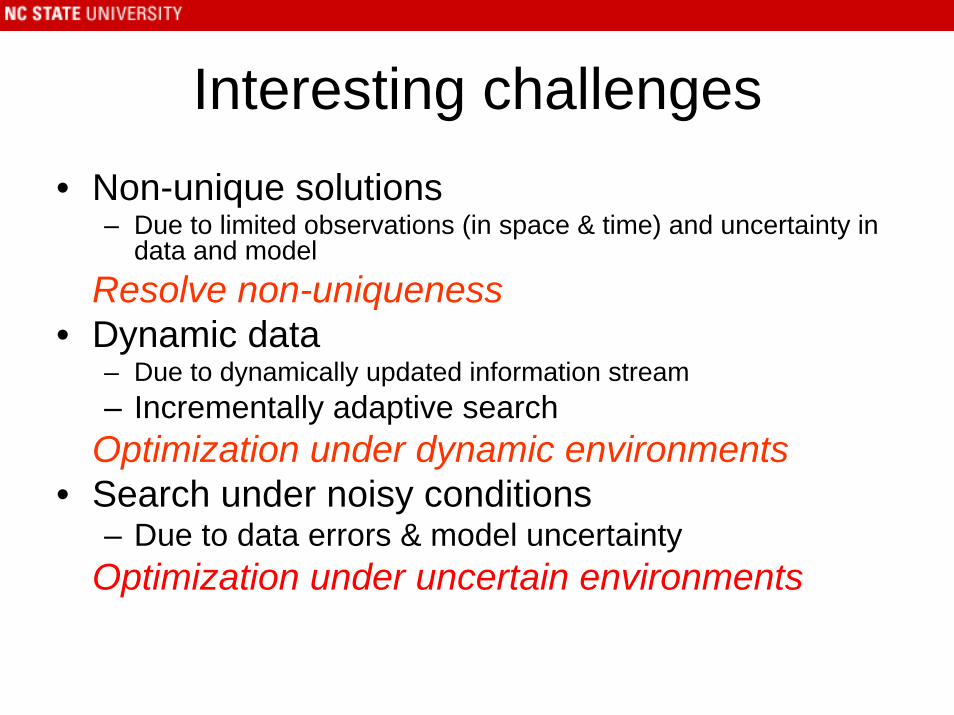
Interesting challenges• Non-unique solutions
– Due to limited observations (in space & time) and uncertainty indata and model
Resolve non-uniqueness• Dynamic data
– Due to dynamically updated information stream– Incrementally adaptive search
Optimization under dynamic environments• Search under noisy conditions
– Due to data errors & model uncertaintyOptimization under uncertain environments

Resolving non-uniqueness
• Underlying premise– In addition to the “optimal” solution, identify
other “good” solutions that fit the observations– Are there different solutions with similar
performance in objective space?Search for alternative solutions

Non-Uniqueness Test Problem
0
1
2
3
4
5
6
7
5 7 9 11 13 15 17
Time Step (10 min) .
Mas
s Lo
adin
g (g
/min
)
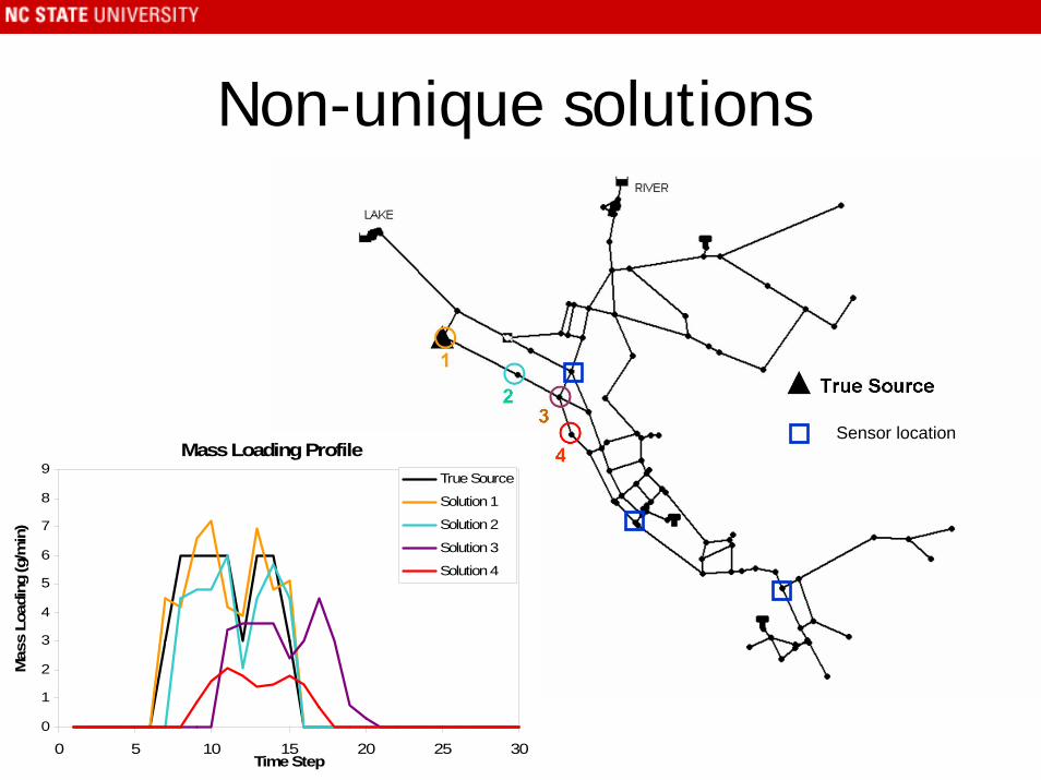
Non-unique solutions
Mass Loading Profile
0
1
2
3
4
5
6
7
8
9
0 5 10 15 20 25 30Time Step
Mas
s Lo
adin
g (g
/min
)
True Source
Solution 1
Solution 2
Solution 3
Solution 4
Sensor location
0
0.1
0.2
0.3
0.4
0.5
0.6
0.7
0.8
0.9
1
1 6 11 16 21 26 31 36 41Time Step
Con
cent
ratio
n (m
g/L)
0
0.1
0.2
0.3
0.4
0.5
0.6
0.7
0.8
0.9
1
1 11 21 31 41Time Step
Con
cent
ratio
n (m
g/L)
0
0.1
0.2
0.3
0.4
0.5
0.6
0.7
0.8
0.9
1
1 11 21 31 41Time Step
Con
cent
ratio
n (m
g/L)
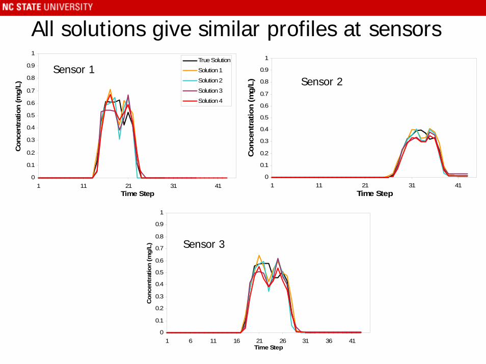
True Solution
Solution 1
Solution 2
Solution 3
Solution 4
Sensor 3
All solutions give similar profiles at sensors
Sensor 1Sensor 2

What can we do about non-uniqueness?
• Incrementally design contamination sampling strategy
• Provide alternatives to decision maker
Non-uniqueness Study Observations
• As expected non-uniqueness increases with the following:– Data errors– Malfunctioning sensors– Low resolution or binary sensors– Decreasing number of sensors– Problem complexity (multiple sources, non-
uniform loading profile)

Algorithmic Developments
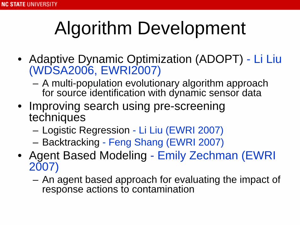
Algorithm Development• Adaptive Dynamic Optimization (ADOPT) - Li Liu
(WDSA2006, EWRI2007)– A multi-population evolutionary algorithm approach
for source identification with dynamic sensor data• Improving search using pre-screening
techniques – Logistic Regression - Li Liu (EWRI 2007)– Backtracking - Feng Shang (EWRI 2007)
• Agent Based Modeling - Emily Zechman (EWRI 2007)– An agent based approach for evaluating the impact of
response actions to contamination

Implementation and Performance
Grid Implementation
• Basic Architecture• Grid Performance Results• Graphical Interface
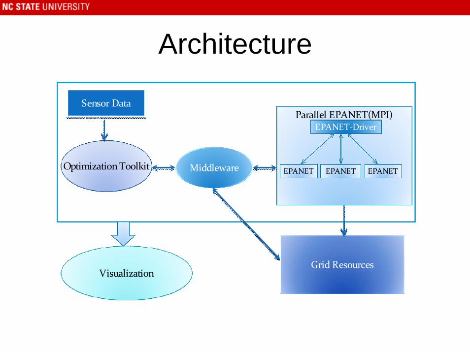
Architecture
Optimization Toolkit
Sensor DataSensor Data
Grid Resources
Parallel EPANET(MPI)EPANET‐Driver
EPANET EPANET EPANETMiddleware
Visualization
Optimization ToolkitOptimization Toolkit
Sensor DataSensor Data
Grid ResourcesGrid Resources
Parallel EPANET(MPI)EPANET‐Driver
EPANET EPANET EPANET
Parallel EPANET(MPI)Parallel EPANET(MPI)EPANET‐DriverEPANET‐Driver
EPANETEPANET EPANETEPANET EPANETEPANETMiddlewareMiddleware
VisualizationVisualization

Simulation Engine - EPANET • Hydraulic and Water Quality modeling tool
for WDS (Water Distribution System)• Developed by EPA (Environmental
Protection Agency)• C language library with a well-defined API

Water Distribution Network Modeling
• Solve for network hydraulics (i.e., pressure, flow)– Depends on
• Water demand/usage• Properties of network components
– Uncertainty/variability– Dynamic system
• Solve for contamination transport– Depends on existing hydraulic conditions– Spatial/temporal variation
• time series of contamination concentration
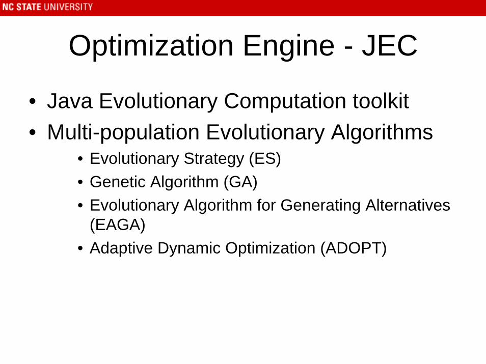
Optimization Engine - JEC
• Java Evolutionary Computation toolkit• Multi-population Evolutionary Algorithms
• Evolutionary Strategy (ES)• Genetic Algorithm (GA)• Evolutionary Algorithm for Generating Alternatives
(EAGA)• Adaptive Dynamic Optimization (ADOPT)

Parallel EPANET Wrapper• Aggregate multiple EPANET simulations• Interoperability with Optimization toolkits
(Java/MATLAB) and middleware• Coarse-grained parallelization• Avoid redundant computations• Maintain persistency in a batch
environment

Wrapper - ParallelizationParallel EPANET(MPI)
EPANET‐Driver
EPANET EPANET EPANET
Persistency in Wrapper• Motivation
–Optimization needs simulations to be computed at every generation
–Significant wait times for invoking simulation code in a batch environment every generation
• Solution–To remain persistent across multiple
generations–Wait time in the job queue only at startup

Python Middleware• Provides seamless interactions between
optimization toolkit and simulation code• Facilitates file based communication• Password-less interface• Invokes job submission script (first time)• Security through public key cryptography• Deployed on Teragrid and SURAgrid• Checks backfill window to appropriately
allocate resources at each site
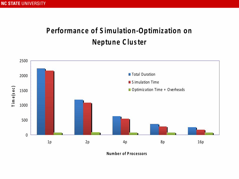
Performance of S imulation‐Optimization on Neptune C lus ter
0
500
1000
1500
2000
2500
1p 2p 4p 8p 16p
Number of P rocessors
Tim
e(se
c)
Total Duration
S imulation Time
Optimiz ation Time + Overheads

Performance of S imulation‐Optimization on Terag ridS imulation module at ANL
Optimization module at NC S A
0
1000
2000
3000
4000
5000
6000
1 2 4 8 16 32 64
Number of P rocessors
Tim
e (s
ec)
Total Time
S imulation Time
Optimiz ation Time
C omm Overhead

Graphical Monitoring Interface
29

water-demo
Performance Optimizations
• Minimizing file system overheads• Eliminating redundant computations• Amortizing queue wait times• Improving processor placements• Multi-threaded visualization

Future Work - Implementation
• Reduce file movement / communication overheads– Asynchronous algorithms to overlap
computation with communication– Improved file transfer protocols– Non-file based communication
• Better resource discovery and allocation mechanisms to minimize queue wait time
• Localizing optimization calculations on remote sites by partitioning algorithms
Challenges
• Resource discovery mechanisms• Asynchronous algorithms• Sampling design

Summary• Algorithmic developments enable use of
dynamic sensor data and identify non-unique solutions
• Source identification problem investigated under a variety of conditions
• Present implementation enables solution of source identification problems by harnessing grid resources – room for improvement..
• Agent based modeling framework enables evaluation of different management scenarios for contamination

Acknowledgements
• This work is supported by National Science Foundation (NSF) under Grant No. CMS-0540316 under the DDDAS program.

Thank you!
Questions?

Backup Slides

Dynamic optimization…
• Underlying premise– Predict solutions using available information
at any time step– Search for a diverse set of solutions (EAGA)– Current solutions are good starting points for
search in the next time step

Adaptive Dynamic Optimization Technique (ADOPT)
• An EA-based multi-population search• Solves as information becomes available
over time• Multiple solutions to assess
non-uniqueness

ADOPT Procedure
Time Step
Time Step t0
t0
Obs
erve
d Co
nc. a
t se
nsor
s
Sub-pop 1
Sub-pop 2Sub-pop 3Sub-pop 4

ADOPT Procedure
Time Step
Conc.
Time Step t1
t1Obs
erve
d Co
nc. a
t se
nsor
s

ADOPT Procedure…
Time Step
Conc.
Obs
erve
d Co
nc. a
t se
nsor
s
Time Step t2
t1 t2

ADOPT Procedure…
Time Step
Conc.
Obs
erve
d Co
nc. a
t se
nsor
s
True source
Time Step t3
t1 t2 t3

Adopt Results for case with Perfect Data
0
0.5
0 10 20 30 40
0
0.5
0 20 40
0
0.5
0 20 40
0
0.5
0 20 40
Node 197 Node 184 Node 211
Node 115
True source
Best solution
Best solution
Prediction Error = 0.026 mg/L
Obs
erve
d Co
nc. (
mg/
L)O
bser
ved
Conc
. (m
g/L)
Time Step (10 mins)

Agent Based Modeling Frameworkfor WDS Contamination Event
Decision Maker Agent
Demand
Public Broadcast
Unusual Water Quality
at Sensors
Change Hydraulics
Water Distribution
System Model
Exposure
Word-of-mouth
Consumer Agents

2:50am
SensorSensor with unusual WQHydrant opened
Number of Sick Consumer Agents
0 - 5 5 - 10
10 - 2020 - 30
> 30
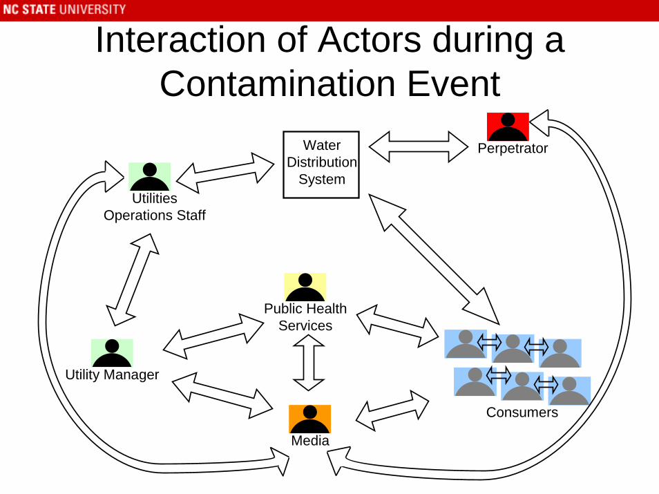
Interaction of Actors during a Contamination Event
Water Distribution
System
Utility Manager
Consumers
Perpetrator
Media
Utilities Operations Staff
Public Health Services
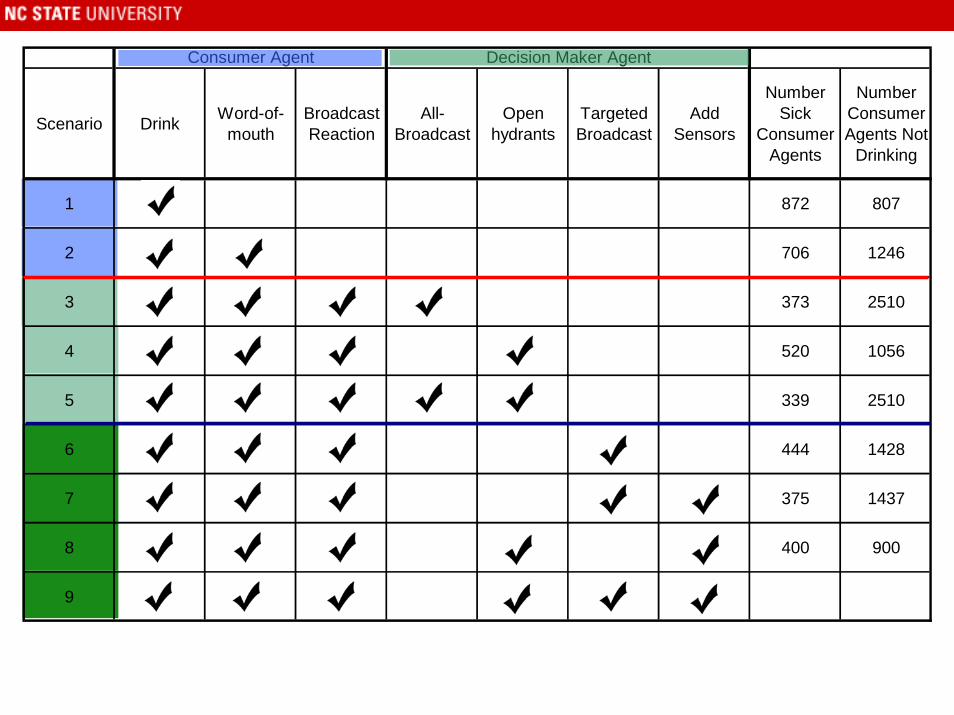
Scenario Drink Word-of-mouth
Broadcast Reaction
All-Broadcast
Open hydrants
Targeted Broadcast
Add Sensors
Number Sick
Consumer Agents
Number Consumer Agents Not
Drinking
1 872 807
2 706 1246
3 373 2510
4 520 1056
5 339 2510
6 444 1428
7 375 1437
8 400 900
9 286 1292
Decision Maker AgentConsumer Agent
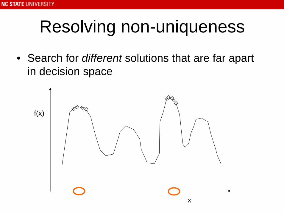
Resolving non-uniqueness
• Search for different solutions that are far apart in decision space
x
f(x)

Resolving non-uniqueness…
• Effects of uncertainty
x
f(x)
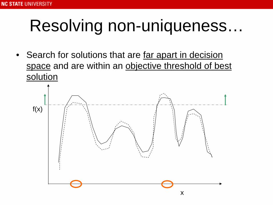
Resolving non-uniqueness…• Search for solutions that are far apart in decision
space and are within an objective threshold of best solution
x
f(x)
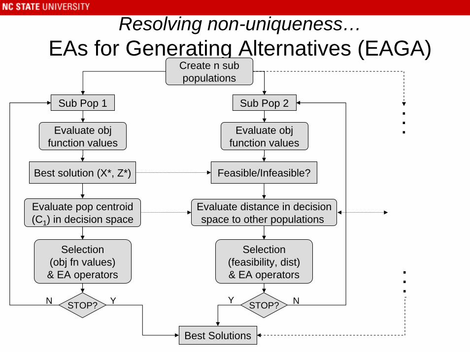
Resolving non-uniqueness…EAs for Generating Alternatives (EAGA)
Create n subpopulations
Sub Pop 1
Evaluate objfunction values
Best solution (X*, Z*)
Evaluate pop centroid(C1) in decision space
Selection(obj fn values)& EA operators
STOP?
Best Solutions
Sub Pop 2
Evaluate objfunction values
Feasible/Infeasible?
Evaluate distance in decisionspace to other populations
Selection(feasibility, dist)& EA operators
STOP?N Y NY
...
...
Binary Sensors
• Sensors that give 0 (no contamination) or 1 (contamination) readings
• Non-uniqueness is more common with these sensors


