

Data driven constraintsfor Gaussian mixtures of factor analyzers:
an application to market segmentation
Francesca Greselin
Francesca Greselin - Universita di Milano-Bicocca,Dipartimento di Statistica e Metodi Quantitativi
Salvatore Ingrassia - Universita di Catania,Dipartimento di Economia e Impresa
November 8, 2013
AG DANK/BCS Meeting 2013 - University College London
Francesca Greselin Market segmentation via mixtures of constrained factor analyzers

Outline
We want to make a first explorative analysis on traffic usage for atelecom company
Mixtures of factor analyzers, estimated through EM
BUT: maximization of the log-likelihood without any constraint isan ill-posed problem (Day, 1969)
to reduce spurious local maximizers and avoid singularities,some authors propose to take a common (diagonal) error matrix(MCFA Baek et al., 2010) or to impose an isotropic error matrix(Bishop and Tippin, 1998)
our proposal: a less constrained approach, based on covariancedecomposition
a first application is shown, suggesting a non-unique behavior ofcustomers inside the traffic plan
Francesca Greselin Market segmentation via mixtures of constrained factor analyzers

Methodology and Aim
Our proposal is to adopt a weakly constrained approach for MLestimation,
having no singularities, and
simultaneously reducing the number of spurious local maxima
Aim
Provide market segmentation for telecom data, by using a latentvariable approach, based on constrained mixtures of gaussian factoranalyzers
Francesca Greselin Market segmentation via mixtures of constrained factor analyzers

The data
A sample of 2072 customers (postpaid plans)with 45 quantitative variables about traffic usage (tot over 6 mths:Aug’12-Jan’13), like
minutes of voice call (Off net, On net, International, to Fixed line)number of events of voice call (Off net, On net, Int, to Fix. l.)number of sent SMS (Off net, On net)number of events of data download from Internetamount of downloaded data (in Kb)minutes of data downloadnumber of events of data download in roaming or GPRSamount of downloaded data in roaming or GPRS (in Kb)minutes of data download in roaming or GPRS
Data is divided into:total / under / over the threshold of the plan / no threshold
Further, we have 10 qualitative variables (ID, age, sex, geographiclocation (2 var), aging as a customer, value, price plan, handset,portability)
Francesca Greselin Market segmentation via mixtures of constrained factor analyzers

One of the (many) open questions in the market
When the market is saturated, the pool of available customers islimited and an operator has to shift from its acquisition strategy toretention because the cost of acquisition is typically five times higherthan retention.
As noted in (Mattersion, 2001)For many telecom executives, figuring out how to deal with Churn isturning out to be the key to very survival of their organizations.
Based on marketing research (Berson et al., 2000), the averagechurn of a wireless operator is about 2% per month. That is, a carrierlooses about a quarter of its customer base each year.
We need a model to understand the data and to devise patterns ofpre-churn customers.
Francesca Greselin Market segmentation via mixtures of constrained factor analyzers

A first step: Exploratory Data Analysis
EDA is an approach to analyzing data sets to summarize their maincharacteristics (Hoaglin et al., 2000), opening some questions in ourminds
what the data can tell us
what assumptions could be reasonably be made w.r.t. the actualdata
what kind of model could be fit
what set of hypotheses could be assessed
. . .
Francesca Greselin Market segmentation via mixtures of constrained factor analyzers

Exploratory Data Analysis
Some questions:
Is the traffic usage highly related to the traffic plan?
Which variables are more related to the customer experience?
Does the plan affect the mean duration of the call? Or the meanamount of download? Or the mean number of SMS?
Is the customer experience influenced by the part of the plan hedoes not exploit?
Is it possible to identify pre-churn customers?
How could the company be aware about new customers needs?
How could the company propose a customer his plan?
Francesca Greselin Market segmentation via mixtures of constrained factor analyzers

Exploratory Data Analysis 1
Tukey promoted the use of a five number summary for quantitativedata:
1 2 3 4 5 6
050
000
1000
0015
0000
2000
0025
0000
(a) Minutes
1 2 3 4 5 6
050
0010
000
1500
0
(b) No. of events
1 2 3 4 5 6
0e+
002e
+07
4e+
076e
+07
8e+
071e
+08
(c) Kbytes
1 2 3 4 5 6
0e+
001e
+07
2e+
073e
+07
4e+
07
(d) Kbytes ExThs
Figure: Summary for Big Internet Home Data, from plan A to FFrancesca Greselin Market segmentation via mixtures of constrained factor analyzers
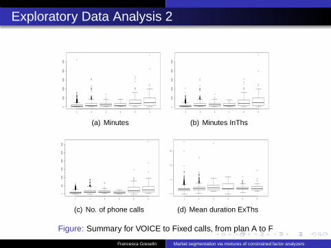
Exploratory Data Analysis 2
1 2 3 4 5 6
010
0020
0030
0040
0050
00
(a) Minutes
1 2 3 4 5 6
010
0020
0030
0040
0050
00
(b) Minutes InThs
1 2 3 4 5 6
050
010
0015
0020
0025
0030
00
(c) No. of phone calls
1 2 3 4 5 6
05
1015
(d) Mean duration ExThs
Figure: Summary for VOICE to Fixed calls, from plan A to F
Francesca Greselin Market segmentation via mixtures of constrained factor analyzers

Exploratory Data Analysis 3
1 2 3 4 5 6
010
0020
0030
0040
00
(a) No. of SMS Off net
1 2 3 4 5 6
050
010
0015
0020
0025
0030
00
(b) No. of SMS Off net InT
1 2 3 4 5 6
010
0020
0030
0040
0050
0060
00
(c) No. of SMS On net
1 2 3 4 5 6
010
0020
0030
0040
0050
00
(d) No. of SMS On net InT
Figure: Summary for number of SMS sent Off (upper row) and On Net(lower), from plan A to F Francesca Greselin Market segmentation via mixtures of constrained factor analyzers

Exploratory Data Analysis 4
How is the ”number of phone calls” variable distributed into thedifferent plans?
#ev Voice On Plan A
x
Den
sity
0 500 1000 1500 2000
0.00
000.
0010
0.00
20
#ev InT Voice On Plan A
x
Den
sity
0 500 1000 15000.
000
0.00
20.
004
#ev Voice On Plan B
x
Den
sity
0 500 1000 2000
0.00
000.
0010
0.00
20
#ev InT Voice On Plan B
x
Den
sity
0 500 1000 1500 2000
0.00
000.
0010
0.00
200.
0030
#ev Voice Off Plan A
x
Den
sity
0 500 1000 1500 2000
0.00
000.
0005
0.00
100.
0015
#ev InT Voice Off Plan A
x
Den
sity
0 500 1000 1500 2000
0.00
000.
0005
0.00
100.
0015
#ev Voice Off Plan B
x
Den
sity
0 500 1000 2000
0.00
000.
0004
0.00
080.
0012
#ev InT Voice Off Plan B
x
Den
sity
0 500 1000 2000
0.00
000.
0005
0.00
100.
0015
Figure: No. of phone calls On and Off Net - plan A (left) and B (right)
Francesca Greselin Market segmentation via mixtures of constrained factor analyzers
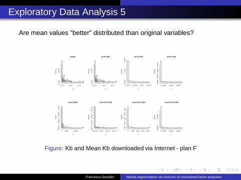
Exploratory Data Analysis 5
Are mean values ”better” distributed than original variables?
kb BIH
x
Den
sity
0e+00 4e+07 8e+07
0.0e
+00
1.0e
−07
kb InT BIH
xD
ensi
ty
0e+00 4e+07 8e+07
0.0e
+00
1.0e
−07
kb ExT BIH
x
Den
sity
0.0e+00 5.0e+06 1.0e+07 1.5e+07
0.0e
+00
1.0e
−06
2.0e
−06
kb NoT BIH
x
Den
sity
0 50000 150000 250000
0.00
000
0.00
005
0.00
010
0.00
015
mean kbBIH
x
Den
sity
0 50000 150000
0.00
000
0.00
004
0.00
008
0.00
012
mean kb InT BIH
x
Den
sity
0.0e+00 1.0e+07 2.0e+07 3.0e+07
0.0e
+00
4.0e
−07
8.0e
−07
1.2e
−06
mean kb ExT BIH
x
Den
sity
0 2000 4000 6000 8000
0.00
00.
001
0.00
20.
003
0.00
4
mean kb NoT BIH
x
Den
sity
0 50000 150000 250000
0.00
000
0.00
010
Figure: Kb and Mean Kb downloaded via Internet - plan F
Francesca Greselin Market segmentation via mixtures of constrained factor analyzers
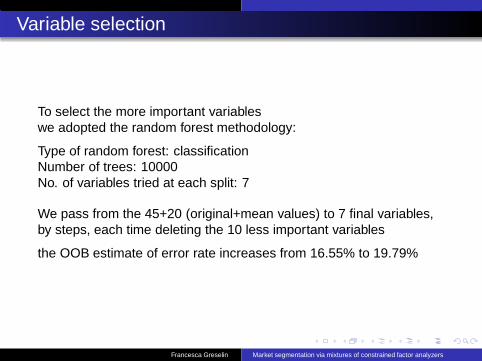
Variable selection
To select the more important variableswe adopted the random forest methodology:
Type of random forest: classificationNumber of trees: 10000No. of variables tried at each split: 7
We pass from the 45+20 (original+mean values) to 7 final variables,by steps, each time deleting the 10 less important variables
the OOB estimate of error rate increases from 16.55% to 19.79%
Francesca Greselin Market segmentation via mixtures of constrained factor analyzers

The 7 selected variables
Kb BIH
ev SMS On
evSMS Off
min Voice to Fixed
min InT Voice to Fixed
min Voice Off net
min Voice On net
Francesca Greselin Market segmentation via mixtures of constrained factor analyzers
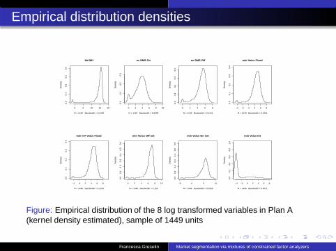
Empirical distribution densities
0 5 10 15 20
0.0
0.1
0.2
0.3
0.4
kb BIH
N = 1449 Bandwidth = 0.2469
Den
sity
0 2 4 6 8 10
0.0
0.1
0.2
0.3
ev SMS On
N = 1449 Bandwidth = 0.3099D
ensi
ty
0 2 4 6 8
0.0
0.1
0.2
0.3
0.4
ev SMS Off
N = 1449 Bandwidth = 0.2141
Den
sity
−2 0 2 4 6 8
0.0
0.1
0.2
0.3
0.4
min Voice Fixed
N = 1449 Bandwidth = 0.2401
Den
sity
−2 0 2 4 6 8
0.0
0.1
0.2
0.3
0.4
min InT Voice Fixed
N = 1449 Bandwidth = 0.2375
Den
sity
0 2 4 6 8 10
0.0
0.1
0.2
0.3
0.4
0.5
0.6
min Voice Off net
N = 1449 Bandwidth = 0.155
Den
sity
−5 0 5 10
0.0
0.1
0.2
0.3
0.4
0.5
0.6
min Voice On net
N = 1449 Bandwidth = 0.2659
Den
sity
−4 −2 0 2 4 6 8
0.0
0.2
0.4
0.6
0.8
1.0
min Voice Int
N = 1449 Bandwidth = 0.4571
Den
sity
Figure: Empirical distribution of the 8 log transformed variables in Plan A(kernel density estimated), sample of 1449 units
Francesca Greselin Market segmentation via mixtures of constrained factor analyzers

Empirical distribution densities
0 5 10 15 20
0.0
0.1
0.2
0.3
0.4
kb BIH
N = 442 Bandwidth = 0.3781
Den
sity
0 2 4 6 8 10
0.0
0.1
0.2
0.3
ev SMS On
N = 442 Bandwidth = 0.3486D
ensi
ty
0 2 4 6 8
0.0
0.1
0.2
0.3
0.4
ev SMS Off
N = 442 Bandwidth = 0.2469
Den
sity
−2 0 2 4 6 8
0.0
0.1
0.2
0.3
0.4
min Voice Fixed
N = 442 Bandwidth = 0.2889
Den
sity
−2 0 2 4 6 8
0.0
0.1
0.2
0.3
0.4
min InT Voice Fixed
N = 442 Bandwidth = 0.2953
Den
sity
0 2 4 6 8 10
0.0
0.1
0.2
0.3
0.4
0.5
0.6
min Voice Off net
N = 442 Bandwidth = 0.2025
Den
sity
−5 0 5 10
0.0
0.1
0.2
0.3
0.4
0.5
0.6
min Voice On net
N = 442 Bandwidth = 0.3081
Den
sity
−4 −2 0 2 4 6 8
0.0
0.2
0.4
0.6
0.8
1.0
min Voice Int
N = 442 Bandwidth = 0.2873
Den
sity
Figure: Empirical distribution of the 8 log transformed variables in Plan B(kernel density estimated), sample of 442 units
Francesca Greselin Market segmentation via mixtures of constrained factor analyzers

Empirical distribution densities
0 5 10 15 20
0.0
0.1
0.2
0.3
0.4
kb BIH
N = 31 Bandwidth = 1.108
Den
sity
0 2 4 6 8 10
0.0
0.1
0.2
0.3
ev SMS On
N = 31 Bandwidth = 0.9123D
ensi
ty
0 2 4 6 8
0.0
0.1
0.2
0.3
0.4
ev SMS Off
N = 31 Bandwidth = 0.6114
Den
sity
−2 0 2 4 6 8
0.0
0.1
0.2
0.3
0.4
min Voice Fixed
N = 31 Bandwidth = 0.3925
Den
sity
−2 0 2 4 6 8
0.0
0.1
0.2
0.3
0.4
min InT Voice Fixed
N = 31 Bandwidth = 0.4274
Den
sity
0 2 4 6 8 10
0.0
0.1
0.2
0.3
0.4
0.5
0.6
min Voice Off net
N = 31 Bandwidth = 0.3106
Den
sity
−5 0 5 10
0.0
0.1
0.2
0.3
0.4
0.5
0.6
min Voice On net
N = 31 Bandwidth = 0.6063
Den
sity
−4 −2 0 2 4 6 8
0.0
0.2
0.4
0.6
0.8
1.0
min Voice Int
N = 31 Bandwidth = 1.664
Den
sity
Figure: Empirical distribution of the 8 log transformed variables in Plan C(kernel density estimated), sample of 31 units
Francesca Greselin Market segmentation via mixtures of constrained factor analyzers
Empirical distribution densities
0 5 10 15 20
0.0
0.1
0.2
0.3
0.4
kb BIH
N = 8 Bandwidth = 1.287
Den
sity
0 2 4 6 8 10
0.0
0.1
0.2
0.3
ev SMS On
N = 8 Bandwidth = 0.5995D
ensi
ty
0 2 4 6 8
0.0
0.1
0.2
0.3
0.4
ev SMS Off
N = 8 Bandwidth = 0.5498
Den
sity
−2 0 2 4 6 8
0.0
0.1
0.2
0.3
0.4
min Voice Fixed
N = 8 Bandwidth = 0.6016
Den
sity
−2 0 2 4 6 8
0.0
0.1
0.2
0.3
0.4
min InT Voice Fixed
N = 8 Bandwidth = 0.5968
Den
sity
0 2 4 6 8 10
0.0
0.1
0.2
0.3
0.4
0.5
0.6
min Voice Off net
N = 8 Bandwidth = 0.7696
Den
sity
−5 0 5 10
0.0
0.1
0.2
0.3
0.4
0.5
0.6
min Voice On net
N = 8 Bandwidth = 0.3816
Den
sity
−4 −2 0 2 4 6 8
0.0
0.2
0.4
0.6
0.8
1.0
min Voice Int
N = 8 Bandwidth = 1.869
Den
sity
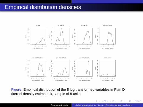
Figure: Empirical distribution of the 8 log transformed variables in Plan D(kernel density estimated), sample of 8 units
Francesca Greselin Market segmentation via mixtures of constrained factor analyzers
Empirical distribution densities
0 5 10 15 20
0.0
0.1
0.2
0.3
0.4
kb BIH
N = 88 Bandwidth = 0.847
Den
sity
0 2 4 6 8 10
0.0
0.1
0.2
0.3
ev SMS On
N = 88 Bandwidth = 0.4103D
ensi
ty
0 2 4 6 8
0.0
0.1
0.2
0.3
0.4
ev SMS Off
N = 88 Bandwidth = 0.3546
Den
sity
−2 0 2 4 6 8
0.0
0.1
0.2
0.3
0.4
min Voice Fixed
N = 88 Bandwidth = 0.3876
Den
sity
−2 0 2 4 6 8
0.0
0.1
0.2
0.3
0.4
min InT Voice Fixed
N = 88 Bandwidth = 0.387
Den
sity
0 2 4 6 8 10
0.0
0.1
0.2
0.3
0.4
0.5
0.6
min Voice Off net
N = 88 Bandwidth = 0.2487
Den
sity
−5 0 5 10
0.0
0.1
0.2
0.3
0.4
0.5
0.6
min Voice On net
N = 88 Bandwidth = 0.3526
Den
sity
−4 −2 0 2 4 6 8
0.0
0.2
0.4
0.6
0.8
1.0
min Voice Int
N = 88 Bandwidth = 0.9976
Den
sity
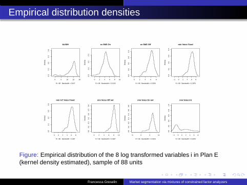
Figure: Empirical distribution of the 8 log transformed variables i in Plan E(kernel density estimated), sample of 88 units
Francesca Greselin Market segmentation via mixtures of constrained factor analyzers

Empirical distribution densities
0 5 10 15 20
0.0
0.1
0.2
0.3
0.4
kb BIH
N = 54 Bandwidth = 0.6358
Den
sity
0 2 4 6 8 10
0.0
0.1
0.2
0.3
ev SMS On
N = 54 Bandwidth = 0.6336D
ensi
ty
0 2 4 6 8
0.0
0.1
0.2
0.3
0.4
ev SMS Off
N = 54 Bandwidth = 0.6382
Den
sity
−2 0 2 4 6 8
0.0
0.1
0.2
0.3
0.4
min Voice Fixed
N = 54 Bandwidth = 0.4797
Den
sity
−2 0 2 4 6 8
0.0
0.1
0.2
0.3
0.4
min InT Voice Fixed
N = 54 Bandwidth = 0.4797
Den
sity
0 2 4 6 8 10
0.0
0.1
0.2
0.3
0.4
0.5
0.6
min Voice Off net
N = 54 Bandwidth = 0.3082
Den
sity
−5 0 5 10
0.0
0.1
0.2
0.3
0.4
0.5
0.6
min Voice On net
N = 54 Bandwidth = 0.4458
Den
sity
−4 −2 0 2 4 6 8
0.0
0.2
0.4
0.6
0.8
1.0
min Voice Int
N = 54 Bandwidth = 1.215
Den
sity
Figure: Empirical distribution of the 8 log transformed variables in Plan F(kernel density estimated), sample of 54 units
Francesca Greselin Market segmentation via mixtures of constrained factor analyzers

Mixture of Gaussian Factor Analyzers
Let f (x; θ) be the density of the d-dimensional random variable X
f (x; θ) =G∑
g=1
πgφd (x;µg,Σg)
MGFA explain the correlation between a set of d variables in terms ofa lower number q of underlying factors:
Xi = µg + ΛgUig + eig with prob πg for i = 1, . . . , n, g = 1, . . . ,G
whereΛg is a d × q matrix of factor loadings,U1g , . . . ,Ung ∼ N (0, Iq) are the factors, ind. w.r.t. eig,eig ∼ N (0,Ψg) are the errors with Ψg d × d diagonal matrix.
Francesca Greselin Market segmentation via mixtures of constrained factor analyzers

Mixture of Gaussian Factor Analyzers
Under these assumptions,
Σg = ΛgΛ′g +Ψg, d(q + 1) params.
and the parameter vector is
θGMFA(d , q,G) = µg,Λg,Ψg , πg(g = 1, . . . ,G − 1)
Francesca Greselin Market segmentation via mixtures of constrained factor analyzers

The EM algorithm for MGFA
Given an initial random clustering z(0), on the (k + 1)− th iteration,
1 Compute z(k+1)ig and consequently obtain π(k+1)
g and µ(k+1)g and
also n(k+1)g and S(k+1)
g in the usual way;
2 Set a starting value for Λg and Ψg from S(k+1)g ;
3 Iterate the following steps, until convergence on Λg and Ψg :1 γg ← γ
+g = Λ
′
g(ΛgΛ′
g +Ψg)−1 and
Θg ← Θ+g = Iq − γgΛg + γgS(k+1)
g γ′
g ;2 Λg ← Λ
+g = S(k+1)
g γ′
g(Θ−1g ) and
Ψg ← Ψ+g = diag
S(k+1)g − Λ
+g γgS(k+1)
g
;
4 Compute Σg = ΛgΛ′g +Ψg and evaluate the log-likelihood, to
check for convergence.
Francesca Greselin Market segmentation via mixtures of constrained factor analyzers

ML in constrained parametric spaces
The maximization of L over θGMFA(d , q,G) is an ill-posed problem.Further, a number of spurious maximizers could arise.
Hathaway (1985) proposed a constrained ML: Let c ∈ (0, 1], then thefollowing constraints
min1≤h 6=j≤k
λ(ΣhΣ−1j ) ≥ c (1)
on the eigenvalues λ of ΣhΣ−1j leads to properly defined,
scale-equivariant, consistent ML-estimators for the mixture-of-normalcase.
Francesca Greselin Market segmentation via mixtures of constrained factor analyzers

ML in constrained parametric spaces
To assure (1) we can impose the stronger condition
a ≤ λig ≤ b, i = 1, . . . , d ; g = 1, . . . ,G (2)
where λig = λi(Σg), and a, b ∈ R+: a/b ≥ c, see Ingrassia (2004).
Due to the structure of the covariance matrix Σg , (2) translates into
a ≤ λig(ΛgΛ′g +Ψg) ≤ b
Francesca Greselin Market segmentation via mixtures of constrained factor analyzers

ML in constrained parametric spaces
Finally, we set
d2ig + ψig ≥ a i = 1, . . . , d (3)
dig ≤√
b − ψig i = 1, . . . , q (4)
ψig ≤ b i = q + 1, . . . , d (5)
for g = 1, . . . ,G, where dig denote the singular values of Λg
and ψig denote the eigenvalues of Ψg.
In particular, (3) reduces to ψig ≥ a for i = (q + 1), . . . , d .
Francesca Greselin Market segmentation via mixtures of constrained factor analyzers

How do we choose constraints?
If we do not have any a priori information on a, b, or c, choosing theconstrained parameter space is a difficult issue.
The constant c can be chosen by computing the profile L(c), forsome set of grid points c ∈ (0, 1] (Yao, 2010)
Rocci (2012) compute c by cross validation.
Both methods are computationally intensive.
We expect that the constrained algorithm, run with different values ofthe bounds, can give us a hint on how to choose them properly, byobserving the final L(c).Optimal values of the bounds should correspond to some agreement,over different random starts, on optimal values of L(c). Conversely, asimultaneous drop in L(c) observed for a new bound, over differentrandom starts, indicates that the new constraint is too strong for thedata at hand.
Francesca Greselin Market segmentation via mixtures of constrained factor analyzers

Data-driven upper bound
Procedure: Choice of the upper bound b
1 compute Cov(S) of sample S and set λ∗ = λmax(Cov(S));2 choose an integer m and set b = (b1, . . . , bm) ∈ R
m where
bj =j
mλ∗ for j = 1, . . . , (m − 1) bm = +∞;
3 for j = m, m − 1 run the unconstrained EM algorithm with b = bj and evaluate Lj ;
4 while j > 1 and Lj ≥ Lj+1:- decrease j ;- run the constrained EM algorithm with b = bj and evaluate Lj ;
5 set b = bj−1 and θ = argθ
max Lj−1(θ).
An analogous procedure can be devised for the lower bound, after setting λ∗ = λmin(Cov(S)), for
more details see Greselin and Ingrassia (2013).
Francesca Greselin Market segmentation via mixtures of constrained factor analyzers

Mixtures of Factor Analyzers with Common FactorLoadings
We want to compare our proposal with the well known MCFA model.The latter is a recent method to deal with ”constrained” maximizationfor EM, which at the same time allows for greater reduction in thenumber of parameters. The authors add the two following constraints(Baek et al., 2010)
µg = Aξg
andΣg = AΩgA′ + D
Francesca Greselin Market segmentation via mixtures of constrained factor analyzers

Application: How is traffic usage in Plan A?
Table: Results of constrained GMFA on Plan A (69.93% of customers) for d = 7, q = 4,G = 2
run No iter L0 Lfin BIC α1 α20 71 -12337.53 -11404.84 23428.37 0.6541167 0.34588331 60 -13843.82 -11404.85 23428.39 0.6541363 0.34586372 16 -13726.44 -10859.68 22338.05 0.7537929 0.24620713 34 -13681.53 -10859.69 22338.06 0.7537701 0.24622994 59 -13716.74 -11404.85 23428.38 0.6541293 0.34587075 53 -13926.21 -11404.85 23428.38 0.6541314 0.34586866 41 -13712.32 -11404.85 23428.38 0.3458635 0.65413657 7 -13839.80 -11594.34 23807.36 0.7654098 0.23459028 39 -13810.36 -10859.69 22338.06 0.2462301 0.75376999 30 -13824.78 -10859.69 22338.07 0.2462284 0.7537716
10 40 -13948.37 -10859.69 22338.06 0.7537700 0.246230011 34 -13493.07 -10859.69 22338.07 0.2462288 0.753771212 35 -13714.11 -11112.42 22843.51 0.7260618 0.273938213 35 -13864.51 -10859.69 22338.06 0.2462299 0.753770114 34 -13827.36 -10859.69 22338.06 0.2462297 0.753770315 54 -13802.20 -11404.84 23428.37 0.6541133 0.345886716 28 -13686.70 -11588.50 23795.69 0.7827988 0.217201217 45 -13862.32 -10859.69 22338.06 0.2462295 0.753770518 35 -13697.06 -10859.69 22338.07 0.2462280 0.753772019 34 -13883.69 -10859.69 22338.07 0.7537716 0.246228420 21 -13788.65 -11394.43 23407.55 0.3971774 0.6028226
Table: Vector b of values for the upper bound in constrained ML λ∗ = 11.56587
2.313174 4.626348 6.939522 9.252696 11.56587 ∞
Francesca Greselin Market segmentation via mixtures of constrained factor analyzers

Application: How is traffic usage in Plan A?
Table: Results of MCFA on Plan A (max 50 iter, max 50 init)
d Lfin BIC2 -13664 275323 -12917 261114 -12573 254965 -12684 247896 -12666 24828
where BIC= −2 logLfin − k log(n),n is the sample size and k is the number of estimated parameters.
The Bayesian information criterion (BIC) is a criterion for modelselection among a finite set of models, based in a penalizedlog-likelihood. The best model is the one with lower BIC.
Francesca Greselin Market segmentation via mixtures of constrained factor analyzers

Conclusions
Aiming at modeling traffic usage, we have employed mixtures ofgaussian factors analyzers.
To face the estimation issues, we considered a constrained approach,where the bounds can be obtained by a data-driven method.
We compared our results to the well known MCFA approach on thelargest subsample of customers.
First results reveal at least two different behaviors among thecustomers, even inside the same plan.
Francesca Greselin Market segmentation via mixtures of constrained factor analyzers

References
Baek, J., McLachlan, G., and Flack, L. (2010). Mixtures of factor analyzers with common factorloadings: Applications to the clustering and visualization of high-dimensional data. PatternAnalysis and Machine Intelligence, IEEE Transactions on, 32(7), 1298 –1309.
Berson, A., Smith, S., and Thearling, K. (2000). Building data mining applications for crm. NewYork.
Bishop, C. M. and Tippin, M. E. (1998). A hierarchical latent variable model for data visualization.IEEE Transactions on Pattern analysis and Machine Intelligence, 20, 281–293.
Day, N. (1969). Estimating the components of a mixture of normal distributions. Biometrika, 56(3),463–474.
Greselin, F. and Ingrassia, S. (2013). Maximum likelihood estimation in constrained parameterspaces for mixtures of factor analyzers. Statistics and Computing, DOI:10.1007/s11222-013-9427-z, forthcoming.
Hathaway, R. (1985). A constrained formulation of maximum-likelihood estimation for normalmixture distributions. The Annals of Statistics, 13(2), 795–800.
Hoaglin, D. C., Mosteller, F., and Tuckey, J. W. (2000). Understanding Robust and Exploratory DataAnalysis. Wiley Classic Library Edition, NewYork.
Ingrassia, S. (2004). A likelihood-based constrained algorithm for multivariate normal mixturemodels. Statistical Methods & Applications, 13, 151–166.
Mattersion, R. (2001). Telecom Churn Management. APDG Publishing, Fuquay-Varina, NC.
Rocci, R. (2012). Gaussian mixture models: constrained and penalized approaches. In MBC2
Workshop, Catania (Italy).
Yao, W. (2010). A profile likelihood method for normal mixture with unequal variance. Journal ofStatistical Planning and Inference, 140(7), 2089 – 2098.
Francesca Greselin Market segmentation via mixtures of constrained factor analyzers


![ONLINE KERNEL LEARNING FOR INTERACTIVE RETRIEVAL IN ...people.rennes.inria.fr/Philippe.Gosselin/pdf/gosselin12icip.pdf · sual dictionary using for instance K-means, Gaussian Mixtures[1]](https://static.documents.pub/doc/80x56/602c55ab6db38f500951d53e/online-kernel-learning-for-interactive-retrieval-in-sual-dictionary-using-for.jpg)


