

Defects Classification of Laser Metal Deposition Using Acoustic Emission Sensor
Haythem Gaja*, Frank Liou*+ * Mechanical Engineering Missouri University of Science and Technology, Rolla, MO 65409
Abstract
Laser metal deposition (LMD) is an advanced additive manufacturing (AM) process used
to build or repair metal parts layer by layer for a range of different applications. Any presence of
deposition defects in the part produced causes change in the mechanical properties and might
cause failure to the part. In this work, defects monitoring system was proposed to detect and
classify defects in real time using an acoustic emission (AE) sensor and an unsupervised pattern
recognition analysis. Time domain and frequency domain, and relevant descriptors were used in
the classification process to improve the characterization and the discrimination of the defects
sources. The methodology was found to be efficient in distinguishing two types of signals that
represent two kinds of defects. A cluster analysis of AE data is achieved and the resulting
clusters correlated with the defects sources during laser metal deposition.
Keywords: Laser metal deposition, Acoustic emission, Deposition defects, Clustering analysis
INTRODUCTION
In general additive manufacturing is extensively used even though monitoring and
detection of defects during AM still require a better understanding. One of the difficulties in
using an adaptive control and LMD monitoring system is the accurate detection of defects as
being formed during the metal deposition. The objective of monitoring laser metal deposition
process is to prevent and detect damage of produced part for any deposition path and part design.
In the LMD process, particular changes in the acoustic emission signal indicate the present of
defects, these changes must be carefully considered to ensure the effectiveness of the control
system. AE has the advantage of real-time, continuous monitoring of LMD. The central goal of
such a system is to indicate the occurrence of defects events, but classifying the type of defect is
also necessary for the better use of the system and suggestion of corrective remedies.
Bohemen [1] demonstrated that martensite formation during gas tungsten arc (GTA)
welding of steel 42CrMo4 can be monitored by means of AE. It was shown that a particular
relation exists between the root mean square (RMS) value of the measured AE and the volume
rate of the martensite formation during GTA welding. Grad et al. [2] examined the acoustic
waves generated during short circuit gas metal arc welding process. It was found that the
acoustic method could be used to assess welding process stability and to detect the severe
discrepancies in arc behavior.
Yang [3] used an Acoustic emission (AE) sensor to identify damage detection in metallic
materials. Results suggested a strong correlation between AE features, i.e., RMS value of the
1952
Solid Freeform Fabrication 2017: Proceedings of the 28th Annual InternationalSolid Freeform Fabrication Symposium – An Additive Manufacturing Conference

reconstructed acoustic emission signal, and surface burn, residual stress value, as well as
hardness of steels. Diego-Vallejo [4] in his work found that the focus position, as an important
parameter in the laser material interactions, changes the dynamics and geometric profile of the
machined surface and the statistical properties of measured AE signal.
Recently, Siracusano [5] propose a framework based on the Hilbert–Huang Transform for
the evaluation of material damages, this framework facilitates the systematic employment of
both established and promising analysis criteria, and provides unsupervised tools to achieve an
accurate classification of the fracture type. Bianchi [6] suggested a wavelet packet
decomposition within the framework of multiresolution analysis theory is considered to analyze
acoustic emission signals to investigate the failure of rail-wheel contact under fatigue and wear
study. The application was shown to be an adequate for analyzing such signals and filtering out
their noise real time monitoring. However, more research needs to be done regarding using the acoustic emission sensor in
monitoring laser metal deposition. In this paper, the defects type distinguishing of the LMD and
its corresponding key features are investigated by clustering the AE signals. The acoustic
emission (AE) technique is suitable to examine the defeats sources during LMD because of
containing rich defect-related information such as crack and pore formation, nucleation and
propagation. Information on defects development is difficult to obtain by only using the AE
waveform in a time-space, as a non-stationary process, thus other features such as amplitude,
energy, rise time, count and frequency are extracted to analyze qualitatively defects mechanisms.
The purpose of the present work is, first to detect laser metal deposition defects as formed
layer-by-layer to take the necessary correction action such as machining and remitting, second to
develop a reliable method of analysis of AE data during LMD when several AE sources
activated to categorize the defects into clusters based on the defect type.
EXPERIMENTAL SETUP
Figure 1 shows a schematic diagram of the experimental set-up. The YAG laser was
attached to a 5-Axis vertical computer numerical control machine that is used for post-process
machining after LMD. Picoscope 2205A works as a dual-channel oscilloscope to capture the AE
signal and stream it to a computer for further analysis, the oscilloscope measures the change in
the acoustic emission signal over time, and helps in displaying the signal as a waveform in a
graph. An acoustic emission sensor (Kistler 8152B211) captured a high-frequency signal. The
bandwidth of the AE sensor was 100 kHz to 1000 kHz. The raw signals were first fed through
the data acquisition system and then processed and recorded using Matlab software.
1953

Figure 1. Experimental Setup Shown the LMD System and AE Data Acquisition System
The acoustic emission signal was recorded during a laser deposition process in an
oxidized environment and contaminated powder to induce pores and cracks as a result of thermal
coefficient difference. The material of the substrate was tool steel. Cracks and porosities were
simulated by mixing the mainly Ti-6Al-4V powder with H13 tool steel powder. The two
powders particles as illustrated in Figure 2 are non-uniform in shape and size and may contain
internal voids which can cause deposition defects when they mixed.
(a) Ti-6Al-4V Metal Powder
(b) H13 Metal Powder
Figure 2 a-b Optical Image of the Metal Powders Used in Deposition Process
Figure 3 illustrate the main steps in the developed procedure which used to analyze the
AE data. A layer is created by injecting the metal powder into a laser beam which is used to melt
the surface of a substrate and create a small molten pool and generate a deposit. The AE sensor is
attached to a substrate to transform the energy released by the laser deposition into acoustic
emission signal. The total length of the deposition is 15 mm was performed with standard
parameters for depositing titanium powder as shown in Table 1.
1954
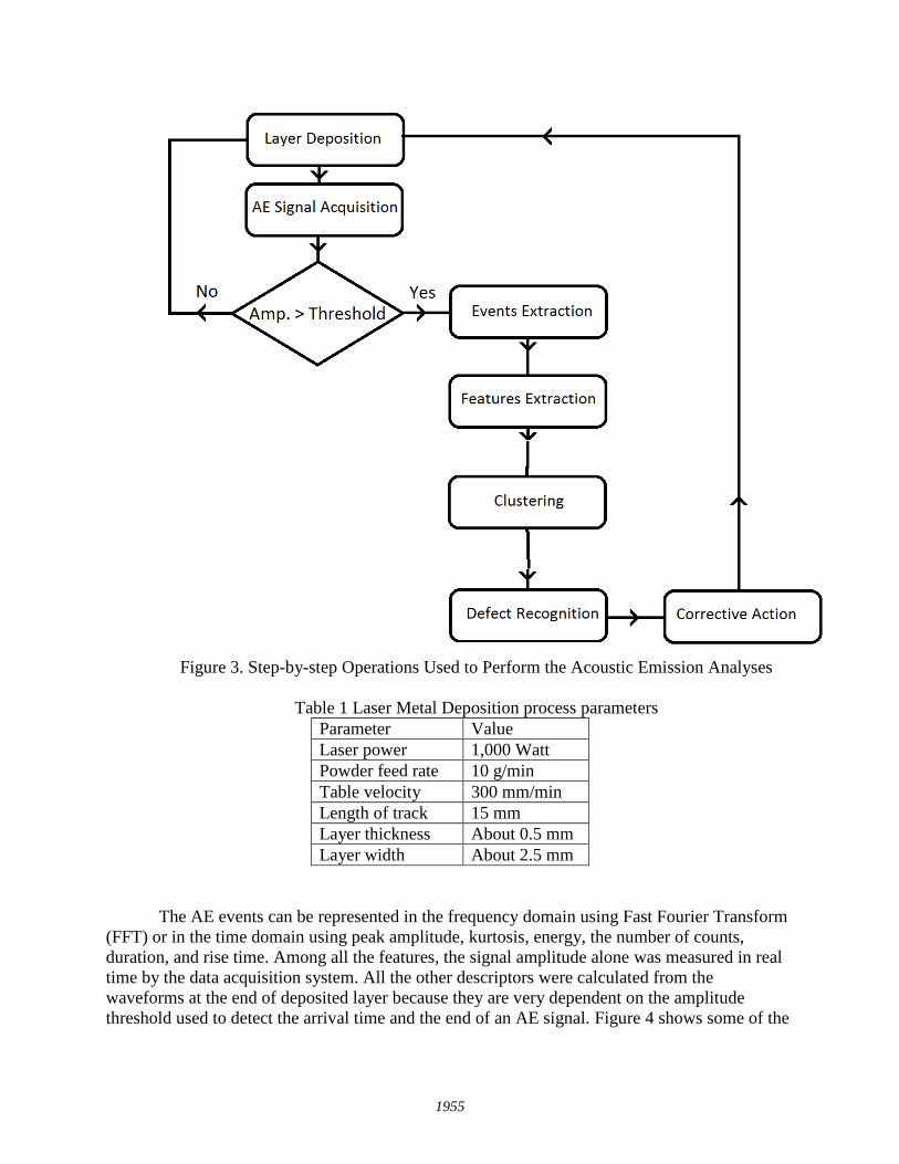
Figure 3. Step-by-step Operations Used to Perform the Acoustic Emission Analyses
Table 1 Laser Metal Deposition process parameters
Parameter Value
Laser power 1,000 Watt
Powder feed rate 10 g/min
Table velocity 300 mm/min
Length of track 15 mm
Layer thickness About 0.5 mm
Layer width About 2.5 mm
The AE events can be represented in the frequency domain using Fast Fourier Transform
(FFT) or in the time domain using peak amplitude, kurtosis, energy, the number of counts,
duration, and rise time. Among all the features, the signal amplitude alone was measured in real
time by the data acquisition system. All the other descriptors were calculated from the
waveforms at the end of deposited layer because they are very dependent on the amplitude
threshold used to detect the arrival time and the end of an AE signal. Figure 4 shows some of the
1955
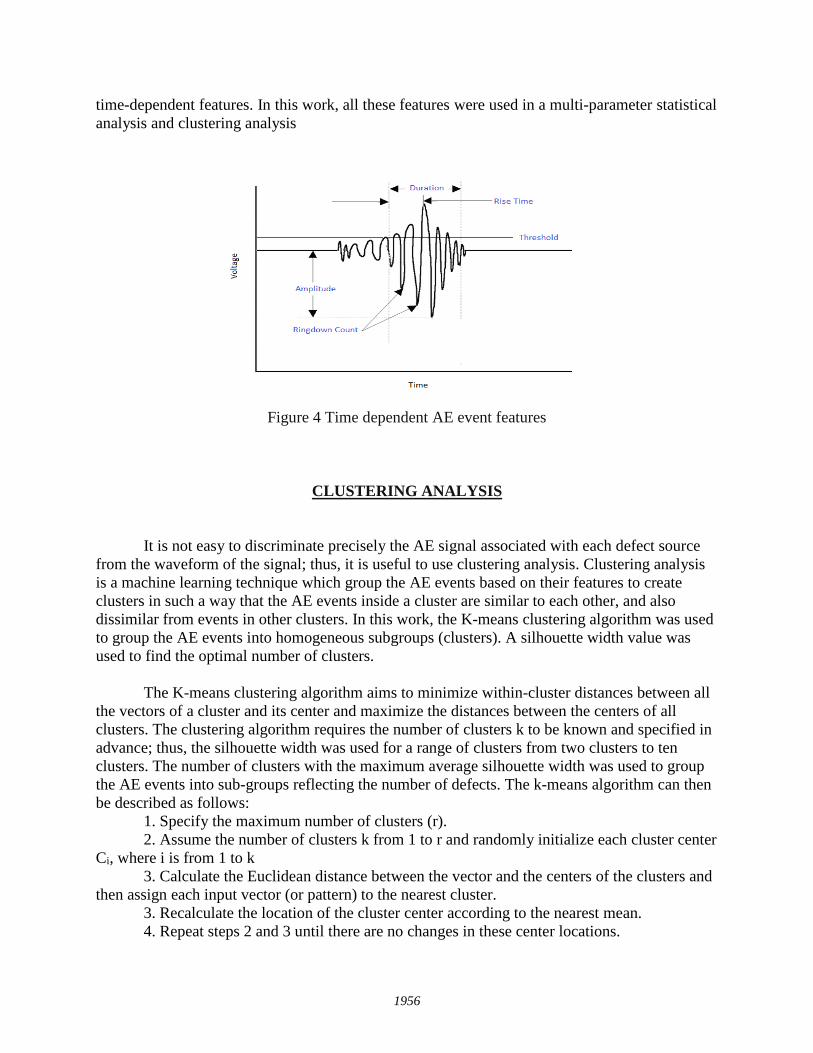
time-dependent features. In this work, all these features were used in a multi-parameter statistical
analysis and clustering analysis
Figure 4 Time dependent AE event features
CLUSTERING ANALYSIS
It is not easy to discriminate precisely the AE signal associated with each defect source
from the waveform of the signal; thus, it is useful to use clustering analysis. Clustering analysis
is a machine learning technique which group the AE events based on their features to create
clusters in such a way that the AE events inside a cluster are similar to each other, and also
dissimilar from events in other clusters. In this work, the K-means clustering algorithm was used
to group the AE events into homogeneous subgroups (clusters). A silhouette width value was
used to find the optimal number of clusters.
The K-means clustering algorithm aims to minimize within-cluster distances between all
the vectors of a cluster and its center and maximize the distances between the centers of all
clusters. The clustering algorithm requires the number of clusters k to be known and specified in
advance; thus, the silhouette width was used for a range of clusters from two clusters to ten
clusters. The number of clusters with the maximum average silhouette width was used to group
the AE events into sub-groups reflecting the number of defects. The k-means algorithm can then
be described as follows:
1. Specify the maximum number of clusters (r).
2. Assume the number of clusters k from 1 to r and randomly initialize each cluster center
Ci, where i is from 1 to k
3. Calculate the Euclidean distance between the vector and the centers of the clusters and
then assign each input vector (or pattern) to the nearest cluster.
3. Recalculate the location of the cluster center according to the nearest mean.
4. Repeat steps 2 and 3 until there are no changes in these center locations.
1956
5. calculate the maximum average silhouette width.
6. Repeat steps from 2 to 5 for all possible number of clusters.
The greater the silhouette value, the better the clustering results [7, 8]. The optimal value
of k is determined according to the maximum of the silhouette width defined as
𝑠(𝑘) =1
𝑛∑
𝑚𝑖𝑛(𝑏(𝑙,𝑘)−𝑎(𝑙))
𝑚𝑎𝑥(𝑎(𝑙),𝑚𝑖𝑛(𝑏(𝑙,𝑘)))
𝑛𝑙=1 (7)
Where 𝑎(𝑙) is the average distance between l-th event and all other events in the same cluster,
and 𝑏(𝑙, 𝑘) is the minimum of the average distances between the l-th event and all the event in
each other cluster. The silhouette width values range from -1 to 1. If the silhouette width value
for an event is about zero, it means that that the event could be assigned to another cluster. If the
silhouette width value is close to -1, it means that the event is need to be assigned to other
cluster. If the silhouette width values are close to 1, it means that the event is well clustered. A
clustering can be evaluated by the average silhouette width 𝑠(𝑘) of individual events.
The largest average silhouette width, over different K, indicates the best number of
clusters. As can be seen, in Table 2 the greatest average silhouette width is 0.8108. The number
of clusters was confirmed using Bayesian Information Criterion (BIC) [9], since it is
recommended to validate number of clusters through use of several methods. The number of
clusters with the lowest BIC is preferred which means k=2 is the optimum number of clusters.
Table 2. Average Silhouette Width for Different Number of Clusters
Number of clusters Average Silhouette Width BIC
2 0.8108 4409.199532
3 0.4730 5307.464994
4 0.4963 6268.570481
5 0.4770 7268.886407
6 0.5405 8331.531180
7 0.5004 9397.995038
8 0.4387 10464.458896
9 0.5210 11532.648846
10 0.4254 12645.626117
11 0.5346 13763.722664
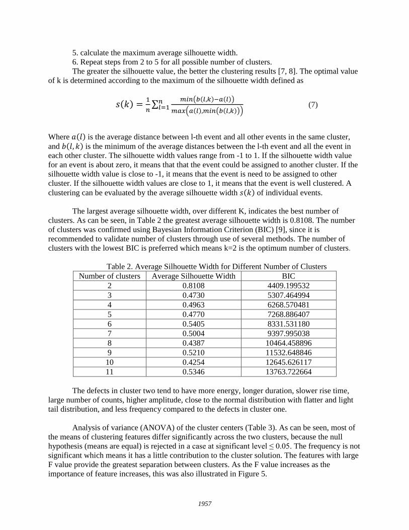
The defects in cluster two tend to have more energy, longer duration, slower rise time,
large number of counts, higher amplitude, close to the normal distribution with flatter and light
tail distribution, and less frequency compared to the defects in cluster one.
Analysis of variance (ANOVA) of the cluster centers (Table 3). As can be seen, most of
the means of clustering features differ significantly across the two clusters, because the null
hypothesis (means are equal) is rejected in a case at significant level ≤ 0.05. The frequency is not
significant which means it has a little contribution to the cluster solution. The features with large
F value provide the greatest separation between clusters. As the F value increases as the
importance of feature increases, this was also illustrated in Figure 5.
1957

Table 3. Analysis of variance (ANOVA) of the cluster centers and features importance
Cluster Error
F Sig. importance Mean Square df Mean Square df
Rise Time 30.629 1 .153 35 199.608 .000 3 Peak amplitude 29.703 1 .180 35 165.109 .000 5
Duration 30.801 1 .149 35 207.352 .000 2 Kurtosis 3.449 1 .930 35 3.709 .062 9
Number of counts 30.043 1 .170 35 176.523 .000 4 Counts to peak 28.444 1 .216 35 131.750 .000 6
Energy 31.137 1 .139 35 224.074 .000 1 Average frequency 1.184 1 .995 35 1.190 .283 10
Maximum frequency 10.870 1 .718 35 15.140 .000 8 Standard deviation of
frequencies 12.417 1 .674 35 18.429 .000 7
(a) Events in cluster one have less energy
1958
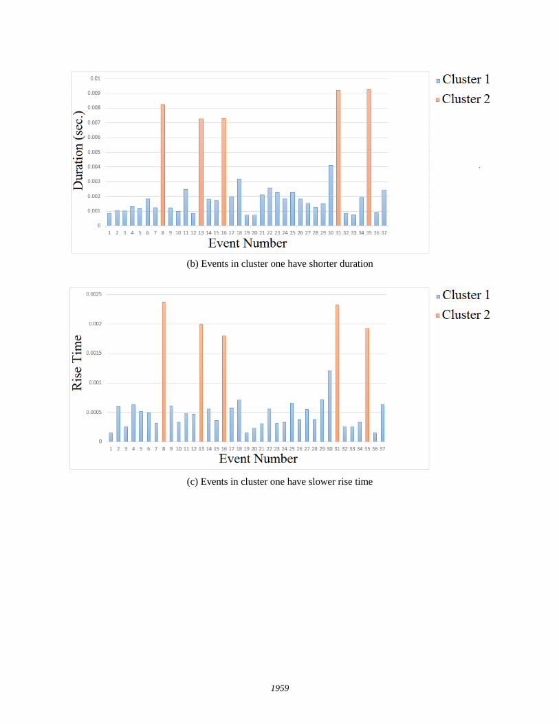
(b) Events in cluster one have shorter duration
(c) Events in cluster one have slower rise time
1959
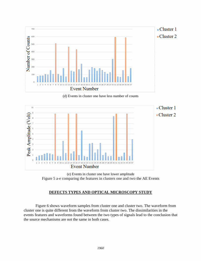
(d) Events in cluster one have less number of counts
(e) Events in cluster one have lower amplitude
Figure 5 a-e comparing the features in clusters one and two the AE Events
DEFECTS TYPES AND OPTICAL MICROSCOPY STUDY
Figure 6 shows waveform samples from cluster one and cluster two. The waveform from
cluster one is quite different from the waveform from cluster two. The dissimilarities in the
events features and waveforms found between the two types of signals lead to the conclusion that
the source mechanisms are not the same in both cases.
1960
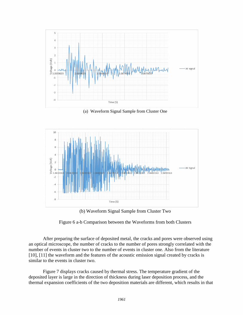
(a) Waveform Signal Sample from Cluster One
(b) Waveform Signal Sample from Cluster Two
Figure 6 a-b Comparison between the Waveforms from both Clusters
After preparing the surface of deposited metal, the cracks and pores were observed using
an optical microscope, the number of cracks to the number of pores strongly correlated with the
number of events in cluster two to the number of events in cluster one. Also from the literature
[10], [11] the waveform and the features of the acoustic emission signal created by cracks is
similar to the events in cluster two.
Figure 7 displays cracks caused by thermal stress. The temperature gradient of the
deposited layer is large in the direction of thickness during laser deposition process, and the
thermal expansion coefficients of the two deposition materials are different, which results in that
1961
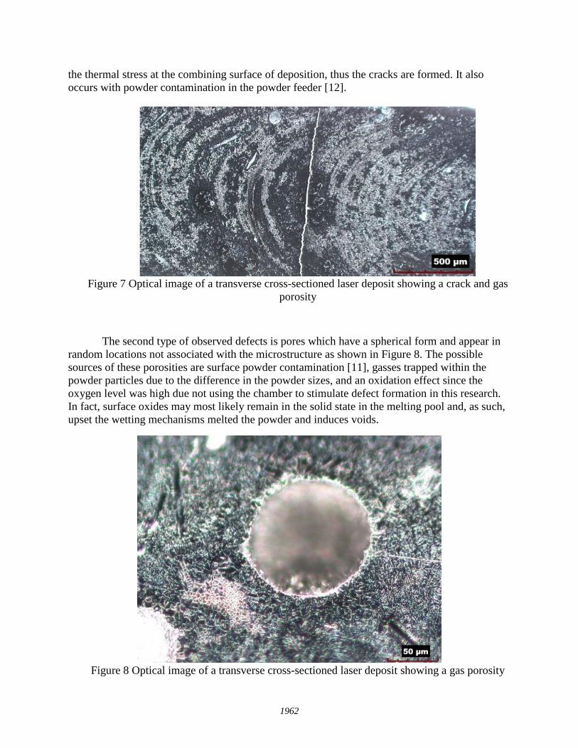
the thermal stress at the combining surface of deposition, thus the cracks are formed. It also
occurs with powder contamination in the powder feeder [12].
Figure 7 Optical image of a transverse cross-sectioned laser deposit showing a crack and gas
porosity
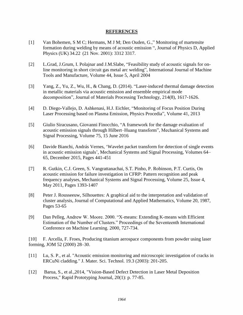
The second type of observed defects is pores which have a spherical form and appear in
random locations not associated with the microstructure as shown in Figure 8. The possible
sources of these porosities are surface powder contamination [11], gasses trapped within the
powder particles due to the difference in the powder sizes, and an oxidation effect since the
oxygen level was high due not using the chamber to stimulate defect formation in this research.
In fact, surface oxides may most likely remain in the solid state in the melting pool and, as such,
upset the wetting mechanisms melted the powder and induces voids.
Figure 8 Optical image of a transverse cross-sectioned laser deposit showing a gas porosity
1962

Conclusions
The AE signal was collected during the LMD in an oxidized environment with mixed
metal powders to stimulate all possible types of defects. Several defects mechanism were
activated and detected by AE sensor. K-Means clustering method was implemented to analyze
the AE signals and identify defects source mechanisms.
The clustering results successfully distinguish two main defects types and their signal
characteristics. The number of clusters to be created does not have to be specified in advance,
they only depend on the number of defects being created. Porosities produce the AE signals with
shorter decay time and less amplitude. The cracks trigger the AE signals with short durations and
high amplitudes. The signal energy is a crucial feature in identifying the AE defect source
mechanisms.
The validation of the proposed methodology has been carried out using an optical
microscope; it showed the correlation between the number of acoustic events and the number of
defects determined by post-test optical microscopy. The numbers of signal events are in each
cluster are in agreement with the rough estimations of the associated numbers of defects.
1963
REFERENCES
[1] Van Bohemen, S M C; Hermans, M J M; Den Ouden, G.,” Monitoring of martensite
formation during welding by means of acoustic emission “, Journal of Physics D, Applied
Physics (UK) 34.22 (21 Nov. 2001): 3312 3317.
[2] L.Grad, J.Grum, I. Polajnar and J.M.Slabe, “Feasibility study of acoustic signals for on-
line monitoring in short circuit gas metal arc welding”, International Journal of Machine
Tools and Manufacture, Volume 44, Issue 5, April 2004
[3] Yang, Z., Yu, Z., Wu, H., & Chang, D. (2014). “Laser-induced thermal damage detection
in metallic materials via acoustic emission and ensemble empirical mode
decomposition”, Journal of Materials Processing Technology, 214(8), 1617-1626.
[4] D. Diego-Vallejo, D. Ashkenasi, H.J. Eichler, “Monitoring of Focus Position During
Laser Processing based on Plasma Emission, Physics Procedia”, Volume 41, 2013
[5] Giulio Siracusano, Giovanni Finocchio, “A framework for the damage evaluation of
acoustic emission signals through Hilbert–Huang transform”, Mechanical Systems and
Signal Processing, Volume 75, 15 June 2016
[6] Davide Bianchi, András Vernes, ‘Wavelet packet transform for detection of single events
in acoustic emission signals’, Mechanical Systems and Signal Processing, Volumes 64–
65, December 2015, Pages 441-451
[7] R. Gutkin, C.J. Green, S. Vangrattanachai, S.T. Pinho, P. Robinson, P.T. Curtis, On
acoustic emission for failure investigation in CFRP: Pattern recognition and peak
frequency analyses, Mechanical Systems and Signal Processing, Volume 25, Issue 4,
May 2011, Pages 1393-1407
[8] Peter J. Rousseeuw, Silhouettes: A graphical aid to the interpretation and validation of
cluster analysis, Journal of Computational and Applied Mathematics, Volume 20, 1987,
Pages 53-65
[9] Dan Pelleg, Andrew W. Moore. 2000. “X-means: Extending K-means with Efficient
Estimation of the Number of Clusters.” Proceedings of the Seventeenth International
Conference on Machine Learning. 2000, 727-734.
[10] F. Arcella, F. Froes, Producing titanium aerospace components from powder using laser
forming, JOM 52 (2000) 28–30.
[11] Lu, S. P., et al. "Acoustic emission monitoring and microscopic investigation of cracks in
ERCuNi cladding." J. Mater. Sci. Technol. 19.3 (2003): 201-205.
[12] Barua, S., et al.,2014, "Vision-Based Defect Detection in Laser Metal Deposition
Process," Rapid Prototyping Journal, 20(1): p. 77-85.
1964


