

Demand Forecast Planner
A Manuscript
Submitted to
the Department of Computer Science
and the Faculty of the
University of Wisconsin-La Crosse
La Crosse, Wisconsin
by
Peter J. Landerud
in Partial Fulfillment of the
Requirements for the Degree of
Master of Software Engineering
December, 2009

ii
Demand Forecast Planner
By Peter J. Landerud We recommend acceptance of this manuscript in partial fulfillment of this candidate’s requirements for the degree of Master of Software Engineering in Computer Science. The candidate has completed the oral examination requirement of the capstone project for the degree. ____________________________________ _______________________ Dr. Kenny Hunt Date Examination Committee Chairperson ____________________________________ _______________________ Dr, David Riley Date Examination Committee Member ____________________________________ _______________________ Dr. Kasi Periyasamy Date Examination Committee Member

iii
ABSTRACT
LANDERUD, PETER, J., “Demand Forecast Planner”, Master of Software Engineering,
December 2009, (Dr. Kenny Hunt).
Hy Cite Corporation, a small company by many standards, has over 1,900 currently
active and sellable products. Those active products account for 1.19 million physical
items totaling $37.9 million dollars in total inventory. Roughly $40 million dollars in
working capital is a lot of money to have tied up, and upper management has been
putting a lot of pressure on the purchasing department to reduce inventory costs. The
threat of running out of inventory to fulfill orders is the greatest risk of trying to reduce
inventory. More accurate reporting of sales and inventory is needed to reduce this risk. A
tool is needed to judge the demand for these products and forecast future inventory
purchases. This document describes the software lifecycle used to create such a tool,
Demand Forecast Planner, which assists the purchasing department in planning inventory
needs.

iv
ACKNOWLEDGEMENTS
I would like to first thank my fiancée, Marki, for all of her support. As I have struggled
with this project and the MSE program she has always been there to support me. Having
struggled with reading and writing all my life, I would also like to thank her for the
countless hours she spent proof reading this thesis, correcting numerous spelling and
grammatical errors.
Secondly, I would like to thank my parents Dave and Jacqui. Growing up with the love
and support of two great parents has made more of a difference in life than I ever could
have imagined. Instilling a good set of moral values, a can do attitude and a good work
ethic has done more to make me successful in life than anything else. Additionally
growing up with a learning disability it would have been easy for me to forgo advanced
academics, but my parents, as well as exceptional teachers, ensured I never felt like there
was anything I could not do.
Finally I would of course like to the Computer Science Department, and specifically Dr.
Kenny Hunt and Dr. David Riley for all their help with my thesis and being overall
excellent professors who I have learned a great deal from. The Computer Science
Department at the University of Wisconsin La Crosse has a truly great program that has
more than adequately prepared me for a career in the field of software engineering.

v
TABLE OF CONTENTS
Page
ABSTRACT……………………………………………………………………………. iii
ACKNOWLEDGEMENTS………………………………………………………....…..iv
TABLE OF CONTENTS…………………………………………………………...…....v
LIST OF TABLES…………………………………………………………………...... vii
LIST OF FIGURES…………………………………………………………………... viii
1. Introduction …………………………………………………………………………. 1
1.1 Commercial Software Downfalls ……………………………………...………. 2
1.2 Project Goals ……………………………...…………………………………….3
1.3 Project Personnel .....……………………………………………………………..3
2. Software Life Cycle Models ………………………………………………………... 4
3. Requirements ………………………………………………………………………... 6
3.1 Requirements Gathering Methodology .………………………………….…..... 6
3.2. Requirements Gathering – Demand Forecast Planner ……………………...…. 9
3.3 Functional Requirements Overview …………………………………………. 11
3.3.1 Terms Supporting Functional Requirements …………………...……..... 11
3.3.2 Functional Requirements for Warehouse ……………………………..... 16
3.3.3 Functional Requirements for Product ………………………………...… 17
3.3.4 Functional Requirements for Warehouse Product ……………………… 18
3.3.5 Functional Requirements for Profile ……………………………………. 19
3.4 Lessons Learned During Requirements Gathering.……………………………. 20
4. Design .…………………………………………………………………………........ 22
4.1 Design Methodology ………....……………………………………………….. 22
4.2 Designing the Demand Forecast Planner …………………………………...…. 25
4.2.1 Class Design Overview ………………………………………………….. 26
vi
4.2.2 Database Design Overview ……………………………………………... 30
4.3 Lessons Learned During Design ……………...………………………………. 32
5. Coding ………….…………………………………………………………………... 35
5.1 Methodology/Coding the Demand Forecast Planner …………………………. 35
5.2 Code Metrics for the Demand Forecast Planner …………………………….... 39
6. Testing ……. ………………………………………………………………………. .41
6.1 Testing Methodology …………………………………………………………. 41
6.2 Testing the Demand Forecast Planner ………………………………………... 42
6.3 Lessons Learned During Testing ……………………………………………... 50
7. Maintenance ……………………………………………………………………….. 52
7.1 Maintenance Methodology …………………………………………………… 52
7.2 Maintaining the Demand Forecast Planner ………………………………….... 53
7.3 Lessons Learned During Maintenance ………………………………………... 58
8. The Demand Forecast Planner Application ………………………………………… 60
9. Continuing Work ...…………….………………………………………………….... 66
10. Conclusion …………………………………………………………………………. 67
11. Bibliography ……………………………………………………………………….. 69

vii
LIST OF TABLES
Table Page
3.3 Global Purchasing Terms ………………………………...……………………..13
3.4 Period Based Purchasing Terms for Sales ……...…………………………........14
3.5 Period Based Purchasing Terms for Inventory ……………………………....... 16
3.6 Functional Requirements for a Warehouse ……………………………………..17
3.7 Functional Requirements for a Product ……………………………………….. 18
3.8 Functional Requirements for a Warehouse Product …………………………... 19
3.9 Functional Requirements for a Profile ………………………………………… 20
5.1 Variable Guidelines and Best Practices ……………………………………….. 36
5.2 Readability, Complexity and Understandability Guidelines ………………….. 37
5.6 Error Handling and Library Usage Guidelines ………………………………... 39
6.1 Fictional Product Test Data …………………………………………………… 43
6.2 Test Cases for Fictional Product TST01 ………………………………………. 45
6.3 Product Data for CO6323 (9 Ply, 10 Piece Cookware Set) …………………… 47
6.4 Test Cases for CO6323 (9 Ply, 10 Piece Cookware Set) ……………………… 49
7.2 Updated Terms for Change Request …………………………………………... 55

LIST OF FIGURES
Figure Page
3.1 Requirements Gathering Model ………....……………………………………. 7
3.2 Excel Based Prototype …………..………………………………………….... 11
4.1 Design Model ……………………………………………………………….... 23
4.2 Class Diagram ...……………………………………………………………... .27
4.3 Entity Relationship Diagram 1 .…………………….……………………….... 30
4.4 Entity Relationship Diagram 2 .…………………….……………………….... 31
5.3 Standard Comment Block ……………………………………………………. 38
5.4 Regions and Logically Grouping Code Elements ……………………………. 38
7.1 First Enhancement Request ……………………………………………………54
7.3 Updated Requirements for Change Request ………………………………...... 55
7.4 Updated Class Design for Change Request …………………………………... 56
7.5 Updated Source Code for Change Request ………………………………….... 57
7.6 Source Code Control Comparison ……………………………………………. 57
8.1 Product Selection Form ……………………………………………………….. 60
8.2 Demand Forecast Planner Form (Summary and Sales Information) ………….. 61
8.3 Demand Forecast Planner Form (Inventory Information) …………………….. 62
8.4 Color Setup Form ……………………………………………………………... 64
8.5 Plan Transfer In Units By Warehouse Report ………………………………… 65

GLOSSARY
Article (Article ID)
The alphanumeric value used internally to identify a product. Also called Product Code.
Avg Cost (Average Value)
The average cost of all products in inventory. For any one item, the landed cost can
fluctuate based on shipping method, country of origin, 1st cost changes, etc.
Avg Inventory (Average Inventory)
Average Inventory that is in stock for a specific period of time.
Avg Sls Units (Average Sales Units)
The average predicted units to be sold per period based on the future year of predicted
sales.
BOH Qty (Beginning On Hand Quantity)
Beginning On Hand Quantity - units available at the beginning of the current period.
Cost (Purchase Price)
1st cost of an item. This is the actual cost that we pay for the product, it does not include
domestic or international freight, duties, customs fees, etc.
Lead (Lead Time)
Required timeframe between purchase order (PO) placement and PO delivery. This
includes production and shipping timeframes.
Product Group
The group that a given product belongs to. For example CO6301 (9 Ply 5 piece
Cookware set) belongs to the Cookware product group.
PPY Sls (Prior Prior Year Sales)
The number of units sold in the prior prior year for a given period or sales from two years
ago.
PY BOP (Prior Year Beginning of Period)
The number of units that were on hand at the beginning of the period in the prior year.
PY EOP (Prior Year End of Period)
The number of units that were on hand at the end of the period in the prior year.
PY Plan Sls (Prior Year Planned Sales)
The planned number of units that were predicted to be sold for one year prior to a given
period.
PY Plan Sls As % PY Sls (Prior Year Planned Sales as percent of Prior Year Sales)
Prior year plan sales expressed as a percent of prior year sales.
PY Received (Prior Year Received)
The number of units received the prior year for a given period.
PY RTS (Prior Year Return To Stock)
The number of units returned to stock the prior year for a given period.
PY Sls (Prior Year Sales)
The number of units sold the prior year for a given period.
PY Sls As % PPY Sls (Prior Year Sales as a percent of Prior Prior Year Sales)

Prior year’s sales expressed as a percent of prior prior year sales.
PY Sls As % PY Plan Sls (Prior Year Sales as percent of Prior Year Planned Sales)
Prior year’s sales expressed as a percent of prior year’s planned sales.
PY Tot Sales (Prior Year Total Sales)
Total units that were sold over the past one year.
PY Turn (Prior Year Turn)
Prior year turn for the current period.
Total Units On Order
Total units for a particular item that are on existing, approved purchase orders.
Turn
Number of times inventory is replenished; generally calculated by dividing the average
inventory level (or current inventory level) into the inventory usage.
TY Act/Plan BOP (This Year Actual/Planned Beginning of Period Units on Hand)
This year actual units that are on hand at the beginning of the current period or the
planned beginning of period units for any future period.
TY Plan EOP (This Year Plan End Of Period)
This year’s planned end of period units on hand.
TY Plan Sls (This Year Planned Sales)
Total units planned to sell this year.
TY Plan Sls As % PY Sls (This Year Planned Sales as a percent of Prior Year Sales)
This year’s planned sales expressed as a percent of prior year’s sales.
TY Plan Turn (This Year Planned Turn)
The planned turn for this year for a given period.
TY Project Sales (This Year Projected Sales)
Total units that are projected to be sold over the next one year.
Vendor
The name of the company or merchant we purchase a given product or set of products
from.
Vendor Item (Vendor Product ID)
The alphanumeric value our vendor uses to identify a product.
1
1. Introduction The direct sales industry, much like the retail industry, depends on a large
inventory to be successful. Avon and Tupperware are two commonly known
players in the direct sales industry. These two companies, like the company
requesting this project, illustrate the importance inventory plays in this type of
business. Tupperware, for example, does not manufacture much of its inventory in
the same country in which it is sold. A great deal of manufacturing is done in
places like China, where turn-around time between when the product is ordered to
when it is actually received can be months.
The distributor network that is in charge of selling products for a company like
Tupperware has very little insight, if any, into the inventory levels of products
they are selling. The distributors are independent of the company itself and by
design only need to concern themselves with making sales. Everything else is the
responsibility of the company employing the distributor. This makes work easier
for the distributor, but puts a great deal more responsibility on the company
supporting them to have inventory available when it is needed.
In order to support sales, a large supply of inventory is needed to prevent units
from going on back-order and customers having to wait for months before getting
their products. The best way to predict future inventory requirements is to look at
past sales and inventory levels along with consumer trends. When these figures
are thought to be less reliable, greater inventory is typically kept on hand to
ensure there is enough to meet sales demand.
The amount of money tied up in inventory is something every company wants
to minimize, and because of this, the issues stated above cannot be simply solved
by ordering an excess supply of inventory. While there is no easy way to
minimize working inventory costs and still maintain sufficient inventory to meet
demand, one universal truth is that precise, current, and easily accessible data on
past sales, inventory and consumer trends is essential to accurately predict future
inventory needs.

2
1.1 Commercial Software Downfalls Critical to the success of the company requesting this project are two major
commercial software packages. The first is Agresso, and it is used to track
accounting related data. This software system tracks sales orders when a product
is sold and purchase orders for products purchased from vendors. Agresso also
tracks how much inventory is on hand, as well as managing a number of other
data sets related to both sales and inventory.
The second software system is Highjump; it is used to track the location and
quantity of inventory within the warehouse. Highjump is supplied sales orders
from the Agresso system and it manages the physical storage locations for all
items in inventory. This information is used to direct warehouse employees to the
locations of specific items when filling orders. Highjump tracks data from two
warehouses – one in Madison, WI, and one in Guadalajara, Mexico.
Both of these software systems are excellent at what they were designed to do
and they collect considerable raw data regarding past sales and consumer trends.
However, the data within these systems is scattered across fifteen to twenty
different locations. Furthermore, these systems lack any type of historical
inventory data. They adequately identify current stock, but do not maintain
information regarding past stocking levels.
The Purchasing Department tracks the data needed to make purchasing related
decisions. Data aggregated from the above systems is compiled into a set of Excel
spreadsheets which are used for inventory management. This process is extremely
time consuming and often yields inaccurate information for predicting future sales
and inventory needs.

3
1.2 Project Goals
The goals of this project are to create a GUI tool, named Demand Forecast
Planner, which can be used by the Purchasing Department to place orders for
future inventory needs. This tool should aggregate data from several systems into
one centralized application previously scattered across multiple locations. This
data can then be analyzed and manipulated to predict inventory needs. The above
goals, along with the amount of manual time that was being spent to complete this
process, were the reasons for moving forward with this project.
Additional goals internal to the IT Department were to create understandable
classes that would abstract the raw data being used by the Purchasing Department
from the database. Too often, applications are built directly on top of databases
without first abstracting the data into something more easily understood. This
causes issues in both understandability as well as maintainability. Knowing this
project will be expanded over the years, it was critical to design the project with
expansion in mind.
1.3 Project Personnel Two teams were involved in the creation of the Demand Forecast Planner - the
Development Team which consisted of software engineer, Peter Landerud, and
the customer which consisted of the purchasing manager, Kara Moorhouse. Both
groups are employed by Hy Cite Corporation, and work out of the Madison, WI
office. Peter Landerud has been a software engineer for five years with a
background in thick client and web application development using Microsoft .Net
technologies. Kara Moorhouse has over fifteen years of purchasing experience,
and has worked for retail companies such as ShopKo as well as direct sales for Hy
Cite.

4
2. Software Life Cycle Models
A number of different software life cycle models exist, each with its own set of
advantages and disadvantages. The one chosen for this project was the iterative
prototype model. The main reason for using a prototyping model was because of
the effective feedback that can be generated by having an actual program in front
of the customer. This, in conjunction with the fact that the customer of this project
worked in the same building as the Development Team, made prototypes easy to
release and made it convenient to receive feedback from the customer.
An additional reason for using a prototyping model was the lack of leverage the
Development Team has on its customers to provide adequate requirements. The
job of IT is to support the business functions of departments within a company.
This is a vastly different role than that of a commercial software company. If a
traditional waterfall model would have been used, more responsibility would have
been placed on the customer to come up with complete requirements. As the
Development Team for this project had little recourse to ensure the customer
provided complete requirements, a prototyping model was used to collect more
complete requirements.
Internal departments are generally willing to provide requirements to a
moderate degree of detail, but usually it is the Development Team’s job to clarify
those requirements into what the customer actually wants. In the past experience
of the Development Team, it was found that the easiest and most effective way to
accomplish this was to get what requirements one could from the customer
without pushing too hard and then develop a prototype to clarify the requirements.
The feedback received from the prototype paired with the upfront requirements
generally would deliver a successful application that would meet the customer’s
needs.
With all software life cycle models there are trade-offs, and the iterative
prototype model is no exception. While direct customer feedback from a
prototype is extremely useful to the Development Team, it can also lead to a great

5
deal of throw-away work. Gathering clear, unambiguous requirements is a
difficult task to master, and one that the Development Team for this project is still
working to improve. Trying to build a prototype around less than complete
requirements can lead to incorrect or unwanted functionality. Additionally, the
time spent implementing this functionality into a prototype is ultimately thrown
away and may have been avoidable with more complete upfront requirements.
Even with the potential for a fair amount of throw-away work, an iterative
prototyping model was determined to be the best choice for this project. It
provided a way of clarifying initial requirements defined by the customer and also
helped the Development Team to identify better ways to clarify requirements up
front.

6
3. Requirements
The first, and many times most, important phase of software development is
requirements gathering. IEEE has the following definition for a requirement: [6]
“
1. A condition or capability needed by a user to solve a problem or
achieve an objective.
2. A condition or capability that must be met or possessed by a system or
system component to satisfy a contract, standard, specification, or other
formally imposed documents.
3. A documented representation of a condition or capability as in (1) or
(2).
”
This definition suggests that a set of requirements is a document, or set of
documents, that define(s) the behavior of a software system. Gathering correct
requirements is critical because it defines what the software being built is required
to do and is the foundation on which all other software life cycle phases will be
built upon. IEEE states “poorly defined system requirements” as one of the
leading causes of why software systems fail [10].
3.1 Requirements Gathering Methodology For the reasons given in section 2, the model shown in figure 3.1 was used to
define the requirements for the Demand Forecast Planner.
7
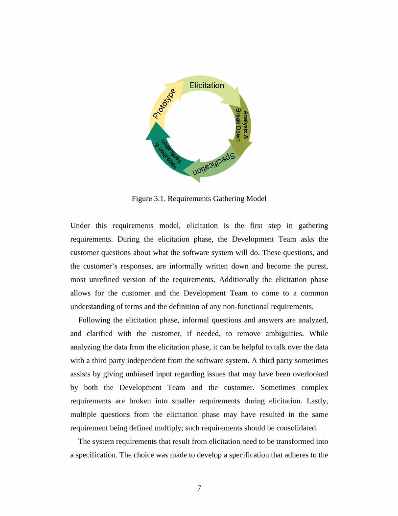
Figure 3.1. Requirements Gathering Model
Under this requirements model, elicitation is the first step in gathering
requirements. During the elicitation phase, the Development Team asks the
customer questions about what the software system will do. These questions, and
the customer’s responses, are informally written down and become the purest,
most unrefined version of the requirements. Additionally the elicitation phase
allows for the customer and the Development Team to come to a common
understanding of terms and the definition of any non-functional requirements.
Following the elicitation phase, informal questions and answers are analyzed,
and clarified with the customer, if needed, to remove ambiguities. While
analyzing the data from the elicitation phase, it can be helpful to talk over the data
with a third party independent from the software system. A third party sometimes
assists by giving unbiased input regarding issues that may have been overlooked
by both the Development Team and the customer. Sometimes complex
requirements are broken into smaller requirements during elicitation. Lastly,
multiple questions from the elicitation phase may have resulted in the same
requirement being defined multiply; such requirements should be consolidated.
The system requirements that result from elicitation need to be transformed into
a specification. The choice was made to develop a specification that adheres to the

8
IEEE 830-1998 standard [7]. During this phase, the analyzed data is formed into
functional system requirements and non-functional system requirements.
The formal requirements defined in the specification phase need to be validated
against the original elicitation information, with the customer and possibly with
an additional third party. The first step after formal requirements have been
specified is to validate that requirements meet the data defined in the elicitation
phase. The requirements must ensure the elicitation information is fully captured,
and must also ensure additional requirements are not added, because development
team prejudice might result in items that the customer did not specifically define.
Additionally, during this phase the Development Team needs to verify the defined
requirements with the customer. Often elicitation information is lost in translation
and should be verified before any prototyping or design work begins. It can also
be beneficial to verify the requirements with a third party. A third party should be
able to understand the requirements defined, and if not, additional work is needed
to clarify the requirements.
The last step in this requirements model is to create a prototype that
implements most or all of the functional requirements defined. The goal of this
prototype is to help further refine the requirements of the software system. For
this reason, it is not essential to implement all the requirements into the prototype.
Additionally, this prototype is throw-away code and the amount of design put into
how it is created should be greatly limited; this is only a tool to help gather more
complete requirements.
Once the prototype is complete, the process starts again with the elicitation
phase, but the questions asked during this phase should be driven by the prototype
developed in the previous iteration. The customer, while using the prototype, can
explain how the final software system should be similar to or different from the
prototype. This elicitation information will be used to again start the requirements
gathering phase. The process of creating iterations of prototypes is one with
9
greatly diminishing returns and the number of prototypes created before moving
onto the design phase should be limited as these prototypes are throw-away work.
3.2 Requirement Gathering - Demand Forecast Planner
During the elicitation phase for the Demand Forecast Planner, the customer and
the Development Team had several face-to-face meetings where the requirements
of the software system were discussed. Purchasing, much like software
engineering, has its own set of terms and acronyms. The initial few meetings were
spent getting the Development Team up to speed on the ins-and-outs of
purchasing. Software engineers and developers are often asked to create
applications within domains that are unfamiliar to them. In order for adequate
requirements to be defined, both the customer and the Development Team must
have some common level of understanding about the application domain. In the
case of this application the establishment of that common ground took several
meetings for the Development Team to understand.
After common terms and the initial requirements were discussed, this
information was analyzed and a formal requirements document was created that
adhered to the IEEE 830-1998 standard [7]. A separate document was created to
hold the non-functional requirements. These documents were reviewed by the
Development Team as well as a third party member of the IT department before
they were delivered to the customer for verification. During the verification
process with the customer, a few requirements changed and several new
requirements were added. The resulting requirements document was reviewed,
and it was determined an adequate prototype could be created using Excel. While
the final system would not be implemented in Excel, it was determined that a
simple Excel prototype could be created that would save a great deal of time. As
this prototype would be thrown away after the requirements phase, it made sense
to develop something quickly even if it would be different from the final system.
10
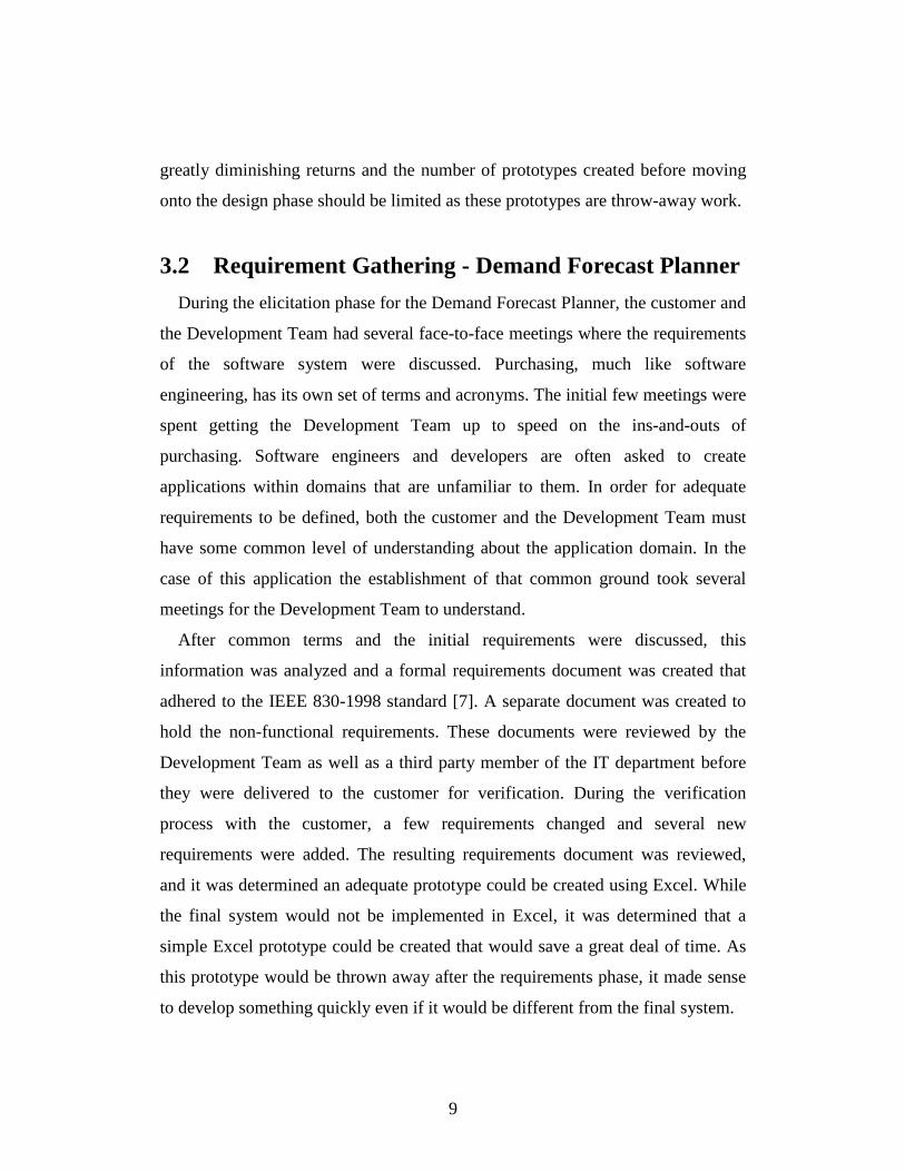
This prototype was then reviewed by the customer and the above process was
repeated. The prototype was updated with new and changed requirements. After
the second iteration of the prototype, it was determined the requirements were
sufficient to move on to the design phase. The resulting requirements document
consisted of 51 terms and 16 functional requirements. No formal GUI
requirements where defined, but the Excel prototype (Figure 3.2) was used to
define initial GUI requirements. The prototype could have been translated into
formal GUI requirements, but the benefit of such an action was seen as wasteful,
as GUI requirements were a small part of this application and functionality was its
major concern.

11
Figure 3.2 Excel Based Prototype
(The images shown above would span one row, but are broken apart for visibility)
3.3 Functional Requirements Overview
This section will give a high level overview of the functional requirements and
terms defined in the initial requirements phase of the Demand Forecast Planner.
The information shown here is in no way the complete set of requirements
defined for the Demand Forecast Planner, and for such information the formal
software requirement specification [2] should be referenced.
3.3.1 Terms Supporting Functional Requirements
These were the terms defined within the first several days of requirements
gathering. These terms helped establish a common understanding of the
application domain that could be built upon to establish functional requirements.
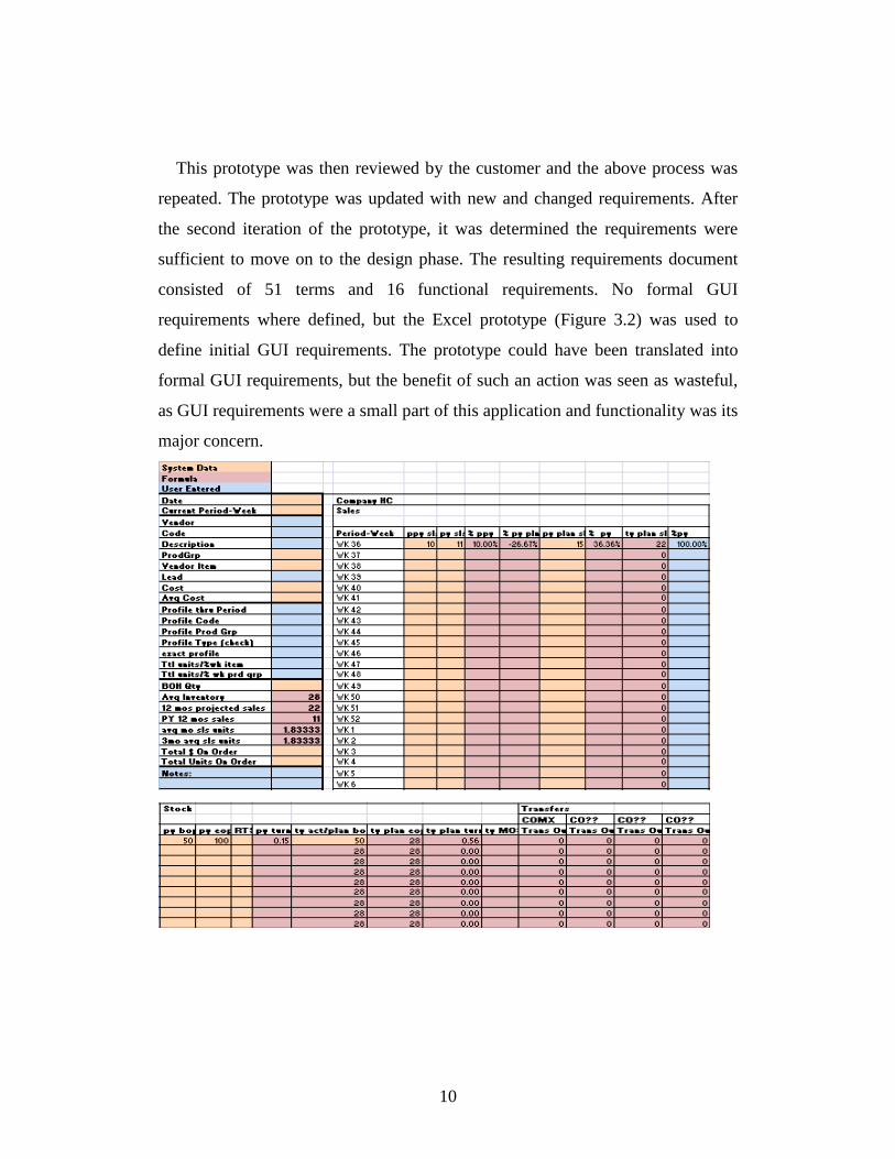
Global Purchasing Terms Term Definition Calculation/Reference Current Period-Week
The current week number and the date the current week started on (i.e. 200838 – 9/17/08)
None
Vendor The vendor we purchase a given product from.
Agresso.ASUHEADER.APAR_NAME
Product Code (Article/Article ID)
The article and article ID we use to identify a product.
Agresso.ALGARTICLE.ARTICLE
12
Product Description The description of the product. Agresso.ALGARTICLE.ART_DESCR
Product Group The product group of the product.
Agresso.ALGARTICLEGR.DESCRIPTION
Vendor Item (vendor product ID)
The code the vendor uses internally to identify the item. This will default to our internal article until purchasing manually updates this value within Agresso.
Agresso. APOPRICE.ARTICLE
Lead (Lead Time) Required timeframe between PO placement and PO delivery - includes production and shipping timeframes.
None
Cost (Purchase Price)
1st cost of an item - this is the actual cost that we pay for the product, it does not include domestic or international freight, duties, customs fees, etc.
Agresso. ASTARTVALUE.UNIT_PRICE
Avg Cost (Average Value)
The average cost of all products in inventory. For any one item, the landed cost can fluctuate based on shipping method, country of origin, 1st cost changes, etc.
ALGARTICLE.UNIT_VALUE
Profile Type The type of profile that will be used to predict future sales.
None
Profile thru Period If a profile is used this date would indicate when the profile would cease and the items own history would start. I.E. use the profile product to gets PY Sls until this date is reached.
None
Profile Code An active code (article/article ID) with 12mos+ selling history that could be used to model history for a new code.

13
BOH Qty (Beginning On Hand Quantity)
Beginning On Hand Quantity - units available at the beginning of the current period. This information should be pulled out of Agresso.
Sum all FIFO layers within WeeklyStockLevels for the current period/article.
Avg Inventory Average Inventory that is in stock for a specific period of time - for this application it would be the future 52 weeks.
BOH Qty for the future 52 weeks / 52.
52 Week Projected Sales (TY Projected Sales)
Total units that are projected to be sold as of the current date for the next 52 weeks.
Sum of this year’s planned sales (TY PLAN SLS) for the next 52 weeks.
PY 52 Week Sales Total units that were sold for the previous 52 weeks.
Sum of last year’s sales (PY SLS) 52 weeks.
Avg Weekly Sls Units (Average Units Sold Per Period)
Average weekly sales units based on the 52 weeks future.
Sum of this year’s planned sales (TY PLAN SLS) for the next 52 weeks divided by 52.
12 Week Avg Sls Units (Average Units Sold Over Next 90 Days)
Average Weekly sales units based on the 12 week future.
Sum of this year’s planned sales (TY PLAN SLS) for the next 12 weeks divided by 12.
Total Units On Order
Total units for a particular item that are on existing, approved purchase orders.
PO’s where the Rev Delivery Date is in the future
Notes Area where the user can make notes that pertain to the product, demand planning process that can be saved and will appear when the code is brought up again.
None
Table 3.3 Global Purchasing Terms
The following terms define shorthand used by the Purchasing Department to
represent sales data during a given period of time. All terms are defined based on
a week timeframe in the past, present or future. For example, PY Sls (prior year

14
sales) defines how many of a given item was sold during a week timeframe last
year.
Period Based Purchasing Terms For Sales Term Definition Calculation/Reference PPY Sls Prior prior year sales for a
specific period. None
PY Sls Prior year sales for a specific period.
None
PY Sls As % PPY Sls
Prior year’s sales expressed as a % +/- prior prior years sales.
(PY Sales/PPY Sales) – 1
PY Sls As % PY Plan Sls
Prior year’s sales expressed as a % +/- prior years planned sales.
(PY Sales/PY Plan Sls) – 1
PY Plan Sls Prior year planned sales. None
PY Plan Sls As % PY Sls
Prior year plan sales expressed as a % +/- prior year sales.
(PY Plan Sls/PY Sales) - 1
TY Plan Sls Total units planned to sell this year.
(PY Sls) * ((TY Plan Sls As % PY Sls) + 1)
TY Plan Sls As % PY Sls (% PY)
This year’s plan sales expressed as a % +/- prior year’s sales.
PY Sales/PPY Sales – 1
Table 3.4 Period Based Purchasing Terms for Sales
The following terms define shorthand used by the Purchasing Department to
represent inventory data during a given period of time. All terms are defined
based on a week timeframe in the past, present or future. For example, PY BOP
(prior year beginning of period on hand units) defines how many of a given item
was on hand during the beginning of the weekly period last year.
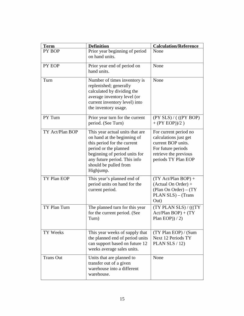
Period Based Purchasing Terms For Inventory
15
Term Definition Calculation/Reference PY BOP Prior year beginning of period
on hand units. None
PY EOP Prior year end of period on hand units.
None
Turn Number of times inventory is replenished; generally calculated by dividing the average inventory level (or current inventory level) into the inventory usage.
None
PY Turn Prior year turn for the current period. (See Turn)
(PY SLS) / ( ((PY BOP) + (PY EOP))/2 )
TY Act/Plan BOP This year actual units that are on hand at the beginning of this period for the current period or the planned beginning of period units for any future period. This info should be pulled from Highjump.
For current period no calculations just get current BOP units. For future periods retrieve the previous periods TY Plan EOP
TY Plan EOP This year’s planned end of period units on hand for the current period.
(TY Act/Plan BOP) + (Actual On Order) + (Plan On Order) – (TY PLAN SLS) – (Trans Out)
TY Plan Turn The planned turn for this year for the current period. (See Turn)
(TY PLAN SLS) / (((TY Act/Plan BOP) + (TY Plan EOP)) / 2)
TY Weeks This year weeks of supply that the planned end of period units can support based on future 12 weeks average sales units.
(TY Plan EOP) / (Sum Next 12 Periods TY PLAN SLS / 12)
Trans Out Units that are planned to transfer out of a given warehouse into a different warehouse.
None

16
Trans In Units that are planned to transfer into this warehouse from a different warehouse.
None
PY Received Prior year units received during the current period last year.
None
Actual On Order Actual units currently on an approved purchase order for that period.
None
Plan On Order Additional units needed - or order planned to be placed for that period.
None
Table 3.5 Period Based Purchasing Terms for Inventory
The terms from Table 3.5 define the data metrics of interest to the Purchasing
Department for properly predicting future inventory needs. Several of these terms
were defined directly from an existing system, and some were calculated based on
data from existing systems. Other terms are independent of prior systems and
defined only with reference to the Demand Forecast Planner. A number of
calculations were known by the Purchasing Department, and listed where
available, but some terms needed to be calculated by the Demand Forecast
Planner and those calculations were defined in the design phase.
The intent of defining the terms was to establish what the customer wanted, not
how to actually implement these items. This line became somewhat blurred
during this process; for example, what the customer wanted was a data metric
called "Prior Year Turn". The calculation of the value could be viewed as design
detail that should be defined within the design phase, but Prior Year Turn is better
understood when the context is provided. During this process the development
team worked hard to keep what the customer wanted separate from how it would
actually be implemented, but like the example given above some overlapping
occurred.
3.3.2 Functional Requirements for Warehouse

17
During the process of defining the requirements, the concept of being able to
represent a warehouse arose. Previously, the Excel documents used to predict
sales had no concept of a warehouse. Units sold for a given item were simply
aggregated, even though some of the units were from different warehouses. This
was acceptable since the sales from the Mexico warehouse were relatively small.
As the Mexico warehouse increased in sales growth, this lack of warehouse
distinction became more of an issue and was on the top of the list for
requirements.
Requirement Name Requirement Description
Create Warehouse Create a virtual location, referred to as a warehouse,
which represents a physical location where stock is shipped to and/or sold from. When showing/predicting sales and inventory for a product a warehouse will further break down the sales and inventory for that product by a location. This location, referred to as warehouse, represents the current operations in the US and Mexico.
Modify Warehouse Modify an existing warehouse.
Remove Warehouse Remove an existing warehouse.
Table 3.6 Functional Requirements for a Warehouse
3.3.3 Functional Requirements for Product A product is a physical item that is sold by or used for replacement parts at the
company. The data elements that represent these items are already tracked within
systems in the company, but the concept of being able to use the Demand
Forecast Planner to predict future sales and inventory is one that does not apply to
every product. For this reason a product in the context of the Demand Forecast
Planner is an existing product the Demand Forecast Planner is allowed to predict
sales and inventory needs for.

18
Requirement Name Requirement Description
Create Product Creates a new product that can be used by the demand
forecast planner. Remove Product Remove an existing product.
Table 3.7 Functional Requirements for a Product
3.3.4 Functional Requirements for Warehouse Product A warehouse product is a specific physical item sold or stored at a specific
physical location over a given amount of time. For example, how many of product
code 1234 were sold out of the Madison warehouse during the sixth week of 2008
would be the kind of data a Warehouse Product would contain. The idea of
breaking out sales and inventory for a specific item by location was a function the
previous system did not have. The primary focus of the Demand Forecast Planner
is to view sales and inventory data based on a weekly period, but the ability to
view this information on a monthly period is also needed. For this reason a
warehouse product also represents a specific amount of time or time period, be it
weekly or monthly.
Requirement Name Requirement Description
Create Warehouse Product
To create the relationship between warehouse and product. A warehouse product represents a specific product being stored, shipped and sold from a given warehouse. It further breaks down those sales based on Period Type. The main focus of this application is to see sales and inventory on a weekly basis, but the option to view them on a monthly basis is also needed.
Retrieve Warehouse Product Details
Based on the product and warehouse retrieve product info.
Get Past Sales To get the past 2 years (104 weeks, or 24 months) of sales for this warehouse product. The past 2 years of sale are retrieved from the database for this warehouse product. If there are not 2 years of sales present retrieve whatever history is available.

19
If there is a profile in place for this product, get past sales based on the profile details.
Calculate Past Sales Metrics
To calculate a set of metrics based on past sales.
Get Past Inventory Levels
To get the past 1 year (52 weeks or 12 months) of inventory levels for this warehouse product. The past 1 year of inventory for this warehouse product is retrieved from the database. If there is not 1 year of inventory present, retrieve whatever history is available. If there is a profile in place for this product, get past inventory based on the profile details.
Calculate Past Inventory Metrics
To calculate a set of metrics based on past inventory levels.
Get Planned Incoming Inventory
To retrieve purchase orders (PO’s) that have already been placed for this warehouse product. For the future 52 weeks or 12 months retrieve any PO’s for this warehouse product.
Calculate Future Warehouse Product Sales and Inventory Levels
To calculate the future sales and inventory levels based on user input and past history.
Table 3.8 Functional Requirements for a Warehouse Product
3.3.5 Functional Requirements for Profile A profile is substituting the past sales and inventory levels of one product for
another. New products have no past sales or inventory data and thus no data to
base future inventory needs on. A profile can then be used until there is enough
history for the new product to use its own sales and inventory data to predict
future inventory needs.
Requirement Name Requirement Description
Create Profile Create a profile that will be used to predict future sales.
All profiles must be defined to pull sales and inventory for a specific warehouse.

20
Modify Profile To modify an existing profile. Delete Profile To delete an existing profile.
Table 3.9 Functional Requirements for a Profile
3.4 Lessons Learned During Requirements Gathering
This section will detail some of the major areas that could have been improved
during the requirements gathering phase. Starting implementation with
incomplete requirements or no requirements at all is a common problem the
Development Team has seen. Many managers in charge of software engineers
were once, or are still, programmers themselves and have a mentality of creating
software without first defining requirements. The Development Team struggled to
gain acceptance on why software engineering principles needed to be used for this
project, but eventually gained agreement from management.
An additional issue that needed to be resolved by the Development Team was
the format for expressing requirements. A template within Word was used to
define the formal software requirements, and while the number of requirements
was fairly small for this system, it could have benefited from proper tool support.
One of the major areas where tool support would have been helpful was in the
tracking of questions and answers between the Development Team and the
customer regarding requirements. To keep the Word document concise and
uncluttered, this data was not added as part of the formal software requirements
document. The Development Team could have benefited from a separate section
that is common in most software requirements management packages used for
collaboration between two parties.
Additionally, a way of sorting or filtering the requirements based on the phase
or date they were added, as well as some kind of logical grouping, would have
been beneficial. Even with the small number of requirements, it became difficult
for the Development Team to navigate the requirements document. The ability to

21
track changes or versions of the requirements document would have been helpful.
History tracking facilities would be beneficial in order to keep the requirements
document dynamic. Section 7 details how the completed system was maintained
and history was tracked without built-in tool support.
The last major lesson learned by the Development Team was the value of face-
to-face contact with the customer. Too often questions with the requirements
would result in an email or phone call to the customer. The quality of
requirements defined using these methods normally turned out to yield a less
accurate requirement than one discussed face-to-face with the customer. While
this was not always possible, it was learned that if the Development Team and
customer could meet it almost always resulted in a more accurate requirement.

22
4. Design
The second phase of software development is the design phase. IEEE has the
following definition for design [6].
“
1. The process of defining the architecture, components, interfaces, and
other characteristics of a system or component.
2. A document that describes the design of a system or component.
Typical contents include system or component architecture, control
logic, data structures, input/ output formats, interface descriptions, and
algorithms.
”
In other words, a system design is a document, or set of documents, that defines
how the software system will work and be implemented. Like requirements, a
well thought-out design will lay a solid foundation on which the rest of the
software system can be built. Taking the time to create a good design often pays
large dividends later in the software life cycle.
4.1 Design Methodology The design for the Demand Forecast Planner was a part of the iterative software
life cycle model. A traditional waterfall model would expect all customer
interaction to be complete by the time the design phase started, but often in the
design phase the Development Team will need to clarify areas with the customer.
Additionally during the design phase it is important to review and enhance the
design over multiple iterations.
For the reasons given above, the model shown in figure 4.1 was used to design
the Demand Forecast Planner.

23
Figure 4.1. Design Model
The first step in the design model is Class Design. While there are many schools
of thought on how to design a software system, class design is done first in this
model because it breaks down the system into small easily understandable units.
Once the classes that make up the software system are identified, the rest of the
system logically falls into place to support these classes. In addition to breaking
down the system into easily understandable units, class design also helps to
abstract the system from the raw data elements that makeup the system. Too many
software systems try and manipulate raw data directly and become lost in the
overwhelming amount of data. One of the main focuses of the Demand Forecast
Planner was to aggregate large amounts of data, and for this reason abstracting
that data from the database into easily understandable classes was an important
first step in designing the system. During this phase, class design is expressed as a
class diagram and then specified in a document that supports the IEEE 1016-1998
standard [8].
After a first pass is made to design the classes, a class review phase is next in
the design model. During this phase the classes are reviewed by the Development
Team for conceptual and logic flaws. Classes are reviewed to ensure that they
correctly describe all the playing pieces needed to support the software system

24
and that the interplay between those pieces is also correctly described. In addition,
classes are also reviewed for maintainability, reusability and expandability.
Designing classes that simply support the current requirements of the software
system is not enough. No software remains constant once it is released, and
ensuring the core classes that make up the software system are able to grow and
change easily over the life of the system is an important part of the class design
and review phase. Additionally, a third party can review the class design. An
outside perspective on the classes can help the Development Team to look at the
class design in a new way. A third party can easily raise maintainability concerns
about the classes, as a class design should be able to be supported by a third party
with little or no understanding of the system. If a third party cannot easily see how
a class could be maintained or reused from the class design, it needs to be further
defined and explained within the design.
The logical next step after designing the classes is to create the database
structure that will support these classes. Software systems dealing with existing
systems may want to break the database design into two parts, first to design how
the classes would pull data from existing systems, and second how any data
independent to the new system would be stored. Database design is first modeled
as an entity relationship (ER) diagram and then specified in a document that
supports the IEEE 1016-1998 standard [8].
Next, the database design must be reviewed. During this step, the Development
Team will review the database design with relation to the class design to ensure
that any data elements within the class design that require storage are represented
in the database design. Additionally, any data that is pulled from existing systems
into classes must also be represented within the database design. The database
design should describe how this existing data will be retrieved. A concern that
should also be looked at during the database design and review phases is that if
data is pulled from existing systems how will the database design ensure it does
not adversely affect the existing system. Similar to the class review phase, having

25
a third party review the database design can be beneficial and increase the quality
of the design.
Lastly, after the classes and database structure have been designed and
reviewed, they need to be verified against the requirements to ensure the design
meets all the requirements specified. During this phase, the Development Team
may also go back to the customer if needed to get clarification on requirements to
help support the design. If changes to the requirements are found during this step,
they should be updated in the formal system requirements specified during the
requirements phase. It is also important to ensure the design is within the scope of
the system originally described by the customer. The Development Team needs to
stay on track and not start to over-design the system into something the customer
did not request. Designing the system for maintainability, reusability and
expandability is important, but avoiding scope creep and designing to the
requirements is equally important.
Based on the results of this iteration of the design phase, the Development
Team can choose to move onto the implementation phase or repeat the design
phase again to further refine the design. Completing more than one iteration of the
design phase will yield a better, more complete design and is recommended, but
similar to iterations in the requirements phase, each iteration should have
demising returns and the value of repeating the design phase should be weighed
before repeating. When considering whether to repeat the design phase, it is
important to remember that the later an error is found in the software life cycle the
more time-consuming it is to fix. Identifying errors early may increase the length
of the requirements and design phases, but in the long run it is a safe bet this was
time well spent.
4.2 Designing the Demand Forecast Planner This section gives an overview of the design phase for the Demand Forecast
Planner. During this phase, the Development Team used the requirements

26
produced in the requirements phase to create a set of classes, database tables and
stored procedures that would fulfill the requirements. To accomplish this, the
Development Team first created a class diagram using Visual Studio to model the
classes. This class diagram was then translated into a document that specified
technical details about the classes that is not expressed in the class diagram. The
class design for the Demand Forecast Planner was reviewed by the Development
Team as well as a third party within the IT department.
The reviewed class design was then used to specify a database design that
would support the defined classes. The database design was first modeled as an
entity relationship diagram using Microsoft SQL Server and then translated into a
document that specified technical details about the database structure that could
not be described in the entity relationship diagram. The database design was then
reviewed by the Development Team as well as the database administrator of the
company to ensure that performance and load on the existing systems would be
acceptable.
Finally, the reviewed class and database designs were verified against the
requirements to ensure that the design implemented these requirements correctly.
A few short meetings were then held between the Development Team and the
customer to clarify some areas of the requirements. The requirements document
was updated to reflect these meetings and then the design phase was repeated to
incorporate these changes as well as review and refine the design that had been
created during the first iteration of the design phase.
4.2.1 Class Design Overview
The following section gives an overview of the class design for the Demand
Forecast Planner. This section in no way is meant to describe the full class design
for this system; for such information the formal software class design [3] should
be referenced. The class diagram shown in figure 4.2, 4.3, 4.4 and 4.5 gives a
high-level overview of the classes design.

27
Figure 4.2 Class Diagram
The first class in Figure 4.2 is the ForecastProduct. This class is designed to
represent a product that can be sold or ordered by the company; ForecastProducts
include data elements such as the purchase price of the product as well as the ID
used to identify the product and its description. Additionally, the ForecastProduct
class has two collections that define WarehouseProducts that represent sales and
inventory data for this product at a specific warehouse. One collection is defined
to hold WarehouseProducts with sales and inventory broken out monthly and the
other stores sales and inventory broken out weekly. Each collection holds one
WarehouseProduct object for each warehouse defined for the system. This class is
designed to be the parent class for the Demand Forecast Planner system, using
this class to query data about sales and inventory for specific products.
The next class shown in Figure 4.2 is the ForecastPeriod. This class is designed
to represent a given period of time as well as perform calculations about the

28
relationship between two periods. Periods can be defined as weekly or monthly
and are used to define sales and inventory data during a specific length of time.
For example, the month of May 2008 or the 32nd week of the year 2008 are
examples of data that could be represented by the ForecastPeriod class. This class
is designed to implement the IComparable interface to support easily comparing
multiple periods that would be used by language specific collections to sort
periods correctly.
The ForecastWarehouse class shown in Figure 4.2 is designed to represent a
specific physical warehouse for storing inventory. This class really provides a
way to logically group a set of data from existing systems by defining how to
aggregate data within those systems into this logical grouping called a
ForecastWarehouse. It also provides constraints on how inventory can be
transferred from one warehouse to another. This class is used to model the
physical warehouses in the U.S. and Mexico and the transfer rules between them.
The WarehouseProduct class shown in Figure 4.2 specifies the behavior and
relationship between the ForecastProduct, ForecastWarehouse and ForecastPeriod
classes and represents a specific product being sold, ordered, shipped or
transferred at a specific warehouse during a specific period of time. For example,
if someone wants to know the number of widgets defined by product code 1234
that were sold during the 32nd week of the year 2008 from the U.S. warehouse, the
WarehouseProduct class would hold a PeriodSalesAndInventoryData object that
defines this information. While the PeriodSalesAndInventoryData class actually
holds the sales and inventory data, the WarehouseProduct class defines the
context for that data.
The DatabaseSalesAndInventory class shown in Figure 4.2 represents sales and
inventory data specific to a single period and is created within the context of the
WarehouseProduct class. This class aggregates data from the database for one
period as specified by the ForecastPeriod within this class. This class uses its

29
parent class, WarehouseProduct, to represent the ForecastProduct and
ForecastWarehouse it needs to pull data for.
The PeriodSalesAndInventoryData class shown in Figure 4.2 is very similar to
the DatabaseSalesAndInventory class with one key difference -
DatabaseSalesAndInventory aggregates data from multiple periods. For example,
the PeriodSalesAndInventoryData class has data elements such as
“PriorYearSales” and “PriorPriorYearSales”. Rather than building specific logic
into this class about how to go to the database and pull data for multiple periods,
it simply uses the DatabaseSalesAndInventory class to retrieve the data from the
database and then pulls data from multiple periods to get the needed data
elements. All this work could have been done within this class, but it would have
made it unnecessarily complex and thus it was broken out into a separate class.
The Transfer class shown in Figure 4.2 is a simple class created within the
context of the PeriodSalesAndInventoryData class to represent transfers from one
ForecastWarehouse to another during a specific period of time. This class simply
specifies how many units are being transferred and what the source and
destination ForecastWarehouse of the transfer is. The parent objects of this class
are used to specify the product and period data for the transfer.
Lastly the ProductProfile class shown in Figure 4.2 is a class used to represent
sales and inventory for one product based on another product. New products are
commonly added that have no past sales or inventory data, but are similar to a
specific product or product line that is already sold. This class provides a way of
specify how to substitute past sales and inventory data for a specific product
based on a different product or product line.
The above classes specify the building blocks of a software system that
supports the requirements for the Demand Forecast Planner. The design is in no
way perfect and could be enhanced in many ways, but the Development Team did
the best it could, given its level of experience and understanding of software
engineering principles.
30
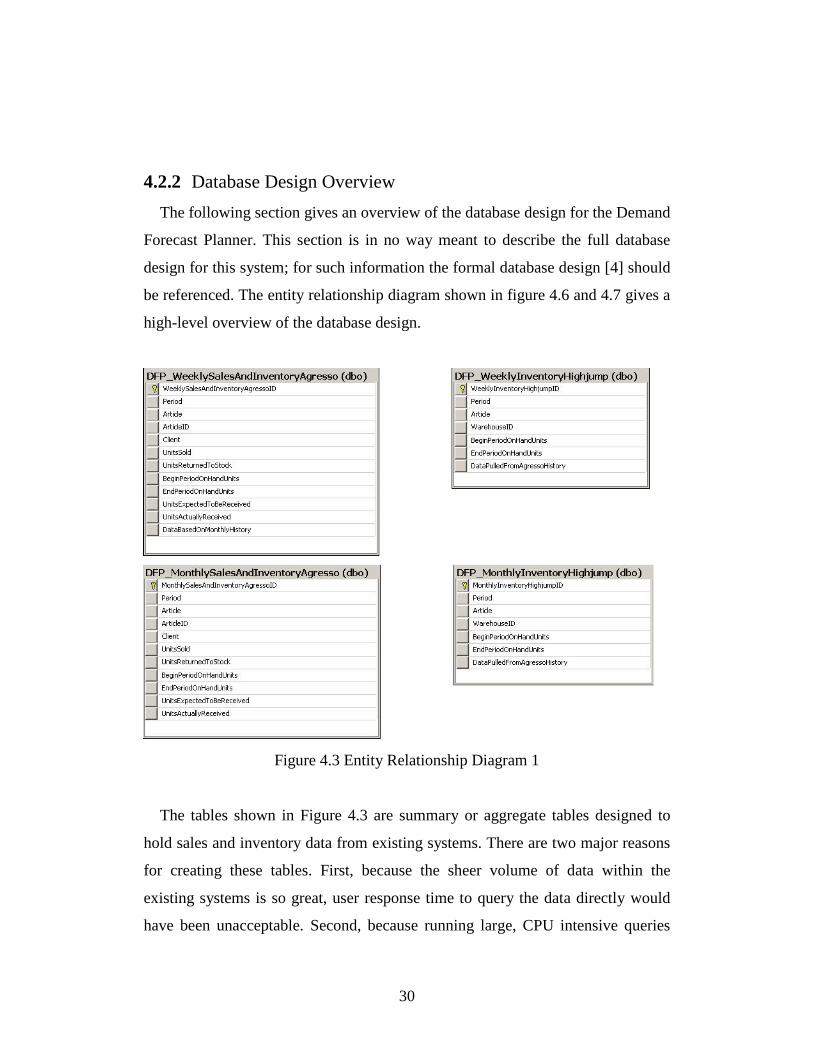
4.2.2 Database Design Overview
The following section gives an overview of the database design for the Demand
Forecast Planner. This section is in no way meant to describe the full database
design for this system; for such information the formal database design [4] should
be referenced. The entity relationship diagram shown in figure 4.6 and 4.7 gives a
high-level overview of the database design.
Figure 4.3 Entity Relationship Diagram 1
The tables shown in Figure 4.3 are summary or aggregate tables designed to
hold sales and inventory data from existing systems. There are two major reasons
for creating these tables. First, because the sheer volume of data within the
existing systems is so great, user response time to query the data directly would
have been unacceptable. Second, because running large, CPU intensive queries

31
throughout the day would have adversely affected the performance of the existing
systems. For these reasons, a set of views and stored procedures were created and
scheduled to be ran during off peak hours to load these summary tables that the
Demand Forecast Planner would then use in place of running queries directly
against the existing systems. Data could potentially become as much as one day
out of sync with the existing systems, but this is considered an acceptable tradeoff
for increased performance.
Figure 4.4 Entity Relationship Diagram 2
The DFP_ForecastWarehouse table in Figure 4.4 is designed to support the
ForecastWarehouse class from the class design. This table includes a name and ID

32
that represent a physical warehouse. Using a primary/foreign key relation with
DFP_ForecastWarehouseHighjumpWarehouse and
DFP_ForecastWarehouseClient tables these tables show the particular data in
existing systems that should be combined to define a ForecastWarehouse entity.
The DFP_ForecastWarehouseTransfer table represents the acceptable types of
inter-warehouse transfers. For example, this table specifies if inventory can be
transferred from the U.S. warehouse to the Mexico warehouse and vice versa. The
last table that represents data associated with the ForecastWarehouse class is the
DFP_WarehouseProdutPeriodTransfer table. This table represents an actual
transfer from one warehouse to another. It specifies the product being transferred,
the source and destination warehouse, the number of units being transferred and
the period of time when the units are transferred.
The DFP_WarehouseProduct table shown in Figure 4.4 was designed to
support the WarehouseProduct class required in the class design. This table
represents a relationship between a warehouse and a product, using a
primary/foreign key relation with DFP_WarehouseProductPeriodUserData,
projected future sales, and inventory levels for a given WarehouseProduct can be
represented.
Lastly the table DFP_ProductProfile defined in Figure 4.4 is designed to
support the ProductProfile class from the class design. This table represents a
relationship between two WarehouseProduct entities or a single
WarehouseProduct entity and a product line. This data is used to substitute
historical sales and inventory data from one WarehouseProduct, or product line,
to another WarehouseProduct that does not have enough historical data to predict
future inventory needs.
4.3 Lessons Learned During Design
This section will detail some of the major areas that the Development Team
believes could be improved or that played an especially important role in the

33
design phase. A problem that arose both in the requirements phase and the design
phase was a lack of tool support. While tools are available to model both the class
and database design, Microsoft Word was again used to specify the detailed class
and database designs. The increased amount of data tracked in the design phase,
as compared to the requirements phase, made the design documents cluttered and
hard to navigate. With the class and database design each extending beyond fifty
pages, finding key design decisions became cumbersome.
A tool that allows both modeling capabilities and additional detailed design
support would have been helpful to the Development Team. A way to track
collaboration on design decisions would help outside parties understand the
thought process that went into the design. The collaboration that went into design
decisions for the Demand Forecast Planner was omitted by the Development
Team from the detailed design documents in many cases to keep these documents
a manageable size. Along with this concept, a way of tracking versions of design
documents could have been useful.
Tool support to help navigate the detailed design documents would also have
been beneficial. A way of sorting and filtering a design specification based on
phase or a user defined logical category could increase the efficiency in the
Development Team’s ability to access key design information. Because class and
database design are closely related, tools linking the two areas of design were
needed. Overall tool support rather than free form text could greatly increase the
effectiveness of the Development Team during the design phase.
Another important lesson learned during the design phase was how important a
well defined class design is for understanding and further designing a system.
Refining requirements into small, easily understandable units greatly helped the
Development Team’s understanding of the problem. Additionally, abstracting the
data into classes made the database design a straight forward task of supporting
the underlying classes; this simplified design. The upfront time invested in

34
properly creating the classes for the Demand Forecast Planner was the key to the
Development Team’s success.

35
5. Implementation
The third phase of software development is the implementation or coding
phase. IEEE has the following definition for coding [6].
“
1. In software engineering, the process of expressing a computer program
in a programming language.
2. (IEEE Std 1002-1987) The transforming of logic and data from design
specifications (design descriptions) into a programming language.
”
Unlike the requirements gathering and design phases, the implementation phase
should not require a great deal of upfront time. Most of the consideration on how
the system will be created was done in the design phase and actually
implementing the system at this point should be a mechanical translation from
design to code. If excessive time is required during implementation, then it is
likely the design is inadequate and needs further work. The reason so much time
was spent in the requirements gathering and design phases was to make the
implementation phase simple and straight forward.
5.1 Implementing the Demand Forecast Planner While no official methodology was followed during the implementation of the
Demand Forecast Planner, a number of guidelines were followed by the
Development Team that applied to this phase. This section will give a brief
overview of the implementation guidelines followed, but little detail will be given
to the actual code itself as this is outside the scope of this document. Table 5.1
lists several of the most important guidelines and best practices related to
variables used during this phase.
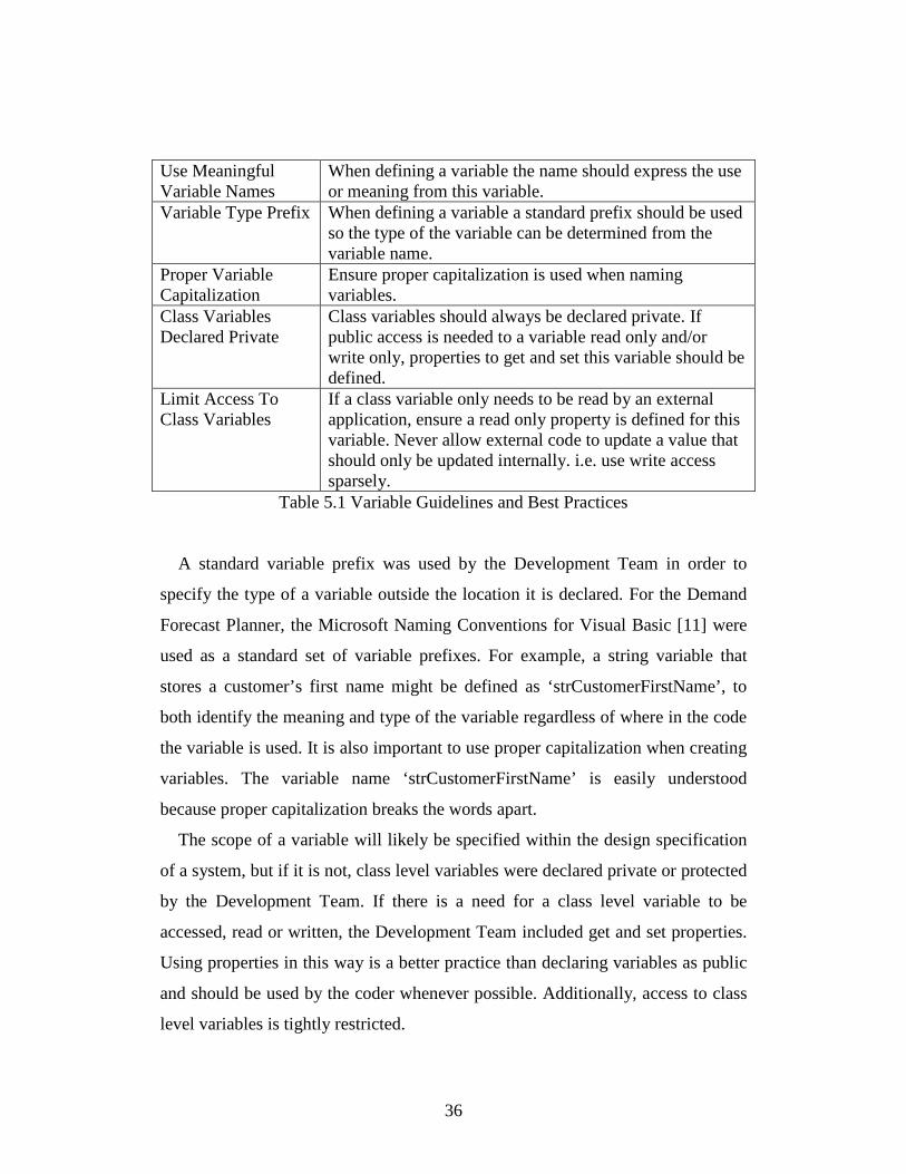
Coding Guideline Guideline Description
36
Use Meaningful Variable Names
When defining a variable the name should express the use or meaning from this variable.
Variable Type Prefix When defining a variable a standard prefix should be used so the type of the variable can be determined from the variable name.
Proper Variable Capitalization
Ensure proper capitalization is used when naming variables.
Class Variables Declared Private
Class variables should always be declared private. If public access is needed to a variable read only and/or write only, properties to get and set this variable should be defined.
Limit Access To Class Variables
If a class variable only needs to be read by an external application, ensure a read only property is defined for this variable. Never allow external code to update a value that should only be updated internally. i.e. use write access sparsely.
Table 5.1 Variable Guidelines and Best Practices
A standard variable prefix was used by the Development Team in order to
specify the type of a variable outside the location it is declared. For the Demand
Forecast Planner, the Microsoft Naming Conventions for Visual Basic [11] were
used as a standard set of variable prefixes. For example, a string variable that
stores a customer’s first name might be defined as ‘strCustomerFirstName’, to
both identify the meaning and type of the variable regardless of where in the code
the variable is used. It is also important to use proper capitalization when creating
variables. The variable name ‘strCustomerFirstName’ is easily understood
because proper capitalization breaks the words apart.
The scope of a variable will likely be specified within the design specification
of a system, but if it is not, class level variables were declared private or protected
by the Development Team. If there is a need for a class level variable to be
accessed, read or written, the Development Team included get and set properties.
Using properties in this way is a better practice than declaring variables as public
and should be used by the coder whenever possible. Additionally, access to class
level variables is tightly restricted.

37
Another important area that needs to be focused on during the implementation
phase is readability, complexity and understandability of code. Table 5.2 defines
several of the most important guidelines and best practices related to these areas
that were used by the Development Team while implementing the Demand
Forecast Planner.
Coding Guideline Guideline Description
Commenting and Standard Comment Blocks
Commenting code is an important part of coding and should be done consistently, using a standard comment style or built in language specific comment block if supported.
Regions and Logical Groupings
Logically grouping like segments of code should be done to increase readability and understandability. Regions should be used if supported by the language being used.
Complex Functions Broken Apart if Possible.
Whenever possible, large and complex functions should be broken out into smaller and easer to understand functions. This will help readability, complexity and understandability of the code.
Table 5.2 Readability, Complexity and Understandability Guidelines
Commenting code is an elementary concept in software engineering and
properly writing code, but one that is often overlooked. To help with the task of
commenting code the Development Team used Microsoft Visual Studio’s
standard comment block. The use of these standard comment blocks (illustrated in
figure 5.3) can help to clearly define the code. Additionally third party tool
support is available for converting these standard comment blocks into auto
generated help files or online documentation. While this topic is interesting, this
document will not discuss the use of such auto generating help file tools, but more
information on this topic can be obtained from [12].
38
Figure 5.3 Standard Comment Block
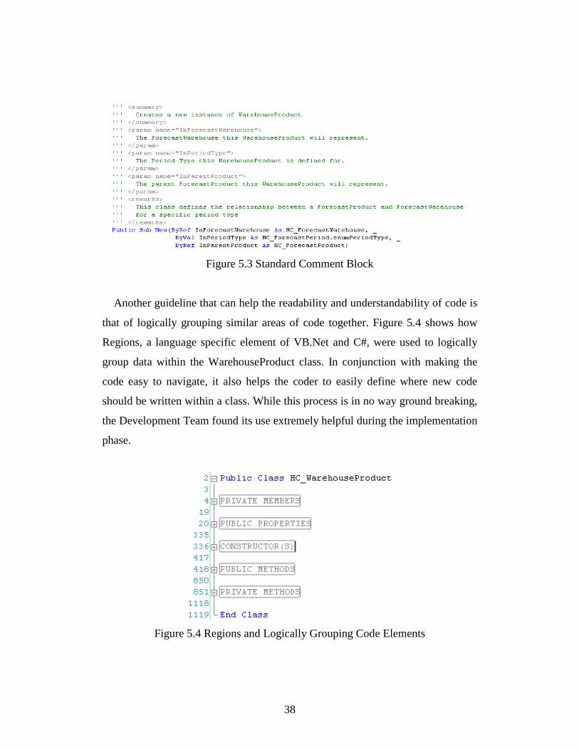
Another guideline that can help the readability and understandability of code is
that of logically grouping similar areas of code together. Figure 5.4 shows how
Regions, a language specific element of VB.Net and C#, were used to logically
group data within the WarehouseProduct class. In conjunction with making the
code easy to navigate, it also helps the coder to easily define where new code
should be written within a class. While this process is in no way ground breaking,
the Development Team found its use extremely helpful during the implementation
phase.
Figure 5.4 Regions and Logically Grouping Code Elements

39
The complexity of functions should be reviewed and specified within the
design phase, but sometimes what seems simple during the design may become
more complex when coding begins. If this happens during the implementation
phase, the design should be updated and reviewed to ensure the change will not
affect the rest of the software system.
The last set of guidelines used by the Demand Forecast Planner that will be
discussed is that of error handling and using built-in libraries. Table 5.6 defines
two important guidelines and best practices related to these areas.
Coding Guideline Guideline Description
All Code Within A Try Catch Block
Any code that has the potential to cause an error should be defined with a Try Catch block to handle potential exceptions.
Do not Reinvent the Wheel – Use Libraries
The libraries of frameworks of commercial software packages today are extensive and likely have already solved a majority of the problems that will be encountered while coding.
Table 5.6 Error Handling and Library Usage Guidelines
Proper error handling can help to pinpoint errors and quickly identify how to
correct them. For this reason, the Development Team placed the majority of code
written within try catch blocks. The Development Team also strove to attend to
software reuse whenever possible. For example the design for the Demand
Forecast Planner required that the ICompariable interface be implemented to sort
sales and inventory data by period. The use of this interface allowed the
Development Team to take advantage of library specific data structures to store
and sort custom objects.
5.2 Code Metrics for the Demand Forecast Planner At the time of its initial release the Demand Forecast Planner consists of eight
classes. These eight classes include a total of forty-two public methods for an
average of approximately five public methods per class. The total lines of code
40
contained within these eight classes is 4,954, and the total lines for code for the
complete application, classes and GUI, is 6,279. While these numbers might seem
small for an application of this size, the database objects needed to support the
Demand Forecast Planner were complex and offloaded a large amount of work to
the database.
The supporting database contains twenty-one tables. Additionally, thirty-two
stored procedures and eight views were created to support the retrieval of data for
the application. Lastly, two scheduled SQL jobs were created to aggregate data
from existing systems to ensure adequate performance for the Demand Forecast
Planner. The total lines of code for the above database objects totals 1,863.

41
6. Testing
The fourth phase of software development is the testing phase. IEEE has the
following definition for testing [6].
“
1. An activity in which a system or component is executed under specified
conditions, the results are observed or recorded, and an evaluation is
made of some aspect of the system or component.
2. To conduct an activity as in (1).
”
In the context of the Demand Forecast Planner this definition refers to executing a
specific area of the application with an expected output, and then comparing the
actual output to what was expected. A specific test, or test case, should be derived
from the requirements, as the purpose of every test should be to verify the system
or component is doing what it is required to do. Creating test cases before the
design and implementation phases begin will often lead to a more complete
design and less errors within the code.
6.1 Testing Methodology To test the Demand Forecast Planner, a methodology loosely based on the
IEEE 829-1998 standard [9] for software testing documentation was used. This
standard was mainly used by the Development Team to specify a set of test cases
to verify the Demand Forecast Planner adhered to the requirements specified for
the system. These test cases were used to conduct system testing before the
application was turned over to end users for user acceptance testing.
User acceptance testing was used to validate that the Demand Forecast Planner
met the requirements of its end users. While the Development Team learned a
great deal about the purchasing and manufacturing areas of the business during
the development of the Demand Forecast Planner, in the end the Development

42
Team members are not purchasing professionals and were unable to determine if
the application would be adequate to meet the purchasing needs of its end users.
6.2 Testing the Demand Forecast Planner The following section gives an overview of the testing phase for the Demand
Forecast Planner. During this phase, the Development Team first produced a set
of generic test cases based on the requirements created in the first step of the
software life cycle. These test cases did not use application domain specific data,
but rather generic sample data used to illustrate how the final system should
function. These generic test cases were translated into application domain specific
test cases when the application was complete and testing began. Table 6.1 is the
set generic test data and test cases that were defined for the Demand Forecast
Planner; for additional information the formal test plan [5] should be referenced.
Sample Data for Fictional Product TST01 – US Warehouse
Period
TY Plan Sls
PY Sls
PY Plan Sls
PPY Sls
TY BoH
TY EoH
PY BoH
PY EoH
Plan On
Order
Actual On
Order 200801 300 150 135 20 2222 1922 2000 1850 0 0 200802 303 153 138 23 1922 1619 1850 1697 0 0 200803 306 156 140 26 1619 1313 1697 1541 0 0 200804 309 159 143 29 1313 1004 1541 1882 0 0 200805 312 162 146 32 1004 692 1882 1720 0 0 200806 315 165 149 35 692 377 1720 1555 0 0 200807 318 168 151 38 377 2059 1555 1387 0 2000 200808 321 171 154 41 2059 1738 1387 1216 0 0 200809 324 174 157 44 1738 1414 1216 1042 0 0 200810 327 177 159 47 1414 1087 1042 865 0 0 200811 330 180 162 50 1087 757 865 685 0 0 200812 333 183 165 53 757 2424 685 502 0 2000 200813 336 186 167 56 2424 2088 502 316 0 0 200814 339 189 170 59 2088 1749 316 127 0 0 200815 342 192 173 62 1749 1407 127 935 0 0 200816 345 195 176 65 1407 1062 935 740 0 0
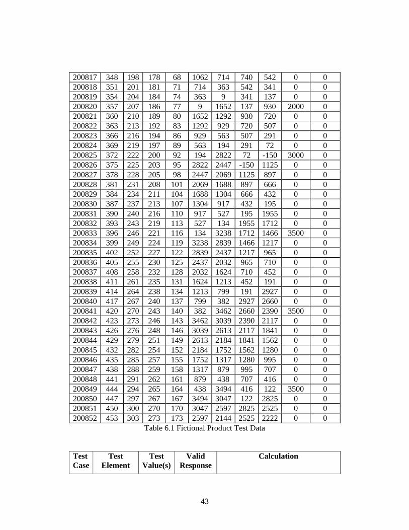
43
200817 348 198 178 68 1062 714 740 542 0 0 200818 351 201 181 71 714 363 542 341 0 0 200819 354 204 184 74 363 9 341 137 0 0 200820 357 207 186 77 9 1652 137 930 2000 0 200821 360 210 189 80 1652 1292 930 720 0 0 200822 363 213 192 83 1292 929 720 507 0 0 200823 366 216 194 86 929 563 507 291 0 0 200824 369 219 197 89 563 194 291 72 0 0 200825 372 222 200 92 194 2822 72 -150 3000 0 200826 375 225 203 95 2822 2447 -150 1125 0 0 200827 378 228 205 98 2447 2069 1125 897 0 0 200828 381 231 208 101 2069 1688 897 666 0 0 200829 384 234 211 104 1688 1304 666 432 0 0 200830 387 237 213 107 1304 917 432 195 0 0 200831 390 240 216 110 917 527 195 1955 0 0 200832 393 243 219 113 527 134 1955 1712 0 0 200833 396 246 221 116 134 3238 1712 1466 3500 0 200834 399 249 224 119 3238 2839 1466 1217 0 0 200835 402 252 227 122 2839 2437 1217 965 0 0 200836 405 255 230 125 2437 2032 965 710 0 0 200837 408 258 232 128 2032 1624 710 452 0 0 200838 411 261 235 131 1624 1213 452 191 0 0 200839 414 264 238 134 1213 799 191 2927 0 0 200840 417 267 240 137 799 382 2927 2660 0 0 200841 420 270 243 140 382 3462 2660 2390 3500 0 200842 423 273 246 143 3462 3039 2390 2117 0 0 200843 426 276 248 146 3039 2613 2117 1841 0 0 200844 429 279 251 149 2613 2184 1841 1562 0 0 200845 432 282 254 152 2184 1752 1562 1280 0 0 200846 435 285 257 155 1752 1317 1280 995 0 0 200847 438 288 259 158 1317 879 995 707 0 0 200848 441 291 262 161 879 438 707 416 0 0 200849 444 294 265 164 438 3494 416 122 3500 0 200850 447 297 267 167 3494 3047 122 2825 0 0 200851 450 300 270 170 3047 2597 2825 2525 0 0 200852 453 303 273 173 2597 2144 2525 2222 0 0
Table 6.1 Fictional Product Test Data
Test Case
Test Element
Test Value(s)
Valid Response
Calculation

44
1 Avg Inventory
TST01 1575 BOH Qty for the future 52 weeks / 52.
2 52 Week Projected
Sales
TST01 19578
Sum of this year’s planned sales (TY PLAN SLS) for the next 52
weeks.
3 PY 52 Week Sales
TST01 11778 Sum of last year’s sales (PY SLS) 52 weeks.
4 Avg Weekly Sls
Units
TST01 377 Sum of this year’s planned sales (TY PLAN SLS) for the next 52
weeks divided by 52.
5 12 Week Avg Sls
Units
TST01 317 Sum of this year’s planned sales (TY PLAN SLS) for the next 12
weeks divided by 12.
6 Total Units On Order
TST01 4000 Total units for a particular item that are on existing, approved purchase
orders.
7 PPY Sls TST01
200805
32 None
8 PY Sls TST01
200805
162 None
9 PY Sls As % PPY Sls
TST01
200805
406.25% (PY Sales/PPY Sales) – 1
10 PY Sls As % PY Plan
Sls
TST01
200805
10.95% (PY Sales/PY Plan Sls) – 1
11 PY Plan Sls
TST01
200805
146 None
12 PY Plan Sls As % PY Sls
TST01
200805
-9.87% (PY Plan Sls/PY Sales) – 1
13 TY Plan Sls
TST01
200805
312 None
14 TY Plan Sls As % PY Sls
TST01
200805
92.59% (TY Sales/PY Sales) – 1
(USER INPUT)

45
15 PY BOP TST01
200805
1882 None
16 PY EOP TST01
200805
1720 None
17 PY Turn TST01
200805
8.99% (PY SLS) / ( ((PY BOP) + (PY EOP))/2 )
18 TY Act/Plan
BOP
TST01
200805
1004 For current period no calculations just get current BOP units.
For future periods retrieve the
previous periods TY Plan EOP.
19 TY Plan EOP
TST01
200805
692 (TY Act/Plan BOP) + (Actual On Order) + (Plan On Order) – (TY
PLAN SLS) 20 TY Plan
Turn TST01
200805
36.79% (TY PLAN SLS) / (((TY Act/Plan BOP) + (TY Plan EOP)) / 2)
21 TY Periods TST01
200805
2.09 (TY Plan EOP) / (Sum Next 12 Periods TY PLAN SLS / 12)
22 PY Received
TST01
200805
0 None
23 Plan On Order
TST01
200805
0 None
24 Actual On Order
TST01
200805
0 None
Table 6.2 Test Cases for Fictional Product TST01
The data in Tables 6.1 and 6.2 does not completely cover all requirements for
the Demand Forecast Planner, but the Development Team believes these test
cases encompass the major functionality. While all the data used for the above test
cases is fictional, it clearly illustrates how the final system should function. The
above test cases were created by the Development Team, but signed off by the
customer to ensure both sides were in agreement as to what needed to be

46
delivered in the end product. This open dialog was helpful to the Development
Team and led to a few updates to the initial requirements.
Although these test cases did not test data for an actual product, they defined
what would be tested in the final system. After the design and implementation
phases were complete, these generic test cases were translated into specific test
cases for the final system. This decreased the amount of time needed to test the
system once it was complete, as well as made the testing process a fairly
mechanical process of plugging in numbers and looking for an expected result.
The following is the set of specific test cases defined after the implementation
phase was complete.
Actual Data for Product CO6323 (9 Ply, 10 Piece Set) – US Warehouse
Period TY Sls
PY Sls
PY Pln Sls
PPY Sls
TY BoH
TY EoH
PY BoH
PY EoH
Plan On
Order
Actual On
Order 200838 93 155 0 228 218 125 4468 4337 0 0 200839 62 103 0 217 125 63 4315 4185 0 0 200840 97 162 0 199 63 -34 4163 4032 0 0 200841 98 164 0 267 -34 -132 4010 3880 0 0 200842 73 122 0 157 -132 -205 3858 3747 0 0 200843 79 132 0 186 -205 -284 3728 3618 0 0 200844 72 120 0 264 -284 -356 3599 3488 0 0 200845 86 144 0 382 -356 -442 3470 3358 0 0 200846 95 158 0 193 -442 -537 3358 3185 0 0 200847 66 110 0 200 -537 -603 3185 3078 0 0 200848 74 124 0 228 -603 -677 3078 2961 0 0 200849 74 124 0 243 -677 249 2961 2844 1000 0 200850 116 194 0 198 249 133 2844 2661 0 0 200851 50 84 0 219 133 83 2661 2563 0 0 200852 76 126 0 209 83 7 2563 2440 0 0 200901 97 162 0 157 7 -90 2440 2307 0 0 200902 52 86 0 351 -90 -142 2307 2210 0 0 200903 107 178 0 183 -142 -249 2210 2041 0 0 200904 113 188 0 197 -249 -362 2041 1901 0 0 200905 86 143 0 211 -362 -448 1901 1688 0 0 200906 70 117 0 123 -448 -518 1688 1634 0 0

47
200907 6 6 0 130 -518 -524 1564 0 0 0 200908 57 57 0 120 -524 -581 0 1504 0 0 200909 98 98 0 211 -581 -279 1504 670 400 0 200910 111 111 0 204 -279 -390 670 561 0 0 200911 113 113 0 226 -390 -503 561 449 0 0 200912 89 89 0 206 -503 -592 449 1016 0 0 200913 126 126 0 228 -592 -718 1016 928 0 0 200914 109 109 0 211 -718 -827 928 847 0 0 200915 131 131 0 220 -827 -958 847 752 0 0 200916 145 145 0 233 -958 -1103 752 599 0 0 200917 105 105 0 204 -1103 -1208 599 512 0 0 200918 96 96 0 227 -1208 -1304 512 401 0 0 200919 90 90 0 207 -1304 -1394 401 316 0 0 200920 130 130 0 199 -1394 -1524 316 185 0 0 200921 92 92 0 206 -1524 -1116 185 87 500 0 200922 82 82 0 197 -1116 -1198 87 0 0 0 200923 122 122 0 179 -1198 -1320 120 0 0 0 200924 113 113 0 204 -1320 -1433 0 101 0 0 200925 163 163 0 166 -1433 -596 101 92 1000 0 200926 108 108 0 169 -596 -704 92 388 0 0 200927 83 83 0 158 -704 -787 388 517 0 0 200928 95 95 0 176 -787 -882 517 558 0 0 200929 105 105 0 139 -882 -987 558 476 0 0 200930 81 81 0 172 -987 -1068 476 397 0 0 200931 110 110 0 111 -1068 -1178 397 300 0 0 200932 82 82 0 197 -1178 -1260 300 216 0 0 200933 61 61 0 155 -1260 -1321 216 141 0 0 200934 62 62 0 120 -1321 -1383 141 144 0 0 200935 75 75 0 124 -1383 -1458 144 214 0 0 200936 81 81 0 165 -1458 -1539 214 199 0 0 200937 90 90 0 225 -1539 -1629 199 233 0 0
Table 6.3 Product Data for CO6323 (9 Ply, 10 Piece Cookware Set)
Test Case
Test Element
Test Value(s)
Valid Response
Calculation Test Case
1 Avg Inventory
CO6323 -660 -660 Pass
2 52 Week Projected
Sales
CO6323 4747 4747 Pass

48
3 PY 52 Week Sales
CO6323 5907 5907 Pass
4 Avg Weekly Sls
Units
CO6323 91 91 Pass
5 12 Week Avg Sls
Units
CO6323 80 80 Pass
6 Total Units On Order
CO6323 0 2900 Fail
Don’t Include Planned
On Order
7 PPY Sls CO6323
200850
198 198 Pass
8 PY Sls CO6323
200850
194 194 Pass
9 PY Sls As % PPY Sls
CO6323
200850
-2% -2% Pass
10 PY Sls As % PY Plan
Sls
CO6323
200850
0% 0% Pass
11 PY Plan Sls CO6323
200850
0 0 Pass
12 PY Plan Sls As % PY
Sls
CO6323
200850
0 0 Pass
13 TY Plan Sls CO6323
200850
116 116 Pass
14 TY Plan Sls As % PY
Sls
CO6323
200850
-40% -40% User Input
15 PY BOP CO6323
200850
2844 2844 Pass
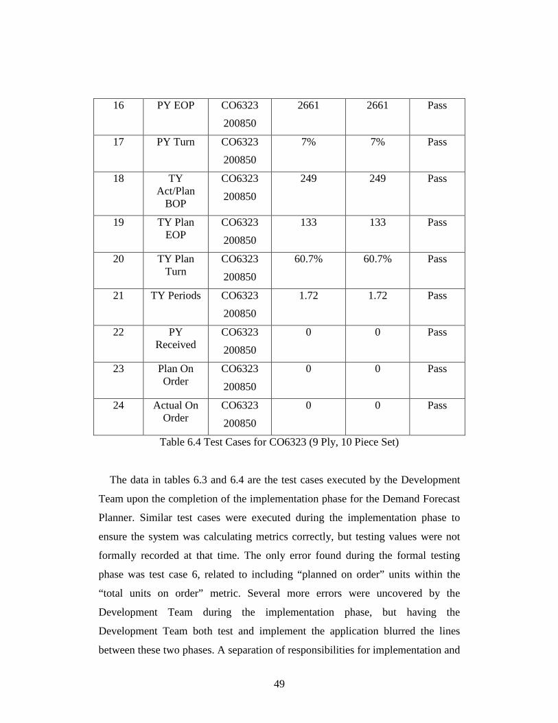
49
16 PY EOP CO6323
200850
2661 2661 Pass
17 PY Turn CO6323
200850
7% 7% Pass
18 TY Act/Plan
BOP
CO6323
200850
249 249 Pass
19 TY Plan EOP
CO6323
200850
133 133 Pass
20 TY Plan Turn
CO6323
200850
60.7% 60.7% Pass
21 TY Periods CO6323
200850
1.72 1.72 Pass
22 PY Received
CO6323
200850
0 0 Pass
23 Plan On Order
CO6323
200850
0 0 Pass
24 Actual On Order
CO6323
200850
0 0 Pass
Table 6.4 Test Cases for CO6323 (9 Ply, 10 Piece Set)
The data in tables 6.3 and 6.4 are the test cases executed by the Development
Team upon the completion of the implementation phase for the Demand Forecast
Planner. Similar test cases were executed during the implementation phase to
ensure the system was calculating metrics correctly, but testing values were not
formally recorded at that time. The only error found during the formal testing
phase was test case 6, related to including “planned on order” units within the
“total units on order” metric. Several more errors were uncovered by the
Development Team during the implementation phase, but having the
Development Team both test and implement the application blurred the lines
between these two phases. A separation of responsibilities for implementation and

50
testing the Demand Forecast Planner would have likely resulted in a higher
quality and more error-free initial release. The reality of the situation, and that of
many in-house applications, was that the Development Team was required to both
implement and test the application. The Development Team would have preferred
the help of a separate testing team, but as none was available, initial testing was
conducted by the Development Team and user acceptance testing was heavily
used to find any additional errors.
Lastly, user acceptance testing was conducted to ensure the Demand Forecast
Planner met the initially defined requirements of the system and to uncover any
errors not detected within the formal testing phase. During this phase the
Development Team met with the customer and recorded feedback about the
system. While the customer used the application, a few errors were uncovered as
well as a few enhancement requests for functionality not initially defined within
the requirements. Errors were recorded and corrected by the Development Team
while enhancement requests were incorporated into the requirements and design
and added to the system. After a few iterations of this process, the system was
officially released based on the acceptance of the customer.
6.3 Lessons Learned During Testing
This section will detail some of the major areas that the Development Team
feels could have been improved or played an especially important roll during the
testing phase. One of the major struggles during the testing phase was that the
same personnel served as coding and testing groups. While having the same group
both code and test the system does not mean a quality system can not be
delivered, it is generally better to have these tasks preformed by separate groups.
Generally, the coding group is unlikely to give the same level of detailed testing
as an independent testing group. This was true in the testing of the Demand
Forecast Planner and lead to a few faults being identified during user acceptance
testing rather than during system test.

51
Another issue that was not specific to the testing phase, but affected the testing
phase more than any other, was the high demand for the system to be available as
quickly as possible. Given a limited amount of time to develop the system, a great
deal of formal testing was delayed until user acceptance testing. Had the testing
phase been given more time, more of these issues could have been found prior to
user acceptance testing.
The close proximity of the Development Team and customer proved to be
helpful for testing the Demand Forecast Planner. This made it easy to get
feedback quickly and facilitated user acceptance testing. The Development Team
could correct an issue and then walk over to the customer and see the effects of
that change, getting quick feedback from the customer. This efficient dialog
helped to ensure the system was functioning as required and pinpoint any errors
quickly.

52
7. Maintenance The fifth, and normally final phase of software development, is the
maintenance phase. IEEE has the following definition for maintenance [6].
“
1. Software maintenance is the process of modifying a software system or
component after delivery to correct faults, improve performances or
other attributes, or adapt to a changed environment.
2. The process of retaining a hardware system or component in, or
restoring it to, a state in which it can perform its required functions.
”
In the context of the Demand Forecast Planner the maintenance phase started
before the system was delivered. While the official definition states maintenance
is a task that occurs after delivery, the Development Team started putting a
maintenance framework in place throughout the software life cycle. This
maintenance framework helped facilitate the task of maintaining the Demand
Forecast Planner after its initial release.
7.1 Maintenance Methodology
No formal methodology was followed to support the maintenance activities of
the Demand Forecast Planner. The activity of maintaining a software system is
really just repeating the requirements, design, coding and testing phases of the
software life cycle for an existing system. For this reason, the Development
Team’s major goal was to incorporate maintenance elements into these phases to
help support any future changes. In the requirements phase these maintenance
elements would help to define when a specific requirement was defined for the
system as well as if a requirement was changed from one release to another, and
how the requirement was changed. This tracking of requirements to a specific
release gives a road map of system change from release to release. The tracking

53
also assists in maintaining the same strict software development practices when
developing future requirements.
Design element introduction was also tracked. This gave a clear understanding
of how the design changed over time. The goal of this approach was to keep
maintenance changes from bypassing the requirements and design phases. While
this might be acceptable for correcting coding issues, most changes to an existing
system should update the corresponding requirements and design of the system so
an accurate representation of the working system can be identified from the
requirements and design.
Adequate commenting, including date and reason a change was made, is the
first major maintenance element the Development Team used within the
implementation phase. Additionally, a number of different programmers will be
working on the system over its lifetime, and including who made a specific
change was added to comments while maintaining the code. While source code
control is not exactly an element that would be added to the code to facilitate
maintenance, it was also used during the coding and maintenance phases. For the
Development Team knowing exactly what was changed and when was helpful in
identifying newly introduced bugs that were the result of a maintenance task.
7.2 Maintaining the Demand Forecast Planner There has not yet been sufficient time to perform much maintenance on the
Demand Forecast Planner. To illustrate how maintenance is planned to be
performed, this section will follow the first change request from initial request
through implementation and testing. It is expected that this process will be
continued for future enhancements and/or error fixes.
The first step in the maintenance phase was for the Development Team to
document enhancements and/or errors. Figure 6.1 is an excerpt of the meeting
minutes between the Development Team and the customer requesting new
functionality. This request provides a description of the change request as given

54
by the customer and will be referenced when updating the requirements, design,
code and test plan of the Demand Forecast Planner.
Figure 7.1 First Enhancement Request
With the change request documented, the next step was for the Development
Team to update the requirements to include the newly requested functionality. In
order to assist the Development Team in tracking a change request back to the
requirements the date of the change request was used as a reference. While this
reference is not the best solution, for small single-person projects it works fairly
effectively. A better solution would have been to track the change request within a
help desk style of software and then use the ID from this system as a reference.
Table 7.2 and figure 7.3 show the updates made to the software requirement
specification [2] for the change request. The “Date/Phase Added” element
captures what and when this change was applied, and the date can be used to
reference the original change request to explain why the change was made.

55
Period Based Purchasing Terms For Sales Term Definition Calculation/Reference Date/Phase
PY Wrnty Sls Prior year warranty sales.
None 11/20/2008 – User Testing Round 1
PY Wrnty Sls As % PY Sls
Prior year’s warranty sales expressed as a % +/- prior year’s sales.
PY Wrnty Sls/PY Sales 11/20/2008 – User Testing Round 1
Table 7.2 Updated Terms for Change Request
Figure 7.3 Updated Requirements for Change Request
The next step completed by the Development Team to implement this change
request was to update the design. The process of reviewing the design, along with
an initial design that was laid out with expansion in mind, helped the
Development Team easily pinpoint the location the proposed change would fit
best. Thinking of how best to incorporate this change into the design, rather than
jumping directly to the code, not only made the change fit better into the overall
application, but also kept the software development life cycle documentation up-
to-date with the system. Figure 7.4 shows the sections of the class design [3]
updated for this change request. The Development Team again used the date of
the change request to indicate when and what was changed. The database design

56
was also updated, but because of the complex SQL involved, the changes are not
shown here; please refer to [4] for more information.
Figure 7.4 Updated Class Design for Change Request
With a good design and supporting requirements in place, the next step for the
Development Team was to actually change the source code. Given the careful
requirements and design efforts, making changes to the code became a fairly
mechanical process of translating the design into code. To track the changes, the
Development Team added comments to specify who was making the change,
when the change was made and why the change was made. Figure 7.5 shows one
of the source code changes made and the commenting that accompanied the
change..

57
Figure 7.5 Updated Source Code for Change Request
A source code control application called Vault was used by the Development
Team to keep track of any changes made to the source code. Source code control
will track every change made to the source code as well as who made it and when
it was made. Source code control will version each committed change to the
source code and these versions can easily be rolled back or promoted if needed.
Built-in tools also make comparing two different versions of source code easy.
Figure 7.6 shows one area of the source code before and after the change request
was implemented. With this change request, the code did not exist at all in the
previous version of the system, but had the request been to change a calculation
within an existing class element, source code control can be extremely helpful in
identifying what was change from one version to the next.
Figure 7.6 Source Code Control Comparison

58
The last maintenance task completed by the Development Team was to update
the test plan to include a test case to test the requested change. This test plan was
then executed to ensure the new change worked correctly, as well as to perform
regression testing to ensure none of the previously working areas of the
application stopped working. For more information on the test cases executed for
the change request discussed in this section, see the formal test plan [5].
7.3 Lessons Learned During Maintenance The maintenance phase of the Demand Forecast Planner is just beginning, but
the Development Team has already learned a number of lessons during the initial
maintenance request. This section will detail a few of the areas important to the
maintenance of this system, as well as some areas important to the general
maintenance phase of software that will be used going forward. One of the most
useful steps taken by the Development Team to support the Demand Forecast
Planner was to have the supporting documentation, such as requirements, design
and testing grow with the application. On past projects, the Development Team
has seen these documents initially created, but only the source code modified as
the application required changes or enhancements. This reactionary maintenance,
rather than planned maintenance, led to applications being disjoint from their
initial design and difficult to maintain over time.
Additionally, having the ability to track a maintenance request from the initial
request through implementation and testing of that request is was found to be
useful by the Development Team. Knowing when and why the system changed
was many times as important as the change itself. The use of maintenance
elements within the software life cycle documents and code worked well for the
Development Team to track this information. Moving forward with the
maintenance process, it might become necessary to create separate versions of the
software life cycle documents if a major change is introduced to the system. As

59
noted in the requirements and design phases, proper tool support would likely also
ease the process of maintaining software life cycle documents.

60
8. The Demand Forecast Planner Application
This section will give an overview of the Demand Forecast Planner application
that was created as a result of the software development processes described in
this document. This section will not detail every feature of the Demand Forecast
Planner, but will detail the most important areas of the application.
Figure 8.1 Product Selection Form
The Product Selection Form, shown in figure 8.1, is a form that allows the user
to select a product to forecast. A vendor drop down was added to assist the user
by narrowing the product search down to products supplied by a specific vendor.
Additionally, two radio buttons were added to assist the user in filtering out active
products that are currently for sales from products that are no longer sold.

61
Figure 8.2 Demand Forecast Planner Form (Summary and Sales Information)

62
Figure 8.3 Demand Forecast Planner Form (Inventory Information)
Figure 8.2 shows the half of the Demand Forecast Planner Form that displays
summary and sales information. Figure 8.3 shows the half of the Demand
Forecast Planner Form that displays inventory information. Figures 8.2 and 8.3
would normally span one row, but are broken apart for visibility. The upper left
63
corner of figure 8.2 displays a color key that indicates if the data in a specific
column is pulled from the system database, calculated based on a formula or a
user entered value. Directly under this color key is summary information about
the specific WarehouseProduct that is being viewed. The WarehouseProduct can
be changed by selecting a different warehouse tab. The two warehouses “WH_1
(US)” and “WH_2 (MX)” can be seen as tabs across the top of Figure 8.2.
The grid shown in Figures 8.2 and 8.3 shows a set of past, present and future
sales and inventory information for the selected WarehouseProduct. The first
column in Figure 8.2 displays the weekly period from the current week to one
year in the future where the first row is the current week and the last row is one
year from the current week. The columns to the right of the weekly period column
show the sales and inventory information during that period of time. Each row is
bound to a PeriodSalesAndInventoryData object as described in the class design
section 4.2.1 that holds the specific sales and inventory information for that period
of time.
When the yellow, user input, column values are changed the system updates the
underlying PeriodSalesAndInventoryData object corresponding to that row and
the forecasted future sales and inventory levels are adjusted throughout the grid.
By adjusting these user input values end users are able to forecast future demand
for a specific product at a specific location and ensure proper measures are taken
to order the needed amount of inventory to meet this demand.

64
Figure 8.4 Color Setup Form
The Color Setup Form, shown in figure 8.4, is a form that allows the user to
assign specific colors or font styles to data that meets specific criteria. For
example a cell color of light blue is assigned to data elements that are pulled from
system databases, while a font color of red is assigned to any data elements in the
This Year Planned End of Period Inventory (‘TY Plan EOP’) column that hold a
negative value. These conditional colors help end users to easily identify key data
elements.
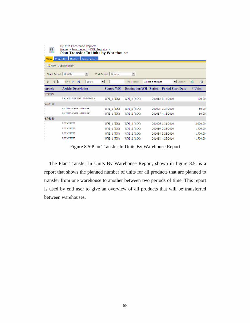
65
Figure 8.5 Plan Transfer In Units By Warehouse Report
The Plan Transfer In Units By Warehouse Report, shown in figure 8.5, is a
report that shows the planned number of units for all products that are planned to
transfer from one warehouse to another between two periods of time. This report
is used by end user to give an overview of all products that will be transferred
between warehouses.
66
9. Continuing Work
As the Demand Forecast Planner continues to be used, it will undoubtedly
require additional alterations to meet the changing needs of its end users. While
all of these changes are not yet known, one such change that is expected in the
future is the forecasting of future monetary liabilities based off data within the
Demand Forecast Planner. Currently, the system deals with inventory units that
are required to meet future sales, but gives little insight into the projected cost of
these units. The customer has expressed interest in such a change, but wants to
ensure the system is satisfactory at providing unit projections before dollars and
budgeting are associated with the system.
Another expected change is the automated creation of purchase orders. As the
system works today, it only predicts future inventory needs and does nothing to
interface with the system that actually places orders for those inventory needs.
This process is done manually by a user of the system and can be time-consuming
and prone to data entry errors. Automating this process will save time, as well as
ensure inventory needs are not overlooked or incorrectly entered.
The last anticipated enhancement is some form of automated notification about
future inventory levels. The Demand Forecast Planner today is completely driven
by an end user analyzing data for future inventory needs. A set of automated rules
and email alerts will likely be created to make using the Demand Forecast Planner
more reactive rather than proactive and ensure inventory needs are not
overlooked. This should also reduce the number of hours spent using the system,
and thus the overall expense of purchasing inventory for the company.

67
10. Conclusion
Inventory may not be the most important aspect of the direct sales industry, but
without proper inventory management a direct sales company is destined for
failure. This thesis describes the software life cycle used to design, implement and
test a tool called the Demand Forecast Planner. This tool gives precise, current
and easily accessible data on past sales, inventory and consumer trends that can be
used to manage the purchasing of inventory. The detailed insight given by the
Demand Forecast Planner also allows for a more precise estimate of future
inventory needs, and thus can be used to reduce the amount of capital committed
to working inventory. Additionally, accurate inventory management frees up
distributors to do what they do best–make sales. When distributors do not have to
worry about if the products they are selling is in stock, they can focus all efforts
on selling and thus make the direct sales business model function as designed.
The Demand Forecast Planner not only gives end users detailed information
into past sales, inventory and consumer trends, but does so in a clear, easy-to-read
manner. One of the key issues that led to the creation of the Demand Forecast
Planner was not a lack of information, but rather too much information scattered
in different locations. Properly aggregating the raw data into easily
understandable objects was one of the major goals accomplished by this tool. This
not only made displaying data in a clear and easy-to-read manner possible, but
facilitates a logical path for future enhancements.
The well-defined software engineering principals used to build the Demand
Forecast Planner not only created an application that met the needs of the
customer, but did so in a manner that was concerned with proper documentation,
future expansion and completeness of design for the system. Starting with
defining requirements and the use of software engineering principals clearly
described what the system was to do. The design phase built upon these
requirements not only to define how the system would be implemented, but how
to do so in an expansion minded and efficient way. Software engineering

68
principles were used to properly write the source code and define test cases that
would test if the requirements were implemented correctly. Lastly, these
principles were applied to the maintenance of the system to ensure enhancements
adhered to the same software engineering process used to build the system in the
first place. Without the use of software engineering principles, it is unlikely the
Demand Forecast Planner would be the successful software system it is today.
69
11. Bibliography [1] Peter Landerud, “DFP Terms-Definitions-Functionality”, HyCite
Corporation, 2008.
[2] Peter Landerud, “Functional Requirements Document – Demand
Forecast Planner”, HyCite Corporation, 2008.
[3] Peter Landerud, “OO Design – Demand Forecast Planner”, HyCite
Corporation, 2008.
[4] Peter Landerud, “Database Design – Demand Forecast Planner”, HyCite
Corporation, 2008.
[5] Peter Landerud, “Test Plan – Demand Forecast Planner”, HyCite
Corporation, 2008.
[6] IEEE Standards Board, “IEEE Standard Glossary of Software Engineering
Terminology”, IEEE Std. 610.12-1990, 1990.
[7] IEEE Standards Board, “IEEE Recommended Practice for Software
Requirements Specifications”, IEEE Std. 830-1998, 1998.
[8] IEEE Standards Board, “IEEE Recommended Practice for Software
Design Descriptions”, IEEE Std. 1016-1998, 1998.
[9] IEEE Standards Board, “IEEE Standard for Software Test
Documentation”, IEEE Std. 829-1998, 1998.

70
[10] Robert N. Charette, “Why Software Fails”, IEEE Spectrum, September
2005.
[11] Microsoft Knowledge Base, “Microsoft Consulting Services Naming
Conventions for Visual Basic”, Article ID 110264, Microsoft Corporation,
January 2003.
[12] Eric Woodruff, “Sandcastle Help File Builder”,
http://www.codeplex.com/SHFB, 2004.


