

Design and Analysis of Network Codes
Thesis by
Sidharth Jaggi
In Partial Fulfillment of the Requirements
for the Degree of
Doctor of Philosophy
California Institute of Technology
Pasadena, California
2006
(Submitted October 28th, 2005)

ii
c© 2006
Sidharth Jaggi
All Rights Reserved

iii
But it’s not who you are underneath, it’s what you do that defines you.
– Rachel Dawes

iv
To Mom, George, Michelle, and the good people at the Caltech Y.

v
Chapter 1 Acknowledgements
Pour undergraduate student in vat, ferment for five years, decant out a Ph.D. As
with any reaction, this one required many ingredients, environmental controls, and
catalysts. (Warning – do not try this at home.) Here’s a list of some of the many
people who deserve much of the credit but none of the blame.
Claude Elwood Shannon, who was there before anyone else. Michelle Effros,
who showed me the way in more ways than one. Radhika Gowaikar and Chu-hsin
Liang were there when I needed them, and how. Naveed Near-Ansari, John Lilley,
and Michael Potter protected the world from my evil hacker-genius ways, and Linda
Dozsa, Veronica Robles, and Shirley Beatty made sure the paper trail always led
to President Nixon. My labmates-in-crime, Diego German Dugatkin, Hanying Feng,
Qian Zhao, and Chaitanya Kumar Rao, educated me in the ways of graduate student
life; in particular, I thank Michael Ian James Fleming for passing on the flame bearing
the wisdom of old age, Wei-hsin Gu for accepting it, and Mayank Bakshi and Sukwon
Kim for proving that life goes on. Jeremy Christopher Thorpe, Amir Farajidana, and
Masoud Sharif, dammit, you were always right. Jehoshua (Shuki) Bruck was my fairy
godfather, and his students, in particular Yuval Cassuto, Marc Riedel, Alex Sprintson,
Anxiao Jiang, and Matthew Cook, were surrogate labmates. Peter Sanders, Sebastian
Egner, and Ludo Tolhuizen deserve thanks for patiently bearing my bumbling efforts
at being a token-bearer. Microsoft Research, Redmond, has been good to me – Philip
Chou was the perfect mentor for a green summer intern, and set me on the path
of what would eventually turn into the beast that is this document, and my mentor
the next year, Kamal Jain, was my explorer-in-crime in strange realms of research.
Abhinav Kumar and Yunnan Wu were my companions during my self-imposed exile,

vi
and Pradeep Shenoy was a willing sounding-board. Michael Langberg gently showed
me how to simultaneously be a good collaborator and friend. Daniel Jerome Katz’s
love of what he does is infectious though luckily not fatal – I highly recommend trying
to contract the disease. Tracey Ho proved, amongst many other things, that great
minds can also think like lesser ones. Muriel Medard, Ralf Koetter, and Steven Low
have been generous in many matters – most of all with their time, which they have
donated at important check-points in my academic career. Robert J. McEliece, Jr.,
Babak Hassibi, and Leonard Schulman showed how the right candidacy committee
at the right time can make a significant difference. The Braun house tower of oracles
bears special mention – Mandyam Aji Srinivas, Aamod Khandekar, and Ravi Palanki
poured down learning from on high. Sony John Akkarakaran’s presence provided
some of the simple pleasures of life. The Patils opened their home and family to a
brash young DCBA; paying such generosity of spirit forward in equal measure will be
hard.

vii
Chapter 2 Abstract
The information theoretic aspects of large networks with many terminals present sev-
eral interesting and non-intuitive phenomena. One such crucial phenomenon was first
explored in a detailed manner in the excellent work [1]. It compared two paradigms
for operating a network – one in which interior nodes were restricted to only copying
and forwarding incoming messages on outgoing links, and another in which internal
nodes were allowed to perform non-trivial arithmetic operations on information on
incoming links to generate information on outgoing links. It showed that the latter
approach could substantially improve throughput compared to the more traditional
scenario. Further work by various authors showed how to design codes (called net-
work codes) to transmit under this new paradigm and also demonstrated exciting new
properties of these codes such as distributed design, increased security, and robustness
against network failures.
In this work, we consider the low-complexity design and analysis of network codes,
with a focus on codes for multicasting information. We examine both centralized and
decentralized design of such codes, and also both randomized and deterministic design
algorithms. We compare different notions of linearity and show the interplay between
these notions in the design of linear network codes. We determine bounds on the
complexity of network codes. We also consider the problem of error-correction and
secrecy for network codes when a malicious adversary controls some subset of the
network resources.

viii
Contents
Dedication iv
1 Acknowledgements v
2 Abstract vii
List of Figures x
3 Introduction 1
3.1 Background . . . . . . . . . . . . . . . . . . . . . . . . . . . . . . . . 1
3.2 Contributions . . . . . . . . . . . . . . . . . . . . . . . . . . . . . . . 3
4 Definitions 6
4.1 Graphs . . . . . . . . . . . . . . . . . . . . . . . . . . . . . . . . . . . 6
4.2 Network Codes . . . . . . . . . . . . . . . . . . . . . . . . . . . . . . 6
4.3 Linear Network Codes . . . . . . . . . . . . . . . . . . . . . . . . . . 9
5 Design of Multicast Network Codes 11
5.1 Centralized Design . . . . . . . . . . . . . . . . . . . . . . . . . . . . 12
5.1.1 Random Design of βe . . . . . . . . . . . . . . . . . . . . . . . 17
5.1.2 Deterministic Design of βe . . . . . . . . . . . . . . . . . . . . 17
5.2 Decentralized Design . . . . . . . . . . . . . . . . . . . . . . . . . . . 20
5.2.1 Random Code Design . . . . . . . . . . . . . . . . . . . . . . . 21
5.2.2 Deterministic Code Design . . . . . . . . . . . . . . . . . . . . 25
6 Relationships between Types of Linear Network Codes 32

ix
7 Complexity 44
7.1 Coding Delay/blocklength . . . . . . . . . . . . . . . . . . . . . . . . 44
7.1.1 Algebraic Network Codes . . . . . . . . . . . . . . . . . . . . . 45
7.1.2 Convolutional Network Codes . . . . . . . . . . . . . . . . . . 47
7.2 Per-bit Computational Complexity . . . . . . . . . . . . . . . . . . . 48
8 Networks with Adversaries 54
8.1 Introduction . . . . . . . . . . . . . . . . . . . . . . . . . . . . . . . . 54
8.2 Related Work . . . . . . . . . . . . . . . . . . . . . . . . . . . . . . . 56
8.3 Unicast Model . . . . . . . . . . . . . . . . . . . . . . . . . . . . . . . 57
8.4 Multicast Model . . . . . . . . . . . . . . . . . . . . . . . . . . . . . . 61
8.5 Variations on the Theme . . . . . . . . . . . . . . . . . . . . . . . . . 67
8.6 Non-causal Adversary . . . . . . . . . . . . . . . . . . . . . . . . . . . 70
8.6.1 Unicast . . . . . . . . . . . . . . . . . . . . . . . . . . . . . . 71
8.6.2 Multicast . . . . . . . . . . . . . . . . . . . . . . . . . . . . . 73
9 Summary and Future Work 77
9.1 Summary . . . . . . . . . . . . . . . . . . . . . . . . . . . . . . . . . 77
9.2 Future Work . . . . . . . . . . . . . . . . . . . . . . . . . . . . . . . . 79
Bibliography 81

x
List of Figures
6.1 Diagrammatic representation of relationships between different notions
of linearity . . . . . . . . . . . . . . . . . . . . . . . . . . . . . . . . . 34
6.2 This figure shows a single-sender (S) single-receiver (R) network Gn,
such that both branches of the network have n edges. Sub-figures
(a), (b), and (c), respectively, show particular block, algebraic, and
convolutional network codes for Gn. . . . . . . . . . . . . . . . . . . 37
7.1 An example of a 3-layer graph . . . . . . . . . . . . . . . . . . . . . . 45

1
Chapter 3 Introduction
3.1 Background
Once in a while, a simple observation can have far-reaching consequences. Shannon’s
seminal results [59] forming the basis of information theory relied on the underlying
ideas that data storage and transmission systems could be modeled stochastically,
and that almost all codes are “good.” Yet, efficient design and implementation of
codes that achieve the rate region for these problems is not always easy; for many
problems only the existence of good codes are known, and polynomial-time construc-
tions, encoding and decoding is not known. Further, generalizing most point-to-point
communication results to general networks turns out, for many problems, to be much
harder. Much further work by many researchers led to results on networks with a
“few” nodes or with some simple structure, but for many classical information theo-
retic problems even a tight characterization of the rate-region is not known.
Against this backdrop of unknown rate regions, computational intractability in
code designs, and a lack of analytical tools to attack network information flow prob-
lems, the results of the field of network coding seem especially remarkable and excit-
ing. The work in [1] examines the class of multicast problems, i.e., information flow
problems where one source wishes to transmit all of its information over a network
to a set of prespecified sinks, each of which wishes to receive all of the information.
The classical paradigm for flow of information over a network involves intermediate
nodes being passive copiers and forwarders of information on incoming links to out-
going links. Under this restricted class of operations, even computing the rate-region
of multicast problems within a constant multiplicative factor is computationally in-

2
tractable [35].
In contrast, as stated on the network coding home-page [48], “the core notion of
network coding is to allow and encourage mixing of data at intermediate network
nodes.” The work in [1] gives a tight characterization of the rate region, such that the
simple min-cut upper bounds is matched by random codes in which each intermediate
node performs a random operation on its incoming messages to produce outgoing mes-
sages. Further, it can be shown [33] that the throughput achievable by network codes
can be arbitrarily larger than the throughput achievable by routing-only schemes.
Recently, there has been a steady trend towards ever simpler designs and imple-
mentations of network codes. Work by [45] shows that the same rate region remains
achievable even when all operations in the network are restricted to be linear over an
appropriate field, and the work of [37] shows that such codes can be designed over
appropriate finite fields and gives explicit (though exponential-time) algorithms to
design such codes. Linear codes are important for three reasons. First, as shown
by [37] and [45], restricting oneself to the class of linear codes does not reduce the
capacity region for an important class of network coding problems that includes mul-
ticasting. Second, the complexity of implementation of such codes is polynomial in
the blocklength n, which is attractive from an implementation point of view. Lastly,
prior known results in linear algebra give us guidance in designing linear network
codes with provably good performance; such guarantees are difficult to provide for a
larger class of codes.
Independent work by [57] and [30] (combined in [33]) gives the first polynomial-
time design algorithms for network codes. This sets the stage for the design of network
codes that are not only low complexity in encoding and decoding, but also in design.
Concurrent and independent work by three groups [30], [58] (unpublished), and [25]
examines the low-complexity distributed random design of network multicast codes.
This set of results is particularly interesting from a network practitioner’s point of

3
view; they indicate a means of operating networks in a decentralized manner, and
yet simultaneously attaining theoretically optimal throughputs. Such random dis-
tributed codes are provably robust against failure of network resources such as links
and edges, and their throughput degrades gracefully with successively more serious
network failures [7]. An excellent survey on random coding techniques and results
can be found in [23].
Some other applications of network coding include [11], which considers the prob-
lem of quickly disseminating information from multiple sources to all nodes in a
network, and [62], which shows how using network coding ideas in ad hoc wire-
less networks can reduce the average energy required per transmission. The work
in [34], [18] considers secrecy issues for networks and shows how using network codes
can help improve network security.
The interested reader is encouraged to visit the network coding home-page [48] to
access more references.
3.2 Contributions
The central contributions of this thesis are in the areas of low-complexity deterministic
and randomized designs of network codes for multicast problems, classification of
types of linear network codes and analysis of their complexity, and of design of network
multicast transmission protocols in the presence of a malicious hidden eavesdropping
and jamming adversary.
Chapter 5 examines the low-complexity design of network codes for multicast
problems. The first polynomial-time centralized code designs for both deterministic
and randomized code design algorithms are demonstrated; these design algorithms
make designing multicast network codes computationally tractable. A decentralized
code design is also presented, which at the cost of an asymptotically negligible error

4
probability allows for very low-complexity code design, resulting in codes that require
minimal network management, and are robust against failures of network nodes and
links. Also presented are some deterministic decentralized code designs that guarantee
the correctness of the designed code, at the cost of greater complexity in either code
design or code implementation.
In Chapter 6, we examine three different notions of linearity – algebraic, block,
and convolutional linear network codes. For some of these reductions that convert
codes designed under one notion of linearity into codes that are linear under another
notion of linearity are shown. This allows for a single code design mechanism for
all three types of linear codes, and also indicates methods for reconciling different
types of linear operations in different parts of the network. For some other notions
of linearity, it is shown that no such reductions can exist. A distinction is made
between reductions for multicast network codes and those for general network coding
problems. We also distinguish between reductions that are local, and can therefore
be implemented in a decentralized manner, and those that are global, and therefore
require a central controlling authority. These reductions show the advantages and
limitations of each kind of linear network code, depending on the particular type of
network coding problem at hand.
We analyze different notions of the complexity of implementation of network codes
in Chapter 7. One notion, the delay complexity, considers the minimal alphabet
size required for the network code to achieve optimal throughput. Upper and lower
alphabet size bounds for the case of multicast network codes are presented; these
bounds match up to a multiplicative factor of 2. It is shown that using convolutional
codes can further reduce the required field-size by a factor of two. Another notion
of complexity, the number of bit operations required for each encoding operation to
generate a single decodable bit at the sink, is also examined. In particular, we design
a class of randomized block codes we call permute-and-add codes and show that they

5
require a number of bit operations that is the lowest possible – only as many as are
required by routing-only network codes.
Lastly, we consider in Chapter 8 error-correction and secrecy for network codes
when a malicious adversary controls some network resources. The motivation behind
considering this problem is the scenario where a rogue hidden network component,
either passively or actively malicious, injects fake information into the network; since
interior nodes in a network code mix all information coming on incoming links to
generate messages on outgoing links, this is potentially catastrophic, since all the in-
formation in a network could be corrupted by a single bad node. We design codes to
transmit information in this scenario. The computationally unbounded, hidden ad-
versary knows the message to be transmitted and can observe and change information
over the part of the network he controls. The network nodes do not share resources
such as shared randomness or a private key. We demonstrate that if the adversary
controls a fraction p < 0.5 of the |E| edges, the maximal throughput equals (1−p)|E|,
otherwise it equals 0. We describe low-complexity design and implementation codes
that achieve this rate region. We then extend these results to investigate more general
multicast problems in networks with adversaries.
6
Chapter 4 Definitions
4.1 Graphs
Let V be a set of vertices and E ⊆ V × V × Z be a set of unit-capacity directed
edges, where e = (v, v′, i) ∈ E denotes the ith edge from v to v′. An edge of the form
e = (v, v, i) is called a self-loop. The tuple (V, E) defines a directed graph G.
For a node v ∈ V, let ΓO(v) denote the set of edges (v, v′, i) outgoing from v and
ΓI(v) denote the set of edges (v′′, v, i) entering v. An edge e = (v, v′, i) is said to have
tail v, denoted by v = vt(e), and head v′, denoted by v′ = vh(e).
An ordered set u1, i1, u2, i2, . . . , in−1, un is said to be a path P (u1, un) from u1
to un in G if (uj, uj+1, ij) ∈ E for all j ∈ 1, . . . , n− 1. Two paths P and P ′ are said
to be edge-disjoint if they do not share edges in common. A path P (u, v) is said to
be a cycle if u = v. A graph G is said to be acyclic if it contains no cycles.
For any S ⊆ V, a cut Cut(S) ⊆ E is the set of all edges (v, v ′, i) such that v ∈ S,
v′ ∈ V \S. The value of Cut(S), |Cut(S)| equals the size of Cut(S). A min-cut from
v to v′ Mincut(v, v′) is any Cut(S) of minimum size such that v ∈ S and v′ /∈ S. The
value of Mincut(v, v′), |Mincut(v, v′)|, equals the size of Mincut(v, v′).
4.2 Network Codes
The graph G contains pre-specified sets S of source vertices and T of sink vertices.
For each s ∈ S, R(s) ∈ Z is called the source rate at s. Time is discrete and indexed
by non-negative integers. Let X = 0, 1. At time i, each s ∈ S generates Bernoulli-
(1/2) random bits Xsi = Xs
i,jR(s)j=1 ∈ XR(s). All Xs
i are independent and identically
7
distributed.
A connection χ(s, t) is a triple (s, t, Xs,ti ) ∈ S × T × X s
i . The random variables
Xs,ti comprise the message from s to t. The rate from s to t, R(s, t) is defined as
|Xs,ti |. A network coding problem P(G) is a set χ(s, t) of connections in G.
Network coding problems of particular interest are multicast network coding prob-
lems. In such problems, there is a single s ∈ S with source rate R. For each t ∈ T ,
Xs,ti = Xi.
Each s ∈ S possesses a source encoder Xaviers. Each t ∈ T possesses a sink
decoder Yvonnet. Every other node in V possesses an internal encoder. A network
code C is defined by its source encoders, internal encoders, and decoders at receiver
nodes. Permissible arithmetic operations in C are now described.
Let alphabet size q be a design parameter for C, and let q = 2b for some positive
integer b. The alphabet 0, 1, . . . , q−1 of C is the finite field Fq. For each s ∈ S source
bits are blocked into b-dimensional vectors that are treated as elements of the finite
field Fq. In particular, (Xsib+1, . . . , X
sib+b) becomes Xs(i) ∈ Fq and (Xs,t
ib+1, . . . , Xs,tib+b)
becomes Xs,t(i) ∈ Fq.
We first consider block network codes for acyclic graphs. A design parameter for
block network codes is the blocklength n. Let Y e be the length-n vector transmitted
across edge e, defined inductively as follows.
For each s ∈ S the source encoder Xaviers comprises a collection of functions
f s,ee∈ΓO(s). For each e ∈ ΓO(s), f s,e : (Fq)nR(s) → (Fq)
n maps source vector Xs to
the vector Y e transmitted across edge e.
For each s ∈ S and each e /∈ ΓO(s) the internal encoder is a function f s,e :
(Fq)n|ΓI(vt(e))| → (Fq)
n that maps messages Y e′ on all links e′ incoming to vt(e) to the
vector Y e transmitted across edge e. In multicast networks with only one source, we
abbreviate f s,e as f e.
The channel ge for each edge e ∈ E is an identity function unless explicitly defined

8
otherwise.
For each t ∈ T , the sink decoder Yvonnet comprises a collection of functions
hs,ts∈S . For each s ∈ S, hs,t : (Fq)n|ΓI(t)| → (Fq)
nR(s,t) maps the collection Y t =
(Y e)e∈ΓI(t) of received channel outputs to a reconstruction Xs,t of message Xs,t. For
multicast network codes we denote the decoders as ht.
The error probability is defined as
P (n)e = Pr∃χ(s, t) ∈ P(G) such that Xs,t(Y t) 6= Xs,t.
The rate-vector R(P(G)) = (R(s, t))χ(s,t)∈P(G) is achievable if for any ε > 0 and n
sufficiently large there exists a blocklength-n network code C with P(n)e < ε. The
capacity-region C of the network G equals the convex hull of the achievable rates.
The network code C is said to solve with zero error the network coding prob-
lem P(G) if Xs,t = Xs,t for every χ(s, t) in P(G). The rate-vector R0(P(G)) =
(R(s, t))χ(s,t)∈P(G) is achievable without error if for n sufficiently large there exists
a blocklength-n network code C that solves P(G) with zero error. The zero error
capacity-region C0 of the network G equals the convex hull of the rates achievable
without error. For multicast network codes C and C0 are scalars.
Block network codes are not well-defined for networks with cycles. In such cases
(and some other cases to be specified later) sliding window network codes CSW are
useful. Sliding window network codes differ from block network codes in their encoders
and decoder definitions.
For each s ∈ S the source encoder Xaviers comprises a collection of functions
f s,e,SWe∈ΓO(s). For each e ∈ ΓO(s) and for each time i, f s,e,SW : (Fq)n(R(s)+|ΓO(s)|) →
Fq maps Xs(j), Y e(j)e∈ΓO(s)ij=i−n to the ith symbol Y e(i) transmitted across edge
e.
For each s ∈ S and all edges e /∈ ΓO(s) and for each time i the internal encoder is

9
a function f e,SW : (Fq)n(|ΓI(vt(e))|+|ΓO(vt(e))|) → Fq that at time i maps the n previous
symbols Y e(j)e∈ΓI(vt(e))∪ΓO(vt(e))ij=i−n on all links e′ incoming to and outgoing
from vt(e) to the ith symbol Y e(i) transmitted across edge e. For multicast network
codes, we denote the encoders as f e,SW .
For each t ∈ T , the sink decoder Yvonnet comprises a collection of functions
hs,t,SWs∈ΓO(s). For each s ∈ ΓO(s), hs,t,SW : (Fq)n(|ΓI(t)|+|ΓO(t)|) → (Fq)
R(s,t) maps
the collection Y t = Y e(j)e∈ΓI(t)∪ΓO(t)ij=i−n of n previous received channel outputs
to a reconstruction symbol Xs,t(i) of message Xs,t(i). For multicast network
codes we denote the decoders as ht,SW .
The error probability, capacity region and zero error capacity region for sliding
window network codes are defined in a manner similar to that of block network codes.
4.3 Linear Network Codes
We define three important classes of linear network codes.
An F2m-network code is a block network code such that the alphabet q = 2m, the
blocklength n = 1, each encoder f s,e and f e is of the form Σe′∈ΓI(vt(e))βe′,eY e′ and
each decoder hs,t is of the form (Σe′∈ΓI (t)βe′,eY e′)e∈ΓO(t). Here all βe′,e and Y e′ are
elements of F2m and all operations are linear over Fq. Another name for F2m network
codes is algebraic linear network codes [37].
An (F2)m-network code is a block network code such that q = 2, n = m, each
encoder f s,e and f e is of the form Σe′∈ΓI (vt(e))[βe′,e]~Y e′ and each decoder hs,t is of the
form (Σe′∈ΓI(t)[βe′,e]~Y e′)e∈ΓO(t). Here all [βe′,e] are m × m matrices over F2, ~Y e′ are
length-m vectors over F2, and all operations are linear over F2. Another name for
(F2)m network codes is block linear network codes [30].
A degree-m F2(z)-network code is a sliding window network code such that q = 2,
n = m, each internal encoder f e,SW is of the form Σe′∈ΓI (vt(e))βe′,e(z)Y e′(z), and
10
each decoder hs,t,SW is of the form (Σe′∈ΓI(t)βe′,e(z)Y e′(z))e∈ΓO(t). Here all βe′,e(z) are
rational functions in z over F2 with degree of numerator and denominator at most
m, Y e′(z) = ΣY e′(i)zi are polynomials in z over F2, and all operations are linear over
F2(z). Another name for degree-m F2(z) network codes is degree-m convolutional
linear network codes [16]. If all βe,e′(z) are polynomials of degree at most m in z,
then the network codes are said to be FIR (Finite Impulse Response) degree-m F2(z)-
network codes. Otherwise, each βe,e′(z) is a ratio of polynomials of degree at most m
in z, and such network codes are said to be IIR (Infinite Impulse Response) degree-m
F2(z)-network codes.
For all three types of linear network codes, the global coding measure for edge
e ∈ E . describes the linear transformation of the information from the sources that
traverses edge e. In particular, for algebraic network codes, if e carries the symbol
β1X(1)+· · ·+βCX(C), then the global coding vector βe equals [β1, . . . , βC ]T . For block
network codes, if e carries the length-n vector [β1]X(1)+· · ·+[βC ]X(C), then the global
coding matrix [βe] equals the matrix [[β1] . . . [βC ]]T . For convolutional network codes,
if e carries the bit-stream whose z-transform equals β1(z)X1(z) + · · · + βC(z)XC(z),
then the global coding filter βe(z) equals the vector [β1(z) . . . βC(z)]T .
We note that the above three types of linear networks codes are not the most
general possible. For instance, the case of block linear network codes with infinite
blocklength is not considered.

11
Chapter 5 Design of Multicast Network
Codes
In this chapter we consider the design of linear network multicast codes. We consider
both centralized and decentralized designs. In centralized design, a central authority
with knowledge of the entire network’s topology is in charge of designing the network
code. This leads to efficient design of network multicast codes with guarantees of
correctness. Some such codes were first considered in [37], but no polynomial-time
design algorithms were known before [33].
The centralized design paradigm assumes the existence of a network management
authority that not only has a large amount of knowledge about a possibly dynamic
network, but also is able to dictate to individual network nodes the particular coding
operations they must perform. Since centralized design is not always possible, we
also consider a decentralized code design paradigm wherein each interior node of the
network, chooses its own coding operations without knowledge of the code at other
nodes in the network. The overall effect of these decisions can be percolated down
the network using small headers, which enables the receivers to decode the messages
received on incoming links. Similar results were concurrently shown in [25].
For both the centralized and decentralized paradigms we consider both determin-
istic and randomized code designs, which result in algorithms with varying properties
in terms of design and implementation complexities.
We consider only designs for directed acyclic graphs. For networks with cycles,
extensions of the arguments presented below appear in [16], where a centralized design
is discussed, and in [27], where a distributed randomized design is proposed. The case

12
of undirected networks is examined in [46].
5.1 Centralized Design
We first present a deterministic centralized algorithm, which provides intuition about
the underlying algebraic formulation of the design problem. We begin with an infor-
mal outline, which describes the underlying principles in designing an F2m-network
code.
Our algorithm consists of two stages. In the first stage, a flow algorithm (see
for instance [2]) is run to find, for each sink t ∈ T , a flow to sink t, i.e., a set
F t = Pj(s, t)tj=1 of C edge-disjoint paths Pj(s, t) from the source s to sink t. Only
the edges in the union of these flows over all sinks are considered in the second stage
of the algorithm.
The second stage is a greedy algorithm that visits each edge in turn and designs
the linear code employed on that edge. The order for visiting the edges is chosen so
that the encoding for edge e is designed after the encodings for all edges leading to e.
The goal in designing the encoding for e is to choose a linear combination of the inputs
to node vt(e) that ensures that all sinks that lie downstream from e obtain C linearly
independent combinations of the C original source symbols X = (X(1), . . . , X(C)).
When designing a linear encoding function f e for any edge e, the algorithm maintains
a set Dt,e ⊂ E , and a C × C matrix Bt,e for each sink t. Set Dt,e, called the frontier
edge-set of t, describes the most recently processed edge e in each of the C edge-
disjoint paths in F t. The C columns of Bt,e correspond to the C edges in Dt,e,
and the column for edge e ∈ Dt,e, denoted βe, describes the linear combination of
X(1), . . . , X(C) that traverses edge e. This is the global coding vector for edge e.
That is, if e carries the symbol β1X(1)+ · · ·+βC(C), then the corresponding column
of Bt,e is βe = [β1, . . . , βC ]T . The algorithm maintains the invariant that the matrix

13
Bt,e of global coding vectors is invertible for every t and e, thereby insuring that the
copy of X(1), . . . , X(C) intended for sink t remains retrievable with every new code
choice.
The following lemma will help us prove the existence of encoders f e with the
required properties. Let k be a fixed positive integer, and for each i ∈ 1, 2, . . . , k
let Mi be an arbitrary non-singular n × n matrix over the finite field Fq. For all
i ∈ 1, 2, . . . , k, let vi be some row vector of Mi. Let L be any subspace of (Fq)n
containing the span of v1, . . . , vk. For all i ∈ 1, 2, . . . , k, let Si be the linear span
of all the row vectors of Mi except vi, i.e., Si = spanrows(Mi)\vi. Let ⊕ represent
the direct sum of two vector spaces. We are interested in the satisfiability of the
following condition
∃ vector v such that Si ⊕ v = (Fq)n ∀i ∈ 1, 2, . . . , k. (5.1)
Lemma 1 For q ≥ k, (5.1) is always satisfiable. Further, the probability that a v
chosen uniformly and at random in L satisfies (5.1) is greater than 1 − k/q.
Proof: We note that L − ∪ki=1Si equals L − ∪k
i=1(L ∩ Si), and by using a counting
argument on the set L − ∪ki=1(L ∩ Si) we shall get the required result. Let d(L) be
the dimension of the vector space L. Then the number of vectors in L equals qd(L).
For each i ∈ 1, 2, . . . , k, the dimension of the vector space (L ∩ Si) is strictly less
than d(L), since L contains at least one vector, vi, that is not contained in Si. Hence
for each i ∈ 1, 2, . . . , k the number of vectors in L∩Si equals at most qd(L)−1. Also,
each L ∩ Si contains the zero vector, and therefore the total number of vectors in
∪ki=1(L ∩ Si) is no more than k(qd(L)−1 − 1) + 1. Since k ≤ q, the probability that a
randomly chosen v ∈ L satisfies v ∈ Si for any i ∈ 1, 2, . . . , k is at most k/q. 2
Our main result for centralized design is given in Theorem 2 below. A similar al-
gorithm with asymptotically better running-time was independently presented in [57],

14
and a combined version published in [33].
Theorem 2 ([30]) For any G there exists an F2m-network code C that solves the
multicast network coding problem for any R ≤ C and m = dlog2 |T |e. The random-
ized complexity of designing C is O(|E||T |(C)3), and the deterministic complexity of
designing C is O(C|E||T |(C + |T |)2 + |E||T |4).
Proof: As shown in [1], the rate region is defined by R ≤ C. We describe a design
algorithm to produce codes at R = C.
Algorithm Inputs: The 4-tuple (G, s, T , R).
Algorithm Outputs: The encoders f e for all e ∈ E , decoders htt∈T .
Preprocessing: A low time complexity maximum flow algorithm (for instance [2]) is
run |T | times to obtain a set of edge-disjoint paths between s and each t ∈ T . We
define the network flow F T between s and T as the union of the edges in the flows
of rate C to each ti, i.e., F T = ∪t∈T F t = e ∈ E : ∃j, t such that e ∈ Pj(s, t). Our
network only uses edges in F T , rather than possibly all edges in E . The edges in
F T are numbered from 1 to |F T | in a manner consistent with the partial order on
e ∈ E (i.e., for any edges e and e′, vh(e) = vt(e′) implies e < e′). Given the encoding
functions f e at each node, one can compute the global coding vectors βe for each
e ∈ E in a consistent manner by inductively computing βe =∑
e′∈ΓI (vt(e))βe′,eY e′.
The set βe′,e : e′ ∈ ΓI(vt(e) defines the linear encoding function f e.
Also, a step-counter a that keeps track of the edge encoding function is being
designed is initialized to 1. Henceforth, m = dlog2 |T |e.
To make definitions easier, append edges e(−1), e(−2), . . . , e(−C) to the net-
work such that vh(e(−j)) = s for all j ∈ 1, 2, . . . , C. The message Y e(−j) transmit-
ted over edge e(−j) is the symbol X(j). For each j ∈ 1, 2, . . . , C, the global coding
vector βe(−j) corresponding to e(−j) is initialized as the length-C vector with 1 in
the jth position and 0 everywhere else. Thus the global coding vector matrices B t,e

15
are initialized to the identity matrices for all sinks t ∈ T .
Calculating f e’s: At each step a ∈ 1, . . . , |F T |, the frontier edge set for sink t
at step a is defined as an ordered set Dt,e(a) containing C edges with the following
properties. The jth edge in Dt,e(a) is the edge e(a′) in Pj(s, t) with the largest value
of a′ less than or equal to a. The frontier edge set matrix for sink t at step a is the
C × C matrix Bt,e(a) whose rows are, respectively, the global coding vectors βe(a) for
the edges in Dt,e(a).
Thus for each a, there are C distinct edges in each frontier edge set Dt,e(a). The
edges in each Dt,e(a) form a subset of a cut from s to t. At step a the design algorithm,
for each t ∈ T , j ∈ 1, . . . , C, checks whether the j th element of Dt,e(a) is the
immediate predecessor of e(a) in Pj(s, t). If so, this edge is replaced by e(a) to obtain
the updated frontier edge set Dt,e(a). The algorithm then calculates the encoder f e(step)
for e(a), and therefore the corresponding global coding vector βe(a). The global coding
vector matrices Bt,e(a−1)t∈T are also updated by replacing the vectors corresponding
to immediate predecessors of e(a) with βe(a). In particular, βe(a) is chosen to be a
global coding vector satisfying
∀t ∈ T , rank(Bt,e(a)) = C. (5.2)
By Lemma 1, this is always possible. In particular, set n = C and q = 2m. Let edge
e(t, a) be the edge in the frontier edge set Dt,e(a−1) that is replaced at step a by e(a),
and Mi in Lemma 1 be Bt,e(a−1). Finally, let L be the span of βe for all e ∈ ΓI(e(a)).
Then a direct application of Lemma 1 proves that an appropriate βe(a) can always
be found over a large enough field. We outline in the next two subsections two
subroutines (one randomized and the other deterministic) that compute appropriate
βe and the corresponding f e.
The step-counter a is then incremented by 1 and this procedure repeats until

16
a = |F T |. After the above procedure terminates, for each t ∈ T frontier edge set
Dt,e(|FT |) consists only of edges e such that vh(e = t. At this stage, all βes have been
determined, and to terminate the algorithm we need to find the decoders htt∈T .
Calculating ht: For each t ∈ T , ht is defined via matrix multiplication acting on a
subset of Y t. Let π(Y t) be a length-C column vector with jth component equal to Y e,
where e is the last edge on the jth path Pj(s, t) between s and t. Then X t = ht(Y t) =
(Bt,e(|FT |))−1π(Y t); that is, π(Y t) multiplied by the inverse of the last global coding
vector matrix for t. This operation is well-defined since by assumption the global
coding vector matrices are invertible. Therefore, by the definition of the global coding
vector matrices, for all t ∈ T , X t = (Bt,e(|FT |))−1π(Y t) = (Bt,e(|FT |))−1(Bt,e(|FT |))X =
X. 2
Note on field size: It is interesting to note that Lemma 1 is tight in the sense that for
any n > 1 and q it is possible to construct q +1 subspaces Si of dimension n− 1 such
that ∪q+1i=1Si = (Fq)
n. Hence for such subspaces there is no v that satisfies (5.1). One
particular example of such subspaces is the set of subspaces Sii∈0,1,...,q, where Si
consists of all the vectors v such that v(1) and v(2) (respectively the first and second
scalar elements of the length-n vector v) satisfy condition (5.3)
v(1) + iv(2) = 0 if i 6= q,
v(2) = 0 if i = q. (5.3)
It can be seen that any vector v must satisfy (5.3) for at least one value of i. However,
this is a purely linear-algebraic condition; it is possible that there are no networks
that actually require such a large field-size. Indeed, the best known lower bound
on the field size is q ≥ O√
|T | ([30],[44]), and it is conjectured that the minimum
field-size required for any multicast problem is of this order of magnitude. To obtain
an estimate better than q ≥ |T | on the minimum field-size, one needs stronger tools
17
than linear algebra; the topology of the network must be examined. One possible
topological bound is the minimum in-degree of any node in the network.
5.1.1 Random Design of βe
We present in this subsection a randomized subroutine to find an appropriate value
for βe for each e ∈ E .
Randomized subroutine: Without loss of generality, let βe for all e ∈ ΓI(vt(e(a)))
be linearly independent. We choose f e(a) uniformly and at random over all length-
|ΓI(vt(e(a)))| vectors. We test to see if the resulting βe(a) satisfies 5.1. If so, the
subroutine exits successfully; otherwise, it loops back.
By Lemma 1 the probability of failure for any choice of f e(a) is at most 1− |T |/q.
Therefore the expected number of attempts to find a single f e(a) is 1/(1−|T |/q), which
is O(1) for large enough q. For each choice of f e(a), the computational cost of checking
the invertibility of a single Dt,e(a) equals the cost of doing Gaussian elimination on a
C ×C matrix. Therefore the expected cost of checking that the chosen f e(a) satisfies
Equation 5.1 is O(C3|T |), and the expected cost of randomized design of a multicast
network code is O(C3|E||T |).
Note: If fast matrix-multiplication techniques are used, then the complexity can actu-
ally be reduced to O(Cω|E||T |), where ω is the best exponent for matrix inversion [8].
Similar reductions in time-complexity can be achieved in the following deterministic
sub-routine.
5.1.2 Deterministic Design of βe
We now present a deterministic algorithm for finding f e(a) for any edge e(a).
Deterministic subroutine: Let vi, Si, L, d(L), Si, and k be as defined in Lemma 1.
Let L be a d(L) × C matrix whose rows form a basis for L. First, all vectors are
written in the basis L. Then, for each i ∈ 1, 2, . . . , k, row operations are performed

18
on L and Si to obtain the (d(L) − 1) × d(L) matrix S ′i, whose rows form a basis for
L ∩ Si in the coordinate system given by the rows of L. The complexity of using
Gaussian elimination to perform this operation is O(C(C + |T |)2) for each S ′i, for a
total complexity of O(C|T |(C + |T |)2) for this step.
Since each S ′i represents a (d(L) − 1)-dimensional subspace of the d(L)-vector
space S, the null-space of the transform is of dimension 1. Hence there exists a
column vector si such that for any vector y′ in the span of the rows of S ′i, the dot-
product y′sTi equals 0. To obtain each such si, row operations are performed on S ′
i
until it contains the (d(L) − 1) × (d(L) − 1) identity matrix and a (d(L) − 1)-length
column vector s′i. The vector si then equals the row vector obtained by adjoining the
element 1 to −s′i, that is, si = (−s′Ti , 1). This gives us a compact representation of
each S ′i. The time-complexity of this operation is O(|T |3) for each S ′
i, for an overall
complexity of O(|T |4) for this step.
Finding a v such that v ∈ L but v /∈ Si for any i is then equivalent to finding a
length-d(L) row vector y such that the dot-products ysi satisfy
ysi 6= 0, for any i ∈ 1, 2, . . . , k. (5.4)
The result is the length-C vector v = yL. A vector y = (y1, y2, . . . , yd(L)) satisfying
(5.4) can be obtained via the greedy sub-subroutine described below, which requires
O(|T |3) steps. Therefore the overall time-complexity is bounded by the complexity
of finding S ′i and si, giving a total of O(|E||T |C(C + |T |)2 + |E||T |4).
Lastly, to obtain βe, we note that the components of the vector v correspond to
the elements βe′,ee′∈ΓI(vt(e)) of the encoder f e(a).
Greedy Sub-subroutine: Our sub-subroutine computes elements of a length-k column
vector c one at a time, such that any length-d(L) vector y satisfying ZyT = c satisfies
(5.4). We now show that this can be done greedily. This is, one can choose elements

19
of c = ciki=1 one at a time, such that the choice of any ci only depends on cjj<i,
and the resulting C and corresponding y satisfy (5.4).
Denote the k × d(L) matrix whose ith row vector is sTi by Z. The rank of this
matrix is in general less than both k and d(L); we partition it into two parts – the
first a full-rank subset of rows, and the second a set of rows linearly dependent on
the full-rank subset. Without loss of generality, let the first rank(Z) rows of Z be
linearly independent, and denote this rank(Z) × d(L) sub-matrix by ZI. Denote the
matrix consisting of the remaining rows of Z by ZD. Matrix ZD can be written as
the matrix product TZI for some (k − rank(Z)) × rank(Z) matrix T .
Our sub-subroutine greedily chooses elements of a length-rank(Z) column vector
cI = cii≤rank(Z). This choice induces the values cD = cjj>rank(Z), and also fixes
the vector y that generates c as ZyT .
Since all of the row vectors of Z are non-zero, the rank of Z is necessarily greater
than zero. In the first step of the greedy sub-subroutine, some arbitrary value c1 6= 0
is chosen. Now there are two possibilities – either rank(Z) equals 1, or it is greater
than 1. If rank(Z) equals 1, then cI is assigned the value (1), a corresponding vector
y is computed, and the sub-subroutine terminates. This choice of c works since all
rows of Z are non-zero multiples of the first row, and therefore each ci for i > 1 is also
a corresponding non-zero multiple of 1. If rank(Z) > 1, more coefficients of c need to
be calculated. We perform this computation inductively as follows. Let Ti and Ti,j
be the ith row vector and the (i, j)th element of the matrix T , respectively. Consider
all row vectors Ti of T that have non-zero elements only in the first b positions, and
denote them by the superscript b, as T bi . Also, initialize counter b to 2. We proceed
inductively in b. For each b we compute a non-zero constant, cb ∈ Fq, such that

20
(ZI)byT equals cb. To choose cb, we note that
(ZI)biy
T 6= 0 ⇔ (ZI)by 6= −(T )−1i,b (
∑b−1j=1(T )i,j(ZI)j)y
T
⇔ (ZI)by 6= −(T )−1i,b
∑b−1j=1(T )i,jcj = di,b,
(5.5)
where each di,b is a constant in Fq. Since rank(Z) > 1, the number of rows in ZD
is at most k − 2. Then k ≤ q = 2m implies that there are at most 2m − 2 different
values of di,b for a fixed value of b. Hence we can always find a non-zero value of cb
for which (ZI)byT = cb does not contradict (5.5). The counter b is incremented and
the process repeated until b = rank(Z). The entire greedy sub-subroutine requires
O(|T |3) steps.
5.2 Decentralized Design
Often, the network topology is unknown to the code designer, source, or sinks. Only
local information (such as number of immediately upstream and downstream nodes,
and capacities on incoming and outgoing links) is available at nodes. In such a situ-
ation, decentralized design of network codes would considerably reduce the overhead
required to first determine the network topology.
Decentralized design is also potentially useful in highly dynamic networks. Ideally,
network codes should be robust against minor changes in network topology, such as
a few nodes or links failing, or new internal nodes and sinks joining. A decentralized
design can lend such robustness when network changes do not drastically alter the
network’s fundamental properties, (e.g., its multicast capacity).
The multicast capacity is the one global network parameter that must be known
prior to multicast network code design; if one designs codes at a rate higher than
the multicast capacity, it is possible that the sinks will not be able to retrieve even a
single bit of information. We therefore assume that this information is known by the

21
source prior to code design. In fact, our randomized code design suggests a simple
decentralized algorithm to get a good estimate of the min-cut to any receiver.
We consider the distributed design of linear network multicast codes for directed
acyclic networks.
5.2.1 Random Code Design
We examine the use of block linear network codes. The source s is assumed to have
good bounds on the multicast capacity C and the network parameters |E| and |T |.
It then chooses a blocklength n and forwards the value of n to all downstream nodes,
which in turn do the same until every node knows the value.
At this point, every node v independently selects a random linear encoding func-
tion f e for each outgoing edge e ∈ ΓO(v). The global coding matrix for each e ∈ ΓO(v)
is then computed and percolated down the network. This enables the sinks to com-
pute the matrix inverse required to decode the messages coming in to them.
This paradigm was developed concurrently and independently by three groups [30], [58]
(unpublished), and [25] and [27] (which consider algebraic network codes designed in
this distributed randomized manner).
We examine a version of the distributed design of block linear network codes that
was presented in Theorem 3 [30]. This design was proposed in [30] as a means of
obtaining robustness against failures of network components, corruption by malicious
adversaries, security against eavesdroppers, and complexity of implementation.
We now present our code design scheme, followed by the proof of correctness.
Randomized Code Design: Each node v, for each e′ ∈ ΓI(v), e ∈ ΓO(v), chooses a
n×n coefficient matrix [βe′,e] such that every element of [βe′,e] is chosen independently
from every other, equals 1 with probability p, and is 0 otherwise. Probability p is
a design parameter of the problem and can take any value in [log(n)/n, 0.5]. The
resulting random block network code is denoted by CR(p).
22
We define network failure patterns as follows. Let EF ⊂ E be any subset of edges
that fail, thereby passing only an infinite string of 0s. If edge e fails, then node
vh(e) percolates news of this failure down the network to the receiver and treats the
input from e as the all zeroes vector in performing its linear encoding. Effectively,
this is equivalent to vh(e) ignoring the input on e. Let the multicast capacity of the
resulting network be denoted by CF . The failure of any node v can also be treated
in this framework, by assuming instead the failure of all edges in ΓO(v).
The following theorem on random matrices is crucial in proving our result.
Theorem 3 ([3, Corollary 2.4]) There exists a universal constant A such that for
any p ∈ [(log(n))/n, 0.5], any n > 1, and ε > 0, the probability that an n × n binary
matrix with entries independently chosen to be 1 with probability p and 0 otherwise
has rank less than nε is at most A2−nε.
This result shows that, with high probability, even very sparse random matrices are
close to full rank. This enables us to show that with high probability, block network
codes composed of sparse linear transformations still achieve rates close to capacity.
We prove several closely related results.
Theorem 4 1. There exists a universal constant A such that for any ε > 0 and
n > 1, the probability that the achievable zero error multicast rate using CR(p)
is at least C − (|E| + 1)ε is at least 1 − 2−nε+log |E||T |.
2. There exists a universal constant A such that for any ε > 0, n > 1, and any
failure pattern EF , the probability that the achievable zero error multicast rate
using CR(p) is at least CF − (|E| + 1)ε is at least 1 − A2−nε+log |T |+|E|.
3. There exists a universal constant A such that for any ε > 0, n > 1, and any set
of source nodes S including a prespecified source node s, the probability that the
23
achievable zero error multicast rate using CR(p) is at least C − (|E|+ 1)ε. is at
least 1 − A2−nε+log |T |+|V|.
Proof:
1. As in the centralized design, we impose a partial order on the edges in E . We
also define for each t ∈ T and each a ∈ 1, . . . , |E| a frontier edge-set Dt,e(a)
and corresponding global coding vector matrix Bt,e(a), which represents the bits
on each edge as a linear combination of the source bits.
As our inductive hypothesis, we assume that the rank of Bt,e(a) is nC − aε. We
then show that, with high probability, the rank of Bt,e(a+1) is nC − (a + 1)ε.
The linear transform f e(a), which takes Bt,e(a) to Bt,e(a+1), leaves all but C
rows of Bt,e(a) unchanged. Let e′ denote the corresponding edge in ΓI(vt(e(a))).
We use Bt,e(a)1 to denote the n(C − 1) × nC submatrix of Bt,e(a) that remains
unchanged and Bt,e(a)2 to denote the remaining n × nC submatrix of Bt,e(a).
Edge-set ΓI(e(a)) may contain both edges that are in Dt,e(a) and edges that
are not elements of Dt,e(a). Therefore to obtain the new global coding matrix
Bt,e(a+1), f e(a) replaces the submatrix Bt,e(a)2 by the submatrix
Bt,e(a+1)2 =
∑
e′∈ΓI(vt(e(a)))∩Dt,e(a)
[βe′,e(a)]Bt,e(a)2 +
∑
e′′∈ΓI(vt(e(a)))\Dt,e(a)
[βe′′,e(a)]LBt,e(a).
The matrix L captures the linear combinations in predecessor edges of e that
are not in frontier edge-set Dt,e(a). To prove the inductive step, we need to show
that the rows of Bt,e(a+1)2 are nearly linearly independent of those of B
t,e(a)1 (i.e.,
the dimension of the subspace of intersection is at most nε), and further that the
rank of Bt,e(a+1)2 is with high probability at least n(1−ε). By examining Bt,e(a+1)
in a basis composed of rows from Bt,e(a) and performing Gaussian elimination
on the rows of Bt,e(a+1), one can see that both of these conditions are satisfied

24
if and only if the n × n times submatrix of Bt,e(a+1) corresponding to e(a) has
rank n(1− ε). This submatrix, denoted B(t, e′, e(a)), equals [βe′,e(a)]+L′, where
L′ equals the appropriate sub-matrix of∑
e′′∈ΓI (vt(e(a)))\Dt,e(a) [βe′′,e(a)]LBt,e(a+1).
Suppose the rank of this matrix is less than n(1 − ε). Then there are at least
n(1 − ε) + 1 linearly independent vectors of length C, say y1, . . . , yn(1−ε)+1, for
which [βe′,e(a)]yi = L′′yi. By Theorem 3, the probability that this occurs is
less than A2nε. Since there are |T | global coding matrices to consider, the
probability of a rank-loss greater than nε for any a is at most 1 − |T |2nε by
the union bound. Therefore, the corresponding probability after |E| steps is at
most 1 − |T ||E|2nε. Assuming that the rank-loss at each step a is at most nε,
the overall rank-loss after at most |E| steps, equals at most |E|nε, leading to an
overall rank-loss |E|ε, which is asymptotically negligible in n.
2. The proof is very similar to that in the previous part of the theorem, except here
we need to take the union bound over all possible failure patterns as well. Since
there are at most 2|E| possible failure patterns, we have the required result.
3. The proof is again similar to that of the first part of the theorem. The difference
here is that the union bound also needs to be taken over all possible sets of source
terminals for G. Since this is at most the power-set of V, the union bound has
at most 2|V| terms. In each case, the multicast capacity is still at least C since
the min-cut from a set of vertices including s to a sink t is at least as large as
the min-cut from s to t.
2.
Distributed min-cut estimation: As a corollary to the above code design, we have a
simple means of coming up with an estimate of the min-cut from s to any t. The
source transmits random vectors of length |nΓO(s)|, with n distinct random vectors
on each outgoing edge from s. Each intermediate node chooses uniformly at random

25
among all linear combinations of vectors on incoming edges, producing n vectors on
each outgoing edge. Each sink estimates its corresponding min-cut by calculating the
rank of the collection of length-|nΓO(s)| vectors it receives and normalizing by n. The
result is a lower bound on the min-cut. By the above theorem, it is also within |E|ε
of the true value with probability exponentially close to 1 in n. Choosing ε such that
|E|ε < 1 implies that the estimate is the true value of the min-cut (since it must be
an integer). Further, while the above estimate may underestimate the min-cut with
exponentially small probability, as a lower bound it is always correct.
5.2.2 Deterministic Code Design
We now discuss various multicast code design algorithms that require only limited
global topological information. These algorithms guarantee codes with no errors,
rather than codes with asymptotically negligible error probabilities. This guarantee
is met without centralized design.
In our model,
1. Each node only knows information about the network that can be percolated
down to it from upstream nodes.
2. The source node has a good estimate of the mincut.
3. Each node has an identification number, u. Each identification number is as-
signed to only one node in the network. Let the maximal such number be
U .
4. Nodes have good upper bounds on |V|. This last assumption is not critical. We
also devise more complicated codes which do not require this information.
We call any code designed with just the above information a distributed network
code. This relatively small amount of global information enables distributed zero error

26
network code design. In comparison, the centralized design of multicast network codes
requires information corresponding to an entire cutset at each node.
We first prove a result for network multicast problems where the transmission rate
is 2. This case has also been examined in [4], in which code design is only somewhat
decentralized. We begin by stating some definitions and known results about binary
polynomials.
An irreducible polynomial over Fq is a polynomial with coefficients in Fq that
cannot be written as the product of polynomials of strictly smaller degree.
Lemma 5 The number of irreducible binary polynomials of degree m is O(m−12m).
Lemma 5 is a direct corollary of well-known bounds (see, for example, [40]) on the
number of irreducible polynomials of degree m.
Theorem 6 For any G with multicast capacity at least 2, and any multicast network
coding problem P(G), a degree-O(log(|V|U)) F2(z) zero error distributed network code
with rate 2 can be designed.
Proof: We first give a code design that results in encoders with higher than neces-
sary degree. After design of its encoding functions, each node percolates the global
coding filter used on an edge down that edge. The encoding functions are as follows.
Each node v receives on incoming edges ΓI(v) either one or two linearly indepen-
dent combinations of the source information vector (X1(z), X2(z)). If it receives just
one linearly independent combination, then it transmits this information unchanged
down all outgoing edges. If it receives two linearly independent combinations of
(X1(z), X2(z)), this enables it to reconstruct both X1(z) and X2(z) [16]. On the
jth outgoing link from v, it then transmits X1(z) + pju(z)X2(z), where pj
u(z) is the
jth power of the uth irreducible polynomial (according to the natural lexicographic
ordering on binary polynomials). By [40], the uth polynomial is of degree O(log(u)).
Each node is connected to each of at most |V| other nodes by at most two links (any
27
extra links can be removed since the rate of transmission is at most two). Therefore
the maximum degree of any polynomial in the global coding vectors of the network
code is O(|V| log(U)).
The previous design is distributed and requires no knowledge |V|. The code yields
a rate-2 network code by the following argument. We first show that each global
coding filter on each edge is of the form (1, qe(z)), where qe(z) is a binary polynomial
with the property that for any pair of edges e and e′, qe(z) = qe′(z) if and only if the
min-cut between s and vt(e), vt(e′) equals 1. This is true since if there are no edge-
disjoint paths from s to vt(e), vt(e′), then e and e′ cannot possibly carry linearly
independent information. Conversely, if there are two edge-disjoint paths from s to
vt(e), vt(e′), then the two edges leading out of s on each of these paths carry different
global coding filters, and, inductively at each stage, the global coding vectors must
be different. (By the definition of irreducible polynomials, for any two distinct pairs
(u, j) and (u′, j ′), pju(z) 6= pj′
u′(z).) This proves that the network code has rate 2, since
any two global coding filters (1, qe(z)) and (1, qe′(z)) must be linearly independent.
To decode, each receiver chooses two linearly independent incoming global coding
filters and inverts the corresponding transformation.
We now present a conceptually more complicated design that results in filters with
lower degrees, and in addition does not require any node to know how many nodes
exist in the network.
Cantor diagonal assignment: Arrange binary polynomials in a two-dimensional lat-
tice so that the (i, j)th element corresponds to the ((i + j − 2)(i + j − 2)/2 + j)th
binary polynomial according to the natural lexicographic ordering on binary polyno-
mials. It can be seen that this corresponds to arranging the lexicographically ordered
binary polynomials along successive diagonals in the positive quadrant of the two-
dimensional integer lattice. The idea for this enumerative scheme is borrowed from
Cantor’s celebrated theorem [5] showing the bijection between integers and rational

28
numbers.
If a node has only one linearly independent global coding filter on its incoming
edges, it forwards that on all outgoing edges. If it has two, then for the j th outgoing
edge from the node it choose the global coding filter (1, qu,j(z)), where qu,j(z) cor-
responds to the polynomial in the (u, j)th position on the lattice. This assignment
scheme still results in global coding filters that are pairwise linearly independent for
any two edges for which there exist edge-disjoint paths to the two edges. Hence
the scheme gives codes that are decodable. Also, the highest degree of any polyno-
mial in any global coding vector (and hence in any local encoder) can be seen to be
O(log(|V|U)). 2
The previous distributed design only works for multicast codes of rate 2. We now
demonstrate distributed design algorithms for general multicast rates R; the cost of
higher rate is either higher design complexity, or higher implementation complexity.
We first state definitions and a result which will be useful in our code design.
The following result demonstrates an elegant connection between the combinatorial
properties of a network and the existence of a network code.
Let C be a convolutional linear multicast code for the multicast network coding
problem P(G). For any such code, we define the following three matrices. The input
matrix A(z) is the C ×|E| matrix comprising the source encoders; the (i, j)th element
of A(z) equals the filter βe(−i),e(j)(z), where βe(−i),e(j)(z) equals zero if vt(e(j)) 6= s.
The line graph matrix F (z) is the |E| × |E| matrix comprising the internal encoders;
the (i, j)th element of F (z) equals the filter βe(i),e(j)(z), where βe(i),e(j)(z) equals zero
if vh(e(i)) 6= vt(e(j)). The output matrix B(z) is the |E| × |T |C matrix comprising
the decoders; the (i, j)th element of B(z) equals the decoder filter βe(i),t(z), where
βe(i),t(z) equals zero if vh(e(i)) 6= t for some t ∈ T .
Theorem 7 (Theorem 2 [27]) Convolutional code C solves P(G) if and only if the
29
corresponding Edmonds matrix is non-singular.
E(z) =
A(z) 0
I − F (z) B(z)
(5.6)
Theorem 8 shows a simple decentralized design of convolutional network multicast
codes; the codes employ exponentially large encoding and decoding filters.
We perform a pre-processing step to trim the network so that there are no more
than C edges between any two nodes.
Theorem 8 Let βu,i,j(z) represent the transfer coefficient from the ith incoming edge
to the jth outgoing edge at the node with identification u. Let
βu,i,j(z) = z2u((|V|−1)C)2+(|V|−1)C)i+j
.
Then the corresponding convolutional code C solves the network coding problem.
Proof: The function u((|V| − 1)C)2 + (|V| − 1)C)i + j is distinct for any two distinct
triples of (u, i, j). Therefore each βu,i,j(z) equals z exponentiated to a distinct power
of 2. The determinant of the Edmonds matrix E(z) equals the sum of powers of
z, each of which consists of the product of a single βu,i,j(z) from each row of the
Edmonds matrix. Therefore each term equals z exponentiated to a distinct integer,
and therefore the sum cannot be zero. Hence the Edmonds matrix is non-singular. By
Theorem 7, this implies that the code C solves the multicast network coding problem
P(G). 2
Note 1: In the above proof we assume that each node knows the value |V|. As in
Theorem 6, this can be replaced with a Cantor-diagonal assignment scheme, which
obviates this requirement. Under such a scheme, we only need to maintain the re-

30
quirement that each βu,i,j(z) = z2ν(u,i,j), where ν(u, i, j) is an integer-valued function
that takes distinct values for every distinct triple (u, i, j).
Note 2: Another scheme, which requires lower complexity filters (though still expo-
nential in length), was proposed in [24].
The above theorem is interesting in that it shows a conceptually simple distributed
design for a zero error multicast network code. However, it requires the use of pro-
hibitively expensive encoding and decoding operations, and is hence of only academic
interest.
We now show that there exist codes that require only polynomial complexity to
implement. We have only an existence proof, no polynomial-time construction has
been found to date. The proof is a simple extension of Theorem 16 in [37]. Once
again, we pare G so that there are at most C edges between any pair of nodes.
Theorem 9 For any P(G) there exists a distributed degree-O(|V|2C) F2(z) convolu-
tional network code that solves P(G).
Proof: The proof follows directly from the proof of Theorem 16 in [37], which proves
the existence of a single network code that achieves rate C over a sufficiently large field
for any of a family of networks, each with multicast capacity C. In our case, nodes in
general do not have knowledge of the entire network, but under the assumption that
they have an upper bound on the size of the network, can individually construct an
appropriate family of networks in which G is contained.
The family of networks we consider, J (C, |V|), consists of all subgraphs with min-
cut at least C, of the graph G(C, |V|) that has |V| and C edges between each pair of
nodes. By assumption, G is in J (C, |V|). A (loose) upper bound on |J (C, |V|)| is
the size of the power-set of the number of edges in J (C, |V|). Each of |V| nodes in G
is connected to most |V| − 1 other nodes, with at most C edges each. Therefore the
number of J (C, |V|) |V|2C. By Theorem 16 in [37], there exists a network code with

31
filter-size at most O(|V|2C) that achieves rate C for all networks in J (C, |V|), and
therefore in particular achieves rate C for G. 2

32
Chapter 6 Relationships between Types
of Linear Network Codes
To begin studying linear network codes, we must first answer the question “What is
linearity?” [39]. In this chapter we study relationships between algebraic, block, and
convolutional network codes. (We distinguish between FIR convolutional codes and
IIR convolutional codes.)
For a given network coding problem P(G), a reduction is a transformation of net-
work code C into a new network code C ′. We investigate reductions that enable us to
transform one type of linear network code (such as algebraic, block, or convolutional)
into another. Some of the proposed reductions apply only to a limited class of network
coding problems (e.g., multicasting), while others apply to general network coding
problems (multiple sources, multiple sinks). We distinguish between three types of
reductions.
Results currently in the literature deal with global reductions. A global reduction
for a class of networks implies that codes defined under one notion of linearity can
be replaced at every node by codes defined under another notion of linearity, and the
new codes have identical rate regions.
However, for practical codes on networks, distributed design and implementation
is desirable. We therefore consider local reductions. A local reduction is a design
algorithm for replacing codes of one type at every node of a network with codes of
another type, independently of the global network structure; the result must be a
code of the second type with a rate vector identical to that of the code of the first
type.

33
Input-output nonequivalent local reductions are local reductions that do not nec-
essarily preserve the input-out transfer function of every node. These reductions
are of interest because they enable distributed design for a new type of code when
distributed design is possible for the initial family of codes.
Input-output equivalent local reductions are local reductions that preserve the
input-output transfer function of every node. This class of reductions is of inter-
est since this enables different nodes in a network to employ different notions of
linearity.
We note that the existence of local input-output equivalent reductions implies the
existence of local input-output nonequivalent local reductions, which in turn implies
the existence of global reductions. In the reverse direction, a counter-example for
global reductions for a class of networks implies that local input-output nonequivalent
reductions for that class of networks do not exist, which in turn implies that input-
output equivalent reductions for that class of networks do not exist. In a similar
vein, the multicast network coding problem is a subset of the general network coding
problem, and a counter-example of a reduction for a multicast network coding problem
implies that no such reduction would exist for general network coding problems.
A summary of our and other previously known results is provided in Figure 6.1.
We summarize only the strongest known reductions or counter-examples.
Finally, we introduce the class of filter bank network codes, which subsume each
of the three previously mentioned classes of linear network codes. We show that
under the assumptions of causality, finite memory, and L-shift-invariance (invariance
of operations at nodes under shifts by an integer L) there exists a local input-output
equivalent reduction between any code linear over a finite field and a corresponding
filter bank network code.
We begin by reminding ourselves of some basic finite field arithmetic. In this
chapter we consider finite fields which are extensions over any prime p, rather than

34
C
B
M
M Multicast G General
GlobalLocal I/O Local I/O =
A Algebraic
B Block
C Convolutional
a Acyclic
Does not exist
epsilon rate loss
G
a
G
A Ma
Ma
G?
Ma
G
Ma
G
G
Ma
Figure 6.1: Diagrammatic representation of relationships between different notions oflinearity
simply extensions of the binary field. Let q = pm. Let Pm(z) be the degree-m
irreducible polynomial that is used to represent elements in the finite field Fq. That
is, all additions and multiplications over Fq are computed via corresponding additions
or multiplications of p-ary polynomials modulo Pm(z). This defines a one-to-one
onto linear mapping between the set of all elements of Fq and the set of all p-ary
polynomials of degree less than m. Each such p-ary polynomial can also be represented
by the length-m bit vector comprising of the coefficients of the polynomial. Several
of our proofs rely on the linear bijection BPm: Fq → (Fp)
m that takes an element in
the finite field Fq to its length-m bit-vector representation in (Fp)m. For example,
BPmtakes the multiplicative identity in Fa to the length-m bit vector with a 1 in the

35
mth position and zeroes everywhere else.
Reductions between Algebraic and block network
codes
General networks
For general networks, there exists an input-output equivalent local reduction from al-
gebraic network codes to block network codes. Even global reductions in the opposite
direction are impossible.
Lemma 10 For any algebraic network code CA,p,m that solves network coding problem
RG there exists an input-output equivalent local reduction to a block network code
CB,p,m.
Proof: Let ~ui, i ∈ 1, . . . , m be unit vectors in Fq. Given any βi′,i ∈ Fq, we define the
corresponding [βi′,i] so that its ith row vector equals BPm(βi′,iB
−1Pm
(~ui)). To see that
this preserves the input-output relationship at every node, consider the following. For
all i ∈ 1, . . . , m, let ui ∈ Fq equal (zi−1)mod(Pm(z)). Then the span of ui(z)mi=1,
with scalars from Fp, is exactly the set of p-ary polynomials of degree less than m.
Hence any element α ∈ Fpm, denoted as the polynomial (α(z))mod(Pm(z)), may be
written as∑m
i=1(aiui(z))mod(Pm(z)), where ai ∈ Fp for all i ∈ 1, . . . , m. Therefore,
due to the linearity of BPm, we are done. 2
Lemma 11 ([52],[44]) There exist network coding problems RG that are solved by
block network codes CB,p,m, such that there are no algebraic network codes CA,p′,m′ that
solve RG for any p′ and m′.

36
Multicast networks without cycles
While Lemma 11 proves that there does not exist a reduction from general block
network codes to algebraic network codes, this failure does not necessarily apply
for every network coding problem. We here examine the special case of multicast
networks.
By Lemma 10, there is a local input-output equivalent reduction from algebraic
network codes to block network codes for multicast networks. Further, by [37],[33],
algebraic network codes are optimal for acyclic multicast problems, which implies
that there exists a global reduction from algebraic network codes to block network
codes. (The case for networks with cycles is different and will be discussed in the
next subsection.)
Lemma 12 shows that local input-output non-equivalent reductions from algebraic
network codes to block network codes are not possible for multicast networks.
Lemma 12 For all n1 let CB,2,2(Gn) (i.e., the (F2)2-block network code for all net-
works of the form Figure 6(a)) be such that [β1] =
1 0
0 0
and [β2] =
0 0
0 1
.
Then for any finite field Fpm there exists a network GN such that there does not exist
an algebraic network code CA,p,m that is local input-output non-equivalent to CB,2,2(N).
Proof: Code CB,2,2(Gn) achieves a rate of 1 bit per coding instant. We wish to replace
each [β1] matrix on the left branch of the networks in Figure 6 with an element, say
β1, from a suitable finite field Fq. We also wish to replace each [β2] matrix on the
right branch with another element, say β2. Since the finite field Fpm is a cyclic group
of order pm under multiplication, for any β1, β2 in Fpm , βpm
1 = βpm
2 = 1. Thus, if the
network Gn in Figure 6 is such that n = N − 1, the messages from the two branches
will destructively interfere at the output, and the sink will receive 0 regardless of the
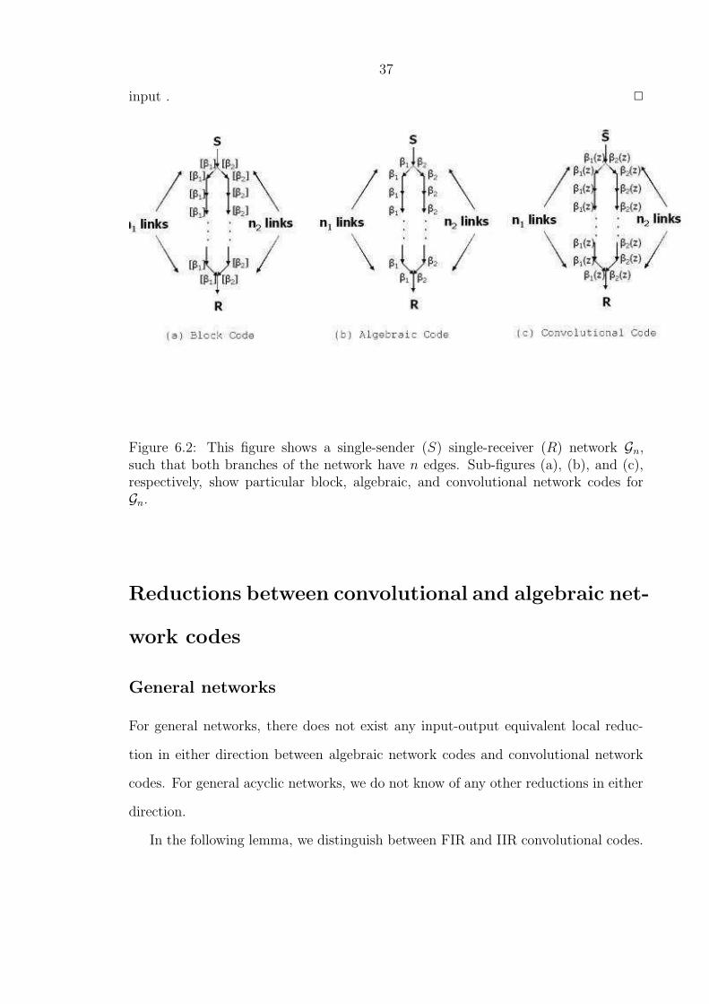
37
input . 2
Figure 6.2: This figure shows a single-sender (S) single-receiver (R) network Gn,such that both branches of the network have n edges. Sub-figures (a), (b), and (c),respectively, show particular block, algebraic, and convolutional network codes forGn.
Reductions between convolutional and algebraic net-
work codes
General networks
For general networks, there does not exist any input-output equivalent local reduc-
tion in either direction between algebraic network codes and convolutional network
codes. For general acyclic networks, we do not know of any other reductions in either
direction.
In the following lemma, we distinguish between FIR and IIR convolutional codes.

38
Lemma 13 1. For any algebraic network code CA,2,2(G) that contains a single-
input single-output node with βi′,i = (z)mod(z2 + z + 1), there does not exist a
local input-output equivalent convolutional network code CC,p,m(G) for any p, m.
2. For any convolutional network code CC,2,1(G) that contains a single-input single-
output node with βi′,i(z) = 1/(z + 1), there does not exist a local input-output
equivalent algebraic network code CA,p,m(G) for any p, m.
3. For any convolutional network code CC,2,1(G) that contains a single-input single-
output node with βi′,i(z) = z, there does not exist a local input-output equivalent
algebraic network code CA,p,m(G) for any p, m.
Proof:
1. For the algebraic code, consider the input X(n) = 1 for all n. The output due
to the incoming message equals X(n) for odd n and X(n) + X(n − 1) for even
n. No convolutional filter can mimic this behavior.
2. For the convolutional code, consider the input X(n) = 1 for n = 0 and 0
otherwise. The corresponding output has infinite support. This behavior cannot
be mimicked by algebraic codes.
3. Consider the sequence of inputs Xj(n) = δ(j) for all n, where δ(j) is the
Kronecker-δ function. On input δ(j), the output is δ(j + 1). Let us assume
that βi′,i, an element of some Fpm is input-output equivalent to z. Because the
blocklength of this βi′,i equals m, the output corresponding to input δ(j) cannot
equal δ(j + 1).
2
39
Multicast networks
Algebraic network codes that achieve the multicast capacity are not possible for some
networks with cycles. Convolutional network codes asymptotically achieve capac-
ity [1], [37] in these networks.
We show a local input-output nonequivalent reduction from algebraic convolu-
tional network codes to convolutional network codes for multicast coding problems
over acyclic graphs. This reduction, combined with the existence of algebraic codes,
simplifies the arguments presented in [16], [19]. Further, by [37],[33], algebraic net-
work codes are optimal for acyclic multicast problems. Thus there exists a global
reduction between algebraic and convolutional network codes for multicast problems
on acyclic networks.
For all n let CC,2,2(Gn) (Figure 6(c)) be such that β1(z) = 1 and β2(z) = z.
Lemma 14 shows that local reductions from algebraic network codes to convolutional
network codes are not possible for multicast networks.
Lemma 14 For any integers p, m, there exists a multicast problem P(G) such that
there is no algebraic network code CA,p,m(G) that is local input-output non-equivalent
to CC,2,2(G).
Proof: We note CC,2,2(Gn) achieves the capacity of one bit per coding cycle. The
remainder of the proof is identical to that of Lemma 12. 2
Lemma 15 For any algebraic network code CA,p,m that solves a multicast network
coding problem RG there exists an input-output nonequivalent local reduction to a
convolutional network code CC,p,m.
Proof: Given any βi′,i = (B(z))mod(Pm(z)) in CA,p,m such that B(z) is of degree
less than m, we define the corresponding βi′,i(z) in CC,p,m as B(z). We denote this
mapping by M : F2m → F2(z).

40
Let Ec′ = ec′i and Ec = eci
be any two subsets of E such that each forms a cut
of G, and Ec′ is the set of all edges that are predecessors to Ec. Let ~v(Ec′ , j) be the
|Ec′|-length vector over Fpm such that the ith entry of ~v(Ec′ , j) equals α(ec′i(j)). Let
~v(Ec, j) be the |Ec|-length vector over Fpm such that the ith entry of ~v(Ec, j) equals
α(ec′i(j)). Similarly, let ~v(z)(Ec′) be the |Ec′|-length vector over F2(z) such that ith en-
try of ~v(z)(Ec′) equals α(ec′i(z)), and let ~v(Ec) be the |Ec|-length vector over F2(z) such
that ith entry of ~v(z)(Ec) equals α(ec′i(z)). Then for all Ec′, Ec, and j, any network
code CA,p,m is defined by a linear map LEc′→Ec: (Fpm)|Ec′ | → (Fpm)|Ec| from ~v(Ec′, j)
to ~v(Ec, j). Given any such LEc′→Ec, we define L(z)Ec′→Ec
: (F2(z))|Ec′ | → (F2(z))|Ec|
as L(z)Ec′→Ec(β(z)) = M(LEc′→Ec
(M−1(β(z)))). Then L(z)Ec′→Ecdescribes the lin-
ear transformation between ~v(z)(Ec′) and ~v(z)(Ec) implemented by the convolutional
network code CC,p,m. The rank of L(z)Ec′→Ecis at least that of LEc′→Ec
(since the
(.)mod(Pm(z)) operation is linear), and therefore if CA,p,m solved a particular network
multicast problem, then so does CC,p,m. 2.
Reductions between convolutional and block net-
work codes
General networks
For general networks, there does not exist a global reduction from block network codes
to convolutional network codes [52],[44]. For some networks with cycles, block net-
work codes that achieve capacity are not possible due to feedback, but convolutional
network codes achieve capacity [1], [37]. If we weaken our requirements of reductions
to allow asymptotically negligible rate-loss, we can demonstrate the existence of an
input-output nonequivalent local reduction from convolutional network codes to block
network codes.

41
Let RG be the network coding problem referred to in [44].
Lemma 16 ([52],[44]) 1. There do not exist convolutional network codes CC,p′,m′
that solve RG .
2. There exists a block network code CB,p,m that solves RG .
Given a network coding problem RG = rst, we define the corresponding ε-loss
network coding problem RεG = rε
st so that rεst = (1− ε)rst. An ε-loss network coding
problem RεG is said to be solvable if there exists a code C such that for all s ∈ S and
t ∈ T such that rεst > 0, sink t decodes Xi(s), i ∈ 1, . . . , dm(1 − ε)e without error.
We also define the decoding delay of a convolutional network code d as the number
of coding instants from the start of encoding operations before all sinks can start
decoding their messages.
Lemma 17 Given ε > 0, network G with decoding delay d, and a convolutional
network code that solves RG, there exists a block network code that solves the RεG
network coding problem with blocklength m = d/ε.
Note: The factor d/m decreases with m, and is asymptotically equal to 0.
Proof: Each source s transmits the sequence X0(s), X1(s), . . . , Xm−d(s), 0, . . . , 0 in
the first m coding instants. Each internal node follows the time domain transfer
function of the convolutional code for the first m instants. Each sink is able to
decode the first m − d symbols of the desired source symbols, by the definition of
decoding delay. This is equivalent to m-length block network codes. The transfer
matrices at each node corresponds to the truncated time-domain transfer functions
of the convolutional network codes. 2.

42
Multicast networks
For multicast network problems, input-output equivalent local reductions cannot exist
in either direction, as the following arguments show.
Lemma 18 1. For any block network code CA,2,2(G) that contains a single-input
single-output node with [βi′,i] =
1 0
0 0
, there does not exist a local input-
output equivalent convolutional network code CC,p,m(G) for any p, m.
2. For any convolutional network code CC,2,1(G) that contains a single-input single-
output node with βi′,i(z) = 1/(z + 1), there does not exist a local input-output
equivalent block network code CB,p,m(G) for any p, m.
3. For any convolutional network code CC,2,1(G) that contains a single-input single-
output node with βi′,i(z) = z, there does not exist a local input-output equivalent
algebraic network code CB,p,m(G) for any p, m.
Proof:
1. For the block code, consider the input M(ei′(n)) = 1 for all n. The output on
edge i due to the incoming message equals M(ei′(n)) for odd n, and 0 for even
n. No convolutional filter can mimic this behavior.
The proofs of 2 and 3 are identical to that in Lemma 13
2
General Formulation for Linear Network Codes
In this section we give a general formulation for linear network codes under reasonable
additional restrictions. Let us consider linear systems that are causal, have finite

43
memory, and are L-shift invariant, i.e., operations at every node are periodic with
period L.
This restricts the set of permissible encoding operations at intermediate nodes to
be of the form
y(iL + j) =m
∑
k=1
cjky(iL + j − k) +m
∑
k=0
djkx(iL + j − k), j ∈ 0, . . . , L − 1.
The above formulation of network codes leads naturally to a state-space formula-
tion for describing encoding operations at a node, and therefore for the entire network.
These sets of operations can be implemented by filter-banks.

44
Chapter 7 Complexity
Discussions of computational complexity in previous chapters focus primarily on the
time-complexity of design. For networks that are not changing rapidly, implemen-
tation complexity may be more important. In this chapter we investigate delay and
numbers of basic arithmetic operations required as measures of implementation com-
plexity.
Other measures of complexity examined by other authors include bounds on the
number of nodes that need to perform non-trivial network coding operations. The
work in [42] finds upper and lower bounds on this number and shows that finding
the minimal number of nodes that need to perform coding is an intractable problem.
An alternative approach assigns costs to various network resources (such as links or
nodes) and designs minimal cost network codes according to these metrics [47].
7.1 Coding Delay/blocklength
We give a unified definition of coding delay based on the effective blocklength N of
the code. For an F2m-algebraic network code, an (F2)m-block network code, and a
degree-m F2(z)-convolutional network code (whether FIR or IIR), we define N as m.
In this section we do not consider hybrid network codes, which are mixtures of the
three previously defined types of networks codes. However, the results we state can in
most cases be generalized to such codes. We also restrict our attention to multicast
networks; for the general network coding problems even the rate region is not known
in general.

45
U Ts
Figure 7.1: An example of a 3-layer graph
7.1.1 Algebraic Network Codes
The upper bound on the effective blocklength of network codes described in Corol-
lary 19 follows from our deterministic code design algorithm from Chapter 5.
Corollary 19 For any directed acyclic graph G and multicast network coding problem
P(G), there exists a block network code C with effective blocklength N = dlog (|T |)e.
The smallest effective blocklength N required for general multicast network coding
problems is a quantity of interest. We exhibit a family of networks (presented in [30])
that require N of at least d(log(|T |))/2e + O(1). The result is upper and lower
bounds that match up to a multiplicative constant. Similar results were independently
obtained in [44] and [17]. In addition, in [44] the same lower bound is extended to
general block codes (including non-linear codes) and it is also shown that computing
the smallest alphabet size required to solve a particular network coding is NP-hard.
We first define the following family of three-layer graphs: Ga,C = (V, E) with
vertices V = s ∪ U ∪ T where U = 1, . . . , a, T = tW | W ⊆ U, |W | = C, and
edges E = (s, u) | u ∈ U ∪ (u, tW ) | tW ∈ T , u ∈ W. The source s constitutes the
first layer, the a nodes in U constitute the second layer, and the(
a
C
)
nodes described
by T constitute the third. Each node in T is connected by unit capacity links to a
distinct C-element subset W of U . Figs. 7.1 shows G6,3 as an example.

46
In passing, we note that this family of graphs is extremely useful in proving
performance and complexity bounds of various kinds for network coding problems.
This family of graphs is used in [33] to prove that the ratio between the achievable
multicast rates with and without network coding can be arbitrarily large and in [6] to
show that if one only cares about average throughput rather than multicasting, then
the ratio is bounded. This is also the family of graphs used in [44] to prove lower
bounds on the effective blocklength of any block codes. We prove this lower bound for
block linear codes in Theorem 20 below. We show in the next section (Theorem 22)
that for sliding window codes, this bound does not hold, but a weaker version does.
Theorem 20 Any algebraic network code that solves Ga,2 and achieves the min-cut
capacity requires an effective blocklength N = dlog(a − 1)e = d(log(|T |))/2e + O(1).
Proof: The symbol that any node u ∈ U receives is of the form β1X(1)+β2X(2), which
corresponds to a global coding vector of the form (β1, β2). If any two nodes u, u′ in U
receive symbols with global coding vectors that are linearly dependent, then the sink
t that is connected to u and u′ will be unable to decode successfully. Therefore all of
the global coding vectors corresponding to different nodes u must be pairwise linearly
independent. For any Fq, there are at most q + 1 vectors of length 2 such that any
two vectors are pairwise linearly independent. More precisely, any vector in (Fq)2 is a
multiple of one of the following q +1 vectors (1, 0), (1, 1), (1, 2), . . . , (1, q−1), (0, 1);
these vectors are pairwise linearly independent. 2
A very similar argument can be used to prove that a lower bound on the effective
blocklength N for block linear codes is also d(log(|T |))/2e + O(1). This is not the
case for convolutional network codes.
47
7.1.2 Convolutional Network Codes
Convolutional network codes can require as little as half the effective blocklength of
block or algebraic network codes, or even non-linear block codes, as is shown by the
following theorem.
We first state a lemma by Morrison [55].
Lemma 21 ([55, Section 3]) The number of pairs of coprime polynomials of degree
at most m over a finite field of size q equals q2m+2 − q2m+1 + q − 1.
The above lemma allows us to construct convolutional codes for Ga,2 with half the
effective blocklength required by block codes.
Theorem 22 ([31, Corollary 11]) There exists a convolutional network code that
solves Ga,2 and achieves the min-cut capacity and requires an effective blocklength
N = d(log(|T |))/4e + O(1).
Proof: The number of length-2 vectors of degree-m polynomials over F2, such that
any two are linearly independent, is at least 22m+1 + 1. This is because any two
vectors (β1(z), β2(z)) and (β ′1(z), β ′
2(z)) satisfying βi(z) 6= 0 and β ′i(z) 6= 0 for all i in
1, 2 are linearly independent if and only if β1(z)/β2(z) 6= β ′1(z)/β ′
2(z). The number
of distinct values that β1(z)/β2(z) can take is exactly twice the number of pairs of
coprime polynomials. Calculating the value in Lemma 21 for q = 2 and adding two
(for the vectors (1, 0) and (0, 1) gives the required result. 2
The above theorem implicitly assumes that FIR convolutional codes are used. We
conjecture that if IIR convolutional codes are used, then a reduction in N by another
factor of 2 is possible.

48
7.2 Per-bit Computational Complexity
In this section we bound the number of encoder arithmetic operations required per bit
transmitted from s to any t. In the case of the algebraic linear network codes already
designed, each Y (e) is generated by taking linear combinations of up to |T | elements
over a field Fq with at least |T | elements. Thus the message on any incoming edge
to some node v undergoes log(|T |) bit operations to produce a bit on an outgoing
edge. To compare, for replicate-and-forward strategies, only a single bit operation is
required per bit on outgoing edges. For networks with large values of C or |T |, we
may wish to reduce the encoding computational complexity.
For appropriate choice of code parameters (i.e., n = O(log(|E||T |)) and p =
(log(n))/n), the randomized code design algorithm presented in Theorem 4 results in
codes that at any node require O(log log(|E||T |)) bit operations per bit transmitted,
reducing the bit coding complexity exponentially at the cost of a negligibly small loss
of achievable rate. We here show that for a different random choice of block network
codes that we call permute-and-add codes, where each [βe′,e] is chosen to be a n × n
permutation matrix, even lower complexity is possible. This work also appears in [29].
Permutation matrices have the property that each row in any [βe′,e] has exactly 1
non-zero element. We design the permute-and-add network code Cπ as follows. Let
σU,n,R be the uniform distribution on the set of all n × nR binary matrices. For all
e ∈ E such that vt(e) = s, we choose each source encoder f e i.i.d. from σU,n,R. (Hence
our choice of source encoders actually results in dense matrices rather than sparse
ones. We conjecture that appropriately choosing sparse matrices would also result in
network codes with the desired properties, but our current proof techniques do not
suffice to prove this). Let σπ,n be the uniform distribution on the set of all n × n
permutation matrices. We choose each internal encoder f e′,e i.i.d. from σπ,n.
The transfer function from s to each t is then computed inductively (as in [25]) as

49
the linear map represented by the matrix [βt] = [[βe]Te∈ΓI(t)]T whose row vectors are
all the row vectors of all the global coding matrices for all edges e incoming to sink
t. Let rt be the rank of [βt]. Suppose rt = nR. In this case the matrix [βt] has full
column rank, and [βt]−1, any pseudo-inverse of [βt], can be used as the decoder at
sink t.
The following lemma about random permutation matrices is useful in proving our
result.
Lemma 23 Let [L] be an arbitrary n × n matrix and [β] be chosen uniformly at
random from the set of all n×n permutation matrices. For any ε > 0, the probability
that the rank of [β] + [L] is less than n(1 − ε) is at most 2−nε+log(n).
Proof: For a fixed length-n vector V , the probability that V is in the null-space of
[L] + [β] is
Pr[[β]][([L] + [β])V = 0]
= Pr[[β]][V ′ = [β]V ]
≤1
(
n
wH(V )
) ,
where V ′ represents [L]V , and wH(V ) denotes the Hamming weight of the vector V .
Here [β] acts as a random permutation on the locations of the non-zero elements of
V . Thus if V and V ′ have different weights, then Pr[[β]][V ′ = [β]V ] = 0. If V and V ′
have the same weight, then V ′ 6= [β]V unless the random permutation maps the set
of non-zero locations of V to the non-zero locations of V ′. Now let V be a random
binary vector uniformly distributed on the set of all length-n binary vectors. Then

50
the probability over V and [β] that V is in the null-space of [L] + [β] is bounded as
Pr[[β], V ]][([L] + [β])V = 0]
≤1
2n
∑
V
1(
n
wH(V )
)
=1
2n
n∑
wH(V )=0
(
n
wH(V )
)
1(
n
wH(V )
)
=n + 1
2n,
As both the permutation matrix [β] and the vector V are drawn uniformly from their
corresponding domains (of size n! and 2n respectively), the number of (V, [β]) pairs
that give V ′ = [β]V is bounded from above by
n!2n n + 1
2n= (n + 1)!
If we want to bound from above the probability, over random permutations, that the
number of vectors V in the null-space of the transformation is greater than or equal
to 2nε we can assume that in the worst case each of (n+1)!2nε permutations results in
a null-space of [L] of size 2nε. Thus the probability that the transformation has a
null-space of dimension at least nε is at most n+12nε = 2−nε, where ε′ = ε − log(n+1)
n. 2
Let εn, a parameter in the design of Cπ, be any function of n such that limn→∞ εn = 0.
Define ε′n = εn − log(n+1)n
and require limn→∞ nε′n = ∞. We now state and prove our
main result on permute-and-add network codes.
Theorem 24 For any εn > 0, with probability greater than 1 − 2−nε′n+log(|E|(||T ||+1)),
network code Cπ achieves rate R = C − (|E|+ 1)εn.
Proof: We first present a high-level outline of the proof. We need to show that with
high probability the transfer function is invertible at each sink. To prove this, using
the directed acyclic nature of G we first define a partial order on specific cutsets of G.

51
We then show that with high probability the rank of the linear transformation between
any two successive cut-sets is nearly full, i.e., almost all the information carried by
edges in one cut-set is retrievable from edges in the successive cut-set. We use the
union bound to bound by a function exponentially decaying in n the probability that
even a single linear map between successive cut-sets results in a rank-loss which is
not asymptotically negligible. We then note the composition of linear maps of almost
full-rank results in a linear map of almost full rank. Therefore the transfer-function
to each receiver is, with high probability, almost full-rank. Lastly, we show that a
random encoding function will not intersect the null-space of the transfer function to
any receiver. We next formalize these concepts. First, we initialize a step-counter a
to 1. Counter a keeps track of the stage of our inductive proof-checking algorithm.
For each step a and sink t, let Dt,a be an ordered set of C edges defining a frontier
edge set for t, and [Bt,a] be an nR × nR frontier edge-set matrix composed of the
global coding matrices [βa] for the edges in Dt,a.
Our proof-checking procedure calculates, for each t ∈ T , and each count a, the
probability of the event Et,a that the linear transformation between [Bt,1] and [Bt,a]
is of rank at least n(R − aεn)
A lower bound for Pr[][Et,a] can be obtained as follows. By the inductive hypoth-
esis, with probability 1−2−nε′n+log(|a|||T ||) the linear transformation between [Bt,1] and
[Bt,a] is of rank at least n(R− aεn). Let [Bt,a] be any matrix consisting of a subset of
rows of [Bt,a] which forms a basis for [Bt,a]. Matrix [Bt,a] is partitioned into [Bt,a
e(a)],
which corresponds to the n′ ≤ n rows of [Bt,a] that carry coding vectors of edge e(a)
and [Bt,a
D\e(a)], which corresponds to the rows that carry coding vectors for the rest of
Dt,a. Let [Bt,a] be any basis for the null-space of the linear transformation between
[Bt,1] and [Bt,a], which by the rank-nullity theorem and the inductive hypothesis is of
rank at most aεn with high probability. For the inductive step we consider the linear
transform (in the basis composed of rows of [Bt,a] and [Bt,a]) between the matrix

52
[[Bt,a]T [Bt,a]T ]T and [Bt,a+1]. We denote this linear transform by the matrix [Lt,a].
(The reason we must include [Bt,a] in the transformation is because the global coding
matrix corresponding to e(a + 1) may be linearly dependent on information carried
on edges e /∈ Dt,a.)
First, note that [Lt,a] can be represented by a nR × nR matrix. Our goal will be
to bound from below the rank of [Lt,a]. While the vectors of [Bt,a+1] may be linearly
dependent on vectors from [Bt,a], such dependencies can only increase the rank of
[Lt,a]. We therefore assume that no such linear dependencies exist. In other words
we restrict ourselves to [Lt,a], the square sub-matrix of [Lt,a] acting on [Bt,a]. Since
Dt,a and Dt,a+1 differ in only one edge (e(a) is replaced with e(a + 1)), rearranging
rows and columns gives an alternative expression for [Lt,a] given by
[Lt,a] =
I 0[
Lt,a1
] [
Lt,a2
]
+[
βe(a),e(a+1)]
.
The top blocks of [Lt,a] (the identity and the zero matrices) represent the linear
transformation of the vectors of Dt,a \ e(a) (which, by the definition of the inductive
step, are unchanged). The bottom blocks represent the linear dependencies between
[Bt,a] and the information carried on e(a + 1). Here [βe(a),e(a+1)] refers to the part
of [βe(a),e(a+1)] corresponding to which basis vectors exist in [Bt,a
e(a)]. It is therefore a
minor of the random permutation matrix [βe(a),e(a+1)] such that it is itself a random
permutation matrix. The matrix [Lt,a1 ] corresponds to the linear combinations of
global coding matrices from edges other than e(a) that contribute to the global coding
matrix on e(a + 1).
We need to show that with high probability (at least 1− 2−nε′n) the nullity of this
matrix [Lt,a] is small (at most nεn). But difference in the rank of the transformation
between [Bt,1] and [Bt,a] and that of the transformation between [Bt,1] and [Bt,a+1] is
at most the nullity of [Lt,a], which in turn is at most the nullity of [Lt,a]. Therefore,
53
by taking the union bound of the probability of a rank-loss greater than nεn over all
|T | receivers and |E| edges, we are done proving the inductive hypothesis.
We now analyze the rank of [Lt,a]. Since all but the last at most n rows of
[Lt,a] correspond to an identity matrix appended with an all-zero matrix, Gaussian
elimination results in a matrix of the form
I 0
0 [Lt,a2 ] + [βe(a),e(a+1)]
.
Therefore the rank of [Lt,a] depends crucially on the rank of [Lt,a2 ] + [βe(a),e(a+1)].
We denote the dimension of [Lt,a2 ] + [βe(a),e(a+1)] by n. By Lemma 23, the rank of
[Lt,a2 ] + [βe(a),e(a+1)] is n with probability at least 1 − 2−nε′n, where ε′n = εn − log(n+1)
n.
The above shows that the overall linear transform to any receiver is, with high
probability, close to full rank. To complete the proof we need only show that with
high probability the span of the vectors generated by the source encoder does not
intersect with the null-space of [Lt,|FT |] for any t ∈ T . The probability of such an
intersection is equals the probability that a vector space of dimension n(C−(|E|+1)εn)
(the space spanned by the source encoder’s vectors) chosen uniformly and at random
from a space of dimension n intersects a fixed vector space of dimension n|E|εn (the
null-space of Lt,|FT |). It can be computed that the probability that this event does
not occur is given by Πn(C−|E|εn)i=nεn
(1 − 2−i), which can be bounded from below by
1− n(C − (|E|+ 1)εn)2−nεn. Using the union bound over all t ∈ T gives the required
error probability. 2
Note: The above provides a proof that random distributed design of permute-
and-add network codes works with high probability. If a small amount of feedback is
permitted from each t to s, then each t can tell s the matrix [β t], and the expected
number of code-design attempts required to guarantee that the permute-and-add code
works is at most 2.

54
Chapter 8 Networks with Adversaries
8.1 Introduction
Consider the following point-to-point adversarial channel coding problem. The net-
work G consists of |E| parallel, directed, binary-input, binary-output edges E =
e(1), e(2), . . . , e(|E|) between the source s with encoder Xavier and the sink t with
decoder Yvonne. Encoder Xavier wishes to describe the source’s information across
the network. Xavier also has access to a fair coin, which he can use to generate as
many bits as he wants. Xavier and Yvonne share no private key or common random-
ness. Xavier wishes to transmit all of the information generated by s to Yvonne, who
wishes to decode the received message with asymptotically negligible error probabil-
ity. Xavier and Yvonne agree on low-complexity encoding and decoding schemes in
advance. The encoding and decoding schemes are also known to the computation-
ally unbounded adversary Zorba. The adversary Zorba knows the message generated
by s but not the outcomes of Xavier’s coin flips. Zorba can also see and control
the transmissions on Z ⊆ E , where Z has size M ; Zorba cannot observe or change
transmissions on E \ Z. Zorba wishes to minimize the rate R at which Yvonne can
reconstruct the information from s with asymptotically negligible error probability.
We first consider the case where Zorba’s interference patterns on the links he controls
can be based only on the knowledge he already possesses (code design, source mes-
sage, and causal knowledge of symbols transmitted on links he controls). We then
show, using more complex arguments, that the rate region is identical even if Zorba
has non-causal knowledge of the information transmitted on links he controls.
Previous work [28] exhibits a low-complexity algorithm for each sink to detect an

55
adversarial attack with high probability as long as there is at least one packet in the
network whose contents the adversary cannot infer.
We obtain an intriguing two-part rate region for the corresponding error-correction
problem. We construct low-complexity block codes, that asymptotically achieve the
capacity CAdv(M, |E|) = (|E| − M)1(M/|E| < 0.5) of this channel model. (The
indicator function 1(·) is one when its argument is true and zero otherwise.) Viewing
the ratio M/|E| as the noise parameter of this adversarial channel, the capacity of
the channel for the regime M/|E| < 0.5 equals |E|(1 − M/|E|). That is, it equals
the capacity of |E| parallel binary erasure channels (BECs) with erasure probability
M/|E|. This result is striking since the location of all erasures is explicitly known
to the decoder of an erasure channel whereas Z is unknown to Yvonne. Indeed, our
code construction relies on BEC channel codes. The construction also employs parity
information, which enables Yvonne to estimate, with high reliability, the set J z ⊆ Z
of links that Zorba corrupts. Yvonne decodes the messages on E \ J z. Conversely,
we show that no matter which code Xavier uses, if he transmits at a rate higher
than CAdv(M, |E|), then there exists a strategy by which Zorba can force Yvonne’s
probability of decoding error to be bounded away from 0.
Section 8.3 presents our results for the case where the network consists of parallel
edges. These set the stage for the more interesting multicast model of Section 8.4.
Non-trivial coding must be performed at internal nodes in order to achieve the mul-
ticast capacity [1]. This makes error-correction harder than in the parallel link case,
since in principle the information injected into the network by an adversary controlling
even a single link can contaminate all of the information reaching any sink.
Section 8.5 treats generalizations. These include allowing small amounts of feed-
back, which increases the rate region to (|E| − M), and knowledge at the sinks of
the adversary’s location, which enlarges the rate region to (|E| − M). In contrast,
knowledge by the source of the adversary’s location leaves the region unchanged.

56
We also show a separation between channel and network coding for this problem.
That is, if the links in the network in addition to possible adversarial interference
also suffer corruption by random noise, then overlaying network coding to combat
the adversary’s actions on top of link-by-link channel coding achieves the optimal
performance. We also provide an algorithm for detecting which edges need to be
removed from the network so as to eliminate the contamination from the information
being injected by adversaries. We then consider the case where the adversary does
not know the message at the source, showing that the maximal rate at which secret
information can be embedded in an information-theoretically secure manner into the
message being transmitted equals (1−2p)1(M/|E| < 0.5). Finally, Section 8.6 details
algorithms for a scenario where Zorba possesses non-causal information on the links
that he controls, treating both the unicast and multicast cases.
8.2 Related Work
In the class of noisy channels, where communication is limited by the presence of
random noise. Shannon’s seminal paper [59] considers the problem of reliable com-
munication over a memoryless noisy channel. Two standard noisy channel models
are the Binary Symmetric Channel (transmitted bits are flipped with probability p)
with capacity CBSC = 1 − H(p), and the Binary Erasure Channel (transmitted bits
are erased with probability p) with capacity CBEC = 1 − p. The block-interference
model presented in [51] considers a type of channel with memory. There are N par-
allel binary-input binary-output edges between the source and the sink. For each
coding interval of length n, a fraction p of these N edges are BSCs whose cross-over
probability equals 1/2, and the remaining (1 − p)N are noiseless. If the sink has
state information about the channels telling him which are noiseless and which are
not, or if n is large, the authors show that the capacity of this channel approaches

57
NCBEC(p). If state information is not known to the sink and n is small (≈ 1), the
capacity is close to NCBSC(p).
In the class of adversarial channels communication is limited by the presence
of a malicious adversary. For instance, [22] presents results on a single binary-input,
binary-output channel on which an adversary can observe the full blocklength-n chan-
nel input and change at most a fraction p of these bits. The sink is required to recon-
struct the input with asymptotically negligible error probability. While the capacity
of such channels is not known, the best known non-trivial upper bound is everywhere
less than CBSC(p) [50]. When the source and sink share a length-O(log(n)) private
key for use in a blocklength-n transmission, the channel capacity is 1 − H(p) [41].
Similar results follow when the sender and receiver share randomness instead of a
private key [10]. The work of [12] and [54] gives explicit constructions of codes with
rates approaching CBSC(p) when the computational capabilities of the adversaries are
limited. An excellent survey of results for channels with uncertainty can be found
in [43]. Results on Verifiable Secret Sharing with an honest dealer ([9],[56]) can be
used to prove some results on the secret capacities of the adversarial channel model
we consider.
8.3 Unicast Model
We start with results for the parallel-edge unicast model.
The codes we use are not linear; however, they have design, encoding, and decoding
complexity that is polynomial in all the network problem parameters.
We block both source bits and Xavier’s random coin flips into m-dimensional
vectors that we treat as elements of the finite field Fq, where q = 2m. The length-
nR source input vector is X = (X(1), X(2), . . . , X(n))T , where each X(i) vector
comprises R elements of Fq. Thus X(1), X(2), . . . , X(n) represents the R source bits

58
from the first mn units of time. The m-vector of random coin outcomes is ρ ∈ Fq.
A code against adversarial attack C is defined by its encoder f ee∈E and decoder h.
For each e ∈ E , f e : (Fq)nR ×Fq → (Fq)
n maps a source vector X and random symbol
ρ to the length-n vector Y e = (Y e(i))ni=1 = f e(X, ρ) transmitted across edge e. We
use Y = f(X, ρ) = (f e(X, ρ))e∈E to denote the full channel input and Y = (Y e)e∈E to
describe the full channel output. In particular, we use the length-|E| vectors Y (i) and
Y (i) to denote the channel input and output at time i. A decoder h : (Fq)n|E| → (Fq)
nR
maps the collection Y of received channel outputs to a reconstruction X = h(Y ) of
source message X.
Xavier and Yvonne together choose a code C = ((f e)e∈E , h). This code choice
is fixed and known to Zorba, who also has full knowledge of the source message X
to be transmitted. Zorba uses this information to choose the jamming function g
used to corrupt the channel input Y to give channel output Y . In designing his
jamming function, Zorba first chooses a set Z of edges to control. The size of Z
cannot exceed M , the jamming dimension. For each e ∈ E \ Z, Y e = Y e. For
each e ∈ Z, Zorba uses jamming functions ge,i : (Fq)nR × (Fq)
iM → (Fq) to produce
Y e = ge(X, (Y e)e∈Z) = (ge,i(X, (Y e(j))e∈Z,j∈1,2,...,i))i∈1,2,...,n; thus the corrupted
information on any edge e ∈ Z can rely on both the source message X and causally
on the channel inputs Y e on all edges e ∈ Z. For notational simplicity we henceforth
write Y = g(X, Y ) to denote the full collection of channel outputs.
The error probability is defined as P(n)e = Pr[h(g(X, (Y e)e∈Z))] 6= X). Rate R
is achievable for the channel g for jamming dimension M if for any ε > 0 and n
sufficiently large there exists a blocklength-n code C with P(n)e < ε for every jam-
ming function g in the family of jamming functions described above. The capacity
CAdv(M, |E|) equals the maximal achievable rate over all g.
We now state and prove our main result for unicast channels.

59
Theorem 25
CAdv(M, |E|) = (|E| − M)1(M/|E| < 0.5)
Further, for any n and any m = ω(log(n|E|)) there exist blocklength-n codes with
R = (1 − (|E| + 1)/n)CAdv(M, |E|), P(n)e < n|E|2−m, and complexity of design and
encoding and decoding implementation equal to O((nm|E|)2).
Proof: Upper Bounds: The bound R ≤ |E| − M is immediate since Zorba can set
Y e = 0n for all e ∈ Z, thereby giving rate zero on all edges controlled by Zorba.
If M ≥ |E|/2, R = 0 since Zorba can use the following strategy to make decoding
with P(n)e < 1/2 impossible. Zorba selects an arbitrary jamming subset J z of size
|E| − M of Z. Then, for arbitrary X ′ 6= X and ρ′, Zorba sets Y e = f e(X ′, ρ′) for
each e ∈ J z and Y e = 0n for e ∈ Z \ J z. Yvonne does not know Z and is therefore
unable to decide which of X and X ′ to decode to, leading to an error probability of
at least 1/2.
Lower Bound: We first sketch the achievability argument and then give a precise
code construction. Assume M/|E| < 1/2 and R = |E| − M . In the first n − |E| − 1
symbols on each e ∈ E , Xavier transmits X using an erasure code. Xavier uses the
remaining |E| + 1 symbols to send a marker containing ρ and D = (De)e∈E . The
vector D is a hash of the vectors (Y (i))n−|E|−1i=1 with ρ. Yvonne decodes by looking for
consistency among the received channel outputs. Since Zorba controls fewer than half
of the edges, Yvonne can determine (ρ, D) by majority rule. She then recomputes the
hash using ρ and the received transmissions. Since Zorba does not know ρ a priori,
any changes he makes on (Y e)e∈Z will, with high probability, be inconsistent with
the hash values. This enables Yvonne to determine which edges have been corrupted.
She then uses Y e from e /∈ J z to reconstruct X, via the erasure code.
We now describe our coding scheme in detail. For any n and m = ω(log(n|E|)),

60
fix R = b(1 − (|E| + 1)/n)(|E| − M)c and design the functions f e using the following
procedure.
Let L be any (n−|E|−1)|E|×nR Vandermonde matrix over Fq (such a matrix exists
since q = 2m and m = ω(log(n|E|)) [21]). For the ith edge e(i) ∈ E, the matrix Le(i),
known a priori to Xavier, Yvonne, and Zorba, is defined to be the (n− |E|− 1)× nR
matrix consisting of row [(n − |E| − 1)(i − 1) + 1] through [(n − |E| − 1)i] of L. For
all e ∈ E we define T e, U , and D as
T e = (LeX)T ,
U = (1, ρ, . . . , ρn−|E|−1) and
D = U [T e(1), T e(2), . . . , T e(|E|)]
and set Y e = (T e, D, ρ). Thus for each e ∈ E , the first n − |E| − 1 symbols in Y e
are the erasure-coded message symbols, the next |E| symbols are the hash function
output, and the last symbol is the hash-function’s key ρ.
Yvonne’s decoding scheme h is as follows. Let Y e =(
T e, D, ρ)
denote the channel
output on e ∈ E . As described above, Yvonne first determines the correct value of
the marker (D, ρ) by choosing the value that appears on the majority of the links.
She then checks, for the ith edge e(i) ∈ E , whether or not the ith symbol of D equals
the ith symbol in U(T e(1), T e(2), . . . , T e(|E|)). She calls the set of edges for which this
is true the decoding set of edges ED.
In the second stage of decoding Yvonne constructs LD, an |ED|(n− |E|− 1)× nR
matrix created by concatenating the matrices in Lee∈ED . Since L is a Vandermonde
matrix, so is LD. Yvonne obtains X by inverting the matrix equation Y D = LDX,
where Y D is the dimension |ED|(n− |E|− 1) vector obtained by the ordered concate-
nation of Y e, e ∈ ED. There is a decoding error only if EJ ∩ ED 6= φ, where EJ ⊆ Z
is the jamming set of edges, i.e., the set of edges for which T e 6= T e. We now bound

61
the probability of this event.
It suffices to prove that the probability that the ith symbol of D does not equal
UT e(i) for any e(i) ∈ EJ is at least 1 − n|E|2−m. By definition of EJ , T e 6= T e.
Thus U(T e)T = U(T e)T , i.e., U(T e − T e)T = 0 only if ρ is a root of the degree
n − |E| − 1 polynomial U(T e − T e)T . Zorba does not know the value of ρ, and the
polynomial contains at most n − |E| − 1 roots in field of size q = 2m. Therefore
e /∈ ED are inconsistent with probability at least 1 − (n − |E| − 1)/2m. Since there
are fewer than |E|/2 edges in EJ , the total probability that EJ ∩ ED 6= φ is at most
(n − |E| − 1))|E|/2m+1 < n|E|2−m.
Lastly, it can be verified that the complexity of the encoder f e at each edge e
is determined by the complexity of computing the vectors T e over a field of size q,
and that the complexity of decoder h is determined by the complexity of inverting a
Vandermonde matrix of dimension nR over the same finite field [21]. 2
Note 1: Any Maximum Distance Separable code [49] may be used in place of
L. We choose Vandermonde matrices due to their low design and implementation
complexity.
8.4 Multicast Model
We now examine the problem of multicasting information on more complex networks
with a hidden adversary. The codes we use are linear at the internal nodes, but are
not linear at the source or sink nodes. However, the design, encoding, and decod-
ing complexities are polynomial in all the network problem parameters. We assume
that G = (V, E) is a directed acyclic network with unit-capacity directed edges. The
encoder Xavier at the source node s uses the network G to transmit the source’s in-
formation X as defined in Section 8.3 to a set of decoders, Yvonne1, . . . , Yvonne|T |,
located respectively at the sink nodes T = t1, t2, . . . , t|T |. Xavier uses M |T | random
62
m-vectors, denoted ρ = (ρi,k)i∈1,...,M,k∈1,...,|T |.
A network code against adversarial attack C is defined by its source encoder, in-
ternal encoders, and decoders at receiver nodes.
The source encoder comprises a collection of functions f ee∈ΓO(s). For each e ∈
ΓO(s), f e : (Fq)nR × (Fq)
M |T | → (Fq)n maps X and a set of random symbols ρi,k to
the length-n vector Y e transmitted across edge e. We denote by Y e(i) the ith symbol
input to edge e ∈ E , and denote by Y e(i) the ith symbol output on edge e.
The internal encoder for any edge e /∈ ΓO(s) is a function f e : (Fq)n|ΓI(vt(e))| →
(Fq)n which maps messages Y e′ on all links e′ incoming to vt(e) to the vector Y e
transmitted across edge e.
For each k ∈ 1, . . . , |T |, decoder hk : (Fq)n|ΓI(tk)| → (Fq)
nR maps the collection
Y k = (Y e(i))e∈ΓI(tk),i∈1,...,n of received channel outputs to a reconstruction Xk of
source X. Let Y k(i) = (Y e(i))e∈ΓI(tk) denote the set of ith symbols from all channel
outputs and Y ek = (Y e(i))i∈1,...,n denote the symbols on link e.
Xavier and the Yvonnes together choose a code C = ((f e)e∈E , (hk)k∈1,...|T |), and
inform each e of f e. This code choice is fixed and known to Zorba, who also has full
knowledge of the source message X to be transmitted. Zorba uses this information to
choose the set Z ⊆ E of edges to control. The size of Z cannot exceed the jamming
dimension M . We note that adversarial control of a vertex v ∈ V is equivalent to
adversarial control of all edges in ΓO(v), and therefore we need only treat the case
where Zorba controls edges. (For the case that Zorba is constrained in the number of
nodes he controls, the vertex connectivity of G is the important parameter, in terms
of which results similar to those presented here can be derived.)
For each e ∈ E , we use Y e to describe the channel output of link e received by
node vh(e). For each e /∈ Z Y e = Y e. For each e ∈ Z and i ∈ 1, 2, . . . , n, Zorba
uses causal jamming functions ge,i : (Fq)nR × (Fq)
i → (Fq) to produce a corrupted
output Y e = ge(X, (Y e)e∈Z) = (ge,i(X, (Y e(j))e∈Z,j∈1,2,...,i))i∈1,2,...,n. As in the

63
unicast case, we defer the discussion of the corresponding theorem for the case with
non-causal jamming functions to Section 8.6. The error probability is defined as
P(n)e = Pr[∃k such that hk(g(X, (Y e)e∈Z)) 6= X]. Rate R is achievable for jamming
dimension M if for any ε > 0 and n sufficiently large there exists a blocklength-
n code C with P(n)e < ε for every jamming function g in the family of jamming
functions described above. The capacity CAdv,Mul(M, |E|) of the given adversarial
channel model equals the maximal achievable rate.
We take the following approach.
For each v ∈ V the encoding functions f ee∈ΓO(v) perform approximately n rounds
of a robust algebraic network code ([38], [33]). The input to this algebraic network
code in the ith round is X(i). After these rounds of transmitting the source in-
formation, s transmits to each receiver in succession M(R + 1) symbols of marker
information using C edge-disjoint paths.
We model the effect of the jamming functions as follows. Let GZ be the graph
obtained by attaching a new unit-rate source node se,Z to the midpoint of e for each
e ∈ Z. The message Xe(i) generated over the ith time interval by se,Z may be an
arbitrary function of X and (Y e′(i′))e′∈Z,i′≤i. For each e ∈ Z, the link output Y e(i)
over coding interval i equals Y e(i) + Xe(i). Denote by XZ(i) the length-M vector
(Xe(i))e∈Z .
Since the set Z is fixed and C is linear, for each k ∈ 1, 2, . . . , |T |
Y k(i) = T kX(i) + T Z,kXZ(i) (8.1)
for some fixed linear transforms T k and T Z,k. We define the interference at tk
as δk(i) = T Z,kXZ(i). The linear span of X(i)i∈1,...,n−M |T |(Cm+1) is a vector-
space (denoted VX) of dimension at most R. Denote by T kVX the linear span
of T kX(i)i∈1,...,n−M |T |(Cm+1). The linear span of XZ(i)i∈1,...,n−M |T |(Cm+1) is a

64
vector-space (denoted by VZ) of dimension at most M . Denote by T Z,kVZ the linear
span of δk(i)i∈1,...,n−M |T |(Cm+1). By Theorem 4.3, with high probability over code
design, X(i) is retrievable from T kX(i), and VX ∩ VZ equals only the zero vector.
This implies that if Yvonnek knows T Z,kVZ, then Yvonnek can recover X(i) for all i.
In contrast to the unicast case, Yvonnek does not here first infer the set of jamming
edges EJ . She cannot do this in general, since, for example, if e′ is the only edge that
satisfies vt(e′) = vh(e) and EJ = e, e′, then Yvonnek cannot determine whether or
not e ∈ EJ . The best she can do is to cancel out the interference effect. Theorem 29
in Section 8.5 shows a scheme for Yvonnek to detect a set of edges such that cutting
them isolates EJ from the network without changing the set of achievable rates.
The drawback of that scheme is that, as currently implemented, its complexity is
exponential in M . To ascertain T Z,kVZ, we use a scheme similar to the one developed
in Section 8.3.
Theorem 26
CAdv,Mul(M, Cm) = (Cm − M)1(M/Cm < 0.5)
Further, for any n and any m = ω(log(n|E||T |)), there exist blocklength-n codes with
R = (1 − M |T |(Cm + 1)/n)CAdv,Mul(M, Cm), P(n)e < n|E|2−m(Cm−R) + |T |(n/q)M ,
complexity of design and encoding O(nm), and of decoding O((nmCm)3).
Proof: Upper bounds: The bound R ≤ Cm − M follows since Zorba can choose Z
to be in a cut-set, and set Y e = 0n for all e ∈ Z.
If M > Cm/2 edges, R = 0 by the following argument. Zorba chooses Z to be a
subset of some min-cut E(s, t, S), and an arbitrary set of jamming edges J Z ⊆ Z of
size Cm − M . For any X ′ 6= X and any ρ′, Zorba mimics the network code C, and
for each e ∈ J Z sets Y e to what the message would have been on J Z if s had input
65
(X ′, ρ′), and Y e = 0n ∀e ∈ Z \ J Z. As in Theorem 25, Yvonnek is unable to decide
which of X and X ′ to decode to.
Lower bound: We present a coding strategy using ideas from the proof of The-
orem 25.
Let R = (1−M |T |(Cm +1)/n)(Cm −M) and m = Θ(log(n|T ||E|)). We show the
existence of codes that achieve R with P(n)e < 2−Ω(m(Cm−R)). There are two encoding
steps.
First, Xavier uses a robust network code of the form in Theorem 4.3 (n−M |T |(Cm+
1)) times to multicast information to each tk. The input to C during the ith use is
X(i).
In the second step, Cm edge-disjoint paths P i(s, tk)i∈1,...,Cm are used to trans-
mit identical copies of the marker information. This marker information consists of
M blocks, each of length R + 1, for each receiver. Since there are |T | receivers, this
process requires at most (R + 1)M |T | channel uses over Fq. The marker information
sent to tk is(
Dj,k, ρj,k)M
j=1. That is, each of the M blocks of length R + 1 in the
marker to tk contains the random symbol ρj,k and the length-R hash-vector Dj,k.
Each hash-vector Dj,k is a distinct linear combination of X(i)n−(R+1)M |T |i=1 , defined
as
Dj,k =
n−(R+1)M |T |∑
i=1
(ρj,k)i−1X(i).
For any receiver Yvonnek, Zorba controls edges in less than half of the edge-disjoint
paths P i(s, tk)Cm
i=1, hence the marker information each sink receives on more than
half the paths is identical. At each tk Yvonnek retrieves(
Dj,k, ρj,k)M
j=1by a majority
decision.
Yvonnek decodes as follows. For all j ∈ 1, . . . , M she computes the vectors

66
T kDj,k and the vectors∑n−(R+1)M |T |
i=1 (ρj,k)i−1Y k(i). Using (8.1) we have
n−(R+1)M |T |∑
i=1
(ρj,k)i−1Y k(i)
= T kDj,k + T Z,k
n−(R+1)M |T |∑
i=1
(ρj,k)i−1XZ(i)
= T kDj,k +
n−(R+1)M |T |∑
i=1
(ρj,k)i−1δk(i).
Hence Yvonne can retrieve M length-R vectors in T Z,kVZ, namely∑n−(R+1)M |T |
i=1 (ρj,k)i−1δZ(i),
denoted respectively by Aj,k. We now prove that, with high probability, Aj,kj∈1,...,M
forms a basis for T Z,kVZ for each k ∈ 1, . . . , |T |.
We denote by [∆] the matrix that has δk(i)s as row vectors. Let Uk(i) = ((ρi,k)j−1)n−(R+1)M |T |j=1 .
We denote by [U ] the matrix that has U k(i) as row vectors. Since Zorba controls at
most M links, rank([∆]) is at most M . We choose [∆′] to be any set of rank([∆])
linearly independent columns of [∆]. Suppose that Aj,kCm
j=1 does not form a basis for
T Z,kVZ. This means that for some linear combination ck = (c1,k, c2,k, . . . , crank([∆]),k)
the length-M column vector [U ][∆′]ck equals the zero vector, though the column
vector [∆′]ck is non-zero (since by definition [∆′] has full column rank). Thus the
adversary would have to choose the matrix [∆] so that the M polynomials that are
the elements of the column vector [U ][∆′]ck are all zero. By an argument similar to
the one for Theorem 25, the probability that this happens is (n/q)M . Taking the
union bound over all receivers, the error probability equals |T |(n/q)M . Taking into
account the error probability in the design of robust network codes gives the required
result. 2
Note 1: The codes described in Theorem 26 operate under the assumption that
network conditions remain static during each block of transmissions. If nodes condi-
tions are dynamic then communication at the time-averaged rate of (Cmavg − Mavg)
67
using the same code is still possible as long as some verifiably correct marker infor-
mation can still be transmitted through the network. A more detailed treatment for
such dynamic scenarios is considered in [32].
Note 2: The codes described in Theorem 26 may have significant decoding delay
associated with the time required for the decoder to obtain a sufficient number of
transmissions to be able to decode. A more desirable characteristic would be for the
network codes to have scalable performance; the more communication they receive,
the better their probability of decoding correctly. As long as over half of the marker
information each receiver obtains at any point in the decoding process is correct, our
decoding scheme still works.
8.5 Variations on the Theme
We now analyze various related models.
Model 1: Suppose that in addition to the conditions described in Chapter 8, Xavier
knows Z but the Yvonnes do not. We denote the resulting capacity by CZ→X(M, Cm).
Alternatively, if all of the Yvonnes know Z but Xavier does not, we denote the
capacity by CZ→Y (M, Cm). Theorem 27 shows that knowledge of Z at the receivers
is more useful than knowledge of Z at the source.
Theorem 27
CZ→X(M, Cm) = (Cm − M)1(M/Cm < 0.5)
CZ→Y (M, Cm) = (Cm − M)
Sketch of Proof: Both CZ→X(M, Cm) and CZ→Y (M, Cm) must be at least as large as
CAdv,Mul(M, Cm) since Xavier and Yvonnek can ignore Z and follow the strategy of
Theorem 26. If Yvonnek does not know Z, then regardless of Xavier’s knowledge of Z,

68
Zorba can still follow the strategy of pretending to be Xavier, as in the upper bound
of Theorem 25, and therefore CZ→X(M, Cm) = CAdv,Mul(M, Cm). However, if Xavier
uses f e as in Theorem 26 and Yvonnek knows Z, she can, with high probability, infer
T k,Z and cancel the effect of XZ(i). Hence CZ→Y (M, Cm) = Cm − M for all values
of M . 2
Model 2: Suppose that each e ∈ E is noisy with channel capacity CNoise < 1. We
denote the overall capacity of this channel by CAdv,Noise(M, Cm).
Theorem 28
CAdv,Noise(M, Cm) = CNoiseCAdv,Mul(M, Cm).
Sketch of Proof: Xavier first uses a channel code to make each e noiseless and then
uses the code of Theorem 25. No higher rate is achievable since Zorba can use the
same strategy as in the upper bound in Theorem 25. 2
Model 3: Suppose that Yvonnek wishes to find a set of links L so that removing L
neutralizes the effect of Zorba without diminishing the multicast capacity. That is,
define the graph GL = (V, E − L). Define the network code CL as the code with the
linear coefficients βe,e′ unchanged if e /∈ L, and 0 otherwise. For every set of links L
such that Y k(i) is a linear function only of X(i) for each k, let T L,k be a matrix such
that Y k(i) = T L,kX(i).
Theorem 29 For any rate satisfying R ≤ CAdv(M, Cm), there exists a set of edges
L ⊆ E that can be determined by Yvonnek, such that Y k(i) = T L,kX(i).
Sketch of Proof: We use the codes from Theorem 26. Each Yvonnek first determines
T L,kVZ, and then sequentially considers all size-M subsets of E to see if any of them
induces the transform T L,k. She chooses the first such set and calls it L. Due to
random code design, with high probability, such a choice suffices. 2
Model 4: Suppose that we allow a small amount of secret and noiseless feedback

69
(O(log(n)) bits) from each Yvonnek to Xavier. We denote the capacity of this channel
by CFB(M, Cm).
Theorem 30
CFB(M, Cm) = Cm − M.
Sketch of Proof: We use essentially the codes described in Theorem 26. Each Yvonnek
transmits a secret key (not known to Zorba) to Xavier. Instead of transmitting just
the marker, as in Theorem 26, Xavier signs the marker with the secret key using an
information-theoretic authentication scheme (e.g., [20]). This enables each Yvonnek to
receive an uncorrupted marker even if only a single path from Xavier is uncorrupted.
2
Model 5: Finally, suppose Zorba is unaware of X, and X = (Xsec, Xpub) contains
a message Xsec which we wish to keep information-theoretically secret ([60]) from
Zorba.
Theorem 31
CAdv,S(M, Cm) = (Cm − 2M)1(M/Cm < 0.5).
Sketch of Proof: Every set U of Cm −M links in every min-cut must contain enough
information to be able to decode X correctly. Therefore for the worst case set of
links U , the maximum amount of information that can be transmitted through U
and still be statistically independent of Zorba’s observations on Z has rate at most
Cm−2M , which proves our upper bound. We use the codes from Theorem 26 to prove
achievability. Let the linear transform from X to the set of messages Y Z = Y ee∈Z
observed by Zorba be denoted by T Z . Since Z is of bounded size M , for a network
code C operating (asymptotically in n) at rate Cm − M , the null-space of T Z must
have a dimension of at least n(Cm − 2M). This implies that, with high probability

70
over network code design, a randomly chosen network code C has the property that
for every set of edges Z satisfying |Z| < M and for each pair (Y Z, Xsec), there exists
a corresponding Xpub such that Y Z = T (Xsec, Xpub)T . Thus for any observed message
Y Z each Xsec is equiprobable, and therefore Xsec is information-theoretically secret
from Zorba. 2
8.6 Non-causal Adversary
We now discuss the case when Zorba has non-causal knowledge of the information
transmitted on links he controls, i.e., the gs are non-causal functions. As in the case
of causal gs, we do this in two stages. We first describe an algorithm for the unicast
case that runs in time polynomial in the network code parameters. We then describe
an algorithm for the multicast case that runs in time exponential in M .
The algorithms used in the causal case do not work here because Zorba now
has access to some marker information prior to choosing his jamming function g.
This means that if the marker information is identical on all links, he can change
information on the links he controls to match the marker information.
In the unicast case (Section 8.6.2), we get around this by sending different secret
keys and corresponding hash functions on different links (Theorem 32). To decode,
Yvonne checks for mutual consistency among the received markers and decodes using
only messages from links that are all consistent. Since Zorba does not know the
secret keys on the links he does not control, with high probability, Yvonne can detect
any corrupted messages Zorba introduces. We show how this can be done with low
complexity. In the more complex multicast case (Section 8.6.2), we use a similar
strategy of checking for mutual consistency among marker information sent on edge-
disjoint paths to each receiver. The definitions of encoders, decoders, and jamming
functions are identical here to those employed in the proofs in Sections 8.3 and 8.4,
71
except that in the unicast case the encoder uses |E| random symbols ρee∈E instead
of just one. The proofs for the upper bounds for these cases are identical to the ones
already described in Sections 8.3 and 8.4, and so we omit them.
8.6.1 Unicast
We first consider the unicast problem (G = (s, t, E), where information must be
transmitted from s to t over the parallel edges e ∈ E).
Theorem 32
CAdv(M, |E|) = (|E| − M)1(M/|E| < 0.5)
Further, for any n and any m = ω(log(n|E|)) there exist blocklength-n codes with
R = (1 − (|E| + 1)/n)CAdv(M, |E|), P(n)e < n|E|22−m, and complexity of design and
encoding and decoding implementation equal to O((nm|E|)2).
Lower Bound: We describe the design of codes for the regime M/|E| < 1/2 achieving
R = |E| −M . In our strategy for achieving this bound, for each e ∈ E , Y e contains a
different marker with a secret random symbol ρe and |E| hash symbols De,e′.
We now describe our coding scheme in detail. As in Theorem 25, we first choose
n, which fixes R = b(1 − (|E| + 1)/n)(|E| − M)c. Also, m = Θ(log(n|E|)). Let L be
any (n−|E|−1)|E|×nR Vandermonde matrix over Fq. For each e(i) ∈ E, the matrix
Le(i), known a priori to Xavier, Yvonne, and Zorba, is defined as the (n−|E|−1)×nR
matrix consisting of the (n− |E|− 1)(i− 1) + 1th through the (n− |E|− 1)ith rows of

72
L. For all e, e′ ∈ E we define T e, ue, and De,e′ as
T e = (Lex)T ,
ue = (1, ρe, . . . , (ρe)n−|E|−1), and
De,e′ = ue(T e′)T .
Thus for each e ∈ E , the first n− |E|− 1 are the channel-coded message symbols, the
next symbol is the hash-function’s key, and the remaining |E| symbols are the hash
function output dot-products.
Yvonne’s decoding scheme h is as follows. Let Y e =(
T e, ρe, (De,e′)e′∈E
)
denote
the channel output. (The first n − |E| − 1 symbols are T e, the next symbol is ρe,
and the remaining symbols are De,e′.) Let EJ ⊆ Z be the set of edges in E for which
T e 6= T e. In the first stage of decoding, Yvonne constructs a large set (of size at least
|E| − M) of “good” edges that, with high probability, does not contain any edges in
EJ . The information on these good edges will then be used to reconstruct the value
of the transmitted information X. To do this Yvonne builds a consistency graph
Gcon(E) with vertex set of Gcon(E) = E and edge-set of Gcon(E) = E × E . Two vertices
e, e′ ∈ Gcon(E) are connected by the edge (e, e′) if e and e′ are consistent, where edges
e and e′ are consistent if Y e and Y e′ satisfy
De,e′ = ue(T e′)T and
De′,e = ue′(T e)T .
Here ue = (1, ρe, (ρe)2, . . . , (ρe)n−|E|−1) is Yvonne’s estimate for ue given the received
symbol ρe. The degree of a vertex e ∈ Gcon(E) is the number of vertices e′ ∈ Gcon(E)
to which e is connected; self-loops are allowed, and a self-loop contributes 1 to the
degree of a vertex. We define ED = e ∈ Gcon(E)|degree(e) ≥ |E| − M. Note that

73
for any e, e′ ∈ E \ Z, Y e = Y e and Y e′ = Y e′ , and hence (e, e′) ∈ Gcon(E). Therefore
E \ Z is contained in ED.
In the second stage of decoding Yvonne constructs LD, the |ED|(n−|E|−1)×nR
matrix created by concatenating the matrices in Lee∈ED . Yvonne obtains X by
inverting the matrix equation Y D = LDx, where Y D is the |ED|(n − |E| − 1) length
vector obtained by the ordered concatenation of y(e), e ∈ ED. There is a decoding
error only if EJ ∩ ED 6= φ, which we now show happens with low probability.
Consider any e ∈ E \ Z, e′ ∈ EJ . It suffices to prove that with probability at
least 1 − 2−Ω(m), no such pair (e, e′) will be consistent. By definition of EJ and
E \ Z, T e′ 6= T e′, ue = ue, and De,e′ = De,e′. Thus for e and e′ to be consistent
ue(T e′)T = ue(T e′)T , i.e., ue(T e′ − T e′)T = 0, which happens only if ρe is a root of the
degree n − |E| − 1 polynomial ue(T e′ − T e′)T . Zorba does not know the value of ρe,
and the polynomial contains at most n−|E|−1 roots in the field of size 2m. Therefore
e and e′ are consistent with probability at most 1− (n− |E|− 1)/2m. Since there are
at most |E|2/4 such (e, e′) ∈ (E \ Z) × EJ , the total probability that EJ ∩ ED 6= φ is
at most (n − |E| − 1))|E|2/2m+2 = n|E|22−Ω(m).
Lastly, it can be verified that the complexity of encoder f e at each edge e is
determined by the complexity of computing the vectors T e over a field of size O(∆n),
and that the complexity of decoder h is determined by the complexity of inverting a
Vandermonde matrix of dimension nR over the same finite field ([21]). 2
8.6.2 Multicast
We now consider the multicast problem (G = (V, E) is a general acyclic graph, and
information has to be multicast from s to tkk∈1,2,...,|T |).
Lower bound: We now present a coding strategy that achieves rate (Cm −
M)1(M/Cm < 0.5) using ideas from the proof of Theorem 25. We set R = (1− (|E|+
1)/n)(Cm − M) and m = Θ(log(n|E|)) and show the existence of codes that achieve
74
R with asymptotically negligible error probability.
There are three encoding steps. First, as in Theorem 25, let L be any (n− (Cm −
1)|T |)Cm ×nR Vandermonde matrix over Fq known a priori to Xavier, the Yvonnes,
and Zorba; Li for i ∈ 1, . . . , Cm be (n−(Cm−1)|T |)×nR sub-matrices of L; and
T i the matrix product (LiX)T . Now, we generate |T | sets of consistency information.
For each sink tk, let P i(s, tk)Cm
i=1 be Cm predetermined edge-disjoint paths from s to
tk. For each i ∈ 1, 2, . . . , Cm, k ∈ 1, 2, . . . , |T | we associate the random symbol
ρi,k with the path P i(s, tk). For each tk ∈ t, we denote by Di,i′,k the dot-product
ui,k(T i′)T where ui,k is defined as (1, ρi,k, (ρi,k)2 . . . , (ρi,k)n−Cm−1).
In the second step, the paths P i(s, tk)i∈1,2,...,Cm are used to transmit the con-
sistency information(
ρi,k, (Di,i′,k)Cm
i′=1
)
to tk. This step requires (Cm +1) symbols per
tk, for a total of (Cm+1)|T | channel uses. For any k Zorba may control e in (less than
half of) P i(s, tk)Cm
i=1, and hence each Yvonnek at tk receives (partially corrupted)
consistency information denoted by(
ρi,k, (Di,i′,k)Cm
i′=1
)Cm
i=1.
In the third step, Xavier uses a robust linear network code of rate Cm − M −
log(|E|n|T |)/n as described in Theorem 26. Since the rate at which adversarial source
nodes sZ generate information is at most M , a rate of Cm − M would be achievable
between s and any receiver tk if Z were known to each decoder.
Decoding by Yvonnek proceeds as follows. For each possible E ′ ⊂ E of size at
most M (there are at most |E|M of these), Yvonnek decodes to XE ′by guessing
GZ = GE ′. More specifically, the symbols (Y e)e∈ΓI(tk) corresponding to the third
step of the encoding process are decoded under the assumption that Z = E ′. If E ′
indeed equals EZ, Theorem 4.3 proves that, with high probability over the choice of
the robust network code, XE ′= X. If E ′ 6= Z then XE ′
may or may not equal X.
We now provide a consistency check similar to the one in Theorem 32, which, with
high probability, distinguishes between the cases XE ′= X and XE ′
6= X. This will
conclude the proof of our theorem.

75
After decoding to XE ′Yvonnek computes T i,k = (LiXE ′
)TCm
i=1 (where Li are the
matrices used by Xavier in the first step of encoding). The information(
T i,k, ρi,k, (Di,i′,k)Cm
i′=1
)Cm
i=1
is used to construct a consistency graph Gcon(E)k with Cm vertices v(i), i ∈ 1, 2, . . . , Cm.
An edge is drawn between v(i) and v(i′) if and only if i and i′ are consistent, i.e.,
Di,i′,k = ui,k(T i′,k)T and Di′,i,k = ui′,k(T i,k)T . Here ui,k = (1, ρi,k, (ρi,k)2, . . . , (ρi,k)n−Cm−1)
is computed by Yvonnek given ρi,k. We now show that if Yvonnek declares successful
decoding when Gcon(E)k has at least Cm −M vertices each of degree at least Cm −M
then, with high probability, XE ′= X.
We first note that if XE ′= X for all k, T i,k = T i,k for all i ∈ 1, 2, . . . , Cm.
Also, the consistency information satisfies(
ρi,k, (Di,i′,k)Cm
i′=1
)
=(
ρi,k, (Di,i′,k)Cm
i′=1
)
for
at least Cm − M indices i in Gcon(E)k, which are therefore pairwise consistent.
Now assume XE ′6= X. We define the following four subsets of vertices of Gcon(E)k
whose union equals the entire vertex-set of Gcon(E)k.
A =
v(i)|T i,k = T i,k and P i(s, tk) ∩ Z = φ
.
B =
v(i)|T i,k = T i,k and P i(s, tk) ∩ Z 6= φ
.
C =
v(i)|T i,k 6= T i,k and P i(s, tk) ∩ Z = φ
.
D =
v(i)|T i,k 6= T i,k and P i(s, tk) ∩Z 6= φ
.
We now use three observations to prove our assertion. First we note that |A∪B| <
Cm−M . If not, let LA∪B be the matrix whose rows are exactly the rows of the matrices
Liv(i)∈A∪B . By construction LA∪B has full rank and therefore one can obtain X by
using the inverse transformation. This contradicts the assumption that XE ′6= X.
Secondly, we note that |B∪D| ≤ M , as for all v(i) ∈ B ∪D, the information on path
P i(s, tk) was viewed by Zorba, which by assumption can occur on at most M indices
i. Finally, we notice that, with high probability, over random ρi,k there are no edges in
Gcon(E)k between vertices v(i) for which Zorba does not control P i(s, tk) and vertices

76
v(i′) for which T i′,k 6= T i′,k. This is because for such (i, i′), as analyzed in the non-
causal unicast case, Di,i′,k = ui,k(T i′,k)T with probability at most (n − Cm − 1))/2m.
We now analyze the degree of vertices Gcon(E)k. By our third observation v(i)
in C cannot be connected to any vertex v(i′) ∈ A, any vertex v(i′) ∈ C (including
self-loops), and any vertex v(i′) ∈ D. Thus the degree of vertices in C is at most
|B|, which is at most M by our second observation, which in turn is strictly less than
Cm − M .
For v(i) ∈ D, by our third observation v(i) ∈ D cannot be connected to any
v(i′) ∈ A or any v(i′) ∈ C. Thus the degree of vertices in D is at most |B∪D|, which
is at most M < Cm − M as above.
Finally, by our first observation |A ∪ B| ≤ Cm − M − 1, and thus there are at
most Cm − M − 1 vertices in Gcon(E)k with degree at least Cm − M . 2

77
Chapter 9 Summary and Future Work
9.1 Summary
This thesis explores information-theoretic and algorithmic aspects of the exciting
new field of network coding. For various network models this work theoretically
characterizes which rates are achievable and which are not; it also provides algorithms
that attain the achievable performance.
The idea of all nodes in a network sharing the task of processing information is
a simple one, but as the results in this work and others show, the resulting behavior
of networks can be significantly altered and improved. The notion is also counter-
intuitive; at first sight it seems that mixing uncorrelated information should make
communication harder rather than easier.
The key underlying idea tying together the improvements achieved through net-
work coding is the increase in diversity of information flowing through the network.
The greater freedom in choice of messages which can be transmitted by nodes
in the network makes code design a less constrained problem, which enables the
polynomial-time designs presented in Chapter 5. Classical information-theoretic
proofs for many problems consider random design of codes which are shown to achieve
capacity with high probability. Such an approach is also followed in this work, but
due to the larger class of operations each node is allowed to perform, we can re-
strict our attention to codes (such as linear codes) that are efficient to implement.
The underlying linear structure of the codes enables low complexity deterministic
code design. Since design of rate-achieving codes requires only the linear-algebraic
invariant of rank being preserved across a number of cutsets linear in the size of the

78
network, code design itself also reduces to a “small” number of linear operations.
What is perhaps the most surprising aspect of code design is that even very de-
centralized design is possible for capacity-achieving codes; once again, this is possible
because nodes in the network have greater leeway in generating new combinations of
information on outgoing links, which reduces the possibility of redundancy of infor-
mation flowing in different parts of the network. It turns out that if nodes are allowed
to choose their encoding operations randomly from a sufficiently rich class, with high
probability the resulting code ensures that information flowing through the network
is maximally linearly independent. One such class, the set of permutation matri-
ces, leads to permute-and-add codes, which have the desirable property of having
essentially the same complexity of encoding as classical copy-and-forward codes.
Diversity comes in many forms for network codes; we examine in Chapter 6 three
different types of linearity – algebraic, block, and convolutional – and the correspond-
ing types of network codes. The different types of linear network code are well-suited
for different types of network problems. We show equivalences between these types of
codes, which enable unified code design techniques even in networks running different
types of network codes.
We examine the complexity of network code implementation in Chapter 7. Since
messages transmitted from nodes can be composed of different combinations of in-
coming messages, it is conceivable that the freedom afforded by code design diversity
comes at the price of a prohibitive complexity or number of arithmetic operations
required to implement network codes. This turns out not to be the case – the class of
linear operations is exponentially large in the block-length, and so guaranteeing an ex-
ponentially small probability of error in maintaining a number of linear-independence
invariants that is linear in the size of the network requires a complexity and block-
length that is only logarithmic in the size of the network.
Lastly, in Chapter 8, we show that in the case of fault-tolerant networks, the path

79
and message diversity afforded by network coding enables network code design that is
resilient even against an attack by a malicious adversary who controls significant parts
of the network. In this paradigm, the network coding diversity acts as the redundancy
in a network error-correcting code. We can maintain robustness to adversarial attack
in a causal system by sending key information late; since the adversary does not
know what the signature will be, with high probability any changes he makes in the
information will be detected. For packet-based systems, however, the assumption
of causality is less valid. In this case, the signatures that are used to detect the
adversary are those that are transmitted on links not controlled by him. However,
this problem is inherently more complex, since the decoders do not know a priori
which links these are; this has to be part of the decoding. Decoding proceeds by first
guessing which parts of the network are adversarially controlled, verifying whether
this guess successfully explains both the information and the key received, and if
so, declaring successful decoding. With high probability over network code design,
only a correct guess will result in each decoder declaring success in decoding. We
tightly bound the rate region for several such problems, and show efficient design and
implementation schemes for such attack-resilient network codes.
9.2 Future Work
The trend in network code design has been toward design of progressively simpler
codes for ever harder problems. The work in this thesis has several natural extensions
in such directions.
The work on low-complexity encoders raises the natural question of whether we
can design codes with low-complexity decoders. Another possibility is the design of
low-complexity codes that only need to perform one of a small set of encoding opera-
tions, which would make it possible to use off-the-shelf components for network code

80
design. Polynomial-time deterministic construction of such low-complexity network
codes is also an interesting combinatorial problem.
Wireless networks are a natural medium for the use of network codes, since broad-
casting is an inherent property. However, wireless networks are very vulnerable to
passive or active attacks by malicious nodes (for instance hidden nodes may eavesdrop,
jam transmissions, inject fake packets). An interesting design question is whether we
can use the message diversity of a network code to protect against such attacks in the
face of inherent wireless communication challenges such as varying network topologies,
varying noise levels, interference between nodes, and packet erasures.
Network tomography, i.e., estimation of network topology by probing the edges
of the network, is another fertile ground for network coding ideas to help in the
design of algorithms with new properties. Since network coding produces a linear
transformation between pairs of nodes, a structured choice of code coefficients can
result in codes for which knowing the linear transformation is equivalent to knowing
the topology. Thus purely linear-algebraic techniques might suffice for the purpose of
network identification.
For structured sources of information that have multiple levels of resolution, such
as image, audio or video files, a practical approach to rate-distortion via network cod-
ing for sinks with variable bandwidths available to them might be worth investigating.
In such an approach, interior nodes of a network, on receiving representations of the
data in a particular wavelet basis, could perform linear transformations to produce
multi-resolution representations of the data in other wavelet bases, to increase the
diversity of information reaching each sink.
In each of the above promising directions, the core idea of information diversity
via network coding provides a fresh perspective on approaches for attacking classically
studied problems.
81
Bibliography
[1] R. Ahlswede, N. Cai, S.-Y. R. Li, and R. W. Yeung. Network information flow.
IEEE Transactions on Information Theory, 46(4):1204–1216, 2000.
[2] A. K. Ahuja, T. L. Magnanti, and J. B. Orlin. Network Flows. Prentice Hall,
Englewood Cliffs, New Jersey, 1993.
[3] J. Blomer, R. Karp, and E. Welzl. The rank of sparse random matrices over
finite fields. Random Struct. Alg., 10(4):407–419, 1997.
[4] E. Soljanin C. Fragouli. Decentralized network coding. Information Theory
Workshop, 2004.
[5] G. Cantor. Eigenschaft des inbegriffes aller reelen algebraischen zahlen. Crelles
Journal, 77:258–262, 1874.
[6] C. Chekuri, C. Fragouli, and E. Soljanin. On throughput benefits and alphabet
size in network coding. Submitted to the IEEE Transactions on Information
Theory, March 2005.
[7] P. A. Chou, Y. Wu, and K. Jain. Practical network coding. In Proceedings of
the 41st Allerton Conference on Communication, Control and Computing, 2003.
[8] D. Coppersmith and S. Winograd. Matrix multiplication via arithmetic progres-
sions. Journal of Symbolic Computation, 9:251–280, 1990.
[9] R. Cramer, I. Damgard, and S. Fehr. On the cost of reconstructing a secret,
or vss with optimal reconstruction phase. In Proceedings of the 21st Annual

82
International Cryptology Conference on Advances in Cryptology, pages 503–523,
2001.
[10] I. Csiszar and P. Narayan. Common randomness and secret key generation with a
helper. IEEE Transactions on Information Theory, 46(2):344–366, March 2000.
[11] S. Deb and M. Medard. Algebraic gossip: A network coding approach to optimal
multiple rumour mongering. Submitted to the IEEE Transactions Information
Theory, April 2004.
[12] Y. Z. Ding, P. Gopalan, and R. J. Lipton. Error correction against computa-
tionally bounded adverseries. In DIMACS Workshop on Codes and Complexity,
December 2001.
[13] R. Dougherty, C. Freiling, and K. Zeger. Insufficiency of linear coding in network
information flow. Submitted to the IEEE Transactions on Information Theory,
2004.
[14] J. Edmonds. Minimum partition of a matroid into independent sets. J. Res.
Nat. Bur. Standards Sect., 869:67–72, 1965.
[15] P. Elias, A. Feinstein, and C. E. Shannon. A note on maximum flow through a
network. IRE Trans. Inform. Theory, IT-2:117–119, 1956.
[16] E. Erez and M. Feder. Convolutional network codes. In IEEE International
Symposium on Information Theory, 2004.
[17] M. Feder, D. Ron, and A. Tavory. Bounds on linear codes for network multicast.
In Electronic Colloquium on Computational Complexity (ECCC) 10(033), 2003.
[18] J. Feldman, T. Malkin, C. Stein, and R. A. Servedio. On the capacity of se-
cure network coding. In Proceedings of 42nd Annual Allerton Conference on
Communication, Control, and Computing, Monticello, IL, 2004.

83
[19] C. Fragouli and E. Soljanin. A connection between network coding and convolu-
tional codes. In 2004 IEEE International Conference on Communications, pages
661–666, 2004.
[20] P. Gemmell and M. Naor. Codes for interactive authentication. In Proceedings
of CRYPTO 93’: Lecture Notes in Computer Science, 773:355–367, 1993.
[21] G. H. Golub and C. F. Van Loan. Matrix Computations. Johns Hopkins Univer-
sity Press, 1996.
[22] R. W. Hamming. Error detecting and error correcting codes. Bell System Tech-
nical Journal, 29:147–160, 1950.
[23] T. Ho. Networking from a network coding perspective. Dissertation, Mas-
sachusetts Institute of Technology, 2004.
[24] T. Ho. A note on distributed zero-error network code design. personal commu-
nication, 2004.
[25] T. Ho., R. Koetter, M. Medard, D. Karger, and M. Effros. The benefits of
coding over routing in a randomized setting. In IEEE International Symposium
on Information Theory (ISIT), page 442, Yokohama, July 2003.
[26] T. Ho, B. Leong, R. Koetter, and M. Medard. On the dynamic multicast problem
for networks. In Network Coding Workshop, Trento, Italy, 2005.
[27] T. Ho, M. Medard, J. Shi, M. Effros, and D. Karger. On randomized network
coding. In Proceedings of 41st Annual Allerton Conference on Communication,
Control, and Computing, Monticello, IL, 2003.
[28] T. C. Ho, B. Leong, R. Koetter, M. Medard, M. Effros, and D. R. Karger.
Byzantine modification detection in multicast networks using randomized net-
work coding. In International Symposium on Information Theory, 2004.
84
[29] S. Jaggi, Y. Cassuto, and M. Effros. Low complexity encoding for network codes.
In International Symposium on Information Theory, 2006.
[30] S. Jaggi, P. A. Chou, and K. Jain. Low complexity algebraic multicast network
codes. In IEEE International Symposium on Information Theory (ISIT), page
368, Yokohama, July 2003.
[31] S. Jaggi, M. Effros, T. Ho, and M. Medard. On linear network coding. In
Proceedings of 42nd Annual Allerton Conference on Communication, Control,
and Computing, Monticello, IL, 2004.
[32] S. Jaggi, T. Ho, M. Langberg, M. Medard, D. Katabi. Low-complexity dis-
tributed design of network error-correcting codes. To be submitted to INFOCOM
2006.
[33] S. Jaggi, P. Sanders, P. A. Chou, M. Effros, S. Egner, K. Jain, and L. Tol-
huizen. Polynomial time algorithms for multicast network code construction.
IEEE Transactions on Information Theory, 51(6):1973–1982, June 2005.
[34] K. Jain. Security based on network topology against the wiretapping attack.
IEEE Wireless Communications, pages 68–71, Feb 2004.
[35] K. Jain, M. Mahdian, and M. R. Salavatipour. Packing Steiner trees. In 14th
ACM-SIAM Symposium on Discrete Algorithms (SODA), 2003.
[36] L. R. Ford Jr. and D. R. Fulkerson. Maximal flow through a network. Canadian
Journal of Mathematics, 8:399–404, 1956.
[37] R. Koetter and M. Medard. Beyond routing: An algebraic approach to network
coding. In Proceedings of the 21st Annual Joint Conference of the IEEE Com-
puter and Communications Societies (INFOCOMM), volume 1, pages 122–130,
2002.

85
[38] R. Koetter and M. Medard. An algebraic approach to network coding.
IEEE/ACM Transactions on Networking, 11(5):782–795, October 2003.
[39] Ralf Koetter. What is linearity? Personal communication.
[40] S. Lang. Algebra. Addison-Wesley, 2nd Edition, 1984.
[41] M. Langberg. Private codes or succint random codes that are (almost) perfect.
In 45th Annual Symposium on the Foundations of Computer Science, 2004.
[42] M. Langberg, A. Sprintson, and S. Bruck. The encoding complexity of network
coding. In International Symposium on Information Theory, Sept. 2005.
[43] A. Lapidoth and P. Narayan. Reliable communication under channel uncertainty.
IEEE Transactions on Information Theory, 44(6):2148–2177, October 1998.
[44] A. Rasala Lehman and E. Lehman. Complexity classification of network in-
formation flow problems. In Proceedings of the 41st Allerton Conference on
Communication, Control and Computing, 2003.
[45] S.-Y. R. Li, R. W. Yeung, and N. Cai. Linear network coding. IEEE Transactions
on Information Theory, 49(2):371–381, 2003.
[46] Z. Li and B. Li. Network coding in undirected networks. In Proceedings of CISS,
2004.
[47] D. Lun, M. Medard, T. Ho, and R. Koetter. Network coding with a cost crite-
rion. In Proceedings of International Symposium in Information Theory and its
Applications, October 2004.
[48] Webpage maintained by R. Koetter. Network coding homepage.
http://tesla.csl.uiuc.edu/ koetter/NWC, 2003–present.

86
[49] R. J. McEliece. The Theory of Information and Coding, volume 3 of Encyclopedia
of Mathematics and its Applications. Addison-Wesley, Reading, Mass., 1977.
[50] R. J. McEliece, E. R. Rodemich, L. Rumsey, and L. R. Welch. New upper bounds
on the rate of a code via the delsarte-mcwilliams inequalities. IEEE Transactions
on Information Theory, 23:157–166, 1977.
[51] R. J. McEliece and W. E. Stark. Channels with block interference. IEEE Trans-
actions on Information Theory, 30(1):44–53, January 1984.
[52] M. Medard, M. Effros, T. Ho, and D. Karger. On coding for non-multicast
networks. In Proceedings of the 41st Allerton Conference on Communication,
Control and Computing, 2003.
[53] K. Menger. Zur allgemeinen kurventheorie. Fund. Math., 10:95–115, 1927.
[54] S. Micali, C. Peikert, M. Sudan, and D. Wilson. Optimal error correction against
computationally bounded noise. In preparation, 2004.
[55] K. E. Morrison. Random polynomials over finite fields. In Combinatorics of Alge-
braic Structures, http://www.calpoly.edu/ kmorriso/Research/RPFF.pdf, 1999.
[56] T. Rabin and M. Ben-Or. Verifiable secret sharing and multiparty protocols
with honest majority. In Proceedings of the Eighth Annual ACM Symposium on
Principles of Distributed Computing: Edmonton, Alberta, Canada, pages 73–85,
1989.
[57] P. Sanders, S. Egner, and L. Tolhuizen. Polynomial time algorithms for net-
work information flow. In 15th ACM Symposium on Parallel Algorithms and
Architectures (SPAA), pages 286–294, 2003.
[58] P. Sanders, S. Egner, and L. M. G. M. Tolhuizen. Algorithms for network infor-
mation flow. Unpublished, private communication, August 2002.
87
[59] C. E. Shannon. A mathematical theory of communication. Bell Systems Tech-
nical Journal, 27:379–423, 623–656, 1948.
[60] C. E. Shannon. Communication theory of secrecy systems. Bell System Technical
Journal, 28(4):656–715, 1949.
[61] D. Slepian and J. K. Wolf. Noiseless coding of correlated information sources.
IEEE Transactions on Information Theory, 19:471–480, July 1973.
[62] Y. Wu, P. A. Chou, and S.-Y.Kung. Minimum-energy multicast in mobile ad
hoc network using network coding. Submitted to the IEEE Transactions on
Communications, March 2004.


