

Designing Experiments, ANOVA and Correlation CoefficientsBiology 683
Lecture 7
Heath Blackmon

Today
1) Odds and Ends (Biological vs Statistical Significance, Power
2) ANOVA3) Correlation and Covariance

Common mistake
• The treatment is significantly different from zero• The control is not significantly different from zero• So… the treatment must be different from the control,
right?
• No. You must directly compare the treatment to the control. Lots of possible reasons for control not to be zero!

Effect size!
Statistical significance is not enough – you also need to calculate and report the magnitude of the effects. If the effect is exceedingly small, then it might not be interesting. Biological significance can only be determined in light of the system under study.

Statistical Significance versus Biological Importance
A p-value is not a sufficient description of the effect of a treatment or variable
Even very small effects can be shown to be highly statistically significant with large enough sample sizes
This issue is especially problematic in the new era of big data (GWAS, Expression studies)
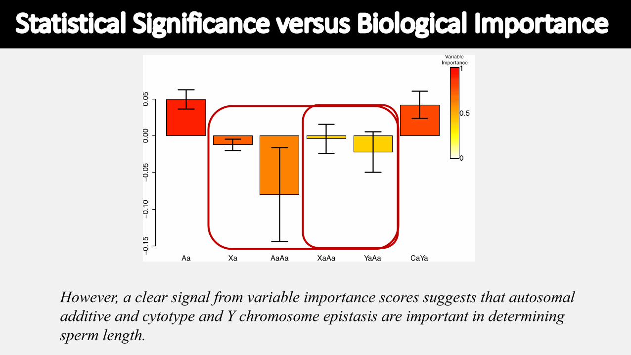
Statistical Significance versus Biological Importance
Aa Xa AaAa XaAa YaAa CaYa
ï0.15
ï0.10
ï0.05
0.00
0.05
0
0.5
1Variable
Importance
However, a clear signal from variable importance scores suggests that autosomal additive and cytotype and Y chromosome epistasis are important in determining sperm length.
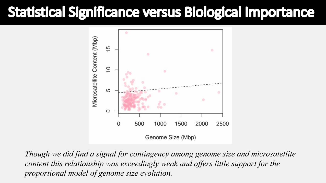
Statistical Significance versus Biological Importance
Though we did find a signal for contingency among genome size and microsatellite content this relationship was exceedingly weak and offers little support for the proportional model of genome size evolution.

Some vocabulary that will come upBalanceA balanced design has an equal sample size in each treatment and control group – balanced designs have the most power (usually).
Extreme TreatmentsBy using extremely high values of the treatment, we might be able to show an effect. We would have to consider whether these extreme values have biological relevance
FactorsA factor is a single treatment variable whose effects are of interest. An experiment can have more than one factor (light and humidity, for instance, would be two different factors). We sometimes wish to test multiple factors simultaneously, because they might interact
BlockingAn approach in experimental design to reduce the risk of confounding variables.

Block what you can, randomize what you cannot.
Treatment A
Control
Treatment B
Treatment C
Treatment A
Control Treatment B
Treatment C
Treatment A
ControlTreatment B
Treatment CTreatment A
Control
Treatment B
Treatment C
Plot 1 Plot 4Plot 3Plot 2

Example of Multiple Factors
• An experiment has multiple factors when you are interested in the effects of more than one variable.
• An example might be the role of genotype and environment on growth rate.
• Imagine there are two strains and you want to test their growth in two environments.
• A factorial design would require testing each strain in each environment for a total of four treatments
• This experiment would be called a full factorial design

Multiple factors and interactions

Precision
• It is possible to plan your experiment to achieve a desired level of precision
• The catch is that you have to know something about the expected standard deviation of your response variable
• The other catch is that you will often find the sample sizes needed to be shockingly high

Precision
• Formula for necessary sample size is test specific see page WS 447-449
• For comparing two means
Where n is the sample size required for each group and margin of error is the desired half width𝜎 is the standard deviation
• A smaller margin of error requires a larger sample size
• A larger standard deviation requires a larger sample size
𝑛 ≈ 8𝜎
𝑚𝑎𝑟𝑔𝑖𝑛 𝑜𝑓 𝑒𝑟𝑟𝑜𝑟
"

Power
• A more useful and common way to estimate the necessary sample size is to focus on power
• Power: the probability of rejecting the null hypothesis for a hypothesized difference in means
• Power calculations are often necessary
• When you fail to reject the null, was it because you had insufficient power to detect a reasonable departure?
• When you apply for a grant or institutional approval, the agency often wants to know that your experimental design will have the power to detect a difference if one exists.
Calculating Power
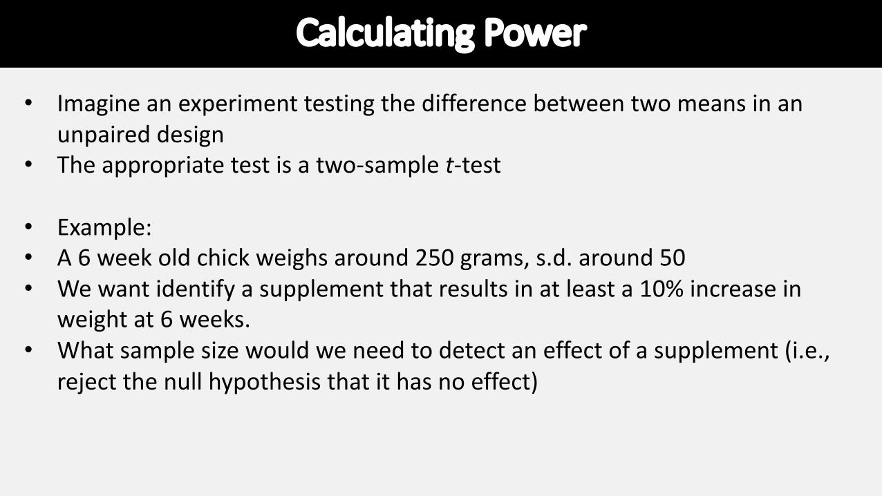
• Imagine an experiment testing the difference between two means in an unpaired design
• The appropriate test is a two-sample t-test
• Example:• A 6 week old chick weighs around 250 grams, s.d. around 50• We want identify a supplement that results in at least a 10% increase in
weight at 6 weeks.• What sample size would we need to detect an effect of a supplement (i.e.,
reject the null hypothesis that it has no effect)

Power for a Two-sample t-test
For a power of 0.8 (i.e., an 80 percent chance of rejecting the null hypothesis when it’s not true), I need a sample size of:
𝑛 = 16𝜎𝐷
!
𝑛 = 1650
275 − 250
!
D is the expected difference in means.
𝑛 = 64 For each treatment

Power for a Two-sample t-test
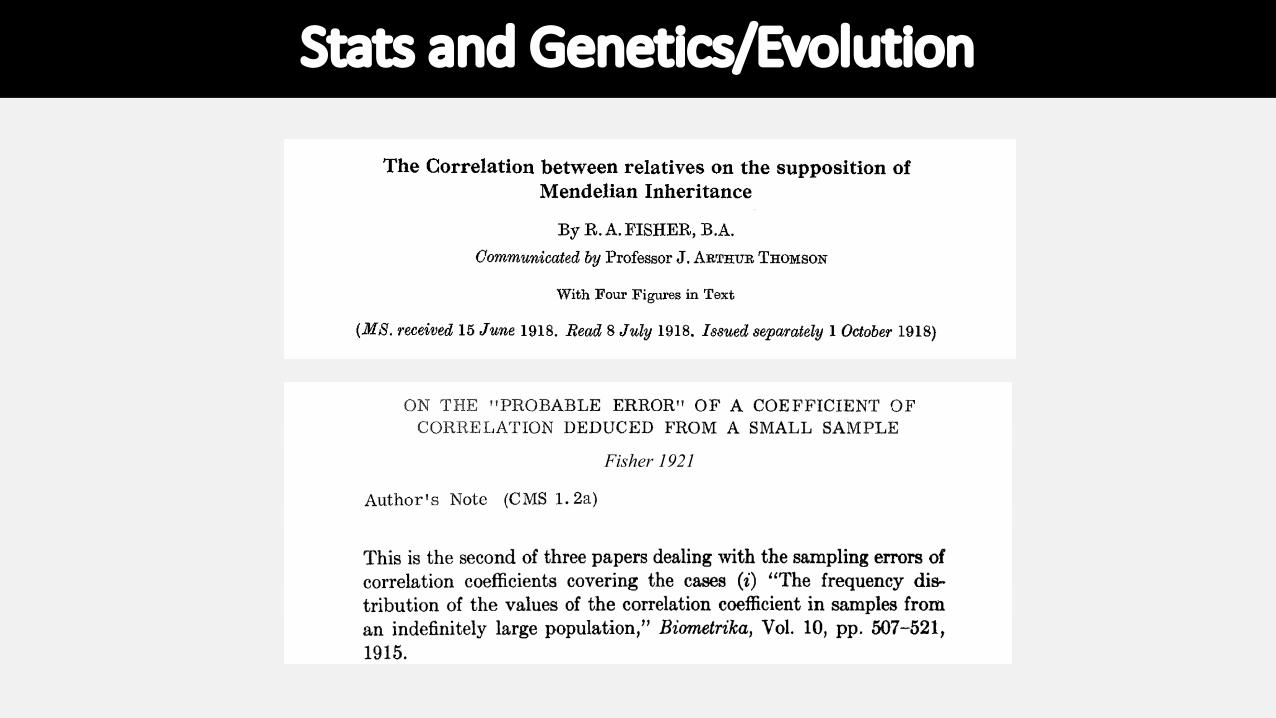
Stats and Genetics/Evolution
Fisher 1921

Analysis of Variance• Used to compare the means among more than two
groups
• If you are comparing three groups, for instance, you cannot just do three pair-wise t-tests – this approach would cause too many false positives
• ANOVA takes into account the fact that you are comparing multiple groups and controls the false positive rate.

Analysis of VarianceA B C
2 5 7
2 8 4
3 8 5
5 7 4 02
46
8
mea
sure
Group A Group B Group C
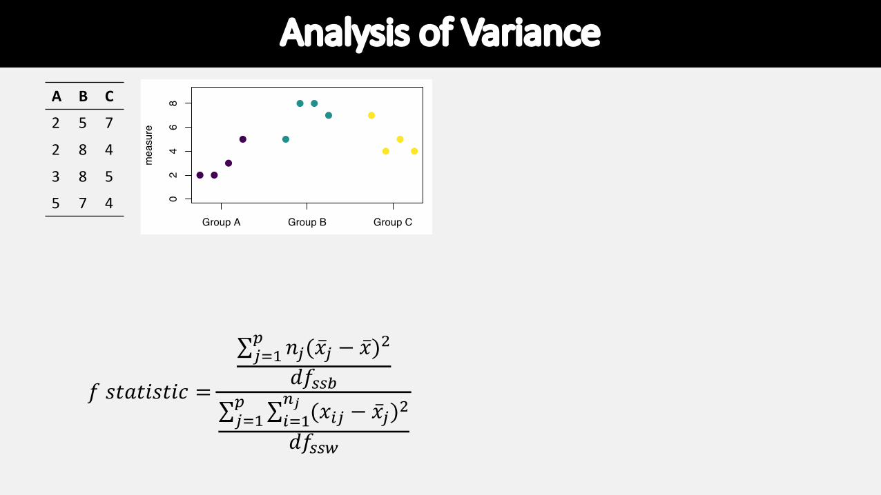
Analysis of Variance
𝑓 𝑠𝑡𝑎𝑡𝑖𝑠𝑡𝑖𝑐 =
∑!"#$ 𝑛!(�̅�! − �̅�)%
𝑑𝑓&&'∑!"#$ ∑("#
)! (𝑥(! − �̅�!)%
𝑑𝑓&&*
A B C
2 5 7
2 8 4
3 8 5
5 7 4 02
46
8
mea
sure
Group A Group B Group C
Analysis of Variance
𝑓 𝑠𝑡𝑎𝑡𝑖𝑠𝑡𝑖𝑐 =
∑!"#$ 𝑛!(�̅�! − �̅�)%
𝑑𝑓&&'∑!"#$ ∑("#
)! (𝑥(! − �̅�!)%
𝑑𝑓&&*
A B C
2 5 7
2 8 4
3 8 5
5 7 4 02
46
8
mea
sure
Group A Group B Group C
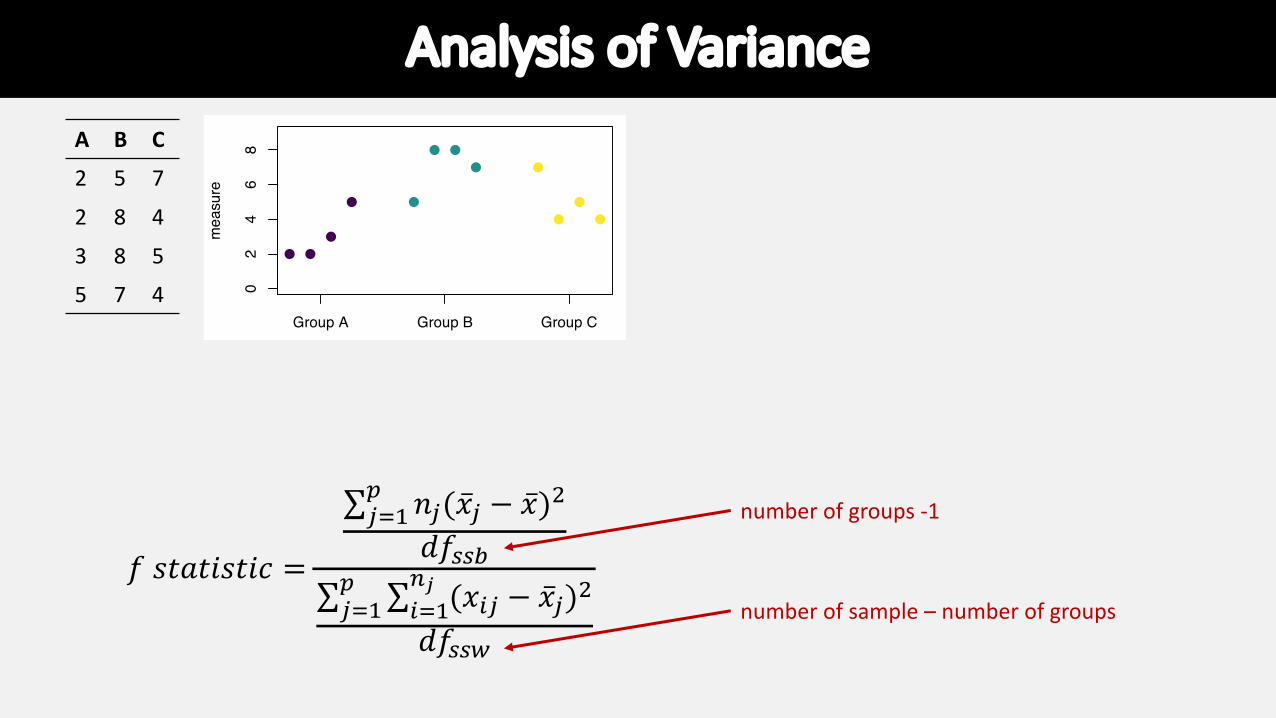
number of groups -1
number of sample – number of groups

Analysis of Variance
𝑓 𝑠𝑡𝑎𝑡𝑖𝑠𝑡𝑖𝑐 =
∑!"#$ 𝑛!(�̅�! − �̅�)%
𝑑𝑓&&'∑!"#$ ∑("#
)! (𝑥(! − �̅�!)%
𝑑𝑓&&*
A B C
2 5 7
2 8 4
3 8 5
5 7 4 02
46
8
mea
sure
Group A Group B Group C

Analysis of Variance
𝑓 𝑠𝑡𝑎𝑡𝑖𝑠𝑡𝑖𝑐 =
∑!"#$ 𝑛!(�̅�! − �̅�)%
𝑑𝑓&&'∑!"#$ ∑("#
)! (𝑥(! − �̅�!)%
𝑑𝑓&&*
A B C
2 5 7
2 8 4
3 8 5
5 7 4 02
46
8
mea
sure
Group A Group B Group C
02
46
8
mea
sure
Group A Group B Group C
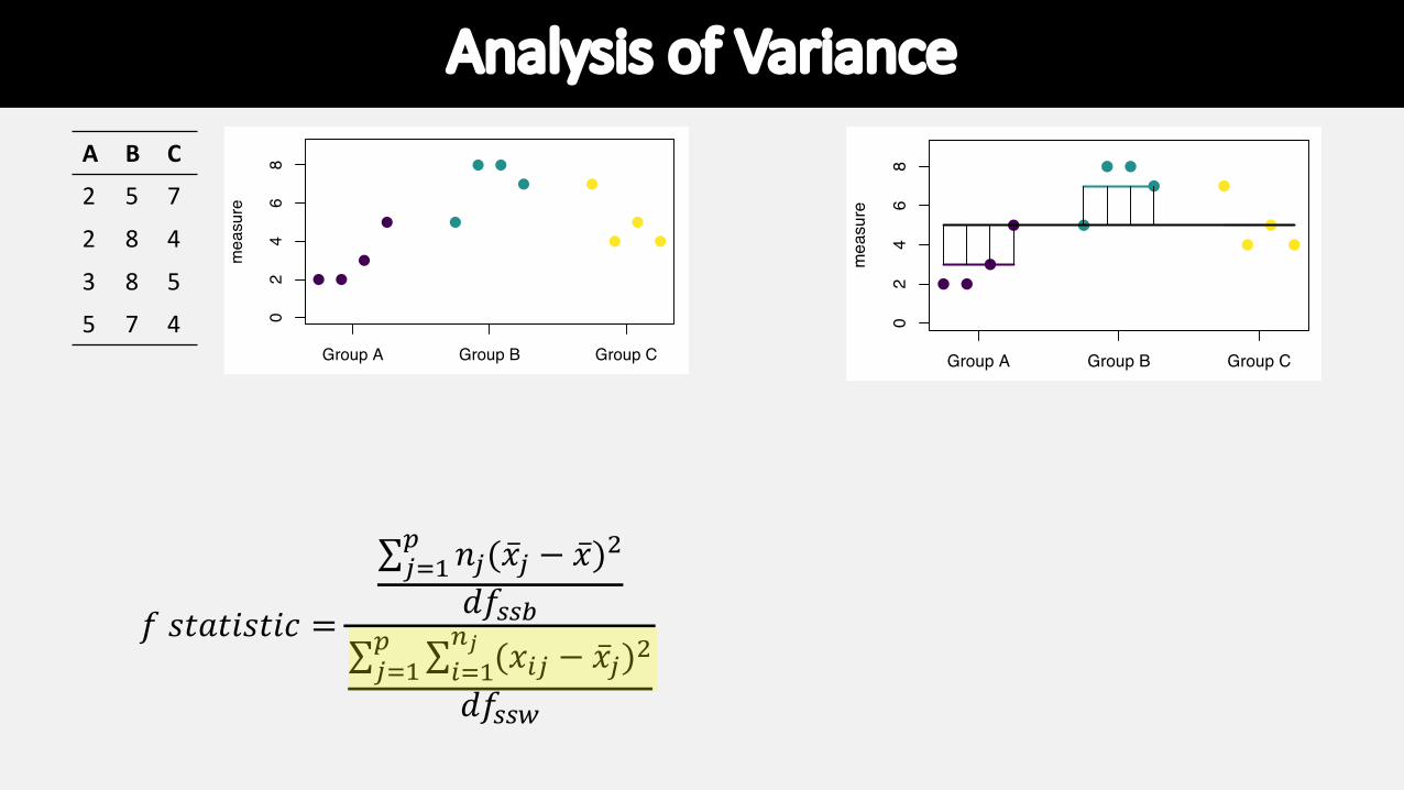
Analysis of Variance
𝑓 𝑠𝑡𝑎𝑡𝑖𝑠𝑡𝑖𝑐 =
∑!"#$ 𝑛!(�̅�! − �̅�)%
𝑑𝑓&&'∑!"#$ ∑("#
)! (𝑥(! − �̅�!)%
𝑑𝑓&&*
A B C
2 5 7
2 8 4
3 8 5
5 7 4 02
46
8
mea
sure
Group A Group B Group C
02
46
8
mea
sure
Group A Group B Group C
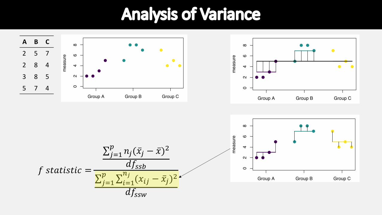
Analysis of Variance
𝑓 𝑠𝑡𝑎𝑡𝑖𝑠𝑡𝑖𝑐 =
∑!"#$ 𝑛!(�̅�! − �̅�)%
𝑑𝑓&&'∑!"#$ ∑("#
)! (𝑥(! − �̅�!)%
𝑑𝑓&&*
A B C
2 5 7
2 8 4
3 8 5
5 7 4 02
46
8
mea
sure
Group A Group B Group C
02
46
8
mea
sure
Group A Group B Group C
02
46
8
mea
sure
Group A Group B Group C

Running ANOVA in R
This significant result tells us that at least one of the groups of chickens have significantly different mean weights than other groups. (significant ANOVA result allows us to reject the null that they are all the same)

Running ANOVA in R

Post-hoc tests
If your ANOVA is significant, you may be interested in discovering which groups are different from one another
A variety of post-hoc comparisons of the means can be used
Fisher’s LSD• Least conservative test, basically uses t-tests to compare the means
Scheffe’s method• Performs all comparisons simultaneously, but has relatively low power
Tukey-Kramer method• A pair-wise method, like a t-test, but corrected for multiple comparisons

Post-hoc tests
anova and aov functions will both perform an ANOVA but the results are stored slightly differently. For this posthoc test we want the aov format

Interpreting post-hoc testsWhen we examine all the significantly different ones we can draw several conclusions:1) Chicks fed casein are significantly
heavier than those fed horsebean, linseed, and soybean.
2) Chicks fed horsebean are significantly lighter than those fed meatmeal, soybean, and sunflower.
3) Chicks fed sunflower are significantly heavier than those fed linseed or soybean.
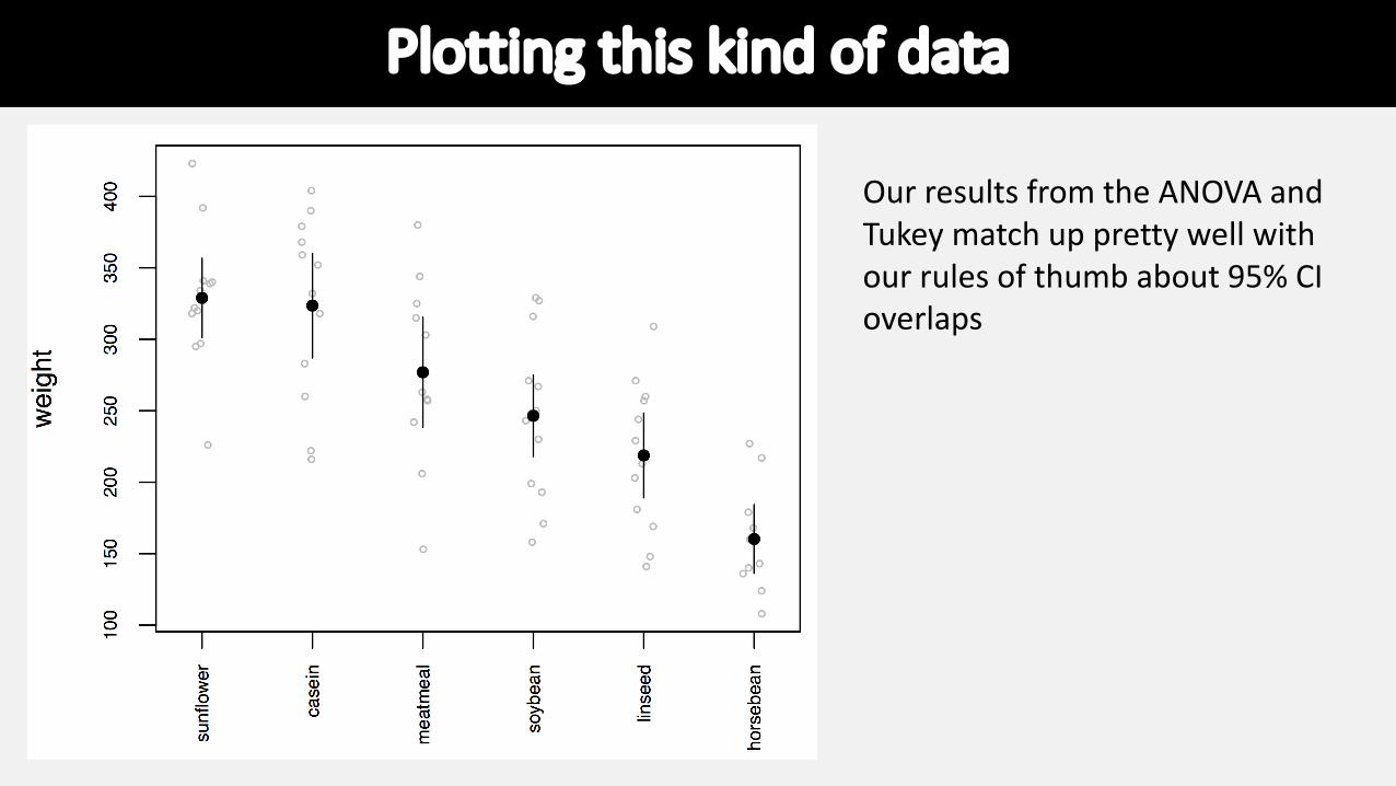
Plotting this kind of data
Our results from the ANOVA and Tukey match up pretty well with our rules of thumb about 95% CI overlaps

Example of code

Assumptions of the ANOVA
• The variable is normally distributed within each group
• The variance is the same in the different groups
• The design is balanced – you have the same sample size for each group
• But… ANOVA is fairly robust to violations of these assumptions

A Non-Parametric Alternative
• Kruskal-Wallis Test• Based on ranks• The multiple-group version of the Mann-Whitney U-test
R-implementation:
p-value suggests this test has lower powerthan ANOVA

A Non-Parametric post-hoc
• Dunn’s test – is the non-parametric equivalent of the Tukey
Not in base R need to install:install.packages(“dunn.test”, dependencies=TRUE)

ANOVA Summary• ANOVA is the foundation of essentially all tests comparing multiple
means• Don’t make it too complicated – the null hypothesis is simple: they are all
the same.• Post-hoc tests are important for determining which means are the source
of a significant ANOVA.• You can only justify a post-hoc test if the ANOVA is significant in the first
place.• Before applying ANOVA, check that your data fit the assumptions
(consider transforming the data lots of times this will be based on your biological knowledge because you will have insufficient data to say much about the observed distribution)

Correlation and Causation
The correlation is a foundational concept in the biological sciences
Pearson’s correlation coefficient:
𝑟 𝑋, 𝑌 =𝑐𝑜𝑣(𝑋, 𝑌)𝑠#𝑠$
Francis Galton1822 - 1911
Karl Pearson1857 - 1936
𝑐𝑜𝑣 𝑋, 𝑌 =∑("#) 𝑋( − 5𝑋 𝑌( − 5𝑌
𝑛 − 1 Shiny Example

Covariance and Correlation

Covariance and Correlation
Aver
age
num
ber o
fho
me
runs
per
gam
e
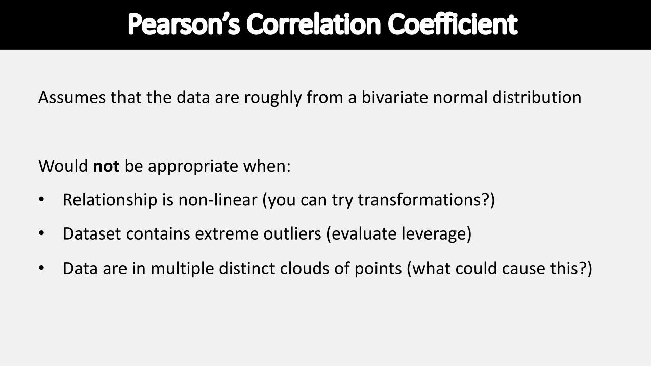
Pearson’s Correlation Coefficient
Assumes that the data are roughly from a bivariate normal distribution
Would not be appropriate when:
• Relationship is non-linear (you can try transformations?)
• Dataset contains extreme outliers (evaluate leverage)
• Data are in multiple distinct clouds of points (what could cause this?)
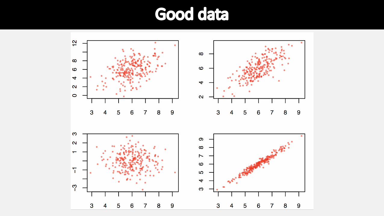
Good data

Bad data

Spearman’s Rank Correlation
An alternative to Pearson’s correlation coefficient for data that depart substantially from bivariate normality
Based on ranks

Correlation Summary
• Correlations are very important
• We are interested in correlations between values of treatments and response variables
• We are interested in correlations between various factors that could affect the response variable
• We need to think about correlations between explanatory variables and potentially confounding variables
• Many types of experiments call for the calculation and consideration of correlation coefficients


