

Master thesis I, 15 credits Master’s program in Economics, 120 credits
Spring term 2021
DETERMINANTS OF FOREIGN
DIRECT INVESTMENT IN
RWANDA
Renson Gatsinzi

1
ACKNOWLEDGEMENT
First and fore most, I thank the Almighty God for granting me life, protecting me, and for
His grace and love, without forgetting the wisdom and guidance throughout this study.
Appreciation and gratitude go to everyone who contributed towards my journey of this
research and through my entire education experience so far. However honorable mentions
are extended to the following:
I express my sincere appreciation to Umea University especially the department of
Economics for giving me the opportunity and supporting me to attain my education in
Sweden and to undertake this study.
To my family who have supported and encouraged me especially my Mum, I am very
grateful.
I extend my sincere gratitude to my supervisor Prof. Giovanni Forchini who guided and
advised me throughout this process of my research.
Finally, I thank all my friends and relatives who assisted me in various ways.
May God bless you all.
2
CONTENTS
1: INTRODUCTION ........................................................................................................................ 5
1.1: An overview of FDI in Rwanda ............................................................................................ 6
2. LITERATURE REVIEW ............................................................................................................. 7
2.1: Theoretical Literature ........................................................................................................... 7
2.2: Empirical Literature ............................................................................................................ 10
3.1: Description of data. .............................................................................................................. 14
3.2: Description of variables. ...................................................................................................... 14
3.3: Model specification .............................................................................................................. 15
3.4: Estimation procedures. ........................................................................................................ 16
3.4.1: Stationarity test. ............................................................................................................ 16
3.4.2: Selection of Optimal lag length. ................................................................................... 17
3.4.3: Cointegration test. ......................................................................................................... 17
3.4.4: Vector Error Correction Model (VECM). .................................................................. 18
4. EMPIRICAL RESULTS AND DISCUSSION ......................................................................... 19
4.1: Description statistics. ........................................................................................................... 19
4.2: Trend Analysis. .................................................................................................................... 20
4.3: Augmented Dickey-Fuller Test. .......................................................................................... 22
4.4: Selection of Optimal lag length ........................................................................................... 23
4.6.1: Vector Error Correction Model (VECM). .................................................................. 25
4.6.2: Two Long run equations. ............................................................................................. 27
4.7: VECM Post Estimation Diagnostic Tests........................................................................... 29
4.7.1: Test for Autocorrelation. .............................................................................................. 29
4.7.2: VECM Normality Test. ................................................................................................ 30
4.7.3: VECM Stability test. ..................................................................................................... 31
4.7.4: VECM Impulse Response Function (IRF). ................................................................. 32
5.1: Conclusions ........................................................................................................................... 34
5.3: Limitations and areas for further study. ........................................................................... 35
References. ....................................................................................................................................... 36

3
Abbreviations / Acronyms
FDI: Foreign Direct Investment
UNCTAD: United Nations Conference on Trade and Development
RDB: Rwanda Development Board
ADF: Augmented Dickey Fuller
MNC: Multinational Corporation
OLS: Ordinary Least Squares
SSA: Sub-Saharan Africa
M&A: Merger and Acquisition
BRICS: Brazil, Russia, India, China, South Africa
GDP: Growth Domestic Product
GMM: Generalized Method of Moments

4
ABSTRACT
This study attempts to examine the factors determining foreign direct investment in Rwanda
for the period 1970-2019. The study considers trade openness, market size, and government
expenditure as the determinants of FDI inflows. Time series analysis is used to examine the
significant determinants of FDI inflows in Rwanda. The study employs Johansen
cointegration test and VECM to establish a relationship between FDI and its determinants.
The findings indicate that trade openness (measured by sum of exports and imports as a ratio
of GDP) has a significant long run positive relationship with FDI. This implies that trade
openness is an important determinant of foreign direct investment in Rwanda. On the other
hand, market size and government expenditure are not significant determinants of FDI
inflows in Rwanda. The study concludes that openness of the Rwandan economy to a large
extent explains the direction of FDI inflows in the country and that foreign investors in
Rwanda are not market-seeking.
Key words: Foreign Direct Investment, VECM, Openness, Rwanda.

5
1: INTRODUCTION
Foreign direct investment (FDI) has become an economic buzzword as it has been perceived
by different people across time and space to play a pivotal role in the growth of economies
of both the developed and developing countries. Most developing economies lack enough
capital, and this has dramatically affected their economic growth and development. To
reverse the trend, policymakers have resorted to Investment as the panacea, especially foreign
direct investments, which will not only improve their desired gross domestic Investment and
savings but also boost the economic growth and development of these nations. FDI is
beneficial to the host economies in various ways such as job creation, transfer of knowledge,
technology spillovers, reduced prices by stimulating competition with local firms, among
others (Gichamo, 2012).
The term foreign direct investment refers to net inflows of Investment undertaken to acquire
a lasting management interest (10% or more of stock or voting rights) in a firm conducting
business in any economy other than the investor's home country. In general, an investment is
regarded as FDI when an investor establishes a business operation or acquires assets in a
foreign country. Such kinds of investments may either be in the form of "greenfield"
investment which is the establishment of a new business enterprise, or merger and acquisition
(M&A), which is investing in an already existing firm (Adeolu, 2007).
To attract more FDI, it is important that policymakers identify the factors that determine FDI
inflows in the economy.
Given the above reflections, this study seeks as its objective, to investigate and analyze the
determinants of FDI inflows in Rwanda using time series data from 1970 to 2019. Within the
context of this investigation, the study will answer two fundamental questions viz: “what are
the macroeconomic factors that drive FDI in Rwanda” and “does a reasonably stable long-
run relationship exist among FDI and these factors.”
Essentially, we consider this empirical journey important for the reasons outlined below:
6
1. Only a few studies exist on the determinants of FDI inflows in Rwanda. These studies have
largely used panel data modelling approaches dwelling on the comparative analysis of
Rwanda and other countries that may differ in economic standings.
2. Owing to the remarkably impressive growth of FDI inflows witnessed in the country in
the recent years, it becomes necessary to examine the macroeconomic drivers responsible for
such growth.
The rest of the thesis will be presented in four sections as follows: sections two and three
discuss literature review and methodology, section four contains data analysis and
discussion, section five consists of the conclusion and recommendations.
1.1: An overview of FDI in Rwanda
In the last two decades, the growth of Foreign Direct Investment (as well as Foreign Portfolio
Investment) in Rwanda has been very impressive. Statistical records reveal, for instance, that
FDI inflows increased from USD 382 million in 2018 to whopping USD 420 million in 2019,
and stocks were estimated at USD 2.6 billion at the end of 2019 (UNCTAD). Additionally,
in a report published by Rwanda Development Board (RDB) in 2019, the economy recorded
2.46 billion USD in Investment, which was a record high and of which 37% was in FDI. The
main sectors targeted by investors are Mining, Construction, and real estate, Infrastructure,
and Information and communication technologies, and according to Rwanda Development
Board (RDB) report, the major investing countries are Portugal, the UK, India, and the UAE.
The government of Rwanda has made a significant effort in attracting more FDI through
different measures to improve the investment climate in the country. Different supportive
mechanisms have been put in place, such as a one-stop center where registration of new
businesses and any information regarding Investment can be accessed, exchange platforms
between senior management and business leaders, among others. In 2015, a new investment
code was approved by the policymakers aiming at providing incentives to investors such as
a preferential corporate tax rate of 0% for an international company with its headquarters or
regional office in Rwanda, a preferential corporate tax rate of 15% for any investor, corporate
income tax holiday of up to 7 years, exemption from taxation on capital gains, exemption of

7
customs tax for products used in export processing zones, among others. The government
has also established various special economic zones such as the Kigali free zone and Kigali
industrial park free-trade zone. This has transformed Rwanda into one of the preferred
destinations for investors in recent years, and this is further evidenced by a report by world
bank 2020 in which Rwanda is ranked 38th out of 190 countries in the world in terms of ease
of doing business which makes it the highest-ranked country on the African continent.
Ameliorating Investment is seen as one of the strategies to guide the economy of Rwanda to
achieving its target of becoming a middle-income country by 2035 and a high-income
country by 2050.
2. LITERATURE REVIEW
Considerable amount of research on the determinants of FDI exist in the literature although
with differing conclusions ( see Asiedo, 2002 and Mijiyawa, 2015). An attempt is made in
this section to critically review some of these earlier studies under the broad headings of
theoretical and empirical literature.
2.1: Theoretical Literature
From the theoretical point of view, there are many scholars and schools of thought that have
come up with different theories to explain the phenomenon of FDI. Notably, in post-World
War II, some prominent theories have surfaced discussing this subject, such as Hymer (1976),
Aliber (1970), Kindleberger (1969), Knickberger (1973), Buckey and Casson (1976),
Wilhems & Witter (1998), Dunning (1974), Popovic & Calin (2014) among others. However,
there has been no consensus on a general theory that better explains FDI. These theories can
be examined from two economic perspectives, that is, the macroeconomic and
microeconomic points of view (Makoni, 2015).
The macroeconomic perspective is that FDI is a type of capital flow across borders, that is
between origin and host countries, and is captured in the balance of payments statement of
countries with the variables of interest being capital flows and stocks and revenues obtained
from those investments. The microeconomic perspective, on the other hand, relates to the
motives for investments across national boundaries, as seen from the investor's point of view
(Denisia, 2010).
FDI theories based on macroeconomic point of view include:

8
The capital market theory is also known as the "currency area theory." This theory was
based on the works of Aliber (1970), who claimed that foreign Investment came because of
imperfections in the capital market and FDI, in particular, because of differences in the
strength of currencies in the nations of origin and host nations. He argued that weaker
currencies in host nations compared to stronger currencies of the investing nations had higher
chances of attracting FDI compared to host nations with stronger currencies. Even though
the theory was proved consistent in developed countries like the USA, United Kingdom, and
Canada, it was criticized for not providing a sound explanation about Investment between
countries with equally strong currencies. Moreover, the theory did not explain the Investment
of Multinational Corporations (MNCs) from nations with weaker currencies in countries with
stronger currencies, with an example of MNCs from China and India investing in the UK and
USA (Nayak & Choudhury, 2014).
Location-based approach to FDI theory. The theory was developed by (Popovici & Calin,
2014), who articulated that the success of FDI among countries depended on factors such as
natural resource endowment, local market size, availability of labor, infrastructure, and
government policy in the country. The Authors went on to argue through their gravity
approach to FDI, which is a subsidiary to the location-based theory that FDI is more
successful if the countries involved are similar Geographically, Culturally, and economically.
Gravity variables such as size, level of development, distance, common language, and
additional institutional aspects like shareholder protection and trade openness were
considered as important determinants of FDI flows. However, the theory was criticized as
FDI flows are a more complicated theme than just similarities between countries and being
neighbours geographically may reduce transport costs but not essentially labor costs,
additionally sharing the same culture may not automatically mean increased profitability or
trade between two nations (Makoni, 2015).
Institutional FDI fitness theory. It was developed (Wilhems & Witter,1998), and the
theory focused on a country's ability to attract, absorb and retain FDI. The theory was based
on a pyramid with four fundamental pillars is Government, Market, education, and socio-
cultural fitness, which were regarded as the main determinants of the country's ability to
attract FDI inflows. The authors argued that it is not about how large the country is but how
able it is to use its macroeconomic factors such as government size, GDP, Inflation, market

9
size, among others, to fit in the required conditions to attract more FDI. The theory has been
tested empirically and proved relevant in the context of developing economies and Africa in
particular, where various studies have been conducted on FDI based on the above-mentioned
factors such as (Ho, 2011), (Amendolagine et al., 2013).
FDI theories based on microeconomic perspective discuss the motivations of FDI flows
from the investor's point of view, which implies that decision is made at the firm- level or
industry level.
Hymer (1976) developed firm-specific advantage theory in which he argued that the MNCs
decision to invest abroad is influenced by some sort of market power in the form of
advantages such as patent-protected superior technology, brand names, marketing and
management skills, economies of scale, and cheaper sources of finance (Nayak &
Choudhury, 2014). Hymer's theory laid a foundation in explaining international production,
and it was supported by scholars such as Kindleberger (1969) in his monopolistic power
model, Knickerbocker's (1973) oligopolistic theory of following the market leader, the
internalization theory of Buckley and Casson (1976) in an international context, among
others.
All microeconomic-based FDI theories are based on the same fundamental principle of the
existence of market imperfections. Dunning (1980), in his award-winning FDI theory,
combined these theories by introducing an eclectic paradigm that contextualized ownership,
internalization, and localizing advantages attained by MNCs as a three-tier masterpiece for
the engagement of FDI and international production. Dunning asserted that a firm must
satisfy three conditions simultaneously to take part in FDI.
Firstly, a firm must possess specific and exclusive ownership advantages such as trademarks,
patents, information, and technology over other rival firms to serve a particular market. Such
advantages would enable the firm to outcompete its rival in a foreign country.
Secondly, these advantages must be more profitable to the firm possessing them to use them
than to lease or sell them to a foreign firm in the form of licensing or management contracts.
Finally, suppose the above two conditions are met, the firm must benefit more from utilizing
the advantages in production in combination with other factor inputs like labor, natural
resources in a foreign country (Makoni, 2015).

10
To sum up, what has been discussed, having analysed different theories of FDI, there is no
single theory that comprehensively explains FDI. It is therefore up to the researcher to choose
which theory to base on while discussing FDI. However, Dunning's theory of the Electric
paradigm is the most recognized theory of FDI.
2.2: Empirical Literature
Several studies have been conducted to examine the determinants of FDI on the continental,
regional, and country levels. Different results were obtained, and varying conclusions were
made about what factors are more significant in determining FDI flows.
In one of the earliest studies on the subject in Africa, Morisset (2000) analyzed what
determines FDI in Africa. Using cross-section and panel data from 29 Sub-Sahara African
(SSA) countries, he asserted that FDI in African countries is determined by factors such as
natural resources, market size, economic growth, trade liberalization, macroeconomic
stability, political stability. The author also concluded that Africa could capture more
attention of foreign investors not only based on Natural resources or targeting the local
market size but also with the implementation of some visible and pro-active policy reforms
and improving their business climate.
In a contradicting fashion, Asiedu (2004) conducted a study on policy reforms and Foreign
Direct Investment in Africa. The author found out that, despite making some policy
improvements and reforming their institutions, improving their infrastructures, and
liberalizing their FDI regulatory framework, developing countries in Sub-Sahara Africa
(SSA) have continued to have a small share of FDI compared with developing countries in
other regions. She asserted that the cause for SSA being less competitive in attracting FDI is
due to mediocre reforms in comparison with the implemented reforms by other developing
countries in other regions.
In a similar study, Investigating 71 developing countries (32 Sub- Saharan African countries
and 39 non-Sub- Saharan African countries) (Asiedu, 2002), used cross-sectional data
analysis for the period1988-1997 and found that developing countries in SSA differ from
developing countries in other regions in what attracts FDI. According to the author, the
results showed that Trade openness attracts FDI to developing countries in both SSA and

11
non-SSA regions. However, the marginal effect of trade openness in SSA is lower. She
further illustrated that Infrastructure development and a higher return to Investment
positively influence FDI to non-SSA, but that is not the case for developing countries in SSA.
Using the fixed effect model, Suliman & Mollick (2009) investigated determinants of FDI
for 29 SSA countries using panel data collected between 1980 and 2003. They discovered
that GDP per capita growth, Human capital, openness, and infrastructure development have
a positive effect on FDI. On the other hand, political rights and civil rights, and liquidity size
of the market all exert a negative impact on FDI.
(Gichamo, 2012) carried out a study on the determinants of foreign direct investment inflows
in Sub - Saharan Africa, with panel data for the period 1986-2010 from a sample of 14
countries. The author employed pooled OLS, fixed effect, and random effect estimators, and
empirical results showed that gross domestic product, trade openness, Inflation, and a lag of
FDI are the most significant determinants of FDI inflows in Sub-Saharan Africa. The study
also found that the relationship between FDI inflows and telephone lines is insignificant. The
author also highlighted that the significance of variables is differing with countries.
Mijiyawa (2015) agreed with Gichamo (2012) in analyzing what drives FDI in Africa. The
author used panel data on 53 countries for the period 1970-2009 and employed a Fixed effect
estimator and Generalized Method of Moments (GMM) for analysis. The empirical results
showed that lagged FDI inflows, trade openness, political stability, market size, and return
on Investment are the significant determinants of FDI inflows to Africa. The author asserted
that it is not only about how big the country is but also the openness of the economy as well
as how stable the country is political. The study recommended the need to strengthen regional
integration to promote trade and a good political relationship among countries in the region.
For the case of developing countries, (Mottaleb & Kalirajan, 2010) examined the
determinants of FDI in developing countries. Considering factors like GDP size, GDP growth
rate, trade, aid, labor force, days required to start a business, growth rate of industrial value-
added, and the number of telephone users, the study used panel data on 68 low-income and
lower-middle-income countries from Africa, Asia, and Latin America for the period 2005-
2007. The results illustrated that, countries with larger GDP, higher GDP growth rate, a

12
higher proportion of international trade, and a more business-friendly environment attract
more FDI inflows. The study also concluded that small, developing countries could attract
more FDI by implementing more outward-oriented trade policies and providing a more
business-friendly environment to foreign investors.
Similarly, (Kumari & Sharma, 2017) analysed the determinants of FDI in developing
countries using panel data on 20 developing nations for the period 1990-2012. The study
considered factors such as market size, trade openness, infrastructure, Inflation, interest rate,
research and development, and human capital as the potential determinants of FDI and
utilized fixed effect and random effect estimators to analyze the data. The findings
established that market size, trade openness, and human capital are the significant
determinants of FDI in developing countries. The authors also asserted that market size is the
most important factor in attracting FDI in developing economies.
Using a holistic approach, (Jadhav, 2012) conducted a study to examine the economic,
institutional, and political determinants of FDI in Brazil, Russia, India, China, and South
Africa (BRICS). The study used panel data from 2000 to 2009 and employed panel unit root
and multiple regressions. The study considered market size, trade openness, and natural
resources as economic determinants, whilst macroeconomic stability, political stability,
government effectiveness, the rule of law, control of corruption, regulatory policy, and voice
and accountability as institutional and political determinants. The results established that
economic determinants are more significant than institutional and political determinants in
BRICS economies. The findings also indicated that market size and trade openness are
positive and significant determinants of FDI in BRICS whilst natural resources availability
is negatively related to FDI. According to the author, FDI in BRICS is more motivated by
market-seeking purposes and not resource-seeking.
In a similar study, Labes (2015) attempted to analyse FDI determinants in BRICS economies.
The study used panel data from 1992 to 2012. Considering factors such as Trade openness,
GDP per capita, population, exchange rate, and human capital as potential determinants, the
study employed pooled OLS, fixed effect, and random effect estimators. The findings found

13
that trade openness, GDP per capita, and exchange rate are the significant determinants of
FDI in BRICS economies. Narayanamurthy et al. (2017) examined the determinants of FDI
for BRICS countries using fixed effects and random effects estimators on panel data collected
from 1975 to 2007. The authors found that FDI in BRICS is determined by market size,
Industrial production, Labour cost, infrastructure facilities, Growth capital formation. On the
contrary, economic stability, growth prospects, and Trade openness have no significant
impact on FDI flows.
Meanwhile, Ang (2008) utilized the two-stage least squares methodology to analyze the
determinants of FDI in Malaysia using data collected from 1960-2005. According to the
Author, financial development, Infrastructure development, GDP growth, trade openness,
government size, and macroeconomic uncertainty all have a positive impact on FDI.
However, real exchange rates and taxation are negatively related to FDI.
Analyzing the determinants of FDI in Afghanistan, Wani & Tahiri (2017) used OLS on time
series data collected from 2005 to 2015, and the results revealed that total debt service, total
external debt, gross domestic product, and gross fixed capital formation positively affect FDI.
Inflation, on the other hand, negatively impacts FDI.
Dondashe & Phiri (2018) investigated the determinants of FDI for the South African
economy using time series data collected between 1994 and 2016. They deployed ARDL and
found that GDP per capita, Government size, real interest rate, and terms of trade are positive
determinants of FDI. On the other hand, the inflation rate negatively affects FDI.
(Habimana, 2018) examined the determinants of FDI in Rwanda. He established that GDP
as a proxy for the size of the economy and Inflation as a proxy for the stability of the economy
are significant factors in determining FDI inflows in Rwanda. The findings established that
GDP affected FDI positively whilst Inflation exerted a negative impact on FDI. The study
also found out that Exchange was not a significant determinant for FDI flows in Rwanda.
Sajilan et al. (2019), utilizing data on 42 countries, analyzed the determinants of FDI in
Organization of Islamic countries (OIC) countries. Panel data from 1996 to 2013 were
analyzed using fixed effect and random effect estimators, and the results showed that the size
14
of the economy, infrastructure, and trade openness exert a positive impact on FDI. On the
other hand, Institutional quality was negatively related to FDI, and the impact of Inflation on
FDI is mixed.
In summary, different researchers utilized various econometric methods such as Fixed and
random effect estimators on different kinds of data such as cross-section, panel, and time
series to analyze the determinants of FDI and achieved different conflicting results. However,
GDP, trade openness, and market size have been found to be the most significant
determinants of FDI by most of the studies.
3. RESEARCH METHODOLOGY
This chapter discusses the methodology used by the research to collect, process, and analyze
data. Annual time series data are used in this study, and an econometric model is developed
to examine how GDP per capita, trade openness, and Government Expenditure determine
Foreign Direct Investment (FDI) inflows in Rwanda in the period 1970 to 2019.
3.1: Description of data.
Annual time series data are collected on FDI net inflows, GDP per capita, trade openness,
and government expenditure for the period 1970 to 2019 to analyze the determinants of FDI
in Rwanda. The Source of the data on all variables was the World Bank (World Development
Indicators, 2020). More details about the relevant variables are explained in section 3.2
below.
3.2: Description of variables.
Foreign Direct Investment (FDI). It measures the net inflows of investment to acquire a
lasting management interest (10 percent or more of voting stock) in an existing enterprise in
any economy other than that of the investor. The series shows net inflows of investment to
an economy from the rest of the world as a percentage of GDP. The unit of measurement is
percent.

15
Gross Domestic Product per capita (GDPPC). It measures gross domestic product divided
by mid-year population. It determines the income earned per person in the economy. Other
factors being constant, GDPPC determines the demand of all individuals in the economy. In
this study, GDPPC is used as the proxy for market size, and a higher GDP per capita implies
a large market which is an incentive to attract foreign Investment. It is expected to be a
positive and significant determinant of FDI inflows. Some previous researchers used the
same variable, such as (Dondashe & Phiri, 2018). The unit for GDP per capita in this study
is USD millions (constant 2010).
Trade openness (TRDOP). It indicates the level of restrictions on trade activities in the host
economy. Investors prefer a more open economy which will allow them to export their
products to the markets abroad and import some intermediate goods that are used as raw
materials during production. This study used "Volume of Trade as a ratio of GDP," which is
measured by the sum of exports and imports of goods and services as a ratio of GDP to proxy
trade openness. It is expected to be a positive and significant determinant of FDI inflows.
(Mijiyawa, 2015), (Asiedu, 2002) and (Kumari & Sharma, 2017), among others, used the
same variable. The unit of measurement is percentage.
Government Expenditure (GE). It measures government consumption, investment, and
transfer payments. Expenditure on infrastructure such as roads, electricity, education acts as
an incentive to FDI. The study used general government final consumption expenditure as a
proxy for Government expenditure. Therefore, we expect a positive and significant
relationship between government expenditure and FDI. Some previous pieces of literature
utilized the same variable, such as (Adeolu, 2007) ( Norashida et al., 2016). The unit of
measure is USD millions (constant 2010).
3.3: Model specification
This study is built on the assumption that GDP per capita, trade openness, and Government
Expenditure determine Foreign Direct Investment (FDI) inflows. The groundbreaking work
of (Sims, 1980) laid a foundation for the study of how macroeconomic series are interrelated.
It is upon this background that economic theory developed Vector autoregressive (VAR)
model as an essential tool for analyzing empirically how economic variables are interrelated

16
in the short run. The phenomenon of VAR is further well described by (Levendis, 2018) in
his own words,
"If we take the notion of general equilibrium seriously, then everything in the economy is
related to everything else. For this reason, it is impossible to say which variable is exogenous.
It is possible that all variables are endogenous: they can all be caused and simultaneously be
the cause of some other variables".
Based on previous literature such as (Seetanah & Rojid, 2011), this study specified a vector
autoregressive model to analyze the relationship between FDI and its determinants in
Rwanda, and it is presented as:
𝑌𝑡 = 𝛽 + ∑ 𝛾𝑖𝑝𝑖=1 𝑌𝑡−1 + 𝑢𝑡 (1)
Where:
𝑌𝑡= (FDI, GDPPC, TRDOP, GE) represents a kx1 vector of endogenous variables
FDI= Foreign Direct Investment Net Inflows
GDPPC= Gross Domestic Product per capita
TRDOP= Trade Openness
GE= Government Expenditure
𝛾𝑖 (𝑖 = 1,2 3, … , 𝑝) represents a k x k matrix of autoregressive coefficients.
𝑢𝑡 It is a k x 1 vector of error terms that is identically and independently distributed.
3.4: Estimation procedures.
3.4.1: Stationarity test.
The stationarity test is essential when dealing with time-series data. In general, time series
are characterized by unit-roots, and therefore they are nonstationary. When a nonstationary
time series variable is regressed on another time series, it leads to a spurious regression. The
results from the regression might report significant coefficients with a remarkably high R2
even though there is no meaningful relationship between the two variables. These results
17
from such regression may be biased and misleading. A nonstationary time series is less
considered in forecasting as its behaviour is suited for a study only for the time under
consideration (Gujarati & Porter, 2009).
The presence of a unit root in a time series indicates that the series under study is
nonstationary. This study employed Augmented Dickey-Fuller (ADF) test to conduct the
stationarity test of the variables and determine their order of integration.
3.4.2: Selection of Optimal lag length.
The optimal number of lags is a requirement to carry out a cointegration test as well as to
estimate a well-established VAR model. Choosing the number of lags to include in the model
is difficult because the inclusion of too many lags may lead to loss of degrees of freedom and
risk facing a problem of multicollinearity whilst including too few lags may lead to
misspecification of the model and omission of important lagged variables. However, there
is no economic theory that explains the exact number of lags that should be in our model.
The choice of the optimal lag length is empirical, and there are various lag selection criteria
utilized in determining the optimal lag length for our VAR model, such as Final Prediction
Error (FPE), Schwarz Bayesian Information Criterion (SBIC), Akaike information criterion
(AIC), Hannan-Quinn information criterion (HQIC), Likelihood Ratio, etc. The most notable
and used among these are the Akaike information criterion (AIC) and Schwartz Bayesian
Information Criterion (SBIC), but the choice on which one to use between the two is
discretionary and exigent on the model, but the one with a lower value is preferred.
Furthermore, it is advisable to consider AIC when one has a small sample that is 60 or fewer
observations as it minimizes the chances of underestimating the true number of lags (Liew,
2006). This study employed AIC given that the number of observations is 50, and it has the
lowest value in comparison with the rest of the criteria.
3.4.3: Cointegration test.
Two or more nonstationary economic variables are cointegrated if they have a common
stochastic trend. This implies that a linear combination of them is stationary (Lutkepohl &
Kratzig, 2004). In which case, if variables are cointegrated, they have a long-run or
equilibrium relationship (Gujarati & Porter, 2009). There are two common approaches
utilized in cointegration testing. These are the Engle-Granger approach and the Johansen
18
cointegration test approach. Engle-Granger's approach is suitable for a univariate model with
only two variables, whereas the Johansen approach is well suited for a multivariate model as
it allows for simultaneous estimation of all the cointegrating relationships in the model under
study (Levendis, 2018). The fact that our model has four variables, this study utilized the
Johansen Cointegration test approach.
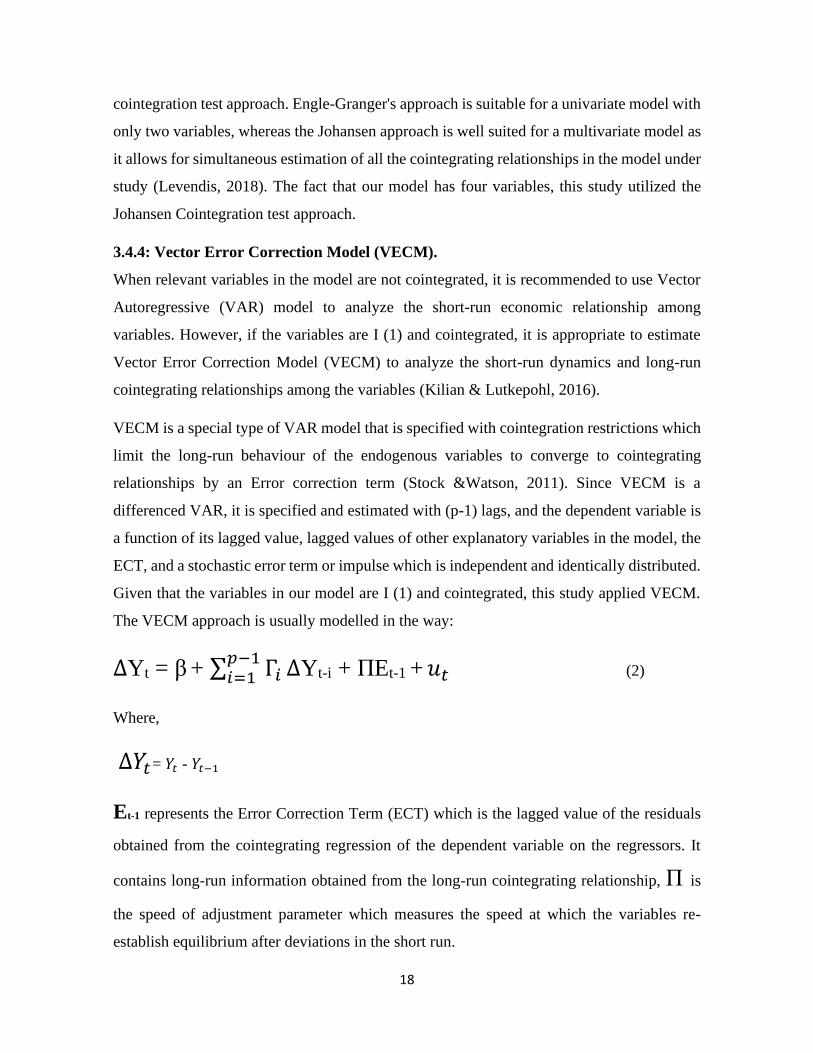
3.4.4: Vector Error Correction Model (VECM).
When relevant variables in the model are not cointegrated, it is recommended to use Vector
Autoregressive (VAR) model to analyze the short-run economic relationship among
variables. However, if the variables are I (1) and cointegrated, it is appropriate to estimate
Vector Error Correction Model (VECM) to analyze the short-run dynamics and long-run
cointegrating relationships among the variables (Kilian & Lutkepohl, 2016).
VECM is a special type of VAR model that is specified with cointegration restrictions which
limit the long-run behaviour of the endogenous variables to converge to cointegrating
relationships by an Error correction term (Stock &Watson, 2011). Since VECM is a
differenced VAR, it is specified and estimated with (p-1) lags, and the dependent variable is
a function of its lagged value, lagged values of other explanatory variables in the model, the
ECT, and a stochastic error term or impulse which is independent and identically distributed.
Given that the variables in our model are I (1) and cointegrated, this study applied VECM.
The VECM approach is usually modelled in the way:
∆Yt = β + ∑ Γ𝑖𝑝−1𝑖=1 ∆Yt-i + ПEt-1 + 𝑢𝑡 (2)
Where,
∆𝑌𝑡= 𝑌𝑡 - 𝑌𝑡−1
Et-1 represents the Error Correction Term (ECT) which is the lagged value of the residuals
obtained from the cointegrating regression of the dependent variable on the regressors. It
contains long-run information obtained from the long-run cointegrating relationship, П is
the speed of adjustment parameter which measures the speed at which the variables re-
establish equilibrium after deviations in the short run.

19
4. EMPIRICAL RESULTS AND DISCUSSION
4.1: Description statistics.
This section presents a summary of the data, and the results are reported in Table1. The
number of observations is 50 years from 1970 to 2019. The mean values of variables, Foreign
Direct Investment net inflows (FDI), Gross Domestic Product Per capita (GDPPC), Trade
Openness (TRDOP), and Government Expenditure (GE), is 1.166%, 467m USD, 34.6%, and
467 million USD, respectively. Interestingly, it is noted that mean values for all variables are
positive. This indicates that FDI inflows in Rwanda increased during most of the time under
study. The median values for FDI, GDPPC, TRDOP, and GE are 0.78%, 416.8m USD,
32.5%, and 304 million USD, respectively. Notably, the maximum and minimum values for
all variables indicate a large dispersion, and this is further shown by the high standard
deviation for all the variables, which indicates the deviation from their mean.
Table 1: Summary of descriptive statistics (1970-2019)
Variable Obs Mean Std. Dev. Median Min Max
FDI 50 1.166181 1.142797 .7879802 .0001327 3.807796
GDPPC 50 467.0239 158.0846 416.8239 219.6367 901.3044
TRDOP 50 34.62947 9.970366 32.5398 19.6842 71.0956
GE 50 467.08 423.13 304.32 481.53 1,770
Source: Author’s computation from Stata 16.4
For ease of interpretation and to account for influence of outliers that might characterize our
data, all variables are transformed into their natural logarithmic forms. Additionally,
transforming the series into logs ensures stable variance of the variables in the model. So, the
next tests will use the variables in their natural logarithm form. The variables will be:
lnFDI = Natural logarithm of FDI

20
lnGDPPC = Natural logarithm of GDPPC
lnTRDOP = Natural logarithm of TRDOP
lnGE = Natural logarithm of GE
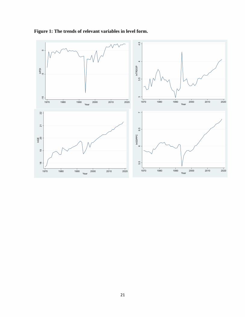
4.2: Trend Analysis.
Figure1 below shows the individual trends of all the relevant variables over the period of
study (1970-2019). The trends of all the variables show fluctuations in the same direction.
Additionally, there is a sharp decline in all the variables between 1990 and 1995. This is
reasonable because it was during the period of war, instability, and the infamous 1994
Genocide in Rwanda. However, after 1995 all the variables show a gradual increase which
implies that the economy was under-recovery and new policies being implemented. After the
year 2000 up to 2019, GDPPC, TRDOP, and GE are observed to be increasing at a high rate.
FDI, however, has been increasing but still volatile. It is noted that trends of relevant
variables in their levels presented in figure 1 show a tendency of fluctuating away from the
mean, suggesting that the mean is not constant; therefore, we suspect that all the variables
are nonstationary at levels. Figure 2, on the other hand, shows the first difference of all the
variables, and their trend shows a tendency to fluctuate around the mean, suggesting that
variables are stationary at their first difference.
Figures 1 and 2 depict the trends of the variables in their levels and at their first difference,
respectively.
21
Figure 1: The trends of relevant variables in level form.

22
Figure 2: The trends of the first difference of the relevant variables.
4.3: Augmented Dickey-Fuller Test.
To test the stationarity of the relevant variables and determine their order of integration,
Augmented Dickey-Fuller (ADF) was used, and the results are reported in Table4.2. The
number of lags was determined based on Ng and Perron (1995), with a maximum lag of 10
set based on the rule of thumb suggested by Schwert (1989). It is noted that FDI and TRDOP
were tested at lag 1, GDPPC was tested at lag 0, and GE was tested at lag 2. The test was
performed on all the variables in their natural logarithm (ln) form to account for the possible
presence of heteroskedasticity. The results from the test gave enough evidence to accept the
null hypothesis of unit root for lnFDI, lnGDPPC, lnTRDOP, lnGE, given that the t-statistics

23
in absolute value were less than the critical value at a 5% significance level, which means
that all the variables are nonstationary in their level form.
However, at their first difference, all the variables are stationary. This implies that all the
relevant variables are integrated of order one, that is, they are I (1).
Table 2: ADF Unit Root Test Results.
Variable ADF Statistics Order of Integration
Level First Diff Lags I(d)
lnFDI -2.571 -8.071*** 1 I (1)
lnGDPPC -1.649 -8.633 *** 0 I (1)
lnTRDOP -2.293 -7.114*** 1 I (1)
lnGE -2.588 -6.049 *** 2 I (1)
Source: Author's computation from Stata 16.4
Note: *** Implies significant at 1% level of significance. The critical values at 1%, 5% and
10% significance levels are -4.168, -3.508, and -3.185 respectively.
4.4: Selection of Optimal lag length
Before conducting a cointegration test and estimating the VAR model, it is appropriate to
select the number of lags to utilize in the estimation. Choosing the number of lags to include
in the model is difficult because the inclusion of too many lags may lead to loss of degrees
of freedom and risk facing a problem of multicollinearity whilst including too few lags may
lead to misspecification of the model and omission of important lagged variables. However,
there is no economic theory that explains the exact number of lags that should be included in
the model under study.
The choice of the optimal lag length is empirical, and there are various lag selection criteria
considered in determining the optimal lag length for our model, such as Final Prediction Error
(FPE), Akaike Information Criterion (AIC), Hannan-Quinn Information Criterion (HQIC),
and Schwartz and Bayesian Information Criterion (SBIC). Among all the Information

24
criteria, it is the choice of the researcher to choose which one to use. However, the criterion
with the lowest value is preferred. All the criteria suggested one lag as the optimal lag length
for the model under study, as shown by the results reported in Table4.3 below. This study
utilized AIC, given that it has the lowest value.
Table 3: Results for the lag selection test.
Lag LL LR FPE AIC HQIC SBIC
0 -
74.4961
NA .000357 3.41287 3.47244 3.57188
1 49.8661 248.72 3.2e-06* -1.29852* -1.00069* -.503463*
2 58.7226 17.713 4.5e-06 -.987939 -.451836 .443172
3 74.1468 30.848 4.8e-06 -.962906 -.188535 1.10425
4 94.3093 40.325* 4.3e-06 -1.14388 -.131246 1.55932
Source: Author’s computation from Stata 16.4
4.5: Johansen Cointegration Test.
After establishing that all the variables are integrated of order one and determining the
optimal lag length, it is appropriate to test for cointegration to discover if the relevant
variables have a long-run relationship. Johansen cointegration test was employed to
determine the possible number of cointegrating equations in the model. The decision criteria
is that Trace statistics and max statistics are compared to their respective 5% critical value.
If the trace statistics and max statistics are greater than critical value, null hypothesis of (no
cointegration) is rejected and vice versa.
The optimal lag length of one suggested by AIC in Table 3 above was utilized in the test, and
the results are reported in Table 4 below. From the results, both Trace statistics and Max
statistics suggested two cointegrating equations in the model. This indicates that there is a
long-run or equilibrium relationship among the relevant variables in the model under
consideration.

25
Table 4: Johansen Cointegration Test results.
Maxi.
Rank
Parms
Trace
Statistics
5% Crit.
Value
Max Statistic
5% Crit. Value
0 4 90.3725 47.21 45.185 27.07
1 11 35.8540 29.68 27.8762 20.97
2 16 7.9778* 15.41 7.8540 14.07
3 19 0.1238 3.76 0.1238 3.76
4 20
Source: Author's computation from Stata 16.4
4.6.1: Vector Error Correction Model (VECM).
This section intends to analyse the short-run dynamics in the relevant variables in the model.
The most important part of the short-run analysis of a VECM is the Error Correction Term
(ECT) which estimates the speed at which variables return to equilibrium in case of
deviations in the short run. More so, it indicates that the deviations of the variables from the
equilibrium are gradually corrected through the adjustments. It is very important when the
coefficient of the ECT is negative and statistically significant.
The ECTs are denoted as ECT1 and ECT2 for every variable in the model, and the results
are shown in Table 5. The results are explained in detail below, with much emphasis on the
FDI model.
VECM is specified and estimated with (p-1) lags, the optimal lag length (p) for the model
under study was 1 as suggested by AIC in optimal lag selection test above. For this reason,
the results from VECM estimation did not generate parameters for short run dynamics of the
relevant variables in the model. Only the coefficients estimating speed of adjustments to re-
establish equilibrium in case of deviations in the short run were generated. However, this is

26
not problematic because the objective of the study is to establish a long run relationship
among the variables in the model. The speed of adjustment for all the relevant variables is
discussed in detail below.
Foreign Direct Investment (FDI).
The coefficient for ECT1 has a negative sign and is statistically significant. The speed of
adjustment is approximately 74% per year towards the equilibrium. This implies that FDI has
a relatively high speed of adjustment to converge to the equilibrium in case of any
unanticipated shocks or innovations. On the other hand, the coefficient for ECT2 indicates
that the speed of adjustment for FDI is 227% per year. However, it has a positive sign and is
statistically insignificant.
Gross domestic product per capita (GDPPC)
The results show that the coefficient for ECT1 is 0.009, which implies that the speed of
adjustment for GDPPC is approximately 0.9% per year towards equilibrium. It is positive
and statistically insignificant. Whilst the coefficient of ECT2 illustrates that the speed of
adjustment for GDPPC is 12.7% every year towards equilibrium.
Trade openness (TRDOP)
The coefficient of ECT1 shows that TRDOP adjusts at a speed of 2.5% per to return to
equilibrium, whilst ECT2 indicates that the speed of adjustment for TRDOP towards
equilibrium is 29.7% per year. However, both coefficients are positive and statistically
insignificant.
Government expenditure (GE)
Empirical results indicate that from the coefficient of ECT1, the speed of adjustment for GE
is 0.06% per year towards equilibrium, while the coefficient of ECT2 illustrates that GE
adjusts at 6.2% per year to return to equilibrium in case of a shock in the independent
variables. However, the coefficients are statistically insignificant.

27
Table 5: VECM Estimation results.
Coef. Std. Err. P-value
∆lnFDI
ECT1 -.7455105 .1859339 0.000
ECT2 2.278555 1.637923 0.164
∆lnGDPPC
ECT1 .0091554 .0145099 0.528
ECT2 -.2956986 .1278197 0.021
∆lnTRDOP
ECT1 .025997 .0260177 0.318
ECT2 .2974828 .2291942 0.194
∆lnGE
ECT1 -.006356 .0316 0.841
ECT2 -.0629743 .2783697 0.821
Source: Author’s computation from Stata 16.4
The fact that all the relevant variables are nonstationary at levels and only become stationary
after the first difference and they are cointegrated puts the focus of this study to investigate
the long-run relationship among the variables in the model. The next section describes the
long-run relationships in the model under study.
4.6.2: Two Long run equations.
Levendis (2018) suggested that the most important part of the VECM economically is the
cointegrating equations. It indicates the cointegrating relationships among the variables of
interest. From Table 6 below, _ce1 and _ce2 show that there are two cointegrating equations
in the model.

28
The Johansen identification scheme placed four constraints on the parameters in the two
cointegrating equations. In the first cointegrating equation, lnFDI was normalized to one
while lnGDPPC was normalized to zero implying that market size does not have a long run
relationship with FDI inflows in Rwanda. Similarly, in the second cointegrating equation,
lnFDI was normalized to zero whereas, lnGDPPC was normalized to one.
Table 6: Normalized Cointegration Coefficients.
_ce1 Beta Coef. Std. Err. P-value
lnFDI 1 .
lnGDPPC 0 (Omitted)
lnTRDOP -6.20824 1.440296 0.000
lnGE .3950569 .4227777 0.350
_cons 14.36179 .
_ce2
lnFDI 0 (Omitted)
lnGDPPC 1 .
lnTRDOP -1.058901 .1881433 0.000
lnGE -.1457104 .0552267 0.008
_cons .4517458 .
Source: Author's computation from Stata 16.4
It is noted that all the variables are in log form, so the coefficients can be interpreted as long-
run elasticity.
The first long run equation is therefore presented as:
lnFDI = 0.62lnTRDOP – 0.395lnGE – 14.36 (6)

29
This implies that Foreign Direct Investment is a function of Trade Openness and Government
expenditure.
The positive cointegrating coefficient for trade openness is 0.62, indicating a positive
relationship between trade openness and FDI inflows, implying that a 1% increase in Trade
openness increases FDI inflows by 0.62%. The results confirm the prior expectations, and
this implies that trade openness is an important factor in attracting FDI into Rwanda.
The empirical results show a negative relationship between government expenditure and FDI
inflows, meaning a 1% increase in government expenditure results in a decrease in Foreign
Direct Investment by 0.39%. Though the coefficient is statistically insignificant, and the
result is inconsistent with the prior expectations.
The second long run equation is presented as:
lnGDPPC = 1.059lnTRDOP + 0.146lnGE – 0.45 (7)
This means that GDP per capita is a function of trade openness and government expenditure.
The coefficient 1.059 is positive, which implies a positive relationship between trade
openness and market size in Rwanda. When trade openness increases by 1%, GDP per capita
increases by 1.059%.
According to the results, the cointegrating coefficient for government expenditure is 0.146
illustrating a positive relationship between government expenditure and market size,
meaning that a 1% increase in government expenditure increases market size by 0.146%.
4.7: VECM Post Estimation Diagnostic Tests.
Post-estimation tests are conducted to ensure that the fitted model is valid. These tests are
intended to check stochastic properties of the model, such as normal distribution of the
residuals, presence of serial correlation in the error terms, stability of the model.
4.7.1: Test for Autocorrelation.
It is essential to test for serial correlation in the residuals after estimating a VECM. We
conducted Lagrange -multiplier test, and the null hypothesis is that there is no autocorrelation
at lag order d, and the results are reported in Table 7.
30
Table 7: Lagrange- Multiplier Test Results.
Lag chi2 df Prob > chi2
1 22.5586 16 0.12605
2 24.7558 16 0.07425
H0: no autocorrelation at lag order
According to the results, we cannot reject the null hypothesis, given that the p-values at lags
1 and 2 are greater than 0.05. We conclude that the model has no problem of autocorrelation.
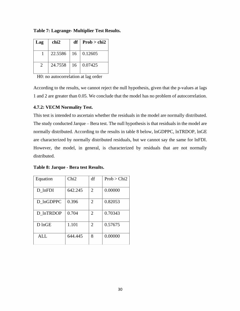
4.7.2: VECM Normality Test.
This test is intended to ascertain whether the residuals in the model are normally distributed.
The study conducted Jarque – Bera test. The null hypothesis is that residuals in the model are
normally distributed. According to the results in table 8 below, lnGDPPC, lnTRDOP, lnGE
are characterized by normally distributed residuals, but we cannot say the same for lnFDI.
However, the model, in general, is characterized by residuals that are not normally
distributed.
Table 8: Jarque - Bera test Results.
Equation Chi2 df Prob > Chi2
D_lnFDI 642.245 2 0.00000
D_lnGDPPC 0.396 2 0.82053
D_lnTRDOP 0.704 2 0.70343
D lnGE 1.101 2 0.57675
ALL 644.445 8 0.00000

31
4.7.3: VECM Stability test.
The stability test for VEM is conducted to check that the model is unbiased and that we have
correctly specified the number of cointegrating equations in the model. To check the stability
condition, the companion matrix of a VECM with K variables and r integrating equations has
K-r unit eigenvalues. The model is stable if the moduli of the remaining r eigenvalues are
strictly less than one. However, there is no general distribution theory to back up the
statement (Brinkgreve & Kumarswamy, 2008).
Table 9: Eigenvalue Stability Condition.
Eigenvalue Modulus
1 1
1 1
.3733731 .373373
.1156825 .115682
The VECM specification imposes 2 unit moduli.
Figure 3: Roots of the companion matrix.

32
The results reported in Table 9 show that the specified VECM imposes 2 unit moduli on the
companion matrix and the remaining eigenvalues are less than 1. It is further observed on the
footer in Figure 3 that none of the remaining eigenvalues are closer to the unit circle. This
implies that the model meets the stability condition and therefore it is robust.
4.7.4: VECM Impulse Response Function (IRF).
IRF describes the effect of impulses, innovations, or shocks in one time series variable on
another variable after a given number of periods (steps). It shows the responsiveness of a
dependent variable in case of unanticipated shock in the independent variable, the sign of the
effect, and how long it takes for the dependent variable to respond to the shock.
Unlike shocks in VAR models which vanish over time, shocks in VECM do not diminish
and therefore are either permanent or transitory. This study estimated a VECM impulse
response function to examine the impact of shocks in trade openness, market size, and
government expenditure on Foreign Direct Investment in Rwanda for 15 years to check the
persistence of the shock in the long run, and the results are shown in figure 4 below. The
response is statistically significant if the responses are above the zero line, and it is
statistically insignificant if it is below the zero line (Ahmad, 2015).

33
Figure 4: Results of the Impulse Response Function of VECM.
According to the results in figure 4, a one-time shock in trade openness has a permanent
positive effect on foreign direct investment inflows in Rwanda, whilst a shock in government
expenditure exerts a negative impact on FDI inflows in Rwanda. On the other hand, a shock
in market size has a transitory effect on foreign direct investment inflows in Rwanda. It is
further noted from figure 4 that FDI responds immediately to the shocks in the explanatory
variables because the change starts in the first period.
From figure 4 FDI responds in a mixed manner to a shock in GDP per capita. The response
is negative in the first two years, it increases after that up until the fourth year and the impact
of the shock stabilizes after four years. However, it noted from the figure that the response is
minimal because the deviation of the graph from zero line is small both positively and
negatively.
The response of FDI inflows to a shock in government expenditure is negative and decreasing
although it stabilizes after two years. This is surprising given that an increase in government
expenditure is expected to have a positive impact on FDI inflows. This could be because the

34
government of Rwanda spends on activities that are not related to promotion of FDI.
However, the response is statistically insignificant as it is below the zero line.
Foreign Direct Investment responds positively to a shock in trade openness. From the
beginning, a shock in trade openness leads to a rapid increase in FDI inflows. When the
economy is more liberalized, the country is engaged in more international trade activities and
increase foreign investors are induced to invest more.
5. Conclusions and recommendations
This section presents a summary of findings and conclusions from the study,
recommendations to the policymakers, as well as suggestions for further studies about the
same subject that would yield better outcomes.
5.1: Conclusions
This study provided a time series analysis of the determinants of FDI in Rwanda from 1970
to 2019. Variables such as trade openness, market size and government expenditure were
considered by the study as the potential determinants of FDI inflows in Rwanda. Johansen
cointegration test and VECM were employed to establish the long run relationship between
FDI and its determinants. Results from a unit root test using ADF established that all the
variables were nonstationary at levels but stationary in their first difference. This implies that
all the variables are integrated of order one. It was also shown that variables in the model
were cointegrated, suggesting a long-run equilibrium relationship among the relevant
variables.
Findings from VECM model showed that there is a long-run positive relationship between
trade openness which is measured by the sum of exports and imports as a ratio of GDP and
FDI, implying that trade openness is an important factor in determining FDI in Rwanda.
These results indicate that foreign investors in Rwanda are attracted by openness of the
economy and the good exporting policy in the country. On the other hand, market size is
found not to be a significant determinant of FDI inflows in Rwanda. This could be related to
the small population size of the country, which was 12.63 million in 2019. This implies that
MNCs in Rwanda are not market-seeking. Similarly, government expenditure is reported not

35
to be an important determinant of foreign direct investment in Rwanda despite a sound
theoretical argument.
Furthermore, results also established that approximately 74% of discrepancies between
equilibrium and short-run FDI are corrected per year.
Results from IRF showed that a shock in trade openness had a permanent positive impact on
FDI inflow in Rwanda, whilst a shock in government expenditure had a permanent negative
effect on FDI. A shock in market size, on the other hand, had a transitory impact on FDI
inflows.
5.2: Recommendations.
The results suggested that trade openness is a very important factor in determining FDI
inflows in Rwanda. This implies that the policymakers should formulate and implement more
policies aimed at liberalizing the economy and making it more open to international trade to
induce more foreign investors into the country. Engaging in more economic integrations
would be a good strategy to make the economy more involved in international trade there by
opening more doors for FDI inflows.
5.3: Limitations and areas for further study.
The study was restricted to a few variables, especially on the economic determinants of FDI,
due to the availability of data. Further studies with the inclusion of political and institutional
determinants may yield better results.
Conducting a similar study using different proxies for variables like government expenditure
and market size may provide different and significant results.

36
References.
Adeolu, B. A. (2007). FDI and Economic Growth: Evidence from Nigeria. In AERC
ResearchPaper(Vol.165,IssueApril).
https://publications.aercafricalibrary.org/bitstream/handle/123456789/22/RP_165.pdf?
sequence=1&isAllowed=y
Ahmad, F. (2015). Determinants of savings behavior in Pakistan: Long run-short run
association and causality. Timisoara Journal of Economics and Business, 8(1), 103-136.
Aliber, R.Z. 1970, "A theory of direct foreigninvestment", The international corporation, pp.
17-34.
Amendolagine, V., Boly, A., Coniglio, N. D., Prota, F., & Seric, A. (2013). FDI and Local
Linkages in Developing Countries: Evidence from Sub-Saharan Africa. World
Development, 50, 41–56. https://doi.org/10.1016/j.worlddev.2013.05.001
Ang, J. B. (2008). Determinants of foreign direct investment in Malaysia. Journal of Policy
Modeling, 30(1), 185–189. https://doi.org/10.1016/j.jpolmod.2007.06.014
Asiedu, E. (2002). On the determinants of foreign direct investment to developing countries:
Is Africa different? World Development, 30(1), 107–119.
https://doi.org/10.1016/S0305-750X(01)00100-0
Asiedu, E. (2004). Policy Reform and Foreign Direct Investment in Africa: Absolute
Progress but Relative Decline. In Development Policy Review (Vol. 22, Issue 1).
Overseas Development Institute. www.avmedia.at/nepad/
Brinkgreve, R. B. J., & Kumarswamy, S. (2008). Reference Manual Reference Manual. In
Technology (Vol. 1, Issue November).
Buckley P. and Casson M. (1976), “The Future of the Multinational Enterprise”, London,

37
MacMillan.
Denisia, V. (2010). Dunning OLI paradigm theory. European Journal of Interdisciplinary
Studies, 2(2), 104–110.
Dondashe, N., & Phiri, A. (2018). Munich Personal RePEc Archive Determinants of FDI in
South Africa : Do macroeconomic variables matter ? Munich Personal RePEc Archive,
83636.
Dunning, J.H. 1980, "Toward an eclectic theory of international production", The
International Executive, vol. 22, no. 3, pp. 1-3.
Dunning, J.H. 1980, "Towards an eclectic theory ofinternational production: some empirical
tests",
Journal of International Business Studies, vol. 11, no.1, pp. 9-31.
Gichamo, T. Z. (2012). Determinants of Foreign Direct Investment Inflows to Sub-Saharan
Africa: a panel data analysis. 2012.
Habimana, S. (2018). Analysis of the Determinants of Foreign Direct Investment in Rwanda
( Period of 1970-2010 ): Econometric Approach. 6, 1–26.
Ho, C. S. F. (2011). Macroeconomic and Country Specific Determinants of FDI Panel Error
Correction Model View project Event Study View project. September 2011.
https://www.researchgate.net/publication/278390346
Hymer, S.H. 1976, The international operations ofnational firms: A study of direct foreign
investment,MIT press Cambridge, MA.
Jadhav, P. (2012). Determinants of foreign direct investment in BRICS economies: Analysis
of economic, institutional and political factor. Procedia - Social and Behavioral
Sciences, 37, 5–14. https://doi.org/10.1016/j.sbspro.2012.03.270
Kindelberger C. (1969), “American Business Abroad: Six lectures on direct investment”,
NewHaven: Yale University Press.
Knickerbockers F. (1973), “Oligopolistic reaction and multinational enterprise”,
ThunderbirdInternational Business Review, 15(2), 7-9.

38
Kumari, R., & Sharma, A. K. (2017). Determinants of foreign direct investment in
developing countries: a panel data study. International Journal of Emerging Markets,
12(4), 658–682. https://doi.org/10.1108/IJoEM-10-2014-0169
Labes,S.-A.(2015).FDI Determinants in BRICS. VII(2), 296–308.
http://ceswp.uaic.ro/articles/CESWP2015_VII2_LAB.pdf
Levendis, J. D. (2018). Time Series Econometrics: Learning Through Replication. In
Springer Texts in Business and Economics. https://doi.org/10.1007/978-3-319-98282-
3%0Ahttp://link.springer.com/10.1007/978-3-319-98282-3
Liew, V. K. (2006). Which Lag Length Selection Criteria Should We Employ. Economics
Bulletin, 3(33), 1–9.
Lütkepohl, H. & Krätzig, M.,. (2004). Applied time series econometrics (No. 04; HA30. 3,
A6.). Cambridge/MA: Cambridge University Press.
Makoni, P. L. (2015). 10-22495_Rgcv5I2C1Art1.Pdf. 5(2), 77–83.
Mijiyawa, A. G. (2015). What Drives Foreign Direct Investment in Africa? An Empirical
Investigation with Panel Data. African Development Review, 27(4), 392–402.
https://doi.org/10.1111/1467-8268.12155
Morisset, J. (2000). Foreign Direct Investment in Africa: Policies Also Matter (Google
eBook). May, 20.
http://books.google.com/books?hl=en&lr=&id=rRzktbMMWmQC&pgis=1
Mottaleb, K. A., & Kalirajan, K. (2010). Determinants of Foreign Direct Investment in
Developing Countries: A Comparative Analysis. Margin, 4(4), 369–404.
https://doi.org/10.1177/097380101000400401
Narayanamurthy, V., Sridharan, P., & Rao, K. C. sekhara. (2017). Determinants of FDI in
BRICS Countries: A panel analysis. Int. Journal of Business Science and Applied
Management, 5(3). http://www.sussex.ac.uk/spru/
Nayak, D. & Choudhury, R.N. 2014, A selective review of foreign direct investment theories,
(No.143), ARTNeT Working Paper Series.

39
Othman, Norashida; Yusop, Zulkornain; Andaman, Gul; Ismail, M. M. (2016). Impact of
Government Spending on Small. International Journal of Business and Society, 1(2),
41–56.
Popovici, O.C. & Călin, A.C. 2014, "FDI theories. Alocation-based approach", Romanian
EconomicJournal, vol. 17, no. 53, pp. 3-24.
Sajilan, S., Islam, M. U., Ali, M., & Anwar, U. (2019). The determinants of FDI in OIC
countries. International Journal of Financial Research, 10(5), 466–473.
https://doi.org/10.5430/ijfr.v10n5p466
Seetanah, B., & Rojid, S. (2011). The determinants of FDI in Mauritius: a dynamic time
series investigation. African Journal of Economic and Management Studies, 2(1), 24–
41. https://doi.org/10.1108/20400701111110759
Sims, C. A. (1980). Macroeconomics and Reality. Econometrica, 48(1), 1.
https://doi.org/10.2307/1912017
Stock, J. H., & Watson, M. W. (2012). Introduction to econometrics. Pearson Education
Limited. Third Edition.
Suliman, A. H., & Mollick, A. V. (2009). Human capital development, war and foreign direct
investment in sub-Saharan Africa. Oxford Development Studies, 37(1), 47–61.
https://doi.org/10.1080/13600810802660828
Wani, N. U. H., & Tahiri, N. R. (2017). Determinants of FDI in Afghanistan: An Empirical
Analysis. Journal of International Business and Economies, 2(2), 61–70.
Wilhelms S., Stanley M. and Witter D. (1998), “Foreign direct investment and its
determinantsin emerging economies”, African Economic Policy Discussion Paper No.
9, July.


