

Slide 1
Development of a One-Equation Eddy Viscosity Turbulence Model for
Application to Complex Turbulent Flows
Ramesh Agarwal
Mechanical Engineering and Material Science Department
Washington University in St. Louis
UMich/NASA Symposium on Advanced Turbulence Modeling
University of Michigan, 11-13 July 2017

Slide 2
Beginning with Wilcox’s 2006 k-ω model:
With R defined as k/ω, the material derivative of R can be obtained as:
To finish the closure one additional equation is needed. With Bradshaw’s relation, the system is complete:
𝐷𝐷𝐷𝐷𝐷𝐷𝐷𝐷 =
𝜕𝜕𝜕𝜕𝜕𝜕 𝜎𝜎𝑘𝑘
𝐷𝐷𝜔𝜔𝜕𝜕𝐷𝐷𝜕𝜕𝜕𝜕 + 𝜈𝜈𝑡𝑡
𝜕𝜕𝜕𝜕𝜕𝜕𝜕𝜕
2
− 𝛽𝛽∗𝐷𝐷𝜔𝜔
𝐷𝐷𝜔𝜔𝐷𝐷𝐷𝐷 =
𝜕𝜕𝜕𝜕𝜕𝜕 𝜎𝜎𝜔𝜔
𝐷𝐷𝜔𝜔𝜕𝜕𝜔𝜔𝜕𝜕𝜕𝜕 + 𝛼𝛼
𝜔𝜔𝐷𝐷 𝜈𝜈𝑡𝑡
𝜕𝜕𝜕𝜕𝜕𝜕𝜕𝜕
2
− 𝛽𝛽𝜔𝜔2 +𝜎𝜎𝑑𝑑𝜔𝜔𝜕𝜕𝐷𝐷𝜕𝜕𝜕𝜕
𝜕𝜕𝜔𝜔𝜕𝜕𝜕𝜕
𝐷𝐷𝐷𝐷𝐷𝐷𝐷𝐷 =
1𝜔𝜔𝐷𝐷𝐷𝐷𝐷𝐷𝐷𝐷 −
𝐷𝐷𝜔𝜔2
𝐷𝐷𝜔𝜔𝐷𝐷𝐷𝐷
−𝜕𝜕′𝑣𝑣′ = 𝜈𝜈𝑡𝑡𝜕𝜕𝜕𝜕𝜕𝜕𝜕𝜕 = 𝑎𝑎1𝐷𝐷
Wray-Agarwal (WA) Model

Wray-Agarwal (WA) Model (Contd.)
Slide 3
After substitution the R transport equation can be obtained as:
𝐷𝐷𝐷𝐷𝐷𝐷𝐷𝐷 =
𝜕𝜕𝜕𝜕𝜕𝜕 𝜎𝜎𝑅𝑅𝐷𝐷
𝜕𝜕𝐷𝐷𝜕𝜕𝜕𝜕 + 𝐶𝐶1𝐷𝐷
𝜕𝜕𝜕𝜕𝜕𝜕𝜕𝜕 + 𝐶𝐶2
𝐷𝐷𝜕𝜕𝜕𝜕𝜕𝜕𝜕𝜕
𝜕𝜕𝐷𝐷𝜕𝜕𝜕𝜕
𝜕𝜕 𝜕𝜕𝜕𝜕𝜕𝜕𝜕𝜕𝜕𝜕𝜕𝜕 − 𝐶𝐶3𝐷𝐷2
𝜕𝜕 𝜕𝜕𝜕𝜕𝜕𝜕𝜕𝜕𝜕𝜕𝜕𝜕
𝜕𝜕 𝜕𝜕𝜕𝜕𝜕𝜕𝜕𝜕𝜕𝜕𝜕𝜕
𝜕𝜕𝜕𝜕𝜕𝜕𝜕𝜕
2
C2 term is identical to the destruction term in one-equation k-ω models
• Shown to have free stream sensitivity
• Does well in adverse pressure gradient flows
C3 term is identical to the destruction term in one-equation k-ε models
• Poor near wall behavior
• Accurate in free shear flows
Design a switch to control the C2/C3 behavior.

Wray-Agarwal Model (Contd.)
Slide 4
𝜕𝜕𝐷𝐷𝜕𝜕𝐷𝐷
+𝜕𝜕𝜕𝜕𝑗𝑗𝐷𝐷𝜕𝜕𝑥𝑥𝑗𝑗
=𝜕𝜕𝜕𝜕𝑥𝑥𝑗𝑗
𝜎𝜎𝑅𝑅𝐷𝐷 + 𝜈𝜈𝜕𝜕𝐷𝐷𝜕𝜕𝑥𝑥𝑗𝑗
+ 𝐶𝐶1𝐷𝐷𝑅𝑅 + 𝑓𝑓1𝐶𝐶2𝑘𝑘𝜔𝜔𝐷𝐷𝑅𝑅𝜕𝜕𝐷𝐷𝜕𝜕𝑥𝑥𝑗𝑗
𝜕𝜕𝑅𝑅𝜕𝜕𝑥𝑥𝑗𝑗
− 1 − 𝑓𝑓1 𝐶𝐶2𝑘𝑘𝑘𝑘𝐷𝐷2𝜕𝜕𝑅𝑅𝜕𝜕𝑥𝑥𝑗𝑗
𝜕𝜕𝑅𝑅𝜕𝜕𝑥𝑥𝑗𝑗𝑅𝑅2
𝑅𝑅 = �2𝑅𝑅𝑖𝑖𝑖𝑖 𝑅𝑅𝑖𝑖𝑖𝑖 , 𝑅𝑅𝑖𝑖𝑖𝑖 =12�𝜕𝜕𝜕𝜕𝑖𝑖𝜕𝜕𝑥𝑥𝑖𝑖
+𝜕𝜕𝜕𝜕𝑖𝑖𝜕𝜕𝑥𝑥𝑖𝑖
�
𝜈𝜈𝑇𝑇 = 𝑓𝑓𝜇𝜇𝐷𝐷
𝑓𝑓𝜇𝜇 =𝜒𝜒3
𝜒𝜒3 + 𝐶𝐶𝑤𝑤3, 𝜒𝜒 =
𝐷𝐷𝜈𝜈
𝑓𝑓1 = tanh(𝑎𝑎𝑎𝑎𝑎𝑎14)
𝐶𝐶1𝑘𝑘𝜔𝜔 = 0.0833 𝐶𝐶1𝑘𝑘𝑘𝑘 = 0.1127 𝐶𝐶1 = 𝑓𝑓1 𝐶𝐶1𝑘𝑘𝜔𝜔 − 𝐶𝐶1𝑘𝑘𝑘𝑘 + 𝐶𝐶1𝑘𝑘𝑘𝑘 𝜎𝜎𝑘𝑘𝜔𝜔 = 0.72 𝜎𝜎𝑘𝑘𝑘𝑘 = 1.0 𝜎𝜎𝑅𝑅 = 𝑓𝑓1 𝜎𝜎𝑘𝑘𝜔𝜔 − 𝜎𝜎𝑘𝑘𝑘𝑘 + 𝜎𝜎𝑘𝑘𝑘𝑘
𝜅𝜅 = 0.41
𝐶𝐶2𝑘𝑘𝜔𝜔 =𝐶𝐶1𝑘𝑘𝜔𝜔𝜅𝜅2 + 𝜎𝜎𝑘𝑘𝜔𝜔 𝐶𝐶2𝑘𝑘𝑘𝑘 =
𝐶𝐶1𝑘𝑘𝑘𝑘𝜅𝜅2 + 𝜎𝜎𝑘𝑘𝑘𝑘
𝐶𝐶𝑤𝑤 = 8.54 𝐶𝐶µ = 0.09

Slide 5
• Desire a switch that smoothly transitions from 1 near solid boundaries to zero at the boundary layer edge. Analogous to the SST k-ω model
• Wall-Distance Free WA Model: 𝑎𝑎𝑎𝑎𝑎𝑎1= 𝜈𝜈+𝑅𝑅2
𝜂𝜂2
𝐶𝐶µ𝑘𝑘𝜔𝜔
𝐷𝐷 = 𝜈𝜈𝑇𝑇𝑆𝑆𝐶𝐶µ
, 𝜔𝜔 = 𝑆𝑆𝐶𝐶µ
, 𝜂𝜂 = 𝑅𝑅𝑆𝑆𝑎𝑎𝑥𝑥 1, 𝑊𝑊𝑆𝑆
, 𝑊𝑊 = 2𝑊𝑊𝑖𝑖𝑗𝑗𝑊𝑊𝑖𝑖𝑗𝑗 , 𝑊𝑊𝑖𝑖𝑗𝑗 = 12
𝜕𝜕𝑢𝑢𝑖𝑖𝜕𝜕𝑥𝑥𝑗𝑗
−𝜕𝜕𝑢𝑢𝑗𝑗𝜕𝜕𝑥𝑥𝑖𝑖
arg1 is one in the near one in the viscous sublayer, equal to one in the log layer, decays approaching the outer edge of the boundary layer.
• To ensure smoothness and boundedness, arg1 is wrapped in hyperbolic tangent: 𝑓𝑓1 = tanh(𝑎𝑎𝑎𝑎𝑎𝑎14)
Wray-Agarwal (WA) (Contd.)
𝑎𝑎𝑎𝑎𝑎𝑎1 = min 𝐶𝐶𝑏𝑏𝑅𝑅𝑆𝑆𝜅𝜅2𝑑𝑑2
, 𝑅𝑅+νν
2 or 𝑎𝑎𝑎𝑎𝑎𝑎1 =
1+𝑑𝑑 𝑅𝑅𝑅𝑅𝜈𝜈
1+ 𝑑𝑑 𝑚𝑚𝑚𝑚𝑚𝑚 𝑅𝑅𝑅𝑅,1.520𝜈𝜈
2

Extensions to Wray-Agarwal Model
Slide 6
• WA-QCR: incorporation of Quadratic Constitutive Relation in WA model (Spalart) • Compressibility Correction (Wilcox, Sarkar)
• D𝑅𝑅D𝑡𝑡
=
𝑎𝑎1 + 𝛽𝛽∗𝑓𝑓𝜇𝜇𝑎𝑎1
+ 𝛽𝛽𝑓𝑓𝜇𝜇𝑎𝑎1
− 𝛼𝛼𝑎𝑎1 𝐷𝐷𝑅𝑅 + 𝜕𝜕𝜕𝜕𝜕
𝜎𝜎𝑅𝑅𝐷𝐷𝜕𝜕𝑅𝑅𝜕𝜕𝜕𝜕
+ 𝑓𝑓1𝐶𝐶2𝑘𝑘𝜔𝜔𝑅𝑅𝑆𝑆𝜕𝜕𝑅𝑅𝜕𝜕𝑥𝑥𝑗𝑗
𝜕𝜕𝑆𝑆𝜕𝜕𝑥𝑥𝑗𝑗
− 1 − 𝑓𝑓1 𝐶𝐶2𝑘𝑘𝑘𝑘𝐷𝐷2𝜕𝜕𝑅𝑅𝜕𝜕𝑚𝑚𝑗𝑗
𝜕𝜕𝑅𝑅𝜕𝜕𝑚𝑚𝑗𝑗
𝑆𝑆2
• 𝑎𝑎1 + 𝛽𝛽∗𝑓𝑓𝜇𝜇𝑎𝑎1
+ 𝛽𝛽𝑓𝑓𝜇𝜇𝑎𝑎1
− 𝛼𝛼𝑎𝑎1 = −𝐶𝐶𝑐𝑐𝑐𝑐𝑐𝑐𝑐𝑐𝐹𝐹 𝑀𝑀𝑡𝑡 𝐷𝐷𝑅𝑅
• 𝛽𝛽 = 𝛽𝛽0 − 𝛽𝛽0∗𝐹𝐹(𝑀𝑀𝑡𝑡), 𝛽𝛽∗ = 𝛽𝛽0∗[1 + 𝜉𝜉∗𝐹𝐹(𝑀𝑀𝑡𝑡), Sarkar: 𝜉𝜉∗ = 1, 𝐹𝐹 𝑀𝑀𝑡𝑡 = 𝑀𝑀𝑡𝑡2,𝑀𝑀𝑡𝑡 = 2𝑘𝑘
𝑎𝑎
• Wilcox: 𝜉𝜉∗ = 32
,𝑀𝑀𝑡𝑡0 = 14, 𝐹𝐹 𝑀𝑀𝑡𝑡 = 𝑀𝑀𝑡𝑡
2 − 𝑀𝑀𝑡𝑡02 𝐻𝐻(𝑀𝑀𝑡𝑡 −𝑀𝑀𝑡𝑡0)
• High Temperature Correction (Abdol-Hamid)
• 𝑇𝑇𝑔𝑔 = (𝜎𝜎𝑅𝑅𝑅𝑅𝑆𝑆
)1/2 𝛻𝛻𝑇𝑇𝑡𝑡𝑇𝑇𝑡𝑡
, 𝜈𝜈𝑡𝑡 = 0.09 1 + 𝑇𝑇𝑔𝑔3
0.041+𝐹𝐹(𝑀𝑀𝜏𝜏)𝑘𝑘𝜔𝜔
, 𝜈𝜈𝑡𝑡 = 𝑓𝑓𝜇𝜇𝐷𝐷(1 + 18.0 × 𝑇𝑇𝑔𝑔3)
• Rotation & Curvature (RC) Correction (Spalart-Shur) • Rough Wall Flows • WA-γ Transition Model

DES & IDDES Versions of WA Model
Slide 7
𝜕𝜕𝐷𝐷𝜕𝜕𝐷𝐷
+𝜕𝜕𝜕𝜕𝑖𝑖𝐷𝐷𝜕𝜕𝑥𝑥𝑖𝑖
=𝜕𝜕𝜕𝜕𝑥𝑥𝑖𝑖
�(𝜎𝜎𝐷𝐷𝐷𝐷 + 𝜈𝜈)𝜕𝜕𝐷𝐷𝜕𝜕𝑥𝑥𝑖𝑖
� + 𝐶𝐶1𝐷𝐷𝑅𝑅 + 𝑓𝑓1𝐶𝐶2𝐷𝐷𝜔𝜔𝐷𝐷
𝐹𝐹𝐷𝐷𝐷𝐷𝑅𝑅2 𝑅𝑅𝜕𝜕𝐷𝐷𝜕𝜕𝑥𝑥𝑖𝑖
𝜕𝜕𝑅𝑅𝜕𝜕𝑥𝑥𝑖𝑖
− (1 − 𝑓𝑓1)𝐶𝐶2𝐷𝐷𝑘𝑘𝐷𝐷2
𝐹𝐹𝐷𝐷𝐷𝐷𝑅𝑅2 �
𝜕𝜕𝑅𝑅𝜕𝜕𝑥𝑥𝑖𝑖
𝜕𝜕𝑅𝑅𝜕𝜕𝑥𝑥𝑖𝑖𝑅𝑅2 �
𝐹𝐹𝐷𝐷𝐷𝐷𝑆𝑆 = max 𝑙𝑙𝑅𝑅𝑅𝑅𝑅𝑅𝑅𝑅𝑙𝑙𝐿𝐿𝐿𝐿𝑅𝑅
, 1 , 𝑙𝑙𝑅𝑅𝑅𝑅𝑅𝑅𝑆𝑆 = 𝑅𝑅𝑆𝑆
, 𝑙𝑙𝐿𝐿𝐷𝐷𝑆𝑆 = 𝐶𝐶𝐷𝐷𝐷𝐷𝑆𝑆∆𝐷𝐷𝐷𝐷𝑆𝑆, ∆𝐷𝐷𝐷𝐷𝑆𝑆= 𝑆𝑆𝑎𝑎𝑥𝑥 ∆𝑥𝑥,∆𝜕𝜕 ,∆𝑧𝑧
• The calibrated value of CDES = 0.41 using the DIT test case.
• WA-IDDES model redefines the characteristic length scale ratio FDES in WA-DES model as FIDDES
• IDDES equations and constants are the same as in the SA-IDDES and SST-IDDES models.

Coefficients of IDDES WA Model
Slide 8
𝐹𝐹𝐼𝐼𝐷𝐷𝐷𝐷𝐷𝐷𝑆𝑆 = max 𝑙𝑙𝑅𝑅𝑅𝑅𝑅𝑅𝑅𝑅𝑙𝑙𝐻𝐻𝐻𝐻𝐻𝐻
, 1 , 𝑙𝑙𝐻𝐻𝐻𝐻𝐻𝐻 = 𝑓𝑓𝑑𝑑 1 + 𝑓𝑓𝑒𝑒 𝑙𝑙𝑅𝑅𝑅𝑅𝑅𝑅𝑆𝑆 + 1 − 𝑓𝑓𝑑𝑑 𝑙𝑙𝐿𝐿𝐷𝐷𝑆𝑆, ∆𝐼𝐼𝐷𝐷𝐷𝐷𝐷𝐷𝑆𝑆= 𝑆𝑆𝑖𝑖𝑚𝑚 𝑆𝑆𝑎𝑎𝑥𝑥 𝐶𝐶𝑤𝑤𝑑𝑑,𝐶𝐶𝑤𝑤∆𝐷𝐷𝐷𝐷𝑆𝑆,∆𝑊𝑊𝑅𝑅 ,∆𝐷𝐷𝐷𝐷𝑆𝑆 ∆𝑊𝑊𝑅𝑅 is wall normal grid spacing
𝑙𝑙𝐿𝐿𝐷𝐷𝑆𝑆 = 𝐶𝐶𝐷𝐷𝐷𝐷𝑆𝑆∆𝐼𝐼𝐷𝐷𝐷𝐷𝐷𝐷𝑆𝑆
𝑓𝑓𝑒𝑒 = max 𝑓𝑓𝑒𝑒1 − 1,0 𝑓𝑓𝑒𝑒2
𝑓𝑓𝑒𝑒1 = �2𝑒𝑒−11.09𝛼𝛼2 𝑖𝑖𝑓𝑓 𝛼𝛼 ≥ 02𝑒𝑒−9.0𝛼𝛼2 𝑖𝑖𝑓𝑓 𝛼𝛼 < 0
𝑓𝑓𝑒𝑒2 = 1.0 −𝑆𝑆𝑎𝑎𝑥𝑥 𝑓𝑓𝑡𝑡 ,𝑓𝑓𝑙𝑙
�𝑓𝑓𝑡𝑡 = 𝐷𝐷𝑎𝑎𝑚𝑚𝑡 𝑐𝑐𝑡𝑡2𝑎𝑎𝑑𝑑𝑡𝑡 3
𝑓𝑓𝑙𝑙 = 𝐷𝐷𝑎𝑎𝑚𝑚𝑡 𝑐𝑐𝑙𝑙2𝑎𝑎𝑑𝑑𝑙𝑙 10
𝑎𝑎𝑑𝑑𝑡𝑡 =𝜈𝜈𝑡𝑡
𝜅𝜅2𝑑𝑑2𝑆𝑆𝑎𝑎𝑥𝑥 ∑ 𝜕𝜕𝜕𝜕𝑖𝑖𝜕𝜕𝑥𝑥𝑗𝑗
2
𝑖𝑖,𝑗𝑗
1/2
, 10−10
𝑎𝑎𝑑𝑑𝑙𝑙 =𝜈𝜈
𝜅𝜅2𝑑𝑑2𝑆𝑆𝑎𝑎𝑥𝑥 ∑ 𝜕𝜕𝜕𝜕𝑖𝑖𝜕𝜕𝑥𝑥𝑗𝑗
2
𝑖𝑖,𝑗𝑗
1/2
, 10−10
𝑓𝑓𝑑𝑑 = 𝑆𝑆𝑎𝑎𝑥𝑥 1 − 𝑓𝑓𝑑𝑑𝑡𝑡 ,𝑓𝑓𝐻𝐻 𝑓𝑓𝑑𝑑𝑡𝑡 = 1 − 𝐷𝐷𝑎𝑎𝑚𝑚𝑡 𝐶𝐶𝑑𝑑1𝑎𝑎𝑑𝑑𝑡𝑡 3 𝑓𝑓𝐻𝐻 = min 2𝑒𝑒−9𝛼𝛼2 , 1
𝛼𝛼 = 0.25 − 𝑑𝑑/𝑆𝑆𝑎𝑎𝑥𝑥 ∆𝑥𝑥 ,∆𝜕𝜕 ,∆𝑧𝑧
𝐶𝐶𝑑𝑑1 = 4

Implementation of WA Model
Slide 9
• Implemented in OpenFOAM
• UDF for Fluent
• Being implemented in NASA FUN3D by Missouri University of Science & Technology
• Code modules available
• 40+ benchmark cases computed
• Contact Ramesh Agarwal; Email: [email protected], Phone: 314-935-6091

Slide 10
Each case has a family of grids, boundary conditions, and expected results for at least the SA and SST models.

Title
Slide 11
word
Broad CFD cases, not all are applicable to turbulence modeling.

Free Shear Layer Spreading Rates
Slide 12
Flow WA SA SST k-ω Experiment
Far Wake 0.305 0.341 0.258 0.32-0.40 [Fage
& Falkner]
Plane Jet 0.108 0.157 0.112 0.10-0.11
[Bradbury]
Round Jet 0.119 0.248 0.127
0.086-0.096 [Wygnanski &
Fiedler]
Radial Jet 0.093 0.166 ---
0.096-0.110 [Witze & Dwyer]

Slide 13
2D Backward Facing Step
ReH = 36,000, Mref = 0.128, Reattachment point varies from x/H = 6.16 to 6.36 Experiment reattachment at x/H = 6.26±0.1
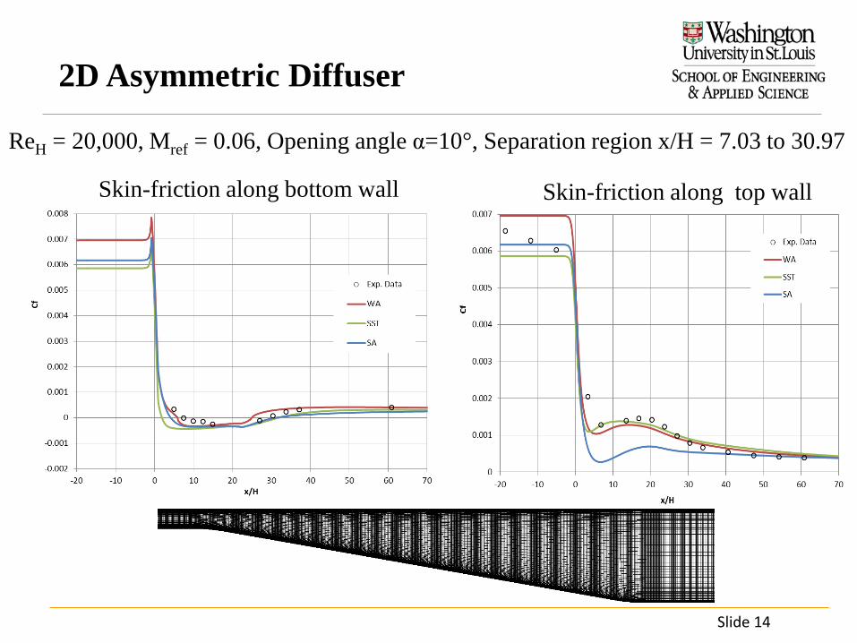
Slide 14
2D Asymmetric Diffuser
ReH = 20,000, Mref = 0.06, Opening angle α=10°, Separation region x/H = 7.03 to 30.97
Skin-friction along bottom wall Skin-friction along top wall

Slide 15
2D Wall-Mounted Hump
-1.0
-0.8
-0.6
-0.4
-0.2
0.0
0.2
0.4-0.5 0.0 0.5 1.0 1.5 2.0
Cp
x/c
exp. Cp
WA-DES
WA
SA
ReC = 936,000, Mref = 0.1, Surface Pressure Coefficient
-1
-0.8
-0.6
-0.4
-0.2
0
0.2
0.4-0.5 0 0.5 1 1.5 2
Cp
x/c
Exp. DataWASST k-ω SA

Slide 16
ReC = 936,000, Mref = 0.1, Surface skin friction coefficient
2D Wall-Mounted Hump
All models reattach in the range of x/c = 1.26-1.29 except WA-DES (x/c = 1.10)
-0.004
-0.002
0.000
0.002
0.004
0.006
0.008
-0.5 0.0 0.5 1.0 1.5 2.0
Cf
x/c
exp. Cf
WA-DES
WA
SA
-0.004
-0.002
0
0.002
0.004
0.006
0.008
-0.5 0 0.5 1 1.5 2
Cf
x/c
Exp. DataWASST k-ω SA
Experiment reattachment at x/c = 1.10±0.03

Slide 17
2D NACA4412 Rec = 1.52x10⁶, Mref = 0.09, α = 13.9°, Separation point varies from x/c = 0.6 to 0.7

Slide 18
2D Axisymmetric Separated Boundary Layer
ReH = 2x10⁶, Mref = 0.08812 Surface pressure coefficient
Surface skin friction coefficient

Periodic Hill • Re =10,595 based on hill height h and bulk velocity Ub at the crest of first hill.
Skin friction coefficient
Cp distribution
Slide 19

NASA Glenn S-Duct • M = 0.6, Re = 2,600,000 at s/D1 = -0.5 (Plane A) • The Aerodynamic Interface Plane (AIP), where the turbine
face is located, is at s/D1 = 5.73 (Plane E)
20

NASA Glenn S-Duct
21
0
0.1
0.2
0.3
0.4
0.5
0.6
0 1 2 3 4 5
Cp
S/D1
Exp. 10Deg
WA-DES
WA
SA
-0.1
0
0.1
0.2
0.3
0.4
0.5
0.6
0 1 2 3 4 5
Cp
S/D1
Exp. 90Deg
WA-DES
WA
SA
-0.3
-0.2
-0.1
0
0.1
0.2
0.3
0.4
0.5
0.6
0.7
0 1 2 3 4 5
Cp
S/D1
Exp. 170Deg
WA-DES
WA
SA

Axisymmetric Transonic Bump
• Freestream Mach number M = 0.875, Reynolds number Rec=2,763,000 • Separation region varies from x/c = 0.7 to 1.1
22
-0.8
-0.7
-0.6
-0.5
-0.4
-0.3
-0.2
-0.1
0.0
0.1
0.20.4 0.6 0.8 1.0 1.2 1.4 1.6
Cp
x/c
Exp. Cp
WA-DES
WA
SA
Experiment WA-DES % Error WA % Error SA % Error
Separation 0.7 0.696 0.571 0.817 16.714 0.688 1.714
Reattachment 1.1 1.106 0.6 1.123 2.091 1.160 5.455

“Run5”, Pnozzle = 31.71 Psia, Tnozzle = 648 R, Mixing Section Throat = 1.25”, �̇�𝑆𝑛𝑛𝑐𝑐𝑧𝑧𝑧𝑧𝑙𝑙𝑒𝑒 = 0.0787
2D Slot Nozzle Ejector

3D Supersonic Flow in a Square Duct Experiment of Davis and Gessner, M = 3.9, ReD= 508,000, D = 25.4mm, x/D = 50

System Rotation and Curvature
Slide 25
• The main characteristic of system rotation and large curvature flows is the additional turbulent production experienced in these flows.
• For this reason, corrections to turbulence models aim to increase the production term or decrease the destruction term in the transport equations.
• The Spalart-Shur correction multiplies the production term by a rotation function 𝑓𝑓𝑟𝑟1 𝑎𝑎∗, �̃�𝑎 = 1 + 𝑐𝑐𝑟𝑟1
2𝑟𝑟∗
1+𝑟𝑟∗1 − 𝑐𝑐𝑟𝑟3 tan−1 𝑐𝑐𝑟𝑟2�̃�𝑎 − 𝑐𝑐𝑟𝑟1, 𝑎𝑎∗= 𝑆𝑆
𝑊𝑊
• Modification of coefficients in Spalart-Shur RC correction using UQ:
• Zhang and Yang RC correction
• Durbin-Arrola correction
Turbulence model 𝐂𝐂𝐫𝐫𝐫𝐫 𝐂𝐂𝐫𝐫𝐫𝐫 𝐂𝐂𝐫𝐫𝐫𝐫
Original WA-RC 1.0 12.0 1.0
Modified WA-RC 1.0 0.1 0.1

Rotation & Curvature Benchmark Cases
Slide 26
• 2D Curved Duct • 2D U-turn Duct • 2D Rotating Channel • 2D Rotating Backward-facing Step • Rotating Cavity – Radial Inflow • Rotating Cavity – Axial Inflow • Serpentine Channel • Rotating Serpentine Channel • Rotor-Stator Cavity • Hydrocyclone • Supersonic Jet in Crossflow

Rotating Serpentine Channel
Slide 27
Geometry and Input The geometry is 12πδ×2δ with a curvature ratio 𝐷𝐷𝑐𝑐/𝛿𝛿 = 2 based on the channel half-width δ. Reynolds number: 𝐷𝐷𝑒𝑒 ≡ 2𝛿𝛿𝑈𝑈𝑏𝑏/𝜈𝜈 = 5600 Rotation number: 𝐷𝐷𝑐𝑐 ≡ 2𝛿𝛿Ω/𝑈𝑈𝑏𝑏 = 0.32

Serpentine Channel
Slide 28
Mean Velocity Profile

Rotating Serpentine Channel
Slide 29
Mean Velocity Profile

WA-Rough
Slide 30
• Follows the procedure of the SA-Rough model.
𝑑𝑑𝑛𝑛𝑒𝑒𝑤𝑤 = 𝑑𝑑 + 0.03𝐷𝐷𝑠𝑠
𝑓𝑓𝜇𝜇 =𝜒𝜒3
𝜒𝜒3 + 𝐶𝐶𝑤𝑤3, 𝜒𝜒 =
𝐷𝐷𝜈𝜈
+ 𝐶𝐶𝑟𝑟1𝐷𝐷𝑠𝑠𝑑𝑑
• Wall boundary condition for R becomes:
𝜕𝜕𝐷𝐷𝜕𝜕𝑚𝑚
=𝐷𝐷
𝑑𝑑𝑛𝑛𝑒𝑒𝑤𝑤
• To further increase the eddy-viscosity near the wall
𝐶𝐶2𝑘𝑘𝜔𝜔 𝑟𝑟 = 𝐶𝐶2𝑘𝑘𝜔𝜔1
1 + 𝐶𝐶𝑟𝑟2𝐷𝐷𝑠𝑠𝑑𝑑𝑛𝑛𝑒𝑒𝑤𝑤

Smooth and Rough S809 Airfoil
Slide 31
NREL’s S809 Airfoil commonly used in HAWT Rec = 1x10⁶ , U = 12.8 m/s, α = 0̊, 2̊, 4̊, 6̊, 8̊, 10̊, 12̊ Roughness pattern was developed using a molded insect pattern taken from a field wind turbine. ks/c= 0.0019

WA-γ Transition Model
Slide 32
𝛾𝛾 = intermittency parameter, 𝑃𝑃𝐷𝐷𝑙𝑙𝑖𝑖𝑆𝑆 ensure proper R generation for very low Tu values 𝐹𝐹𝑐𝑐𝑛𝑛𝑠𝑠𝑒𝑒𝑡𝑡 triggers the intermittency production, it is a function of 𝐷𝐷𝑇𝑇 ,𝐷𝐷𝑒𝑒𝑣𝑣, and 𝐷𝐷𝑒𝑒𝜃𝜃𝑐𝑐
Local TurbulenceIntensity: 𝑇𝑇𝜕𝜕𝐿𝐿 = min 100 2𝑅𝑅3
𝑅𝑅0.3∗𝑑𝑑𝑤𝑤
, 100 ,𝑑𝑑𝑤𝑤~distance from wall
Pressure gradient parameter: λ𝜃𝜃𝐿𝐿 = −7.57 ∙ 10−3 𝑑𝑑𝑑𝑑𝑑𝑑𝜕𝜕
𝑑𝑑𝑤𝑤2
ν+ 0.0128
𝐷𝐷𝑒𝑒𝜃𝜃𝑐𝑐 correlation: 𝐷𝐷𝑒𝑒𝜃𝜃𝑐𝑐 = 100.0 + 1000.0exp [−1.0 ∗ 𝑇𝑇𝜕𝜕𝐿𝐿 ∗ 𝐹𝐹𝑃𝑃𝑃𝑃] where FPG is a correlation function of λ𝜃𝜃𝐿𝐿

WA-γ Transition Model
Slide 33
• Three zero pressure gradient flat plate cases : T3A, T3B, T3A-
𝑼𝑼∞ (m/s) 𝑻𝑻𝑻𝑻∞(%) 𝝁𝝁𝑻𝑻/𝛍𝛍 ρ (kg/m3) μ (kg/ms) Re
T3A 5.4 3.5 13.3 1.2 1.8e-5 9e+5 T3B 9.4 6.5 100 1.2 1.8e-5 1.57e+6
T3A- 19.8 0.874 8.72 1.2 1.8e-5 3.3e+6
-1E+5 1E+5 3E+5 5E+5 7E+50
0.002
0.004
0.006
0.008
0.01
Rex
Cf
-3E+5 2E+5 7E+5 1E+60
0.002
0.004
0.006
0.008
0.01
Rex
Cf
T3A T3B T3A-
-5E+5 5E+5 2E+6 3E+60
0.001
0.002
0.003
0.004
0.005
0.006
Rex C
f
Experiment
SST-Transition
WA-Transition

Summary
Slide 34
• A new one-equation turbulence model has been developed to have desirable characteristics of one-equation k-ω and one equation k-ε models.
• The new one-equation WA model has been used to simulate a number of wide-ranging canonical turbulent flow cases.
• The behavior of the WA model is very similar to the two-equation SST k-ω model.
• A clear advantage of the WA model’s predictive capability over the SA model has been shown for a number of cases from subsonic to transonic to hypersonic wall bounded flows with small regions of separation and subsonic/supersonic free shear layer flows.
• Spalart-Shur R/C correction has been implemented and verified for all three models.
• Surface roughness corrections have been implemented and verified for all three models.
• The DES and IDDES versions of WA model have been developed which show improvement in accuracy over the WA model.

Acknowledgements
Slide 35
• This research has been partially supported by NASA EPSCoR Program.
• PI is very grateful to Dr. Mujeeb Malik for his support and help.
• The presentation is based on the work of many graduate students: Tim Wray, Xu Han, Hakop Nagapetyan, Xiao Zhang, Francis Acquaye, Colin Graham and Isaac Witte
• The research has been presented at AIAA and ASME conferences .
• The conference papers and journal papers are available.
• Code modules for OpenFOAM and Fluent UDFs are available upon request.


