
Distributed and Pointwise Control forParabolic PDE: A Numerical Approach
L. Héctor Juárez V. and Diana A. León
Departamento de Matemáticas–UAM Iztapalapa
International Workshop on Statistical and Computational Methodsfor Inverse Problems

Control Problem
A control problem consists of:
1. An input–output process (controled system).
2. Observations of the output of the controled system.
3. An objective to be achieved.
Interest: Drive the system to a state that satifies a prescribed criteriumor objective. We are interested in systems modeled by PDE.
Input: A function υ ←→ (control variable)
Output: Solution y of the PDE ←→ (state of the system)
Controls y objetives
The control (input) υ can be a function:
I Defined on the boundary.
I Defined in a subdomain.
I The initial condition.
I One of the parameters.
Objetives: we can seek a control υ to:
I Minimize a criterium or cost: optimal control.
I Reach an observable state: controllability problem.
I Stabilize a system or a state: stabilization problem.

Example: cathodic protectionA metal placed in a corrosive electrolyte tends to ionize and dissolve. To prevent corro-sion, another metal (less noble) can be placed in the electorlyte to form an electrochem-ical cell.
In this process the noble metal plays the role of cathode, and the other one the roleof anode. A current i can be prescribed to the anode to modify the electric field in theelecrolyte. This system is described by
−∇ · (σ∇φ) = 0, in Ω,
−σ∂σ
∂n= i on Γa, 0 on ΓN , g(φ) on Γc
g(φ) is the cathodic polarization function (nolinear).

The cathode is protected if the electric potential is close to a givenvalue φ on Γc .
Here, the control is i , the output is φ and the objective is to minimizethe following functional:
J(φ) =
∫Γc
(φ− φ
)2 dΓ
where (φ, i) ∈ H1(Ω)× L2(Γa) y a ≤ i ≤ b.
A compromise between cathodic protection and consumed energy canbe obtained from the minimization of
J(φ) =
∫Γc
(φ− φ
)2 dΓ + α
∫Γa
i2 dΓ.

Example: stabilization of a bending beam
Equations of motion of the Timoshenko beam:
ρ∂2u∂t2 − K
(∂2u∂x2 −
∂φ
∂x
)= 0 in (0,L),
Iρ∂2φ
∂t2 − EI∂2φ
∂x2 + K(φ− ∂u
∂x
)= 0 in (0,L),
u(0, t) = φ(0, t) = 0, t ≥ 0.
I u: deflection of the beam.
I φ: angle of rot. of cross sections.
I ρ: mass density per unit length.
I EI: flexural rigiditey of the beam.
I Iρ: mass moment of inertia.
I K : shear modulus.

If a boundary control force f1 and a control moment f2 is applied atx = L, the boundary conditions are
K [φ(L, t)− ux (L, t) ] = f1(t) for t ≥ 0−EI φx (L, t) = f2(t) for t ≥ 0,
Stabilization problem
Find f1 and f2 so that the energy of the beam
E(t) =12
∫ L
0
ρu2
t (t) + Iρ φ2t (t) + K [φ(t)− ux (t) ]2 + EI φ2
x (t)
dx
decay to zero (asymtoticaly and uniformly).

Example: identification of a pollution source
A model for the dispersion of a pollutant in water is
∂y∂t− ν ∆y + v0 · ∇y = s(t) δa in Ω× (0,T )
∂y∂n
= 0 on Γ× (0,T )
y(x ,0) = y0(x) in Ω
I y(x , t), pollutant concentration.
I ν, water vscosity.
I v0, water velocity.
I s(t), flow rate of pollution.
I a ∈ K , source position, (K ⊂ Ωcompact).

Identification problem
We suppose that the concentration of the pollutant yobs(x , t) can bemeasured in a subset O ∈ Ω in an interval of time [0,T ].
Problem: Find the pollution source a ∈ K that minimizes
J(y) =
∫ T
0
∫O
(y − yobs)2 dx
Related problem: Estimate de flow rate s(t), satisfying a priory boundssl ≤ s(t) ≤ su. This is when the pollution source is known but notaccessible.

Model problem: Parabolic PDE
Let Ω ∈ Rd , Γ = ∂Ω, T > 0
Q = Ω× (0,T ), Σ = Γ× (0,T )
State equation: Given y0 ∈ L2(Ω), findy = y(x , t) such that
∂y∂t
+A y = f in Q,
y = 0 on Σ,
y(0) = y0, in Ω.
Possibilities for Aφ:
−∆φ, −∇ · (A∇φ), −∇ · (A∇φ) + v0 ·∇φ

Properties of operator A
Linear and continous
A : H1(Ω) −→ H−1(Ω)
Elliptic 〈Aφ, φ〉 ≥ α ‖φ‖2H1
0 (Ω).
Selfadjoint 〈Aφ, φ〉 = 〈φ,Aφ〉.
Unique solution: y ∈ L2(0,T ; H1
0 (Ω)),
∂y∂t∈ L2
(0,T ; H−1(Ω)
).
The solution y is continous from [0,T ] to L2(Ω)

Controllability
Controllability problem: Let T > 0 be a finite time, and let yT be atargent function in the state space.
Is it possible to drive the system from a given initial state y0 to a finalprescribed state yT in the given interval of time?.
Distributed control: Given yT ∈ L2(Ω) findυ ∈ L2(O × (0,T )) such that
∂y∂t
+A y = υ χO×(O,T )in Q,
y = 0 on Σ,
y(0) = y0 in Ω,
y(T ) = yT in Ω.
We have taken f = 0 for simplicity.

Exact and approximate controllability
Exact controllability
The system is controlable (or axactly controlable) when there exists acontrol υ for each target yT .
Exact controllability es very strict and it is not always possible. So, inpractice the condition y(T ) = yT is relaxed by the less restricted
Approximate controllability
In this case we look for a control υ that drives the system, in a finitetime T > 0, to a state y(T ; υ) within a small neighboorhood of yT .
More precisely: Let B be the unit ball in L2(Ω), we look for a control υsuch that
y(T ; υ) ∈ yT + εB, for ε small.

Reformulation as an optimal control
The following density result tell us that, for the approximate controla-bility problem, there are infinitely many possible controls.
If υ spans L2(O×(0,T )), then y(T ; υ) spans an affine dense subspacein L2(Ω).
We compute the control with minimal norm:
inf12
∫ T
0
∫Ω
υ2 dx dt , υ ∈ L2(O × (0,T )), y(T ; υ) ∈ yT + εB
This problem has a unique solution. Moreover
I T > 0, can be choosen arbitrarily small.
I O ⊂ Ω, may be choosen arbitrarily small.

Penalization
Alternative: The optimal control problem can be reformulated:
inf Jk (υ) =12
∫ T
0
∫Ω
υ2 dx dt +k2‖y(T ; υ)− yT‖2
L2(Ω) υ ∈ L2(O×(0,T )).
Result: There exists k large enough, such that the minimun uk of Jkverifies:
‖y(T ; uk )− yT‖ ≤ ε (k ∝ 1/ε)
I The solution can be reached by methods acting directly on thecontrol υ.
I We can also apply convex duality theory.

Optimality system
The minimum uk of Jk (υ) satisfies the following optimality system:
∂y∂t
+A y = ψ χO×(O,T )in Q, y(0) = 0, y = 0 sobre Σ
−∂ψ∂t
+A∗ ψ = 0 in Q, ψ(T ) = k (yT − y(T )), ψ = 0 on Σ.
uk = ψ χO×(O,T )
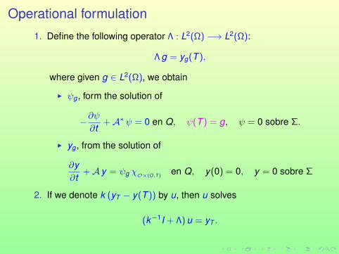
Operational formulation
1. Define the following operator Λ : L2(Ω) −→ L2(Ω):
Λ g = yg(T ),
where given g ∈ L2(Ω), we obtain
I ψg , form the solution of
−∂ψ∂t
+A∗ ψ = 0 en Q, ψ(T ) = g, ψ = 0 sobre Σ.
I yg , from the solution of
∂y∂t
+A y = ψg χO×(O,T )en Q, y(0) = 0, y = 0 sobre Σ
2. If we denote k (yT − y(T )) by u, then u solves
(k−1I + Λ) u = yT .

The operational equation
Lu = yT , with L =(k−1I + Λ
)is the Euler–Lagrange equation of a quadratic minimization problem,
then we can apply a gradient descent method to solve it.
Once u is obtained, the control is found by solving first
−∂ψ∂t
+A∗ ψ = 0 en Q,
ψ(T ) = u, en Ω,
ψ = 0 sobre Σ.
Therefore, the control is uk = ψ χO×(O,T ).

Comjugate gradient algorithm
1. Inicialization: Given u0, compute g0 = Lu0 − yT and d0 = −g0.
2. Descent: Assuming we know uk , gk , dk , find uk+1, gk+1,dk+1
doing the following
uk+1 = uk + αk dk , with αk =〈gk , gk 〉〈dk , Ldk 〉
gk+1 = gk + αk Ldk
Test of convergence: If ‖gk+1‖ ≤ ε‖g0‖, take u∗ = uk+1 andstop. Otherwise, go to step 3.
3. New conjugate direction
dk+1 = −gk+1 + βk dk , with βk =〈gk+1,gk+1〉〈gk , gk 〉
Do k = k + 1 and go to step 2.

Numerical examplesIn all cases we solved the state and adjoint equations by the finiteelement method with ∆x = ∆ t = 0.01.
∂y∂t− ∂2y∂x2 = υ χO×(0, T )
in Q = (0,1)× (0,T ),
y = 0 on Σ = Γ× (0,T )
y(0) =
x , x ≤ 1/2;1− x , x > 1/2.
y(T ) = yT
Example 1. (smooth target) yT = 4x(1− x)
Example 2. (nonsmooth target) yT =
8(x − 14 ), if 1/4 ≤ x ≤ 1/2,
8( 34 − x), if 1/2 ≤ x ≤ 3/4,
0, otherwise.
Example 3. (nonsymmetric target) yT = 4 x (1− x) (x − 1/8)

Example 1. Smooth target
yT = 4x(1− x)
|y(T )−yT ||yT | = 0.03 Evolution of the control υ
I Subdomain: O = (0.4, 0.6).
I Final time: T = 2.
I Tolerance: ε = 10−10

Example 2. Nonsmooth target
|y(T )−yT ||yT | = 0.21 Evolution of the control υ
I Subdomain: O = (0.4, 0.6).
I Final time: T = 2.
I Tolerance: ε = 10−10

Example 3. Nonsymmetric target
|y(T )−yT ||yT | = 0.0012
I Subdomain: O = (0, 1).
I Final time: T = 1.
I Tolerance: ε = 10−10

Pointwise control
Problem: Given yT , find υ and y such that
∂y∂t− µ
∂2y∂x2 = υ(t)δ(x − b) in Q = (0,1)× (0,T ),
y = 0 on Σ = Γ× (0,T ),
y(0) = 0y(T ) = yT
I The state equation has a unique solution for each υ ∈ L2(0,T ).
I For d ≤ 3, y ∈ L2(Q), and ∂y∂t ∈ L2(0,T ; H−2(Ω)).
I t −→ y(t ; υ) is continuous from [0,T ] into H−1(Ω).
I When υ spans L2(0,T ) then y(T ) = y(T ; υ) spans a subspaceof H−1(Ω)

Orthogonal of the closure of y(T ; υ)υ∈L2(0,T )
〈y(T ; υ), f 〉 =
∫ T
0ψ(b, t) υ(t) dt , f ∈ H1
0 (ω).
I 〈·, ·〉 is the duality pairing between H−1(Ω) and H10 (Ω).
I ψ is the solution of the adjoint equation
−∂ψ∂t
+A∗ψ = 0 in Ω, ψ(T ) = f , ψ = 0 on Σ.
I ψ ∈ L2(0,T ; H2(Ω) ∩ H10 (Ω)).
Therefore, f is ortogonal to y(T ; υυ∈L2(0,T ) ⇐⇒ ψ(b, t) = 0
and
y(T ; υ) spans a dense subset of H−1(Ω) when υ spans L2(0,T )⇐⇒b is such that ψ(b, t) = 0 implies ψ = 0.

Strategic points
Let ωj∞j=1 be the eigenfunctions of A = A∗, and λj∞j=1 thecorresponding eigenvalues.
We say that b is an strategic point in Ω if ωj (b) 6= 0 for all j = 1,2, . . ..
Then ψ(b, t) = 0 implies ψ = 0, since
ψ(x ,T ) = f (x) =∑
j
fj ωj (x), for f ∈ H10 (Ω),
ψ(b, t) =∑
j
fj ωj (b) e−λj (T−t) = 0, only if fj = 0 ∀ j .

Optimal controlSuppose b ∈ Ω is an stategic point. We look for the solution of
infυ∈V
J(υ) =12
∫ T
0υ2 dt
with V = υ ∈ L2(0,T ) : y(T ; υ) ∈ yT + β B−1, and yT ∈ H−1(Ω)and B−1 the unit ball in H−1(Ω).
This problem can be solved using duality arguments. However, fromthe practical point of view, it is easier to solve directly the followingpenalized problem
minυ∈L2(0,T )
Jk (υ) =12
∫ T
0υ2 dt +
k2‖y(T ; υ)− yT‖2
−1, k > 0,
where ‖g‖−1 = ‖ϕg‖H10 (Ω) and ϕg solution of
−4ϕg = 0 in Ω, ϕg = 0 in Γ.

Optimality conditionsThe previous problem has a unique solution u ∈ L2(0,T ), characteri-zad by the existence of p ∈ L2(0,T ; H2(Ω)∩H1
0 (Ω))∩C0([0,T ]; H10 (Ω)),
such that u, y ,p satisfies the following optimality system
∂y∂t
+A y = u δ(x − b) in Q, y = 0 on Σ, y(0) = 0,
−∂p∂t
+A∗ y = 0 in Q, p = 0 on Σ, p(T ) = k(−4)−1(yT − y(T ; u)),
u(t) = p(b, t).
This problem, or equivalently the minimization problem, can be solvedby a gradient descent method, since we can compute its derivative(first variation)∫ T
0J ′k (u) υ dt =
∫ T
0(u(t)− p(b, t)) υ(t) dt , ∀ υ ∈ L2(0.T ).
We apply a conjugate gradient algorithm very similar to the one intro-duced before.

Example 1.

Target function
yT =
8(x − 1
4 ), if 14 ≤ x ≤ 1
2 ,
8( 34 − x), if 1
2 ≤ x ≤ 34 ,
0, otherwise.
Parameters
T = 3, ∆x = ∆t = 10−2.
b k N. Iter ||uk (x ,T )||2L||yT−ym(T )||L2(Ω)
||yT ||L2(Ω)√2
3 103 3 34.1939 0.6249104 4 61.7933 0.3942105 6 79.3059 0.2789106 10 114.3000 0.2184108 26 700.2412 0.14151010 103 3.0216×10³ 0.1242
12 103 3 34.2446 0.6193
104 4 61.8262 0.3766105 6 82.3173 0.2251106 8 122.8655 0.1289108 15 194.5858 0.05851010 30 874.9293 0.0340
π6 103 3 34.2239 0.6246
104 4 61.8236 0.3934105 6 80.0432 0.2762106 10 115.5124 0.2178108 25 670.0066 0.14221010 144 2.7191×10³ 0.1235

Example2.

Unsymmetric target
yT =274
x2 (1− x) ,
Same parameters
b k N. Iter ||uk (x ,T )||2L||yT−ym(T )||L2(Ω)
||yT ||L2(Ω)√2
3 105 6 73.8552 0.3859106 11 154.3000 0.3444108 37 1.4870×10³ 0.14361010 105 2.3732×10³ 0.02281012 91 2.4727×10³ 0.01641015 89 2.4743×10³ 0.0164
12 105 6 65.2239 0.3731
106 7 78.0479 0.3572108 14 103.5828 0.35371010 15 128.9864 0.35361012 15 130.0881 0.35361015 15 130.0995 0.3536
π6 105 6 62.9638 0.3455
106 10 98.5060 0.3231108 26 1.3323×10³ 0.15251010 60 2.3923×10³ 0.02671012 61 2.5580×10³ 0.01921015 61 2.5606×10³ 0.0192

Chattering Control
The eigenfunctions associated to operator A = −µ ∂2
∂x2 , with homogeneosDirichlet boundary conditions are:
ωj (x) =sin(jπx)
|| sin(jπx)||L2(Ω). (1)
In order to be able to control de system, the control point b must be an strate-gic point :
sin(jπb) 6= 0 ∀j ∈ N,
that is, b ∈ I.
Computers don’t “know” irrational numbers, and it is necessary to move thecontrol point in order to rebuild the control, avoiding tha anulation of all eigen-functions. For instance, we can move the control point b in an oscillatory way:
c(t) = b + ε sin (2πf t) , b ∈ Q,
with ε > 0, f > 0.
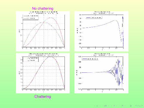
No chattering
Chattering

Target function
yT =274
x2(1− x),
ParametersT = 3, ∆x = ∆t = 10−2,
b = 1/2
ε k N. Iter||yT−ym(T )||L2(Ω)
||yT ||L2(Ω)
0 105 6 0.3731106 7 0.3572108 14 0.35371010 15 0.3536
0.001 105 6 0.3731106 10 0.3551108 37 0.25811010 111 0.0859
0.08 105 10 0.2843106 18 0.1741108 95 0.04661010 530 0.0162
0.1 105 9 0.2669106 20 0.1510108 170 0.0406

No chattering
Chattering

Target function
yT =
8(x − 1
2 ), if 14 ≤ x ≤ 3
4 ,
8(1− x), if 34 ≤ x ≤ 1,
0, otherwise.
Parameters
T = 3, ∆x = ∆t = 10−2, b = 1/2
ε k N. Iter||yT−ym(T )||L2(Ω)
||yT ||L2(Ω)
0 105 6 0.7617106 7 0.7218108 22 0.70941010 29 0.7079
0.001 105 6 0.7627106 10 0.7180108 46 0.49921010 218 0.1397
0.08 105 10 0.5898106 23 0.3135108 136 0.0790
0.1 105 9 0.5488106 20 0.2636108 143 0.0675


