

DPRIETI Discussion Paper Series 15-E-130
Does Exporting Improve Firms' CO2 Emissions Intensity and Energy Intensity? Evidence from Japanese manufacturing
JINJI NaotoRIETI
SAKAMOTO HiroakiChiba University
The Research Institute of Economy, Trade and Industryhttp://www.rieti.go.jp/en/
RIETI Discussion Paper Series 15-E-130
November 2015
Does Exporting Improve Firms' CO2 Emissions Intensity and Energy Intensity? Evidence from Japanese manufacturing*
JINJI Naoto SAKAMOTO Hiroaki
Kyoto University Chiba University
RIETI
Abstract
Using Japanese firm-level data, we investigate the firm-level relationship between export status and
environmental performance in terms of carbon dioxide (CO2) emissions intensity and energy
intensity. As in previous studies, we first find that exporting firms have significantly lower CO2
emissions/energy intensity. We then investigate the effects of exporting on CO2 emissions/energy
intensity by employing the propensity score matching (PSM) method, and find that the effects
significantly vary across industries. Whereas exporting significantly improves environmental
performance in most industries, exporting actually increases CO2 emissions/energy intensity in the
iron & steel industry. This finding suggests that the effect of exporting varies across industries.
Keywords: Trade and the environment, Environmental performance, CO2 emissions, Energy
intensity
JEL classification: F14, F18, Q56
RIETI Discussion Papers Series aims at widely disseminating research results in the form of professional
papers, thereby stimulating lively discussion. The views expressed in the papers are solely those of the
author(s), and neither represent those of the organization to which the author(s) belong(s) nor the Research
Institute of Economy, Trade and Industry.
*This study was conducted as part of the Project “Research on Trade/Foreign Direct Investment and the Environment/Energy” undertaken at the Research Institute of Economy, Trade and Industry (RIETI). We thank Masahisa Fujita, Masayuki Morikawa, Ryuhei Wakasugi, Makoto Yano, and members of the RIETI project for their helpful comments on earlier versions of the paper. We are grateful to the Research and Statistics Department of the Ministry of Economy, Trade and Industry (METI) for granting permission to access firm-level data of the METI’s survey and the Quantitative Analysis and Database Group of RIETI for helping us to apply for the access to the METI’s survey data. We also thank Shuichiro Nishioka for helping us construct clean data for emissions and giving us very detailed comments.

1 Introduction
The issue of trade and the environment has been getting increased attention in eco-
nomics in the last two decades (Copeland and Taylor, 2003, 2004). A number of em-
pirical studies have investigated the environmental effects of trade openness (Antweiler
et al., 2001; Cole and Elliot, 2003; Managi et al., 2009). Antweiler et al. (2001) find
that sulfur dioxide (SO2) concentrations decrease as trade openness rises. Cole and
Elliot (2003) support the finding by Antweiler et al. (2001) for SO2 but do not find
similar results for other pollutants such as nitrogen oxides (NOx) and biochemical
oxygen demand (BOD). Managi et al. (2009) address the endogeneity issue and find a
somewhat mixed result: whereas trade is beneficial to the environment in OECD coun-
tries for SO2, CO2, and BOD, it has detrimental effects on SO2 and CO2 in non-OECD
countries.
Recently, the focus of the research has shifted to the micro-level relationship be-
tween trade and environment. In particular, the firm-level (or plant-level) relation-
ship between export status and the environmental performance has been examined
by several recent studies (Batrakova and Davies, 2012; Cui et al., 2012; Forslid et
al., 2011; Holladay, 2010). Using a panel of firm-level data for Irish manufactur-
ing industries for 1991–2007, Batrakova and Davies (2012) find that export status is
associated with an increase in energy intensity (i.e., total fuel and power purchase
per sales) for low-energy-intensity firms and with a decrease in energy intensity for
high-energy-intensity firms. Holladay (2010) employs a panel of establishment-level
data for US manufacturing industries during 1990–2006 and estimates the export pre-
mium on environmental performance as measured by toxic pollution emissions. He
provides evidence that exporters emit less toxic emissions than non-exporters when
controlling for establishment output and industry characteristics. Moreover, Cui et al.
(2012) use facility-level data of the US manufacturing industry for the years 2002,
2005, and 2008, and analyze the relationship between export status and emissions in-
tensity for air pollutants. They find a significantly negative correlation between export
status and emission intensity. Finally, using Swedish firm-level data for CO2 emis-
sions during 2000–2007, Forslid et al. (2011) test predictions from the model they
develop in which emissions from production are incorporated into a Melitz (2003)
type model. They find that exporters have, on average, lower emissions intensity than
non-exporters.
In this paper, we examine the firm-level relationship between export status and
2
environmental performance in terms of CO2 emissions intensity and energy inten-
sity, using Japanese manufacturing data. We address two important issues, which
have rarely been examined by previous studies. First, we estimate whether exporting
increases or decreases CO2 emissions/energy intensity by employing the propensity
score matching (PSM) method developed by Rubin (1974) and Rosenbaum and Ru-
bin (1983). Second, we pay attention to sectoral variations in the relationship between
exporting and CO2 emissions/energy intensity. Previous studies (Forslid et al., 2011;
Cui et al., 2012) assume that the same mechanism can be applied to all manufactur-
ing industries. However, the effects of exporting on environmental performance may
depend on production technique, product composition, or industrial structure.
To examine the above issues, we employ Japanese firm-level data from two data
sources for the period 2006–2011. The first data source is Mandatory Greenhouse
Gas Accounting and Reporting System, which is provided jointly by the Ministry of
Economy, Trade, and Industry (METI) and the Ministry of Environment (MOE). This
data set includes plant-level emission data for major greenhouse gases (GHGs). The
second data source is the Basic Survey of Japanese Business Structure and Activi-
ties, which is an annual survey conducted by METI. This survey data contain various
firm-level information including export values. We aggregate the plant-level GHG
data to firm-level data, and match the two data sets mentioned above. As for our
empirical strategy, we first estimate the firm-level relationship between exporting and
CO2 emissions/energy intensity by ordinary least square (OLS), and then estimate the
causal effects of exporting on CO2 emissions/energy intensity by PSM method.
The main findings in this paper are as follows. First, we find from the OLS re-
gressions that exporting firms have significantly lower CO2 emissions/energy intensity
than non-exporting firms. This finding is consistent with those in previous studies (Cui
et al., 2012; Forslid et al., 2011; Holladay, 2010). Second, from the PSM analysis, we
find that the effects of exporting on CO2 emissions/energy intensity significantly vary
across industries. In most industries, we find that exporting significantly reduces CO2
emissions/energy intensity, though the magnitude of the effects substantially varies
with industries. For some industries, however, such as paper and metal products, the
effects are statistically insignificant. Surprisingly, there is an industry, namely the iron
and steel industry, in which exporting actuallyincreasesCO2 emissions/energy in-
tensity. We suspect a change in product composition upon exporting may affect CO2
emissions and energy intensity in the iron and steel industry.
Our findings have important policy implications. In the literature on trade and
3

the environment, it has been well known that the environmental effect of trade lib-
eralization can be decomposed into three effects:scale, composition, andtechnique
(Grossman and Krueger, 1993; Copeland and Taylor, 1994). (1) Trade increases real
income, or the economy’s scale, which in turn increases total emissions; this is the
scale effect. (2) Trade also induces countries to specialize in industries in which they
have a comparative advantage, and the consequent changes in the shares of dirtier and
cleaner industries affects total emissions; this is the composition effect. (3) Finally,
if the environment is a “normal good,” an increase in real income increases the de-
mand for the environment and hence the demand for more stringent environmental
regulation, which in turn reduces the emissions intensity of production; this reduction
in emissions intensity is called the technique effect. Whereas the technique effect is a
key for trade to be good for the environment, how the technique effect works has not
been investigated much. The findings of this study reveal one possible mechanism of
the technique effect: we confirm that, on average, firms reduce CO2 emissions/energy
intensity when they start exporting, and that this mechanism does not actually require
any change in environmental regulation. Thus, our findings suggest that the trade-
induced technique effect may work in favor of the environment without any change
in the economy-wide environmental policy. However, we found that the environmen-
tal effects of exporting significantly vary across industries. Therefore, some policy
measures should be implemented to deal with the heterogeneity in the effects across
industries.
The remainder of the paper is organized as follows. Section 2 discusses the theo-
retical background of our empirical analysis. Section 3 explains our data and reports
the results of our preliminary analysis. In section 4, we explain our empirical strategy
to analyze the effects of exporting on environmental performance. Section 5 reports
our empirical results from the PSM analysis. Section 6 discusses our results, and
section 7 concludes.
2 Theoretical Background
In this section, we briefly explain theoretical the background of our empirical analysis.
We do not construct a new model here but instead explain the essence of the models
developed by previous related studies.
The issue is whether there is any systematic relationship at the firm-level between
export status and environmental performance. Cui et al. (2012) present a model of
4

heterogeneous firms based on Melitz (2003). They focus on a single monopolisti-
cally competitive industry, and in their model, technology adoption is a key factor to
determining the relationship between export status and environmental performance.
Pollution is generated as a byproduct of output. The government regulates emissions
by implementing a domestic emission permit cap-and-trade program. Thus, expendi-
ture on emission permits is part of the firms’ variable production costs. Two types of
production technologies are available: clean and dirty. The adoption of clean tech-
nology requires extra fixed costs but reduces marginal costs by decreasing emissions
per unit of output. Moreover, as in Melitz (2003), exporting requires additional fixed
costs and iceberg trade costs. Then, firms decide whether to stay in the market, which
technology to adopt, and whether to export to the foreign market. As in Melitz (2003),
only the most productive firms have an incentive to engage in exporting. In addition,
more productive firms have a higher incentive to adopt the clean technology because
those firms benefit more from reducing marginal costs. Cui et al. (2012) impose cer-
tain assumptions on the parameters and cost structure so that all firms that choose to
adopt the clean technology choose to export and that some of the firms choosing the
dirty technology too export.
Batrakova and Davies (2012) present a model with a similar structure, but include
energy as a production factor, instead of emissions. In their model, technology choice
is associated with the effectiveness of energy usage. That is, a higher technology
increases the energy efficiency of production. Firms differ in both productivity and
energy intensity in production. Then, they show that more productive firms are more
likely to export and also more likely to adopt the energy-efficient technology.
Forslid et al. (2011) consider investment in pollution abatement. Emission taxes
are imposed by the government. Firms can reduce their emissions intensity by two
types of abatement activities. The first type of abatement involves the share of labor
devoted to abatement activities, which incurs variable abatement costs. The second
type of abatement is attained by investments in machines and equipment, which re-
quire fixed costs. Firms optimally choose the fraction of labor devoted to abatement.
Then, Forslid et al. (2011) show that for any given level of productivity, exporters in-
vest more in abatement than non-exporters and hence exporters have lower emissions
intensity than non-exporters.
Barrows and Ollivier (2014) argue that in addition to technology upgradation,
measured emissions intensity may change through changes in prices or product-mix.
This is mainly because emissions intensity is usually measured in value due to data
5
limitations. If exporters and non-exporters charge different prices, then the differ-
ence in emissions intensity between exporters and non-exporters may simply reflect
the price differential without any difference in emissions per output. Similarly, if ex-
porters and non-exporters have a different product-mix, then their average emissions
intensity will differ even though they use the same technology. Therefore, caution is
needed to interpret the empirical finding of lower emissions intensity for exporters.
The view of technology upgrading upon exporting may be misleading. We take this
possibility into account in our empirical analysis.
3 Data and preliminary analysis
To investigate the relationship between exporting and environmental performance, we
combine the two data sets available to analyze the Japanese manufacturing sector.
The first is the Mandatory Greenhouse Gas Accounting and Reporting System pro-
vided jointly by METI and MOE, or the MOE survey. Under the Act on Promotion
of Global Warming Countermeasures, major emitters of GHGs are obliged to report
the amounts of GHG emissions to the government. Firms that use more than 1,500
kl/year of oil equivalent energy or emit more than 3,000 t/year of CO2 equivalent
have to file their details. Contained in the MOE survey is plant-level emission data
for every major GHG. The second data set is the Basic Survey of Japanese Business
Structure and Activities provided by METI, which we hereafter refer to as the METI
survey. This is a mandatory annual survey for all firms with 50 or more employees
and paid-up capital or investment funds exceeding 30 million yen. The METI survey
covers mining, manufacturing, wholesale/retail trade, and service industries, and ap-
proximately 32,000 firms responded to the survey in 2012. In this study, we use data
for only the manufacturing industries. The METI survey contains firm-level informa-
tion for a number of important variables, including sales, employment, capital stock,
and exporting.
For each plant appearing in the MOE survey, we search for the associated firm
registered in the METI survey and match them if any. This matching procedure, con-
ducted over the period of 2006–2011, leaves us with a six-year balanced panel of
1,740 firms.1
Table 1 presents the number of exporting firms and non-exporting firms in each
1The procedure we have employed inevitably restricts our analysis to the balanced panel becauseotherwise one firm would be associated with different number of plants in different points in time.
6
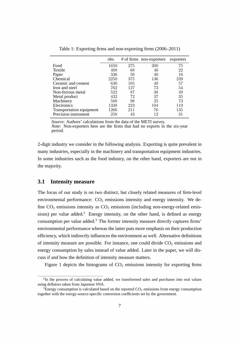
Table 1: Exporting firms and non-exporting firms (2006–2011)
obs. # of firms non-exporters exporters
Food 1650 275 200 75Textile 408 68 46 22Paper 336 56 40 16Chemical 2250 375 136 239Ceramic and cement 630 105 48 57Iron and steel 762 127 73 54Non-ferrous metal 522 87 38 49Metal product 432 72 37 35Machinery 588 98 25 73Electronics 1338 223 104 119Transportation equipment 1266 211 76 135Precision instrument 258 43 12 31
Source: Authors’ calculations from the data of the METI survey.Note: Non-exporters here are the firms that had no exports in the six-yearperiod.
2-digit industry we consider in the following analysis. Exporting is quite prevalent in
many industries, especially in the machinery and transportation equipment industries.
In some industries such as the food industry, on the other hand, exporters are not in
the majority.
3.1 Intensity measure
The focus of our study is on two distinct, but closely related measures of firm-level
environmental performance: CO2 emissions intensity and energy intensity. We de-
fine CO2 emissions intensity as CO2 emissions (including non-energy-related emis-
sions) per value added.2 Energy intensity, on the other hand, is defined as energy
consumption per value added.3 The former intensity measure directly captures firms’
environmental performance whereas the latter puts more emphasis on their production
efficiency, which indirectly influences the environment as well. Alternative definitions
of intensity measure are possible. For instance, one could divide CO2 emissions and
energy consumption by sales instead of value added. Later in the paper, we will dis-
cuss if and how the definition of intensity measure matters.
Figure 1 depicts the histograms of CO2 emissions intensity for exporting firms
2In the process of calculating value added, we transformed sales and purchases into real valuesusing deflators taken from Japanese SNA.
3Energy consumption is calculated based on the reported CO2 emissions from energy consumptiontogether with the energy-source-specific conversion coefficients set by the government.
7

0 2 4 6 8 10
CO2 emission intensity
0.00
0.02
0.04
0.06
0.08
0.10
0.12
0.14
0.16re
lati
ve
freq
uen
cyall industries combined
non-exporters
exporters
Figure 1: Exporters vs. non-exporters
Source: Authors’ calculations from the data of the MOEand METI surveys.
and non-exporting ones observed during the entire sample period. Obviously, the two
groups have different distributions.4 The distribution for exporters is more concen-
trated in the low levels of CO2 emissions intensity. The distribution for non-exporters,
on the other hand, has a fatter tail in the high levels of CO2 emissions intensity. Fig-
ure 2 compares the two groups by year. From this figure, it should be easy to see that
exporting firms are relatively less CO2 emission intensive and that this fact is stable
over time. Hence, similar to the empirical evidence provided by Forslid et al. (2011)
for the Swedish manufacturing sector, our data set of Japanese manufacturing indi-
cates that exporters are, on average, consistently cleaner.5 In general, however, more
productive firms are likely to show higher environmental performance, and at the same
time, have a better chance of starting exports. Therefore, the observed correlation be-
tween exporting and high environmental performance might be a logical consequence
of self-selection. The question of interest then is if and to what extent the apparent
4In fact, the Kolmogorov–Smirnov test result shows that the distribution for exporters is located tothe left of that for non-exporters.
5Although an explicit carbon tax is absent in the Japanese market, energy price in effect works asan implicit tax for CO2 emissions since CO2 emissions is closely connected to energy consumption.
8

2006 2007 2008 2009 2010 20110
2
4
6
8
10
12
14
CO
2em
issi
on
inte
nsi
ty
all industries combined
non-exporters
exporters
Figure 2: Comparison over time
Source: Authors’ calculations from the data of the MOEand METI surveys.
high performance of exporters is actually attributed to exporting.
Another important fact we can see in our data set is that there exists large industry-
level heterogeneity. Table 2 provides the industry-level descriptive statistics on CO2
emissions intensity in our data set. As the table shows, average CO2 emissions in-
tensity significantly varies across different industries. Some industries such as the
ceramic and cement industry are highly CO2 intensive while others such as the trans-
portation equipment industry are not really so. As expected from the preceding dis-
cussion, exporting firms are, on average, cleaner in many industries. In the iron and
steel industry, however, exporters are relatively more CO2 emissions intensive. This
already suggests that aggregation over industries may omit some important aspects
of the trade–environment interplay. Further, it can be seen from the table that the
distributions too are quite heterogeneous. In the chemical industry, for instance, non-
exporters have very diverse emissions intensity values whereas the distribution for ex-
porters is much more concentrated. The opposite is true for the textile industry, where
the distribution for non-exporters has relatively small variance. A similar observation
can be made if we use energy intensity instead of CO2 emissions intensity. With this
industry-level heterogeneity in mind, we separately analyze the effect of exporting on
9

Table 2: CO2 emissions intensity by industry (2006–2011)
mean standard deviation
non-exporters exporters non-exporters exporters
Food 3.70 1.78 12.35 2.43Textile 8.02 4.81 8.73 23.51Paper 10.93 7.30 12.05 10.75Chemical 35.62 4.53 265.52 9.48Ceramic and cement 38.79 13.31 71.05 52.22Iron and steel 6.94 8.62 8.27 15.15Non-ferrous metal 16.28 7.86 49.88 47.10Metal product 3.96 2.31 6.95 3.73Machinery 4.87 1.02 13.94 0.92Electronics 3.90 1.77 7.40 3.06Transportation equipment 2.55 1.60 3.16 2.12Precision instrument 3.48 1.07 5.61 1.34
Source: Authors’ calculations from the data of the MOE and METI surveys.
CO2 emissions/energy intensity for each industry.
3.2 Preliminary analysis
As background for the analysis we conduct later in this paper, we first perform a pre-
liminary analysis on the firm-level relationship between exporting and environmental
performance. Letting INTENSi,t be the intensity measure of firmi at yeart, we run
the following OLS regression:
ln INTENSi,t = α + βEXPORTERi,t + γxi,t + εi,t, (1)
where EXPORTERi,t is an export dummy which is equal to one when firmi is ex-
porting at yeart. Covariatesxi,t contain other relevant characteristics such as pro-
ductivity measured by total factor productivity (TFPi,t), firm size measured by labor
(LABORi,t), and R&D intensity measured by labor share of R&D division within each
firm (RDINTi,t). Our productivity estimates are obtained from the method developed
by De Loecker and Warzynski (2013).6 We also control for industry and year effects.
Our primary interest lies in coefficientβ, which tells us whether exporting firms and
non-exporting ones have significantly different environmental performance. Table 3
and Table 4 show the estimation results for (1) for four different specifications of the
model.
6See Appendix A.1 for more details.
10

Table 3: OLS on log CO2 emissions intensity (all industries combined)
(1) (2) (3) (4)
EXPORTER −0.303∗∗∗ −0.280∗∗∗
(0.025) (0.027)EXPSHARE −0.646∗∗∗ −0.027
(0.093) (0.101)ln TFP −0.309∗∗∗ −0.303∗∗∗
(0.014) (0.014)ln LABOR −0.374∗∗∗ −0.399∗∗∗ −0.409∗∗∗ −0.374∗∗∗
(0.013) (0.013) (0.013) (0.013)RDINT −0.410∗∗∗ −0.441∗∗∗ −0.445∗∗∗ −0.379∗∗∗
(0.050) (0.050) (0.048) (0.048)YEAR yes yes yes yesIND yes yes yes yesObservation 7662 7662 7662 7662R squared 0.442 0.434 0.465 0.474
Note: The values in parentheses are standard errors. Observations with miss-ing values are dropped.∗p < 0.10, ∗∗p < 0.05, ∗∗∗p < 0.01.
It is clear from the tables that exporters do differ from non-exporters. To be more
precise, there is a significant negative correlation between exporting and intensity
measure. Column 1 of Table 3, for example, shows that exporters have on average
30% lower CO2 emissions intensity. This estimate is statistically significant at 1%
level. One might argue that this reflects the effect of the intensive margin, that is,
change in the share of exports in sales (EXPSHAREi,t). Column 2 of the table sug-
gests this possibility because a larger export share apparently implies a lower emis-
sions intensity. As column 4 of the table reports, however, the influence of export
share becomes very small and statistically insignificant once export status and export
share are simultaneously taken into account. Hence, the observed negative correlation
between exporting and emissions intensity is likely to be the effect of the extensive
margin, that is, from becoming an exporter. Further, it is worth mentioning here that
productivity and emissions intensity are negatively correlated. We find in column 3 of
Table 3 that a 1% increase in total factor productivity lowers emissions intensity by
30%. This correlation remains unaffected even after relevant covariates are controlled
for.
The fact that exporters are significantly cleaner than non-exporters does not nec-
essarily imply a causal effect of exporting on CO2 emissions/energy intensity. As
11
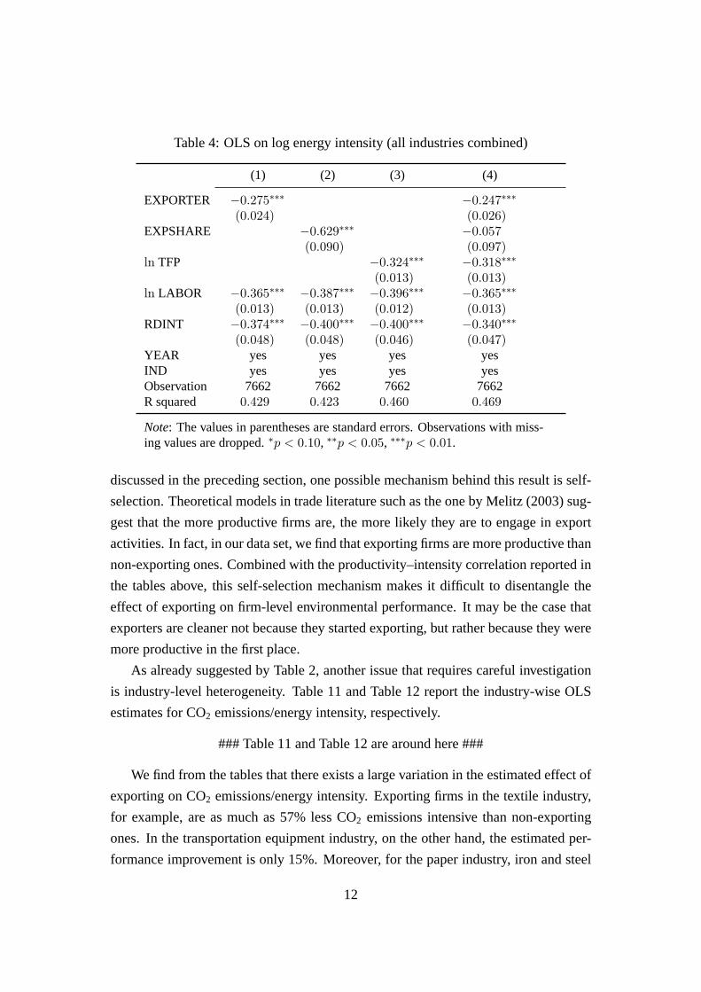
Table 4: OLS on log energy intensity (all industries combined)
(1) (2) (3) (4)
EXPORTER −0.275∗∗∗ −0.247∗∗∗
(0.024) (0.026)EXPSHARE −0.629∗∗∗ −0.057
(0.090) (0.097)ln TFP −0.324∗∗∗ −0.318∗∗∗
(0.013) (0.013)ln LABOR −0.365∗∗∗ −0.387∗∗∗ −0.396∗∗∗ −0.365∗∗∗
(0.013) (0.013) (0.012) (0.013)RDINT −0.374∗∗∗ −0.400∗∗∗ −0.400∗∗∗ −0.340∗∗∗
(0.048) (0.048) (0.046) (0.047)YEAR yes yes yes yesIND yes yes yes yesObservation 7662 7662 7662 7662R squared 0.429 0.423 0.460 0.469
Note: The values in parentheses are standard errors. Observations with miss-ing values are dropped.∗p < 0.10, ∗∗p < 0.05, ∗∗∗p < 0.01.
discussed in the preceding section, one possible mechanism behind this result is self-
selection. Theoretical models in trade literature such as the one by Melitz (2003) sug-
gest that the more productive firms are, the more likely they are to engage in export
activities. In fact, in our data set, we find that exporting firms are more productive than
non-exporting ones. Combined with the productivity–intensity correlation reported in
the tables above, this self-selection mechanism makes it difficult to disentangle the
effect of exporting on firm-level environmental performance. It may be the case that
exporters are cleaner not because they started exporting, but rather because they were
more productive in the first place.
As already suggested by Table 2, another issue that requires careful investigation
is industry-level heterogeneity. Table 11 and Table 12 report the industry-wise OLS
estimates for CO2 emissions/energy intensity, respectively.
### Table 11 and Table 12 are around here ###
We find from the tables that there exists a large variation in the estimated effect of
exporting on CO2 emissions/energy intensity. Exporting firms in the textile industry,
for example, are as much as 57% less CO2 emissions intensive than non-exporting
ones. In the transportation equipment industry, on the other hand, the estimated per-
formance improvement is only 15%. Moreover, for the paper industry, iron and steel
12
industry, and precision instruments industry, the correlation between exporting and
environmental performance becomes statistically insignificant once the other covari-
ates are controlled for. The correlation is even positive in the metal products industry,
although it is not statistically significant. Comparing Table 11 and Table 12, we also
notice that the effect of exporting in the ceramic and cement industry is evident for
CO2 emissions intensity, but not statistically significant for energy intensity. Although
these estimates might be confounded by the well-known correlation between export
status and productivity, our preliminary analysis suggests that the effects of the deci-
sion to start exporting depend on industry.
To examine if the observed differences between exporters and non-exporters are
actually attributed to exporting, and how the effects of exporting on CO2 emissions/energy
intensity differ across industries, we need a counterfactual scenario in which the ex-
porting firms did not start exporting. If we could find a counterfactual substitute for
each exporting firm, we would be able to identify, at least on average, the effects
of exporting by comparing exporters and their counterfactual counterparts. For this
purpose, the present paper employs the matching technique discussed below.
4 Empirical strategy
The econometric method we use in this paper is the propensity score matching (PSM)
method developed by Rubin (1974) and Rosenbaum and Rubin (1983). In essence,
PSM reduces the dimensionality problem in matching firms with multidimensional
characteristics. By constructing a single-dimensional criterion called the propensity
score, it allows us to match an exporter (treated) with a non-exporter (control) based
on the proximity of the score.
4.1 Propensity score
The propensity score is the probability of firms switching from remaining a non-
exporter to becoming an exporter conditional on relevant firm characteristics. To
compute the propensity score for each firm at each point in time, we first specify
the propensity score function as
Pr(STARTi,t = 1 |xi,t−1) = Φ(γxi,t−1), (2)
13

Table 5: Estimated propensity score function
(1) (2) (3)
lnLABOR 0.13553∗∗ 0.95820∗∗ 0.91274∗∗
(0.05400) (0.46391) (0.46322)(lnLABOR)2 −0.06891∗ −0.06429∗
(0.03811) (0.03809)RDINT 0.60381∗∗∗ 1.59904∗∗ 1.60104∗∗
(0.20233) (0.63730) (0.63751)(RDINT)2 −1.87967∗ −1.89118∗
(1.07815) (1.07894)lnTFP 0.01358 −0.23375∗ −0.22347
(0.07660) (0.13841) (0.13884)(lnTFP)2 0.02539∗∗ 0.02409∗∗
(0.01213) (0.01218)FDI 0.58750∗∗∗ 0.59822∗∗∗ 0.59581∗∗∗
(0.11583) (0.11618) (0.11631)CAPINT −0.00131
(0.00159)lnAGE −0.03333
(0.07067)YEAR yes yes yesIND yes yes yesLOCATION yes yes yesObservation 4105 4105 4105AIC 1281 1275 1277Pseudo R squared 0.159 0.169 0.170
Note: The values in parentheses are standard errors.∗p < 0.10, ∗∗p < 0.05,∗∗∗p < 0.01.
whereΦ is the normal cumulative distribution function. Here, STARTi,t is an export-
starting dummy that is1 if firm i starts exporting at periodt. In our data set, there are
151 firms that started exporting during the period 2006–2011. Combining these with
those firms that did not export at any point in the same sample period, we estimated
(2) where covariatesxi,t include a foreign direct investment dummy (FDIi,t), capital–
labor ratio (CAPINTi,t), and firm age (AGEi,t), as well as LABORi,t, RDINTi,t, and
TFPi,t. Firm location is controlled for. The results are presented in Table 5.
As expected, firm size (LABORi,t) and R&D intensity (RDINTi,t) have consis-
tently large impacts on the decision to start exporting. Larger firms that actively invest
in R&D are more likely to switch from remaining a non-exporter to becoming an ex-
porter. In all three specifications, a higher productivity (TFPi,t) positively influences
14

the propensity score although it is not statistically significant for the linear specifica-
tion. While the insignificant coefficient of productivity is not entirely consistent with
the prediction of theoretical models in the literature, our estimation result is largely
in line with the existing empirical studies. Tanaka (2013), for instance, uses the same
METI survey (for a different sample period) and reports a similar finding for the entire
manufacturing sector. Further, Table 5 indicates that the FDI dummy plays an impor-
tant role as well. The experience of foreign direct investment therefore facilitates the
decision to export. Out of the three models listed in the table, we use model 2 for the
analysis that follows.
4.2 Matching
The estimated propensity score function yields the propensity scorePi,t = Φ(γxi,t)
of firm i at yeart. For each exporting firm, we then search for a single non-exporting
counterpart based on the nearest-neighbor matching method with replacement. Denote
by Ji the set of all non-exporters categorized in the same industry as exporteri and
by T the set of years contained in the sample period. Non-exporterji,t ∈ Ji at year
si,t ∈ T is matched with exporteri at yeart if
|Pi,t − Pji,t,si,t | = min(k,τ)∈Ji×T
|Pi,t − Pk,τ | = ∆Pi,t. (3)
Alternatively, one could use different matching algorithms such as radius matching
or kernel matching. The radius matching algorithm is a variant of nearest-neighbor
matching, which considers each match as successful only when the minimum distance
∆Pi,t is smaller than a predetermined radius. Kernel matching, on the other hand, uses
the distance to construct a weight for each non-exporter and employs the weighted
average of non-exporters as a counterfactual of each exporter. We now discuss how
sensitive the estimated causal effects are to the choice of the matching algorithm.
Once we have assembled appropriate exporter and non-exporter pairs, it is straight-
forward to estimate the effect of exporting. What we are interested in here is the av-
erage effect of the treatment on the treated (ATT). Conceptually, ATT compares the
average CO2 emissions/energy intensity among exporters with what the average would
have been had these same firms remained non-exporters. To this end, we substitute the
matched non-exporter for each exporter’s unobservable counterfactual. The estimate
15

Table 6: Effects of exporting on CO2 emissions intensity
ATT t-value % change # matched
Food −1.11∗∗∗ −2.81 −42.5 199Textile −1.67∗∗∗ −3.71 −38.7 65Paper −6.69∗∗∗ −3.06 −54.5 59Chemical −8.95∗∗ −1.98 −69.8 716Ceramic & cement −18.60∗∗∗ −4.86 −73.0 163Iron & steel 2.35∗∗∗ 3.29 48.0 179Non-ferrous metal −4.92∗∗∗ −3.69 −58.8 159Metal product −0.25 −0.59 −9.4 124Machinery −1.22∗∗∗ −6.04 −49.6 234Electronics −2.74∗∗∗ −6.32 −62.7 341Transportation equipment −0.63∗∗∗ −3.68 −27.7 430Precision instrument −3.06∗∗∗ −4.48 −73.8 90All industries combined −4.47∗∗∗ −3.71 −59.2 2759
Note: ∗p < 0.10, ∗∗p < 0.05, ∗∗∗p < 0.01
of the ATT is accordingly calculated as
ATT =
∑i,t(INTENSi,t − INTENSji,t,si,t)
N, (4)
whereN is the number of successfully matched pairs. To shed light on industry-level
heterogeneity, we separately estimate the ATT for each industry.
5 Results
This section reports the effects of exporting on CO2 emissions/energy intensity. We
first present the benchmark results and compare them with the OLS estimates. The
robustness of our findings is then briefly discussed by analyzing the sensitivity to the
matching algorithm and intensity measure.
5.1 Benchmark estimates
Our main results are summarized in Table 6 and Table 7. First, considering all indus-
tries, a considerable improvement is observed in the environmental performance of
exporters. The last row of Table 6 shows that exporting firms achieve a 59% reduction
in CO2 emissions intensity. Similarly, the last row of Table 7 shows that firms become
16
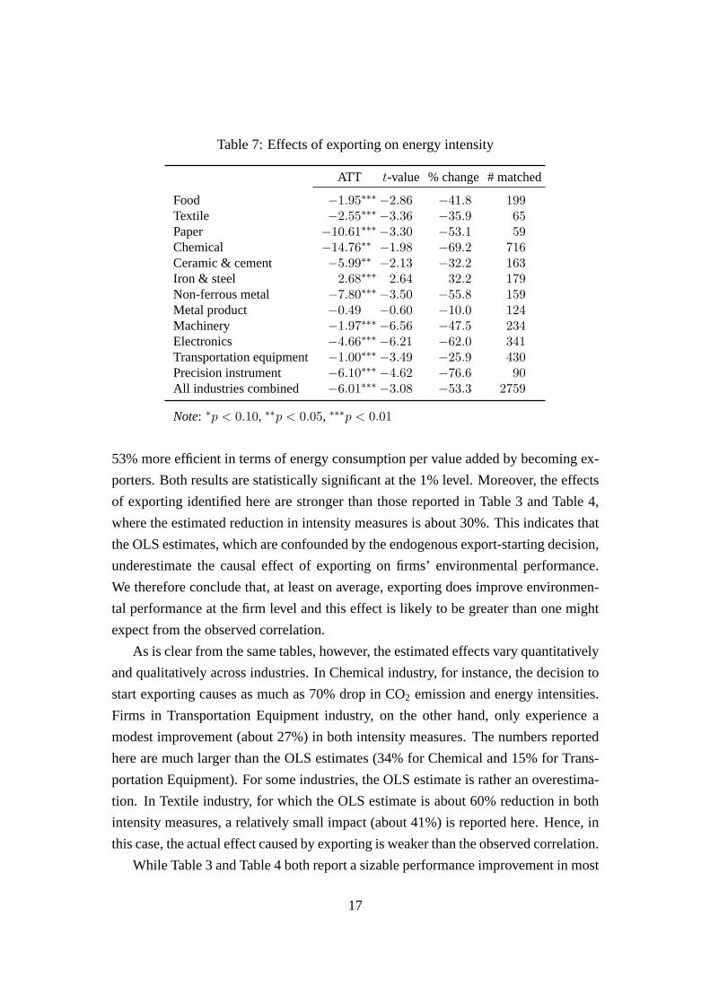
Table 7: Effects of exporting on energy intensity
ATT t-value % change # matched
Food −1.95∗∗∗ −2.86 −41.8 199Textile −2.55∗∗∗ −3.36 −35.9 65Paper −10.61∗∗∗ −3.30 −53.1 59Chemical −14.76∗∗ −1.98 −69.2 716Ceramic & cement −5.99∗∗ −2.13 −32.2 163Iron & steel 2.68∗∗∗ 2.64 32.2 179Non-ferrous metal −7.80∗∗∗ −3.50 −55.8 159Metal product −0.49 −0.60 −10.0 124Machinery −1.97∗∗∗ −6.56 −47.5 234Electronics −4.66∗∗∗ −6.21 −62.0 341Transportation equipment −1.00∗∗∗ −3.49 −25.9 430Precision instrument −6.10∗∗∗ −4.62 −76.6 90All industries combined −6.01∗∗∗ −3.08 −53.3 2759
Note: ∗p < 0.10, ∗∗p < 0.05, ∗∗∗p < 0.01
53% more efficient in terms of energy consumption per value added by becoming ex-
porters. Both results are statistically significant at the 1% level. Moreover, the effects
of exporting identified here are stronger than those reported in Table 3 and Table 4,
where the estimated reduction in intensity measures is about 30%. This indicates that
the OLS estimates, which are confounded by the endogenous export-starting decision,
underestimate the causal effect of exporting on firms’ environmental performance.
We therefore conclude that, at least on average, exporting does improve environmen-
tal performance at the firm level and this effect is likely to be greater than one might
expect from the observed correlation.
As is clear from the same tables, however, the estimated effects vary quantitatively
and qualitatively across industries. In Chemical industry, for instance, the decision to
start exporting causes as much as 70% drop in CO2 emission and energy intensities.
Firms in Transportation Equipment industry, on the other hand, only experience a
modest improvement (about 27%) in both intensity measures. The numbers reported
here are much larger than the OLS estimates (34% for Chemical and 15% for Trans-
portation Equipment). For some industries, the OLS estimate is rather an overestima-
tion. In Textile industry, for which the OLS estimate is about 60% reduction in both
intensity measures, a relatively small impact (about 41%) is reported here. Hence, in
this case, the actual effect caused by exporting is weaker than the observed correlation.
While Table 3 and Table 4 both report a sizable performance improvement in most
17

industries, there are two notable exceptions. First, for the metal products industry,
we find no statistically significant effect of exporting on CO2 emissions/energy inten-
sity. Although consistent with the associated OLS estimate, this finding is remarkable
since exporting firms in this industry are cleaner than non-exporting ones on aver-
age (Table 2). This, therefore, indicates that at least for the metal products industry,
the self-selection mechanism completely explains the observed higher environmental
performance of exporters. Second, somewhat surprisingly, firms in the iron and steel
industry experience a 48% increase in CO2 emissions intensity from exporting. This
counterintuitive result is statistically significant at the 1% level, exhibiting a striking
contrast to our preliminary analysis, where the OLS regression suggests the opposite.
Moreover, a closer inspection of Table 6 and Table 7 reveals that for some in-
dustries, the effects of exporting are substantially different in CO2 emissions/energy
intensity. The estimated improvement of firm-level environmental performance in the
ceramic and cement industry, for example, is much larger for CO2 emissions intensity
(73%) than for energy intensity (32%). This suggests that for exporting firms in this
industry, a sizable portion of the environmental gain materializes as a reduction in non-
energy-related CO2 emission per value added. Similarly, the performance-worsening
effect in the iron and steel industry is much less pronounced (32%) and is statistically
less significant when the intensity is measured by energy consumption instead of CO2
emissions. This is an indication that a major part of the additional CO2 emissions
resulting from exporting in this industry is not energy-related.
5.2 Robustness
Before further discussions on the implications of our findings, let us check if the main
results are sufficiently robust. In particular, we verify to what extent the results depend
on the matching algorithm and the definition of intensity measure.
5.2.1 Alternative matching algorithms
The benchmark estimates presented above are obtained based on the nearest-neighbor
matching method. As a robustness check, we also used radius matching and kernel
matching and computed the associated ATT estimates.7 The first three columns of
7For radius matching, we set the radius to0.01. For kernel matching, we use the Gaussian kernelwith bandwidth0.001.
18
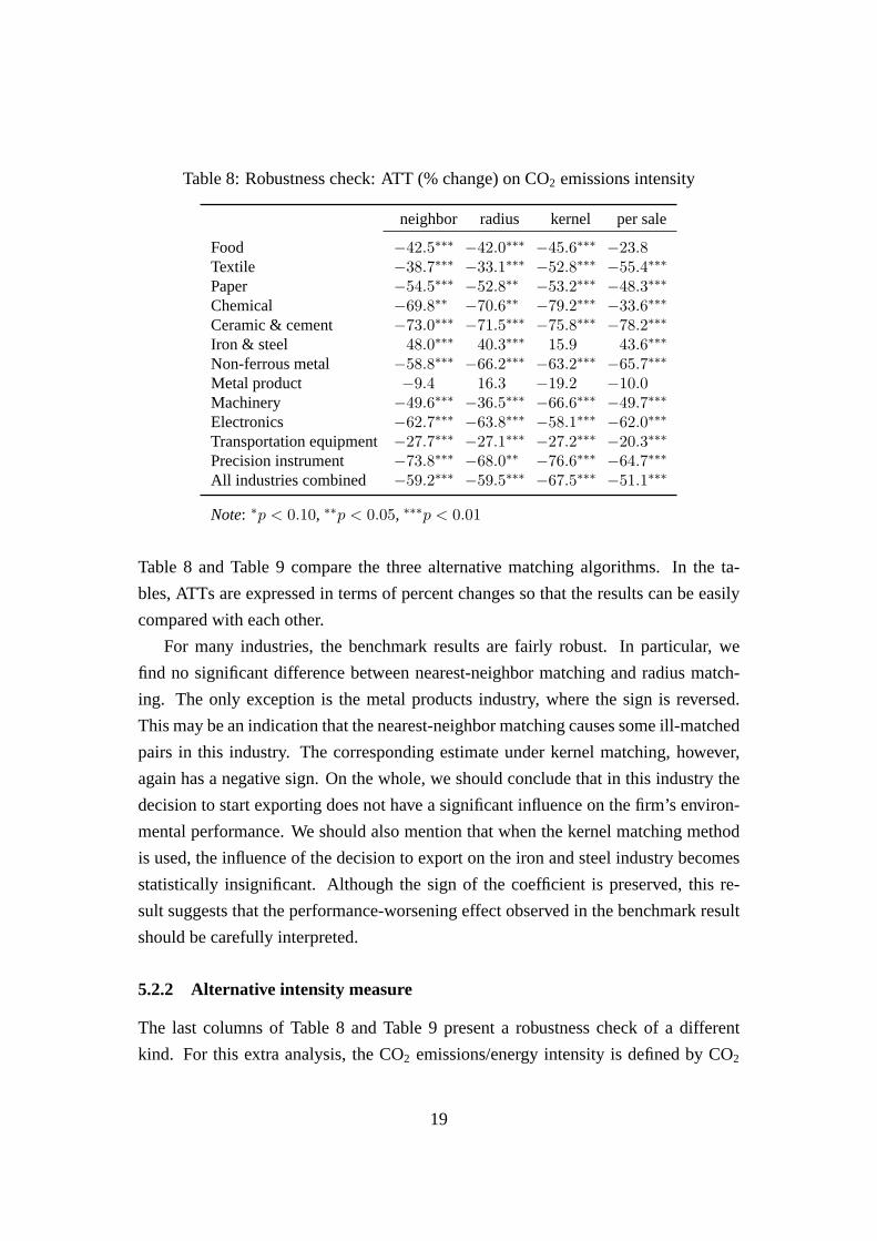
Table 8: Robustness check: ATT (% change) on CO2 emissions intensity
neighbor radius kernel per sale
Food −42.5∗∗∗ −42.0∗∗∗ −45.6∗∗∗ −23.8Textile −38.7∗∗∗ −33.1∗∗∗ −52.8∗∗∗ −55.4∗∗∗
Paper −54.5∗∗∗ −52.8∗∗ −53.2∗∗∗ −48.3∗∗∗
Chemical −69.8∗∗ −70.6∗∗ −79.2∗∗∗ −33.6∗∗∗
Ceramic & cement −73.0∗∗∗ −71.5∗∗∗ −75.8∗∗∗ −78.2∗∗∗
Iron & steel 48.0∗∗∗ 40.3∗∗∗ 15.9 43.6∗∗∗
Non-ferrous metal −58.8∗∗∗ −66.2∗∗∗ −63.2∗∗∗ −65.7∗∗∗
Metal product −9.4 16.3 −19.2 −10.0Machinery −49.6∗∗∗ −36.5∗∗∗ −66.6∗∗∗ −49.7∗∗∗
Electronics −62.7∗∗∗ −63.8∗∗∗ −58.1∗∗∗ −62.0∗∗∗
Transportation equipment−27.7∗∗∗ −27.1∗∗∗ −27.2∗∗∗ −20.3∗∗∗
Precision instrument −73.8∗∗∗ −68.0∗∗ −76.6∗∗∗ −64.7∗∗∗
All industries combined −59.2∗∗∗ −59.5∗∗∗ −67.5∗∗∗ −51.1∗∗∗
Note: ∗p < 0.10, ∗∗p < 0.05, ∗∗∗p < 0.01
Table 8 and Table 9 compare the three alternative matching algorithms. In the ta-
bles, ATTs are expressed in terms of percent changes so that the results can be easily
compared with each other.
For many industries, the benchmark results are fairly robust. In particular, we
find no significant difference between nearest-neighbor matching and radius match-
ing. The only exception is the metal products industry, where the sign is reversed.
This may be an indication that the nearest-neighbor matching causes some ill-matched
pairs in this industry. The corresponding estimate under kernel matching, however,
again has a negative sign. On the whole, we should conclude that in this industry the
decision to start exporting does not have a significant influence on the firm’s environ-
mental performance. We should also mention that when the kernel matching method
is used, the influence of the decision to export on the iron and steel industry becomes
statistically insignificant. Although the sign of the coefficient is preserved, this re-
sult suggests that the performance-worsening effect observed in the benchmark result
should be carefully interpreted.
5.2.2 Alternative intensity measure
The last columns of Table 8 and Table 9 present a robustness check of a different
kind. For this extra analysis, the CO2 emissions/energy intensity is defined by CO2
19

Table 9: Robustness check: ATT (% change) on energy intensity
neighbor radius kernel per sale
Food −41.8∗∗∗ −41.4∗∗∗ −43.8∗∗∗ −21.4Textile −35.9∗∗∗ −29.5∗∗∗ −50.4∗∗∗ −53.1∗∗∗
Paper −53.1∗∗∗ −52.3∗∗∗ −50.2∗∗∗ −47.5∗∗∗
Chemical −69.2∗∗ −69.9∗∗ −77.2∗∗∗ −28.9∗∗∗
Ceramic & cement −32.2∗∗ −31.8∗ −42.7∗∗∗ −43.0∗∗∗
Iron & steel 32.2∗∗∗ 28.6∗∗ 2.7 24.7∗∗∗
Non-ferrous metal −55.8∗∗∗ −63.8∗∗∗ −60.5∗∗∗ −62.8∗∗∗
Metal product −10.0 18.2 −19.9 −9.9Machinery −47.5∗∗∗ −36.7∗∗∗ −64.1∗∗∗ −48.7∗∗∗
Electronics −62.0∗∗∗ −63.1∗∗∗ −56.9∗∗∗ −62.1∗∗∗
Transportation equipment−25.9∗∗∗ −25.7∗∗∗ −25.8∗∗∗ −17.2∗∗
Precision instrument −76.6∗∗∗ −71.0∗∗ −79.0∗∗∗ −68.5∗∗∗
All industries combined −53.3∗∗∗ −54.0∗∗∗ −61.9∗∗∗ −36.7∗∗∗
Note: ∗p < 0.10, ∗∗p < 0.05, ∗∗∗p < 0.01
emissions and energy consumption per sale instead of per value added. We rerun the
same estimation procedure (with nearest-neighbor matching) as the benchmark result.
Since a different definition of intensity measure is used, the estimates listed in the last
column cannot be directly compared with those in the other columns. Nevertheless,
as the tables show, the results are qualitatively the same. Food industry is a notable
exception, for which the estimate is insignificant here. The overall impression is that
our benchmark estimates are not really sensitive to the definition of intensity measure.
6 Discussion
For many industries, we find robust evidence that exporting improves environmental
performance at the firm level. On average, firms are likely to become less CO2 emis-
sions/energy intensive once they decide to start exporting. This empirical finding is
consistent with the theoretical predictions provided by previous studies such as Cui et
al. (2012), Batrakova and Davies (2012), and Forslid et al. (2011).
A closer look at industry-level heterogeneity, however, yields that the magnitude
of the effect significantly varies across industries. Moreover, in some industries, our
empirical results suggest that exporting has no positive effect and may even worsen
firms’ environmental performance. In particular, firms in the iron and steel industry
become more CO2 emissions/energy intensive when they engage in exporting, indi-
20

cating that a different mechanism exists for this industry. Upon brief inspection of
the profile of the iron and steel industry, we realize that this is probably due to the
production process specific to this industry.8 Typically, the production of iron or steel
products can be divided into two distinct steps. In the first step, raw iron or steel is
produced using a (blast or electric) furnace, which is then processed into some inter-
mediate iron or steel products. This process involves a huge amount of CO2 emissions
and energy consumption but the products, if sold at this stage, usually have a low
market value. In the second step, the intermediate products are further processed into
finished iron or steel products, which often have a much higher market value. If firms
mainly export the products of the first step, which is actually the case for Japanese
firms, exporters will become, on the surface, more CO2 emissions/energy intensive
than non-exporters.
This discussion, although informal, suggests that if the effect of exporting on
environmental performance is to be accurately measured, a careful examination of
industry-specific production process is crucial. As Barrows and Ollivier (2014) point
out, exporting may change the firm’s product mix. For some industries, such a change
in product mix matters a lot since CO2 emissions/energy intensity can differ much
with product choice. If the decision to start exporting changes a firm’s product mix in
favor of emissions-intensive products, it partially offsets (or even completely masks)
the expected technology-upgrading effect. This is the possible underlying mechanism
for the iron and steel industry. Unfortunately, however, we are not able to disentangle
the technology-upgrading effect from the product-mix effect because our data set does
not allow us to control for the latter. The product-mix effect can work in the oppo-
site direction, too, if the firm’s product mix is rather tilted in favor of low-intensity
products. In fact, using a detailed data set of Indian manufacturing firms, Barrows and
Ollivier (2014) find that the technology-upgrading effect might not be as large as it
initially looks if changes in a firm’s product profile are appropriately controlled for.
Therefore, an important caveat to our empirical results is that the estimated effects
are not solely attributed to the technology upgradation facilitated by exporting. They
only capture the net impact of exporting, including the influence of possible changes
in the firm’s product mix.
8Our matching procedure is implemented based on the 2-digit industry code. We first suspectedthat there are some ill-matched pairs in this industry where, for example, firms with a blast furnace andthose with an electric furnace are compared. However, this is not the case. In reality, in Japan, there areonly four firms which own one or more blast furnaces, and these firms were omitted from our data setdue to missing values.
21

7 Conclusions
In this paper, we examined the firm-level relationship between export status and the
environmental performance in terms of CO2 emissions/energy intensity. We employed
Japanese firm-level data for the period 2006–2011. Using the PSM method, we rig-
orously analyzed whether exportingdoesimprove CO2 emissions/energy intensity.
We then found that on average exporting actually improves CO2 emissions/energy in-
tensity significantly. However, we also observed a large degree of heterogeneity in
this effect of exporting across industries. Whereas exporting improves CO2 emis-
sions/energy intensity in most industries, the PSM analysis resulted in an insignifi-
cant average effect of the treatment on the treated (ATT) in the metal products indus-
try. Moreover, in the iron & steel industry, exporting actuallyincreasesCO2 emis-
sions/energy intensity., which we suspect is due to a change in product composition
upon exporting.
Due to data limitations, we were unable to identify the mechanism behind the
above heterogeneity. Thus, in the future, we intend to further investigate the reason
why the relationship between export status and environmental performance differs
across industries.
References
Antweiler, W., B.R. Copeland, and M.S. Taylor (2001): “Is free trade good for the
environment?”American Economic Review, 91(4): 877-908.
Batrakova, S. and R.B. Davies (2012): “Is there an environmental benefit to being
an exporter? Evidence from firm-level data,”Review of World Economics148:
449-474.
Barrows, Geoffrey and Helene Ollivier (2014): “Does trade make firms cleaner?
Theory and evidence from Indian manufacturing.” Unpublished manuscript, UC
Berkeley.
Cole, Matthew A. and Robert J.R. Elliot (2003): “Determining the trade-environment
composition effect: the role of capital, labor and environmental regulations,”
Journal of Environmental Economics and Management, 46: 363–383.
22

Copeland, Brian R. and M. Scott Taylor (1994): “North-South trade and the environ-
ment,”Quarterly Journal of Economics, 109(3): 755–787.
Copeland, Brian R. and M. Scott Taylor (2003):Trade and the Environment: Theory
and Evidence. Princeton: Princeton University Press.
Copeland, Brian R. and M. Scott Taylor (2004): “Trade, growth, and the environ-
ment,”Journal of Economic Literature, 42: 7–71.
Cui, J., H. Lapan, and G. Moschini (2012): “Are exporters more environmentally
friendly than non-exporters? Theory and evidence,” Working Paper No. 12022.
Department of Economics, Iowa State University.
De Loecker J. and F. Warzynski (2012): “Markups and firm-level export status,”
American Economic Review, 102(6): 2437–2471.
Forslid, R., T. Okubo, and K.H.Ulltveit-Moe (2011): “International trade, CO2 emis-
sions and heterogeneous firms.” CEPR Discussion Paper No. 8583.
Grossman, Gene M. and Alan B. Krueger (1993): “Environmental impacts of a North
American Free Trade Agreement,” in Garber, P.M. ed.The U.S.-Mexico Free
Trade Agreement. Cambridge, MA: MIT Press, pp. 13–56.
Managi, S., A. Hibiki, and T. Tsurumi (2009) “Does trade openness improve en-
vironmental quality?”Journal of Environmental Economics and Management,
58: 346–363.
Melitz, M. (2003): “The impact of trade on intra-industry reallocations and aggregate
industry productivity,”Econometrica, 71(6):1695–1725.
Rosenbaum, P.R. and D.B. Rubin (1983): “The central role of the propensity score
in observational studies for causal effects,”Biometrika, 70(1):41–55.
Rubin, D.B. (1974): “Estimating causal effects of treatments in randomized and non-
randomized studies,”Journal of Educational Psychology, 66(5):688–701.
Rubin, D.B. (2001): “Using propensity scores to help design observational studies:
application to the tobacoo litigation,”Health Services & Outcomes Research
Methodology, 2:169–188.
23
Tanaka, A. (2013): “The causal effects of exporting on domestic workers: a firm-
level analysis using Japanese data,”Japan and the World Economy, 28:13–23.
A Appendix
A.1 Productivity estimation
To estimate the total factor productivity, we consider a translog production function of
the form
yi,t = ωi,t + βlli,t + βkki,t + βlll2i,t + βkkk
2i,t + βlkli,tki,t, (5)
whereyi,t is value added,li,t is labor, andki,t is capital, all in logarithmic value.
Following De Loecker and Warzynski (2013), we first run the OLS regression on
yi,t = ϕt(li,t, ki,t, ei,t, di,t, , ri,t) + ϵi,t, (6)
whereei,t is energy consumption,di,t is an export dummy, andri,t is R&D inten-
sity. We approximateϕt(·) with a second-order polynomial series. Having obtained
estimatesϕi,t of expected output, we can compute
ωi,t(β) = ϕi,t − βlli,t − βkki,t − βlll2i,t − βkkk
2i,t − βlkli,tki,t (7)
for any candidate valueβ = (βl, βk, βll, βkk, βlk). We then run the regression
ωi,t(β) = gt(ωi,t−1(β)) + ξi,t, (8)
wheregt(·) is approximated with a third-order polynomial. This in turn allows us to
recover the associated estimatesξi,t(β) of innovation as
ξi,t(β) = ωi,t(β)− gi,t(β). (9)
The estimate ofβ for the production function is obtained by the standard GMM tech-
nique with the moment condition
E[ξi,t(β)zi,t
]= 0, (10)
24

Table 10: Estimated translog production function
βl βll βk βkk βlk
Food 0.76 −0.05 −1.44 0.11 0.04Textile 0.68 0.08 −0.96 0.09 −0.07Paper 1.79 0.13 0.13 0.08 −0.24Chemical 0.52 0.04 −0.29 0.06 −0.05Ceramic & cement 0.75 0.06 0.25 0.04 −0.09Iron & steel 1.10 −0.07 −0.55 0.05 0.03Non-ferrous metal 0.24 0.14 0.86 0.01 −0.15Metal product 0.62 0.06 0.11 0.04 −0.08Machinery 1.21 0.01 −0.91 0.08 −0.06Electronics 0.49 0.11 0.13 0.06 −0.14Trans. eqpt 0.78 0.13 0.27 0.09 −0.22Precision inst. −1.30 0.30 −0.93 0.16 −0.25
where
zi,t = (li,t−1, ki,t, l2i,t−1, k
2i,t, ki,tli,t−1)
T . (11)
Table 10 reports the estimation results. Once estimateβ is obtained, the estimated
total factor productivity in logarithmic value is given by
ωi,t = yi,t − βlli,t − βkki,t − βlll2i,t − βkkk
2i,t − βlkli,tki,t. (12)
25

Table 11: OLS on log CO2 emission intensity (industry-wise decomposition)
Food Textile Paper Chemical
EXPORTER −0.374∗∗∗ −0.573∗∗∗ −0.266 −0.344∗∗∗
(0.058) (0.097) (0.187) (0.061)EXPSHARE 0.227 2.285∗∗∗ 1.938 0.645∗∗
(0.456) (0.812) (1.561) (0.273)ln TFP −0.883∗∗∗ −0.405∗∗∗ −0.033 −0.809∗∗∗
(0.032) (0.061) (0.114) (0.044)ln LABOR −0.476∗∗∗ −0.095 −0.038 −0.384∗∗∗
(0.022) (0.068) (0.065) (0.032)RDINT −0.220∗∗ −0.331∗∗ −0.666∗∗ −0.586∗∗∗
(0.093) (0.135) (0.329) (0.108)Observation 1266 324 294 1554R squared 0.541 0.554 0.345 0.537
Ceramic & cement Iron & Steel Non-ferrous metal Metal product
EXPORTER −0.365∗∗ −0.017 −0.481∗∗∗ 0.108(0.145) (0.091) (0.103) (0.096)
EXPSHARE −0.083 0.935∗∗ −0.890∗∗ −1.227∗∗
(0.565) (0.430) (0.400) (0.506)ln TFP 0.013 −0.490∗∗∗ −0.621∗∗∗ −0.765∗∗∗
(0.107) (0.073) (0.084) (0.070)ln LABOR −0.531∗∗∗ −0.023 −0.137∗∗ −0.671∗∗∗
(0.090) (0.053) (0.059) (0.049)RDINT −0.945∗∗∗ −0.452 0.541∗∗ 0.112
(0.298) (0.279) (0.215) (0.208)Observation 468 618 378 312R squared 0.286 0.128 0.444 0.601
Machinery Electronics Trans. eqpt Precision inst.
EXPORTER −0.235∗∗∗ −0.445∗∗∗ −0.149∗∗ −0.215(0.087) (0.068) (0.062) (0.153)
EXPSHARE −0.529∗∗∗ −0.125 0.483∗∗ 0.123(0.164) (0.213) (0.230) (0.348)
ln TFP −0.947∗∗∗ −0.524∗∗∗ −0.829∗∗∗ −0.833∗∗∗
(0.075) (0.048) (0.053) (0.135)ln LABOR −0.521∗∗∗ −0.256∗∗∗ −0.158∗∗∗ −0.698∗∗∗
(0.044) (0.028) (0.033) (0.096)RDINT −0.234 −0.454∗∗∗ −0.336∗∗∗ 0.391
(0.144) (0.102) (0.117) (0.272)Observation 390 966 924 168R squared 0.666 0.377 0.294 0.753
Note: The values in parentheses are standard errors. Observations with miss-ing values are dropped.∗p < 0.10, ∗∗p < 0.05, ∗∗∗p < 0.01.
26

Table 12: OLS on log energy intensity (industry-wise decomposition)
Food Textile Paper Chemical
EXPORTER −0.367∗∗∗ −0.604∗∗∗ −0.269 −0.293∗∗∗
(0.058) (0.097) (0.183) (0.059)EXPSHARE 0.336 3.262∗∗∗ 2.025 0.580∗∗
(0.453) (0.807) (1.528) (0.265)ln TFP −0.868∗∗∗ −0.405∗∗∗ −0.034 −0.821∗∗∗
(0.032) (0.061) (0.112) (0.042)ln LABOR −0.456∗∗∗ −0.148∗∗ −0.015 −0.364∗∗∗
(0.022) (0.068) (0.063) (0.031)RDINT −0.215∗∗ −0.234∗ −0.543∗ −0.527∗∗∗
(0.093) (0.134) (0.322) (0.105)Observation 1266 324 294 1554R squared 0.532 0.573 0.341 0.533
Ceramic & cement Iron & Steel Non-ferrous metal Metal product
EXPORTER −0.115 −0.037 −0.477∗∗∗ 0.100(0.116) (0.087) (0.102) (0.096)
EXPSHARE −0.328 0.823∗∗ −0.914∗∗ −1.231∗∗
(0.453) (0.409) (0.398) (0.506)ln TFP −0.252∗∗∗ −0.516∗∗∗ −0.597∗∗∗ −0.805∗∗∗
(0.086) (0.070) (0.083) (0.070)ln LABOR −0.482∗∗∗ −0.041 −0.153∗∗∗ −0.669∗∗∗
(0.072) (0.050) (0.058) (0.049)RDINT −0.861∗∗∗ −0.426 0.619∗∗∗ 0.160
(0.239) (0.266) (0.214) (0.208)Observation 468 618 378 312R squared 0.263 0.146 0.429 0.607
Machinery Electronics Trans. eqpt Precision inst.
EXPORTER −0.262∗∗∗ −0.422∗∗∗ −0.150∗∗ −0.220(0.087) (0.067) (0.061) (0.153)
EXPSHARE −0.467∗∗∗ −0.117 0.412∗ 0.189(0.164) (0.209) (0.227) (0.347)
ln TFP −0.945∗∗∗ −0.531∗∗∗ −0.822∗∗∗ −0.864∗∗∗
(0.074) (0.047) (0.052) (0.134)ln LABOR −0.495∗∗∗ −0.268∗∗∗ −0.150∗∗∗ −0.694∗∗∗
(0.044) (0.027) (0.033) (0.096)RDINT −0.245∗ −0.437∗∗∗ −0.274∗∗ 0.466∗
(0.143) (0.100) (0.116) (0.271)Observation 390 966 924 168R squared 0.663 0.378 0.294 0.754
Note: The values in parentheses are standard errors. Observations with miss-ing values are dropped.∗p < 0.10, ∗∗p < 0.05, ∗∗∗p < 0.01.
27


