

Double Trouble: The Problem with Double Deflation of Value Added, and an Input-Output Alternative with an Application to
Russia
Clopper Almon1
Many, perhaps all, statistical offices prepare constant-price value added for various economic sectors (or "industries") by the double-deflation method. These figures are then used to study productivity changes in the different sectors. I have long argued that this method makes no economic sense and can lead to ridiculous results. Indeed, I know of no defensible way to measure productivity gains within a single industry. It is, however, possible to measure changes in the efficiency of the whole economy in producing various products for final demand. This note explains and illustrates the problem with double deflation, describes the input-output based alternative, and applies it to the Russian economy in the period 1980 - 2006 on the basis of a remarkable data set developed by Marat Uzyakov. The application portion of the paper should be thought of as an internal discussion paper within the international Inforum group.
The Problem Double Deflation was Supposed to Solve Economic progress depends on increases in productivity, so there is naturally a desire to
identify the industries in which it is occurring and to measure its growth in those industries. Simple measures such as (a) industry output in constant prices divided by labor input in hours or (b) industry output in constant prices divided by all value added in the industry deflated by the GDP deflator fail to deal with the possibly important phenomenon of out sourcing. For example, in a base year, television sets may have been built in a factory that made the cabinet, the tube, and the electronics. In a later year, the typical TV factory may have bought the cabinet, tube, and electronics, and merely assembled the unit. If we measured the productivity by just the gross output divided by the primary inputs, we would find a large increase in productivity, which would be totally misleading. The use of intermediate inputs must somehow be taken into account in measuring productivity. Double deflation is one attempt to do so.
Double-Deflation and its Problems
To get double-deflated value added, one deflates the output of a sector and then from it subtracts the deflated value of intermediate inputs. (If there is no input-output table for the year in question or if current-price value-added data is not consistent with the input-output table, the method is modified to fit the situation. We will assume the ideal case of an available, matching input-output table and ignore these modifications.) The tables on the following page illustrate the method applied in three different cases. In all cases, we assume an economy with two sectors with production and consumption functions of the Cobb-Douglas form so that, as prices change, the nominal shares of each input remain constant, as do their shares in final demand. The first table shown can therefore characterize the economy in both year 1 and year 2. We may let both prices be
1 The author is professor of economics emeritus at the University of Maryland. This paper for the 2008 Inforum
World Conference is a continuation of work begun in May of this year when I had the privilege to be the guest of the Institute of Economic Forecasting of the Russian Academy of Sciences. The data used was developed by Marat Uzyakov of that Institute. I am solely responsible for the opinions and the calculations. They have NOT been reviewed by Uzyakov or others of that institute.
1

1.0 in year 1.
2

These examples assume a Cobb-Douglas production function so thatnominal shares remain constant as prices change.Input-Output Table in current prices for both year 1 and year 2.
Sector 1 Sector 2 Final demand Output PricesSector 1 0.0 40.0 60.0 100.0 1.0Sector 2 40.0 0.0 60.0 100.0 1.0Value added 60.0 60.0
Case 1: In year 2, both prices fall to .5Table for year 1, prices of year 2
Sector 1 0.0 20.0 30.0 50.0 0.5Sector 2 20.0 0.0 30.0 50.0 0.5DD Value added 30.0 30.0VA growth ratio 2.0 2.0
Table for year 2, prices of year 1Sector 1 0.0 80.0 120.0 200.0Sector 2 80.0 0.0 120.0 200.0DD Value added 120.0 120.0VA growth ratio 2.0 2.0
2.0 2.0
Case 2: In year 2, price of product 1 rises to 1.10; price of product 2 falls to 0.90 Table for year 1, prices of year 2
Sector 1 0.0 44.0 66.0 110.0 1.1Sector 2 36.0 0.0 54.0 90.0 0.9DD Value added 74.0 46.0VA growth ratio 0.81 1.30
Table for year 2, prices of year 1Sector 1 0.0 36.4 54.5 90.9 1.1Sector 2 44.4 0.0 66.7 111.1 0.9DD Value added 46.5 74.7VA growth ratio 0.77 1.25
0.79 1.27
Case 3: In year 2, price of product 1 doubles, of product 2, falls to .5Table for year 1, prices of year 2
Sector 1 0.0 80.0 120.0 200.0 2.0Sector 2 20.0 0.0 30.0 50.0 0.5DD Value added 180.0 -30.0VA growth ratio 0.33 -2.00
Table for year 2, prices of year 1Sector 1 0.0 20.0 30.0 50.0 2.0Sector 2 80.0 0.0 120.0 200.0 0.5DD Value added -30.0 180.0VA growth ratio -0.50 3.00
GeoMeanRatio
GeoMeanRatio
GeoMeanRatio 0.41i 2.45i
3

In Case 1, both prices fall to 0.5 in year 2. The first table under this case shows the first year's table deflated to prices of the second year, while the second table shows the second year's table in prices of the first year. Whichever deflated table we use, we find that real value added has doubled in each industry. This is clearly the right answer for this case.
In Case 2, the price of product 1 rises to 1.1 while that of product 2 falls to .9 in year 2. In this case, as in most cases of differing rates of change of the prices, the growth ratio for double-deflated value added depends upon whether one deflates year 1 by prices of year 2 (Paasche indexes) or year 2 with prices of year 1 (Laspeyers indexes). The usual resolution is to determine the growth ratio as the geometric mean of the two. These means are shown in the last line of the case. In year 2, "real" GDP originating in sector 1 falls to 79 percent of its value in year 1, while it rises in sector 2 to 127 percent of its base year value. I shall argue that, already in this case, these growth rates are nonsense, statistical muck, although that fact is not yet patently obvious.
In Case 3, the price of product 1 rises to 2.0 while that of product 2 falls to 0.5 in year 2. Year 1 in prices of year 2 shows negative value added in sector 2, while year 2 in prices of year 1 shows negative value added in sector 1. The geometric mean growth ratio of double-deflated value added for sector 1 is 0.41i and for sector 2, 2.45i, where i is the unit imaginary number, the square root of -1 in the complex numbers. I must emphasize that this case is developed in the framework most commonly used for illustrations of production functions. In fact, it is not necessary to go to such extreme price differences to get imaginary growth ratios; our example gives them when the price of product 1 goes up to 1.6 and that of product 2 falls to 0.62 in the second year. Anyone who believes that double deflation is an appropriate way to deflate value added should be prepared to explain the economic meaning of these imaginary growth ratios. I would rather not have to do so.
In my own view, the imaginary growth rates are only the reductio ad absurdum of a method that makes no sense no matter how small the price changes. The first consideration is the matter of units. Some operations with input-output tables make sense with all of the products measured in physical units. Leontief himself liked to think in physical units and often asked speakers in his seminar to give examples in physical units. The column sums of a table in physical units, however, make no sense whatsoever. When we put a flow table of one year, say t, into prices of some other year, say T, we are essentially putting the table into physical units. The unit for each row is how much a dollar (or euro, or ruble, or other currency unit) would have bought of the product in that row in year T. The column sums of such a table are therefore conceptually suspect. The sum of column j tells us how much the inputs bought by industry j in year t would have cost in year T, but that magnitude has no necessary relation to output of j in year t measured in prices of year T. The first may be less than, equal to, or greater than the second, as shown in our examples. No economic significance can therefore be attached to their difference. But that difference is precisely the double-deflated value added.
Another way to see the fallacy of double deflation is to consider the case in which the primary inputs can be deflated. Suppose there is only one primary input, labor, and that all value added is payment to labor, and that there is a good deflator for labor. We could then add labor to the list of inputs and subtract the total cost of all inputs in year t, measured in prices of year T, from the output in year t, measured in prices of year T. Clearly, there is no reason to expect that this difference should be zero. It is not the return to any factor, because all factors have been accounted for. It is just statistical muck. Suppose that we now add to this muck the return to labor. But muck + anything = muck. Thus double-deflated value added is always muck.
The lamest defense of double deflation is to say that if it is done in small steps, the imaginary growth ratios do not in practice appear. Of course they don't; the nonsense of any ridiculous method will not appear if the changes are minute.
4

Double deflated value add is a statistic which should never be calculated; and, if calculated, should not be released; and, if released, should never be used if there is anything more reasonable available.
Nevertheless, the deflated output which goes into the computation of deflated value added is an important statistic and should be calculated and released.
The Input-Output Alternative to Double Deflation If there is a satisfactory way to pinpoint productivity change in specific industries, I do not
know what it is. There is, however, a way to identify productivity change in the way the whole economy makes a particular product. We just need to calculate how many resources go into delivering one unit of each product to final demand in each year. The unit of product should, of course, be the same in all years.
To explain the calculation, we need a bit of notation. For each year t, t = 0, ..., T, let:
At be the input-output coefficient matrix of year t,
vt be the vector of value real input per unit of output in year t
pt be the vector of prices in year t; in year 0, all prices are 1.0.
Now recall that column j of the Leontief inverse, (I - A)-1 , shows the outputs necessary, directly and indirectly, to produce one unit of final demand of product j. Thus
xt = vt'(I - At )-1
is the vector of real inputs per unit of final demand produced in year t. The unit of final demand, however, is the output of one currency unit (ruble, dollar, euro, and so on) of the product. This unit gets smaller as prices increase, so to convert the x vector to a constant unit, we need to multiply it element-by-element by the price index vector. Thus
zt = xt*pt
will give the desired vector of real inputs needed to produce a (constant-sized) unit of final output of each problem.
Increasing productivity in a producing the final demand in indicated by a decline in the resources necessary to produce it.
These calculations assume that imports are made with the same input patterns as the domestic product. This assumption could be replaced with the assumption that imports are produced with exports, but that has not been done here.
Notice that this method fully takes into account changes in the input output coefficients. It would make perfect sense if all or some products in the input-output table were measured in physical units -- as indeed they are when we put the table of year 2 into prices of year 1. It takes into account increased labor productivity and changes in capital intensity. It makes no use of adding up numbers in different units.
Application to Russia The data set mentioned above contains 44-sector input-output tables for the period 1980-2006.
Given this set of comparable tables in current prices, the main problem in the application of the method described above lies in determining real inputs. My idea was to begin by determining the total employment in the economy and to increase it by the ratio of total value added to wages plus
5

half of mixed income. Thus, we assume that employment represents the real input of labor while the rest of value added represents the real input of capital and other factors. In principle, this employment should be adjusted for quality, but I have made no such adjustment in the calculations shown here. These total real resources were then allocated among industries in each year in proportion to value added in that year.
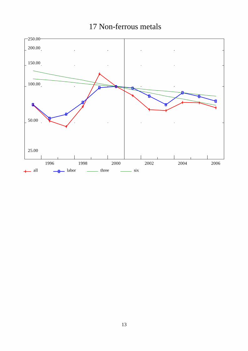
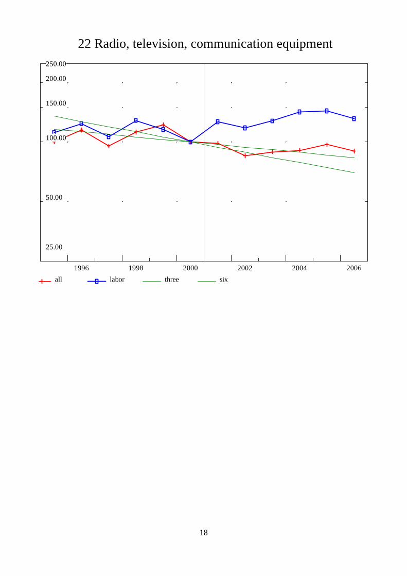
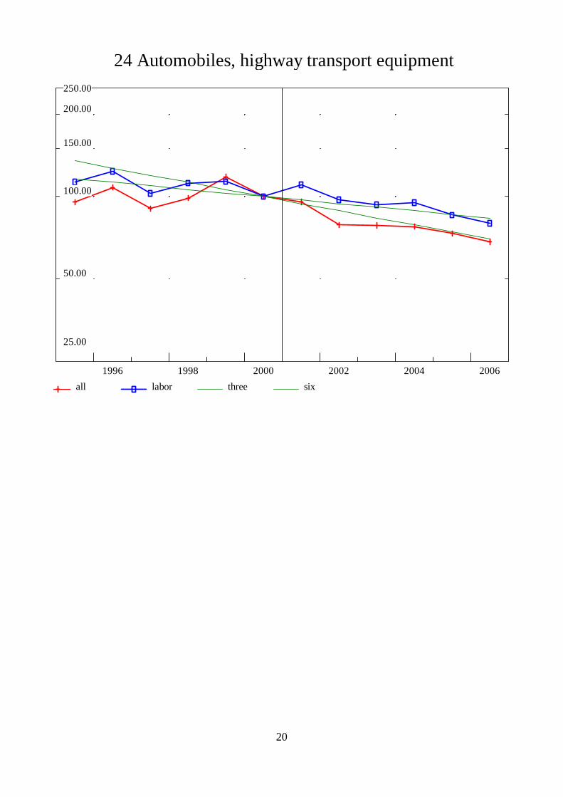
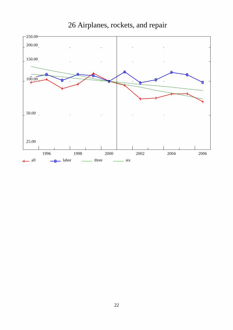
Most of the peculiarities in the results stem from the inadequacies of this procedure. I have taken the capital input to be gross profits. But in some cases, profits were negative. Surely, that does not mean that the input of capital was negative. A measure of capital input on the basis of the capital stock would give more reasonable and stable results. Taxes on products are a somewhat peculiar primary input, all the more so when they are negative, representing subsidies. Because of these peculiarities of profits and taxes, a second computation was made using only compensation of employees plus mixed income to distribute employment among industries. In the graphs shown below, the results of the first computation are shown by the (red) line marked by + signs, while the second are shown by the (blue) line marked by squares. Both have been normalized to be 100 in the year 2000. Many of the series showed a substantial discontinuity in 1995, the year of an input-output table important for the construction of the subsequent tables. For this reason, the graphs have been limited to the period beginning in 1995, where the data seems fairly consistent from year to year. 1995 is also the first year for which we have direct information on employment. Data for earlier years was based on population in the working age groups.
Many products showed an upward jump in resource requirements to produce a unit of final demand -- a negative change in productivity -- after the end of the Soviet Union, and even after 1995. That result came about because output fell faster than employment in many industries. Beginning about 1999, most products begin to show steady declines in resource requirements.
For reference, lines showing a 3 percent per year and a 6 percent per year decline have been included in the graphs, which use a logarithmic vertical scale.
In the 2000 - 2006 period, most products showed fairly high rates of reduction of input requirements. The fastest growth in productivity was in Communications (9.2 per cent per year), Business services (6.5), Construction (4.7), and Agriculture (4.3). Between 3 and 4 percent per year were Trade, Computers, Real estate, Hotels and restaurants, Electrical appliances, Fabricated metal products, Ships, and Aircraft. Productivity in automobiles rose at 2.8 percent per year. Generally, the reduction in resource use based on all components of value added was faster than that based only on wage and mixed income.
While not without problems in implementation, the resource content of final demand approach to productivity measurement seems to offer a feasible and certainly conceptually superior alternative to the currently dominant double-deflated value added method.
6

1 Agriculture 1 Agriculture
25.00
50.00
100.00
150.00
200.00
250.00
1996 1998 2000 2002 2004 2006 all labor three six
2 Petroleum extraction2 Petroleum extraction
25.00
50.00
100.00
150.00
200.00
250.00
1996 1998 2000 2002 2004 2006 all labor three six
3 Natural gas extraction 3 Natural gas extraction
25.00
50.00
100.00
150.00
200.00
250.00
1996 1998 2000 2002 2004 2006 all labor three six
4 Coal mining4 Coal mining
25.00
50.00
100.00
150.00
200.00
250.00
1996 1998 2000 2002 2004 2006 all labor three six
5 Other Fuels, incl. nuclear 5 Other Fuels, incl. nuclear
25.00
50.00
100.00
150.00
200.00
250.00
1996 1998 2000 2002 2004 2006 all labor three six
6 Ores and other mining6 Ores and other mining
25.00
50.00
100.00
150.00
200.00
250.00
1996 1998 2000 2002 2004 2006 all labor three six
7 Food, beverages, tobacco 7 Food, beverages, tobacco
25.00
50.00
100.00
150.00
200.00
250.00
1996 1998 2000 2002 2004 2006 all labor three six
8 Textiles, apparel, leather8 Textiles, apparel, leather
25.00
50.00
100.00
150.00
200.00
250.00
1996 1998 2000 2002 2004 2006 all labor three six
7

9 Wood and wood products 9 Wood and wood products
25.00
50.00
100.00
150.00
200.00
250.00
1996 1998 2000 2002 2004 2006 all labor three six
10 Paper and printing10 Paper and printing
25.00
50.00
100.00
150.00
200.00
250.00
1996 1998 2000 2002 2004 2006 all labor three six
11 Petroleum refining 11 Petroleum refining
25.00
50.00
100.00
150.00
200.00
250.00
1996 1998 2000 2002 2004 2006 all labor three six
12 Chemicals12 Chemicals
25.00
50.00
100.00
150.00
200.00
250.00
1996 1998 2000 2002 2004 2006 all labor three six
8

13 Pharmaceuticals 13 Pharmaceuticals
25.00
50.00
100.00
150.00
200.00
250.00
1996 1998 2000 2002 2004 2006 all labor three six
9

14 Plastic products 14 Plastic products
25.00
50.00
100.00
150.00
200.00
250.00
1996 1998 2000 2002 2004 2006 all labor three six
10

15 Stone, Clay, and Glass products 15 Stone, Clay, and Glass products
25.00
50.00
100.00
150.00
200.00
250.00
1996 1998 2000 2002 2004 2006 all labor three six
11

16 Ferrous metals 16 Ferrous metals
25.00
50.00
100.00
150.00
200.00
250.00
1996 1998 2000 2002 2004 2006 all labor three six
12
17 Non-ferrous metals 17 Non-ferrous metals
25.00
50.00
100.00
150.00
200.00
250.00
1996 1998 2000 2002 2004 2006 all labor three six
13

18 Fabricated metal products18 Fabricated metal products
25.00
50.00
100.00
150.00
200.00
250.00
1996 1998 2000 2002 2004 2006 all labor three six
14

19 Machinery 19 Machinery
25.00
50.00
100.00
150.00
200.00
250.00
1996 1998 2000 2002 2004 2006 all labor three six
15

19 Machinery 19 Machinery
25.00
50.00
100.00
150.00
200.00
250.00
1996 1998 2000 2002 2004 2006 all labor three six
20 Computers, office machinery 20 Computers, office machinery
25.00
50.00
100.00
150.00
200.00
250.00
1996 1998 2000 2002 2004 2006 all labor three six
16

21 Electical apparatus 21 Electical apparatus
25.00
50.00
100.00
150.00
200.00
250.00
1996 1998 2000 2002 2004 2006 all labor three six
17
22 Radio, television, communication equipment 22 Radio, television, communication equipment
25.00
50.00
100.00
150.00
200.00
250.00
1996 1998 2000 2002 2004 2006 all labor three six
18

23 Medical, optical, and precision instruments 23 Medical, optical, and precision instruments
25.00
50.00
100.00
150.00
200.00
250.00
1996 1998 2000 2002 2004 2006 all labor three six
19
24 Automobiles, highway transport equipment 24 Automobiles, highway transport equipment
25.00
50.00
100.00
150.00
200.00
250.00
1996 1998 2000 2002 2004 2006 all labor three six
20

25 Sea transport equipment and its repair 25 Sea transport equipment and its repair
25.00
50.00
100.00
150.00
200.00
250.00
1996 1998 2000 2002 2004 2006 all labor three six
21
26 Airplanes, rockets, and repair 26 Airplanes, rockets, and repair
25.00
50.00
100.00
150.00
200.00
250.00
1996 1998 2000 2002 2004 2006 all labor three six
22

26 Airplanes, rockets, and repair 26 Airplanes, rockets, and repair
25.00
50.00
100.00
150.00
200.00
250.00
1996 1998 2000 2002 2004 2006 all labor three six
23

27 Railroad equipment and its repair 27 Railroad equipment and its repair
25.00
50.00
100.00
150.00
200.00
250.00
1996 1998 2000 2002 2004 2006 all labor three six
24

28 Recycling 28 Recycling
25.00
50.00
100.00
150.00
200.00
250.00
1996 1998 2000 2002 2004 2006 all labor three six
25

29 Electric, gas, and water utilities 29 Electric, gas, and water utilities
25.00
50.00
100.00
150.00
200.00
250.00
1996 1998 2000 2002 2004 2006 all labor three six
26

30 Construction 30 Construction
25.00
50.00
100.00
150.00
200.00
250.00
1996 1998 2000 2002 2004 2006 all labor three six
27

31 Wholesale and retail trade31 Wholesale and retail trade
25.00
50.00
100.00
150.00
200.00
250.00
1996 1998 2000 2002 2004 2006 all labor three six
28

32 Hotels and restaurants 32 Hotels and restaurants
25.00
50.00
100.00
150.00
200.00
250.00
1996 1998 2000 2002 2004 2006 all labor three six
29

33 Transport and storage 33 Transport and storage
25.00
50.00
100.00
150.00
200.00
250.00
1996 1998 2000 2002 2004 2006 all labor three six
30
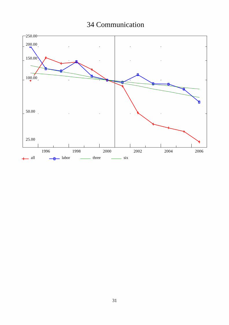
34 Communication 34 Communication
25.00
50.00
100.00
150.00
200.00
250.00
1996 1998 2000 2002 2004 2006 all labor three six
31

35 Finance and insurance 35 Finance and insurance
25.00
50.00
100.00
150.00
200.00
250.00
1996 1998 2000 2002 2004 2006 all labor three six
32

36 Real estate 36 Real estate
25.00
50.00
100.00
150.00
200.00
250.00
1996 1998 2000 2002 2004 2006 all labor three six
33
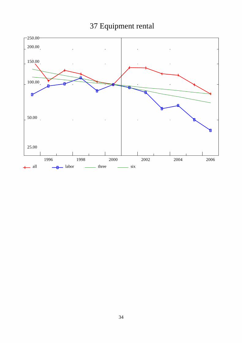
37 Equipment rental 37 Equipment rental
25.00
50.00
100.00
150.00
200.00
250.00
1996 1998 2000 2002 2004 2006 all labor three six
34

38 Computing service 38 Computing service
25.00
50.00
100.00
150.00
200.00
250.00
1996 1998 2000 2002 2004 2006 all labor three six
35

39 Research and development39 Research and development
25.00
50.00
100.00
150.00
200.00
250.00
1996 1998 2000 2002 2004 2006 all labor three six
36

40 Other business services 40 Other business services
25.00
50.00
100.00
150.00
200.00
250.00
1996 1998 2000 2002 2004 2006 all labor three six
37

41 Government, defense, social insurance 41 Government, defense, social insurance
25.00
50.00
100.00
150.00
200.00
250.00
1996 1998 2000 2002 2004 2006 all labor three six
38

42 Education 42 Education
25.00
50.00
100.00
150.00
200.00
250.00
1996 1998 2000 2002 2004 2006 all labor three six
39

43 Health services 43 Health services
25.00
50.00
100.00
150.00
200.00
250.00
1996 1998 2000 2002 2004 2006 all labor three six
40
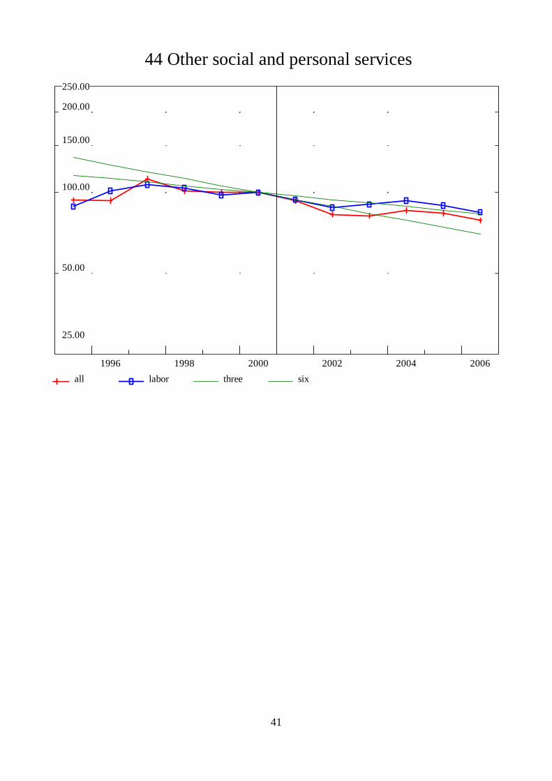
44 Other social and personal services 44 Other social and personal services
25.00
50.00
100.00
150.00
200.00
250.00
1996 1998 2000 2002 2004 2006 all labor three six
41


