
General rights Copyright and moral rights for the publications made accessible in the public portal are retained by the authors and/or other copyright owners and it is a condition of accessing publications that users recognise and abide by the legal requirements associated with these rights.
• Users may download and print one copy of any publication from the public portal for the purpose of private study or research. • You may not further distribute the material or use it for any profit-making activity or commercial gain • You may freely distribute the URL identifying the publication in the public portal
If you believe that this document breaches copyright please contact us providing details, and we will remove access to the work immediately and investigate your claim.
Downloaded from orbit.dtu.dk on: Jun 17, 2018
Dynamic Modeling, Optimization, and Advanced Control for Large Scale Biorefineries
Prunescu, Remus Mihail; Blanke, Mogens; Sin, Gürkan; Jensen, Jakob Munch; Jakobsen, Jon Geest
Publication date:2015
Document VersionPublisher's PDF, also known as Version of record
Link back to DTU Orbit
Citation (APA):Prunescu, R. M., Blanke, M., Sin, G., Jensen, J. M., & Jakobsen, J. G. (2015). Dynamic Modeling, Optimization,and Advanced Control for Large Scale Biorefineries. Technical University of Denmark, Department of ElectricalEngineering.

Remus Mihail Prunescu
Dynamic Modeling, Optimization,and Advanced Control for LargeScale Biorefineries
PhD Thesis, November 2015

DynamicModeling, Optimization,and Advanced Control for Large
Scale Biorefineries
Remus Mihail Prunescu
Technical University of DenmarkKgs. Lyngby, Denmark, 2015

Technical University of DenmarkAutomation and Control (AUT)Elektrovej Building 326DK-2800, Kgs. LyngbyDenmarkPhone: (+45) 45 25 35 76Email: [email protected]
ISBN: N/A
Summary
Second generation biorefineries transform agricultural wastes into biochemicals
with higher added value, e.g. bioethanol, which is thought to become a primary
component in liquid fuels [1]. Extensive endeavors have been conducted to make
the production process feasible on a large scale, and recently several commercial size
biorefineries became operational: Beta Renewables (Italy, 2014), Abengoa Bioenergy
(USA, 2014), POET-DSM (USA, 2014), GranBio (Brazil, 2014) [2], while others are
under construction, e.g. the Måbjerg Energy Consortium in Denmark.
This thesis presents the findings of a 3 years PhD project that was run by Techni-
cal University of Denmark (DTU) in collaboration with the largest Danish energy
company DONG Energy A/S between 2012 and 2015. The company owns a demon-
stration scale second generation biorefinery in Kalundborg, Denmark, also known
as the Inbicon demonstration plant [3]. The goal of the project is to utilize real-
time data extracted from the large scale facility to formulate and validate first
principle dynamic models of the plant. These models are then further exploited to
derive model-based tools for process optimization, advanced control and real-time
monitoring.
The Inbicon biorefinery converts wheat straw into bioethanol utilizing steam,
enzymes, and genetically modified yeast. The biomass is first pretreated in a steam
pressurized and continuous thermal reactor where lignin is relocated, and hemicel-
lulose partially hydrolyzed such that cellulose becomes more accessible to enzymes.
The biorefinery is integrated with a nearby power plant following the Integrated
Biomass Utilization System (IBUS) principle for reducing steam costs [4]. During
the pretreatment, by-products are also created such as organic acids, furfural, and
pseudo-lignin, which act as inhibitors in downstream processes. The pretreated
fibers consist of cellulose and xylan, which are then liquefied in the enzymatic
hydrolysis process with the help of enzymes. High glucose and xylose yields are thus
obtained for co-fermentation. Ethanol is recovered in distillation columns followed
by molecular sieves for achieving a high concentration ethanol. Lignin is separated in
the first column and recovered as bio-pellets in an evaporation unit. The bio-pellets
are then burnt in the nearby power plant for steam generation.
ii
The first part of this research presents a large scale dynamic model of the plant,
separated in modules for pretreatment, enzymatic hydrolysis, and fermentation. The
pretreatment and enzymatic hydrolysis models have been validated and analyzed
in this study together with a comprehensive sensitivity and uncertainty analysis
[5, 6]. The models embed mass and energy balances with a complex conversion
route. Computational fluid dynamics is used to model transport phenomena in
large reactors capturing tank profiles, and delays due to plug flows. This work
publishes for the first time demonstration scale real data for validation showing
that the model library is suitable for optimization, control and monitoring purposes.
As an application, the pretreatment dynamic model is used to construct a real-
time observer that acts both as a measurement filter, and soft sensor for biomass
components that are not measured, e.g. pretreatment inhibitors [5].
The next part of this study deals with building a plantwide model-based optimiza-
tion layer, which searches for optimal values regarding the pretreatment temperature,
enzyme dosage in liquefaction, and yeast seed in fermentation such that profit is
maximized [7]. When biomass is pretreated, by-products are also created that
affect the downstream processes acting as inhibitors in enzymatic hydrolysis and
fermentation. Therefore, the biorefinery is treated in an integrated manner capturing
the trade-offs between the conversion steps. Sensitivity and uncertainty analysis is
also performed in order to identify the modeling bottlenecks and which feedstock
components need to be determined for an accurate prediction. This analysis is
achieved with Monte Carlo simulations and Latin Hypercube Sampling (LHS) on
feedstock composition and kinetic parameters following the methodology from [5, 6,
8, 9].
In the last part of this work, two applications of the L1 adaptive output feedback
controller [10] are developed: one for biomass pretreatment temperature [11] and
another one for pH in enzymatic hydrolysis [12]. Biomass conversion is highly
sensitive to these process parameters, which exhibit nonlinear behavior and can
change nominal values. The adaptive controllers are found to perform better across
multiple operational points without the need of retuning.

Resumé
Anden-generations bioraffinaderier omdanner affaldsprodukter fra landbruget
til kemiske produkter med højere værdi som f.eks. bioethanol, der i fremtiden
forventes at blive en primær komponent i flydende brændsler [1]. Der er sket store
fremskridt for at skalere denne produktion og der er i de senere år blevet idriftsat
flere kommercielle anlæg: Beta Renewables (Italy, 2014), Abengoa Bioenergy (USA,
2014), POET-DSM (USA, 2014), GranBio (Brazil, 2014) [2], mens andre er under
planlægning: herunder et anlæg ved Måbjerg Energy Center.
Denne afhandling præsenterer et 3-årigt PhD projekt som er udført i samarbejde
mellem Technical University of Denmark (DTU) og DONG Energy A/S i perioden
2012 til 2015. DONG Energy ejer demonstrationsanlægget Inbicon, som er anden-
generation bioraffinaderi i Kalundborg [3]. Projektets formål er bruge anlægsdata
fra dette demonstrationsskala anlæg til at beskrive og validere dynamiske proces-
og kinetikmodeller af anlægget. Disse modeller bliver så brugt til at udvikle model-
baseret værktøjer for procesoptimering, avanceret regulering og direkte overvågning
af processen.
Bioraffinaderiet omdanner halm til bioethanol ved brug af damp, enzymer og
genmodificeret gær. Halmen bliver forbehandlet i en kontinuert reaktor under
højt damptryk, hvor ligninen bliver åbnet og hemicellulosen bliver delvist hydroly-
seret. Bioraffinaderiet er integreret med det nærliggende kraftværk for at reducere
dampomkostningerne [4]. Under forbehandlingen dannes der bi-produkter som
organiske syrer, furfural og pseudo-lignin, som alle er inhibitorer i de efterfølgende
processer. De forbehandlede fibre består af cellulose og xylan, som bliver enzymatisk
hydrolyseret i dette næste trin til glucose og xylose. Det tredje trin er fermenter-
ing, hvor sukkerstofferne omdannes til ethanol. Bioethanolen bliver separeret efter
fermenteringen i en distillationskolonne samt molekylesi for at opnå høje ethanol
koncentrationer. Ligninen udskilles desuden i den første kolonne og omdannes til
pilleform vha. fordamperenhed. Disse ligninpiller kan så forbrændes i kraftværket
for yderligere dampproduktion. Den første del af denne forskning præsenterer en
stor-skala dynamisk model af anlægget, opdelt i følgende moduller: forbehandling,
enzymatisk hydrolyse og fermentering. Modellerne for forbehandlingen og den
iv
enzymatiske hydrolyse er blevet valideret og analyseret sammen med en omfattende
sensitivitet og usikkerhedsanalyse [5, 6]. Modellerne inkluderer masse- og energibal-
ancer, samt en kompleks kinetikbeskrivelse af de kemiske reaktioner. Dynamiske
strømningsberegninger bruges til at modellere de forskellige transport fænomener
internt i reaktorerne. Dette projekt viser for første gang validerede data fra et demon-
strationsanlæg, hvor et omfattende modelbibliotek som kan bruges til optimerings-,
regulerings- og overvågningsformål. Den dynamiske model for forbehandlingen
bruges både som et valideringsværktøj for målinger samt at danne indirekte værdier
for vigtige biomasse komponenter som ikke måles under processen, f.eks. inhibitorer
[5].
Anden del af projektet omhandler en prisoptimeringsmodel for hele anlægget,
som kan optimere for forbehandlingstemperatur, enzymdosering under hydrolyse
og gær tilsætning ved fermenteringen [7]. Under forbehandlingen af biomassen
bliver der dannet bi-produkter som kan inhibere både i den enzymatiske hydrolyse
og fermenteringen. Derfor bliver bioraffinaderiet modelleret samlet, så man kan
relatere påvirkninger mellem de enkelte omdannelsesprocesser. Følsomheds- og
usikkerhedsanalyse er også udført for at identificere de kritiske modelparametre
og hvilke biomassekomponenter som er vigtige for at opnå høj nøjagtighed. Monte
Carlo simuleringer og Latin Hypercube Sampling (LHS) er udført for biomassesam-
mensætningen og kinetik parametre i metodikken beskrevet i [5, 6, 8, 9].
I den sidste del af projektet er der udviklet 2 reguleringer af L1 adaptive output
feedback controller [10]: en for forbehandlingstemperatur af biomasse [11] og
en anden for pH-styring under den enzymatiske hydrolyse [12]. Omdannelsen af
biomasse har en stærk afhængighed af disse ikke-lineære parametre som desuden
ændrer nominelle værdier. De adaptive reguleringer viser sig at kunne performe
bedre over et større driftområde uden brug for rekalibrering.
Preface
This project was prepared as a collaboration between academia and industry
within the Industrial PhD program set by the Danish Innovation Fund. The university
partners consists of the Department of Electrical Engineering, Automation and Con-
trol Group, Technical University of Denmark (DTU), and the Department of Chemical
and Biochemical Engineering, CAPEC-PROCESS Group, DTU. The industrial sponsor
is the largest Danish energy company, i.e. DONG Energy A/S.
The project advisors were:
• Professor Mogens Blanke (main supervisor), Department of Electrical Engi-
neering, Automation and Control Group, DTU;
• Associate Professor Gürkan Sin (co-supervisor), Department of Chemical and
Biochemical Engineering, CAPEC-PROCESS Group, DTU;
• Jakob Munch Jensen (company supervisor 2012-2014), Department of Process
Control and Optimization, DONG Energy A/S.
• Jon Geest Jakobsen (company supervisor 2014-2015), Department of Process
Control and Optimization, DONG Energy A/S.
The thesis consists of a summary report of all findings, and a collection of
published articles in peer reviewed scientific journals and conference proceedings in
the period 2012-2015.
Kongens Lyngby, November 2015
Remus Mihail Prunescu

Acknowledgments
I was first introduced to biomass refining in 2011 when I came in contact with
the Inbicon technology. Back then I was finalizing my master’s studies and I was
looking for a final project idea. My university supervisor, Professor Mogens Blanke,
presented me to Dr. Tommy Mølbak and Dr. Jakob Munch Jensen from DONG
Energy A/S. Together we created a 6 months project that dealt with modeling and
control of the thermal reactor in biomass pretreatment. Everything went fine and
we decided to continue our collaboration with an Industrial PhD project on a more
extended topic that included the entire facility. I take the chance here to thank the
industrial partner for their interest into research, and for giving me the opportunity
to further develop their technology.
The PhD project has been supervised by four very skillful and dedicated people:
Professor Mogens Blanke, Associate Professor Gürkan Sin, Dr. Jakob Munch Jensen
and Dr. Jon Geest Jakobsen. I had pursued most of my studies within the Automa-
tion and Control Group from the Electrical Engineering Department (AUT) where
Professor Mogens Blanke was also affiliated. I met Gürkan Sin at the Chemical and
Biochemical Engineering department during one of the university master’s courses.
It seemed natural to collaborate with Gürkan Sin on both the master and PhD
project due to his expertise on biorefinery technology and computer aided process
engineering thus creating a fully interdisciplinary work.
Jakob Munch Jensen and Jon Geest Jakobsen have been the company co-
supervisors and skillfully showed me how to combine academia with the industry.
Working together with Professors Mogens Blanke and Gürkan Sin has been inspiring
and productive. I learned a lot from their vast experience and constructive criticism
being able to produce high quality results in the end. I am really grateful for the
guidance and supervision I received from all my supervisors.
Throughout my employment at DONG Energy A/S I also met very dedicated
people whom I’d like to thank for their training and challenges we solved together.
Besides Tommy Mølbak, Jakob Munch Jensen, and Jon Geest Jakobsen, I’d like to
mention Flemming Mathiesen, Jesper Dohrup, Michael Eleskov, Pia Jørgensen, Kit K.
Mogensen, Kristian Livijn and Ningling Rao.

viii
I had a short academic stay at EPFL where I collaborated on process optimization
with Professor Dominique Bonvin and Scientist Timm Faulwasser. I’d like to thank
them for their interest and for the very productive and efficient research visit.
I’d like thank my colleagues from the Automation and Control Group. I made
great friends among them and I’m grateful for all the coffee breaks and other off-work
activities we had together.
I’ve been continuously supported by my family throughout all these years and
they believed in me for achieving this task. For that I wish to thank them all, my
parents, grandparents, sister, aunts and uncle.

Table of Contents
Summary i
Resumé iii
Preface v
Acknowledgments vii
List of Abbreviations xiii
1 Introduction 1
1.1 Background . . . . . . . . . . . . . . . . . . . . . . . . . . . . . . . . 1
1.2 Motivation and Project Goals . . . . . . . . . . . . . . . . . . . . . . 4
1.3 Thesis Outline . . . . . . . . . . . . . . . . . . . . . . . . . . . . . . . 7
2 Summary of Main Contributions 9
3 Dynamic Modeling and Analysis 13
3.1 Introduction . . . . . . . . . . . . . . . . . . . . . . . . . . . . . . . . 13
3.2 Process Description . . . . . . . . . . . . . . . . . . . . . . . . . . . . 13
3.3 Model Analysis Framework . . . . . . . . . . . . . . . . . . . . . . . 19
3.4 Mathematical Model Development . . . . . . . . . . . . . . . . . . . 22
3.5 Model Analysis . . . . . . . . . . . . . . . . . . . . . . . . . . . . . . 34
3.6 Real-Time State Estimation of Biomass Pretreatment . . . . . . . . . 39
3.7 Conclusions . . . . . . . . . . . . . . . . . . . . . . . . . . . . . . . . 41
4 Process Optimization 43
4.1 Introduction . . . . . . . . . . . . . . . . . . . . . . . . . . . . . . . . 43
4.2 Plantwide Optimization Methodology . . . . . . . . . . . . . . . . . . 43
4.3 Sensitivity and Uncertainty Analysis . . . . . . . . . . . . . . . . . . 47
4.4 Conclusions . . . . . . . . . . . . . . . . . . . . . . . . . . . . . . . . 51
x Table of Contents
5 Advanced Process Control 53
5.1 Introduction . . . . . . . . . . . . . . . . . . . . . . . . . . . . . . . . 53
5.2 Pretreatment Temperature Control . . . . . . . . . . . . . . . . . . . 53
5.3 Enzymatic pH Control . . . . . . . . . . . . . . . . . . . . . . . . . . 58
5.4 Optimal Feed Rate Profile for Glucose Fermentation . . . . . . . . . . 63
5.5 Conclusions . . . . . . . . . . . . . . . . . . . . . . . . . . . . . . . . 67
6 Conclusions and Future Research 69
6.1 Summary of Conclusions . . . . . . . . . . . . . . . . . . . . . . . . . 69
6.2 Future Research . . . . . . . . . . . . . . . . . . . . . . . . . . . . . . 70
Paper A Pretreatment Modeling 71
A.1 Introduction . . . . . . . . . . . . . . . . . . . . . . . . . . . . . . . . 72
A.2 Methods . . . . . . . . . . . . . . . . . . . . . . . . . . . . . . . . . . 73
A.3 Model Development . . . . . . . . . . . . . . . . . . . . . . . . . . . 77
A.4 Results and Discussion . . . . . . . . . . . . . . . . . . . . . . . . . . 85
A.5 Conclusions . . . . . . . . . . . . . . . . . . . . . . . . . . . . . . . . 102
Paper B Enzymatic Hydrolysis Modeling 105
B.1 Introduction . . . . . . . . . . . . . . . . . . . . . . . . . . . . . . . . 106
B.2 Materials and Methods . . . . . . . . . . . . . . . . . . . . . . . . . . 107
B.3 Model Development . . . . . . . . . . . . . . . . . . . . . . . . . . . 108
B.4 Results and Discussion . . . . . . . . . . . . . . . . . . . . . . . . . . 119
B.5 Conclusions . . . . . . . . . . . . . . . . . . . . . . . . . . . . . . . . 128
Paper C Model-based Plantwide Optimization 133
C.1 Introduction . . . . . . . . . . . . . . . . . . . . . . . . . . . . . . . . 134
C.2 Methods . . . . . . . . . . . . . . . . . . . . . . . . . . . . . . . . . . 135
C.3 Results and Discussion . . . . . . . . . . . . . . . . . . . . . . . . . . 145
C.4 Conclusions . . . . . . . . . . . . . . . . . . . . . . . . . . . . . . . . 161
Paper D Modeling and L1 Adaptive Control of Pretreatment Temperature 171
D.1 Introduction . . . . . . . . . . . . . . . . . . . . . . . . . . . . . . . . 172
D.2 Process Description . . . . . . . . . . . . . . . . . . . . . . . . . . . . 173
D.3 Mathematical Model . . . . . . . . . . . . . . . . . . . . . . . . . . . 174
D.4 Control Design . . . . . . . . . . . . . . . . . . . . . . . . . . . . . . 181
D.5 Benchmark Tests . . . . . . . . . . . . . . . . . . . . . . . . . . . . . 186
D.6 Results . . . . . . . . . . . . . . . . . . . . . . . . . . . . . . . . . . . 187
D.7 Conclusions . . . . . . . . . . . . . . . . . . . . . . . . . . . . . . . . 189
Table of Contents xi
Paper E Modeling and L1 Adaptive Control of pH 191
E.1 Introduction . . . . . . . . . . . . . . . . . . . . . . . . . . . . . . . . 192
E.2 Process Description . . . . . . . . . . . . . . . . . . . . . . . . . . . . 193
E.3 Control Challenge . . . . . . . . . . . . . . . . . . . . . . . . . . . . 194
E.4 Process Model . . . . . . . . . . . . . . . . . . . . . . . . . . . . . . . 194
E.5 Control Design . . . . . . . . . . . . . . . . . . . . . . . . . . . . . . 200
E.6 Benchmark Tests . . . . . . . . . . . . . . . . . . . . . . . . . . . . . 205
E.7 Results . . . . . . . . . . . . . . . . . . . . . . . . . . . . . . . . . . . 207
E.8 Conclusions . . . . . . . . . . . . . . . . . . . . . . . . . . . . . . . . 208
Bibliography 211

List of Abbreviations
CFD Computational Fluid Dynamics. 23, 26, 32
CSTR Continuous Stirred Tank Reactor. 28, 32
CSTRs Continuous Stirred Tank Reactors. 17
DTU Technical University of Denmark. i, iii, v, 7
EPFL École Polytechnique Fédérale de Lausanne. 63
GMO Genetically Modified Organisms. 3, 7, 14, 18, 29, 42, 69
HPLC High-Performance Liquid Chromatography. 6, 20, 35, 37, 40
IAE Integral Absolute Error. 10, 56, 69
IAPWS IF97 The International Association for the Properties of Water and Steam -
Industrial Formulation 1997. 22
IBUS Integrated Biomass Utilization System. i, 2, 14
LHS Latin Hypercube Sampling. ii, iv, 21, 36, 37, 39, 47
MRAC Model Reference Adaptive Controller. 55
NCO Necessary Conditions for Optimality. 67, 70
NIR Near Infrared. 6, 13, 20, 34, 37, 39, 40, 52, 59
OCP Optimal Control Problem. 11, 64, 65, 67
ODEs Ordinary Differential Equations. 19, 21
PI Proportional Integral. 63

xiv List of Abbreviations
RTO Real-Time Optimization. 67, 68
SISO Single Input Single Output. 56, 60
UDS Upwind Difference Scheme. 24
Chapter 1
Introduction
1.1 Background
Petroleum supplies most of the liquid fuel demand in transportation and industry
sectors [13]. Projections show that oil prices will rise in the near future because of an
increase in energy consumption as the world continues to develop, and also due to
depletion of easily accessible resources. The new reserves require a more advanced
and expensive technology to extract, leading to a higher price. Nowadays society
depends on oil, which is a limited resource with a long life cycle that will eventually
vanish. World oil depletion models show that reservoirs would be exhausted by mid
century [14, 15].
Burning fossil fuels along with other industrialized activities such as cattle
ranching and deforestation, contributes significantly to the emission of gases with
greenhouse effects, which are responsible for global warming. It is nearly impossible
to keep the worldwide average temperature increase below 2 ◦C above pre-industrial
times by the end of the century [16, 17]. Studies show that concentration of carbon
dioxide in atmosphere has been constantly rising since the industrial revolution
with negative effects on climate, such as ice sheets melting, ocean acidification,
permafrost melting [18].
In order to counteract the dangers of fossil fuels, and to create a sustainable
society, governments and global organizations channeled extensive endeavors into
the development of renewable and alternative sources of energy. All these efforts
are supported by the Kyoto Protocol, an international treaty that brings together 192countries to reduce greenhouse gases emissions [19].
Biofuels are thought to significantly contribute to a greener environment, and
started to play a major role in the transportation sector. Bioethanol is considered
the primary liquid fuel alternative because it can be blended with normal gasoline,
2 Chapter 1. Introduction
and is compatible with over 80 % of nowadays automobile engines [1]. Bioethanol
is environmentally friendly, and sustainable with a short life cycle of raw material.
Greenhouse gases emissions are reduced by 86 % compared to normal gasoline when
cellulosic ethanol is used as liquid fuel [20].
The first generation bioethanol plants have been technologically established for
many decades, and are exploited at commercial scales mainly in Brazil and USA,
which are the top ethanol producers in the world. First generation plants rely on
crops, such as sugar cane or corn, that are also used in the food industry. The massive
investments into US ethanol plants increased the corn demand dramatically causing
its price to triple [21]. The food versus fuel debate limits the further development of
first generation bioethanol plants.
In contrast, second generation technology utilizes agricultural wastes such as
wheat straw, bagasse or corn stover. This feedstock has a lower purchasing price
and eliminates the food versus fuel debate. After many successful laboratory and
pilot scale experiments, companies started to invest into scaling up the technol-
ogy. The largest energy company in Denmark, i.e. DONG Energy A/S, created
Inbicon A/S, a biotechnology company that focuses on second generation bioethanol.
During the United Nations Climate Change Conference from 2009 in Copenhagen,
Denmark (COP15), Inbicon opened the largest demonstration scale second gener-
ation bioethanol plant in the world at that time, capable of processing 4 th−1 of
raw biomass [3]. The plant is situated in Kalundborg, Denmark, and is integrated
with Asnæs power plant following the Integrated Biomass Utilization System (IBUS)
principle for costs reduction [4]. The bioethanol plant receives steam and process
water from the Asnæs plant, and returns lignin bio-pellets that are co-burnt with
coal for steam production. The second generation bioethanol technology reached
commercial reality in 2012 [3], and in October 2013 the first commercial scale plant
was commissioned in Crescentino, Italy by Beta Renewables, another biotechnology
company [22].
Figure 1.1 shows a worldwide distribution of second generation bioethanol
plants. The main development areas are in the USA, Brazil, and Europe. There are
three main biorefineries already producing cellulosic ethanol at commercial scale in
USA: Abengoa Bioenergy, DuPont, and POET-DSM running mainly on corn stover
as feedstock, which is natural since USA is the world leader in corn production.
Brazil follows with two other commercial scale refineries: GranBio and Iogen Energy
utilizing sugarcane bagasse. Brazil is a leader in sugarcane production and first
generation biofuels. European companies focus on research, comprising many
centers for biotechnology development and following a licensing business model.
Beta Renewables and Inbicon are two major European competitors with plans to
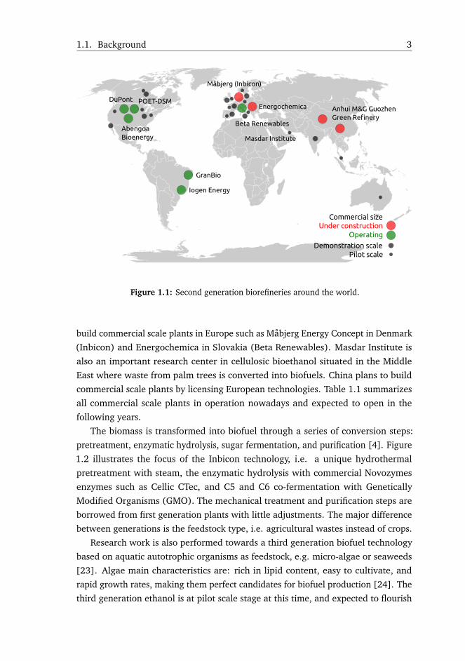
1.1. Background 3
Figure 1.1: Second generation biorefineries around the world.
build commercial scale plants in Europe such as Måbjerg Energy Concept in Denmark
(Inbicon) and Energochemica in Slovakia (Beta Renewables). Masdar Institute is
also an important research center in cellulosic bioethanol situated in the Middle
East where waste from palm trees is converted into biofuels. China plans to build
commercial scale plants by licensing European technologies. Table 1.1 summarizes
all commercial scale plants in operation nowadays and expected to open in the
following years.
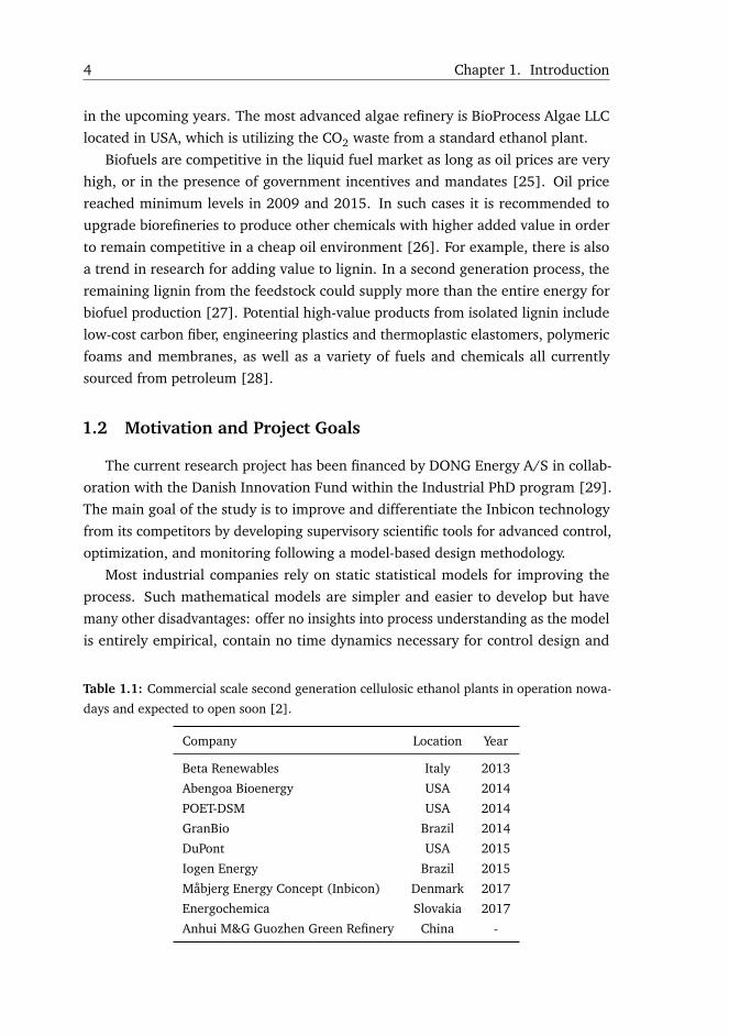
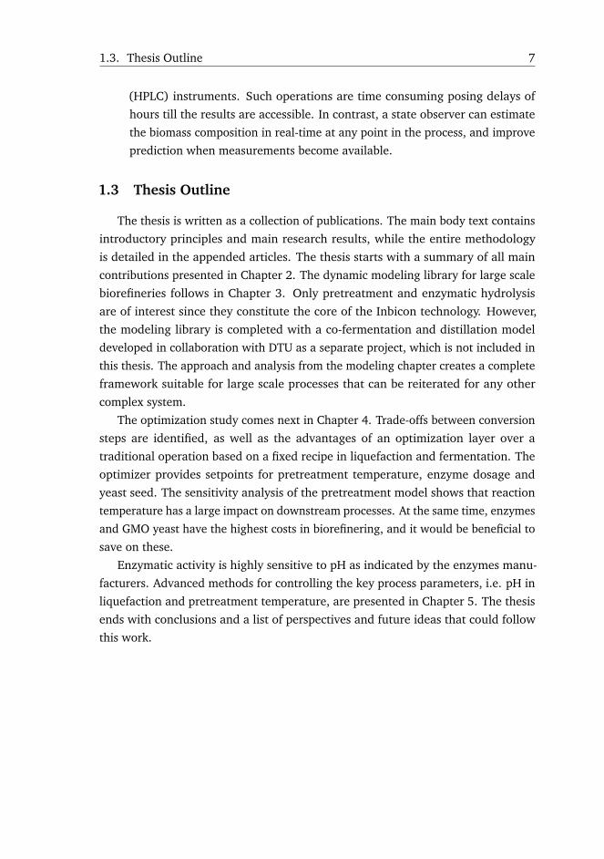
The biomass is transformed into biofuel through a series of conversion steps:
pretreatment, enzymatic hydrolysis, sugar fermentation, and purification [4]. Figure
1.2 illustrates the focus of the Inbicon technology, i.e. a unique hydrothermal
pretreatment with steam, the enzymatic hydrolysis with commercial Novozymes
enzymes such as Cellic CTec, and C5 and C6 co-fermentation with Genetically
Modified Organisms (GMO). The mechanical treatment and purification steps are
borrowed from first generation plants with little adjustments. The major difference
between generations is the feedstock type, i.e. agricultural wastes instead of crops.
Research work is also performed towards a third generation biofuel technology
based on aquatic autotrophic organisms as feedstock, e.g. micro-algae or seaweeds
[23]. Algae main characteristics are: rich in lipid content, easy to cultivate, and
rapid growth rates, making them perfect candidates for biofuel production [24]. The
third generation ethanol is at pilot scale stage at this time, and expected to flourish
4 Chapter 1. Introduction
in the upcoming years. The most advanced algae refinery is BioProcess Algae LLC
located in USA, which is utilizing the CO2 waste from a standard ethanol plant.
Biofuels are competitive in the liquid fuel market as long as oil prices are very
high, or in the presence of government incentives and mandates [25]. Oil price
reached minimum levels in 2009 and 2015. In such cases it is recommended to
upgrade biorefineries to produce other chemicals with higher added value in order
to remain competitive in a cheap oil environment [26]. For example, there is also
a trend in research for adding value to lignin. In a second generation process, the
remaining lignin from the feedstock could supply more than the entire energy for
biofuel production [27]. Potential high-value products from isolated lignin include
low-cost carbon fiber, engineering plastics and thermoplastic elastomers, polymeric
foams and membranes, as well as a variety of fuels and chemicals all currently
sourced from petroleum [28].
1.2 Motivation and Project Goals
The current research project has been financed by DONG Energy A/S in collab-
oration with the Danish Innovation Fund within the Industrial PhD program [29].
The main goal of the study is to improve and differentiate the Inbicon technology
from its competitors by developing supervisory scientific tools for advanced control,
optimization, and monitoring following a model-based design methodology.
Most industrial companies rely on static statistical models for improving the
process. Such mathematical models are simpler and easier to develop but have
many other disadvantages: offer no insights into process understanding as the model
is entirely empirical, contain no time dynamics necessary for control design and
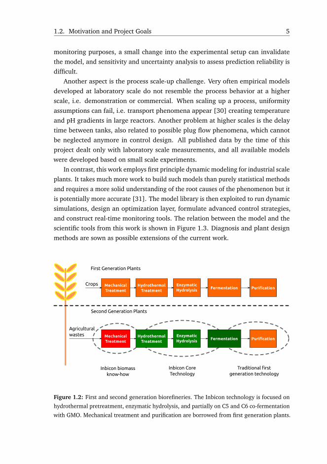
Table 1.1: Commercial scale second generation cellulosic ethanol plants in operation nowa-
days and expected to open soon [2].
Company Location Year
Beta Renewables Italy 2013
Abengoa Bioenergy USA 2014
POET-DSM USA 2014
GranBio Brazil 2014
DuPont USA 2015
Iogen Energy Brazil 2015
Måbjerg Energy Concept (Inbicon) Denmark 2017
Energochemica Slovakia 2017
Anhui M&G Guozhen Green Refinery China -
1.2. Motivation and Project Goals 5
monitoring purposes, a small change into the experimental setup can invalidate
the model, and sensitivity and uncertainty analysis to assess prediction reliability is
difficult.
Another aspect is the process scale-up challenge. Very often empirical models
developed at laboratory scale do not resemble the process behavior at a higher
scale, i.e. demonstration or commercial. When scaling up a process, uniformity
assumptions can fail, i.e. transport phenomena appear [30] creating temperature
and pH gradients in large reactors. Another problem at higher scales is the delay
time between tanks, also related to possible plug flow phenomena, which cannot
be neglected anymore in control design. All published data by the time of this
project dealt only with laboratory scale measurements, and all available models
were developed based on small scale experiments.
In contrast, this work employs first principle dynamic modeling for industrial scale
plants. It takes much more work to build such models than purely statistical methods
and requires a more solid understanding of the root causes of the phenomenon but it
is potentially more accurate [31]. The model library is then exploited to run dynamic
simulations, design an optimization layer, formulate advanced control strategies,
and construct real-time monitoring tools. The relation between the model and the
scientific tools from this work is shown in Figure 1.3. Diagnosis and plant design
methods are sown as possible extensions of the current work.
Figure 1.2: First and second generation biorefineries. The Inbicon technology is focused on
hydrothermal pretreatment, enzymatic hydrolysis, and partially on C5 and C6 co-fermentation
with GMO. Mechanical treatment and purification are borrowed from first generation plants.

6 Chapter 1. Introduction
DynamicModel
PlantSimulator
So�Sensors
Optimization
ControlDesign
DiagnosisPlantDesign
Figure 1.3: Dynamic modeling at the core of model-based scientific tools.
The specific goals of this research are:
1. To build a dynamic modeling library for pretreatment, enzymatic hydrolysis
and fermentation. The library is designed to be modular in order to allow
the user to change the configuration or add various components to the plant
architecture. The models are validated against real data extracted from the
Inbicon demonstration scale plant, and their reliability is assessed through a
comprehensive sensitivity and uncertainty analysis.
2. To analyze the biorefinery in an integrated manner for establishing an overall
optimal operation. The bioethanol production process consists of several sub-
processes. Most studies analyze and optimize each conversion step individually
in a decoupled manner without taking into account the trade-offs between
stages. Most often the found optimal operation is in fact sub-optimal when
comparing to the optimal point of an integrated system.
3. To explore the dynamic nature of the model to allow improved control design:
the low level closed loop controls could be better tuned, or more advanced
controllers such as model predictive and optimal control could be added to the
overall plant automation layout. The objective is that this would be achieved
in a simulation environment before real implementation.
4. To exploit the model to construct soft-sensors and state estimators for mon-
itoring variables of interest that are difficult to obtain in real-time in reality.
Biomass composition is measured in laboratory based on sample extractions
either with Near Infrared (NIR) or High-Performance Liquid Chromatography
1.3. Thesis Outline 7
(HPLC) instruments. Such operations are time consuming posing delays of
hours till the results are accessible. In contrast, a state observer can estimate
the biomass composition in real-time at any point in the process, and improve
prediction when measurements become available.
1.3 Thesis Outline
The thesis is written as a collection of publications. The main body text contains
introductory principles and main research results, while the entire methodology
is detailed in the appended articles. The thesis starts with a summary of all main
contributions presented in Chapter 2. The dynamic modeling library for large scale
biorefineries follows in Chapter 3. Only pretreatment and enzymatic hydrolysis
are of interest since they constitute the core of the Inbicon technology. However,
the modeling library is completed with a co-fermentation and distillation model
developed in collaboration with DTU as a separate project, which is not included in
this thesis. The approach and analysis from the modeling chapter creates a complete
framework suitable for large scale processes that can be reiterated for any other
complex system.
The optimization study comes next in Chapter 4. Trade-offs between conversion
steps are identified, as well as the advantages of an optimization layer over a
traditional operation based on a fixed recipe in liquefaction and fermentation. The
optimizer provides setpoints for pretreatment temperature, enzyme dosage and
yeast seed. The sensitivity analysis of the pretreatment model shows that reaction
temperature has a large impact on downstream processes. At the same time, enzymes
and GMO yeast have the highest costs in biorefinering, and it would be beneficial to
save on these.
Enzymatic activity is highly sensitive to pH as indicated by the enzymes manu-
facturers. Advanced methods for controlling the key process parameters, i.e. pH in
liquefaction and pretreatment temperature, are presented in Chapter 5. The thesis
ends with conclusions and a list of perspectives and future ideas that could follow
this work.

Chapter 2
Summary of Main Contributions
Journal Articles
The contributions of this research related to the modeling library and the opti-
mization layer have been published (at the time of thesis submission, the optimiza-
tion paper was undergoing the peer-review process) in three journal articles that
were included in this thesis as appendices A, B and C:
(A) R. M. Prunescu, M. Blanke, J. G. Jakobsen, and G. Sin. “Dynamic modeling and
validation of a biomass hydrothermal pretreatment process - A demonstration
scale study”. AIChE Journal (2015). DOI: 10.1002/aic.14954.
This study publishes for the first time a dynamic model for hydrothermal
pretreatment with steam that is validated against demonstration scale real
measurements. The model embeds mass and energy balances together with
computational fluid dynamics for describing a large scale thermal reactor for
biomass pretreatment. A comprehensive model analysis follows for assessing
its sensitivity and uncertainty with respect to both feed and kinetic parameters.
The dynamic trends of the process are well captured making the model suitable
for developing advanced control and monitoring strategies for large scale
plants. As an application of the model, the study includes the development of a
state observer for estimating biomass components that are difficult to measure
in reality.
(B) R. M. Prunescu and G. Sin. “Dynamic modeling and validation of a lignocellu-
losic enzymatic hydrolysis process - A demonstration scale study”. BioresourceTechnology 150 (Dec. 2013), pp. 393–403. DOI: 10.1016/j.biortech.2013.
10.029.
10 Chapter 2. Summary of Main Contributions
This work formulates a complex dynamic model for enzymatic hydrolysis of
cellulosic and hemicellulosic fibers suitable for large scale liquefaction reactors.
The model includes a competitive conversion scheme for sugar production
that was extended from previous works with hemicellulose hydrolysis, pH
and viscosity calculators, and pH dependency on reaction kinetics. For the
first time, model predictions are compared against demonstration scale real
data extracted from the Inbicon plant. A sensitivity and uncertainty analysis is
also performed to study modeling bottlenecks and for identifying the sensitive
variables that affect most the uncertainty of model predictions.
(C) R. M. Prunescu, M. Blanke, J. G. Jakobsen, and G. Sin. “Model-Based Plantwide
Optimization of a Large Scale Lignocellulosic Bioethanol Plant”. Submitted toAIChE Journal (2015).
The scientific novelty of this work is the design of a plantwide model-based
optimization layer for a large scale biorefinery. The objective is to maximize
the economic profit by searching for the best trade-off between the conversion
steps. The optimization solver can be triggered whenever there is a change
in prices or feedstock composition, adapting the plant to market and oper-
ation conditions in order to maximize profitability at any given time. The
optimization layer undergoes a sensitivity and uncertainty analysis for finding
the variables that affect most the optimal point, and hence the economical
profit. It is found that the optimization strategy is capable of reducing the
uncertainty on the profit curve when compared to a traditional operation, and
also allows running the plant in a wider nominal range with small impact on
profitability. Feedstock composition impacts more on profit than model kinetics
showing the need of accurate measurements of its composition.
Peer Reviewed Conference Proceedings (Web of Science)
The results concerning the advanced adaptive control strategies for process key
parameters were disseminated in two peer-reviewed IEEE conference papers that
were included in this thesis as appendices D and E:
(D) R. M. Prunescu, M. Blanke, and G. Sin. “Modelling and L1 Adaptive Control of
Temperature in Biomass Pretreatment”. Proceedings of the 52nd IEEE Conferenceon Decision and Control. Florence, Italy, 2013, pp. 3152–3159.
It has been shown in the sensitivity analysis of the pretreatment process that
thermal conditions impact all downstream processes. Maintaining a steady
reaction temperature, as well as quick reference tracking as imposed by the
11
optimization layer is of interest in this study. The main contribution refers to
the application of an L1 adaptive output feedback controller for this type of
process. The tuning method is also new consisting of numerical optimization
for minimizing the Integral Absolute Error (IAE) cost function with respect to
the controller parameters.
(E) R. M. Prunescu, M. Blanke, and G. Sin. “Modelling and L1 Adaptive Control
of pH in Bioethanol Enzymatic Process”. Proceedings of the 2013 AmericanControl Conference. Washington D.C., USA, 2013, pp. 1888–1895.
Enzymatic activity is sensitive to the pH of the medium. The titration curve is
highly nonlinear and poses a difficult challenge for any control strategy. The
contribution from this work refers to the application of an L1 adaptive output
feedback controller for enzymatic pH. The tuning method is new for this kind
of processes, and relies on closed loop transfer function analysis that takes into
account the interactions between the output predictor, the control signal filter
and adaptation law.
Unpublished Work
There are two unpublished contributions included in this thesis:
(Section 3.4.4) A fast pH calculator with guaranteed accuracy for dynamic simu-
lations:
pH is a key process parameter both in enzymatic hydrolysis
and fermentation. The novelty from this section refers to a pH
calculator that converges in a known amount of steps depend-
ing on the demanded accuracy. The algorithm is based on the
charge balance of the liquid phase, and uses a modified bisection
method that advances in logarithmic space for finding the pH
level. The dynamic nature of simulations is also exploited, taking
into account the solution from the previous simulation step in
order to find tight bounds around the possible solution. The pH
calculator has proven to be reliable and fast with guaranteed
accuracy.
(Section 5.4) An optimal controller for the feed profile in glucose fermenta-
tion:
Fermentation reactors have a large volume and it can take days
to fill the tanks till the desired hold-up, time when reactions

12 Chapter 2. Summary of Main Contributions
already take place. The contribution from this section shows
how to compute an optimal feed rate profile such that inhibitors
accumulation is avoided and yeast seed is minimized. The profile
is found by formulating an Optimal Control Problem (OCP) and
then compared to a classical constant feed strategy. The greatest
benefit of a variable feed rate is that yeast amount is significantly
reduced contributing to lower costs in fermentation.
Conference Presentations
All contributions were also disseminated in prestigious conferences through
specialized session talks:
• R. M. Prunescu, M. Blanke, J. G. Jakobsen, and G. Sin. “Dynamic Modeling,
Advanced Control, Diagnosis and Optimization of Large-Scale Lignocellulosic
Biorefineries”. Proceedings of the AIChE 2015 Annual Meeting. Salt Lake City,
UT, USA, 2015.
• R. M. Prunescu, M. Blanke, J. G. Jakobsen, and G. Sin. “Plantwide Model-Based
Optimization of a Large Scale Second Generation Biorefinery”. Proceedings ofthe AIChE 2015 Annual Meeting. Salt Lake City, UT, USA, 2015.
• R. M. Prunescu, M. Blanke, J. G. Jakobsen, and G. Sin. “Model-Based Filtering
of Large-Scale Datasets - A Biorefinery Application”. Proceedings of the AIChE2014 Annual Meeting. Atlanta, GA, USA, 2014.
• R. M. Prunescu and G. Sin. “Dynamic Simulation, Sensitivity and Uncer-
tainty Analysis of a Demonstration Scale Lignocellulosic Enzymatic Hydrolysis
Process”. Proceedings of the AIChE 2014 Annual Meeting. Atlanta, GA, USA,
2014.
• R. M. Prunescu, M. Blanke, and G. Sin. “Advances in Monitoring, Diagnosis
and Control of Biorefineries”. Proceedings of the 9th World Congress of ChemicalEngineering. Seoul, South Korea, 2013.
Chapter 3
Dynamic Modeling and Analysis
3.1 Introduction
This chapter presents the main results from two scientific journal publications
included in appendix as Paper A and Paper B. The focus is placed on biomass
pretreatment and enzymatic hydrolysis, which are the core processes of the Inbicon
technology. The co-fermentation model constitutes the subject of a separate project,
while the purification technology is state of the art with no customization for Inbicon.
Therefore the liquefaction and distillation processes are not included in this work.
The chapter starts with a detailed description of the Inbicon second generation
bioethanol plant, followed by the model analysis methodology. The entire mathe-
matical model library is then summarized, and the main sensitivity and uncertainty
analysis results are discussed. The chapter ends with conclusions and suggestions
for future modeling improvements and maintenance.
3.2 Process Description
This section describes the composition of feedstock used in second generation
biorefineries including technical details for each biomass conversion step, i.e. pre-
treatment, enzymatic hydrolysis, co-fermentation and purification.
3.2.1 Biomass Characterization
Lignocellulosic biomass consists of cellulose, hemicellulose, lignin, ash, and
other residues in negligible amounts [37]. Hemicellulose further divides into xylan,
arabinan, galactan, mannan and acetyl groups [38]. Table 3.1 shows different
biomass compositions depending on agricultural waste type, e.g. bagasse, wheat
straw, miscanthus, corn stover, or quinoa stalks. Even if the biomass is of the same

14 Chapter 3. Dynamic Modeling and Analysis
type, it can still have a different percentage distribution of its components due to
seasonality, harvest location, amount of rain, or used fertilizers for growing the crops.
The solid composition of biomass is typically measured with NIR instruments based
on laboratory samples, and is essential for determining the biofuel potential for each
biomass type [39]. The feedstock has an initial dry matter of over 85 %.
Table 3.1: Composition of different raw biomass types in percentage of dry matter. Some
components were not measured (n/m).
Biomass Cellulose Xylan Arabinan Lignin Ash Acetyls Other Reference
Wheat straw 39.8 24.5 2.8 22.6 4.2 n/m 6.1 [40]
Wheat straw 42.1 23.4 1.9 21.6 2.1 n/m 8.9 [41]
Corn stover 35.0 18.5 n/m 13.9 3.8 3.2 25.6 [42]
Corn stover 34.0 19.2 2.5 12.3 4.7 2.9 24.4 [43]
Bagasse 39.0 21.8 1.8 24.8 3.9 3.3 5.4 [43]
Miscanthus 38.2 20.9 1.5 26.4 2.6 4.1 6.3 [44]
Quinoa stalks 35.7 15.4 3.5 21.9 4.2 2.7 16.6 [38]
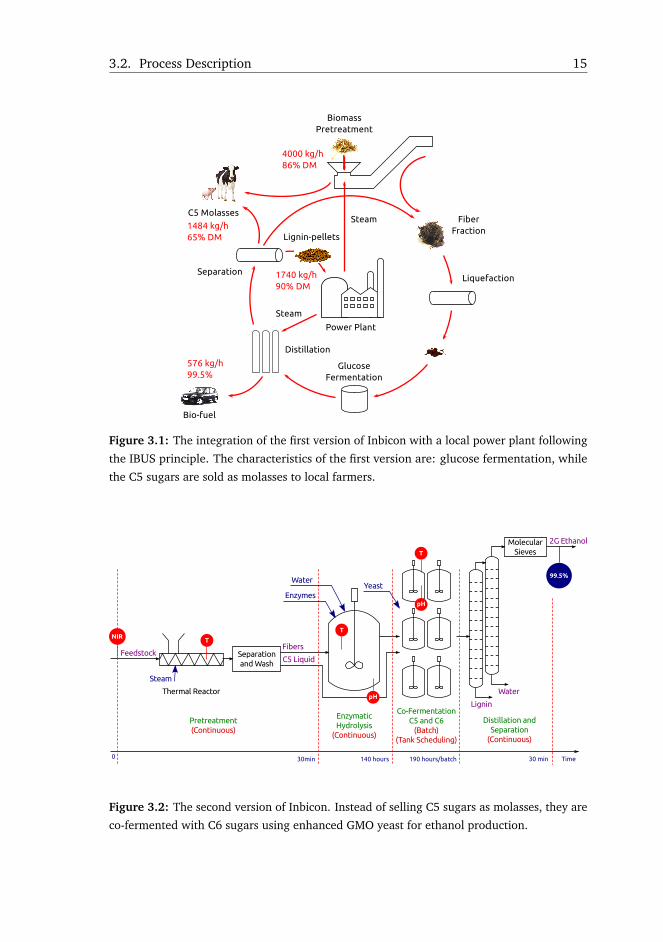
3.2.2 The Inbicon Biorefinery
The Inbicon biorefinery is integrated with Asnæs power plant (also owned by
DONG Energy A/S) following the IBUS principle [4]. The symbiosis between
the refinery and the plant is illustrated in Figure 3.1. The biorefinery receives
steam at 18 bar for a low cost, and returns lignin-pellets to be co-burnt with coal
in the power plant for steam and power generation. The steam fuels the biomass
pretreatment and purification processes. Figure 3.1 illustrates the first version of
Inbicon where the C5 sugars from the pretreatment process were transformed into
molasses along with wasted yeast from fermentation, and sold to local farmers to
feed their cattle. The conversion steps are: pretreatment, enzymatic hydrolysis
or liquefaction, fermentation, and purification. Bioethanol is the main refined
product, followed by two other by-products, i.e. C5 molasses and lignin-pellets. The
first version of the Inbicon demonstration scale plant produces 576 kg of biofuel,
1484 kg of molasses, and 1740 kg of lignin-pellets from 4 t of dry biomass, which is
the nominal throughput per hour of the plant [3]. The amount of lignin-pellets
generates enough energy to cover the requirements for biofuel production [27].
The second version of Inbicon is shown in Figure 3.2. The C5 sugars are no
longer transformed into molasses but rather used in co-fermentation with GMO
yeast. The stream with C5 sugars by-passes the enzymatic hydrolysis tanks and is
directed to fermentation. Results show that the latest Inbicon version increases the
3.2. Process Description 15
Figure 3.1: The integration of the first version of Inbicon with a local power plant following
the IBUS principle. The characteristics of the first version are: glucose fermentation, while
the C5 sugars are sold as molasses to local farmers.
Figure 3.2: The second version of Inbicon. Instead of selling C5 sugars as molasses, they are
co-fermented with C6 sugars using enhanced GMO yeast for ethanol production.
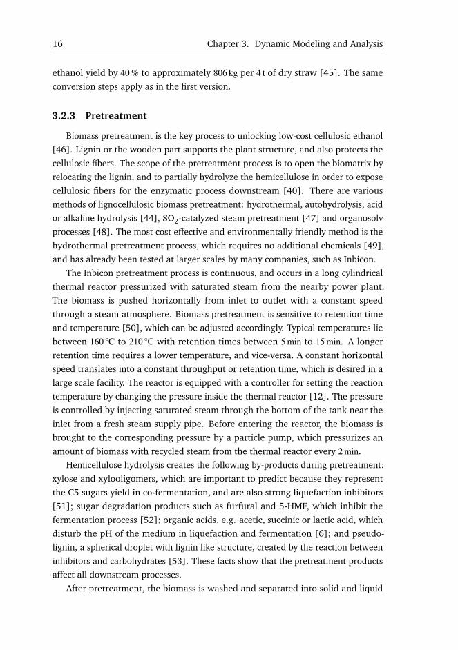
16 Chapter 3. Dynamic Modeling and Analysis
ethanol yield by 40 % to approximately 806 kg per 4 t of dry straw [45]. The same
conversion steps apply as in the first version.
3.2.3 Pretreatment
Biomass pretreatment is the key process to unlocking low-cost cellulosic ethanol
[46]. Lignin or the wooden part supports the plant structure, and also protects the
cellulosic fibers. The scope of the pretreatment process is to open the biomatrix by
relocating the lignin, and to partially hydrolyze the hemicellulose in order to expose
cellulosic fibers for the enzymatic process downstream [40]. There are various
methods of lignocellulosic biomass pretreatment: hydrothermal, autohydrolysis, acid
or alkaline hydrolysis [44], SO2-catalyzed steam pretreatment [47] and organosolv
processes [48]. The most cost effective and environmentally friendly method is the
hydrothermal pretreatment process, which requires no additional chemicals [49],
and has already been tested at larger scales by many companies, such as Inbicon.
The Inbicon pretreatment process is continuous, and occurs in a long cylindrical
thermal reactor pressurized with saturated steam from the nearby power plant.
The biomass is pushed horizontally from inlet to outlet with a constant speed
through a steam atmosphere. Biomass pretreatment is sensitive to retention time
and temperature [50], which can be adjusted accordingly. Typical temperatures lie
between 160 ◦C to 210 ◦C with retention times between 5 min to 15 min. A longer
retention time requires a lower temperature, and vice-versa. A constant horizontal
speed translates into a constant throughput or retention time, which is desired in a
large scale facility. The reactor is equipped with a controller for setting the reaction
temperature by changing the pressure inside the thermal reactor [12]. The pressure
is controlled by injecting saturated steam through the bottom of the tank near the
inlet from a fresh steam supply pipe. Before entering the reactor, the biomass is
brought to the corresponding pressure by a particle pump, which pressurizes an
amount of biomass with recycled steam from the thermal reactor every 2 min.
Hemicellulose hydrolysis creates the following by-products during pretreatment:
xylose and xylooligomers, which are important to predict because they represent
the C5 sugars yield in co-fermentation, and are also strong liquefaction inhibitors
[51]; sugar degradation products such as furfural and 5-HMF, which inhibit the
fermentation process [52]; organic acids, e.g. acetic, succinic or lactic acid, which
disturb the pH of the medium in liquefaction and fermentation [6]; and pseudo-
lignin, a spherical droplet with lignin like structure, created by the reaction between
inhibitors and carbohydrates [53]. These facts show that the pretreatment products
affect all downstream processes.
After pretreatment, the biomass is washed and separated into solid and liquid

3.2. Process Description 17
parts by a screw press. The solid part is rich in cellulose, while the liquid part
contains the C5 sugars that were produced due to hemicellulose hydrolysis.
3.2.4 Enzymatic Hydrolysis
A conveyor belt transports the cellulosic fibers to the enzymatic hydrolysis reactor.
The Inbicon liquefaction process is also continuous, and occurs in several reactors
connected in series. The first tank is a 5-chambers hydrolysis reactor presented
in [54] that was specifically designed for high dry matter liquefaction of biomass
preferably around 35 % [55]. There is an abrupt change in viscosity in the first hours
of hydrolysis allowing the slurry to be easily pumped afterwards. The rheology
phenomena is well documented in torque measurements, which decrease exponen-
tially [56]. The following tanks are conventional Continuous Stirred Tank Reactors
(CSTRs) linked in series to meet the necessary hydrolysis time of 140 h. There are
many commercially available enzymes, e.g. Cellic CTec2 [57], Cellic CTec3 [58],
Cellic HTec3 [59]. The hydrolysis retention time can be adjusted either by changing
the tank hold-ups (preferably) or by setting a different refinery throughput.
Nowadays enzymes are capable of hydrolyzing both cellulosic and hemicellulosic
fibers. Cellulose hydrolysis produces glucose with cellobiose intermediate product,
while hemicellulose hydrolysis is more complex leading to xylooligomers, xylose
and organic acids production. The enzymatic mixture is a cocktail of cellulase and
xylanase. Cellulase hydrolyzes cellulose, and consists of exo-β -1.4-cellobiohydrolase,
endo-β -1.4-glucanase, and β -glucosidase [60]. Cellulose is a long solid polymer
or chain made up of glucose units. The endo-β -1.4-glucanase randomly breaks
internal bonds from the cellulosic fibers creating new chain ends. The exo-β -1.4-
cellobiohydrolases further cleave the endo-glucanase products producing cellobiose.
The β -glucosidase enzymes breaks cellobiose into glucose. The xylanase enzymes
behave similarly with xylooligomers intermediate product but along with hemicellu-
lose hydrolysis it also releases acetyls, which produces acetic acid affecting the pH
of the medium in the reactor.
The enzymatic activity is sensitive to pH and temperature following a bell shaped
efficiency curve with a single peak [11]. Temperature control is easily achieved,
while pH control has many challenges due to the nonlinearities in the titration curve
[11]. All enzymatic hydrolysis reactors have temperature and pH controllers. The
degree of biomatrix opening or treatment severity, and some pretreatment inhibitors,
i.e. xylooligomers and xylose, reduces the enzymatic activity. Also, liquefaction is a
competitive mechanism with product inhibition. Enzymes can be inhibited but also
irreversibly deactivated in time and due to wrong temperature exposure [61].
18 Chapter 3. Dynamic Modeling and Analysis
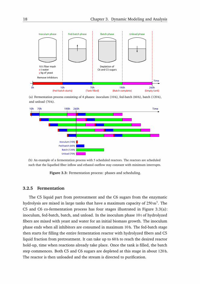
(a) Fermentation process consisting of 4 phases: inoculum (10 h), fed-batch (60 h), batch (120 h),and unload (70 h).
(b) An example of a fermentation process with 5 scheduled reactors. The reactors are scheduledsuch that the liquefied fiber inflow and ethanol outflow stay constant with minimum interrupts.
Figure 3.3: Fermentation process: phases and scheduling.
3.2.5 Fermentation
The C5 liquid part from pretreatment and the C6 sugars from the enzymatic
hydrolysis are mixed in large tanks that have a maximum capacity of 250 m3. The
C5 and C6 co-fermentation process has four stages illustrated in Figure 3.3(a):
inoculum, fed-batch, batch, and unload. In the inoculum phase 10 t of hydrolyzed
fibers are mixed with yeast and water for an initial biomass growth. The inoculum
phase ends when all inhibitors are consumed in maximum 10 h. The fed-batch stage
then starts for filling the entire fermentation reactor with hydrolyzed fibers and C5
liquid fraction from pretreatment. It can take up to 60 h to reach the desired reactor
hold-up, time when reactions already take place. Once the tank is filled, the batch
step commences. Both C5 and C6 sugars are depleted at this stage in about 120 h.
The reactor is then unloaded and the stream is directed to purification.
3.3. Model Analysis Framework 19
The fermenters have temperature and pH controllers. Typical operation condi-
tions are 35 ◦C and 5.5 pH units, which are optimal for the GMO yeast. The enzymes
are still active during fermentation making the system a simultaneous saccharifi-
cation and fermentation process. The liquefied fibers still contain solid cellulose
and hemicellulose that were not entirely hydrolyzed during liquefaction because of
product inhibition. As sugars are depleted in fermentation for ethanol production,
the sugars inhibitory effect decreases, and enzymes continue the liquefaction process
simultaneously.
In large scale facilities, fermentation runs in a batch manner requiring more
reactors to run in parallel according to a scheduling algorithm as illustrated in
Figure 3.3(b). The operation is aligned such that input and output streams flow
continuously with minimum interruptions.
3.2.6 Purification
The first distillation column separates lignin from the stream. The lignin is sent to
a local evaporation unit, which creates the lignin bio-pellets. The second distillation
column purifies ethanol further, which reaches 99.5 % purity after the molecular
sieves. The bioethanol is stored in underground tanks till an oil company transports
them to their facilities to be blended with regular gasoline. The bioethanol is sold at
petrol stations as E10, E15, E20, or E85, the number indicating the percentage of
ethanol from the mix, e.g. E10 contains 10 % bioethanol and 90 % gasoline.
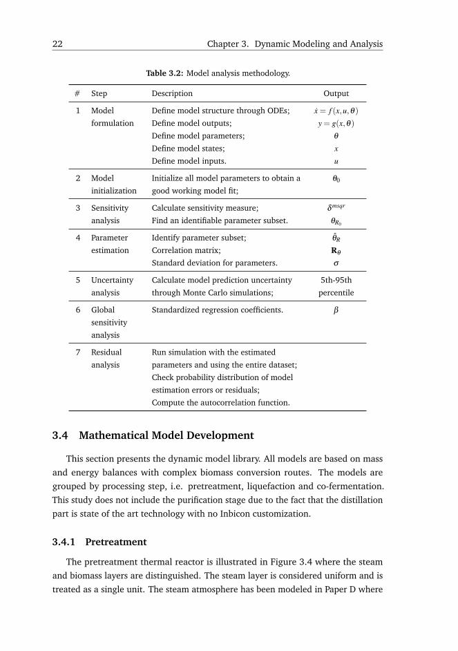
3.3 Model Analysis Framework
The model analysis framework is summarized in Table 3.2, which is detailed in
the next 7 steps:
1. Formulate the mathematical model structure as a system of nonlinear Ordinary
Differential Equations (ODEs). Identify states, inputs, outputs and model
parameters:x = f (x,u,θ)y = g(x,θ)
(3.1)
f is an array of nonlinear functions of states x, inputs u, and parameters θ . The
outputs y are defined as nonlinear functions g of states x and model parameters
θ .
2. The second step is to calibrate the model considering the entire set of param-
eters. This system identification exercise follows the nonlinear least squares
method for grey-box models, which should give the set of parameters that has
20 Chapter 3. Dynamic Modeling and Analysis
the smallest sum of squared errors between model predicted output and actual
measurements [62]:
minθ
N
∑i=1
e2i (3.2)
ei is the estimation error at sample time i defined as ei = yi − yi, the real
measurement yi and the predicted output yi. In the present case, this is a
nonlinear least squares problem and local minima can be obstacles.
3. The third step is to investigate which model parameters could be identified
given the input and the model structure [63]. This selection is achieved
through assessment of sensitivity of the partial derivatives of the cost function
with respect to each model parameter. The delta mean square δ msqrik defined by
[64] is a measure of sensitivity suitable for time varying signals:
δ msqrik =
√1N
s>nd,iksnd,ik (3.3)
where k is the parameter index, i is the model output index, N is the number of
samples, and snd,ik is a vector with the non dimensional sensitivity calculated
in each sample:
snd,ik =∂yi
∂θk
θk
sci(3.4)
∂yi/∂θk represents the output variation with respect to parameter θk, and sci
is a scaling factor with the same physical dimension as the corresponding
observation in order to make this measure non dimensional. In this study, the
scaling factor is chosen as the mean value of output i:
sci =1N
N
∑1
yi(k) (3.5)
After computing the sensitivities δ msqr, all parameters are ranked with respect
to their value of δ msqr. Parameters that have low sensitivity are more uncertain
than those with high sensitivity and would not contribute to model accuracy.
In case of systems with multiple outputs, a cumulative sensitivity measure is
defined as:
δ msqrk =
ny
∑i=1
δ msqrik (3.6)
The relevant subset of parameters is selected based on δ msqr being higher than
a threshold.
4. The reduced set of parameters is properly estimated following the same min-
imization technique from step 2. In this case, the real measurements are
3.3. Model Analysis Framework 21
in fact NIR or HPLC laboratory datasets from the demonstration plant. The
whole dataset is split into estimation and validation subsets. The parameter
estimation procedure runs on the estimation dataset. The correlation matrix
and standard deviations of the estimates are also calculated.
5. This step quantifies the prediction uncertainty. Having the covariance matrix
and standard deviations from the previous step allows LHS with correlation
control [65]. The feed parameters is another source of uncertainty and is
included in this analysis. Monte Carlo simulations are then run with sampled
parameter values and the 5th-50th-95th percentiles of the model predictions
are found.
6. A global sensitivity analysis follows by fitting a linear model from parameters
to model predictions from the Monte Carlo simulations [66, 67]:
yregi = a+∑k
bkθk (3.7)
where yregi is the ith output, and a and bk are the linear model parameters. The
standardized regression coefficients β are a global sensitivity measure, and are
defined as:
βk =σθRk
σyi
bk (3.8)
where βk is the β coefficient, σθRkis the standard deviation of the parameter
estimate, σyi is the standard deviation of output i, and bk is the linear model pa-
rameter. βk is an indicator for how much the parameter uncertainty contributes
to the prediction uncertainty.
7. The model estimation error or the residuals are analyzed in this step. A simu-
lation is run with the estimated parameters using the entire set of data (both
validation and estimation sets). The residuals distribution and autocorrelation
are calculated in order to assess the quality of model predictions. A good
model captures most of the signal in measurements and is characterized by
residuals being Gaussian with uncorrelated increments.
The sensitivity and uncertainty analysis based on Monte Carlo simulations has
been successfully applied in numerous situations, e.g. in enzymatic biodiesel pro-
duction [68], cellulose hydrolysis [8], wastewater plant treatment [66], or lignocel-
lulosic ethanol plants [9].
22 Chapter 3. Dynamic Modeling and Analysis
Table 3.2: Model analysis methodology.
# Step Description Output
1 Model
formulation
Define model structure through ODEs; x = f (x,u,θ)Define model outputs; y = g(x,θ)Define model parameters; θDefine model states; x
Define model inputs. u
2 Model
initialization
Initialize all model parameters to obtain a
good working model fit;
θ0
3 Sensitivity
analysis
Calculate sensitivity measure; δ msqr
Find an identifiable parameter subset. θR0
4 Parameter
estimation
Identify parameter subset; θR
Correlation matrix; Rθ
Standard deviation for parameters. σ
5 Uncertainty
analysis
Calculate model prediction uncertainty
through Monte Carlo simulations;
5th-95th
percentile
6 Global
sensitivity
analysis
Standardized regression coefficients. β
7 Residual
analysis
Run simulation with the estimated
parameters and using the entire dataset;
Check probability distribution of model
estimation errors or residuals;
Compute the autocorrelation function.
3.4 Mathematical Model Development
This section presents the dynamic model library. All models are based on mass
and energy balances with complex biomass conversion routes. The models are
grouped by processing step, i.e. pretreatment, liquefaction and co-fermentation.
This study does not include the purification stage due to the fact that the distillation
part is state of the art technology with no Inbicon customization.
3.4.1 Pretreatment
The pretreatment thermal reactor is illustrated in Figure 3.4 where the steam
and biomass layers are distinguished. The steam layer is considered uniform and is
treated as a single unit. The steam atmosphere has been modeled in Paper D where
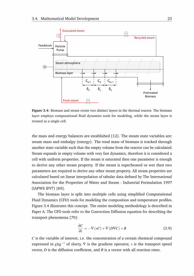
3.4. Mathematical Model Development 23
Figure 3.4: Biomass and steam create two distinct layers in the thermal reactor. The biomass
layer employs computational fluid dynamics tools for modeling, while the steam layer is
treated as a single cell.
the mass and energy balances are established [12]. The steam state variables are:
steam mass and enthalpy (energy). The total mass of biomass is tracked through
another state variable such that the empty volume from the reactor can be calculated.
Steam expands in empty volume with very fast dynamics, therefore it is considered a
cell with uniform properties. If the steam is saturated then one parameter is enough
to derive any other steam property. If the steam is superheated or wet then two
parameters are required to derive any other steam property. All steam properties are
calculated based on linear interpolation of tabular data defined by The International
Association for the Properties of Water and Steam - Industrial Formulation 1997
(IAPWS IF97) [69].
The biomass layer is split into multiple cells using simplified Computational
Fluid Dynamics (CFD) tools for modeling the composition and temperature profiles.
Figure 3.4 illustrates this concept. The entire modeling methodology is described in
Paper A. The CFD tools refer to the Convection Diffusion equation for describing the
transport phenomena [70]:
∂C∂ t
=−∇(vC)+∇(D∇C)+R (3.9)
C is the variable of interest, i.e. the concentration of a certain chemical compound
expressed in gkg−1 of slurry, ∇ is the gradient operator, v is the transport speed
vector, D is the diffusion coefficient, and R is a vector with all reaction rates.
24 Chapter 3. Dynamic Modeling and Analysis
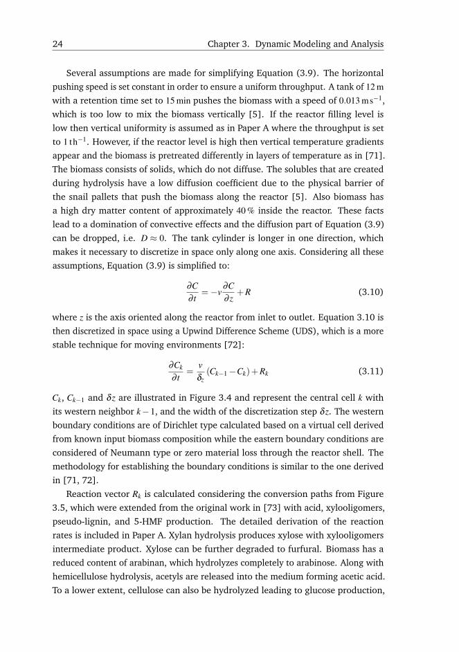
Several assumptions are made for simplifying Equation (3.9). The horizontal
pushing speed is set constant in order to ensure a uniform throughput. A tank of 12 mwith a retention time set to 15 min pushes the biomass with a speed of 0.013 ms−1,
which is too low to mix the biomass vertically [5]. If the reactor filling level is
low then vertical uniformity is assumed as in Paper A where the throughput is set
to 1 th−1. However, if the reactor level is high then vertical temperature gradients
appear and the biomass is pretreated differently in layers of temperature as in [71].
The biomass consists of solids, which do not diffuse. The solubles that are created
during hydrolysis have a low diffusion coefficient due to the physical barrier of
the snail pallets that push the biomass along the reactor [5]. Also biomass has
a high dry matter content of approximately 40 % inside the reactor. These facts
lead to a domination of convective effects and the diffusion part of Equation (3.9)
can be dropped, i.e. D ≈ 0. The tank cylinder is longer in one direction, which
makes it necessary to discretize in space only along one axis. Considering all these
assumptions, Equation (3.9) is simplified to:
∂C∂ t
=−v∂C∂ z
+R (3.10)
where z is the axis oriented along the reactor from inlet to outlet. Equation 3.10 is
then discretized in space using a Upwind Difference Scheme (UDS), which is a more
stable technique for moving environments [72]:
∂Ck
∂ t=
vδz
(Ck−1−Ck)+Rk (3.11)
Ck, Ck−1 and δ z are illustrated in Figure 3.4 and represent the central cell k with
its western neighbor k−1, and the width of the discretization step δ z. The western
boundary conditions are of Dirichlet type calculated based on a virtual cell derived
from known input biomass composition while the eastern boundary conditions are
considered of Neumann type or zero material loss through the reactor shell. The
methodology for establishing the boundary conditions is similar to the one derived
in [71, 72].
Reaction vector Rk is calculated considering the conversion paths from Figure
3.5, which were extended from the original work in [73] with acid, xylooligomers,
pseudo-lignin, and 5-HMF production. The detailed derivation of the reaction
rates is included in Paper A. Xylan hydrolysis produces xylose with xylooligomers
intermediate product. Xylose can be further degraded to furfural. Biomass has a
reduced content of arabinan, which hydrolyzes completely to arabinose. Along with
hemicellulose hydrolysis, acetyls are released into the medium forming acetic acid.
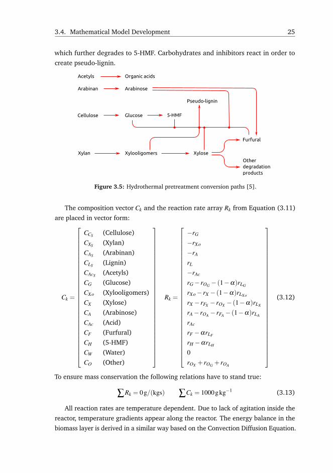
To a lower extent, cellulose can also be hydrolyzed leading to glucose production,
3.4. Mathematical Model Development 25
which further degrades to 5-HMF. Carbohydrates and inhibitors react in order to
create pseudo-lignin.
Figure 3.5: Hydrothermal pretreatment conversion paths [5].
The composition vector Ck and the reaction rate array Rk from Equation (3.11)
are placed in vector form:
Ck =
CCS (Cellulose)
CXS (Xylan)
CAS (Arabinan)
CLS (Lignin)
CAcS (Acetyls)
CG (Glucose)
CXo (Xylooligomers)
CX (Xylose)
CA (Arabinose)
CAc (Acid)
CF (Furfural)
CH (5-HMF)
CW (Water)
CO (Other)
Rk =
−rG
−rXo
−rA
rL
−rAc
rG− rOG − (1−α)rLG
rXo− rX − (1−α)rLXo
rX − rFX − rOX − (1−α)rLX
rA− rOA − rFA − (1−α)rLA
rAc
rF −αrLF
rH −αrLH
0rOX + rOG + rOA
(3.12)
To ensure mass conservation the following relations have to stand true:
∑Rk = 0g/(kgs) ∑Ck = 1000gkg−1 (3.13)
All reaction rates are temperature dependent. Due to lack of agitation inside the
reactor, temperature gradients appear along the reactor. The energy balance in the
biomass layer is derived in a similar way based on the Convection Diffusion Equation.
26 Chapter 3. Dynamic Modeling and Analysis
Biomass has insulation properties resulting in a low heat diffusion coefficient. Only
convective effects are assumed. The variable of interest in this case is the enthalpy h
expressed in kJkg−1:
∂h∂ t
=−v∂h∂ z
+Qk⇒∂hk
∂ t=
vδ z
(hk−1−hk)+Qk (3.14)
where Qk is the energy inflow in cell k. The same cell grid is used as in the biomass
composition case. The steam injection occurs near the inlet and is lumped into the
boundary conditions, which are detailed in Paper A. The temperature gradient is
then obtained by dividing the enthalpy to the specific heat.
3.4.2 Enzymatic Hydrolysis
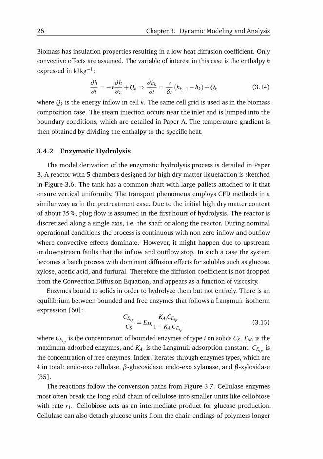
The model derivation of the enzymatic hydrolysis process is detailed in Paper
B. A reactor with 5 chambers designed for high dry matter liquefaction is sketched
in Figure 3.6. The tank has a common shaft with large pallets attached to it that
ensure vertical uniformity. The transport phenomena employs CFD methods in a
similar way as in the pretreatment case. Due to the initial high dry matter content
of about 35 %, plug flow is assumed in the first hours of hydrolysis. The reactor is
discretized along a single axis, i.e. the shaft or along the reactor. During nominal
operational conditions the process is continuous with non zero inflow and outflow
where convective effects dominate. However, it might happen due to upstream
or downstream faults that the inflow and outflow stop. In such a case the system
becomes a batch process with dominant diffusion effects for solubles such as glucose,
xylose, acetic acid, and furfural. Therefore the diffusion coefficient is not dropped
from the Convection Diffusion Equation, and appears as a function of viscosity.
Enzymes bound to solids in order to hydrolyze them but not entirely. There is an
equilibrium between bounded and free enzymes that follows a Langmuir isotherm
expression [60]:CEiB
CS= EMi
KAiCEiF
1+KAiCEiF
(3.15)
where CEiBis the concentration of bounded enzymes of type i on solids CS. EMi is the
maximum adsorbed enzymes, and KAi is the Langmuir adsorption constant. CEiFis
the concentration of free enzymes. Index i iterates through enzymes types, which are
4 in total: endo-exo cellulase, β -glucosidase, endo-exo xylanase, and β -xylosidase
[35].
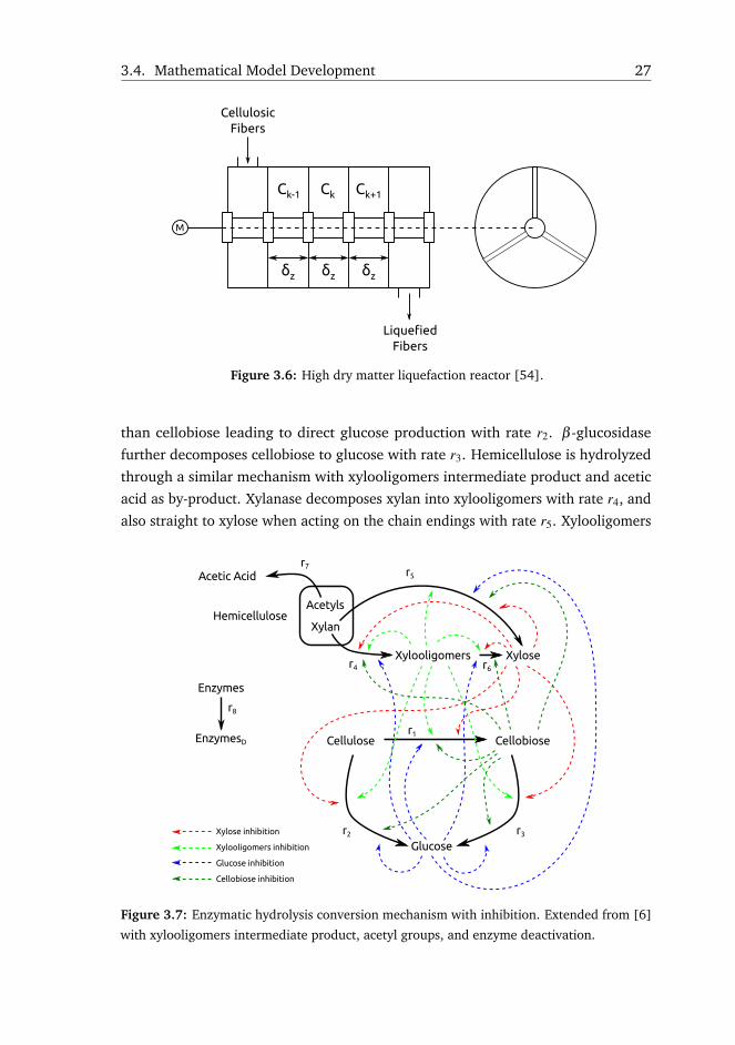
The reactions follow the conversion paths from Figure 3.7. Cellulase enzymes
most often break the long solid chain of cellulose into smaller units like cellobiose
with rate r1. Cellobiose acts as an intermediate product for glucose production.
Cellulase can also detach glucose units from the chain endings of polymers longer
3.4. Mathematical Model Development 27
Figure 3.6: High dry matter liquefaction reactor [54].
than cellobiose leading to direct glucose production with rate r2. β -glucosidase
further decomposes cellobiose to glucose with rate r3. Hemicellulose is hydrolyzed
through a similar mechanism with xylooligomers intermediate product and acetic
acid as by-product. Xylanase decomposes xylan into xylooligomers with rate r4, and
also straight to xylose when acting on the chain endings with rate r5. Xylooligomers
Figure 3.7: Enzymatic hydrolysis conversion mechanism with inhibition. Extended from [6]
with xylooligomers intermediate product, acetyl groups, and enzyme deactivation.
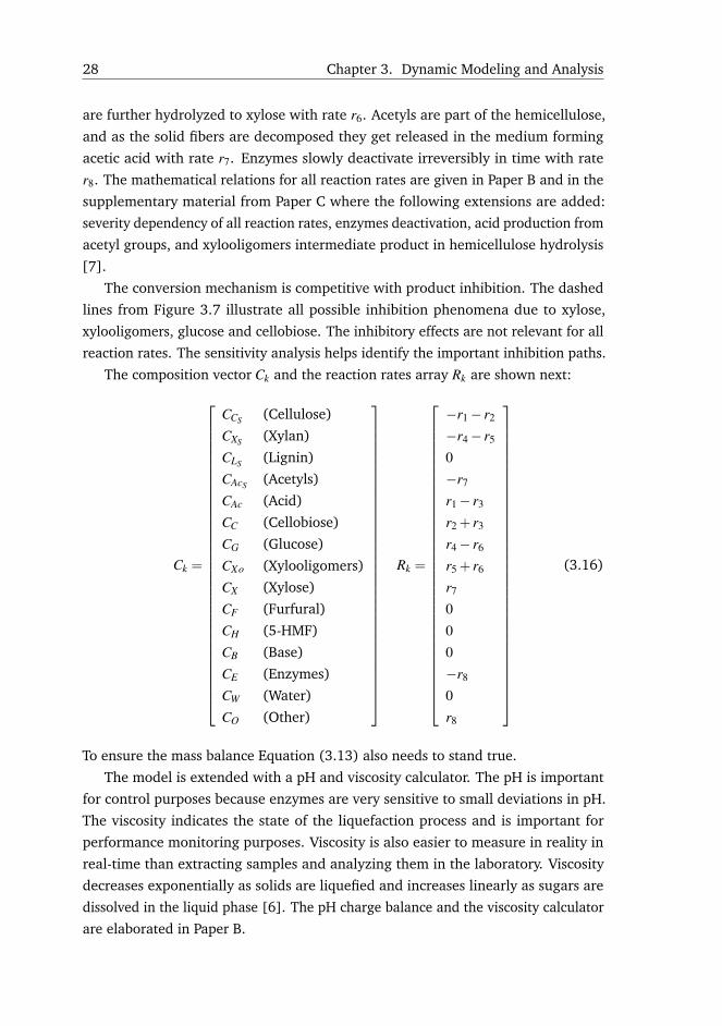
28 Chapter 3. Dynamic Modeling and Analysis
are further hydrolyzed to xylose with rate r6. Acetyls are part of the hemicellulose,
and as the solid fibers are decomposed they get released in the medium forming
acetic acid with rate r7. Enzymes slowly deactivate irreversibly in time with rate
r8. The mathematical relations for all reaction rates are given in Paper B and in the
supplementary material from Paper C where the following extensions are added:
severity dependency of all reaction rates, enzymes deactivation, acid production from
acetyl groups, and xylooligomers intermediate product in hemicellulose hydrolysis
[7].
The conversion mechanism is competitive with product inhibition. The dashed
lines from Figure 3.7 illustrate all possible inhibition phenomena due to xylose,
xylooligomers, glucose and cellobiose. The inhibitory effects are not relevant for all
reaction rates. The sensitivity analysis helps identify the important inhibition paths.
The composition vector Ck and the reaction rates array Rk are shown next:
Ck =
CCS (Cellulose)
CXS (Xylan)
CLS (Lignin)
CAcS (Acetyls)
CAc (Acid)
CC (Cellobiose)
CG (Glucose)
CXo (Xylooligomers)
CX (Xylose)
CF (Furfural)
CH (5-HMF)
CB (Base)
CE (Enzymes)
CW (Water)
CO (Other)
Rk =
−r1− r2
−r4− r5
0−r7
r1− r3
r2 + r3
r4− r6
r5 + r6
r7
000−r8
0r8
(3.16)
To ensure the mass balance Equation (3.13) also needs to stand true.
The model is extended with a pH and viscosity calculator. The pH is important
for control purposes because enzymes are very sensitive to small deviations in pH.
The viscosity indicates the state of the liquefaction process and is important for
performance monitoring purposes. Viscosity is also easier to measure in reality in
real-time than extracting samples and analyzing them in the laboratory. Viscosity
decreases exponentially as solids are liquefied and increases linearly as sugars are
dissolved in the liquid phase [6]. The pH charge balance and the viscosity calculator
are elaborated in Paper B.
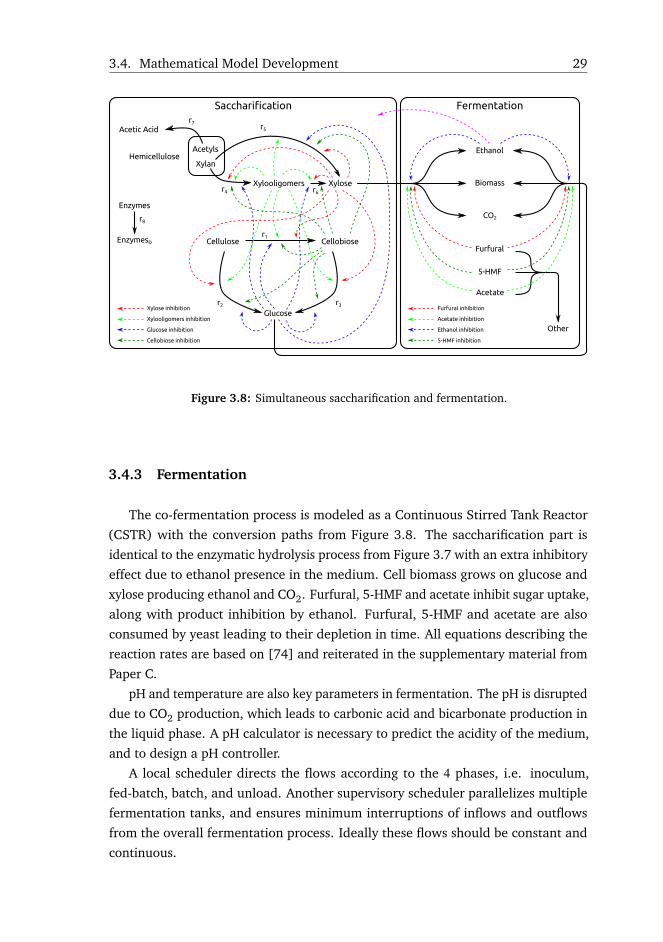
3.4. Mathematical Model Development 29
Figure 3.8: Simultaneous saccharification and fermentation.
3.4.3 Fermentation
The co-fermentation process is modeled as a Continuous Stirred Tank Reactor
(CSTR) with the conversion paths from Figure 3.8. The saccharification part is
identical to the enzymatic hydrolysis process from Figure 3.7 with an extra inhibitory
effect due to ethanol presence in the medium. Cell biomass grows on glucose and
xylose producing ethanol and CO2. Furfural, 5-HMF and acetate inhibit sugar uptake,
along with product inhibition by ethanol. Furfural, 5-HMF and acetate are also
consumed by yeast leading to their depletion in time. All equations describing the
reaction rates are based on [74] and reiterated in the supplementary material from
Paper C.
pH and temperature are also key parameters in fermentation. The pH is disrupted
due to CO2 production, which leads to carbonic acid and bicarbonate production in
the liquid phase. A pH calculator is necessary to predict the acidity of the medium,
and to design a pH controller.
A local scheduler directs the flows according to the 4 phases, i.e. inoculum,
fed-batch, batch, and unload. Another supervisory scheduler parallelizes multiple
fermentation tanks, and ensures minimum interruptions of inflows and outflows
from the overall fermentation process. Ideally these flows should be constant and
continuous.
30 Chapter 3. Dynamic Modeling and Analysis
3.4.4 Fast pH Calculations with Guaranteed Accuracy for Dynamic
Simulations
Enzymes and GMO yeast are very sensitive to pH variations following a Gaussian
bell curve that describes their efficiency with a single optimal peak. A pH calculator is
necessary for controlling and monitoring the enzymatic hydrolysis and fermentation
processes, and is embedded into the modeling library. The calculator serves as a test
bench for the pH controller designed in Chapter 5. The results from this section are
not yet published and more implementation details are offered.
There are various ways of calculating the pH of a mixture, out of which the
following three are the most used: (1) the alkalinity conservation approach, (2) the
advancement method, and the charge balance approach [75]. The methods have
several disadvantages: a numerical solver such as Newton-Raphson that often fails
to converge (1), tracking a large number of states for each ion increasing model
complexity (2), or a nonlinear equation solver that requires a long computational
time (3) [75]. Such implementations turn pH calculations into bottlenecks in
dynamic simulations.
The approach in this work is to use a reduced number of model states as in (1)
and (3), and to avoid Newton-Raphson methods (where convergence can fail) and
nonlinear equations solvers (which are slow). In contrast, the developed algorithm
utilizes a modified bisection method for finding the root of the charge balance,
which offers better convergence properties than the Newton-Raphson method and
is faster than a solver of nonlinear equations. The charge balance is processed in
order to express it as a function of only hydrogen ion concentration, which becomes
the unknown. The bisection method is modified to advance in the pH logarithmic
space while evaluating the charge balance in the state space. This method has the
advantage that it always converges to a root with a preset accuracy if the function is
monotonic and the solution can be bounded in an interval such that the function
has opposite signs at its borders. Hence it has a guaranteed accuracy property under
certain conditions. However, a higher accuracy increases the amount of convergence
steps, which slows the computational time. The solution is to exploit the dynamic
simulations and determine a tight interval around the root to be found at time
k using the previous pH solution from time k− 1. In dynamic simulations, the
integration steps are relatively close to each other and the pH is not expected to
change significantly in time, especially because it is a controlled variable kept to a
reference point. The method has been found to be fast in reality, the pH calculations
not appearing as bottlenecks in dynamic simulations anymore. Algorithm 1 illustrates
the modified bisection method while Algorithm 2 shows how to compute the bounds
around the sought solution.
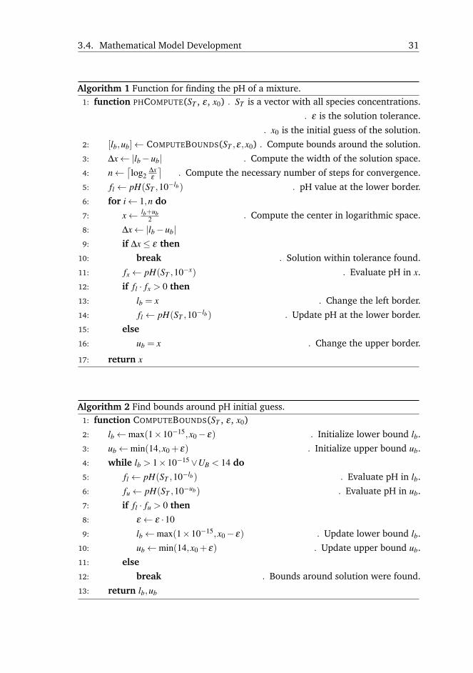
3.4. Mathematical Model Development 31
Algorithm 1 Function for finding the pH of a mixture.1: function PHCOMPUTE(ST , ε, x0) . ST is a vector with all species concentrations.
. ε is the solution tolerance.
. x0 is the initial guess of the solution.
2: [lb,ub]← COMPUTEBOUNDS(ST ,ε,x0) . Compute bounds around the solution.
3: ∆x← |lb−ub| . Compute the width of the solution space.
4: n←⌈log2
∆xε⌉
. Compute the necessary number of steps for convergence.
5: fl ← pH(ST ,10−lb) . pH value at the lower border.
6: for i← 1,n do
7: x← lb+ub2 . Compute the center in logarithmic space.
8: ∆x← |lb−ub|9: if ∆x≤ ε then
10: break . Solution within tolerance found.
11: fx← pH(ST ,10−x) . Evaluate pH in x.
12: if fl · fx > 0 then
13: lb = x . Change the left border.
14: fl ← pH(ST ,10−lb) . Update pH at the lower border.
15: else
16: ub = x . Change the upper border.
17: return x
Algorithm 2 Find bounds around pH initial guess.1: function COMPUTEBOUNDS(ST , ε, x0)
2: lb←max(1×10⁻¹⁵,x0− ε) . Initialize lower bound lb.
3: ub←min(14,x0 + ε) . Initialize upper bound ub.
4: while lb > 1×10⁻¹⁵∨UB < 14 do
5: fl ← pH(ST ,10−lb) . Evaluate pH in lb.
6: fu← pH(ST ,10−ub) . Evaluate pH in ub.
7: if fl · fu > 0 then
8: ε ← ε ·109: lb←max(1×10⁻¹⁵,x0− ε) . Update lower bound lb.
10: ub←min(14,x0 + ε) . Update upper bound ub.
11: else
12: break . Bounds around solution were found.
13: return lb,ub
32 Chapter 3. Dynamic Modeling and Analysis
The algorithm complexity is O(logn) given by the divide and conquer nature
of the bisection method, where n is the size of the solution space. The worst
case scenario corresponds to searching for the solution in the entire pH value set,
i.e. pH ∈ [0,14]. This means that ∆x = 14. If a two digits solution is sufficient
then ε = 0.01. The number of converge steps then becomes m = dlog2(1400)e= 11,
meaning that a solution with accuracy ε is found in 11 steps. Such an accuracy is
sufficient for controlling and monitoring the enzymatic hydrolysis and fermentation
processes because a deviation of 0.01 from the optimal pH value has no impact on
the process efficiency.
If the accuracy is increased, e.g. ε = 1×10⁻⁶, then the number of converge steps
in the worst case scenario becomes m =⌈log2(14×106)
⌉= 24, which is still reason-
able for nowadays computers. If the solution bounds are updated at each iteration
using the previous solution as initial guess then the number of converge steps can be
further reduced. For example, if the solution can be bounded within ∆x = 0.01 units
at each step then the solution space is significantly reduced and convergence takes
place in m =⌈log2(1×10⁴)
⌉= 14. In dynamic simulations with small integration
steps the solution can be bounded even further following the method from Algorithm
2. The higher the accuracy is demanded the more performance can be offered by
tightening the bounds around the solution.
3.4.5 Model Summary
The biorefinery model is complex and nonlinear including the most significant
phenomena reported in the literature so far. Table 3.3 lists all features of the
modeling library together with the publication that contains the full derivation
details.
When interconnecting all library modules for describing the entire refinery, the
model reaches a high complexity as in Table 3.4. The large number of states in
pretreatment and enzymatic hydrolysis is due to CFD methods, which are used for
discretizing big scale reactors. The inputs refer to feedstock mass flow, enthalpy, and
composition, while the outputs comprise the outflow, enthalpy, and composition of
the fermentation outstream. The table contains data for a single fermentation reactor
but in reality there are several tanks running in parallel, which would increase the
number of states in fermentation.
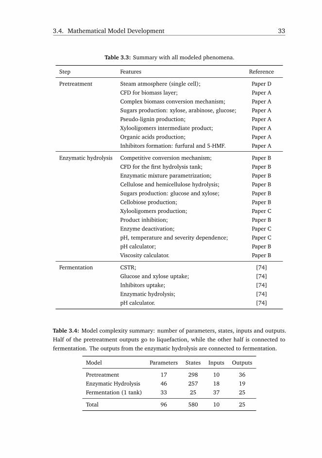
3.4. Mathematical Model Development 33
Table 3.3: Summary with all modeled phenomena.
Step Features Reference
Pretreatment Steam atmosphere (single cell); Paper D
CFD for biomass layer; Paper A
Complex biomass conversion mechanism; Paper A
Sugars production: xylose, arabinose, glucose; Paper A
Pseudo-lignin production; Paper A
Xylooligomers intermediate product; Paper A
Organic acids production; Paper A
Inhibitors formation: furfural and 5-HMF. Paper A
Enzymatic hydrolysis Competitive conversion mechanism; Paper B
CFD for the first hydrolysis tank; Paper B
Enzymatic mixture parametrization; Paper B
Cellulose and hemicellulose hydrolysis; Paper B
Sugars production: glucose and xylose; Paper B
Cellobiose production; Paper B
Xylooligomers production; Paper C
Product inhibition; Paper B
Enzyme deactivation; Paper C
pH, temperature and severity dependence; Paper C
pH calculator; Paper B
Viscosity calculator. Paper B
Fermentation CSTR; [74]
Glucose and xylose uptake; [74]
Inhibitors uptake; [74]
Enzymatic hydrolysis; [74]
pH calculator. [74]
Table 3.4: Model complexity summary: number of parameters, states, inputs and outputs.
Half of the pretreatment outputs go to liquefaction, while the other half is connected to
fermentation. The outputs from the enzymatic hydrolysis are connected to fermentation.
Model Parameters States Inputs Outputs
Pretreatment 17 298 10 36
Enzymatic Hydrolysis 46 257 18 19
Fermentation (1 tank) 33 25 37 25
Total 96 580 10 25
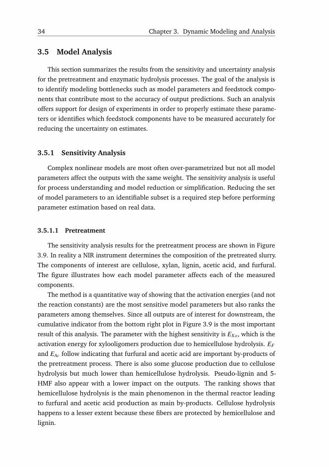
34 Chapter 3. Dynamic Modeling and Analysis
3.5 Model Analysis
This section summarizes the results from the sensitivity and uncertainty analysis
for the pretreatment and enzymatic hydrolysis processes. The goal of the analysis is
to identify modeling bottlenecks such as model parameters and feedstock compo-
nents that contribute most to the accuracy of output predictions. Such an analysis
offers support for design of experiments in order to properly estimate these parame-
ters or identifies which feedstock components have to be measured accurately for
reducing the uncertainty on estimates.
3.5.1 Sensitivity Analysis
Complex nonlinear models are most often over-parametrized but not all model
parameters affect the outputs with the same weight. The sensitivity analysis is useful
for process understanding and model reduction or simplification. Reducing the set
of model parameters to an identifiable subset is a required step before performing
parameter estimation based on real data.
3.5.1.1 Pretreatment
The sensitivity analysis results for the pretreatment process are shown in Figure
3.9. In reality a NIR instrument determines the composition of the pretreated slurry.
The components of interest are cellulose, xylan, lignin, acetic acid, and furfural.
The figure illustrates how each model parameter affects each of the measured
components.
The method is a quantitative way of showing that the activation energies (and not
the reaction constants) are the most sensitive model parameters but also ranks the
parameters among themselves. Since all outputs are of interest for downstream, the
cumulative indicator from the bottom right plot in Figure 3.9 is the most important
result of this analysis. The parameter with the highest sensitivity is EXo, which is the
activation energy for xylooligomers production due to hemicellulose hydrolysis. EF
and EAc follow indicating that furfural and acetic acid are important by-products of
the pretreatment process. There is also some glucose production due to cellulose
hydrolysis but much lower than hemicellulose hydrolysis. Pseudo-lignin and 5-
HMF also appear with a lower impact on the outputs. The ranking shows that
hemicellulose hydrolysis is the main phenomenon in the thermal reactor leading
to furfural and acetic acid production as main by-products. Cellulose hydrolysis
happens to a lesser extent because these fibers are protected by hemicellulose and
lignin.
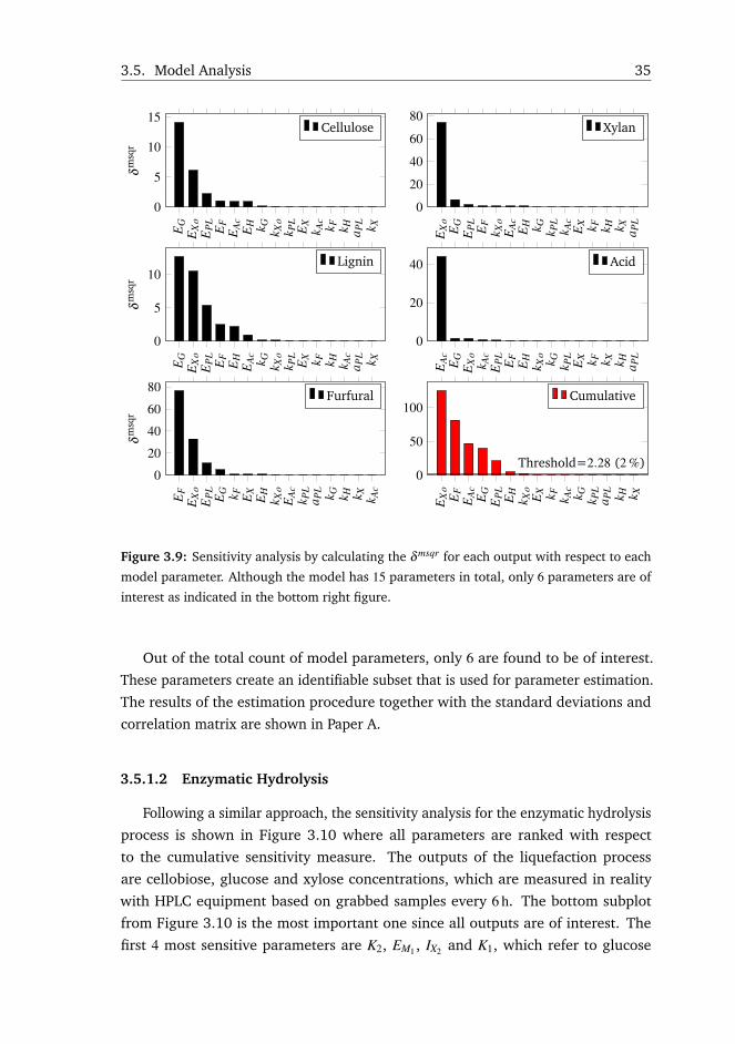
3.5. Model Analysis 35
EG
EX
oE
PL
EF
EA
cE
H k G k Xo
k PL
EX
k Ac
k F k H a PL k X
0
5
10
15δm
sqr
Cellulose
EX
oE
GE
PL
EF
k Xo
EA
cE
H k G k PL
k Ac
EX k F k H k X a PL
0
20
40
60
80Xylan
EG
EX
oE
PL
EF
EH
EA
ck G k X
ok P
LE
X k F k H k Ac
a PL k X
0
5
10
δmsq
r
Lignin
EA
cE
GE
Xo
k Ac
EP
LE
FE
Hk X
ok G k P
LE
X k F k X k H a PL
0
20
40 Acid
EF
EX
oE
PL
EG k F EX
EH
k Xo
EA
ck P
La P
L k G k H k X k Ac
0
20
40
60
80
δmsq
r
Furfural
EX
oE
FE
Ac
EG
EP
LE
Hk X
oE
X k F k Ac
k G k PL
a PL
k H k X
0
50
100
Threshold=2.28 (2 %)
Cumulative
Figure 3.9: Sensitivity analysis by calculating the δ msqr for each output with respect to each
model parameter. Although the model has 15 parameters in total, only 6 parameters are of
interest as indicated in the bottom right figure.
Out of the total count of model parameters, only 6 are found to be of interest.
These parameters create an identifiable subset that is used for parameter estimation.
The results of the estimation procedure together with the standard deviations and
correlation matrix are shown in Paper A.
3.5.1.2 Enzymatic Hydrolysis
Following a similar approach, the sensitivity analysis for the enzymatic hydrolysis
process is shown in Figure 3.10 where all parameters are ranked with respect
to the cumulative sensitivity measure. The outputs of the liquefaction process
are cellobiose, glucose and xylose concentrations, which are measured in reality
with HPLC equipment based on grabbed samples every 6 h. The bottom subplot
from Figure 3.10 is the most important one since all outputs are of interest. The
first 4 most sensitive parameters are K2, EM1 , IX2 and K1, which refer to glucose
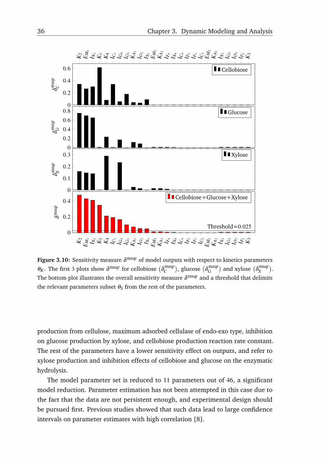
36 Chapter 3. Dynamic Modeling and Analysis
K2
EM
1
I X2
K1
K4
I C1
I G4
I G1
KA
1
I G2
I X1
EM
3
KA
3
I F4
I X4
I C4
I F3
I F1
I C2
EM
2
KA
2
I X3
I G3
I O3
I F2
K3
0
0.2
0.4
0.6
δmsq
rC
Cellobiose
0
0.2
0.4
0.6
0.8
δmsq
rG
Glucose
0
0.1
0.2
0.3
δmsq
rX
Xylose
K2
EM
1
I X2
K1
K4
I C1
I G4
I G1
KA
1
I G2
I X1
EM
3
KA
3
I F4
I X4
I C4
I F3
I F1
I C2
EM
2
KA
2
I X3
I G3
I O3
I F2
K3
0
0.2
0.4
Threshold=0.025
δmsq
r
Cellobiose+Glucose+Xylose
Figure 3.10: Sensitivity measure δ msqr of model outputs with respect to kinetics parameters
θK . The first 3 plots show δ msqr for cellobiose(δ msqr
C), glucose
(δ msqr
G)
and xylose(δ msqr
X).
The bottom plot illustrates the overall sensitivity measure δ msqr and a threshold that delimits
the relevant parameters subset θS from the rest of the parameters.
production from cellulose, maximum adsorbed cellulase of endo-exo type, inhibition
on glucose production by xylose, and cellobiose production reaction rate constant.
The rest of the parameters have a lower sensitivity effect on outputs, and refer to
xylose production and inhibition effects of cellobiose and glucose on the enzymatic
hydrolysis.
The model parameter set is reduced to 11 parameters out of 46, a significant
model reduction. Parameter estimation has not been attempted in this case due to
the fact that the data are not persistent enough, and experimental design should
be pursued first. Previous studies showed that such data lead to large confidence
intervals on parameter estimates with high correlation [8].
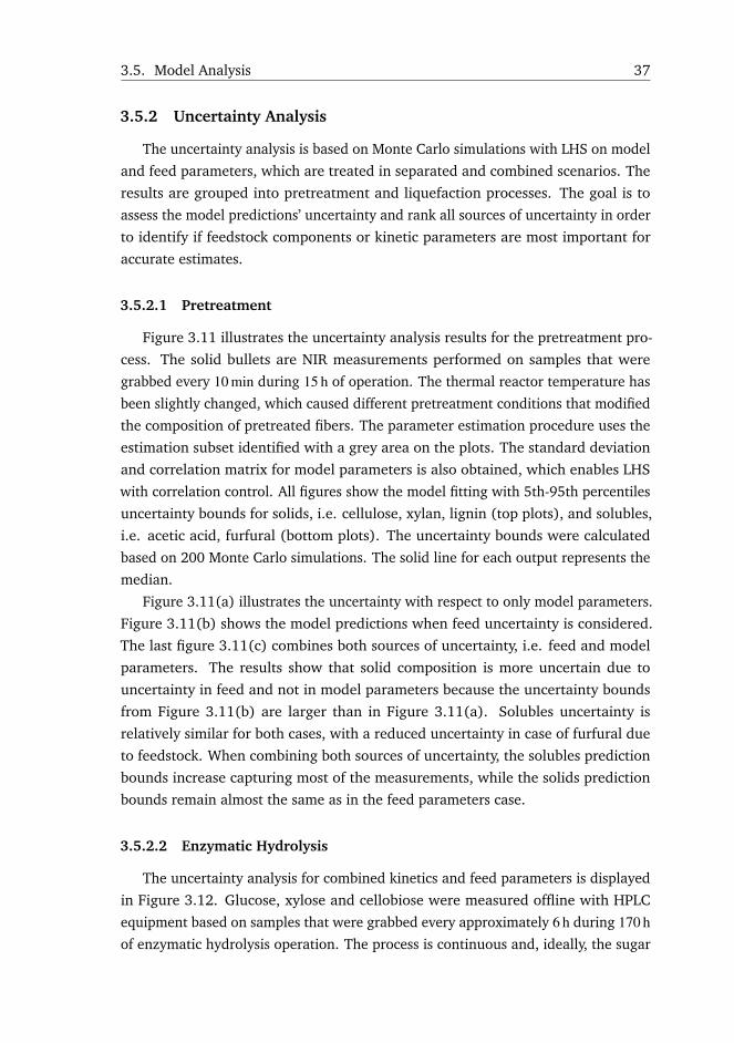
3.5. Model Analysis 37
3.5.2 Uncertainty Analysis
The uncertainty analysis is based on Monte Carlo simulations with LHS on model
and feed parameters, which are treated in separated and combined scenarios. The
results are grouped into pretreatment and liquefaction processes. The goal is to
assess the model predictions’ uncertainty and rank all sources of uncertainty in order
to identify if feedstock components or kinetic parameters are most important for
accurate estimates.
3.5.2.1 Pretreatment
Figure 3.11 illustrates the uncertainty analysis results for the pretreatment pro-
cess. The solid bullets are NIR measurements performed on samples that were
grabbed every 10 min during 15 h of operation. The thermal reactor temperature has
been slightly changed, which caused different pretreatment conditions that modified
the composition of pretreated fibers. The parameter estimation procedure uses the
estimation subset identified with a grey area on the plots. The standard deviation
and correlation matrix for model parameters is also obtained, which enables LHS
with correlation control. All figures show the model fitting with 5th-95th percentiles
uncertainty bounds for solids, i.e. cellulose, xylan, lignin (top plots), and solubles,
i.e. acetic acid, furfural (bottom plots). The uncertainty bounds were calculated
based on 200 Monte Carlo simulations. The solid line for each output represents the
median.
Figure 3.11(a) illustrates the uncertainty with respect to only model parameters.
Figure 3.11(b) shows the model predictions when feed uncertainty is considered.
The last figure 3.11(c) combines both sources of uncertainty, i.e. feed and model
parameters. The results show that solid composition is more uncertain due to
uncertainty in feed and not in model parameters because the uncertainty bounds
from Figure 3.11(b) are larger than in Figure 3.11(a). Solubles uncertainty is
relatively similar for both cases, with a reduced uncertainty in case of furfural due
to feedstock. When combining both sources of uncertainty, the solubles prediction
bounds increase capturing most of the measurements, while the solids prediction
bounds remain almost the same as in the feed parameters case.
3.5.2.2 Enzymatic Hydrolysis
The uncertainty analysis for combined kinetics and feed parameters is displayed
in Figure 3.12. Glucose, xylose and cellobiose were measured offline with HPLC
equipment based on samples that were grabbed every approximately 6 h during 170 hof enzymatic hydrolysis operation. The process is continuous and, ideally, the sugar
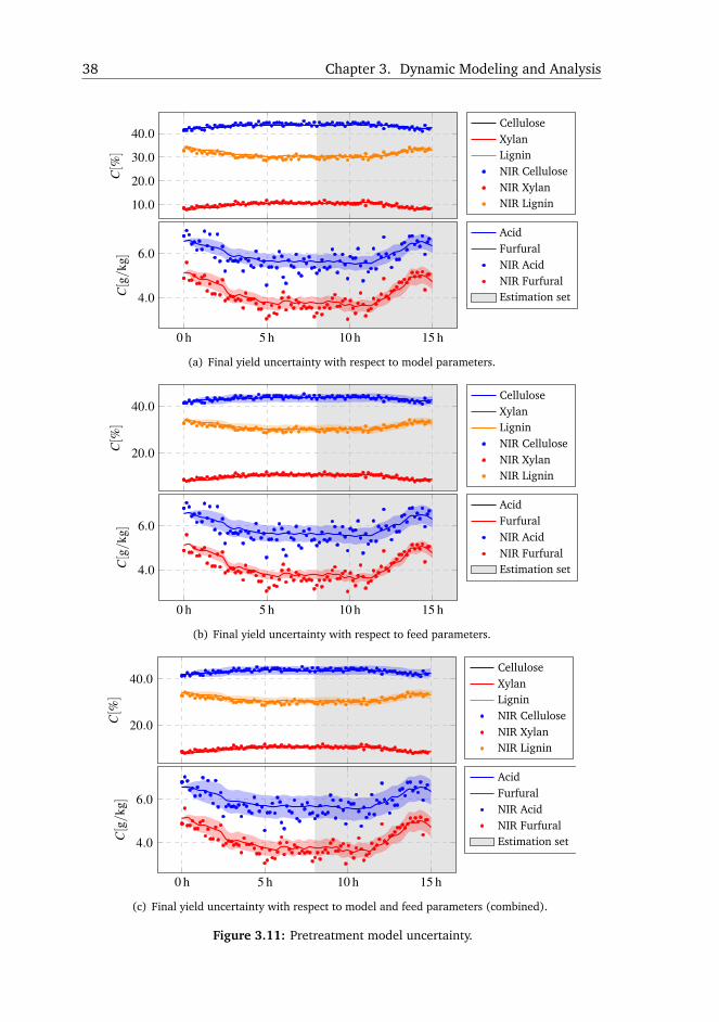
38 Chapter 3. Dynamic Modeling and Analysis
10.0
20.0
30.0
40.0
C[%
]CelluloseXylanLigninNIR CelluloseNIR XylanNIR Lignin
0 h 5 h 10 h 15 h
4.0
6.0
C[g/k
g]
AcidFurfuralNIR AcidNIR FurfuralEstimation set
(a) Final yield uncertainty with respect to model parameters.
20.0
40.0
C[%
]
CelluloseXylanLigninNIR CelluloseNIR XylanNIR Lignin
0 h 5 h 10 h 15 h
4.0
6.0
C[g/k
g]
AcidFurfuralNIR AcidNIR FurfuralEstimation set
(b) Final yield uncertainty with respect to feed parameters.
20.0
40.0
C[%
]
CelluloseXylanLigninNIR CelluloseNIR XylanNIR Lignin
0 h 5 h 10 h 15 h
4.0
6.0
C[g/k
g]
AcidFurfuralNIR AcidNIR FurfuralEstimation set
(c) Final yield uncertainty with respect to model and feed parameters (combined).
Figure 3.11: Pretreatment model uncertainty.
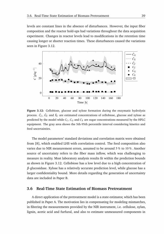
3.6. Real-Time State Estimation of Biomass Pretreatment 39
levels are constant lines in the absence of disturbances. However, the input fiber
composition and the reactor hold-ups had variations throughout the data acquisition
experiment. Changes in reactor levels lead to modifications in the retention time
causing longer or shorter reaction times. These disturbances caused the variations
seen in Figure 3.12.
0 20 40 60 80 100 120 140 160 180
0
20
40
Time [h]
C[g
kg−
1 ]
CG
CX
CCCCCGCXCI
Figure 3.12: Cellobiose, glucose and xylose formation during the enzymatic hydrolysis
process. CC, GC and XC are estimated concentrations of cellobiose, glucose and xylose as
predicted by the model while CC, CG and CX are sugar concentrations measured by the HPLC
equipment. The gray area shows the 5th-95th percentile interval considering kinetics and
feed uncertainties.
The model parameters’ standard deviations and correlation matrix were obtained
from [8], which enabled LHS with correlation control. The feed composition also
varies due to NIR measurement errors, assumed to be around 5 % to 10 %. Another
source of uncertainty refers to the fiber mass inflow, which was challenging to
measure in reality. Most laboratory analysis results fit within the prediction bounds
as shown in Figure 3.12. Cellobiose has a low level due to a high concentration of
β -glucosidase. Xylose has a relatively accurate prediction level, while glucose has a
larger confidentiality bound. More details regarding the generation of uncertainty
data are included in Paper B.
3.6 Real-Time State Estimation of Biomass Pretreatment
A direct application of the pretreatment model is a state estimator, which has been
published in Paper A. The motivation lies in compensating for modeling mismatches,
in filtering the measurements provided by the NIR instrument, i.e. cellulose, xylan,
lignin, acetic acid and furfural, and also to estimate unmeasured components in
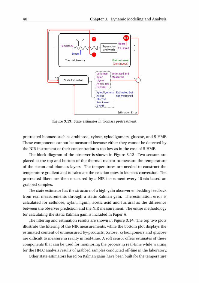
40 Chapter 3. Dynamic Modeling and Analysis
Figure 3.13: State estimator in biomass pretreatment.
pretreated biomass such as arabinose, xylose, xylooligomers, glucose, and 5-HMF.
These components cannot be measured because either they cannot be detected by
the NIR instrument or their concentration is too low as in the case of 5-HMF.
The block diagram of the observer is shown in Figure 3.13. Two sensors are
placed at the top and bottom of the thermal reactor to measure the temperature
of the steam and biomass layers. The temperatures are needed to construct the
temperature gradient and to calculate the reaction rates in biomass conversion. The
pretreated fibers are then measured by a NIR instrument every 10 min based on
grabbed samples.
The state estimator has the structure of a high-gain observer embedding feedback
from real measurements through a static Kalman gain. The estimation error is
calculated for cellulose, xylan, lignin, acetic acid and furfural as the difference
between the observer prediction and the NIR measurement. The entire methodology
for calculating the static Kalman gain is included in Paper A.
The filtering and estimation results are shown in Figure 3.14. The top two plots
illustrate the filtering of the NIR measurements, while the bottom plot displays the
estimated content of unmeasured by-products. Xylose, xylooligomers and glucose
are difficult to measure in reality in real-time. A soft sensor offers estimates of these
components that can be used for monitoring the process in real-time while waiting
for the HPLC analysis results of grabbed samples conducted off-line in the laboratory.
Other state estimators based on Kalman gains have been built for the temperature
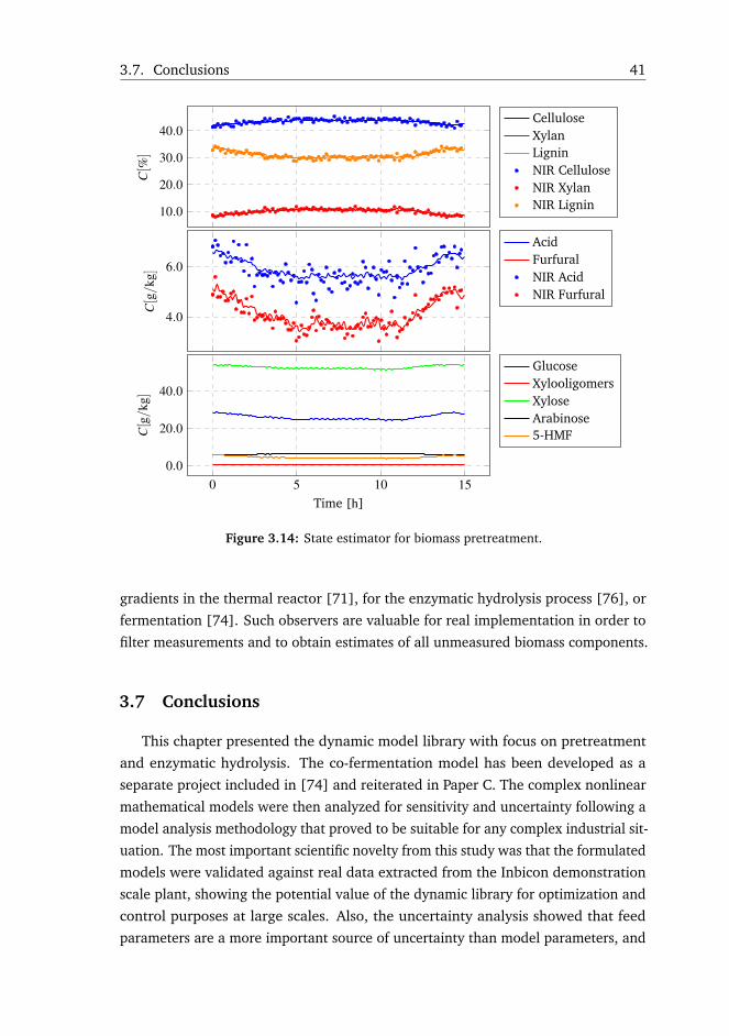
3.7. Conclusions 41
10.0
20.0
30.0
40.0C[%
]
CelluloseXylanLigninNIR CelluloseNIR XylanNIR Lignin
4.0
6.0
C[g/k
g]
AcidFurfuralNIR AcidNIR Furfural
0 5 10 150.0
20.0
40.0
Time [h]
C[g/
kg]
GlucoseXylooligomersXyloseArabinose5-HMF
Figure 3.14: State estimator for biomass pretreatment.
gradients in the thermal reactor [71], for the enzymatic hydrolysis process [76], or
fermentation [74]. Such observers are valuable for real implementation in order to
filter measurements and to obtain estimates of all unmeasured biomass components.
3.7 Conclusions
This chapter presented the dynamic model library with focus on pretreatment
and enzymatic hydrolysis. The co-fermentation model has been developed as a
separate project included in [74] and reiterated in Paper C. The complex nonlinear
mathematical models were then analyzed for sensitivity and uncertainty following a
model analysis methodology that proved to be suitable for any complex industrial sit-
uation. The most important scientific novelty from this study was that the formulated
models were validated against real data extracted from the Inbicon demonstration
scale plant, showing the potential value of the dynamic library for optimization and
control purposes at large scales. Also, the uncertainty analysis showed that feed
parameters are a more important source of uncertainty than model parameters, and
42 Chapter 3. Dynamic Modeling and Analysis
focus should be placed on measuring feed composition more accurately.
The mathematical models need maintenance and should be extended as new
phenomena appear in the scientific literature. A list with possible extensions include:
• Phenolics production in pretreatment and inhibition on the enzymatic activity
[77];
• The irreversible deactivation of enzymes in time should be a function of
temperature level and ethanol content [78], and not a constant;
• The fermentation temperature should actually follow a profile reflecting the
best compromise between enzymatic activity and GMO yeast [79]. The cal-
culation of the optimal temperature setpoint profile requires temperature
dependent model parameters for fermentation [80], which are missing in this
study.
Chapter 4
Process Optimization
4.1 Introduction
This chapter deals with designing a steady-state optimization layer for a large
scale biorefinery. The objective is to maximize the operational profit by finding
optimal key process parameters such as pretreatment temperature, enzyme dosage
in liquefaction and yeast seed in fermentation. The refinery is treated in an integrated
manner taking into account the trade-offs between the conversion steps. The detailed
methodology and results are included in Paper C.
The method is compared against a traditional refinery operation, i.e. a fixed
recipe with constant enzyme dosage and yeast seed that were determined based on
a long time experience. Sensitivity and uncertainty analysis with respect to model
and feed parameters increase the trust in the optimization layer. The chapter ends
with conclusions and suggestions for future improvements.
4.2 Plantwide Optimization Methodology
Figure 4.1 illustrates the workflow interactions between the real plant and the
layers for control, optimization and system identification. Each conversion stage
from the real plant is equipped with specific sensors and actuators that enable fast
feedback control for tracking the pretreatment temperature, enzyme dosage and
yeast seed. An advanced reference tracking controller for biomass pretreatment
temperature has been developed in [6]. An enzyme dosage regulator can be easily
constructed with a flow meter and a variable valve mounted on the enzyme supply
pipe. The enzymatic hydrolysis process is continuous and the enzyme dosage
stabilizes to a non-zero value. The yeast seed controller requires a mass estimator
and a control valve on the supply pipe. The fermentation process runs in batches,
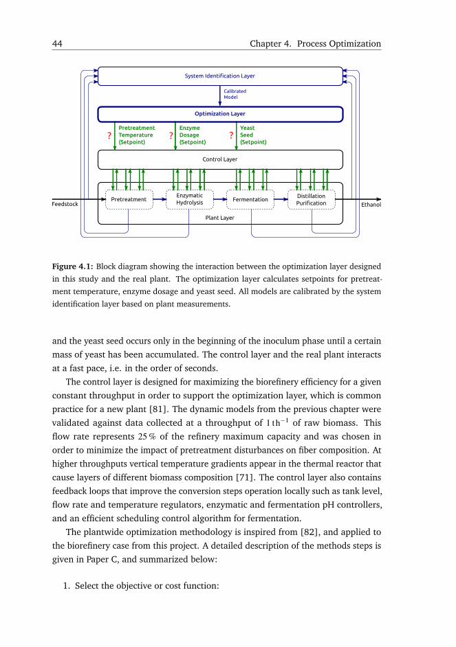
44 Chapter 4. Process Optimization
Figure 4.1: Block diagram showing the interaction between the optimization layer designed
in this study and the real plant. The optimization layer calculates setpoints for pretreat-
ment temperature, enzyme dosage and yeast seed. All models are calibrated by the system
identification layer based on plant measurements.
and the yeast seed occurs only in the beginning of the inoculum phase until a certain
mass of yeast has been accumulated. The control layer and the real plant interacts
at a fast pace, i.e. in the order of seconds.
The control layer is designed for maximizing the biorefinery efficiency for a given
constant throughput in order to support the optimization layer, which is common
practice for a new plant [81]. The dynamic models from the previous chapter were
validated against data collected at a throughput of 1 th−1 of raw biomass. This
flow rate represents 25 % of the refinery maximum capacity and was chosen in
order to minimize the impact of pretreatment disturbances on fiber composition. At
higher throughputs vertical temperature gradients appear in the thermal reactor that
cause layers of different biomass composition [71]. The control layer also contains
feedback loops that improve the conversion steps operation locally such as tank level,
flow rate and temperature regulators, enzymatic and fermentation pH controllers,
and an efficient scheduling control algorithm for fermentation.
The plantwide optimization methodology is inspired from [82], and applied to
the biorefinery case from this project. A detailed description of the methods steps is
given in Paper C, and summarized below:
1. Select the objective or cost function:
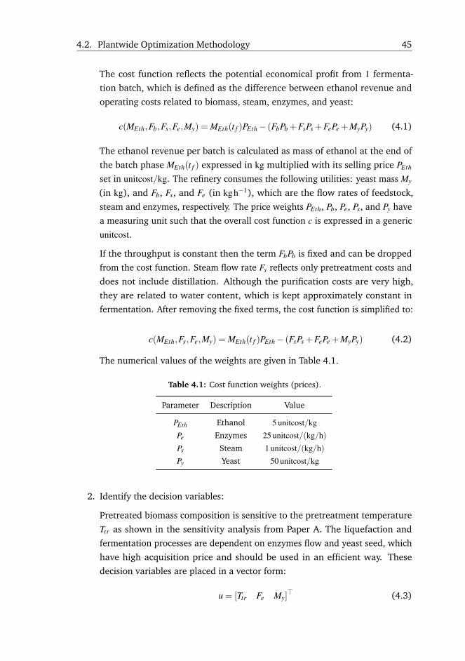
4.2. Plantwide Optimization Methodology 45
The cost function reflects the potential economical profit from 1 fermenta-
tion batch, which is defined as the difference between ethanol revenue and
operating costs related to biomass, steam, enzymes, and yeast:
c(MEth,Fb,Fs,Fe,My) = MEth(t f )PEth− (FbPb +FsPs +FePe +MyPy) (4.1)
The ethanol revenue per batch is calculated as mass of ethanol at the end of
the batch phase MEth(t f ) expressed in kg multiplied with its selling price PEth
set in unitcost/kg. The refinery consumes the following utilities: yeast mass My
(in kg), and Fb, Fs, and Fe (in kgh−1), which are the flow rates of feedstock,
steam and enzymes, respectively. The price weights PEth, Pb, Pe, Ps, and Py have
a measuring unit such that the overall cost function c is expressed in a generic
unitcost.
If the throughput is constant then the term FbPb is fixed and can be dropped
from the cost function. Steam flow rate Fs reflects only pretreatment costs and
does not include distillation. Although the purification costs are very high,
they are related to water content, which is kept approximately constant in
fermentation. After removing the fixed terms, the cost function is simplified to:
c(MEth,Fs,Fe,My) = MEth(t f )PEth− (FsPs +FePe +MyPy) (4.2)
The numerical values of the weights are given in Table 4.1.
Table 4.1: Cost function weights (prices).
Parameter Description Value
PEth Ethanol 5 unitcost/kg
Pe Enzymes 25 unitcost/(kg/h)
Ps Steam 1 unitcost/(kg/h)
Py Yeast 50 unitcost/kg
2. Identify the decision variables:
Pretreated biomass composition is sensitive to the pretreatment temperature
Ttr as shown in the sensitivity analysis from Paper A. The liquefaction and
fermentation processes are dependent on enzymes flow and yeast seed, which
have high acquisition price and should be used in an efficient way. These
decision variables are placed in a vector form:
u = [Ttr Fe My]> (4.3)
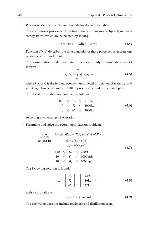
46 Chapter 4. Process Optimization
3. Process model constraints, and bounds for decision variables:
The continuous processes of pretreatment and enzymatic hydrolysis reach
steady states, which are calculated by solving:
x = f (x,u) when x = 0 (4.4)
Function f (x,u) describes the time dynamics of these processes as expressions
of state vector x and input u.
The fermentation model is a batch process and only the final states are of
interest:
x f (t f ) =
t f∫0
h(x f ,u f )dt (4.5)
where h(x f ,u f ) is the fermentation dynamic model as function of states x f , and
inputs u f . Time constant t f = 190h represents the end of the batch phase.
The decision variables are bounded as follows:
150 ≤ Ttr ≤ 210 ◦C10 ≤ Fe ≤ 1000kgh−1
10 ≤ My ≤ 1000kg
(4.6)
reflecting a wide range of operation.
4. Formulate and solve the overall optimization problem:
maxTtr ,Fe,My
MEth(t f )PEth− (FsPs +FePe +MyPy)
subject to 0 = f (x(t),u(t))
x f = h(x f ,u f )
150 ≤ Ttr ≤ 210 ◦C10 ≤ Fe ≤ 1000kgh−1
10 ≤ My ≤ 1000kg
(4.7)
The following solution is found:
zo =
Ttr
Fe
My
=
172 ◦C110kgh−1
142kg
(4.8)
with a cost value of:
co = 76714unitprofit (4.9)
The cost value does not include feedstock and distillation costs.
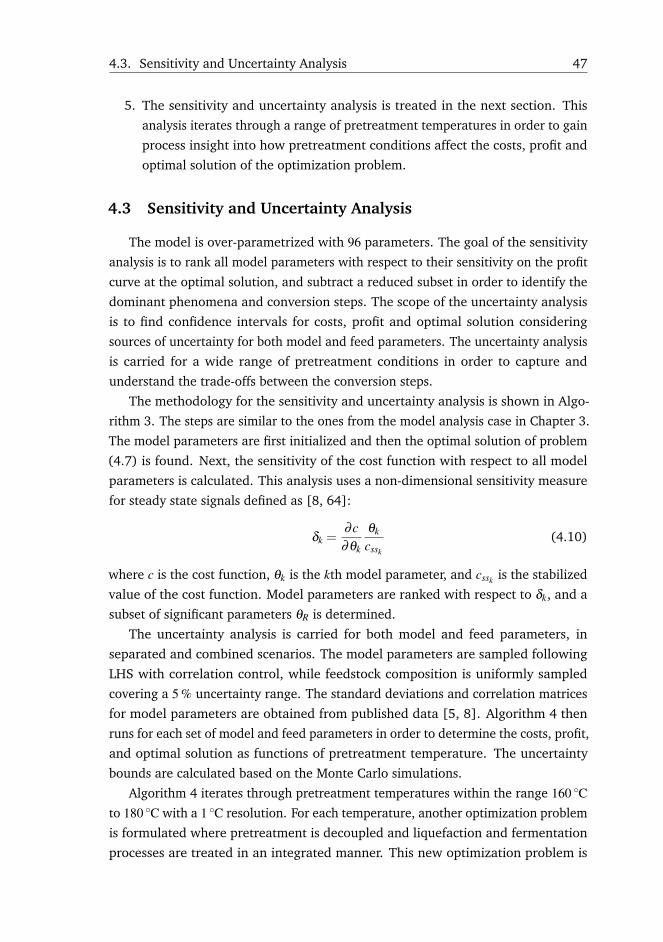
4.3. Sensitivity and Uncertainty Analysis 47
5. The sensitivity and uncertainty analysis is treated in the next section. This
analysis iterates through a range of pretreatment temperatures in order to gain
process insight into how pretreatment conditions affect the costs, profit and
optimal solution of the optimization problem.
4.3 Sensitivity and Uncertainty Analysis
The model is over-parametrized with 96 parameters. The goal of the sensitivity
analysis is to rank all model parameters with respect to their sensitivity on the profit
curve at the optimal solution, and subtract a reduced subset in order to identify the
dominant phenomena and conversion steps. The scope of the uncertainty analysis
is to find confidence intervals for costs, profit and optimal solution considering
sources of uncertainty for both model and feed parameters. The uncertainty analysis
is carried for a wide range of pretreatment conditions in order to capture and
understand the trade-offs between the conversion steps.
The methodology for the sensitivity and uncertainty analysis is shown in Algo-
rithm 3. The steps are similar to the ones from the model analysis case in Chapter 3.
The model parameters are first initialized and then the optimal solution of problem
(4.7) is found. Next, the sensitivity of the cost function with respect to all model
parameters is calculated. This analysis uses a non-dimensional sensitivity measure
for steady state signals defined as [8, 64]:
δk =∂c∂θk
θk
cssk
(4.10)
where c is the cost function, θk is the kth model parameter, and cssk is the stabilized
value of the cost function. Model parameters are ranked with respect to δk, and a
subset of significant parameters θR is determined.
The uncertainty analysis is carried for both model and feed parameters, in
separated and combined scenarios. The model parameters are sampled following
LHS with correlation control, while feedstock composition is uniformly sampled
covering a 5 % uncertainty range. The standard deviations and correlation matrices
for model parameters are obtained from published data [5, 8]. Algorithm 4 then
runs for each set of model and feed parameters in order to determine the costs, profit,
and optimal solution as functions of pretreatment temperature. The uncertainty
bounds are calculated based on the Monte Carlo simulations.
Algorithm 4 iterates through pretreatment temperatures within the range 160 ◦Cto 180 ◦C with a 1 ◦C resolution. For each temperature, another optimization problem
is formulated where pretreatment is decoupled and liquefaction and fermentation
processes are treated in an integrated manner. This new optimization problem is
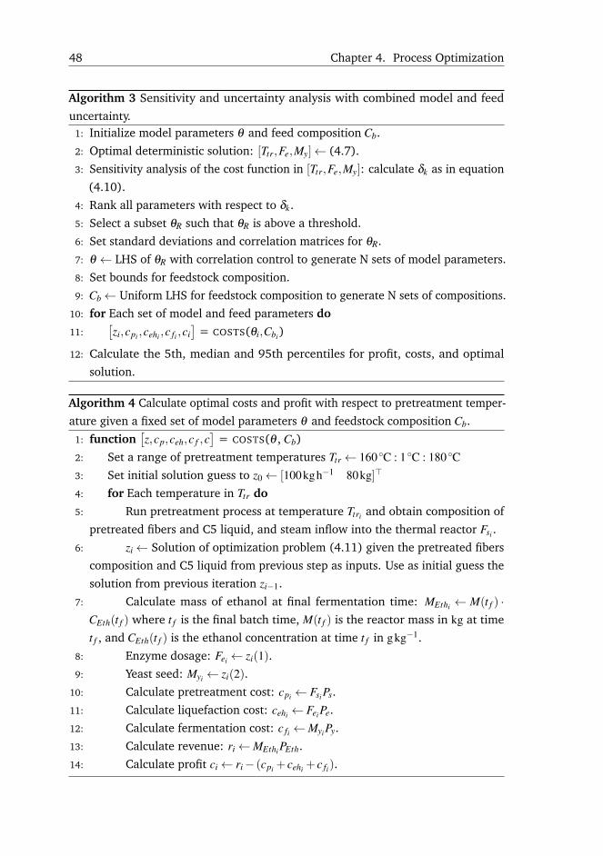
48 Chapter 4. Process Optimization
Algorithm 3 Sensitivity and uncertainty analysis with combined model and feed
uncertainty.1: Initialize model parameters θ and feed composition Cb.
2: Optimal deterministic solution: [Ttr,Fe,My]← (4.7).
3: Sensitivity analysis of the cost function in [Ttr,Fe,My]: calculate δk as in equation
(4.10).
4: Rank all parameters with respect to δk.
5: Select a subset θR such that θR is above a threshold.
6: Set standard deviations and correlation matrices for θR.
7: θ ← LHS of θR with correlation control to generate N sets of model parameters.
8: Set bounds for feedstock composition.
9: Cb← Uniform LHS for feedstock composition to generate N sets of compositions.
10: for Each set of model and feed parameters do
11:[zi,cpi ,cehi ,c fi ,ci
]= COSTS(θi,Cbi)
12: Calculate the 5th, median and 95th percentiles for profit, costs, and optimal
solution.
Algorithm 4 Calculate optimal costs and profit with respect to pretreatment temper-
ature given a fixed set of model parameters θ and feedstock composition Cb.
1: function[z,cp,ceh,c f ,c
]= COSTS(θ , Cb)
2: Set a range of pretreatment temperatures Ttr← 160 ◦C : 1 ◦C : 180 ◦C3: Set initial solution guess to z0← [100kgh−1 80kg]>
4: for Each temperature in Ttr do
5: Run pretreatment process at temperature Ttri and obtain composition of
pretreated fibers and C5 liquid, and steam inflow into the thermal reactor Fsi .
6: zi← Solution of optimization problem (4.11) given the pretreated fibers
composition and C5 liquid from previous step as inputs. Use as initial guess the
solution from previous iteration zi−1.
7: Calculate mass of ethanol at final fermentation time: MEthi ← M(t f ) ·CEth(t f ) where t f is the final batch time, M(t f ) is the reactor mass in kg at time
t f , and CEth(t f ) is the ethanol concentration at time t f in gkg−1.
8: Enzyme dosage: Fei ← zi(1).9: Yeast seed: Myi ← zi(2).
10: Calculate pretreatment cost: cpi ← FsiPs.
11: Calculate liquefaction cost: cehi ← FeiPe.
12: Calculate fermentation cost: c fi ←MyiPy.
13: Calculate revenue: ri←MEthiPEth.
14: Calculate profit ci← ri− (cpi + cehi + c fi).
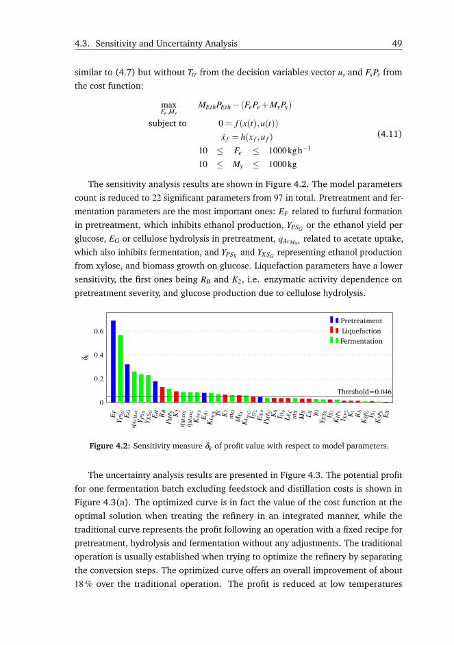
4.3. Sensitivity and Uncertainty Analysis 49
similar to (4.7) but without Ttr from the decision variables vector u, and FsPs from
the cost function:
maxFe,My
MEthPEth− (FePe +MyPy)
subject to 0 = f (x(t),u(t))
x f = h(x f ,u f )
10 ≤ Fe ≤ 1000kgh−1
10 ≤ My ≤ 1000kg
(4.11)
The sensitivity analysis results are shown in Figure 4.2. The model parameters
count is reduced to 22 significant parameters from 97 in total. Pretreatment and fer-
mentation parameters are the most important ones: EF related to furfural formation
in pretreatment, which inhibits ethanol production, YPSG or the ethanol yield per
glucose, EG or cellulose hydrolysis in pretreatment, qAcMax related to acetate uptake,
which also inhibits fermentation, and YPSX and YXSG representing ethanol production
from xylose, and biomass growth on glucose. Liquefaction parameters have a lower
sensitivity, the first ones being RB and K2, i.e. enzymatic activity dependence on
pretreatment severity, and glucose production due to cellulose hydrolysis.
EF
Y PS G EG
q Ac M
axY P
S XY X
S G EH RB
P MP X K
2q M
axX
q Max
GK
Ac S
EA
cK
I Ac X γ X K
7m
GM
E CK
I Ac G I G
2E
Xo
P MP G K
6I O
6L E
Cm
XM
X L X γ GY X
S X I X2
KIP
XI X
o 2 K1
RA
KSP
GI X
1K
SPX
EX
0
0.2
0.4
0.6
Threshold=0.046
δ k
PretreatmentLiquefactionFermentation
Figure 4.2: Sensitivity measure δk of profit value with respect to model parameters.
The uncertainty analysis results are presented in Figure 4.3. The potential profit
for one fermentation batch excluding feedstock and distillation costs is shown in
Figure 4.3(a). The optimized curve is in fact the value of the cost function at the
optimal solution when treating the refinery in an integrated manner, while the
traditional curve represents the profit following an operation with a fixed recipe for
pretreatment, hydrolysis and fermentation without any adjustments. The traditional
operation is usually established when trying to optimize the refinery by separating
the conversion steps. The optimized curve offers an overall improvement of about
18 % over the traditional operation. The profit is reduced at low temperatures
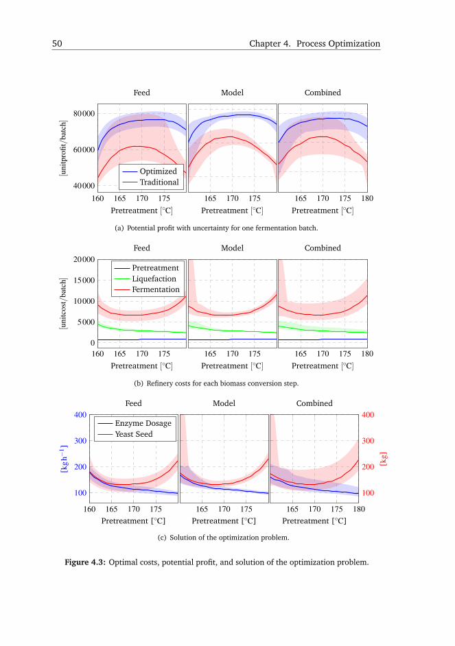
50 Chapter 4. Process Optimization
160 165 170 175
40000
60000
80000
Pretreatment [◦C]
[uni
tpro
fit/b
atch]
Feed
OptimizedTraditional
165 170 175Pretreatment [◦C]
Model
165 170 175 180Pretreatment [◦C]
Combined
(a) Potential profit with uncertainty for one fermentation batch.
160 165 170 1750
5000
10000
15000
20000
Pretreatment [◦C]
[uni
tcos
t/ba
tch]
Feed
PretreatmentLiquefactionFermentation
165 170 175Pretreatment [◦C]
Model
165 170 175 180Pretreatment [◦C]
Combined
(b) Refinery costs for each biomass conversion step.
160 165 170 175
100
200
300
400
Pretreatment [◦C]
[kg
h−1 ]
Feed
Enzyme DosageYeast Seed
165 170 175Pretreatment [◦C]
Model
165 170 175 180
100
200
300
400
Pretreatment [◦C]
[kg]
Combined
(c) Solution of the optimization problem.
Figure 4.3: Optimal costs, potential profit, and solution of the optimization problem.
4.4. Conclusions 51
because the biomatrix is not sufficiently open, and hemicellulose is not hydrolyzed
enough. A low pretreatment temperature requires more enzymes and yeast to
compensate for hardly accessible cellulose, also indicated in the solution plots from
Figure 4.3(c). At higher pretreatment temperatures inhibitors become significant and
decrease ethanol yield causing a lower profit. The optimal pretreatment temperature
is found to be around 172 ◦C. Another important aspect is that feed dominates
model parameters uncertainty. Accurate measurements on feedstock are required
to decrease the uncertainty on the potential profit of the refinery process. Model
uncertainty also decreases as temperature increases due to the fact that biomatrix
opening reduces its significance on model predictions. Overall the optimized profit
curve has a lower uncertainty than the traditional operation because the enzyme
dosage and yeast seed are adjusted with respect to pretreatment conditions.
Figure 4.3(c) shows the solution of the optimization problem as a function
of pretreatment temperature. The amount of enzymes decrease as pretreatment
temperature increases showing that a high pretreatment is beneficial for enzymatic
hydrolysis, while negative for fermentation due to inhibitors creation. The yeast
curve has a U shape. At low temperatures, a higher amount of yeast accelerates the
simultaneous saccharification and fermentation process while at higher temperature
more yeast compensates for the inhibitors. The refinery costs are proportional to the
solution of the optimization problem, and detailed in Figure 4.3(b).
4.4 Conclusions
This chapter presented the results from Paper C, i.e. a study on economical opti-
mization of a large scale second generation biorefinery in a simulated environment.
The optimization procedure makes use of steady-state models for pretreatment and
enzymatic hydrolysis, and a dynamic fermentation model. The process key parame-
ters are the pretreatment temperature, enzyme dosage in liquefaction, and yeast seed
in fermentation. A high pretreatment temperature was found to be positive for the
performance of enzymatic hydrolysis but negative for ethanol yield due to creation of
inhibitors. Uncertainties in kinetics of pretreatment, liquefaction and fermentation
were quantified as negligible on the economic objective function around the optimal
operational point. The main source of uncertainty was found to be in the inflow feed
composition.
The enzymatic hydrolysis and fermentation are connected in series in this study
as in the second version of Inbicon. However, the same methodology can be applied
in the case of a fermentation broth recycle that would enable enzymes reuse [83].
The optimization was carried at constant given throughput. As a future improve-
52 Chapter 4. Process Optimization
ment, the biorefinery throughput can be added as a degree of freedom that would
allow searching for a higher throughput such that profit is maximized [84]. In
reality, the optimal profit value is slightly degraded due to the compromise between
hydrolysis and optimal fermentation temperature [85], which decreases ethanol
yield or would require a higher amount of enzymes and yeast to compensate. An
optimal temperature profile can be calculated for maximizing the ethanol yield [79].
In fermentation, feed rate control boosts the performance by maximizing the specific
growth rate while avoiding accumulation of inhibitors [86]. Also, in the case of
glucose fermentation, the amount of necessary yeast can be significantly reduced by
calculating an optimal feed rate profile during the fed-batch phase while avoiding
accumulation of inhibitors as in Section 5.4.
For ensuring the successfulness of the optimization method, the control layer
and the process architectural setup should be solved in an integrated manner and
not sequentially as is common practice in the industry [87]. The contribution of this
study is to offer support for additional changes that are necessary to improve the
biorefinery design. The results from this chapter were based on several assumptions
regarding available measurements and control strategies, which should be included
in future plant versions: feedstock NIR measurements, and control on enzymes flow
rate and yeast dosage.
Chapter 5
Advanced Process Control
5.1 Introduction
This chapter presents the main results from two IEEE peer-reviewed conference
publications included in the appendix as Papers E and D, as well as unpublished
results regarding an optimal feed rate profile of liquefied fibers in glucose fermen-
tation that minimizes the yeast seed and avoids accumulation of inhibitors. The
IEEE conference contributions deal with two applications of the L1 adaptive output
feedback controller: one for regulating the temperature in the pretreatment ther-
mal reactor, and another one for keeping the pH level close to its optimum in the
enzymatic hydrolysis process.
5.2 Pretreatment Temperature Control
The sensitivity analysis for the hydrothermal biomass pretreatment model from
Section 3.5.1.1 showed that the activation energies of conversion reactions in the
thermal reactor are sensitive for pretreated biomass composition. That is also the
reason why the pretreatment temperature is one of the decision variables in the
optimization layer. These facts show that a temperature controller is necessary
to ensure little variations from the desired reaction temperature, and to transit
smoothly to the setpoint given by the optimization layer.
The particle pump pressurizes biomass till the thermal reactor pressure based
on the following cycle: an amount of soaked fibers is first trapped in the particle
pump chamber with the help of a pushing snail; the thermal reactor pressure is then
reached by opening a steam valve from a pipe that interconnects the reactor and the
particle pump; once the same pressure level is reached, the steam valve is closed,
and the biomass is released inside the thermal reactor. The total duration of the
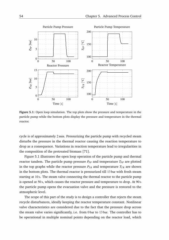
54 Chapter 5. Advanced Process Control
0 50 1000
5
10
P PP[b
ar]
Particle Pump Pressure
0 50 100100
150
200
T PP[◦
C]
Particle Pump Temperature
0 50 1000
5
10
15
Time [s]
P TR[b
ar]
Reactor Pressure
0 50 100
100
150
200
Time [s]
T TR[◦
C]
Reactor Temperature
Figure 5.1: Open loop simulation. The top plots show the pressure and temperature in the
particle pump while the bottom plots display the pressure and temperature in the thermal
reactor.
cycle is of approximately 2 min. Pressurizing the particle pump with recycled steam
disturbs the pressure in the thermal reactor causing the reaction temperature to
drop as a consequence. Variations in reaction temperature lead to irregularities in
the composition of the pretreated biomass [71].
Figure 5.1 illustrates the open loop operation of the particle pump and thermal
reactor tandem. The particle pump pressure PPP and temperature TPP are plotted
in the top graphs while the reactor pressure PT R and temperature TT R are shown
in the bottom plots. The thermal reactor is pressurized till 13 bar with fresh steam
starting at 10 s. The steam valve connecting the thermal reactor to the particle pump
is opened at 50 s, which causes the reactor pressure and temperature to drop. At 90 sthe particle pump opens the evacuation valve and the pressure is restored to the
atmospheric level.
The scope of this part of the study is to design a controller that rejects the steam
recycle disturbances, ideally keeping the reactor temperature constant. Nonlinear
valve characteristics are considered due to the fact that the pressure drop across
the steam valve varies significantly, i.e. from 0 bar to 13 bar. The controller has to
be operational in multiple nominal points depending on the reactor load, which
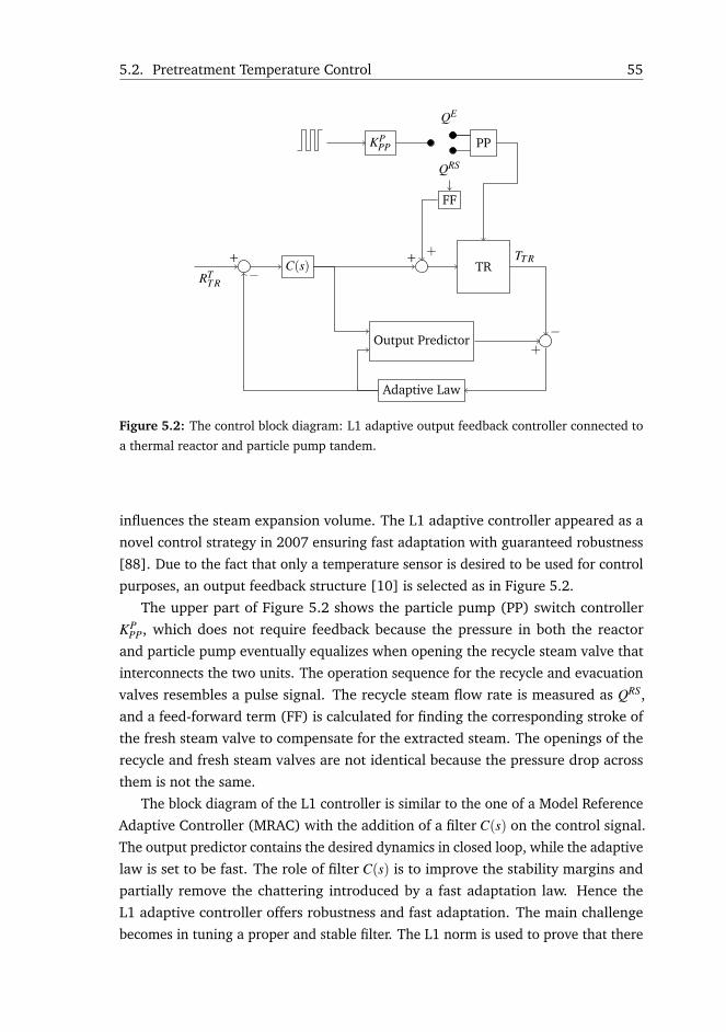
5.2. Pretreatment Temperature Control 55
C(s) TR
PP
RTT R
+ +
Output Predictor
Adaptive Law
TT R
−+
−
KPPP
QRS
QE
FF
+
Figure 5.2: The control block diagram: L1 adaptive output feedback controller connected to
a thermal reactor and particle pump tandem.
influences the steam expansion volume. The L1 adaptive controller appeared as a
novel control strategy in 2007 ensuring fast adaptation with guaranteed robustness
[88]. Due to the fact that only a temperature sensor is desired to be used for control
purposes, an output feedback structure [10] is selected as in Figure 5.2.
The upper part of Figure 5.2 shows the particle pump (PP) switch controller
KPPP, which does not require feedback because the pressure in both the reactor
and particle pump eventually equalizes when opening the recycle steam valve that
interconnects the two units. The operation sequence for the recycle and evacuation
valves resembles a pulse signal. The recycle steam flow rate is measured as QRS,
and a feed-forward term (FF) is calculated for finding the corresponding stroke of
the fresh steam valve to compensate for the extracted steam. The openings of the
recycle and fresh steam valves are not identical because the pressure drop across
them is not the same.
The block diagram of the L1 controller is similar to the one of a Model Reference
Adaptive Controller (MRAC) with the addition of a filter C(s) on the control signal.
The output predictor contains the desired dynamics in closed loop, while the adaptive
law is set to be fast. The role of filter C(s) is to improve the stability margins and
partially remove the chattering introduced by a fast adaptation law. Hence the
L1 adaptive controller offers robustness and fast adaptation. The main challenge
becomes in tuning a proper and stable filter. The L1 norm is used to prove that there
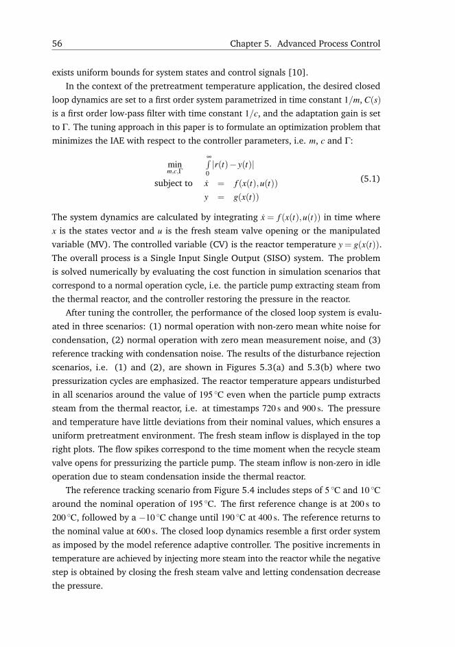
56 Chapter 5. Advanced Process Control
exists uniform bounds for system states and control signals [10].
In the context of the pretreatment temperature application, the desired closed
loop dynamics are set to a first order system parametrized in time constant 1/m, C(s)
is a first order low-pass filter with time constant 1/c, and the adaptation gain is set
to Γ. The tuning approach in this paper is to formulate an optimization problem that
minimizes the IAE with respect to the controller parameters, i.e. m, c and Γ:
minm,c,Γ
∞∫0|r(t)− y(t)|
subject to x = f (x(t),u(t))
y = g(x(t))
(5.1)
The system dynamics are calculated by integrating x = f (x(t),u(t)) in time where
x is the states vector and u is the fresh steam valve opening or the manipulated
variable (MV). The controlled variable (CV) is the reactor temperature y = g(x(t)).
The overall process is a Single Input Single Output (SISO) system. The problem
is solved numerically by evaluating the cost function in simulation scenarios that
correspond to a normal operation cycle, i.e. the particle pump extracting steam from
the thermal reactor, and the controller restoring the pressure in the reactor.
After tuning the controller, the performance of the closed loop system is evalu-
ated in three scenarios: (1) normal operation with non-zero mean white noise for
condensation, (2) normal operation with zero mean measurement noise, and (3)
reference tracking with condensation noise. The results of the disturbance rejection
scenarios, i.e. (1) and (2), are shown in Figures 5.3(a) and 5.3(b) where two
pressurization cycles are emphasized. The reactor temperature appears undisturbed
in all scenarios around the value of 195 ◦C even when the particle pump extracts
steam from the thermal reactor, i.e. at timestamps 720 s and 900 s. The pressure
and temperature have little deviations from their nominal values, which ensures a
uniform pretreatment environment. The fresh steam inflow is displayed in the top
right plots. The flow spikes correspond to the time moment when the recycle steam
valve opens for pressurizing the particle pump. The steam inflow is non-zero in idle
operation due to steam condensation inside the thermal reactor.
The reference tracking scenario from Figure 5.4 includes steps of 5 ◦C and 10 ◦Caround the nominal operation of 195 ◦C. The first reference change is at 200 s to
200 ◦C, followed by a −10 ◦C change until 190 ◦C at 400 s. The reference returns to
the nominal value at 600 s. The closed loop dynamics resemble a first order system
as imposed by the model reference adaptive controller. The positive increments in
temperature are achieved by injecting more steam into the reactor while the negative
step is obtained by closing the fresh steam valve and letting condensation decrease
the pressure.
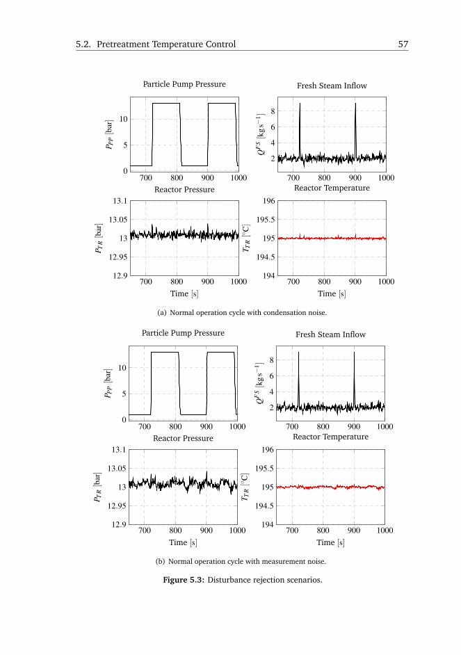
5.2. Pretreatment Temperature Control 57
700 800 900 10000
5
10P P
P[b
ar]
Particle Pump Pressure
700 800 900 1000
2
4
6
8
QF
S[k
gs−
1 ]
Fresh Steam Inflow
700 800 900 100012.9
12.95
13
13.05
13.1
Time [s]
P TR[b
ar]
Reactor Pressure
700 800 900 1000194
194.5
195
195.5
196
Time [s]
T TR[◦
C]
Reactor Temperature
(a) Normal operation cycle with condensation noise.
700 800 900 10000
5
10
P PP[b
ar]
Particle Pump Pressure
700 800 900 1000
2
4
6
8
QF
S[k
gs−
1 ]
Fresh Steam Inflow
700 800 900 100012.9
12.95
13
13.05
13.1
Time [s]
P TR[b
ar]
Reactor Pressure
700 800 900 1000194
194.5
195
195.5
196
Time [s]
T TR[◦
C]
Reactor Temperature
(b) Normal operation cycle with measurement noise.
Figure 5.3: Disturbance rejection scenarios.

58 Chapter 5. Advanced Process Control
0 200 400 600 8000.8
0.9
1
1.1
P PP[b
ar]
Particle Pump Pressure
0 200 400 600 8000
5
QF
S[k
gs−
1 ]
Fresh Steam Inflow
0 200 400 600 800
12
14
Time [s]
P TR[b
ar]
Reactor Pressure
0 200 400 600 800190
195
200
Time [s]
T TR[◦
C]
Reactor Temperature
Figure 5.4: Reference tracking with condensation noise.
The closed loop system performs satisfactory both in disturbance rejection by
reducing the reactor temperature variations, and in reference tracking ensuring
a fast change to a new temperature level. The controller setpoint is given by the
optimization layer designed in Chapter 4. More details about the adaptive controller
design including closed loop transfer function analysis can be read in Paper D.
5.3 Enzymatic pH Control
pH is another process key parameter because enzymes and yeast are highly
sensitive to the pH level following a Gaussian bell curve. A pH controller is requested
to keep the pH of the mixture at the optimal level, e.g. the peak of the enzymatic
activity curve. The enzymatic hydrolysis pH setpoint is taken from the enzymes
manufacturers, and remains constant throughout the entire process. In simultaneous
saccharification and fermentation an optimal pH profile exists as a trade-off between
enzymes and yeast optimal pH [89]. In this case, pH reference tracking is of interest.
The pH is disturbed by organic acids that are produced during pretreatment due
to hemicellulose removal, and also during enzymatic hydrolysis of the remaining
hemicellulose in the liquefaction tanks. In fermentation the pH is disturbed due
to CO2 production, and organic acids formation during saccharification of the
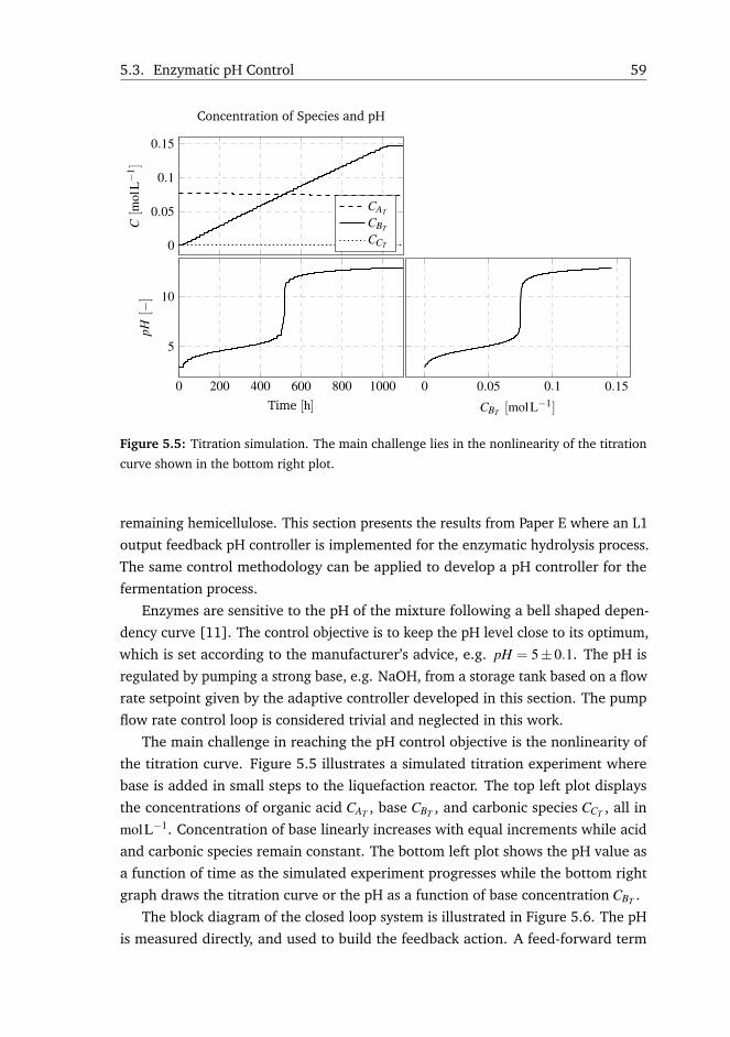
5.3. Enzymatic pH Control 59
0
0.05
0.1
0.15C[m
olL−
1 ]
Concentration of Species and pH
CAT
CBT
CCT
0 200 400 600 800 1000
5
10
Time [h]
pH[−
]
0 0.05 0.1 0.15
CBT [molL−1]
Figure 5.5: Titration simulation. The main challenge lies in the nonlinearity of the titration
curve shown in the bottom right plot.
remaining hemicellulose. This section presents the results from Paper E where an L1
output feedback pH controller is implemented for the enzymatic hydrolysis process.
The same control methodology can be applied to develop a pH controller for the
fermentation process.
Enzymes are sensitive to the pH of the mixture following a bell shaped depen-
dency curve [11]. The control objective is to keep the pH level close to its optimum,
which is set according to the manufacturer’s advice, e.g. pH = 5±0.1. The pH is
regulated by pumping a strong base, e.g. NaOH, from a storage tank based on a flow
rate setpoint given by the adaptive controller developed in this section. The pump
flow rate control loop is considered trivial and neglected in this work.
The main challenge in reaching the pH control objective is the nonlinearity of
the titration curve. Figure 5.5 illustrates a simulated titration experiment where
base is added in small steps to the liquefaction reactor. The top left plot displays
the concentrations of organic acid CAT , base CBT , and carbonic species CCT , all in
molL−1. Concentration of base linearly increases with equal increments while acid
and carbonic species remain constant. The bottom left plot shows the pH value as
a function of time as the simulated experiment progresses while the bottom right
graph draws the titration curve or the pH as a function of base concentration CBT .
The block diagram of the closed loop system is illustrated in Figure 5.6. The pH
is measured directly, and used to build the feedback action. A feed-forward term
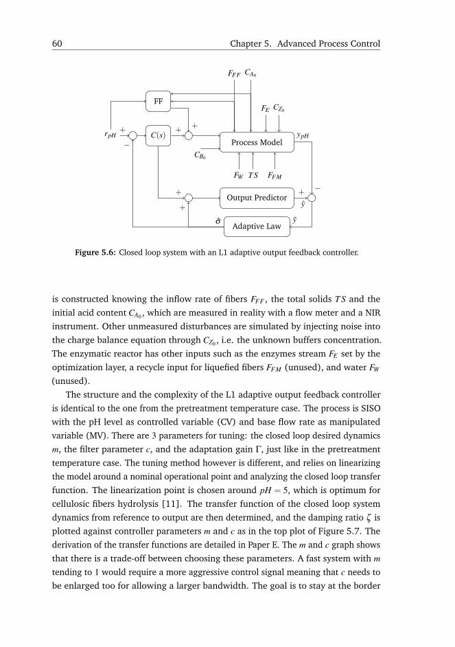
60 Chapter 5. Advanced Process Control
Process ModelCB0
FFF CA0
FE CZ0
FW T S FFM
C(s)+
FF
+rpH
+
Output Predictor
Adaptive Law
ypH
−+
y
y
+
σ
+
−
Figure 5.6: Closed loop system with an L1 adaptive output feedback controller.
is constructed knowing the inflow rate of fibers FFF , the total solids T S and the
initial acid content CA0 , which are measured in reality with a flow meter and a NIR
instrument. Other unmeasured disturbances are simulated by injecting noise into
the charge balance equation through CZ0 , i.e. the unknown buffers concentration.
The enzymatic reactor has other inputs such as the enzymes stream FE set by the
optimization layer, a recycle input for liquefied fibers FFM (unused), and water FW
(unused).
The structure and the complexity of the L1 adaptive output feedback controller
is identical to the one from the pretreatment temperature case. The process is SISO
with the pH level as controlled variable (CV) and base flow rate as manipulated
variable (MV). There are 3 parameters for tuning: the closed loop desired dynamics
m, the filter parameter c, and the adaptation gain Γ, just like in the pretreatment
temperature case. The tuning method however is different, and relies on linearizing
the model around a nominal operational point and analyzing the closed loop transfer
function. The linearization point is chosen around pH = 5, which is optimum for
cellulosic fibers hydrolysis [11]. The transfer function of the closed loop system
dynamics from reference to output are then determined, and the damping ratio ζ is
plotted against controller parameters m and c as in the top plot of Figure 5.7. The
derivation of the transfer functions are detailed in Paper E. The m and c graph shows
that there is a trade-off between choosing these parameters. A fast system with m
tending to 1 would require a more aggressive control signal meaning that c needs to
be enlarged too for allowing a larger bandwidth. The goal is to stay at the border
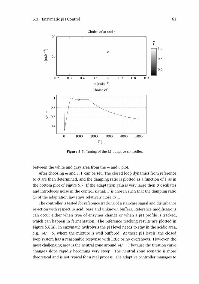
5.3. Enzymatic pH Control 61
0.2 0.3 0.4 0.5 0.6 0.7 0.8 0.9
50
100
m [rads−1]
c[r
ads−
1 ]
Choice of m and c
0.6
0.8
1.0
ζ
0 1000 2000 3000 4000 5000
0.4
0.6
0.8
1
Γ [−]
ζ Γ[−
]
Choice of Γ
Figure 5.7: Tuning of the L1 adaptive controller.
between the white and gray area from the m and c plot.
After choosing m and c, Γ can be set. The closed loop dynamics from reference
to σ are then determined, and the damping ratio is plotted as a function of Γ as in
the bottom plot of Figure 5.7. If the adaptation gain is very large then σ oscillates
and introduces noise in the control signal. Γ is chosen such that the damping ratio
ζΓ of the adaptation law stays relatively close to 1.
The controller is tested for reference tracking of a staircase signal and disturbance
rejection with respect to acid, base and unknown buffers. Reference modifications
can occur either when type of enzymes change or when a pH profile is tracked,
which can happen in fermentation. The reference tracking results are plotted in
Figure 5.8(a). In enzymatic hydrolysis the pH level needs to stay in the acidic area,
e.g. pH = 5, where the mixture is well buffered. At these pH levels, the closed
loop system has a reasonable response with little or no overshoots. However, the
most challenging area is the neutral zone around pH = 7 because the titration curve
changes slope rapidly becoming very steep. The neutral zone scenario is more
theoretical and is not typical for a real process. The adaptive controller manages to
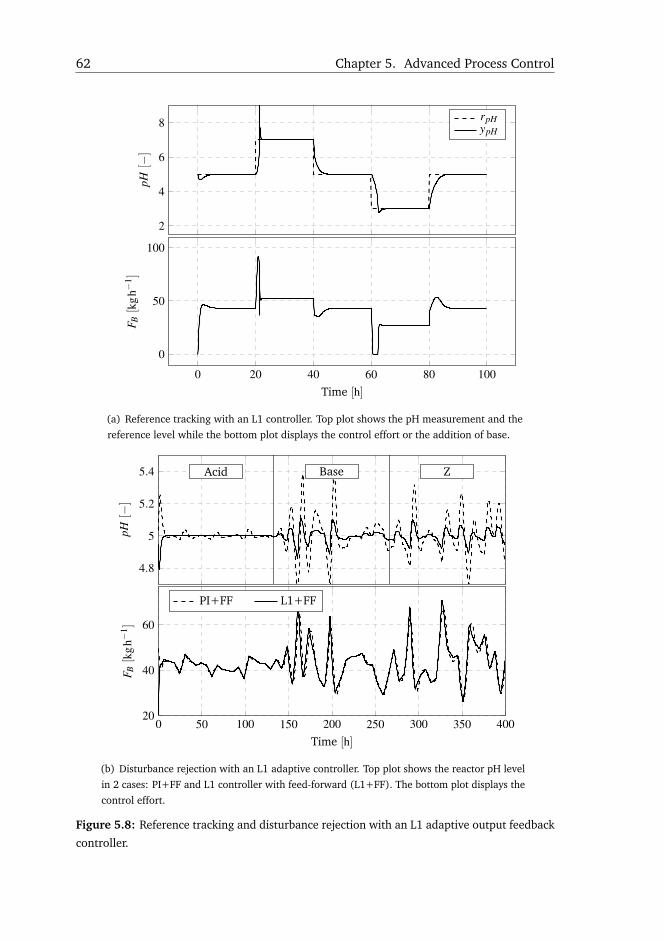
62 Chapter 5. Advanced Process Control
2
4
6
8
pH[−
]
rpHypH
0 20 40 60 80 100
0
50
100
Time [h]
F B[k
gh−
1 ]
(a) Reference tracking with an L1 controller. Top plot shows the pH measurement and thereference level while the bottom plot displays the control effort or the addition of base.
4.8
5
5.2
5.4 Acid Base Z
pH[−
]
0 50 100 150 200 250 300 350 40020
40
60
Time [h]
F B[k
gh−
1 ]
PI+FF L1+FF
(b) Disturbance rejection with an L1 adaptive controller. Top plot shows the reactor pH levelin 2 cases: PI+FF and L1 controller with feed-forward (L1+FF). The bottom plot displays thecontrol effort.
Figure 5.8: Reference tracking and disturbance rejection with an L1 adaptive output feedback
controller.

5.4. Optimal Feed Rate Profile for Glucose Fermentation 63
stabilize the process at pH = 7 with a large overshoot but converges eventually. As
the system is very fast around the neutral zone, a faster adaptation law might be
required in order to reduce the overshoot.
The disturbance rejection scenario is shown in Figure 5.8(b), and comprises
of three zones: acid, base and unknown buffers Z. Each source of disturbance is
enabled only in the designated area. The L1 adaptive controller is compared against
a classical Proportional Integral (PI) controller that was tuned using the Skogestad
internal model approach for PID tuning [90]. The feed-forward term is enabled
for both controllers. The adaptive scheme is not necessarily more aggressive as
its control effort is similar to the classical controller but reacts sooner than the PI.
Disturbances are successfully rejected in all cases ensuring little deviations from the
optimal pH level within a band of ±0.1 units.
5.4 Optimal Feed Rate Profile for Glucose Fermentation
Figure 4.3(b) from the optimization section showed that fermentation costs
can be high in biorefinery operation. The objective of this part of the study is to
determine an optimal feed rate profile for liquefied fibers such that the amount of
yeast is minimized while achieving glucose depletion in approximately the same
amount of time as in a classical operation with a constant feed rate. The results
from this section have been developed in collaboration with the Automatic Control
Laboratory from École Polytechnique Fédérale de Lausanne (EPFL). A commercial
scale fermentation tank can reach a volume of 250 m3 requiring the fed-batch phase
to take 40 h to 60 h to reach the desired hold-up, time when reactions already take
place. Plants following a traditional operation fill the fermentation reactors with a
constant feed rate. Such a strategy can lead to an early accumulation of inhibitors
and sugars that delay the reactions. In order to compensate the inhibition, more
yeast would be required, which attracts higher costs.
The two strategies are conceptually illustrated in Figure 5.9. The constant feed
(a) Constant feed rate. (b) Variable feed rate.
Figure 5.9: Constant and variable feed rates.
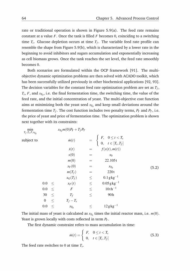
64 Chapter 5. Advanced Process Control
rate or traditional operation is shown in Figure 5.9(a). The feed rate remains
constant at a value F . Once the tank is filled F becomes 0, coinciding to a switching
time Ts. Glucose depletion occurs at time Tf . The variable feed rate profile can
resemble the shape from Figure 5.9(b), which is characterized by a lower rate in the
beginning to avoid inhibitors and sugars accumulation and exponentially increasing
as cell biomass grows. Once the tank reaches the set level, the feed rate smoothly
becomes 0.
Both scenarios are formulated within the OCP framework [91]. The multi-
objective dynamic optimization problems are then solved with ACADO toolkit, which
has been successfully utilized previously in other biochemical applications [92, 93].
The decision variables for the constant feed rate optimization problem are set as Tf ,
Ts, F, and xY0 , i.e. the final fermentation time, the switching time, the value of the
feed rate, and the initial concentration of yeast. The multi-objective cost function
aims at minimizing both the yeast seed xY0 and keep small deviations around the
fermentation time Tf . The cost function includes two penalty terms, PY and PT , i.e.
the price of yeast and price of fermentation time. The optimization problem is shown
next together with its constraints:
minTf ,Ts,F,xY0
xY0m(0)PY +Tf PT
subject to m(t) =
{F, 0≤ t < Ts
0, t ∈ [Ts,Tf ]
x(t) = f (x(t),m(t))
x(0) = x0
m(0) = 22.105txY (0) = xY0
m(Tf ) = 220txG(Tf ) ≤ 0.1gkg−1
0.0 ≤ xF(t) ≤ 0.05gkg−1
0.0 ≤ F ≤ 10th−1
30 ≤ Tf ≤ 90h0 ≤ Tf −Ts
0.0 ≤ xY0 ≤ 12gkg−1
(5.2)
The initial mass of yeast is calculated as xY0 times the initial reactor mass, i.e. m(0).Yeast is grown locally with costs reflected in term PY .
The first dynamic constraint refers to mass accumulation in time:
m(t) =
{F, 0≤ t < Ts
0, t ∈ [Ts,Tf ](5.3)
The feed rate switches to 0 at time Ts.

5.4. Optimal Feed Rate Profile for Glucose Fermentation 65
The second dynamic constraint refers to the fermentation reactor kinetics, which
were presented in Chapter 3:
x(t) = f (x(t),m(t),F) (5.4)
where x symbolizes the species concentrations, and m is the reactor hold-up.
The initial conditions constraints consists of: the fiber concentrations when the
fed-batch phase starts, i.e. x(0) = x0, initial reactor mass m(0) = 22.105t, and yeast
seed xY (0) = xY0 . The final time constraints refer to reactor fill limit m(Tf ) = 220t,and glucose depletion xG(Tf )≤ 0.1gkg−1. Accumulation of inhibitors at any given
time is limited by xF(t) ≤ 0.05gkg−1. Additional bounds are set for all decision
variables.
The optimization control problem for variable feed profile is formulated below:
minF(t),Tf ,xY0
xY0m0PY +Tf PT
subject to x(t) = f (x(t),F(t))
x(0) = x0
m(0) = 22.105tm(Tf ) = 220txY (0) = xY0
xG(Tf ) ≤ 0.1gkg−1
0.0 ≤ xF(t) ≤ 0.05gkg−1
0.0 ≤ F(t) ≤ 10th−1
30 ≤ Tf ≤ 90h0.0 ≤ xY0 ≤ 12gkg−1
(5.5)
The problem is similar to OCP (5.2) except that the decision variable F(t) becomes
a function of time and switching time Ts is removed. The cost function and the
constraints are identical.
The results of the two strategies are compared in Figure 5.10. The mass and the
feed rates are illustrated in Figure 5.10(a). The constant inflow of liquefied fibers is
set to approximately 3.85 th−1 and fills the reactor in about 57 h. The variable feed
rate starts at a lower level than in the constant feed case but gradually increases as
time passes until it reaches a peak of 9 th−1 around 40 h. In the next 5 h the feed rate
decreases fast until it reaches 0 th−1. The tank is filled faster than in the constant
rate case by about 12 h.
The reactor kinetics are shown in Figure 5.10(b). The constant feed rate is
limited by the inhibitors accumulation constraints, which is reached in the first 3 has shown in the top plot. In the feed profile case, the flow rate allows accumulation
of inhibitors near the constraint limit. The system does not operate exactly at the
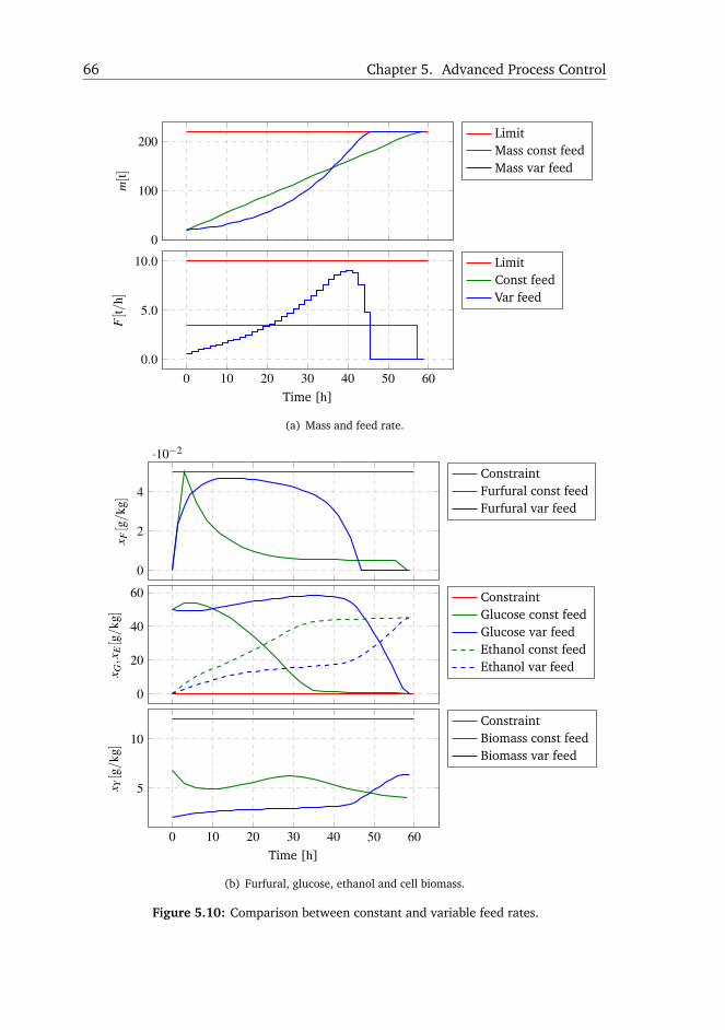
66 Chapter 5. Advanced Process Control
0
100
200
m[t]
LimitMass const feedMass var feed
0 10 20 30 40 50 600.0
5.0
10.0
Time [h]
F[t/
h]
LimitConst feedVar feed
(a) Mass and feed rate.
0
2
4
·10−2
x F[g/k
g]
ConstraintFurfural const feedFurfural var feed
0
20
40
60
x G,x
E[g/k
g]
ConstraintGlucose const feedGlucose var feedEthanol const feedEthanol var feed
0 10 20 30 40 50 60
5
10
Time [h]
x Y[g/
kg]
ConstraintBiomass const feedBiomass var feed
(b) Furfural, glucose, ethanol and cell biomass.
Figure 5.10: Comparison between constant and variable feed rates.
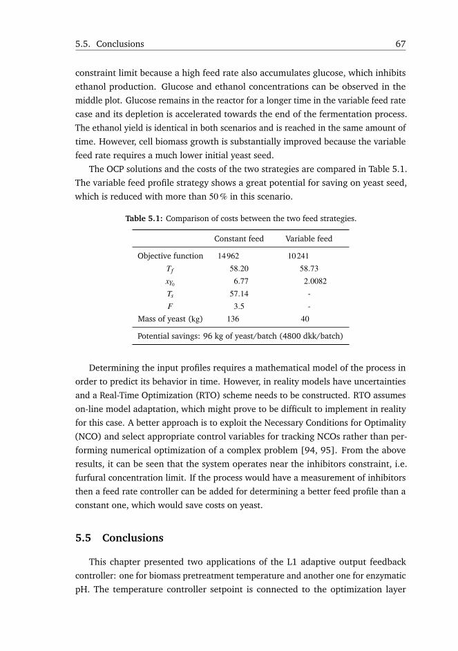
5.5. Conclusions 67
constraint limit because a high feed rate also accumulates glucose, which inhibits
ethanol production. Glucose and ethanol concentrations can be observed in the
middle plot. Glucose remains in the reactor for a longer time in the variable feed rate
case and its depletion is accelerated towards the end of the fermentation process.
The ethanol yield is identical in both scenarios and is reached in the same amount of
time. However, cell biomass growth is substantially improved because the variable
feed rate requires a much lower initial yeast seed.
The OCP solutions and the costs of the two strategies are compared in Table 5.1.
The variable feed profile strategy shows a great potential for saving on yeast seed,
which is reduced with more than 50 % in this scenario.
Table 5.1: Comparison of costs between the two feed strategies.
Constant feed Variable feed
Objective function 14962 10241
Tf 58.20 58.73
xY0 6.77 2.0082
Ts 57.14 -
F 3.5 -
Mass of yeast (kg) 136 40
Potential savings: 96 kg of yeast/batch (4800 dkk/batch)
Determining the input profiles requires a mathematical model of the process in
order to predict its behavior in time. However, in reality models have uncertainties
and a Real-Time Optimization (RTO) scheme needs to be constructed. RTO assumes
on-line model adaptation, which might prove to be difficult to implement in reality
for this case. A better approach is to exploit the Necessary Conditions for Optimality
(NCO) and select appropriate control variables for tracking NCOs rather than per-
forming numerical optimization of a complex problem [94, 95]. From the above
results, it can be seen that the system operates near the inhibitors constraint, i.e.
furfural concentration limit. If the process would have a measurement of inhibitors
then a feed rate controller can be added for determining a better feed profile than a
constant one, which would save costs on yeast.
5.5 Conclusions
This chapter presented two applications of the L1 adaptive output feedback
controller: one for biomass pretreatment temperature and another one for enzymatic
pH. The temperature controller setpoint is connected to the optimization layer

68 Chapter 5. Advanced Process Control
developed in the previous chapter, while the pH controller ensures the efficiency of
the enzymatic activity. The main presented novelties came from the tuning methods
of these controllers: one based on closed loop transfer function analysis, and another
one based on formulating an optimization problem.
The adaptive controllers were followed by an optimal controller for determining
the feed rate profile in glucose fermentation. These results showed that there is
a high potential in yeast economy that can be achieved with a variable feed rate
profile. Further investigation is required in order to transform the simulation results
into an implementable RTO scheme.

Chapter 6
Conclusions and Future Research
6.1 Summary of Conclusions
The core contribution of this research is a complex dynamic model library suit-
able for industrial size plants. Other parts of this work include model-based tools
that improve the operation of large scale biorefineries: an optimization layer for
maximizing the economical profit of the biorefinery, and an advanced control layer
to support an optimal operation.
The dynamic model library captured in great detail and accurately the behavior of
the key steps in biomass conversion, i.e. hydrothermal pretreatment with steam and
enzymatic hydrolysis. The library was completed with co-fermentation supported by
GMO yeast. The models from this work were subject to a comprehensive analysis
methodology for validation, and for assessing their sensitivity and uncertainty. This
work published for the first time validation against demonstration scale real data,
which proves that the model library is ready to be used in real industrial applications.
The models were then exploited to optimize the biorefinery operation for max-
imizing its economical profit. The plant was treated in an integrated manner in
order to capture the trade-offs between the biomass conversion steps. Too little pre-
treatment might not open the biomass sufficiently leading to an increase in enzyme
dosage and yeast seed while an over pretreatment lead to inhibitors formation that
decrease the ethanol yield in fermentation. The optimization layer identifies the best
compromise, and offers setpoints for the key process parameters, i.e. thermal reactor
temperature, enzyme dosage and yeast seed. The optimization part of the study was
carried in a simulated environment and showed potential economical improvements
of 18 % over a traditional plant operation.
The optimization layer is supported by an advanced automation and control
layer. Pretreatment temperature and pH in enzymatic hydrolysis are key parameters

70 Chapter 6. Conclusions and Future Research
of the biorefinering process. Two high performance L1 adaptive controllers were
developed: one for pretreatment temperature and another one for pH in enzymatic
hydrolysis. The L1 adaptive controller for the thermal reactor temperature ensured
little deviations from the setpoint when the particle pump extracted steam for
pressurization of biomass. Changes in setpoints as indicated by the optimization layer
can also be performed with a reasonable fast first order response. The enzymatic
pH posed a higher challenge due to its nonlinear titration curve. Once again the
L1 adaptive controller was capable of minimizing deviations around the setpoint
ensuring an efficient enzymatic activity. The L1 adaptive controllers were tuned
systematically: by formulating an optimization problem that minimizes the IAE, and
by analyzing closed loop transfer functions for obtaining a specific performance.
The last component added to the control layer was an optimum feed rate profile
of liquefied fibers to fermentation. The challenge was to avoid accumulation of
inhibitors and sugars that could delay reactions and decrease ethanol yield. The
results showed an important reduction in yeast amount for obtaining the same
ethanol yield.
6.2 Future Research
There is great potential for future research in the area of biorefinery automation.
The advanced control and optimization tools formulated in this work offer a higher
profitability to the Inbicon technology making it more attractive to customers. As fu-
ture perspectives, emphasis will be placed on implementation on real-time hardware
making all these tools part of the commercial Inbicon technology. The modeling
work is continuous and will be maintained and updated with newly documented
phenomena, as well as validated against more real data.
Simultaneous saccharification and fermentation can be further improved. The
method used for determining the optimal feed rate profile can be extended for
pH and temperature because enzymes and yeast do not have the same optimal
conditions. This would lead to an optimal economic operation of the fermentation
process that would save even more costs.
The optimization work showed great potential and should be extended with
real-time optimization for implementation possibly following NCO tracking methods.
The dynamic models can also be transformed into soft sensors and state observers
such that the refinery operators can monitor all variables of interest even in the
absence of a real measurement. Faults happen in reality and detection and isolation
are important for an efficient operation. A model-based diagnosis layer would add
even further value to the Inbicon technology.
Paper A
Dynamic Modeling andValidation of a BiomassHydrothermal PretreatmentProcess - A Demonstration ScaleStudyRemus Mihail Prunescu1, Mogens Blanke1, Jon Geest Jakobsen2, Gürkan Sin*3
1Department of Electrical Engineering, Automation and Control Group, Technical
University of Denmark, Elektrovej Building 326, 2800, Kgs. Lyngby, Denmark
2Department of Process Control and Optimization, DONG Energy Thermal Power
A/S, Nesa Allé 1, 2820, Gentofte, Denmark
3CAPEC-PROCESS, Department of Chemical and Biochemical Engineering, Technical
University of Denmark, Søltofts Plads Buildings 227 and 229, 2800, Kgs. Lyngby,
Denmark
Abstract:
Hydrothermal pretreatment of lignocellulosic biomass is a cost effective technology
for second generation biorefineries. The process occurs in large horizontal and
pressurized thermal reactors where the biomatrix is opened under the action of
steam pressure and temperature to expose cellulose for the enzymatic hydrolysis
process. Several by-products are also formed, which disturb and act as inhibitors
downstream. The objective of this study is to formulate and validate a large scale
hydrothermal pretreatment dynamic model based on mass and energy balances,
together with a complex conversion mechanism and kinetics. The study includes
a comprehensive sensitivity and uncertainty analysis, with parameter estimation
from real-data in the 178 ◦C to 185 ◦C range. To highlight the application utility of
the model, a state estimator for biomass composition is developed. The predictions
capture well the dynamic trends of the process, outlining the value of the model for
simulation, control design, and optimization for full-scale applications.
*Principal corresponding author. Tel.: +45 45252806; E-mail: [email protected]
72 Paper A. Pretreatment Modeling
A.1 Introduction
Lignocellulosic biomass, e.g. wheat straw, corn stover, bagasse etc, consist of
cellulose, hemicellulose, lignin, ash, and a negligible amount of residues [37]. The
cellulosic fibers contain glucose units, which are necessary for biofuel production, but
layers of hemicellulose and lignin make cellulose hardly accessible. The goal of the
pretreatment process is to relocate lignin, and partially hydrolyze the hemicellulose,
which opens the biomatrix for cellulose such that enzymes can easily access it in the
enzymatic hydrolysis process downstream [40].
Chiaramonti et al. [44] review various methods of pretreatment, e.g. autohydrol-
ysis, steam explosion, acid hydrolysis, alkaline hydrolysis, and many others. Studies
show that hydrothermal pretreatment with steam excels in cost effectiveness and,
therefore, has been commercialized in large scale second generation biorefineries.
Integrating the biorefinery with a power plant following the Integration Biomass
Utilization System (IBUS) also contributes to reducing costs [4]. The pretreatment
process partially depolymerizes hemicellulose creating several degradation and by-
products, i.e. organic acids, xylooligomers, xylose, and inhibitors, e.g. furfural and
5-HMF, which impact the downstream processes. The organic acids, i.e. acetic,
succinic and lactic acid influence the pH of pretreated fibers and become an issue
in the enzymatic hydrolysis process [6]. Xylooligomers and xylose act as strong
inhibitors of cellulose hydrolysis by enzymes [51], while furfural and 5-HMF inhibit
the fermentation process [52]. Also carbohydrates react with degradation products
such as furfural to create spherical droplets with lignin like structure named pseudo-
lignin, which can degrade the enzymatic activity [53]. Experimental studies show
that reactor temperature and retention time relate to biomass conversion [50].
Lavarack et al. [73] formulate a mechanistic acid hydrolysis model capable of
predicting cellulose, xylan and furfural concentrations but no one evaluated the
model for steam pretreatment, and at a large scale. This model has been used in
later studies for model-based optimization of bioprocesses under uncertainty [9] and
biorefinery configurations [96]. Overend et al. [97] present an empirical modeling
alternative known as the severity factor, which Petersen et al. [50] validated in
laboratory experiments for xylan recovery and furfural formation. These models
are incomplete because: (1) they miss production of important by-products such as
organic acids, xylooligomers, and pseudo-lignin; and (2) assume a uniform thermal
environment, which is not the case in a full scale reactor [71]. This study extends
the existing Lavarack et al. [73] model to demonstration scale using computational
fluid dynamics techniques, taking into account temperature variations in a large
scale thermal reactor, and production of the above enumerated by-products. The
A.2. Methods 73
model is then calibrated and validated against real data that were logged throughout
several hours of operation at a demonstration scale facility.
This study also assesses the model reliability through a comprehensive sensitivity
and uncertainty analysis. The sensitivity analysis quantifies the importance of each
model parameter and creates an identifiable subset of parameters that is used for
parameter estimation following the methodology from Sin et al. [8] and Prunescu
and Sin [6].
Samples of fibers were collected after the pretreatment process and were ana-
lyzed with near infra-red instruments (NIR) to determine their composition. The
model parameters are estimated using the NIR readings. The uncertainty analysis
determines a confidence interval for model predictions and is carried with respect to
both model and feed parameters following the method from Sin et al. [8]. As a global
sensitivity measure, the standardized regression coefficients (SRC) are computed
in order to identify the model parameters responsible for most of the variations in
model predictions [66]. A residual analysis follows to identify how much of the
signal is represented by the model. The study ends with a model application as a
state estimator by using a static Kalman filter. The state estimator not only filters the
NIR measurements but also predicts by-products formation such as C5 sugars and
inhibitors.
This study has the following structure: the Methods section gives an overview
of a state of the art demonstration scale biorefinery from where the real measure-
ments were collected; a Model Development section follows, which formulates the
mathematical model for the pretreatment process along with the model analysis
methodology; the Results and Discussion section presents the model analysis and
validation results, and the model application as a state estimator; the study ends
with a Conclusions section, which summarizes all findings.
A.2 Methods
A.2.1 Biorefinery Experimental Setup
Figure A.1 shows an overview of a demonstration scale second generation
bioethanol plant. Biomass is first pretreated in a continuous thermal reactor where
the temperature can be set within 160 ◦C to 210 ◦C, and the retention time can be
adjusted from 6 min to 20 min. Following the IBUS concept, a nearby power plant
supplies the biorefinery with steam for pressurizing the thermal reactor, thus reach-
ing the necessary reaction temperatures. The steam supply pipe provides saturated
steam at 18×105 Pa. After the thermal reactor, the pretreated slurry is first washed
and then the liquid part is separated from fibers in a screw press. The liquid part is

74 Paper A. Pretreatment Modeling
Figure A.1: Process flow diagram for a second generation biorefinery: pretreatment, enzy-
matic hydrolysis, C5 and C6 co-fermentation, and purification. The samples for NIR analysis
are extracted after the pretreatment process every 10 min. The thermal reactor is monitored
with two temperature sensors: one at the top and another one at the bottom of the reactor.
rich in C5 sugars, i.e. xylooligomers, xylose and arabinose, as a result of partially
hydrolyzing the hemicellulose in the thermal reactor.
The cellulosic fibers are transported on a conveyor belt to the enzymatic hy-
drolysis tank. Enzymes are added in the liquefaction tank where cellulose and the
remaining xylan are converted to glucose and xylose. The enzymatic hydrolysis
process has been detailed and analyzed in Prunescu and Sin [6]. The C5 and C6
sugars are then co-fermented for ethanol production in scheduled batch reactors
with genetically modified organisms (GMOs) for enhancing bioethanol production.
The purification and separation phase contains two distillation columns and
molecular sieves. Lignin is separated in the first distillation column, while ethanol is
purified to 99.5 % in the second column and in the molecular sieves. The recovered
lignin is transported to an evaporation plant and solidified as bio-pellets, which are
sent to the nearby power plant for burning.
There is a timeline indicator at the bottom of Figure A.1 showing the retention
time for each section of the biorefinery. The pretreatment process and distillation are
the fastest processes with a duration of maximum half an hour, while the enzymatic
hydrolysis and fermentation can last 5 to 7 days each.
The demonstration scale facility has a processing capacity of 4000 kgh−1 of
biomass [3]. Samples of pretreated fibers were extracted after the pretreatment
process every 10 min for a total duration of 15 h. The samples were then analyzed

A.2. Methods 75
with near infra-red instruments (NIR) to determine their composition with respect to
cellulose, xylan, lignin, acetic acid, and furfural. The thermal reactor was monitored
with two temperature sensors, one placed at the top of the tank for measuring the
temperature in the steam layer, and another one placed at the bottom of the reactor
to measure the biomass temperature.
A.2.2 Dataset
Figure A.2 shows the raw temperature and NIR measurements collected through-
out the 15 h of operation. The dataset is split in two subsets: one is used for
estimation purposes, while the other for validation. The estimation dataset is identi-
fied in all figures with a grey background. The top reactor temperature oscillates
within 180 ◦C to 190 ◦C due to the pressurization unit, which takes the biomass from
atmospheric to reactor pressure with recycled steam from the reactor. The whole
process is thoroughly explained in Prunescu et al. [71]. There is a temperature
difference between the top and bottom of the reactor due to the insulation properties
of the biomass, and also because vertical mixing in the reactor was not possible due
to a low horizontal pushing speed.
A.2.3 Model Analysis Methodology
The model analysis follows the methodology from Table A.1:
1. The first step is to calibrate the model considering the entire set of parameters.
Ideally, this system identification exercise should give the set of parameters
that has the smallest sum of squared errors between model predicted output
and actual measurements. In the present case, this is a nonlinear least squares
problem and local minima can be obstacles. The parameter estimation may be
solved in Matlab with the fminsearch function, coupled with a cost function
that calculates the prediction error, if the initial parameter guess is sufficiently
close to a global minimum.
2. The second step is to investigate which parameters of the model could be
determined given the input and the model structure [63]. This selection is
achieved through assessment of sensitivity of the partial derivatives of the
cost function with respect to each model parameter. After computing the
sensitivities, δ msqr, all parameters are ranked with respect to their value of
δ msqr. Parameters that have low sensitivity are more uncertain that those with
high sensitivity and would not contribute to model accuracy. Therefore, a
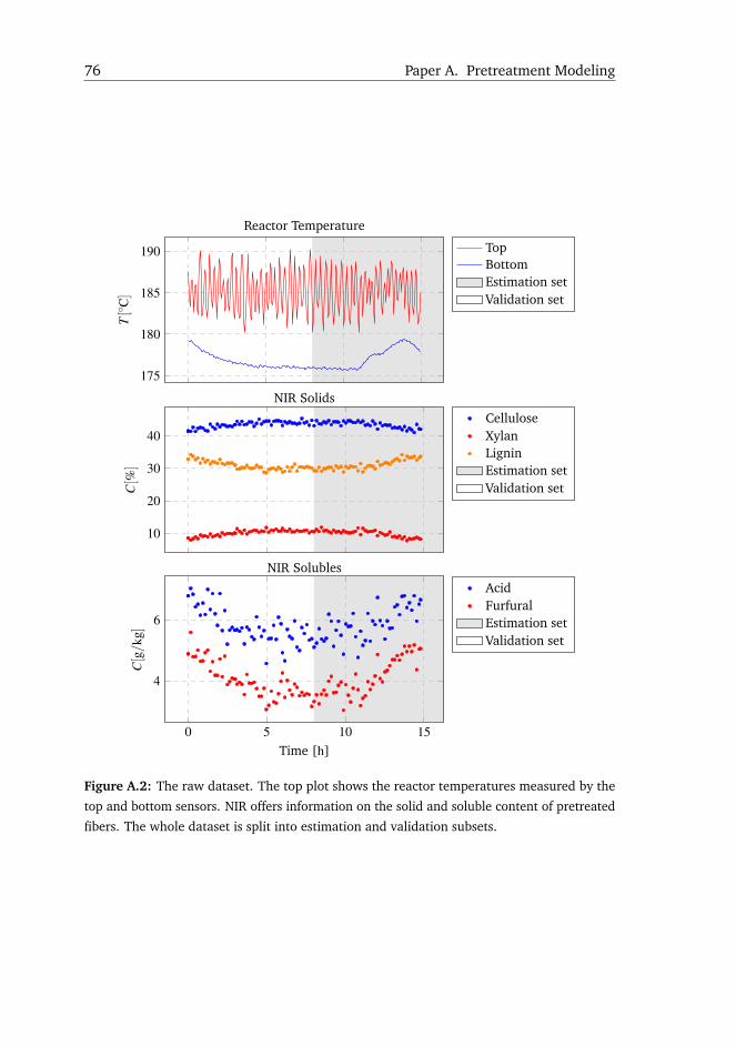
76 Paper A. Pretreatment Modeling
175
180
185
190
T[◦
C]
Reactor Temperature
TopBottomEstimation setValidation set
10
20
30
40
C[%
]
NIR Solids
CelluloseXylanLigninEstimation setValidation set
0 5 10 15
4
6
Time [h]
C[g/k
g]
NIR Solubles
AcidFurfuralEstimation setValidation set
Figure A.2: The raw dataset. The top plot shows the reactor temperatures measured by the
top and bottom sensors. NIR offers information on the solid and soluble content of pretreated
fibers. The whole dataset is split into estimation and validation subsets.
A.3. Model Development 77
relevant subset of parameters is selected based on δ msqr being higher than a
threshold.
3. In the third step the reduced set of parameters is identified using the NIR
measurements from the demonstration scale plant. The correlation matrix and
standard deviations of the estimates are also computed.
4. This step quantifies the prediction uncertainty. Having the covariance matrix
and standard deviations from the previous step allows Latin Hypercube Sam-
pling (LHS) [65] with correlation control. The feed parameters is another
source of uncertainty and is included in this analysis. N Monte Carlo simu-
lations are then run with sampled values and the 5th-95th percentiles of the
model predictions are found. A global sensitivity analysis follows by fitting
a linear model from parameters to model predictions and the standardized
regression coefficients are computed to identify which parameters are the most
important for explaining the output uncertainty.
5. The model estimation error or the residuals are analyzed in this step. A
simulation is run with the estimated parameters using the entire set of data
(not only the estimation set). The residuals distribution and autocorrelation
are calculated in order to assess the quality of model predictions. A good
model captures most of the signal in measurements and is characterized by
residuals being Gaussian with uncorrelated increments.
A.3 Model Development
The mathematical model consists of mass and energy balances for the pretreat-
ment process. In large scale plants, the most common continuous thermal reactor
is a long tank with cylindrical shape. This study employs simplified computational
fluid dynamics tools for modeling the composition and temperature profiles.
A.3.1 Mass Balance
The thermal reactor has a continuous operation and the mass balance is estab-
lished as the accumulation of mass per unit of time equals the difference between
inflow and outflow rates:dMdt
= Fin−Fout (A.1)
where M is the total mass of biomass inside the reactor, Fin is the inflow rate of
pressurized biomass and Fout is the outflow rate of pretreated biomass.
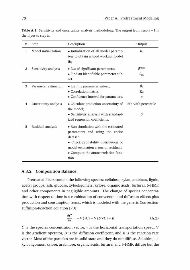
78 Paper A. Pretreatment Modeling
Table A.1: Sensitivity and uncertainty analysis methodology. The output from step k−1 is
the input to step k.
# Step Description Output
1 Model initialization • Initialization of all model parame-
ters to obtain a good working model
fit;
θ0
2 Sensitivity analysis • List of significant parameters; δ msqr
• Find an identifiable parameter sub-
set.
θR0
3 Parameter estimation • Identify parameter subset; θR
• Correlation matrix; Rθ
• Confidence interval for parameters. σ
4 Uncertainty analysis • Calculate prediction uncertainty of
the model;
5th-95th percentile
• Sensitivity analysis with standard-
ized regression coefficients.
β
5 Residual analysis • Run simulation with the estimated
parameters and using the entire
dataset
• Check probability distribution of
model estimation errors or residuals
• Compute the autocorrelation func-
tion
A.3.2 Composition Balance
Pretreated fibers contain the following species: cellulose, xylan, arabinan, lignin,
acetyl groups, ash, glucose, xylooligomers, xylose, organic acids, furfural, 5-HMF,
and other components in negligible amounts. The change of species concentra-
tion with respect to time is a combination of convection and diffusion effects plus
production and consumption terms, which is modeled with the generic Convection-
Diffusion-Reaction equation [70]:
∂C∂ t
=−∇(vC)+∇(D∇C)+R (A.2)
C is the species concentration vector, v is the horizontal transportation speed, ∇is the gradient operator, D is the diffusion coefficient, and R is the reaction rate
vector. Most of the particles are in solid state and they do not diffuse. Solubles, i.e.
xylooligomers, xylose, arabinose, organic acids, furfural and 5-HMF, diffuse but the
A.3. Model Development 79
snail pushing the biomass along the reactor separates the tank in chambers due to
its pallets, which leads to little exchange of matter between these chambers. If the
reactor is split in the same number as the chambers created by the rotational snail
pallets then the diffusion coefficient can be dropped:
∂C∂ t
=−∇(vC)+R (A.3)
The horizontal speed v is set to a constant value such that to meet a certain
retention time:
v =Lr
tr(A.4)
where Lr is the reactor length and tr is the retention time. E.g., a thermal reactor of
12 m with a retention time set to 15 min has a horizontal speed of 0.013 ms−1, which
is a low speed not capable of agitating the biomass vertically.
Since the reactor tank is longer on one axis, the partial derivatives with respect
to the other axis could be dropped. It is assumed that the biomass composition
changes only along the reactor and remains uniform in the other directions:
∂C∂ t
=−vdCdz
+R (A.5)
where z is the axis oriented along the reactor from inlet to outlet. Due to the low
horizontal speed, the vertical uniformity assumption stands valid only if the biomass
level in the reactor is low. At high biomass levels, the temperature gradient causes
different pretreatment layers and the reactor needs to be split on the vertical axis
too [71]. The data in this study was collected at low reactor levels and vertical
uniformity can be assumed but differences between the steam and biomass layer
temperatures still exist.
Figure A.3 illustrates the concept of splitting a reactor tank of length Lr into N
smaller reactors, or cells, of width δz. Equation A.5 is then discretized in space using
a Upwind Difference Scheme (UDS), which is a more stable technique for moving
environments [72]:dCk
dt=
uz
δz(Ck−1−Ck)+Rk (A.6)
Ck is the composition vector in central cell k, Ck−1 is the composition vector from the
western neighbor, and Rk is the reaction rate vector from current cell k. Movement
from west to east (left to right) is assumed. The composition vector will be detailed
in the next section.
A.3.3 Mechanistic Modeling for Hydrothermal Mediated Pretreatment
Raw biomass consists of cellulose, hemicellulose (arabinan and xylan), lignin,
acetyl groups, ash, water, and other components in negligible amounts. Table A.2
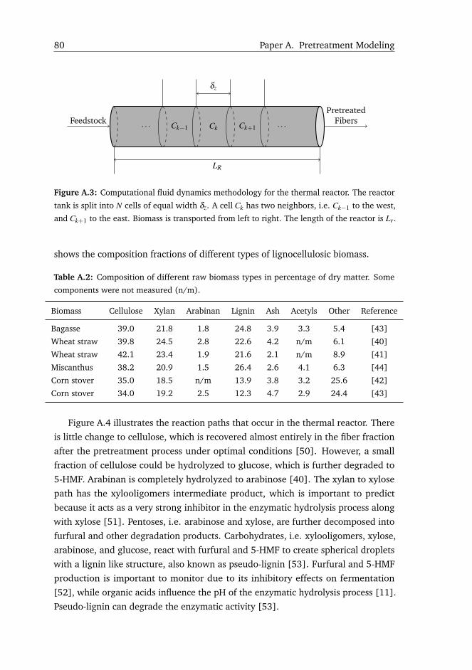
80 Paper A. Pretreatment Modeling
LR
Ck Ck+1Ck−1. . . . . .
δz
FeedstockPretreated
Fibers
Figure A.3: Computational fluid dynamics methodology for the thermal reactor. The reactor
tank is split into N cells of equal width δz. A cell Ck has two neighbors, i.e. Ck−1 to the west,
and Ck+1 to the east. Biomass is transported from left to right. The length of the reactor is Lr.
shows the composition fractions of different types of lignocellulosic biomass.
Table A.2: Composition of different raw biomass types in percentage of dry matter. Some
components were not measured (n/m).
Biomass Cellulose Xylan Arabinan Lignin Ash Acetyls Other Reference
Bagasse 39.0 21.8 1.8 24.8 3.9 3.3 5.4 [43]
Wheat straw 39.8 24.5 2.8 22.6 4.2 n/m 6.1 [40]
Wheat straw 42.1 23.4 1.9 21.6 2.1 n/m 8.9 [41]
Miscanthus 38.2 20.9 1.5 26.4 2.6 4.1 6.3 [44]
Corn stover 35.0 18.5 n/m 13.9 3.8 3.2 25.6 [42]
Corn stover 34.0 19.2 2.5 12.3 4.7 2.9 24.4 [43]
Figure A.4 illustrates the reaction paths that occur in the thermal reactor. There
is little change to cellulose, which is recovered almost entirely in the fiber fraction
after the pretreatment process under optimal conditions [50]. However, a small
fraction of cellulose could be hydrolyzed to glucose, which is further degraded to
5-HMF. Arabinan is completely hydrolyzed to arabinose [40]. The xylan to xylose
path has the xylooligomers intermediate product, which is important to predict
because it acts as a very strong inhibitor in the enzymatic hydrolysis process along
with xylose [51]. Pentoses, i.e. arabinose and xylose, are further decomposed into
furfural and other degradation products. Carbohydrates, i.e. xylooligomers, xylose,
arabinose, and glucose, react with furfural and 5-HMF to create spherical droplets
with a lignin like structure, also known as pseudo-lignin [53]. Furfural and 5-HMF
production is important to monitor due to its inhibitory effects on fermentation
[52], while organic acids influence the pH of the enzymatic hydrolysis process [11].
Pseudo-lignin can degrade the enzymatic activity [53].
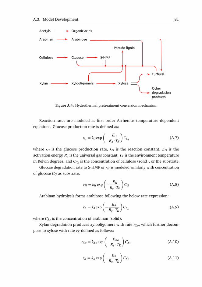
A.3. Model Development 81
Figure A.4: Hydrothermal pretreatment conversion mechanism.
Reaction rates are modeled as first order Arrhenius temperature dependent
equations. Glucose production rate is defined as:
rG = kG exp(− EG
Rg ·TK
)CCS (A.7)
where rG is the glucose production rate, kG is the reaction constant, EG is the
activation energy, Rg is the universal gas constant, TK is the environment temperature
in Kelvin degrees, and CCS is the concentration of cellulose (solid), or the substrate.
Glucose degradation rate to 5-HMF or rH is modeled similarly with concentration
of glucose CG as substrate:
rH = kH exp(− EH
Rg ·TK
)CG (A.8)
Arabinan hydrolysis forms arabinose following the below rate expression:
rA = kA exp(− EA
Rg ·TK
)CAS (A.9)
where CAS is the concentration of arabinan (solid).
Xylan degradation produces xylooligomers with rate rXo, which further decom-
pose to xylose with rate rX defined as follows:
rXo = kXo exp(− EXo
Rg ·TK
)CXS (A.10)
rX = kX exp(− EX
Rg ·TK
)CXo (A.11)
82 Paper A. Pretreatment Modeling
where CXS , and CXo are concentrations of xylan (solid), and xylooligomers (liquid).
Furfural is produced from pentoses, i.e. from both arabinose and xylose as
follows:
rF = kF exp(− EF
Rg ·TK
)(CX +CA) (A.12)
where CX and CA are concentrations of xylose (liquid) and arabinose (liquid). The
amount of furfural produced from xylose is denoted as rFX , and the one from
arabinose as rFA .
Furfural and 5-HMF bond to carbohydrates to create pseudo-lignin [53], which
is modeled in this study in the following way:
rL = kL exp(− EL
Rg ·TK
)(CXo +CX +CA +CG)(CF +CH) (A.13)
where CF is the concentration of furfural (liquid) and CH is the concentration of
5-HMF (liquid). Equation (A.13) can be split into:
rLXo = kL exp(− EL
Rg ·TK
)CXo(CF +CH)
rLX = kL exp(− EL
Rg ·TK
)CX (CF +CH)
rLA = kL exp(− EL
Rg ·TK
)CA(CF +CH)
rLG = kL exp(− EL
Rg ·TK
)CG(CF +CH)
(A.14)
which denote pseudo-lignin produced from xylooligomers, xylose, arabinose and
glucose when they bind to both furfural and 5-HMF. Then Equation (A.13) becomes:
rL = rLXo + rLX + rLA + rLG (A.15)
Equation (A.13) can also be split into:
rLF = kL exp(− EL
Rg ·TK
)(CXo +CX +CA +CG)CF
rLH = kL exp(− EL
Rg ·TK
)(CXo +CX +CA +CG)CH
(A.16)
where rLF is the production rate of pseudo-lignin with furfural participation, while
in rLH 5-HMF participates.
Acetyls are released during hemicellulose hydrolysis and lead to organic acids
formation with rate rAc:
rAc = kAc exp(− EAc
Rg ·TK
)CAcS (A.17)

A.3. Model Development 83
where CAcS is the concentration of acetyl groups in the hemicellulose (solid).
The composition vector Ck from Equation (A.6) contains all components from
the mechanistic scheme. The reaction rates from this section are put into a reaction
rates vector Rk. Ck and Rk are shown next in vector form:
Ck =
CCS
CXS
CAS
CLS
CAcS
CG
CXo
CX
CA
CAc
CF
CH
CW
CO
Rk =
−rG
−rXo
−rA
rL
−rAc
rG− rOG − (1−α)rLG
rXo− rX − (1−α)rLXo
rX − rFX − rOX − (1−α)rLX
rA− rOA − rFA − (1−α)rLA
rAc
rF −αrLF
rH −αrLH
0rOX + rOG + rOA
(A.18)
where CW is the water content, and α is a stoichiometric parameter for furfural and
5-HMF participation in pseudo-lignin formation. In order to close the mass balance,
the sum of all elements in Rk has to be 0, and the sum of all elements in vector Ck is
1000 gkg−1 at any time t:
∑Rk = 0g/(kgs) ∑Ck = 1000gkg−1 (A.19)
A.3.4 Energy Balance
The steam layer energy balance together with a temperature controller for the
thermal reactor have been formulated in Prunescu et al. [12]. The energy balance
for the biomass layer has been studied in Prunescu et al. [71] and is simplified in
this paper by a distributed parameters model on one axis, which is discretized along
the reactor, or the z axis:
dhdt
=−v∂h∂ z
+Qk⇒dhk
dt=
vδ z
(hk−1−hk)+Qk (A.20)
v is the horizontal speed, hk is the biomass enthalpy in cell k and hk−1 is the enthalpy
in the western neighbor. Qk represents the transfer of energy from steam to biomass
in cell k. As part of this coupled partial differential equation (PDE) system, the
bottom and top temperature measurements (sensors) are used to construct the
84 Paper A. Pretreatment Modeling
boundary conditions. The PDE model is then solved for obtaining the reactor
temperature gradient, which is then utilized as the temperature of the reaction in
calculating the reaction rates vector Rk.
Steam is injected through the bottom of the reactor and gets in direct contact
with the biomass. The steam injection heat transfer is lumped into the boundary
conditions of Equation (A.20). The biomass is assumed to heat till the steam
temperature near the inlet of the reactor, and used as a western boundary condition.
The heat transfer rate is computed as:
Q0 = Finh f −h0
hs0 −h0(A.21)
where Q0 is the heat transfer rate from the boundary conditions, Fin is the flow rate of
biomass, h f is the final enthalpy of heated biomass, h0 is the initial biomass enthalpy,
and hs0 is the fresh steam enthalpy. h0 is obtained by measuring the temperature of
the biomass entering the reactor T0:
h0 = cb(T0−Tr) (A.22)
where cb is the specific heat of biomass, and Tr = 0 is the reference temperature.
Biomass is assumed to have a constant specific heat of approximately cb = 3.8kJkg−1,
a value slightly lower than water (4.18 kJkg−1) since the pretreatment slurry is a mix
of condensed water and biomass.
hs0 is derived from saturated steam tables following the IAPWS-IF97 standard
[69] and from a temperature sensor Ts0 mounted in the steam supply pipe:
hs0 = f (Ts0) (A.23)
h f is computed using the temperature of the steam layer Ts measured by the top
temperature sensor, and assuming that the biomass heats till the steam temperature
near the reactor inlet:
h f = cb(Ts−Tr) (A.24)
It is natural to use the same grid in Equation (A.20) as the one from the compo-
sition balance section. The model tracks the biomass enthalpy throughout each cell
of the grid. The conductive heat from the steam to the biomass layer is neglected
due to the fact that biomass acts as an insulator. Therefore, only convective effects
remain in the biomass layer and Qk = 0,0 < k ≤ N.
The temperature profile is obtained by dividing the enthalpy from each cell with
the specific heat for biomass constant cb:
Tk =hk
cb(A.25)
where Tk is the biomass temperature from cell k, and cb is the specific heat of
pretreated biomass.
A.4. Results and Discussion 85
A.3.5 Model Summary
The thermal reactor model tracks nC = 14 species concentrations shown in vec-
tor Ck from Equation (A.18): cellulose, xylan, arabinan, lignin, acetyls, glucose,
xylooligomers, xylose, arabinose, acetic acid, furfural, 5-HMF, water, and other
components.
The total number of states nx is variable depending on the initial value of N, the
amount of cells in the reactor grid. nx can be calculated as follows:
nx = N · (nC +nh)+(ns +nm) (A.26)
where nC is the number of species, nh = 1 meaning one state for each grid cell
enthalpy, ns = 2 is the number of states from the steam layer (mass and enthalpy),
and nm = 1 is the total mass of biomass in the reactor. In this study, N is set to 10leading to 153 states in total.
The model has 2 bus inputs: one for feedstock, and another one for steam. The
feedstock input has 16 components: flow rate (1), feedstock concentrations (14),
and enthalpy (1). The steam input has 2 components: flow rate (1), and enthalpy
(1). In total there are 18 inputs.
There are 2 bus outputs: pretreated fibers and the liquid rich in C5 sugars. Each
bus has 16 components: flow rate (1), species concentrations (14), and enthalpy
(1).
Table A.3 shows the fixed model parameters. The kinetics parameters are deter-
mined in the model calibration section of this study.
A.4 Results and Discussion
This section is split into a model analysis and validation part, and the model
application as a state estimator. The model analysis and validation section contains
the sensitivity and uncertainty analysis, parameter estimation, and residual analysis.
A.4.1 Model Analysis and Validation
A.4.1.1 Model Initialization
Model parameters are calibrated with respect to the following NIR measurements:
cellulose, xylan, lignin, acetic acid and furfural. The data were obtained from a
demonstration scale thermal reactor throughout 15 h of operation. Only a subset
of 7 h is used for calibration and parameter estimation, while the entire set of
measurements is used for validation and residual analysis. The measurements of
cellulose, xylan and lignin are reported as percentage of dry matter, while acetic
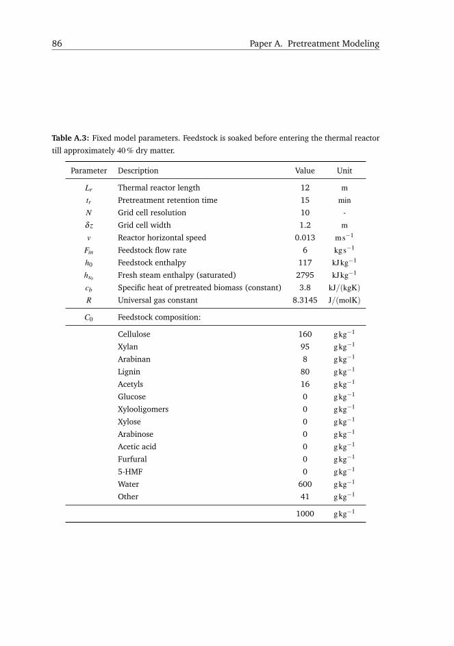
86 Paper A. Pretreatment Modeling
Table A.3: Fixed model parameters. Feedstock is soaked before entering the thermal reactor
till approximately 40 % dry matter.
Parameter Description Value Unit
Lr Thermal reactor length 12 m
tr Pretreatment retention time 15 min
N Grid cell resolution 10 -
δ z Grid cell width 1.2 m
v Reactor horizontal speed 0.013 ms−1
Fin Feedstock flow rate 6 kgs−1
h0 Feedstock enthalpy 117 kJkg−1
hs0 Fresh steam enthalpy (saturated) 2795 kJkg−1
cb Specific heat of pretreated biomass (constant) 3.8 kJ/(kgK)
R Universal gas constant 8.3145 J/(molK)
C0 Feedstock composition:
Cellulose 160 gkg−1
Xylan 95 gkg−1
Arabinan 8 gkg−1
Lignin 80 gkg−1
Acetyls 16 gkg−1
Glucose 0 gkg−1
Xylooligomers 0 gkg−1
Xylose 0 gkg−1
Arabinose 0 gkg−1
Acetic acid 0 gkg−1
Furfural 0 gkg−1
5-HMF 0 gkg−1
Water 600 gkg−1
Other 41 gkg−1
1000 gkg−1
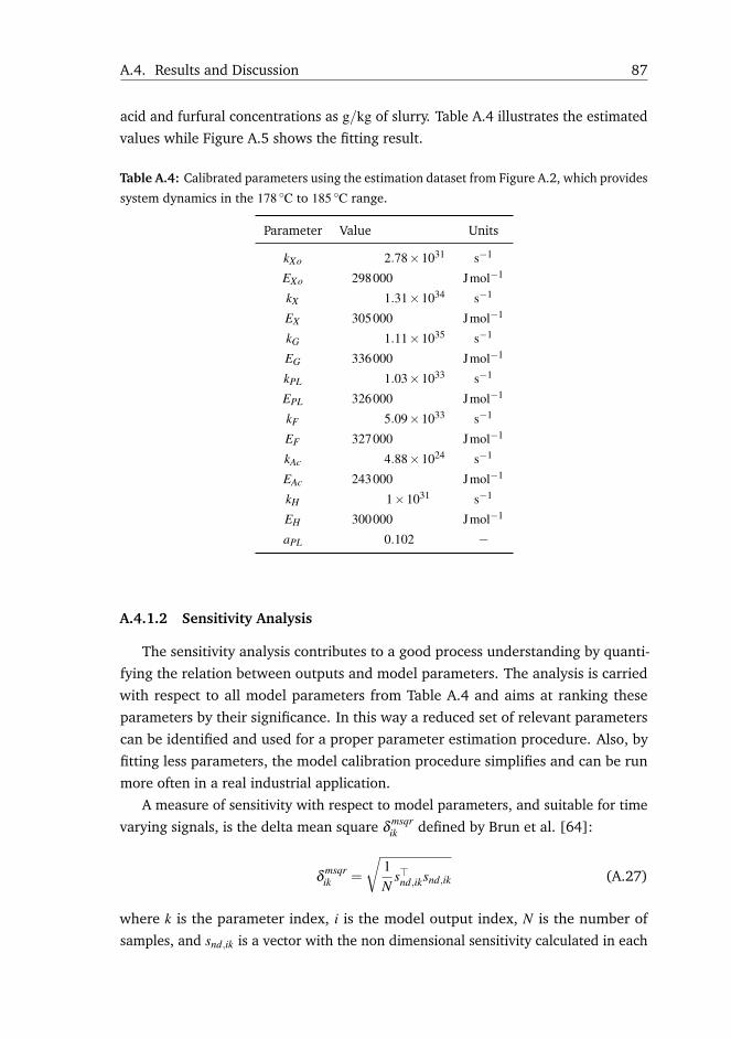
A.4. Results and Discussion 87
acid and furfural concentrations as g/kg of slurry. Table A.4 illustrates the estimated
values while Figure A.5 shows the fitting result.
Table A.4: Calibrated parameters using the estimation dataset from Figure A.2, which provides
system dynamics in the 178 ◦C to 185 ◦C range.
Parameter Value Units
kXo 2.78×1031 s−1
EXo 298000 Jmol−1
kX 1.31×1034 s−1
EX 305000 Jmol−1
kG 1.11×1035 s−1
EG 336000 Jmol−1
kPL 1.03×1033 s−1
EPL 326000 Jmol−1
kF 5.09×1033 s−1
EF 327000 Jmol−1
kAc 4.88×1024 s−1
EAc 243000 Jmol−1
kH 1×1031 s−1
EH 300000 Jmol−1
aPL 0.102 −
A.4.1.2 Sensitivity Analysis
The sensitivity analysis contributes to a good process understanding by quanti-
fying the relation between outputs and model parameters. The analysis is carried
with respect to all model parameters from Table A.4 and aims at ranking these
parameters by their significance. In this way a reduced set of relevant parameters
can be identified and used for a proper parameter estimation procedure. Also, by
fitting less parameters, the model calibration procedure simplifies and can be run
more often in a real industrial application.
A measure of sensitivity with respect to model parameters, and suitable for time
varying signals, is the delta mean square δ msqrik defined by Brun et al. [64]:
δ msqrik =
√1N
s>nd,iksnd,ik (A.27)
where k is the parameter index, i is the model output index, N is the number of
samples, and snd,ik is a vector with the non dimensional sensitivity calculated in each
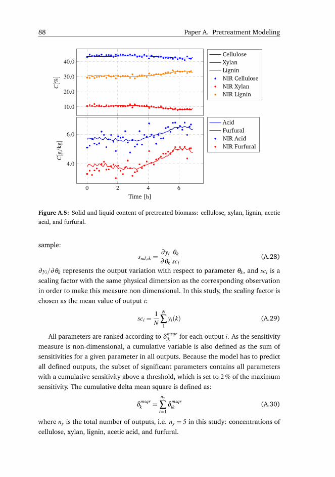
88 Paper A. Pretreatment Modeling
10.0
20.0
30.0
40.0C[%
]CelluloseXylanLigninNIR CelluloseNIR XylanNIR Lignin
0 2 4 6
4.0
6.0
Time [h]
C[g/
kg]
AcidFurfuralNIR AcidNIR Furfural
Figure A.5: Solid and liquid content of pretreated biomass: cellulose, xylan, lignin, acetic
acid, and furfural.
sample:
snd,ik =∂yi
∂θk
θk
sci(A.28)
∂yi/∂θk represents the output variation with respect to parameter θk, and sci is a
scaling factor with the same physical dimension as the corresponding observation
in order to make this measure non dimensional. In this study, the scaling factor is
chosen as the mean value of output i:
sci =1N
N
∑1
yi(k) (A.29)
All parameters are ranked according to δ msqrik for each output i. As the sensitivity
measure is non-dimensional, a cumulative variable is also defined as the sum of
sensitivities for a given parameter in all outputs. Because the model has to predict
all defined outputs, the subset of significant parameters contains all parameters
with a cumulative sensitivity above a threshold, which is set to 2 % of the maximum
sensitivity. The cumulative delta mean square is defined as:
δ msqrk =
ny
∑i=1
δ msqrik (A.30)
where ny is the total number of outputs, i.e. ny = 5 in this study: concentrations of
cellulose, xylan, lignin, acetic acid, and furfural.
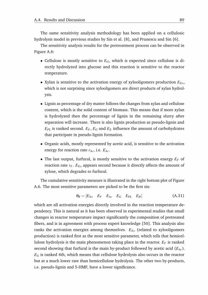
A.4. Results and Discussion 89
The same sensitivity analysis methodology has been applied on a cellulosic
hydrolysis model in previous studies by Sin et al. [8], and Prunescu and Sin [6].
The sensitivity analysis results for the pretreatment process can be observed in
Figure A.6:
• Cellulose is mostly sensitive to EG, which is expected since cellulose is di-
rectly hydrolyzed into glucose and this reaction is sensitive to the reactor
temperature.
• Xylan is sensitive to the activation energy of xylooligomers production EXo,
which is not surprising since xylooligomers are direct products of xylan hydrol-
ysis.
• Lignin as percentage of dry matter follows the changes from xylan and cellulose
content, which is the solid content of biomass. This means that if more xylan
is hydrolyzed then the percentage of lignin in the remaining slurry after
separation will increase. There is also lignin production as pseudo-lignin and
EPL is ranked second. EF , EG and EX influence the amount of carbohydrates
that participate in pseudo-lignin formation.
• Organic acids, mostly represented by acetic acid, is sensitive to the activation
energy for reaction rate rAc, i.e. EAc.
• The last output, furfural, is mostly sensitive to the activation energy EF of
reaction rate rF . EXo appears second because it directly affects the amount of
xylose, which degrades to furfural.
The cumulative sensitivity measure is illustrated in the right bottom plot of Figure
A.6. The most sensitive parameters are picked to be the first six:
θR = [EXo EF EAc EG EPL EH ] (A.31)
which are all activation energies directly involved in the reaction temperature de-
pendency. This is natural as it has been observed in experimental studies that small
changes in reactor temperature impact significantly the composition of pretreated
fibers, and is in agreement with process expert knowledge [50]. This analysis also
ranks the activation energies among themselves. EXo (related to xylooligomers
production) is ranked first as the most sensitive parameter, which tells that hemicel-
lulose hydrolysis is the main phenomenon taking place in the reactor. EF is ranked
second showing that furfural is the main by-product followed by acetic acid (EAc).
EG is ranked 4th, which means that cellulose hydrolysis also occurs in the reactor
but at a much lower rate than hemicellulose hydrolysis. The other two by-products,
i.e. pseudo-lignin and 5-HMF, have a lower significance.
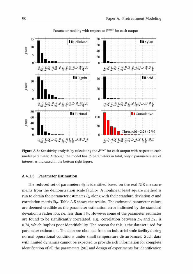
90 Paper A. Pretreatment Modeling
EG
EX
oE
PL
EF
EA
cE
H k G k Xo
k PL
EX
k Ac
k F k H a PL k X
0
5
10
15
δmsq
r
Cellulose
EX
oE
GE
PL
EF
k Xo
EA
cE
H k G k PL
k Ac
EX k F k H k X a PL
0
20
40
60
80Xylan
EG
EX
oE
PL
EF
EH
EA
ck G k X
ok P
LE
X k F k H k Ac
a PL k X
0
5
10
δmsq
r
Lignin
EA
cE
GE
Xo
k Ac
EP
LE
FE
Hk X
ok G k P
LE
X k F k X k H a PL
0
20
40 Acid
EF
EX
oE
PL
EG k F EX
EH
k Xo
EA
ck P
La P
L k G k H k X k Ac
0
20
40
60
80
δmsq
r
Furfural
EX
oE
FE
Ac
EG
EP
LE
Hk X
oE
X k F k Ac
k G k PL
a PL
k H k X
0
50
100
Threshold=2.28 (2 %)
Cumulative
Parameter ranking with respect to δ msqr for each output
Figure A.6: Sensitivity analysis by calculating the δ msqr for each output with respect to each
model parameter. Although the model has 15 parameters in total, only 6 parameters are of
interest as indicated in the bottom right figure.
A.4.1.3 Parameter Estimation
The reduced set of parameters θR is identified based on the real NIR measure-
ments from the demonstration scale facility. A nonlinear least square method is
run to obtain the parameter estimates θR along with their standard deviation σ and
correlation matrix Rθ . Table A.5 shows the results. The estimated parameter values
are deemed credible as the parameter estimation error indicated by the standard
deviation is rather low, i.e. less than 1 %. However some of the parameter estimates
are found to be significantly correlated, e.g. correlation between EG and EXo is
0.74, which implies poor identifiability. The reason for this is the dataset used for
parameter estimation. The data are obtained from an industrial scale facility during
normal operational conditions under small temperature disturbances. Such data
with limited dynamics cannot be expected to provide rich information for complete
identification of all the parameters [98] and design of experiments for identification

A.4. Results and Discussion 91
should be pursued on lower scale facilities. Other measurements should also be
included in the parameter estimation analysis, such as xylooligomers, xylose and
glucose content of the liquid part, which are missing in this study.
Table A.5: Parameter estimation results. The estimates of the most important parameters
with their standard deviations are shown in Table A.6(a). The correlation matrix is displayed
in Table A.6(b). The results are valid in the 178 ◦C to 185 ◦C range.
(a) Parameter estimates in Jmol−1 with standard deviation σ and 95 % confidence interval.
Parameter Value [Jmol−1] Standard deviation σ Lower bound Upper bound
EXo 298010 98 297918 298102
EF 327255 285 326989 327520
EAc 242693 174 242531 242855
EG 335616 249 335383 335848
EPL 325632 1573 324165 327099
EH 299999 2639 297537 302461
(b) Correlation matrix Rθ .
Parameter EXo EF EAc EG EPL EH
EXo 1
EF −0.51 1
EAc 0.17 −0.12 1
EG 0.74 −0.54 0.26 1
EPL −0.51 0.74 −0.15 −0.63 1
EH 0.14 −0.61 0.01 0.16 −0.85 1
A.4.1.4 Uncertainty Analysis
In order to assess the uncertainty of the model, a large number of Monte Carlo
simulations are run in 3 different scenarios that cover most sources of uncertainty:
model parameters, feed parameters, and combined.
1. Model parameters uncertainty: the standard deviation and the correlation
matrix for model parameters were obtained in the previous step. A number of
200 samples are generated using Latin hypercube sampling with correlation
control. Figure A.7(a) shows the biomass composition predictions with the
5th-95th percentile interval considering only model parameters uncertainty.
The model parameters uncertainty cannot explain the entire output variations,
especially in the solid content of the mixture. This is expected since there
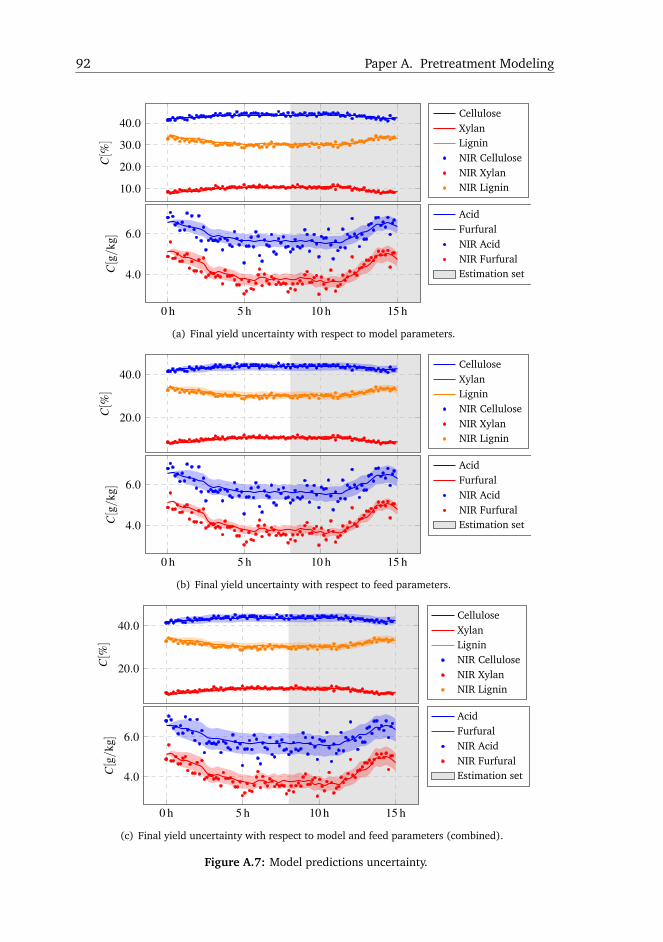
92 Paper A. Pretreatment Modeling
10.0
20.0
30.0
40.0
C[%
]CelluloseXylanLigninNIR CelluloseNIR XylanNIR Lignin
0 h 5 h 10 h 15 h
4.0
6.0
C[g/k
g]
AcidFurfuralNIR AcidNIR FurfuralEstimation set
(a) Final yield uncertainty with respect to model parameters.
20.0
40.0
C[%
]
CelluloseXylanLigninNIR CelluloseNIR XylanNIR Lignin
0 h 5 h 10 h 15 h
4.0
6.0
C[g/k
g]
AcidFurfuralNIR AcidNIR FurfuralEstimation set
(b) Final yield uncertainty with respect to feed parameters.
20.0
40.0
C[%
]
CelluloseXylanLigninNIR CelluloseNIR XylanNIR Lignin
0 h 5 h 10 h 15 h
4.0
6.0
C[g/k
g]
AcidFurfuralNIR AcidNIR FurfuralEstimation set
(c) Final yield uncertainty with respect to model and feed parameters (combined).
Figure A.7: Model predictions uncertainty.
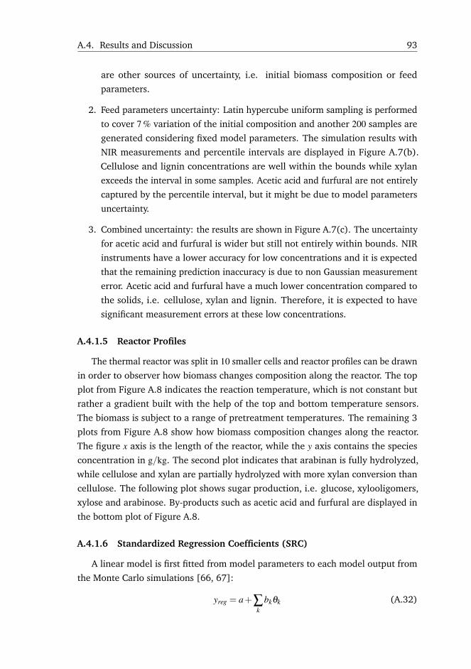
A.4. Results and Discussion 93
are other sources of uncertainty, i.e. initial biomass composition or feed
parameters.
2. Feed parameters uncertainty: Latin hypercube uniform sampling is performed
to cover 7 % variation of the initial composition and another 200 samples are
generated considering fixed model parameters. The simulation results with
NIR measurements and percentile intervals are displayed in Figure A.7(b).
Cellulose and lignin concentrations are well within the bounds while xylan
exceeds the interval in some samples. Acetic acid and furfural are not entirely
captured by the percentile interval, but it might be due to model parameters
uncertainty.
3. Combined uncertainty: the results are shown in Figure A.7(c). The uncertainty
for acetic acid and furfural is wider but still not entirely within bounds. NIR
instruments have a lower accuracy for low concentrations and it is expected
that the remaining prediction inaccuracy is due to non Gaussian measurement
error. Acetic acid and furfural have a much lower concentration compared to
the solids, i.e. cellulose, xylan and lignin. Therefore, it is expected to have
significant measurement errors at these low concentrations.
A.4.1.5 Reactor Profiles
The thermal reactor was split in 10 smaller cells and reactor profiles can be drawn
in order to observer how biomass changes composition along the reactor. The top
plot from Figure A.8 indicates the reaction temperature, which is not constant but
rather a gradient built with the help of the top and bottom temperature sensors.
The biomass is subject to a range of pretreatment temperatures. The remaining 3
plots from Figure A.8 show how biomass composition changes along the reactor.
The figure x axis is the length of the reactor, while the y axis contains the species
concentration in g/kg. The second plot indicates that arabinan is fully hydrolyzed,
while cellulose and xylan are partially hydrolyzed with more xylan conversion than
cellulose. The following plot shows sugar production, i.e. glucose, xylooligomers,
xylose and arabinose. By-products such as acetic acid and furfural are displayed in
the bottom plot of Figure A.8.
A.4.1.6 Standardized Regression Coefficients (SRC)
A linear model is first fitted from model parameters to each model output from
the Monte Carlo simulations [66, 67]:
yreg = a+∑k
bkθk (A.32)
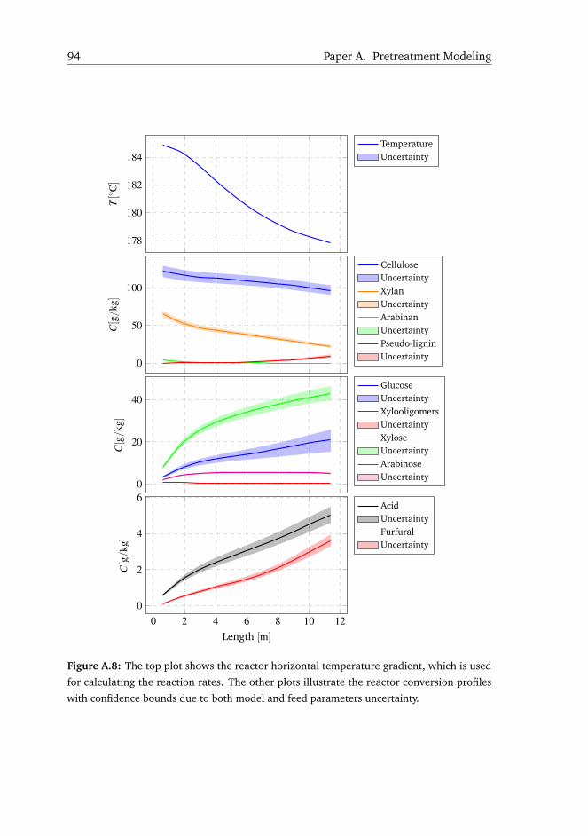
94 Paper A. Pretreatment Modeling
178
180
182
184
T[◦
C]
TemperatureUncertainty
0
50
100
C[g/
kg]
CelluloseUncertaintyXylanUncertaintyArabinanUncertaintyPseudo-ligninUncertainty
0
20
40
C[g/k
g]
GlucoseUncertaintyXylooligomersUncertaintyXyloseUncertaintyArabinoseUncertainty
0 2 4 6 8 10 120
2
4
6
Length [m]
C[g/k
g]
AcidUncertaintyFurfuralUncertainty
Figure A.8: The top plot shows the reactor horizontal temperature gradient, which is used
for calculating the reaction rates. The other plots illustrate the reactor conversion profiles
with confidence bounds due to both model and feed parameters uncertainty.
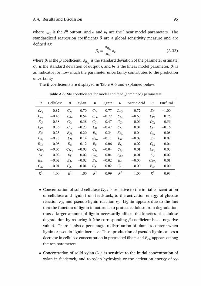
A.4. Results and Discussion 95
where yreg is the ith output, and a and bk are the linear model parameters. The
standardized regression coefficients β are a global sensitivity measure and are
defined as:
βk =σθRk
σyi
bk (A.33)
where βk is the β coefficient, σθRkis the standard deviation of the parameter estimate,
σyi is the standard deviation of output i, and bk is the linear model parameter. βk is
an indicator for how much the parameter uncertainty contributes to the prediction
uncertainty.
The β coefficients are displayed in Table A.6 and explained below:
Table A.6: SRC coefficients for model and feed (combined) parameters.
θ Cellulose θ Xylan θ Lignin θ Acetic Acid θ Furfural
CCS 0.82 CXS 0.70 CLS 0.77 CACS 0.72 EF −1.00
CLS −0.43 EXo 0.54 EPL −0.72 EAc −0.60 EPL 0.75
EG 0.38 CCS −0.38 CCS −0.47 CCS 0.06 CXS 0.56
EPL 0.36 CLS −0.23 EH −0.47 CLS 0.04 EXo −0.16
EH 0.23 EPL 0.20 EG −0.24 EPL −0.04 CAS 0.08
CXS −0.23 EH 0.14 EXo −0.11 EH −0.02 EH 0.07
EXo −0.08 EG −0.12 EF −0.06 EG 0.02 CLS 0.04
CACS −0.05 CACS −0.03 CXS −0.04 CXS 0.01 CCS 0.03
EF 0.02 EF 0.02 CACS −0.04 EXo 0.01 EG 0.02
EAc −0.02 EAc −0.02 EAc −0.02 EF −0.00 CACS 0.01
CAS −0.01 CAS −0.01 CAS 0.02 CAS −0.00 EAc 0.00
R2 1.00 R2 1.00 R2 0.99 R2 1.00 R2 0.93
• Concentration of solid cellulose CCS : is sensitive to the initial concentration
of cellulose and lignin from feedstock, to the activation energy of glucose
reaction rG, and pseudo-lignin reaction rL. Lignin appears due to the fact
that the function of lignin in nature is to protect cellulose from degradation,
thus a larger amount of lignin necessarily affects the kinetics of cellulose
degradation by reducing it (the corresponding β coefficient has a negative
value). There is also a percentage redistribution of biomass content when
lignin or pseudo-lignin increase. Thus, production of pseudo-lignin causes a
decrease in cellulose concentration in pretreated fibers and EPL appears among
the top parameters.
• Concentration of solid xylan CXS : is sensitive to the initial concentration of
xylan in feedstock, and to xylan hydrolysis or the activation energy of xy-
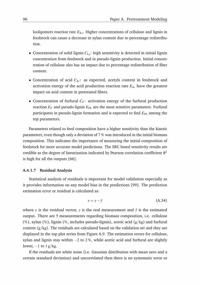
96 Paper A. Pretreatment Modeling
looligomers reaction rate EXo. Higher concentrations of cellulose and lignin in
feedstock can cause a decrease in xylan content due to percentage redistribu-
tion.
• Concentration of solid lignin CLS : high sensitivity is detected in initial lignin
concentration from feedstock and in pseudo-lignin production. Initial concen-
tration of cellulose also has an impact due to percentage redistribution of fiber
content.
• Concentration of acid CAc: as expected, acetyls content in feedstock and
activation energy of the acid production reaction rate EAc have the greatest
impact on acid content in pretreated fibers.
• Concentration of furfural CF : activation energy of the furfural production
reaction EF and pseudo-lignin EPL are the most sensitive parameters. Furfural
participates in pseudo-lignin formation and is expected to find EPL among the
top parameters.
Parameters related to feed composition have a higher sensitivity than the kinetic
parameters, even though only a deviation of 7 % was introduced in the initial biomass
composition. This indicates the importance of measuring the initial composition of
feedstock for more accurate model predictions. The SRC based sensitivity results are
credible as the degree of linearization indicated by Pearson correlation coefficient R2
is high for all the outputs [66].
A.4.1.7 Residual Analysis
Statistical analysis of residuals is important for model validation especially as
it provides information on any model bias in the predictions [99]. The prediction
estimation error or residual is calculated as:
e = y− y (A.34)
where e is the residual vector, y is the real measurement and y is the estimated
output. There are 5 measurements regarding biomass composition, i.e. cellulose
(%), xylan (%), lignin (%, includes pseudo-lignin), acetic acid (g/kg) and furfural
content (g/kg). The residuals are calculated based on the validation set and they are
displayed in the top plot series from Figure A.9. The estimation errors for cellulose,
xylan and lignin stay within −2 to 2 %, while acetic acid and furfural are slightly
lower, −1 to 1 g/kg.
If the residuals are white noise (i.e. Gaussian distribution with mean zero and a
certain standard deviation) and uncorrelated then there is no systematic error or
A.4. Results and Discussion 97
bias in the model. To check the hypothesis of residual Gaussian distribution, a 5 %t-test is performed. The test is passed and the Gaussian probability plots from Figure
A.9 (the middle series) show how close the residuals are to a Normal distribution.
The autocorrelation determines if there still is any information in the residuals that
is not captured by the model. The bottom series of plots from Figure A.9 display
the autocorrelation function at 50 lags with the 95 % confidence interval. There are
spikes in almost all plots except acetic acid production that exceed the confidence
interval but they are not significant. The feedstock composition and the assumption
that it remains constant might be a good source for these results. In reality feedstock
has composition variations.
−2.0
0.0
2.0
Res
idua
ls[%
]
Cellulose Xylan Lignin Acid
Res
idua
ls[g/k
g]
Furfural
0.05
0.5
0.95
Prob
abili
ty
0
0.5
1
Aut
ocor
rela
tion
Figure A.9: Residual analysis for the validation set. The top plot series show the residuals;
the middle series compare in a Gaussian probability plot the distribution of residuals to a
Normal distribution; the bottom series display the autocorrelation function and the 95 %
confidence interval.
A.4.2 Model Application: State Estimator
The utility of the model for industrial application is highlighted through the
development of a state estimator using a Kalman filter. The state estimator is useful
for performance monitoring by estimating in real-time the entire biomass compo-
sition, i.e. both sugars and inhibitors production. The estimator infers all species
concentrations from pretreated fibers using a reduced number of measurements
provided by the NIR instrument.
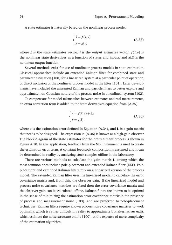
98 Paper A. Pretreatment Modeling
A state estimator is naturally based on the nonlinear process model:
{ˆx = f (x,u)
y = g(x)(A.35)
where x is the state estimates vector, y is the output estimates vector, f (x,u) is
the nonlinear state derivatives as a function of states and inputs, and g(x) is the
nonlinear output function.
Several methods exist for use of nonlinear process models in state estimation.
Classical approaches include an extended Kalman filter for combined state and
parameter estimation [100] for a linearized system at a particular point of operation,
or direct inclusion of the nonlinear process model in the filter [101]. Later develop-
ments have included the unscented Kalman and particle filters to better explore and
approximate non-Gaussian nature of the process noise in a nonlinear system [102].
To compensate for model-mismatches between estimates and real measurements,
an extra correction term is added to the state derivatives equation from (A.35):
{ˆx = f (x,u)+Le
y = g(x)(A.36)
where e is the estimation error defined in Equation (A.34), and L is a gain matrix
that needs to be designed. The expression in (A.36) is known as a high-gain observer.
The block diagram of the state estimator for the pretreatment process is shown in
Figure A.10. In this application, feedback from the NIR instrument is used to create
the estimation error term. A constant feedstock composition is assumed and it can
be determined in reality by analyzing stock samples offline in the laboratory.
There are various methods to calculate the gain matrix L among which the
most common ones include pole-placement and extended Kalman filter (EKF). Pole-
placement and extended Kalman filters rely on a linearized version of the process
model. The extended Kalman filter uses the linearized model to calculate the error
covariance matrix and, from this, the observer gain. If the linearized model and
process noise covariance matrices are fixed then the error covariance matrix and
the observer gain can be calculated offline. Kalman filters are known to be optimal
in the sense of minimizing the estimation error covariance matrix in the presence
of process and measurement noise [103], and are preferred to pole-placement
techniques. Kalman filters require known process noise covariance matrices to work
optimally, which is rather difficult in reality to approximate but alternatives exist,
which estimate the noise structure online [100], at the expense of more complexity
of the estimation algorithm.
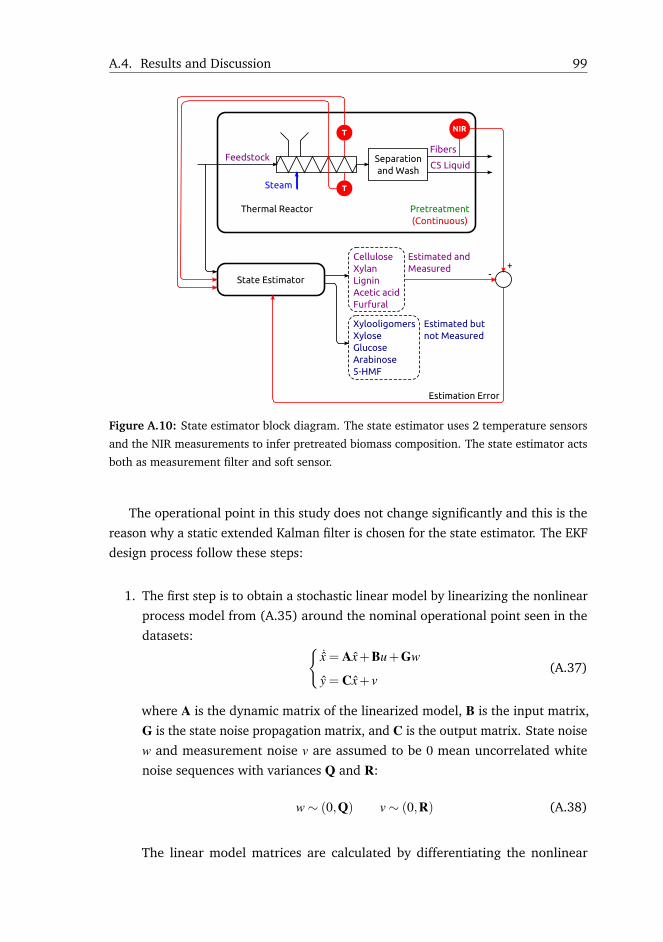
A.4. Results and Discussion 99
Figure A.10: State estimator block diagram. The state estimator uses 2 temperature sensors
and the NIR measurements to infer pretreated biomass composition. The state estimator acts
both as measurement filter and soft sensor.
The operational point in this study does not change significantly and this is the
reason why a static extended Kalman filter is chosen for the state estimator. The EKF
design process follow these steps:
1. The first step is to obtain a stochastic linear model by linearizing the nonlinear
process model from (A.35) around the nominal operational point seen in the
datasets: {˙x = Ax+Bu+Gw
y = Cx+ v(A.37)
where A is the dynamic matrix of the linearized model, B is the input matrix,
G is the state noise propagation matrix, and C is the output matrix. State noise
w and measurement noise v are assumed to be 0 mean uncorrelated white
noise sequences with variances Q and R:
w∼ (0,Q) v∼ (0,R) (A.38)
The linear model matrices are calculated by differentiating the nonlinear
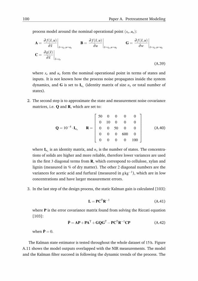
100 Paper A. Pretreatment Modeling
process model around the nominal operational point (xe,ue):
A =∂ f (x,u)
∂ x
∣∣∣∣x=xe,u=ue
B =∂ f (x,u)
∂u
∣∣∣∣x=xe,u=ue
G =∂ f (x,u)
∂w
∣∣∣∣x=xe,u=ue
C =∂g(x)
∂ x
∣∣∣∣x=xe
(A.39)
where xe and ue form the nominal operational point in terms of states and
inputs. It is not known how the process noise propagates inside the system
dynamics, and G is set to Inx (identity matrix of size nx or total number of
states).
2. The second step is to approximate the state and measurement noise covariance
matrices, i.e. Q and R, which are set to:
Q = 10−4 · Inx R =
50 0 0 0 00 10 0 0 00 0 50 0 00 0 0 600 00 0 0 0 100
(A.40)
where Inx is an identity matrix, and nx is the number of states. The concentra-
tions of solids are higher and more reliable, therefore lower variances are used
in the first 3 diagonal terms from R, which correspond to cellulose, xylan and
lignin (measured in % of dry matter). The other 2 diagonal numbers are the
variances for acetic acid and furfural (measured in gkg−1), which are in low
concentrations and have larger measurement errors.
3. In the last step of the design process, the static Kalman gain is calculated [103]:
L = PCTR−1 (A.41)
where P is the error covariance matrix found from solving the Riccati equation
[103]:
P = AP+PAT +GQGT−PCTR−1CP (A.42)
when P = 0.
The Kalman state estimator is tested throughout the whole dataset of 15 h. Figure
A.11 shows the model outputs overlapped with the NIR measurements. The model
and the Kalman filter succeed in following the dynamic trends of the process. The
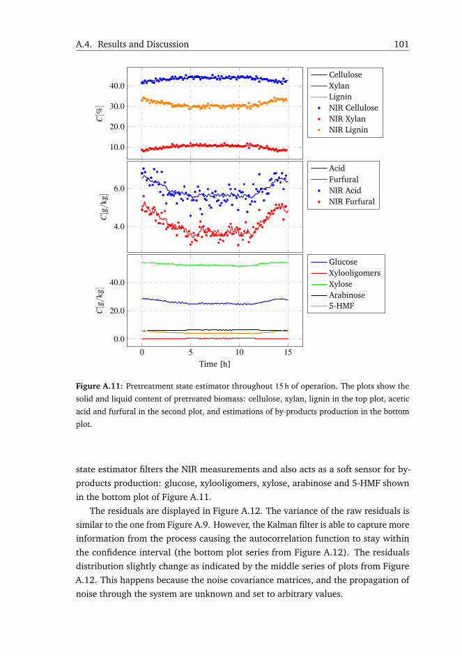
A.4. Results and Discussion 101
10.0
20.0
30.0
40.0C[%
]
CelluloseXylanLigninNIR CelluloseNIR XylanNIR Lignin
4.0
6.0
C[g/k
g]
AcidFurfuralNIR AcidNIR Furfural
0 5 10 15
0.0
20.0
40.0
Time [h]
C[g/
kg]
GlucoseXylooligomersXyloseArabinose5-HMF
Figure A.11: Pretreatment state estimator throughout 15 h of operation. The plots show the
solid and liquid content of pretreated biomass: cellulose, xylan, lignin in the top plot, acetic
acid and furfural in the second plot, and estimations of by-products production in the bottom
plot.
state estimator filters the NIR measurements and also acts as a soft sensor for by-
products production: glucose, xylooligomers, xylose, arabinose and 5-HMF shown
in the bottom plot of Figure A.11.
The residuals are displayed in Figure A.12. The variance of the raw residuals is
similar to the one from Figure A.9. However, the Kalman filter is able to capture more
information from the process causing the autocorrelation function to stay within
the confidence interval (the bottom plot series from Figure A.12). The residuals
distribution slightly change as indicated by the middle series of plots from Figure
A.12. This happens because the noise covariance matrices, and the propagation of
noise through the system are unknown and set to arbitrary values.
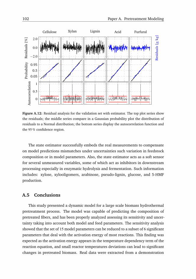
102 Paper A. Pretreatment Modeling
−2.0
0.0
2.0
Res
idua
ls[%
]
Cellulose Xylan Lignin Acid
Res
idua
ls[g/k
g]
Furfural
0.05
0.5
0.95
Prob
abili
ty
0
0.5
1
Aut
ocor
rela
tion
Figure A.12: Residual analysis for the validation set with estimator. The top plot series show
the residuals; the middle series compare in a Gaussian probability plot the distribution of
residuals to a Normal distribution; the bottom series display the autocorrelation function and
the 95 % confidence region.
The state estimator successfully embeds the real measurements to compensate
on model predictions mismatches under uncertainties such variation in feedstock
composition or in model parameters. Also, the state estimator acts as a soft sensor
for several unmeasured variables, some of which act as inhibitors in downstream
processing especially in enzymatic hydrolysis and fermentation. Such information
includes: xylose, xylooligomers, arabinose, pseudo-lignin, glucose, and 5-HMF
production.
A.5 Conclusions
This study presented a dynamic model for a large scale biomass hydrothermal
pretreatment process. The model was capable of predicting the composition of
pretreated fibers, and has been properly analyzed assessing its sensitivity and uncer-
tainty taking into account both model and feed parameters. The sensitivity analysis
showed that the set of 15 model parameters can be reduced to a subset of 6 significant
parameters that deal with the activation energy of most reactions. This finding was
expected as the activation energy appears in the temperature dependency term of the
reaction equation, and small reactor temperatures deviations can lead to significant
changes in pretreated biomass. Real data were extracted from a demonstration
A.5. Conclusions 103
scale biorefinery and used for parameter estimation and model validation. The data
exhibit limited system dynamics and provide a range of validity for the parameter
estimates between 178 ◦C to 185 ◦C. In order to extend the validity range of the
parameter estimates to different temperature ranges, additional experimental data
should be collected either by experimenting at lower scale facilities or changing the
operational points of the biorefinery, which is not easily accessible.
The uncertainty analysis was conducted with Latin hypercube sampling of both
model and feed parameters, and Monte Carlo simulations. The 5th-95th percentile
includes most of the real data variations, except the very low concentrations of
acetic acid and furfural, which is expected as the NIR instrument is affected by
high measurement errors at low concentrations. The global sensitivity analysis
showed that feedstock composition parameters have a higher significance than model
parameters, suggesting that feedstock composition should be measured upstream
for more accurate predictions.
In the last section of the study, a Kalman state estimator was designed as an
application of the process model. The estimator was then tested on the whole
dataset, i.e. throughout 15 h of operation. The model predictions were found to
follow the dynamic trends of the process, making it valuable for control design,
diagnosis, real-time optimization, and inferential sensors development at full scale
applications. The state estimator acts both as a measurement filter and soft sensor
for estimating unmeasured variables, i.e. C5 sugars production and inhibitors, which
are important in downstream processes.

Paper B
Dynamic Modeling andValidation of a LignocellulosicEnzymatic Hydrolysis Process - ADemonstration Scale Study
Remus Mihail Prunescu1, Gürkan Sin*2
1Department of Electrical Engineering, Automation and Control Group, Technical
University of Denmark, Elektrovej Building 326, 2800, Kgs. Lyngby, Denmark
2CAPEC-PROCESS, Department of Chemical and Biochemical Engineering, Technical
University of Denmark, Søltofts Plads Buildings 227 and 229, 2800, Kgs. Lyngby,
Denmark
Abstract:
The enzymatic hydrolysis process is one of the key steps in second generation biofuel
production. After being thermally pretreated, the lignocellulosic material is liquefied
by enzymes prior to fermentation. The scope of this paper is to evaluate a dynamic
model of the hydrolysis process on a demonstration scale reactor. The following
novel features are included: the application of the Convection-Diffusion-Reaction
equation to a hydrolysis reactor to assess transport and mixing effects; the extension
of a competitive kinetic model with enzymatic pH dependency and hemicellulose
hydrolysis; a comprehensive pH model; and viscosity estimations during the course
of reaction. The model is evaluated against real data extracted from a demonstration
scale biorefinery throughout several days of operation. All measurements are within
predictions uncertainty and, therefore, the model constitutes a valuable tool to
support process optimization, performance monitoring, diagnosis and process control
at full-scale studies.
*Principal corresponding author. Tel.: +45 45252806; E-mail: [email protected]
106 Paper B. Enzymatic Hydrolysis Modeling
B.1 Introduction
Bioethanol is thought to become a viable alternative to fossil fuels [1] and many
countries with agricultural resources show an increasing interest in the second
generation biofuel production technology, especially in USA, Brazil, Denmark and
Italy. The latest developments that approach biorefineries to a commercial reality
are presented by Larsen et al. [3].
In biorefinery concepts that employ a biochemical conversion route, the ligno-
cellulosic material originating from agricultural wastes is typically transformed into
bioethanol following 4 major steps, i.e. pretreatment, enzymatic hydrolysis, fermen-
tation and separation [4]. The pretreated lignocellulosic material has a high content
of cellulose, hemicellulose and lignin. The purpose of the enzymatic hydrolysis
process is to break down the long polymeric chains of cellulose and xylan into its
constituent sugar units, mostly glucose and xylose.
The underlying mechanism of the enzymatic hydrolysis process is a complex one,
which has been the target of many modeling studies. Kadam et al. [60] formulate a
mechanistic conversion model while Zhang and Lynd [104] explain in detail how the
cellulosic depolymerization occurs under the effect of enzymes. The Kadam model
has been validated in laboratory scale experiments both by Kadam et al. [60] and
Hodge et al. [105]. Sin et al. [8] have performed an identifiability and uncertainty
analysis of the Kadam model and Morales-Rodriguez et al. [96] have integrated
it into a dynamic modeling framework for assessing biorefinery configurations.
The depolymerization model has been extended and validated in laboratory scale
experiments by Hosseini and Shah [106, 107]. So far, none of these models have
been evaluated at a realistic demonstration scale.
In order to formulate a model for large scale biorefineries, several extensions
need to be made to the previous models. pH calculations were not performed
before although it is well known that enzymes are sensitive to pH following a
Gaussian curve. At laboratory scale, perfect pH control can be easily achieved
and assumed but at larger scales such control becomes challenging. When the
process runs in a continuous manner, the inflow composition varies due to different
pretreatment conditions or biomass composition and the concentration of acetic
acid has disturbances that affect the pH level [12]. Also, previous models do not
include xylan hydrolysis, which contributes to acetic acid formation inside the
reactor leading to a pH profile along the container that affects the enzymatic activity.
Another missing feature is viscosity calculations, which are important for estimating
diffusion coefficients and for assessing transportation and mixing effects.
With these in background, a dynamic lignocellulosic hydrolysis model adequate
B.2. Materials and Methods 107
for demonstration and large scale processes is formulated with the following fea-
tures: the reactor is modeled as plug flow using the Convection-Diffusion-Reaction
(CDR) equation in one dimension in order to capture properly transport and mixing
effects along the length of the tank, i.e. the x axis; the reaction kinetics comprises
competitive cellulose and xylan hydrolysis with temperature and pH dependency
plus furfural inhibition; pH dynamics account for most of the relevant buffers that
come from the pretreatment process, i.e. acetic, succinic and lactic acids plus a
bicarbonate formation system with CO2 stripping effects. Chemical kinetics, and pH
and viscosity calculations are tracked in each cell of the 1-D CDR model.
The model is then analyzed in order to assess its sensitivity to kinetic and feed
parameters, and to quantify its predictions uncertainty.
This paper is structured as follows: section B.2 describes a typical demonstration
scale biorefinery and how measurements were recorded for comparing against
model predictions; section B.3 formulates the mathematical model and includes its
sensitivity and uncertainty analysis; and section B.4 illustrates and discusses the
model validation results.
B.2 Materials and Methods
A demonstration scale biorefinery is capable of transforming approximately
4 th−1 of biomass into three products, i.e. 576 kgh−1 2G bioethanol, 1484 kgh−1 C5
molasses and 1740 kgh−1 lignin pallets [3]. The biomass can be any lignocellulosic
material, preferably agricultural wastes, e.g. straw, bagasses or corn stover, or
forest wastes, e.g. saw dust, pulp waste or thinned wood [108]. There are various
biomass pretreatment methods, e.g. autohydrolysis, steam explosion, acid hydrolysis
etc., among which steam explosion is seen as a cheap and environmentally friendly
pretreatment [44]. In this investigation, wheat straw was pretreated with steam in a
large pressurized thermal reactor described in [71].
Figure B.1 illustrates the biomass conversion route with emphasis on the enzy-
matic hydrolysis process. The inflow of pretreated fibers is denoted as FFF and has
an initial chemical composition C0, which is measured with online NIR equipment
that performs a measurement every 5 min. A strong base, i.e. NaOH, is pumped into
the tank near the inlet for pH adjustments. The base inflow FB and its concentration
CB are considered known. A certain amount of enzymes proportional to cellulose
content from the pretreated fibers is added by a pump from a storage tank. The
flow of enzymes FE and its concentration CE are considered known. Water is also
added with a known flow rate FW . The reactor is mass controlled using a mass
measurement MFM and by manipulating the outflow of fiber mash FFM. The outflow
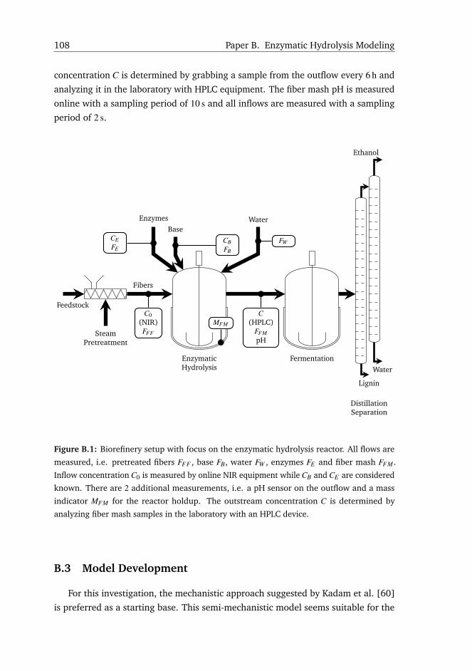
108 Paper B. Enzymatic Hydrolysis Modeling
concentration C is determined by grabbing a sample from the outflow every 6 h and
analyzing it in the laboratory with HPLC equipment. The fiber mash pH is measured
online with a sampling period of 10 s and all inflows are measured with a sampling
period of 2 s.
Feedstock
SteamPretreatment
Fibers
EnzymaticHydrolysis
EnzymesBase
Fermentation
Water
Ethanol
Lignin
Water
DistillationSeparation
C0(NIR)FFF
CEFE
CBFB
FW
C(HPLC)
FFMpH
MFM
Figure B.1: Biorefinery setup with focus on the enzymatic hydrolysis reactor. All flows are
measured, i.e. pretreated fibers FFF , base FB, water FW , enzymes FE and fiber mash FFM .
Inflow concentration C0 is measured by online NIR equipment while CB and CE are considered
known. There are 2 additional measurements, i.e. a pH sensor on the outflow and a mass
indicator MFM for the reactor holdup. The outstream concentration C is determined by
analyzing fiber mash samples in the laboratory with an HPLC device.
B.3 Model Development
For this investigation, the mechanistic approach suggested by Kadam et al. [60]
is preferred as a starting base. This semi-mechanistic model seems suitable for the
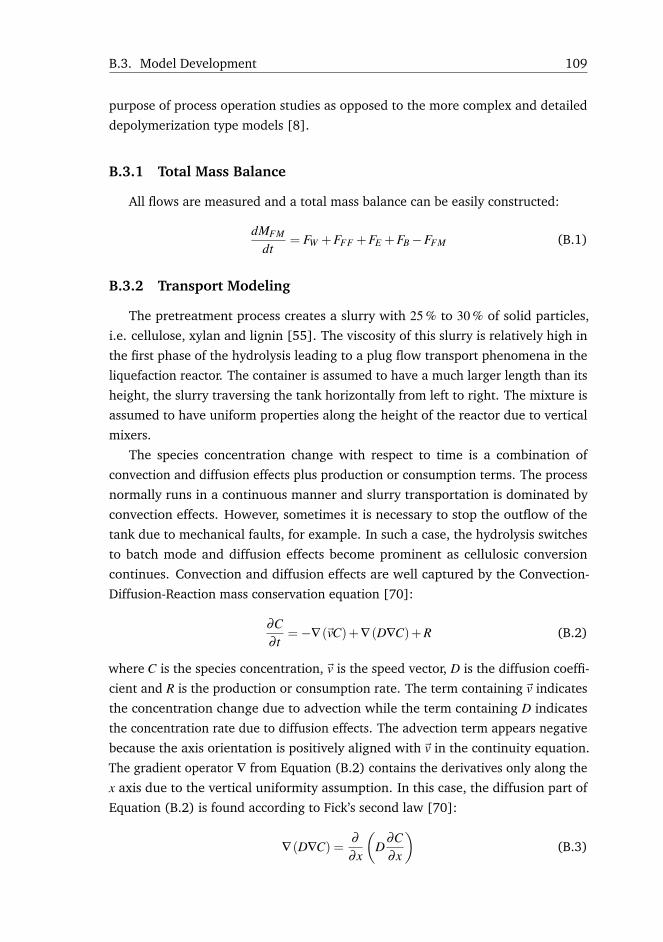
B.3. Model Development 109
purpose of process operation studies as opposed to the more complex and detailed
depolymerization type models [8].
B.3.1 Total Mass Balance
All flows are measured and a total mass balance can be easily constructed:
dMFM
dt= FW +FFF +FE +FB−FFM (B.1)
B.3.2 Transport Modeling
The pretreatment process creates a slurry with 25 % to 30 % of solid particles,
i.e. cellulose, xylan and lignin [55]. The viscosity of this slurry is relatively high in
the first phase of the hydrolysis leading to a plug flow transport phenomena in the
liquefaction reactor. The container is assumed to have a much larger length than its
height, the slurry traversing the tank horizontally from left to right. The mixture is
assumed to have uniform properties along the height of the reactor due to vertical
mixers.
The species concentration change with respect to time is a combination of
convection and diffusion effects plus production or consumption terms. The process
normally runs in a continuous manner and slurry transportation is dominated by
convection effects. However, sometimes it is necessary to stop the outflow of the
tank due to mechanical faults, for example. In such a case, the hydrolysis switches
to batch mode and diffusion effects become prominent as cellulosic conversion
continues. Convection and diffusion effects are well captured by the Convection-
Diffusion-Reaction mass conservation equation [70]:
∂C∂ t
=−∇(~vC)+∇(D∇C)+R (B.2)
where C is the species concentration,~v is the speed vector, D is the diffusion coeffi-
cient and R is the production or consumption rate. The term containing~v indicates
the concentration change due to advection while the term containing D indicates
the concentration rate due to diffusion effects. The advection term appears negative
because the axis orientation is positively aligned with~v in the continuity equation.
The gradient operator ∇ from Equation (B.2) contains the derivatives only along the
x axis due to the vertical uniformity assumption. In this case, the diffusion part of
Equation (B.2) is found according to Fick’s second law [70]:
∇(D∇C) =∂∂x
(D
∂C∂x
)(B.3)
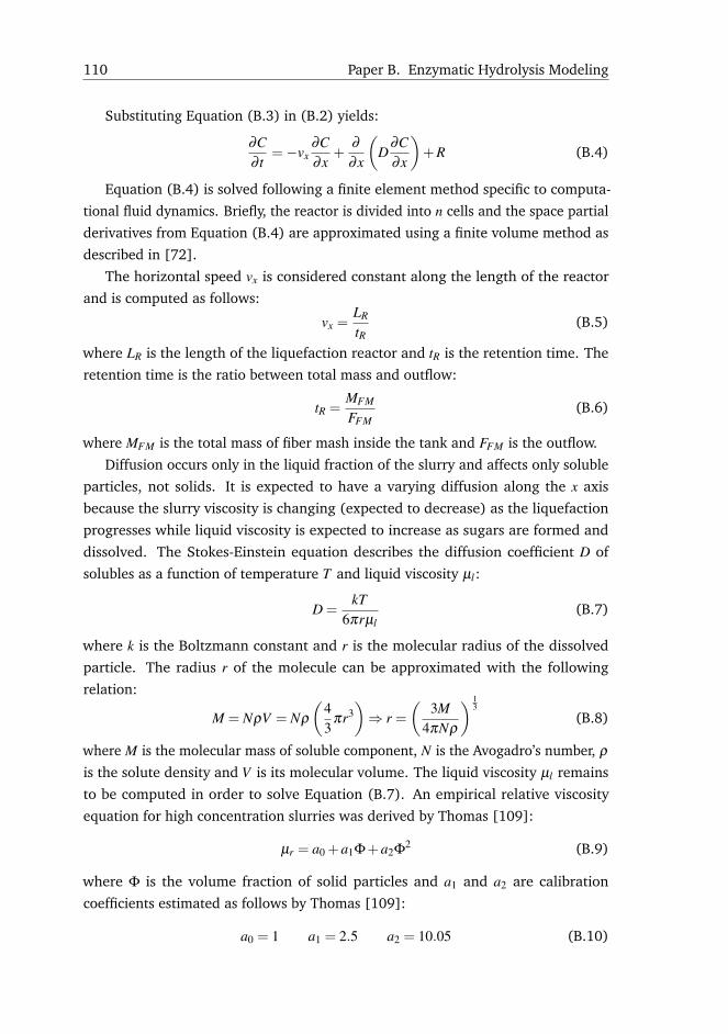
110 Paper B. Enzymatic Hydrolysis Modeling
Substituting Equation (B.3) in (B.2) yields:
∂C∂ t
=−vx∂C∂x
+∂∂x
(D
∂C∂x
)+R (B.4)
Equation (B.4) is solved following a finite element method specific to computa-
tional fluid dynamics. Briefly, the reactor is divided into n cells and the space partial
derivatives from Equation (B.4) are approximated using a finite volume method as
described in [72].
The horizontal speed vx is considered constant along the length of the reactor
and is computed as follows:
vx =LR
tR(B.5)
where LR is the length of the liquefaction reactor and tR is the retention time. The
retention time is the ratio between total mass and outflow:
tR =MFM
FFM(B.6)
where MFM is the total mass of fiber mash inside the tank and FFM is the outflow.
Diffusion occurs only in the liquid fraction of the slurry and affects only soluble
particles, not solids. It is expected to have a varying diffusion along the x axis
because the slurry viscosity is changing (expected to decrease) as the liquefaction
progresses while liquid viscosity is expected to increase as sugars are formed and
dissolved. The Stokes-Einstein equation describes the diffusion coefficient D of
solubles as a function of temperature T and liquid viscosity µl:
D =kT
6πrµl(B.7)
where k is the Boltzmann constant and r is the molecular radius of the dissolved
particle. The radius r of the molecule can be approximated with the following
relation:
M = NρV = Nρ(
43
πr3)⇒ r =
(3M
4πNρ
) 13
(B.8)
where M is the molecular mass of soluble component, N is the Avogadro’s number, ρis the solute density and V is its molecular volume. The liquid viscosity µl remains
to be computed in order to solve Equation (B.7). An empirical relative viscosity
equation for high concentration slurries was derived by Thomas [109]:
µr = a0 +a1Φ+a2Φ2 (B.9)
where Φ is the volume fraction of solid particles and a1 and a2 are calibration
coefficients estimated as follows by Thomas [109]:
a0 = 1 a1 = 2.5 a2 = 10.05 (B.10)

B.3. Model Development 111
The relative viscosity µr and the liquid viscosity µl can then be used to compute
the slurry viscosity µs:
µs = µrµl (B.11)
As glucose is produced and dissolved in the liquid part of the slurry, the liquid
viscosity changes following a simple linear relation as given by Converti et al. [110]:
µl = µW +CGkGµ (B.12)
where µW is the viscosity of the pure liquid solvent, CG is the glucose concentration
and kGµ is a correlation parameter for glucose. kGµ and µW follow an empirical
exponential law also known as the Guzman-Andrade equation [111]:
µW = AW eBWT kGµ = AGe
BGT (B.13)
where AW and BW are fitting parameters for pure liquid, T is the reactor temperature,
and AG and BG are parameters for sugar correlation. µW is approximately water
viscosity and numerical values for AW , BW , AG and BG are given by Converti et al.
[110]:
AW = 2.41×10⁻³ gm−1 s−1
BW = 1774.9K
AG = 8.65×10⁻¹⁰ m2 s−1
BG = 2502K
(B.14)
B.3.3 pH Modeling
The pH model is an extension of the model presented in an earlier publication
[12] and comprises a set of 8 weak acids and strong base hydration reactions: self-
ionization of water (Equation (B.15c)), acetic acid dissociation (Equation (B.15a)),
carbonic acid formation and dissociation (Equations (B.15d) and (B.15e)), succinic
acid dissociation (Equations (B.15f) and (B.15g)) and lactic acid dissociation (Equa-
tion (B.15h)). The hydration equations are modeled using the approach described
by McAvoy et al. [112]. The complete set of equilibrium dissociation equations is
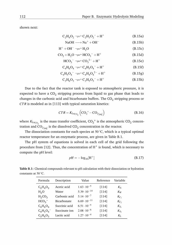
112 Paper B. Enzymatic Hydrolysis Modeling
shown next:
C2H4O2 ↽−−−⇀ C2H3O −2 +H+ (B.15a)
NaOH−−→ Na++OH− (B.15b)
H++OH− ↽−−−⇀ H2O (B.15c)
CO2 +H2O ↽−−−⇀ HCO −3 +H+ (B.15d)
HCO −3 ↽−−−⇀ CO 2−
3 +H+ (B.15e)
C4H6O4 ↽−−−⇀ C4H5O −4 +H+ (B.15f)
C4H5O −4 ↽−−−⇀ C4H4O 2−
4 +H+ (B.15g)
C3H6O3 ↽−−−⇀ C3H5O −3 +H+ (B.15h)
Due to the fact that the reactor tank is exposed to atmospheric pressure, it is
expected to have a CO2 stripping process from liquid to gas phase that leads to
changes in the carbonic acid and bicarbonate buffers. The CO2 stripping process or
CT R is modeled as in [113] with typical saturation kinetics:
CT R = KLaCO2
(CO ∗
2 −CO2[aq]
)(B.16)
where KLaCO2is the mass transfer coefficient, CO *2 is the atmospheric CO2 concen-
tration and CO2[aq] is the dissolved CO2 concentration in the reactor.
The dissociation constants for each species at 50 ◦C, which is a typical optimal
reactor temperature for an enzymatic process, are given in Table B.1.
The pH system of equations is solved in each cell of the grid following the
procedure from [12]. Thus, the concentration of H+ is found, which is necessary to
compute the pH level:
pH =− log10[H+] (B.17)
Table B.1: Chemical compounds relevant to pH calculation with their dissociation or hydration
constants at 50 ◦C.
Formula Description Value Reference Variable
C2H4O2 Acetic acid 1.63 ·10−5 [114] KA
H2O Water 5.39 ·10−14 [114] KW
H2CO3 Carbonic acid 5.14 ·10−7 [114] KC1
HCO –3 Bicarbonate 6.69 ·10−11 [114] KC2
C4H6O4 Succinic acid 6.51 ·10−5 [114] KS1
C4H5O –4 Succinate ion 2.08 ·10−6 [114] KS2
C3H6O3 Lactic acid 1.27 ·10−4 [114] KL
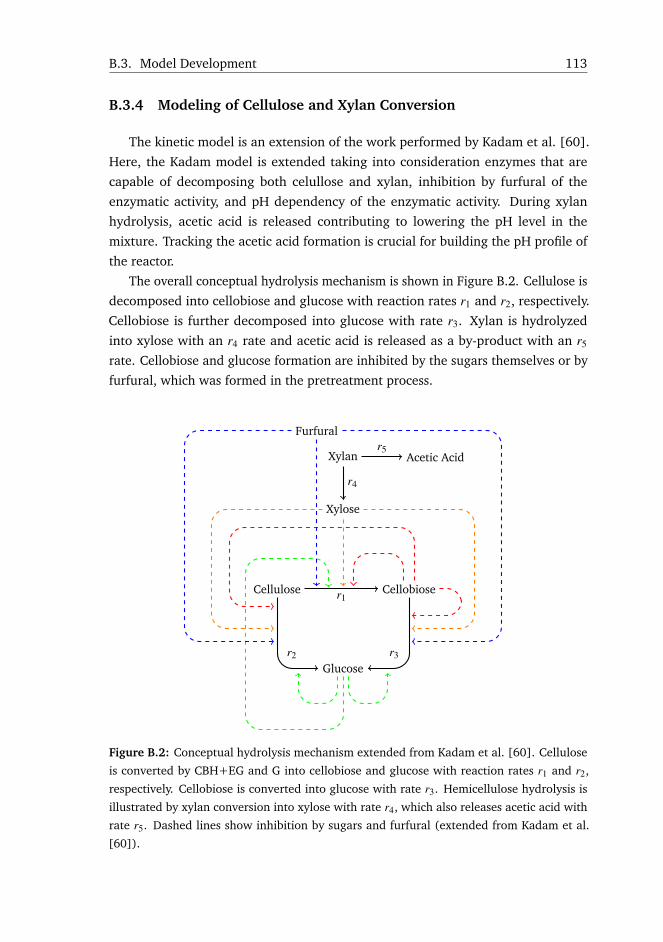
B.3. Model Development 113
B.3.4 Modeling of Cellulose and Xylan Conversion
The kinetic model is an extension of the work performed by Kadam et al. [60].
Here, the Kadam model is extended taking into consideration enzymes that are
capable of decomposing both celullose and xylan, inhibition by furfural of the
enzymatic activity, and pH dependency of the enzymatic activity. During xylan
hydrolysis, acetic acid is released contributing to lowering the pH level in the
mixture. Tracking the acetic acid formation is crucial for building the pH profile of
the reactor.
The overall conceptual hydrolysis mechanism is shown in Figure B.2. Cellulose is
decomposed into cellobiose and glucose with reaction rates r1 and r2, respectively.
Cellobiose is further decomposed into glucose with rate r3. Xylan is hydrolyzed
into xylose with an r4 rate and acetic acid is released as a by-product with an r5
rate. Cellobiose and glucose formation are inhibited by the sugars themselves or by
furfural, which was formed in the pretreatment process.
Cellulose Cellobiose
Glucose
Xylan
Xylose
Furfural
Acetic Acid
r1
r2 r3
r4
r5
Figure B.2: Conceptual hydrolysis mechanism extended from Kadam et al. [60]. Cellulose
is converted by CBH+EG and G into cellobiose and glucose with reaction rates r1 and r2,
respectively. Cellobiose is converted into glucose with rate r3. Hemicellulose hydrolysis is
illustrated by xylan conversion into xylose with rate r4, which also releases acetic acid with
rate r5. Dashed lines show inhibition by sugars and furfural (extended from Kadam et al.
[60]).

114 Paper B. Enzymatic Hydrolysis Modeling
The following chemical species are tracked in the conversion model:
CK =[
CCS CXS CLS CC CG CX CF CE
]>(B.18)
where CCS , CXS and CLS are solid components from the slurry, i.e. cellulose, xylan and
lignin concentrations, and CC, CG, CX , CF and CE constitute the liquid part of the
slurry, i.e. cellobiose, glucose, xylose, furfural and enzymes, respectively. Equation
(B.4) is evaluated for each species from Equation (B.18). The boundary conditions
of Equation (B.4) are constructed from the initial chemical composition of pretreated
fibers, or CK0 , which is measured in reality with NIR equipment.
The enzymes cocktail is a complex mixture containing many protein types that
could be divided into cellulase, hemicellulase and other type of proteins. Cel-
lulose is hydrolyzed by the cellulase group, which is subdivided into exo-β -1.4-
cellobiohydrolase and endo-β -1.4-glucanase (CBH+EG), notated as CE1 , and β -
glucosidase (G) enzymes, i.e. CE2 . Xylan is hydrolyzed by the hemicellulase (X)
group, i.e. CE3 . There are other types of enzymes in the mixture in negligible
amounts and their concentration is notated as CE4 . The enzymatic cocktail can then
be parametrized in αi with i from 1 to 4 representing the fraction of each enzyme
type. The total enzyme concentration can then be expressed as the sum of each
enzyme concentration:
CE =CE1 +CE2 +CE3 +CE4 (B.19)
There is an equilibrium between bounded and free enzymes, which is simplified
to the following equation:
EnzymeF +Solids←−→ Enzyme−SolidsB (B.20)
where EnzymeF are free enzymes and Enzyme-SolidsB are bounded enzymes to
solids. Therefore, enzymes can be in one of the two states: bounded to solids (B) or
free (F). The total concentration of CBH+EG, G or X enzymes consists of bounded
and free enzymes:
CEi =CEiB+CEiF
(B.21)
where i = 1,2,3. The effects of the other type of enzymes, i.e. i = 4, is neglected as
they do not participate actively to cellulose and xylan decomposition.
The equilibrium between adsorbed and free enzymes follows a Langmuir isotherm
expression. In the case of type i enzymes, where i can be CBH+EG, G or X, the
Langmuir isotherm relation expresses the ratio between concentration of adsorbed
enzymes and solids:CEiB
CS= EMi
KAiCEiF
1+KAiCEiF
(B.22)
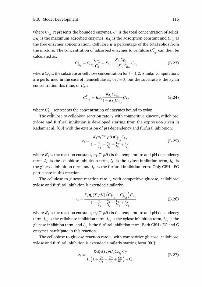
B.3. Model Development 115
where CEiBrepresents the bounded enzymes, CS is the total concentration of solids,
EMi is the maximum adsorbed enzymes, KAi is the adsorption constant and CEiFis
the free enzymes concentration. Cellulose is a percentage of the total solids from
the mixture. The concentration of adsorbed enzymes to cellulose CCEiB
can then be
calculated as:
CCEiB
=CEiB
CCS
CS= EMi
KAiCEiF
1+KAiCEiF
CCS (B.23)
where CCS is the substrate or cellulose concentration for i= 1,2. Similar computations
are performed in the case of hemicellulases, or i = 3, but the substrate is the xylan
concentration this time, or CXS :
CXE3B
= EM3
KA3CE3F
1+KA3CE3F
CXS (B.24)
where CXE3B
represents the concentration of enzymes bound to xylan.
The cellulose to cellobiose reaction rate r1 with competitive glucose, cellobiose,
xylose and furfural inhibition is developed starting from the expression given in
Kadam et al. [60] with the extension of pH dependency and furfural inhibition:
r1 =K1η1(T, pH)CC
E1BCCS
1+ CCIC1
+ CXIX1
+ CGIG1
+ CFIF1
(B.25)
where K1 is the reaction constant, η1(T, pH) is the temperature and pH dependency
term, IC1 is the cellobiose inhibition term, IX1 is the xylose inhibition term, IG1 is
the glucose inhibition term, and IF1 is the furfural inhibition term. Only CBH+EG
participate in this reaction.
The cellulose to glucose reaction rate r2 with competitive glucose, cellobiose,
xylose and furfural inhibition is extended similarly:
r2 =K2η2(T, pH)
(CC
E1B+CC
E2B
)CCS
1+ CCIC2
+ CXIX2
+ CGIG2
+ CFIF2
(B.26)
where K2 is the reaction constant, η2(T, pH) is the temperature and pH dependency
term, IC2 is the cellobiose inhibition term, IX2 is the xylose inhibition term, IG2 is the
glucose inhibition term, and IF2 is the furfural inhibition term. Both CBH+EG and G
enzymes participate in this reaction.
The cellobiose to glucose reaction rate r3 with competitive glucose, cellobiose,
xylose and furfural inhibition is extended similarly starting form [60]:
r3 =K3η3(T, pH)CE2F
CC
I3
(1+ CX
IX3+ CG
IG3+ CF
IF3
)+CC
(B.27)
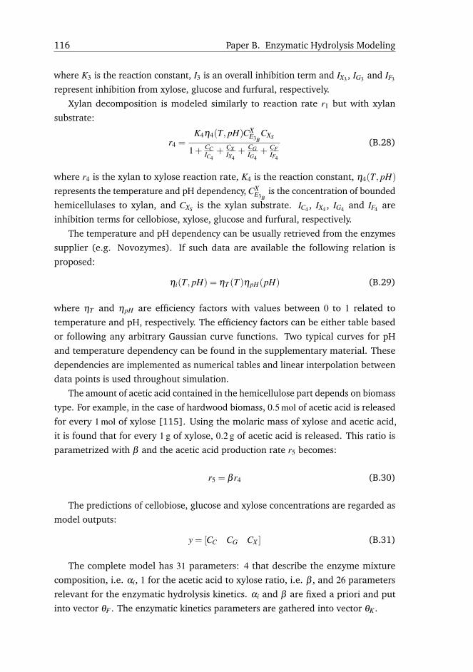
116 Paper B. Enzymatic Hydrolysis Modeling
where K3 is the reaction constant, I3 is an overall inhibition term and IX3 , IG3 and IF3
represent inhibition from xylose, glucose and furfural, respectively.
Xylan decomposition is modeled similarly to reaction rate r1 but with xylan
substrate:
r4 =K4η4(T, pH)CX
E3BCXS
1+ CCIC4
+ CXIX4
+ CGIG4
+ CFIF4
(B.28)
where r4 is the xylan to xylose reaction rate, K4 is the reaction constant, η4(T, pH)
represents the temperature and pH dependency, CXE3B
is the concentration of bounded
hemicellulases to xylan, and CXS is the xylan substrate. IC4 , IX4 , IG4 and IF4 are
inhibition terms for cellobiose, xylose, glucose and furfural, respectively.
The temperature and pH dependency can be usually retrieved from the enzymes
supplier (e.g. Novozymes). If such data are available the following relation is
proposed:
ηi(T, pH) = ηT (T )ηpH(pH) (B.29)
where ηT and ηpH are efficiency factors with values between 0 to 1 related to
temperature and pH, respectively. The efficiency factors can be either table based
or following any arbitrary Gaussian curve functions. Two typical curves for pH
and temperature dependency can be found in the supplementary material. These
dependencies are implemented as numerical tables and linear interpolation between
data points is used throughout simulation.
The amount of acetic acid contained in the hemicellulose part depends on biomass
type. For example, in the case of hardwood biomass, 0.5 mol of acetic acid is released
for every 1 mol of xylose [115]. Using the molaric mass of xylose and acetic acid,
it is found that for every 1 g of xylose, 0.2 g of acetic acid is released. This ratio is
parametrized with β and the acetic acid production rate r5 becomes:
r5 = β r4 (B.30)
The predictions of cellobiose, glucose and xylose concentrations are regarded as
model outputs:
y = [CC CG CX ] (B.31)
The complete model has 31 parameters: 4 that describe the enzyme mixture
composition, i.e. αi, 1 for the acetic acid to xylose ratio, i.e. β , and 26 parameters
relevant for the enzymatic hydrolysis kinetics. αi and β are fixed a priori and put
into vector θF . The enzymatic kinetics parameters are gathered into vector θK .
B.3. Model Development 117
B.3.5 Model Calibration, Sensitivity and Uncertainty Analysis
The previous analysis of the Kadam model performed by Sin et al. [8] indicated
that the model was over parameterized with respect to available measurements.
Hence, for a proper model calibration, a sensitivity analysis was performed to find
out the most significant parameters to be used as subset for fine tuning of the model
fits to the available data. The sensitivity analysis is conducted by calculating a
measure called δ msqrk as in the methodology described in [64]:
δ msqrk =
√1N
N
∑i=1
(snd,ik
)(B.32)
where k is the parameter index in the hydrolysis parameter vector θK , i is the model
output index and snd,ik is the non dimensional sensitivity defined as:
snd,ik =∂yi
∂θk
θk
sci(B.33)
where ∂yi/∂θk represents the output variation with respect to a variation in pa-
rameter θk and sci is a scaling factor with the same physical dimension as the
corresponding observation. All parameters are ranked according to δ msqrk and a
subset θS is built with the most significant parameters.
A model calibration follows, which adjusts the parameters from the θS subset in
order to obtain a better fit. For this calibration, only 50 h out of the 170 h of recorded
data are used, while the remaining 120 h data are used for validation. It is noted
that the calibration of the model parameters is meant to be a fine-tuning around
the nominal values of the model parameters estimated from batch assays by Kadam
et al. [60]. A comprehensive system identification is not pursued due to the fact that
available plant measurements were obtained from closed loop operation and not
under proper optimal experimental design.
Uncertainty Analysis
The uncertainty analysis is carried out using the engineering standard Monte
Carlo technique, which includes the following four steps [9]: (1) define input
uncertainties with their range; (2) sampling of kinetics and feed parameters using the
Latin hypercube sampling with correlation control; (3) run Monte Carlo simulations
with sampled values; (4) evaluate results. In the last step, in addition to inference
statistics, a sensitivity analysis was also performed using linear regression of Monte
Carlo outputs, also known as the standardized regression coefficients (SRC). The
methodology is detailed in [9].
In step 1, the uncertainty analysis considers two sources of uncertainty, namely
kinetic parameters and feed composition (mass). For definition of the kinetic
118 Paper B. Enzymatic Hydrolysis Modeling
parameter uncertainty, a uniform distribution with the corresponding lower and
upper bounds are used as defined in [9], while the correlation matrix between the
parameters was taken from [8]. Bias and standard deviation of measurements due
to sensors were considered for the characterization of feed composition uncertainty.
The feed measurements are subject to errors either due to a miss calibration of the
NIR equipment or because of a wrongly placed sensor, which often indicates offsets
in the mass inflow of fibers. The most relevant feed variables are cellulose and xylan
content, and fiber mass inflow. The error that affects these signals are statistically
characterized using normal distributions with the following parameters:
εC ∈ N(µC,σ2C) εX ∈ N(µX ,σ2
X ) εF ∈ N(µF ,σ2F) (B.34)
where εC, εX and εF are cellulose, xylan and inflow errors, and N is the normal
distribution. The mean values µC, µX and µF represent sensor offsets and are
normally distributed such that to cover a range of 5 % to 10 % of their nominal
operational values, an error range assumed for NIR equipments. The standard
deviations of the measurements are considered to follow gamma distributions, which
is good practice in measurement error modeling. Hence the uncertainty on the
measured feed composition are generated by performing LHS on 2 parameters of
the normal distribution: one that characterizes the probability of the mean value,
notated as Fµ , and another one for the standard deviation, i.e. Fσ .
The SRC method fits a linear regression model to Monte Carlo simulation outputs
[65]:
yreg = b0 +Nθ
∑i=1
biθi (B.35)
where θi is the uncertain parameter vector of length Nθ , bi are the regression
coefficients and yreg is the fitted model output. The regression coefficients bi are then
scaled with respect to the standard deviation in parameters and simulation outputs:
βi =σθi
σybi (B.36)
where βi are the standardized regression coefficients, σθi is the standard deviation
of parameter uncertainty and σy is the simulation output standard deviation.
B.3.6 Simulation Scenarios
The model is evaluated in two different scenarios: the first one concerns a steady-
state average performance simulation while in the second one the model is driven by
real measurements and its predictions are compared against HPLC data throughout
170 h of operation.

B.4. Results and Discussion 119
In the first scenario, the reactor is assumed to be filled initially with water and all
model inputs, including feed composition, are set to a typical operational point of a
demonstration scale biorefinery as in Table B.2. The reactor is capable of processing
4 th−1 of fibers. Water and enzymes inflows are adjusted proportionally to fibers
inflow. A mass controller automatically sets the outflow of fiber mash in order to
keep a constant holdup. The purpose of this scenario is to observe the steady-state
concentrations, pH, viscosity and solids profiles from the reactor.
Table B.2: Dry matter composition of steam pretreated wheat straw at 170 ◦C: demonstration
scale plant values against composition determined by [116].
Component Demonstration Plant [116]
Cellulose 45.0 % 50.0 %
Xylan 10.0 % 13.6 %
Lignin 32.0 % 20.8 %
Other 13.0 % 15.6 %
B.4 Results and Discussion
B.4.1 Model Sensitivity and Calibration
Model parameters are initialized to reported values from [60], which are given
in Table B.3. There are a few missing parameters referring to xylan hydrolysis and
furfural inhibition, which have not been reported earlier in the literature. These
parameters are initialized to reasonable values.
The δ msqr sensitivity measure is numerically computed for each output as δ msqrC ,
δ msqrG and δ msqr
X , representing cellobiose, glucose and xylose, respectively, and also
as an overall indicator δ msqr. Parameters are ranked with respect to δ msqr and the
results are shown in Figure B.3. As expected, the model is over parametrized and
only a subset of parameters is relevant for the output dynamics. A threshold for
δ msqr is set to 0.025 in this case (there is no absolute threshold value reported [8])
and shown in the bottom plot of Figure B.3. The subset of significant parameters is
found as follows:
θS = [K1 K2 K4 EM1 KA1 IC1 IG1 IX1 IG2 IX2 IG4 ]> (B.37)
The sensitivity analysis results indicate that the reaction rates that participate
in cellobiose, glucose and xylose formation, i.e. K1, K2 and K4, are influential
parameters. Inhibition of r1 and r2 by glucose and xylose, i.e. IG1 , IG2 , IX1 and IX2 , as
well as IG4 or inhibition of r4 by glucose, and IC1 or inhibition of r1 by cellobiose, also
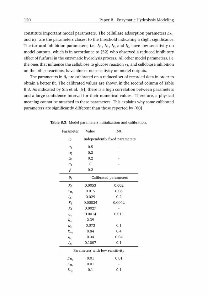
120 Paper B. Enzymatic Hydrolysis Modeling
constitute important model parameters. The cellullase adsorption parameters EM1
and KA1 are the parameters closest to the threshold indicating a slight significance.
The furfural inhibition parameters, i.e. IF1 , IF2 , IF3 and IF4 have low sensitivity on
model outputs, which is in accordance to [52] who observed a reduced inhibitory
effect of furfural in the enzymatic hydrolysis process. All other model parameters, i.e.
the ones that influence the cellobiose to glucose reaction r3, and cellobiose inhibition
on the other reactions, have almost no sensitivity on model outputs.
The parameters in θS are calibrated on a reduced set of recorded data in order to
obtain a better fit. The calibrated values are shown in the second column of Table
B.3. As indicated by Sin et al. [8], there is a high correlation between parameters
and a large confidence interval for their numerical values. Therefore, a physical
meaning cannot be attached to these parameters. This explains why some calibrated
parameters are significantly different than those reported by [60].
Table B.3: Model parameters initialization and calibration.
Parameter Value [60]
θF Independently fixed parameters
α1 0.5 -
α2 0.3 -
α3 0.2 -
α4 0 -
β 0.2 -
θS Calibrated parameters
K2 0.0053 0.002
EM1 0.015 0.06
IX2 0.029 0.2
K1 0.00034 0.0062
K4 0.0027 -
IC1 0.0014 0.015
IG4 2.39 -
IG1 0.073 0.1
KA1 0.84 0.4
IG2 0.34 0.04
IX1 0.1007 0.1
Parameters with low sensitivity
EM2 0.01 0.01
EM3 0.01 -
KA2 0.1 0.1
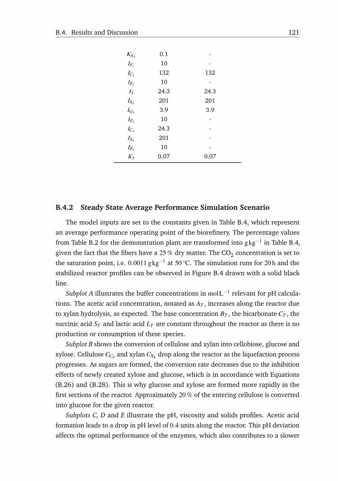
B.4. Results and Discussion 121
KA3 0.1 -
IF1 10 -
IC2 132 132
IF2 10 -
I3 24.3 24.3
IX3 201 201
IG3 3.9 3.9
IF3 10 -
IC4 24.3 -
IX4 201 -
IF4 10 -
K3 0.07 0.07
B.4.2 Steady State Average Performance Simulation Scenario
The model inputs are set to the constants given in Table B.4, which represent
an average performance operating point of the biorefinery. The percentage values
from Table B.2 for the demonstration plant are transformed into gkg−1 in Table B.4,
given the fact that the fibers have a 25 % dry matter. The CO2 concentration is set to
the saturation point, i.e. 0.0011 gkg−1 at 50 ◦C. The simulation runs for 20 h and the
stabilized reactor profiles can be observed in Figure B.4 drawn with a solid black
line.
Subplot A illustrates the buffer concentrations in molL−1 relevant for pH calcula-
tions. The acetic acid concentration, notated as AT , increases along the reactor due
to xylan hydrolysis, as expected. The base concentration BT , the bicarbonate CT , the
succinic acid ST and lactic acid LT are constant throughout the reactor as there is no
production or consumption of these species.
Subplot B shows the conversion of cellulose and xylan into cellobiose, glucose and
xylose. Cellulose CCS and xylan CXS drop along the reactor as the liquefaction process
progresses. As sugars are formed, the conversion rate decreases due to the inhibition
effects of newly created xylose and glucose, which is in accordance with Equations
(B.26) and (B.28). This is why glucose and xylose are formed more rapidly in the
first sections of the reactor. Approximately 20 % of the entering cellulose is converted
into glucose for the given reactor.
Subplots C, D and E illustrate the pH, viscosity and solids profiles. Acetic acid
formation leads to a drop in pH level of 0.4 units along the reactor. This pH deviation
affects the optimal performance of the enzymes, which also contributes to a slower
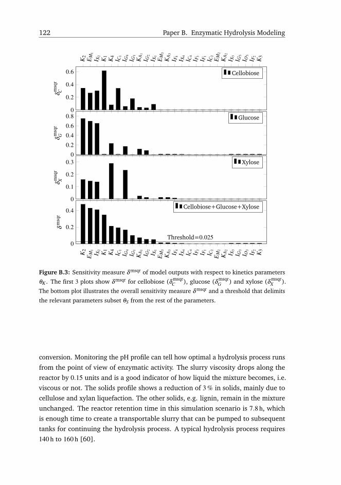
122 Paper B. Enzymatic Hydrolysis Modeling
K2
EM
1
I X2
K1
K4
I C1
I G4
I G1
KA
1
I G2
I X1
EM
3
KA
3
I F4
I X4
I C4
I F3
I F1
I C2
EM
2
KA
2
I X3
I G3
I O3
I F2
K3
0
0.2
0.4
0.6
δmsq
rC
Cellobiose
0
0.2
0.4
0.6
0.8
δmsq
rG
Glucose
0
0.1
0.2
0.3
δmsq
rX
Xylose
K2
EM
1
I X2
K1
K4
I C1
I G4
I G1
KA
1
I G2
I X1
EM
3
KA
3
I F4
I X4
I C4
I F3
I F1
I C2
EM
2
KA
2
I X3
I G3
I O3
I F2
K3
0
0.2
0.4
Threshold=0.025
δmsq
r
Cellobiose+Glucose+Xylose
Figure B.3: Sensitivity measure δ msqr of model outputs with respect to kinetics parameters
θK . The first 3 plots show δ msqr for cellobiose (δ msqrC ), glucose (δ msqr
G ) and xylose (δ msqrX ).
The bottom plot illustrates the overall sensitivity measure δ msqr and a threshold that delimits
the relevant parameters subset θS from the rest of the parameters.
conversion. Monitoring the pH profile can tell how optimal a hydrolysis process runs
from the point of view of enzymatic activity. The slurry viscosity drops along the
reactor by 0.15 units and is a good indicator of how liquid the mixture becomes, i.e.
viscous or not. The solids profile shows a reduction of 3 % in solids, mainly due to
cellulose and xylan liquefaction. The other solids, e.g. lignin, remain in the mixture
unchanged. The reactor retention time in this simulation scenario is 7.8 h, which
is enough time to create a transportable slurry that can be pumped to subsequent
tanks for continuing the hydrolysis process. A typical hydrolysis process requires
140 h to 160 h [60].
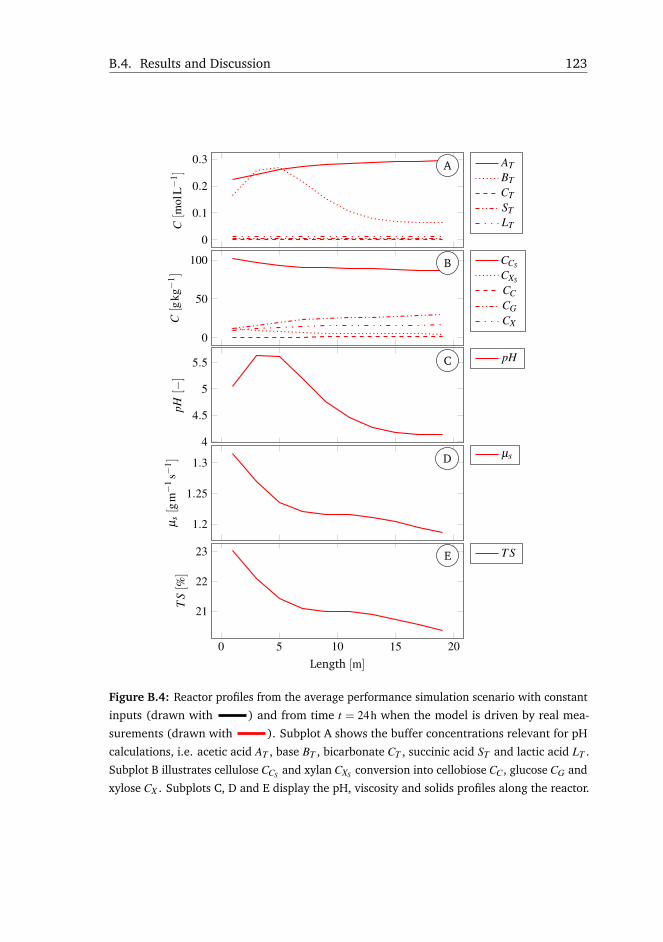
B.4. Results and Discussion 123
0
0.1
0.2
0.3 AC[m
olL−
1 ]ATBTCTSTLT
0
50
100 B
C[g
kg−
1 ]
CCS
CXS
CCCGCX
4
4.5
5
5.5 C
pH[−
]
pH
1.2
1.25
1.3 D
µ s[g
m−
1s−
1 ]
µs
0 5 10 15 20
21
22
23 E
Length [m]
TS[%
]
T S
Figure B.4: Reactor profiles from the average performance simulation scenario with constant
inputs (drawn with ) and from time t = 24h when the model is driven by real mea-
surements (drawn with ). Subplot A shows the buffer concentrations relevant for pH
calculations, i.e. acetic acid AT , base BT , bicarbonate CT , succinic acid ST and lactic acid LT .
Subplot B illustrates cellulose CCS and xylan CXS conversion into cellobiose CC, glucose CG and
xylose CX . Subplots C, D and E display the pH, viscosity and solids profiles along the reactor.
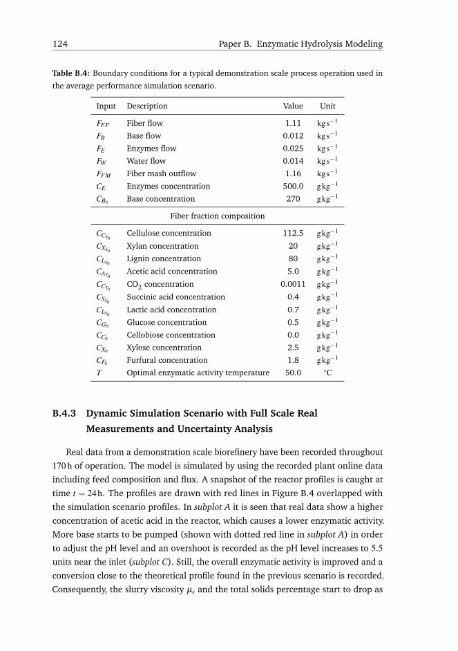
124 Paper B. Enzymatic Hydrolysis Modeling
Table B.4: Boundary conditions for a typical demonstration scale process operation used in
the average performance simulation scenario.
Input Description Value Unit
FFF Fiber flow 1.11 kgs−1
FB Base flow 0.012 kgs−1
FE Enzymes flow 0.025 kgs−1
FW Water flow 0.014 kgs−1
FFM Fiber mash outflow 1.16 kgs−1
CE Enzymes concentration 500.0 gkg−1
CB0 Base concentration 270 gkg−1
Fiber fraction composition
CCS0Cellulose concentration 112.5 gkg−1
CXS0Xylan concentration 20 gkg−1
CLS0Lignin concentration 80 gkg−1
CAT0Acetic acid concentration 5.0 gkg−1
CCT0CO2 concentration 0.0011 gkg−1
CST0Succinic acid concentration 0.4 gkg−1
CLT0Lactic acid concentration 0.7 gkg−1
CG0 Glucose concentration 0.5 gkg−1
CC0 Cellobiose concentration 0.0 gkg−1
CX0 Xylose concentration 2.5 gkg−1
CF0 Furfural concentration 1.8 gkg−1
T Optimal enzymatic activity temperature 50.0 ◦C
B.4.3 Dynamic Simulation Scenario with Full Scale Real
Measurements and Uncertainty Analysis
Real data from a demonstration scale biorefinery have been recorded throughout
170 h of operation. The model is simulated by using the recorded plant online data
including feed composition and flux. A snapshot of the reactor profiles is caught at
time t = 24h. The profiles are drawn with red lines in Figure B.4 overlapped with
the simulation scenario profiles. In subplot A it is seen that real data show a higher
concentration of acetic acid in the reactor, which causes a lower enzymatic activity.
More base starts to be pumped (shown with dotted red line in subplot A) in order
to adjust the pH level and an overshoot is recorded as the pH level increases to 5.5units near the inlet (subplot C). Still, the overall enzymatic activity is improved and a
conversion close to the theoretical profile found in the previous scenario is recorded.
Consequently, the slurry viscosity µs and the total solids percentage start to drop as

B.4. Results and Discussion 125
illustrated in subplots D and C. Conversion still occurs even though the hydrolysis
process runs suboptimal from the point of view of the enzymatic activity.
The top plot in Figure B.5 illustrates the outstream pH prediction, which fits rela-
tively well with the sensor data. There are several reasons that can cause estimation
differences: the online HPLC analyzer of pretreated fibers is the major source of
inaccuracies regarding the relevant buffer concentrations for pH calculations; the
flow measurement of fibers also presents drifts and offsets leading to an erroneous
calculation of the incoming acids affecting the estimated pH; estimation errors could
also occur due to unknown buffers created in the pretreatment process; a last source
of errors could be the pH sensor itself, which can have offsets if the cleaning proce-
dure is not followed properly. For example, it is suspected that the pH sensor has an
offset error between 90 h to 140 h because the pH measurement drops below 4 units,
which is unlikely to happen in reality. Also, the measurements in this time frame
are very noisy compared to the non-faulty case and there is a sudden change in the
measurement at approximately t = 140h, which can happen only if the sensor has
been cleaned at that specific time.
The pH estimation is more dynamic than the measurement, presenting several
spikes when the reactor holdup is changing but stays most of the time within 4 to 5pH units with an error below 1 unit, which is considered satisfactory knowing the
complexity of the chemical species in the slurry.
The bottom plot from Figure B.5 shows the calculated fiber mash viscosity or µS.
The values indicate a rather liquid mixture that can be pumped further to subsequent
tanks. Typically, the viscosity near the tank inlet is above 1.3 units as indicated in
subplot D from Figure B.4.
Throughout the operation of the biorefinery, samples were grabbed at the outflow
every 6 h. These samples were then analyzed with an HPLC device in the laboratory
in order to observe the sugar concentrations. Figure B.6 displays glucose, xylose and
cellobiose concentrations from the outstream, i.e. measurements with bullet points
and predicted values with solid lines. The gray area indicates the 5th-95th percentile
interval obtained after running the Monte Carlo simulations with LHS sampling on
kinetics and feed parameters as explained in the methodology. The sugar formation
fits fairly well within the 5th-95th percentile. Some differences appear when the
reactor holdup changes, which can be due to non trivial mixing effects that are not
captured well by the 1-D transport equation.
The SRC coefficients are summarized in Table B.5, where all kinetic and feed
parameters are ranked with respect to the βi coefficients. The ranking shows that
most of the model output uncertainty is explained by the uncertainties in the kinetic
parameters. The contribution of the feed composition uncertainties to the model
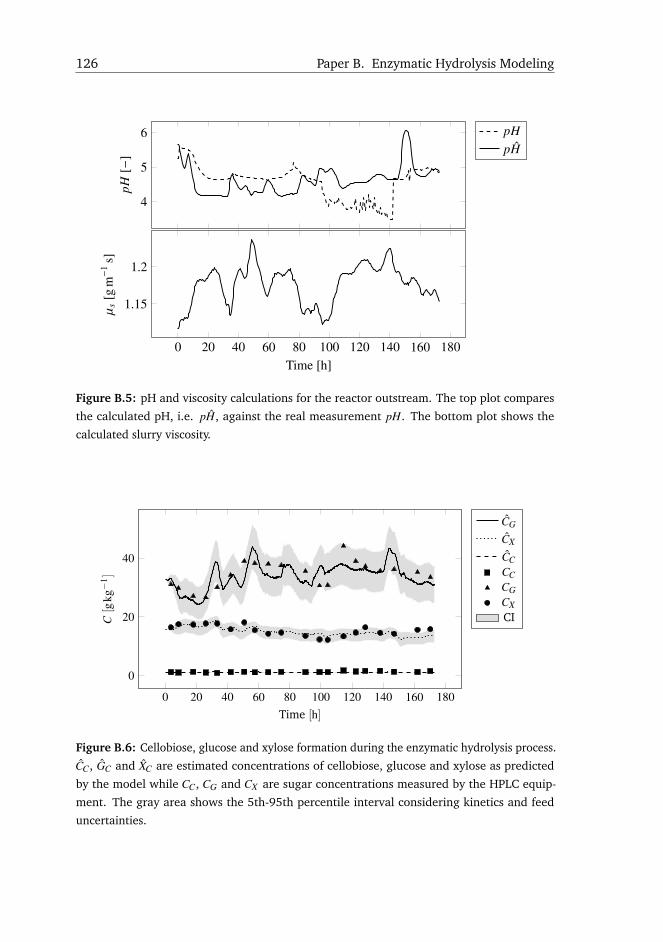
126 Paper B. Enzymatic Hydrolysis Modeling
4
5
6pH
[−]
pHpH
0 20 40 60 80 100 120 140 160 180
1.15
1.2
Time [h]
µs
[gm−1
s]
Figure B.5: pH and viscosity calculations for the reactor outstream. The top plot compares
the calculated pH, i.e. pH, against the real measurement pH. The bottom plot shows the
calculated slurry viscosity.
0 20 40 60 80 100 120 140 160 180
0
20
40
Time [h]
C[g
kg−
1 ]
CG
CX
CCCCCGCXCI
Figure B.6: Cellobiose, glucose and xylose formation during the enzymatic hydrolysis process.
CC, GC and XC are estimated concentrations of cellobiose, glucose and xylose as predicted
by the model while CC, CG and CX are sugar concentrations measured by the HPLC equip-
ment. The gray area shows the 5th-95th percentile interval considering kinetics and feed
uncertainties.
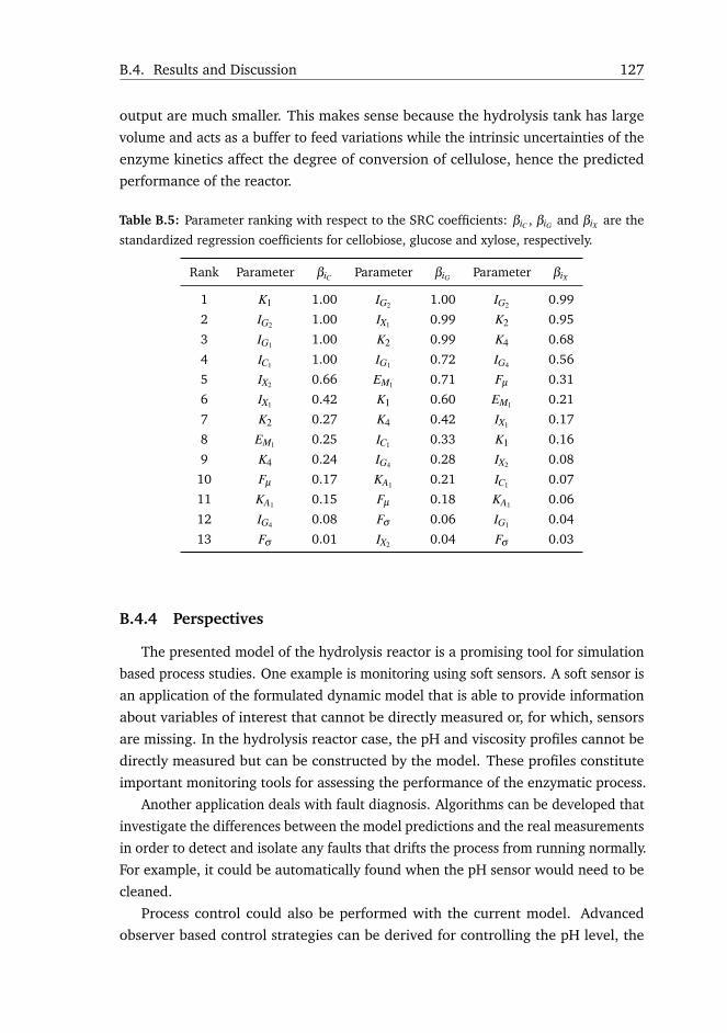
B.4. Results and Discussion 127
output are much smaller. This makes sense because the hydrolysis tank has large
volume and acts as a buffer to feed variations while the intrinsic uncertainties of the
enzyme kinetics affect the degree of conversion of cellulose, hence the predicted
performance of the reactor.
Table B.5: Parameter ranking with respect to the SRC coefficients: βiC , βiG and βiX are the
standardized regression coefficients for cellobiose, glucose and xylose, respectively.
Rank Parameter βiC Parameter βiG Parameter βiX
1 K1 1.00 IG2 1.00 IG2 0.99
2 IG2 1.00 IX1 0.99 K2 0.95
3 IG1 1.00 K2 0.99 K4 0.68
4 IC1 1.00 IG1 0.72 IG4 0.56
5 IX2 0.66 EM1 0.71 Fµ 0.31
6 IX1 0.42 K1 0.60 EM1 0.21
7 K2 0.27 K4 0.42 IX1 0.17
8 EM1 0.25 IC1 0.33 K1 0.16
9 K4 0.24 IG4 0.28 IX2 0.08
10 Fµ 0.17 KA1 0.21 IC1 0.07
11 KA1 0.15 Fµ 0.18 KA1 0.06
12 IG4 0.08 Fσ 0.06 IG1 0.04
13 Fσ 0.01 IX2 0.04 Fσ 0.03
B.4.4 Perspectives
The presented model of the hydrolysis reactor is a promising tool for simulation
based process studies. One example is monitoring using soft sensors. A soft sensor is
an application of the formulated dynamic model that is able to provide information
about variables of interest that cannot be directly measured or, for which, sensors
are missing. In the hydrolysis reactor case, the pH and viscosity profiles cannot be
directly measured but can be constructed by the model. These profiles constitute
important monitoring tools for assessing the performance of the enzymatic process.
Another application deals with fault diagnosis. Algorithms can be developed that
investigate the differences between the model predictions and the real measurements
in order to detect and isolate any faults that drifts the process from running normally.
For example, it could be automatically found when the pH sensor would need to be
cleaned.
Process control could also be performed with the current model. Advanced
observer based control strategies can be derived for controlling the pH level, the
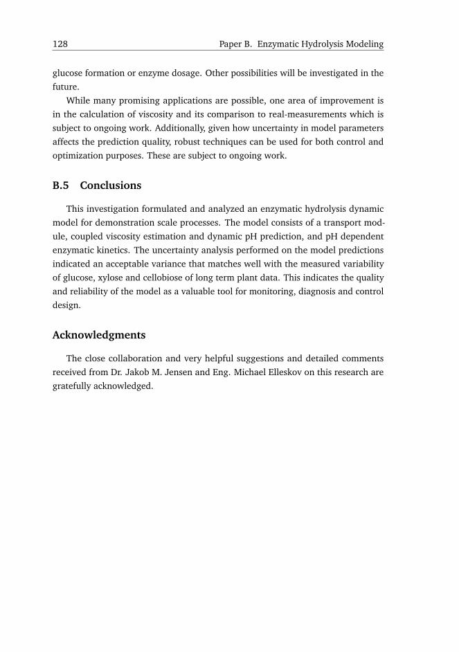
128 Paper B. Enzymatic Hydrolysis Modeling
glucose formation or enzyme dosage. Other possibilities will be investigated in the
future.
While many promising applications are possible, one area of improvement is
in the calculation of viscosity and its comparison to real-measurements which is
subject to ongoing work. Additionally, given how uncertainty in model parameters
affects the prediction quality, robust techniques can be used for both control and
optimization purposes. These are subject to ongoing work.
B.5 Conclusions
This investigation formulated and analyzed an enzymatic hydrolysis dynamic
model for demonstration scale processes. The model consists of a transport mod-
ule, coupled viscosity estimation and dynamic pH prediction, and pH dependent
enzymatic kinetics. The uncertainty analysis performed on the model predictions
indicated an acceptable variance that matches well with the measured variability
of glucose, xylose and cellobiose of long term plant data. This indicates the quality
and reliability of the model as a valuable tool for monitoring, diagnosis and control
design.
Acknowledgments
The close collaboration and very helpful suggestions and detailed comments
received from Dr. Jakob M. Jensen and Eng. Michael Elleskov on this research are
gratefully acknowledged.
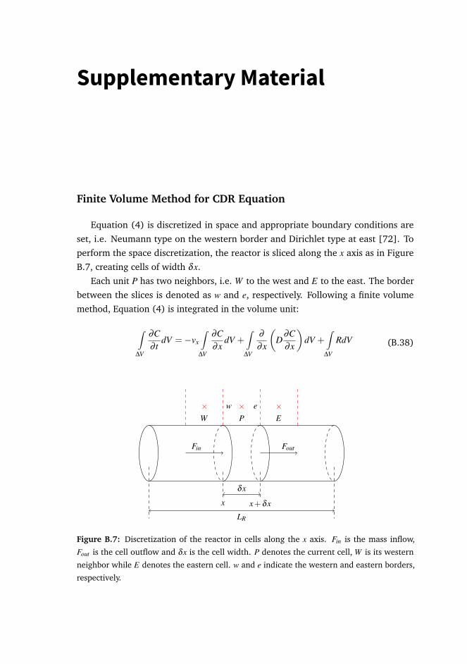
Supplementary Material
Finite Volume Method for CDR Equation
Equation (4) is discretized in space and appropriate boundary conditions are
set, i.e. Neumann type on the western border and Dirichlet type at east [72]. To
perform the space discretization, the reactor is sliced along the x axis as in Figure
B.7, creating cells of width δx.
Each unit P has two neighbors, i.e. W to the west and E to the east. The border
between the slices is denoted as w and e, respectively. Following a finite volume
method, Equation (4) is integrated in the volume unit:
∫∆V
∂C∂ t
dV =−vx
∫∆V
∂C∂x
dV +∫
∆V
∂∂x
(D
∂C∂x
)dV +
∫∆V
RdV (B.38)
δx
x x+δx
Fin Fout
w e×P
×W
×E
LR
Figure B.7: Discretization of the reactor in cells along the x axis. Fin is the mass inflow,
Fout is the cell outflow and δx is the cell width. P denotes the current cell, W is its western
neighbor while E denotes the eastern cell. w and e indicate the western and eastern borders,
respectively.
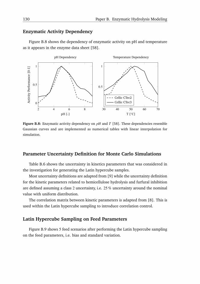
130 Paper B. Enzymatic Hydrolysis Modeling
Enzymatic Activity Dependency
Figure B.8 shows the dependency of enzymatic activity on pH and temperature
as it appears in the enzyme data sheet [58].
2 4 6 8
0
0.5
1
pH [-]
Act
ivit
yPe
rfor
man
ce[0
-1]
pH Dependency
30 40 50 60 70
0.5
1
T [◦C]
Temperature Dependency
Cellic CTec2Cellic CTec3
Figure B.8: Enzymatic activity dependency on pH and T [58]. These dependencies resemble
Gaussian curves and are implemented as numerical tables with linear interpolation for
simulation.
Parameter Uncertainty Definition for Monte Carlo Simulations
Table B.6 shows the uncertainty in kinetics parameters that was considered in
the investigation for generating the Latin hypercube samples.
Most uncertainty definitions are adapted from [9] while the uncertainty definition
for the kinetic parameters related to hemicellulose hydrolysis and furfural inhibition
are defined assuming a class 2 uncertainty, i.e. 25 % uncertainty around the nominal
value with uniform distribution.
The correlation matrix between kinetic parameters is adapted from [8]. This is
used within the Latin hypercube sampling to introduce correlation control.
Latin Hypercube Sampling on Feed Parameters
Figure B.9 shows 5 feed scenarios after performing the Latin hypercube sampling
on the feed parameters, i.e. bias and standard variation.
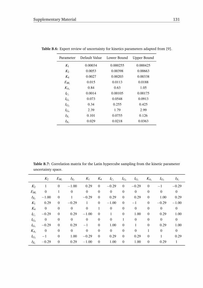
Supplementary Material 131
Table B.6: Expert review of uncertainty for kinetics parameters adapted from [9].
Parameter Default Value Lower Bound Upper Bound
K1 0.00034 0.000255 0.000425
K2 0.0053 0.00398 0.00663
K4 0.0027 0.00203 0.00338
EM1 0.015 0.0113 0.0188
KA1 0.84 0.63 1.05
IC1 0.0014 0.00105 0.00175
IG1 0.073 0.0548 0.0913
IG2 0.34 0.255 0.425
IG4 2.39 1.79 2.99
IX1 0.101 0.0755 0.126
IX2 0.029 0.0218 0.0363
Table B.7: Correlation matrix for the Latin hypercube sampling from the kinetic parameter
uncertainty space.
K2 EM1 IX2 K1 K4 IC1 IG4 IG1 KA1 IG2 IX1
K2 1 0 −1.00 0.29 0 −0.29 0 −0.29 0 −1 −0.29
EM1 0 1 0 0 0 0 0 0 0 0 0
IX2 −1.00 0 1 −0.29 0 0.29 0 0.29 0 1.00 0.29
K1 0.29 0 −0.29 1 0 −1.00 0 −1 0 −0.29 −1.00
K4 0 0 0 0 1 0 0 0 0 0 0
IC1 −0.29 0 0.29 −1.00 0 1 0 1.00 0 0.29 1.00
IG4 0 0 0 0 0 0 1 0 0 0 0
IG1 −0.29 0 0.29 −1 0 1.00 0 1 0 0.29 1.00
KA1 0 0 0 0 0 0 0 0 1 0 0
IG2 −1 0 1.00 −0.29 0 0.29 0 0.29 0 1 0.29
IX1 −0.29 0 0.29 −1.00 0 1.00 0 1.00 0 0.29 1
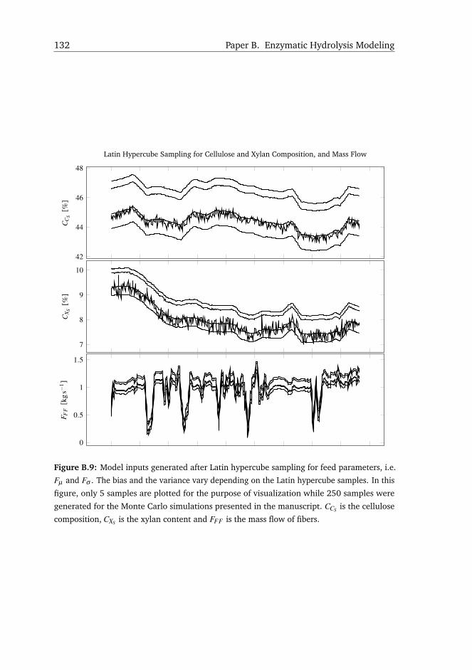
132 Paper B. Enzymatic Hydrolysis Modeling
42
44
46
48
CC
S[%
]
Latin Hypercube Sampling for Cellulose and Xylan Composition, and Mass Flow
7
8
9
10
CX S
[%]
0
0.5
1
1.5
F FF
[kg
s−1 ]
Figure B.9: Model inputs generated after Latin hypercube sampling for feed parameters, i.e.
Fµ and Fσ . The bias and the variance vary depending on the Latin hypercube samples. In this
figure, only 5 samples are plotted for the purpose of visualization while 250 samples were
generated for the Monte Carlo simulations presented in the manuscript. CCS is the cellulose
composition, CXS is the xylan content and FFF is the mass flow of fibers.
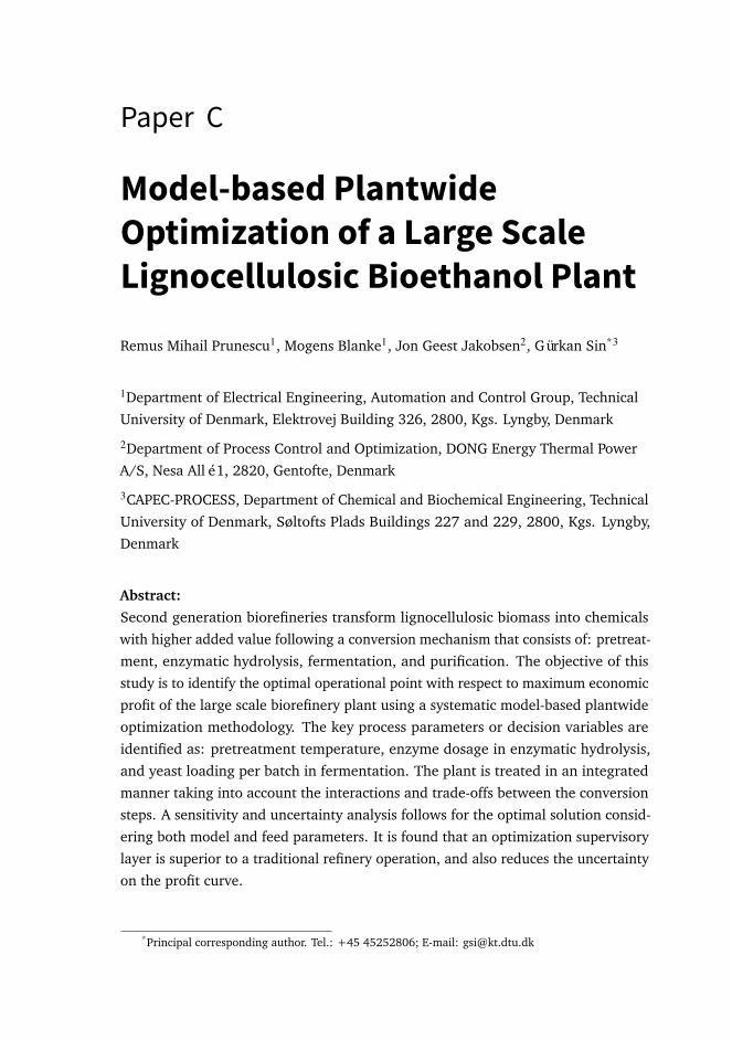
Paper C
Model-based PlantwideOptimization of a Large ScaleLignocellulosic Bioethanol Plant
Remus Mihail Prunescu1, Mogens Blanke1, Jon Geest Jakobsen2, Gürkan Sin*3
1Department of Electrical Engineering, Automation and Control Group, Technical
University of Denmark, Elektrovej Building 326, 2800, Kgs. Lyngby, Denmark
2Department of Process Control and Optimization, DONG Energy Thermal Power
A/S, Nesa Allé 1, 2820, Gentofte, Denmark
3CAPEC-PROCESS, Department of Chemical and Biochemical Engineering, Technical
University of Denmark, Søltofts Plads Buildings 227 and 229, 2800, Kgs. Lyngby,
Denmark
Abstract:
Second generation biorefineries transform lignocellulosic biomass into chemicals
with higher added value following a conversion mechanism that consists of: pretreat-
ment, enzymatic hydrolysis, fermentation, and purification. The objective of this
study is to identify the optimal operational point with respect to maximum economic
profit of the large scale biorefinery plant using a systematic model-based plantwide
optimization methodology. The key process parameters or decision variables are
identified as: pretreatment temperature, enzyme dosage in enzymatic hydrolysis,
and yeast loading per batch in fermentation. The plant is treated in an integrated
manner taking into account the interactions and trade-offs between the conversion
steps. A sensitivity and uncertainty analysis follows for the optimal solution consid-
ering both model and feed parameters. It is found that an optimization supervisory
layer is superior to a traditional refinery operation, and also reduces the uncertainty
on the profit curve.
*Principal corresponding author. Tel.: +45 45252806; E-mail: [email protected]

134 Paper C. Model-based Plantwide Optimization
C.1 Introduction
Second generation lignocellulosic biorefineries reached commercial reality in
2012 [3], and consequently many large scale plants are in operation nowadays: e.g.
Beta Renewables, Abengoa Bioenergy, GranBio, POET-DSM [2]. Most biorefineries
produce bioethanol but the drop in oil price reduced the demand on the biofuel.
However, plant upgrades for chemicals with higher-added values are recommended
making biorefineries still competitive in an oil dependent environment [26].
This study deals with optimizing the operation of a large scale second generation
biorefinery with a well established conversion route for bioethanol production using
modeling and simulation as enabling technology. The objective of the optimization
problem is to maximize the plant economical profit, considering prices for the most
important inputs and outputs: biomass, steam, enzymes, yeast, and ethanol among
others.
The conversion route from lignocellulosic material to products with higher added
value consists of: pretreatment, enzymatic hydrolysis, fermentation, and purification
[3, 4]. Lignocellulosic biomass contains cellulose, hemicellulose (xylan and arabi-
nan), lignin, ash, and other residues [37]. The scope of the pretreatment process is
to open the biomatrix, relocate lignin and partially hydrolyze the hemicellulose such
that cellulose would become more accessible to the downstream process of enzy-
matic hydrolysis [40]. During pretreatment, inhibitors such as organic acids, furfural,
and 5-Hydroxymethylfurfural (5-HMF) are also created due to sugar degradation.
Organic acids change the pH of medium, but can be automatically neutralized by a
pH controller for ensuring optimal enzymatic conditions [11]. Furfural, 5-HMF, and
acetate are fermentation inhibitors [52], while the remaining hemicellulose fraction
leads to xylooligomers and xylose formation in the enzymatic hydrolysis process,
which strongly inhibit the enzymatic activity [51].
There are trade-offs between the conversion steps. Too little biomass pretreat-
ment would reduce the exposed cellulose to enzymes, and also increases the amount
of hemicellulose for enzymatic hydrolysis, which would eventually decrease the
glucose yield due to xylose and xylooligomers inhibition. On the other hand, too
much biomass pretreatment would increase the amount of fermentation inhibitors
leading to a lower ethanol yield.
Most existing studies focus on operational optimization conducting small scale
experiments in the laboratory for finding the best pretreatment conditions such
that ethanol yield is maximized [50, 116, 117, 118]. The focus is on one unit at
a time (pretreatment versus enzymatic hydrolysis versus fermentation) but rarely
consider the steps simultaneously in an integrated manner. Such methods are time

C.2. Methods 135
consuming, suboptimal from an economic point of view as they do not take into
account process economics, and not suitable for large scale facilities. Also, in these
studies, the enzymatic hydrolysis and fermentation processes are usually conducted
following a fixed recipe, i.e. no correction action or feedback is taken to counteract
the effects of inhibitors. For example, one could increase the enzyme dosage when
xylooligomers and xylose inhibit glucose production, or adjust the yeast seed in
fermentation to compensate for inhibitors.
Therefore there is a need for systematic methods and tools to facilitate the
further process optimization and operation of second generation bioethanol plants,
which is the objective of this study. Moreover, the optimal solution proposed is also
analyzed from a sensitivity and uncertainty point of view with respect to feedstock
composition and kinetic parameters. A Monte Carlo technique with Latin Hypercube
Sampling and correlation control is used for the uncertainty analysis following the
methodology from [9, 66].
This paper is structured as follows: the methods section revises the methodology
for building the optimization layer for plantwide operation, along with the theoret-
ical part of the sensitivity and uncertainty analysis as well as the development of
necessary plant models. The results and discussion follow where the profit curve,
costs, and optimal solutions are presented along with their uncertainty bounds. The
paper concludes with a summary of all important findings.
C.2 Methods
C.2.1 Second Generation Bioethanol Plant
Figure C.1 illustrates the second generation biorefinery concept for bioethanol
production. The pretreatment process consists of a continuous thermal reactor and a
separation press, which were modeled and analyzed in [5, 71]. The thermal reactor
is equipped with a temperature controller for adjusting the reaction temperature
Ttr [12]. When hemicellulose is hydrolyzed, it produces xylose and arabinose (C5
sugars). After separation, the liquid part containing the C5 sugars is directly pumped
into fermentation reactors, bypassing the enzymatic hydrolysis reactors. Cellulose
can also be degraded in the pretreatment process, but the produced glucose (C6
sugar) is not lost as it is added to fermentation along with the C5 sugars from the
liquid fraction.
The enzymatic hydrolysis process was thoroughly described and analyzed in [6].
It runs at a high dry matter content in a continuous mode and consists of a series
of hydrolysis tanks. The first reactor is described in [54] followed by conventional
continuous stirred tank reactors in order to meet the necessary hydrolysis retention

136 Paper C. Model-based Plantwide Optimization
Figure C.1: Biorefinery diagram with assumed instrumentation. Pretreatment, the enzymatic
hydrolysis, and purification are continuous processes, while fermentation occurs in scheduled
batch reactors. Feedstock composition is assumed to be known, and can be measured in
reality with NIR equipment.
time of 140 h. The tanks are equipped with pH and temperature controllers in order
to keep optimal conditions for the enzymatic activity: e.g. pH = 5, and T = 50 ◦C[58]. Enzymes are added by a pump from a storage tank. The enzyme dosage Fe
can be adjusted accordingly and constitutes a degree of freedom in the optimization
problem.
The fermentation process runs in scheduled batch mode in a number of tanks
with a maximum holdup of 250 m3. The fermentation tanks have pH and temperature
controllers. Each batch consists of an inoculum phase, the fed-batch phase (which
cannot be neglected because it takes 60 h to fill the tank, time when reactions already
take place), the batch stage, and an unload step. These stages are illustrated in
Figure C.2(a). In the inoculum phase, 10 t of hydrolyzed fibers rich in glucose are
mixed with My kilograms of yeast and diluted with water. The amount of yeast
addition My is one of the degrees of freedom for operation. The fed-batch phase
starts as soon as the inhibitors were removed, after about 10 h. The fermentation
tank is filled up to 220t with a constant feed rate calculated as the sum between the
enzymatic hydrolysis outflow rate and the C5 liquid from the pretreatment process.
Once the tank is filled, the batch phase begins where the C5 and C6 sugars are
depleted. The batch stage has a fixed duration set to 120 h.
A large scale biorefinery has several fermentation reactors running in parallel
following a certain scheduling algorithm. Figure C.2(b) shows the scheduling
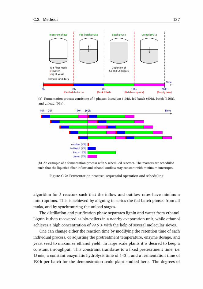
C.2. Methods 137
(a) Fermentation process consisting of 4 phases: inoculum (10 h), fed-batch (60 h), batch (120 h),and unload (70 h).
(b) An example of a fermentation process with 5 scheduled reactors. The reactors are scheduledsuch that the liquefied fiber inflow and ethanol outflow stay constant with minimum interrupts.
Figure C.2: Fermentation process: sequential operation and scheduling.
algorithm for 5 reactors such that the inflow and outflow rates have minimum
interruptions. This is achieved by aligning in series the fed-batch phases from all
tanks, and by synchronizing the unload stages.
The distillation and purification phase separates lignin and water from ethanol.
Lignin is then recovered as bio-pellets in a nearby evaporation unit, while ethanol
achieves a high concentration of 99.5 % with the help of several molecular sieves.
One can change either the reaction time by modifying the retention time of each
individual process, or adjusting the pretreatment temperature, enzyme dosage, and
yeast seed to maximize ethanol yield. In large scale plants it is desired to keep a
constant throughput. This constraint translates to a fixed pretreatment time, i.e.
15 min, a constant enzymatic hydrolysis time of 140 h, and a fermentation time of
190 h per batch for the demonstration scale plant studied here. The degrees of
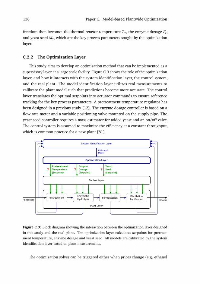
138 Paper C. Model-based Plantwide Optimization
freedom then become: the thermal reactor temperature Ttr, the enzyme dosage Fe,
and yeast seed My, which are the key process parameters sought by the optimization
layer.
C.2.2 The Optimization Layer
This study aims to develop an optimization method that can be implemented as a
supervisory layer at a large scale facility. Figure C.3 shows the role of the optimization
layer, and how it interacts with the system identification layer, the control system,
and the real plant. The model identification layer utilizes real measurements to
calibrate the plant model such that predictions become more accurate. The control
layer translates the optimal setpoints into actuator commands to ensure reference
tracking for the key process parameters. A pretreatment temperature regulator has
been designed in a previous study [12]. The enzyme dosage controller is based on a
flow rate meter and a variable positioning valve mounted on the supply pipe. The
yeast seed controller requires a mass estimator for added yeast and an on/off valve.
The control system is assumed to maximize the efficiency at a constant throughput,
which is common practice for a new plant [81].
Figure C.3: Block diagram showing the interaction between the optimization layer designed
in this study and the real plant. The optimization layer calculates setpoints for pretreat-
ment temperature, enzyme dosage and yeast seed. All models are calibrated by the system
identification layer based on plant measurements.
The optimization solver can be triggered either when prices change (e.g. ethanol

C.2. Methods 139
price increases, enzymes price decreases, yeast can be grown at a lower price
etc.), or when disturbances occur in the process (e.g. changes in feedstock content
due to biomass composition variety, or biomass type change). The solution of the
optimization problem provides setpoints for the pretreatment temperature, enzyme
dosage, and yeast seed. The system constraints are formulated based on validated
large scale models for: hydrothermal pretreatment with steam [5], enzymatic
hydrolysis [6], and C5 and C6 co-fermentation [74]. The optimizer searches for the
best nominal operational point by evaluating different scenarios with the help of
an integrated biorefinery simulator that embeds all these models. The optimization
problem has the following generic formulation [82]:
maxu
c(x,u)
subject to f (x,u) = 0g(x,u)≤ 0
(C.1)
where u is a vector of the decision variables or degrees of freedom, x represents the
process variables, and c(x,u) is the objective function. f (x,u) = 0 and g(x,u)≤ 0 are
equality and inequality constraints as functions of process and decision variables.
Optimization problem (C.1) is solved in a scientific software that has a solver for
finding the minimum of a constrained nonlinear multivariable function.
C.2.3 Mathematical Models
The optimization layer uses a dynamic biorefinery simulator to calculate the
stabilized or steady-state process outputs for pretreatment and enzymatic hydrolysis.
The mathematical models are complex and nonlinear. Finding an analytical solution
for steady-states is not trivial. An alternative is to run a sufficient long simulation
until all outputs are stabilized. The fermentation model is a batch process and the
outputs are collected after running a dynamic simulation for 190 h, i.e. the end of
the batch phase, which is a fixed amount of time due to a constant throughput. The
pretreatment and enzymatic hydrolysis models have already been published in [5]
and [6], and a summary of all equations is given in the supplementary material. The
fermentation model is detailed next.
C.2.3.1 C5 and C6 Co-Fermentation Model
The fermentation tank is modeled as a continuous stirred tank reactor (CSTR)
with reaction kinetics derived from [74]. Since it can take 70 h for filling the tank, it
is important to track the total mass change in time:
dM f
dt= Fin f −Fout f (C.2)

140 Paper C. Model-based Plantwide Optimization
where M f is the fermenter hold-up in kg, and Fin f and Fout f are the mass inflow and
outflow rates in kgs−1.
Component composition is tracked with the following equation for variable
hold-up:d(C f M f )
dt= Fin f Cin f −Fout f C f +R f M f (C.3)
where C f is the composition vector in gkg−1, Cin f is the inflow composition of
liquefied fibers coming from the enzymatic hydrolysis process, and R f is the reaction
rate vector in g/(kgs).Substituting Equation (C.2) into (C.3) yields:
dC f
dt=
1M f
[Fin f
(Cin f −C f
)]+R f (C.4)
The reaction rates are calculated using standard global black box model to
represent fermentation activity [119]:
• Glucose uptake:
RG =−qGI (C.5)
where RG is the glucose uptake rate, and equals the glucose consumption rate
with inhibition qGI , which is calculated as follows:
qGI =1
YEthG
qEthGI(C.6)
YEthG is the yield parameter for ethanol production from glucose. qEthGIrepre-
sents ethanol production rate from glucose with inhibition:
qEthGI= qEthG · IEthG · IFG · IAG · IHMFG (C.7)
qEthG is ethanol production from glucose only with substrate inhibition, while
IEthG , IFG , IAG , and IHMFG are inhibitory terms for ethanol (product inhibition),
furfural, acetate, and 5-HMF respectively. qEthG is modeled as in [120] with
pH dependency extension:
qEthG = qMaxG(pH) ·CCellCG
KSPG +CG +CG
2
KIPG
(C.8)
where CG and CCell are glucose and cell biomass concentrations, and KSPG and
KIPG are glucose self-inhibition terms.

C.2. Methods 141
The pH dependency is built empirically to resemble a bell with qMaxG as peak:
qMaxG(pH) = qMaxG
K0G(1+
10pH
K1G
+K2G
10pH
) (C.9)
where K0G , K1G , and K2G parametrize the shape of the bell.
Ethanol inhibition on glucose uptake or product inhibition has been defined in
[120]:
IEthG = 1−(
CEth
PMPG
)γG
(C.10)
with PMPG and γG as parameters. CEth is the concentration of ethanol.
Furfural, acetate and 5-HMF inhibition are modeled as below:
IiG =KIiG
KIiG+Ci
(C.11)
where IiG is the inhibition from component i, KIiGis the inhibitory constant,
and Ci is the concentration. Index i can be {F , Ac, HMF} signifying furfural,
acetate, or 5-HMF.
• Xylose uptake follows the same equation structure as glucose uptake but with
different parameter values:
RX =−qXI (C.12)
Xylose consumption with inhibition is calculated based on ethanol production
from xylose qEthXIwith inhibition, and yield parameter YEthX :
qXI =1
YEthX
qEthXI(C.13)
Ethanol production from xylose comprises inhibition terms from product IEthX ,
furfural IFX , acetate IAcX , and 5-HMF IHMFX :
qEthXI= qEthX · IEthX · IFX · IAcX · IHMFX (C.14)
qEthX shows ethanol production with substrate inhibition modeled as in [120]
with pH dependency extension:
qEthX = qMaxX (pH) ·CCellCX
KSPX +CX +CX
2
KIPX
(C.15)
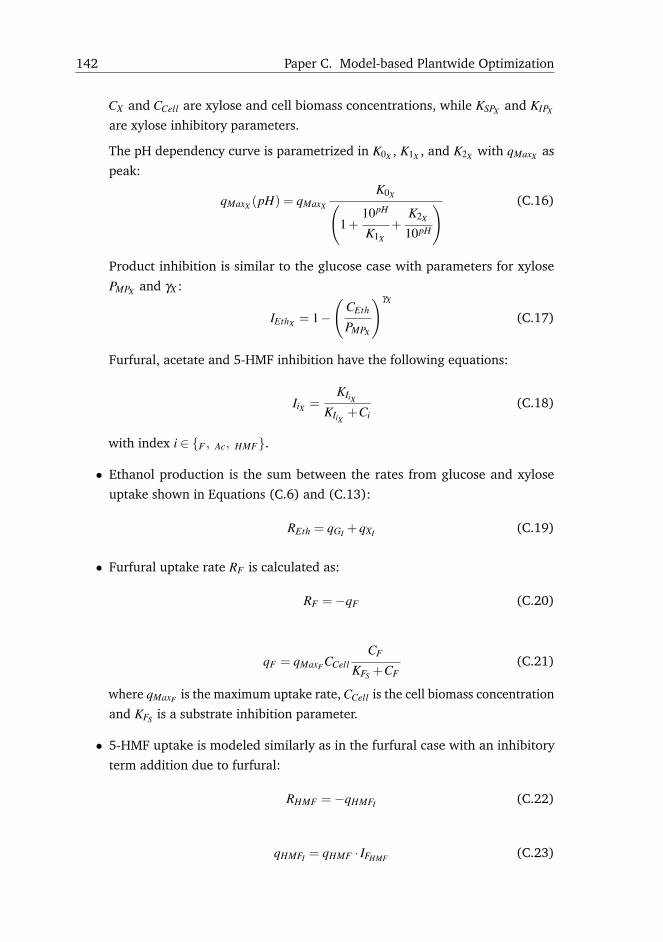
142 Paper C. Model-based Plantwide Optimization
CX and CCell are xylose and cell biomass concentrations, while KSPX and KIPX
are xylose inhibitory parameters.
The pH dependency curve is parametrized in K0X , K1X , and K2X with qMaxX as
peak:
qMaxX (pH) = qMaxX
K0X(1+
10pH
K1X
+K2X
10pH
) (C.16)
Product inhibition is similar to the glucose case with parameters for xylose
PMPX and γX :
IEthX = 1−(
CEth
PMPX
)γX
(C.17)
Furfural, acetate and 5-HMF inhibition have the following equations:
IiX =KIiX
KIiX+Ci
(C.18)
with index i ∈ {F , Ac, HMF}.
• Ethanol production is the sum between the rates from glucose and xylose
uptake shown in Equations (C.6) and (C.13):
REth = qGI +qXI (C.19)
• Furfural uptake rate RF is calculated as:
RF =−qF (C.20)
qF = qMaxF CCellCF
KFS +CF(C.21)
where qMaxF is the maximum uptake rate, CCell is the cell biomass concentration
and KFS is a substrate inhibition parameter.
• 5-HMF uptake is modeled similarly as in the furfural case with an inhibitory
term addition due to furfural:
RHMF =−qHMFI (C.22)
qHMFI = qHMF · IFHMF (C.23)
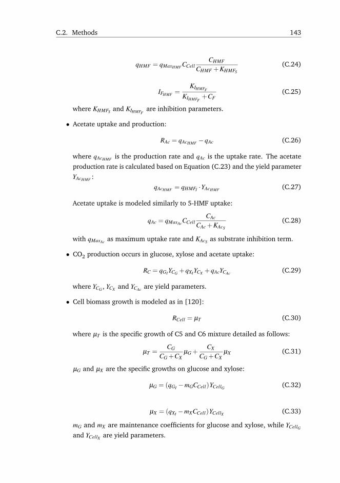
C.2. Methods 143
qHMF = qMaxHMF CCellCHMF
CHMF +KHMFS
(C.24)
IFHMF =KIHMFF
KIHMFF+CF
(C.25)
where KHMFS and KIHMFFare inhibition parameters.
• Acetate uptake and production:
RAc = qAcHMF −qAc (C.26)
where qAcHMF is the production rate and qAc is the uptake rate. The acetate
production rate is calculated based on Equation (C.23) and the yield parameter
YAcHMF :
qAcHMF = qHMFI ·YAcHMF (C.27)
Acetate uptake is modeled similarly to 5-HMF uptake:
qAc = qMaxAcCCellCAc
CAc +KAcS
(C.28)
with qMaxAc as maximum uptake rate and KAcS as substrate inhibition term.
• CO2 production occurs in glucose, xylose and acetate uptake:
RC = qGIYCG +qXIYCX +qAcYCAc (C.29)
where YCG , YCX and YCAc are yield parameters.
• Cell biomass growth is modeled as in [120]:
RCell = µT (C.30)
where µT is the specific growth of C5 and C6 mixture detailed as follows:
µT =CG
CG +CXµG +
CX
CG +CXµX (C.31)
µG and µX are the specific growths on glucose and xylose:
µG = (qGI −mGCCell)YCellG (C.32)
µX = (qXI −mXCCell)YCellX (C.33)
mG and mX are maintenance coefficients for glucose and xylose, while YCellG
and YCellX are yield parameters.
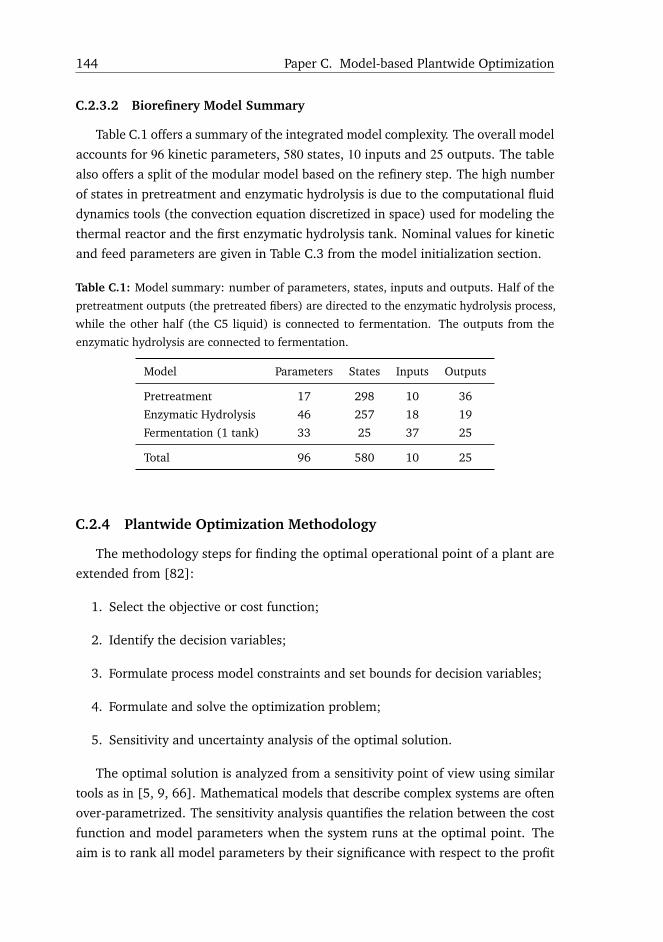
144 Paper C. Model-based Plantwide Optimization
C.2.3.2 Biorefinery Model Summary
Table C.1 offers a summary of the integrated model complexity. The overall model
accounts for 96 kinetic parameters, 580 states, 10 inputs and 25 outputs. The table
also offers a split of the modular model based on the refinery step. The high number
of states in pretreatment and enzymatic hydrolysis is due to the computational fluid
dynamics tools (the convection equation discretized in space) used for modeling the
thermal reactor and the first enzymatic hydrolysis tank. Nominal values for kinetic
and feed parameters are given in Table C.3 from the model initialization section.
Table C.1: Model summary: number of parameters, states, inputs and outputs. Half of the
pretreatment outputs (the pretreated fibers) are directed to the enzymatic hydrolysis process,
while the other half (the C5 liquid) is connected to fermentation. The outputs from the
enzymatic hydrolysis are connected to fermentation.
Model Parameters States Inputs Outputs
Pretreatment 17 298 10 36
Enzymatic Hydrolysis 46 257 18 19
Fermentation (1 tank) 33 25 37 25
Total 96 580 10 25
C.2.4 Plantwide Optimization Methodology
The methodology steps for finding the optimal operational point of a plant are
extended from [82]:
1. Select the objective or cost function;
2. Identify the decision variables;
3. Formulate process model constraints and set bounds for decision variables;
4. Formulate and solve the optimization problem;
5. Sensitivity and uncertainty analysis of the optimal solution.
The optimal solution is analyzed from a sensitivity point of view using similar
tools as in [5, 9, 66]. Mathematical models that describe complex systems are often
over-parametrized. The sensitivity analysis quantifies the relation between the cost
function and model parameters when the system runs at the optimal point. The
aim is to rank all model parameters by their significance with respect to the profit
C.3. Results and Discussion 145
value at the nominal operational point. Also a subset of relevant parameters can be
extracted for calculating the uncertainty bounds.
A measure of sensitivity suitable for steady-state signals is [8, 64]:
δk =∂ck
∂θk
θk
cssk
(C.34)
where ∂ck/∂θk is the variation in profit with respect to a model parameter, and is
calculated based on finite differences. θk is the kth parameter, and cssk is the profit or
the value of the cost function in steady-state. All model parameters are sorted in
descending order with respect to δk, and a subset is created with all parameters that
have δk above a threshold. The reduced subset of model parameters is then used in
the uncertainty analysis.
The propagation of uncertainty is analyzed with a Monte Carlo procedure as
described in [9]:
1. Define input uncertainty;
2. Parameter sampling;
3. Monte Carlo simulations;
4. Output uncertainty.
The input uncertainty is defined with standard deviations and correlation matri-
ces obtained from previous studies. Dealing with many parameters implies a large
number of combinations of parameter values with high correlation between them.
In order to reduce the number of parameter samples, a Latin Hypercube Sampling
(LHS) technique with correlation control is utilized [65]. LHS generates less samples
of parameters but still statistically plausible with the help of a distribution function,
standard deviation, and correlation matrix. For each set of samples, a simulation
is then run and the output is collected. After all Monte-Carlo simulations are per-
formed, enough output information is obtained to statistically compute the median
and the 5th-95th percentile confidence interval.
C.3 Results and Discussion
This section starts with model initialization where the values of both model
and feed parameters are given in tabular format. The solution of the optimization
problem is then found and discussed. The sensitivity analysis with respect to model
kinetic parameters follows. A parameter subset is then identified, which is used in
Monte Carlo simulations for quantifying the uncertainty of the optimal solution. The
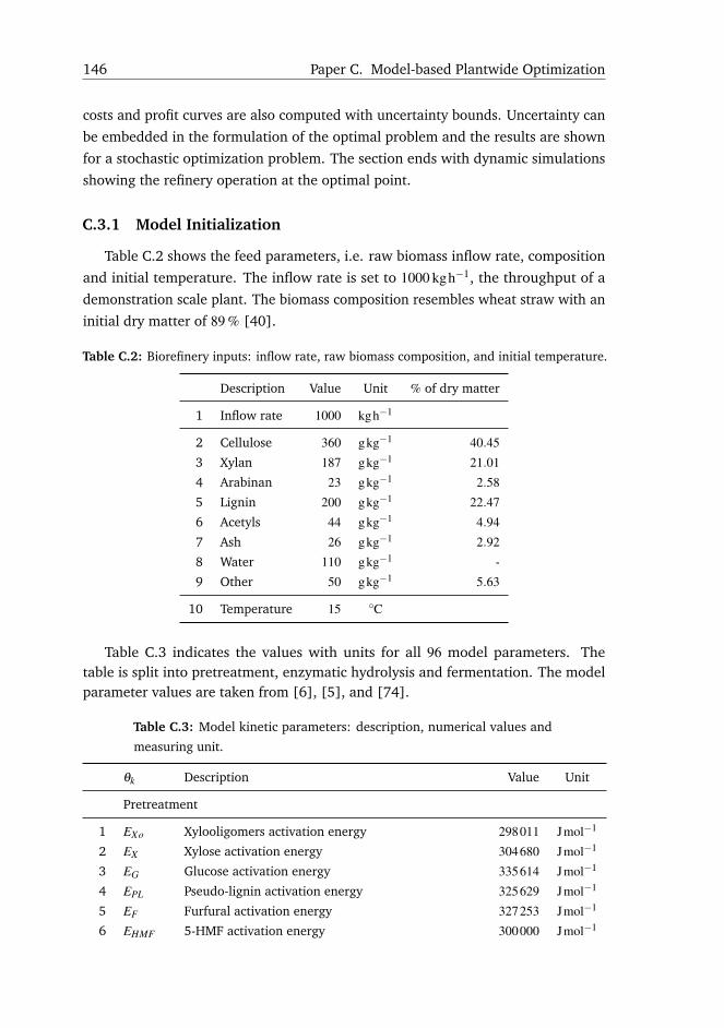
146 Paper C. Model-based Plantwide Optimization
costs and profit curves are also computed with uncertainty bounds. Uncertainty can
be embedded in the formulation of the optimal problem and the results are shown
for a stochastic optimization problem. The section ends with dynamic simulations
showing the refinery operation at the optimal point.
C.3.1 Model Initialization
Table C.2 shows the feed parameters, i.e. raw biomass inflow rate, composition
and initial temperature. The inflow rate is set to 1000 kgh−1, the throughput of a
demonstration scale plant. The biomass composition resembles wheat straw with an
initial dry matter of 89 % [40].
Table C.2: Biorefinery inputs: inflow rate, raw biomass composition, and initial temperature.
Description Value Unit % of dry matter
1 Inflow rate 1000 kgh−1
2 Cellulose 360 gkg−1 40.45
3 Xylan 187 gkg−1 21.01
4 Arabinan 23 gkg−1 2.58
5 Lignin 200 gkg−1 22.47
6 Acetyls 44 gkg−1 4.94
7 Ash 26 gkg−1 2.92
8 Water 110 gkg−1 -
9 Other 50 gkg−1 5.63
10 Temperature 15 ◦C
Table C.3 indicates the values with units for all 96 model parameters. Thetable is split into pretreatment, enzymatic hydrolysis and fermentation. The modelparameter values are taken from [6], [5], and [74].
Table C.3: Model kinetic parameters: description, numerical values and
measuring unit.
θk Description Value Unit
Pretreatment
1 EXo Xylooligomers activation energy 298011 Jmol−1
2 EX Xylose activation energy 304680 Jmol−1
3 EG Glucose activation energy 335614 Jmol−1
4 EPL Pseudo-lignin activation energy 325629 Jmol−1
5 EF Furfural activation energy 327253 Jmol−1
6 EHMF 5-HMF activation energy 300000 Jmol−1
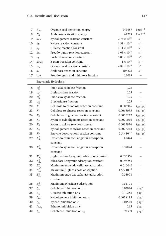
C.3. Results and Discussion 147
7 EAc Organic acid activation energy 242687 Jmol−1
8 EA Arabinose activation energy 61229 Jmol−1
9 kXo Xylooligomers reaction constant 2.78×1031 s−1
10 kX Xylose reaction constant 1.31×1034 s−1
11 kG Glucose reaction constant 1.11×1035 s−1
12 kPL Pseudo-lignin reaction constant 1.03×1033 s−1
13 kF Furfural reaction constant 5.09×1033 s−1
14 kHMF 5-HMF reaction constant 1×1031 s−1
15 kAc Organic acid reaction constant 4.88×1024 s−1
16 kA Arabinose reaction constant 106225 s−1
17 αPL Pseudo-lignin and inhibitors fraction 0.1019 −
Enzymatic Hydrolysis
18 αEC Endo-exo cellulase fraction 0.25 −
19 αGC β -glucosidase fraction 0.25 −
20 αEX Endo-exo xylanase fraction 0.25 −
21 αGX β -xylosidase fraction 0.25 −
22 K1 Cellulose to cellobiose reaction constant 0.005916 kg/(gs)
23 K2 Cellulose to glucose reaction constant 0.0065075 kg/(gs)
24 K3 Cellobiose to glucose reaction constant 0.0055227 kg/(gs)
25 K4 Xylan to xylooligomers reaction constant 0.0020026 kg/(gs)
26 K5 Xylan to xylose reaction constant 0.0033936 kg/(gs)
27 K6 Xylooligomers to xylose reaction constant 0.0028228 kg/(gs)
28 K7 Enzyme deactivation reaction constant 2.5×10⁻⁷ kg/(gs)
29 KEAC
Exo-endo cellulase Langmuir adsorption
constant
1.0444 −
30 KEAX
Exo-endo xylanase Langmuir adsorption
constant
0.37844 −
31 KGAC
β -glucosidase Langmuir adsorption constant 0.056976 −32 KX
AXXilosidase Langmuir adsorption constant 0.093253 −
33 EEMC
Maximum exo-endo cellulase adsorption 0.016042 −34 EG
MCMaximum β -glucosidase adsorption 1.5×10⁻⁵ −
35 EEMX
Maximum endo-exo xylanase adsorption
constant
0.38978 −
36 EXMX
Maximum xylosidase adsorption 0.51178 −37 IC1 Cellobiose inhibition on r1 0.02014 gkg−1
38 IG1 Glucose inhibition on r1 0.10255 gkg−1
39 IXo1 Xylooligomers inhibition on r1 0.0078145 gkg−1
40 IX1 Xylose inhibition on r1 0.01503 gkg−1
41 IEth1 Ethanol inhibition on r1 0.15 gkg−1
42 IC2 Cellobiose inhibition on r2 69.539 gkg−1
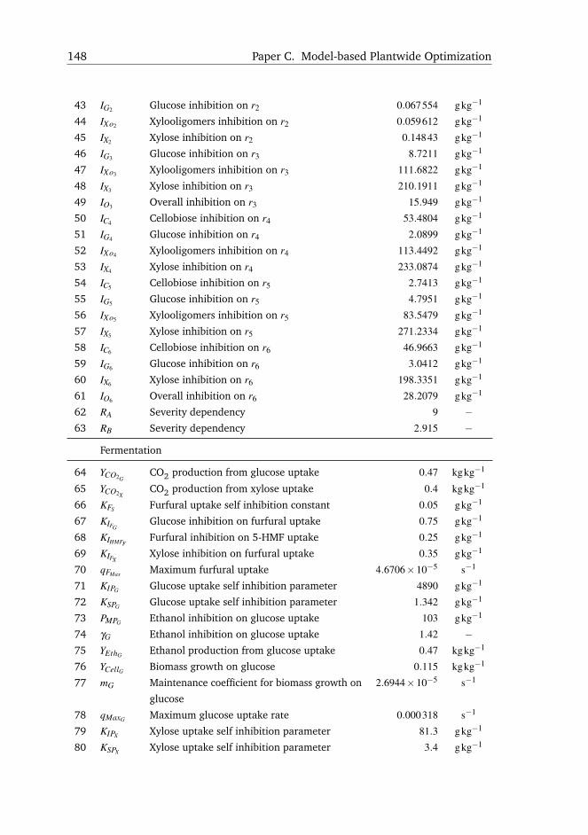
148 Paper C. Model-based Plantwide Optimization
43 IG2 Glucose inhibition on r2 0.067554 gkg−1
44 IXo2 Xylooligomers inhibition on r2 0.059612 gkg−1
45 IX2 Xylose inhibition on r2 0.14843 gkg−1
46 IG3 Glucose inhibition on r3 8.7211 gkg−1
47 IXo3 Xylooligomers inhibition on r3 111.6822 gkg−1
48 IX3 Xylose inhibition on r3 210.1911 gkg−1
49 IO3 Overall inhibition on r3 15.949 gkg−1
50 IC4 Cellobiose inhibition on r4 53.4804 gkg−1
51 IG4 Glucose inhibition on r4 2.0899 gkg−1
52 IXo4 Xylooligomers inhibition on r4 113.4492 gkg−1
53 IX4 Xylose inhibition on r4 233.0874 gkg−1
54 IC5 Cellobiose inhibition on r5 2.7413 gkg−1
55 IG5 Glucose inhibition on r5 4.7951 gkg−1
56 IXo5 Xylooligomers inhibition on r5 83.5479 gkg−1
57 IX5 Xylose inhibition on r5 271.2334 gkg−1
58 IC6 Cellobiose inhibition on r6 46.9663 gkg−1
59 IG6 Glucose inhibition on r6 3.0412 gkg−1
60 IX6 Xylose inhibition on r6 198.3351 gkg−1
61 IO6 Overall inhibition on r6 28.2079 gkg−1
62 RA Severity dependency 9 −63 RB Severity dependency 2.915 −
Fermentation
64 YCO2GCO2 production from glucose uptake 0.47 kgkg−1
65 YCO2XCO2 production from xylose uptake 0.4 kgkg−1
66 KFS Furfural uptake self inhibition constant 0.05 gkg−1
67 KIFGGlucose inhibition on furfural uptake 0.75 gkg−1
68 KIHMFFFurfural inhibition on 5-HMF uptake 0.25 gkg−1
69 KIFXXylose inhibition on furfural uptake 0.35 gkg−1
70 qFMax Maximum furfural uptake 4.6706×10⁻⁵ s−1
71 KIPG Glucose uptake self inhibition parameter 4890 gkg−1
72 KSPG Glucose uptake self inhibition parameter 1.342 gkg−1
73 PMPG Ethanol inhibition on glucose uptake 103 gkg−1
74 γG Ethanol inhibition on glucose uptake 1.42 −75 YEthG Ethanol production from glucose uptake 0.47 kgkg−1
76 YCellG Biomass growth on glucose 0.115 kgkg−1
77 mG Maintenance coefficient for biomass growth on
glucose
2.6944×10⁻⁵ s−1
78 qMaxG Maximum glucose uptake rate 0.000318 s−1
79 KIPX Xylose uptake self inhibition parameter 81.3 gkg−1
80 KSPX Xylose uptake self inhibition parameter 3.4 gkg−1
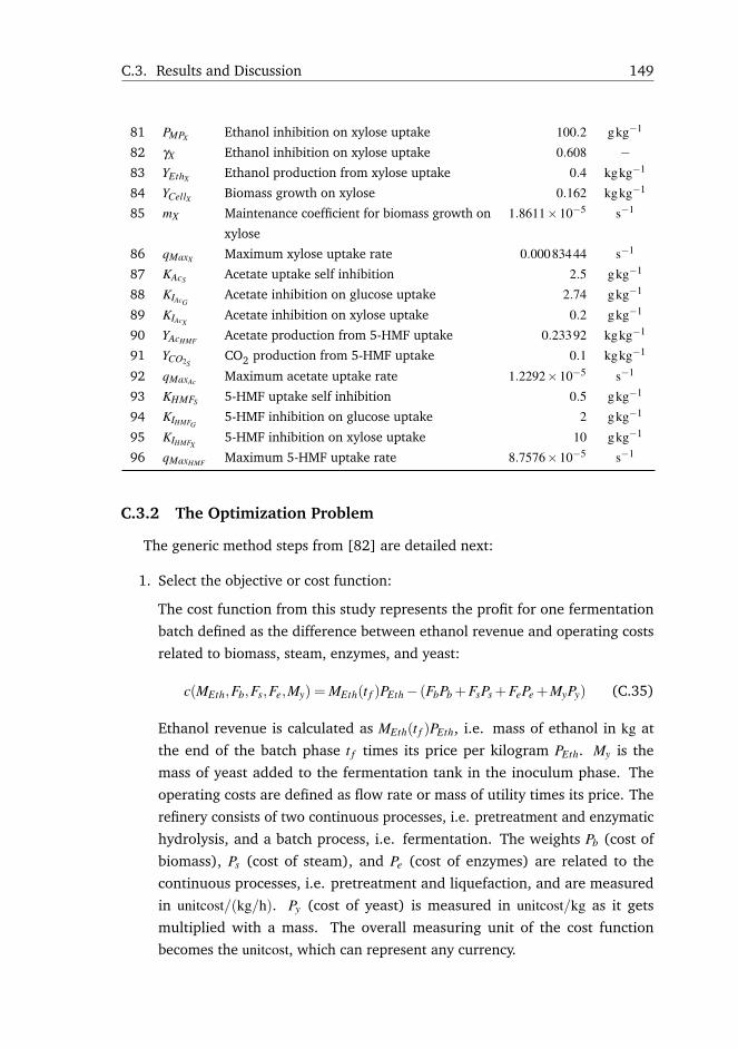
C.3. Results and Discussion 149
81 PMPX Ethanol inhibition on xylose uptake 100.2 gkg−1
82 γX Ethanol inhibition on xylose uptake 0.608 −83 YEthX Ethanol production from xylose uptake 0.4 kgkg−1
84 YCellX Biomass growth on xylose 0.162 kgkg−1
85 mX Maintenance coefficient for biomass growth on
xylose
1.8611×10⁻⁵ s−1
86 qMaxX Maximum xylose uptake rate 0.00083444 s−1
87 KAcS Acetate uptake self inhibition 2.5 gkg−1
88 KIAcGAcetate inhibition on glucose uptake 2.74 gkg−1
89 KIAcXAcetate inhibition on xylose uptake 0.2 gkg−1
90 YAcHMF Acetate production from 5-HMF uptake 0.23392 kgkg−1
91 YCO2SCO2 production from 5-HMF uptake 0.1 kgkg−1
92 qMaxAc Maximum acetate uptake rate 1.2292×10⁻⁵ s−1
93 KHMFS 5-HMF uptake self inhibition 0.5 gkg−1
94 KIHMFG5-HMF inhibition on glucose uptake 2 gkg−1
95 KIHMFX5-HMF inhibition on xylose uptake 10 gkg−1
96 qMaxHMF Maximum 5-HMF uptake rate 8.7576×10⁻⁵ s−1
C.3.2 The Optimization Problem
The generic method steps from [82] are detailed next:
1. Select the objective or cost function:
The cost function from this study represents the profit for one fermentation
batch defined as the difference between ethanol revenue and operating costs
related to biomass, steam, enzymes, and yeast:
c(MEth,Fb,Fs,Fe,My) = MEth(t f )PEth− (FbPb +FsPs +FePe +MyPy) (C.35)
Ethanol revenue is calculated as MEth(t f )PEth, i.e. mass of ethanol in kg at
the end of the batch phase t f times its price per kilogram PEth. My is the
mass of yeast added to the fermentation tank in the inoculum phase. The
operating costs are defined as flow rate or mass of utility times its price. The
refinery consists of two continuous processes, i.e. pretreatment and enzymatic
hydrolysis, and a batch process, i.e. fermentation. The weights Pb (cost of
biomass), Ps (cost of steam), and Pe (cost of enzymes) are related to the
continuous processes, i.e. pretreatment and liquefaction, and are measured
in unitcost/(kg/h). Py (cost of yeast) is measured in unitcost/kg as it gets
multiplied with a mass. The overall measuring unit of the cost function
becomes the unitcost, which can represent any currency.
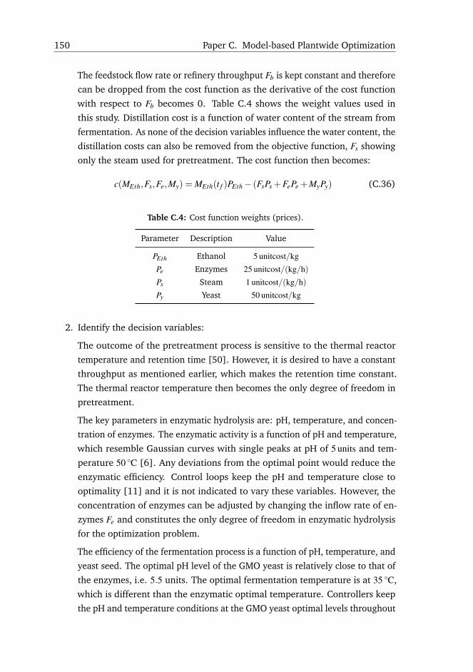
150 Paper C. Model-based Plantwide Optimization
The feedstock flow rate or refinery throughput Fb is kept constant and therefore
can be dropped from the cost function as the derivative of the cost function
with respect to Fb becomes 0. Table C.4 shows the weight values used in
this study. Distillation cost is a function of water content of the stream from
fermentation. As none of the decision variables influence the water content, the
distillation costs can also be removed from the objective function, Fs showing
only the steam used for pretreatment. The cost function then becomes:
c(MEth,Fs,Fe,My) = MEth(t f )PEth− (FsPs +FePe +MyPy) (C.36)
Table C.4: Cost function weights (prices).
Parameter Description Value
PEth Ethanol 5 unitcost/kg
Pe Enzymes 25 unitcost/(kg/h)
Ps Steam 1 unitcost/(kg/h)
Py Yeast 50 unitcost/kg
2. Identify the decision variables:
The outcome of the pretreatment process is sensitive to the thermal reactor
temperature and retention time [50]. However, it is desired to have a constant
throughput as mentioned earlier, which makes the retention time constant.
The thermal reactor temperature then becomes the only degree of freedom in
pretreatment.
The key parameters in enzymatic hydrolysis are: pH, temperature, and concen-
tration of enzymes. The enzymatic activity is a function of pH and temperature,
which resemble Gaussian curves with single peaks at pH of 5 units and tem-
perature 50 ◦C [6]. Any deviations from the optimal point would reduce the
enzymatic efficiency. Control loops keep the pH and temperature close to
optimality [11] and it is not indicated to vary these variables. However, the
concentration of enzymes can be adjusted by changing the inflow rate of en-
zymes Fe and constitutes the only degree of freedom in enzymatic hydrolysis
for the optimization problem.
The efficiency of the fermentation process is a function of pH, temperature, and
yeast seed. The optimal pH level of the GMO yeast is relatively close to that of
the enzymes, i.e. 5.5 units. The optimal fermentation temperature is at 35 ◦C,
which is different than the enzymatic optimal temperature. Controllers keep
the pH and temperature conditions at the GMO yeast optimal levels throughout
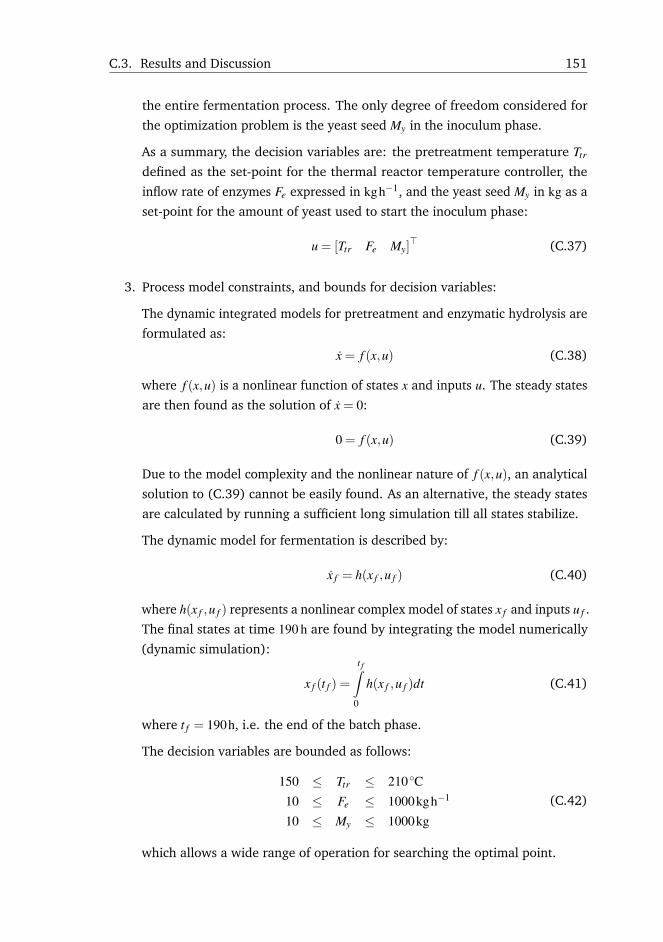
C.3. Results and Discussion 151
the entire fermentation process. The only degree of freedom considered for
the optimization problem is the yeast seed My in the inoculum phase.
As a summary, the decision variables are: the pretreatment temperature Ttr
defined as the set-point for the thermal reactor temperature controller, the
inflow rate of enzymes Fe expressed in kgh−1, and the yeast seed My in kg as a
set-point for the amount of yeast used to start the inoculum phase:
u = [Ttr Fe My]> (C.37)
3. Process model constraints, and bounds for decision variables:
The dynamic integrated models for pretreatment and enzymatic hydrolysis are
formulated as:
x = f (x,u) (C.38)
where f (x,u) is a nonlinear function of states x and inputs u. The steady states
are then found as the solution of x = 0:
0 = f (x,u) (C.39)
Due to the model complexity and the nonlinear nature of f (x,u), an analytical
solution to (C.39) cannot be easily found. As an alternative, the steady states
are calculated by running a sufficient long simulation till all states stabilize.
The dynamic model for fermentation is described by:
x f = h(x f ,u f ) (C.40)
where h(x f ,u f ) represents a nonlinear complex model of states x f and inputs u f .
The final states at time 190 h are found by integrating the model numerically
(dynamic simulation):
x f (t f ) =
t f∫0
h(x f ,u f )dt (C.41)
where t f = 190h, i.e. the end of the batch phase.
The decision variables are bounded as follows:
150 ≤ Ttr ≤ 210 ◦C10 ≤ Fe ≤ 1000kgh−1
10 ≤ My ≤ 1000kg
(C.42)
which allows a wide range of operation for searching the optimal point.
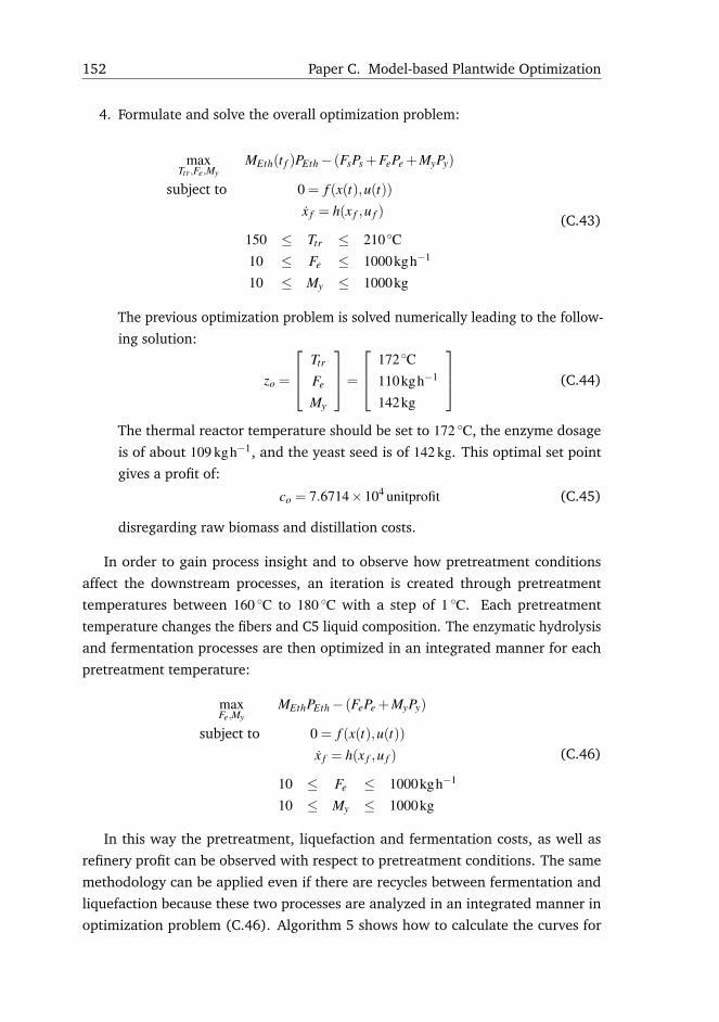
152 Paper C. Model-based Plantwide Optimization
4. Formulate and solve the overall optimization problem:
maxTtr ,Fe,My
MEth(t f )PEth− (FsPs +FePe +MyPy)
subject to 0 = f (x(t),u(t))
x f = h(x f ,u f )
150 ≤ Ttr ≤ 210 ◦C10 ≤ Fe ≤ 1000kgh−1
10 ≤ My ≤ 1000kg
(C.43)
The previous optimization problem is solved numerically leading to the follow-
ing solution:
zo =
Ttr
Fe
My
=
172 ◦C110kgh−1
142kg
(C.44)
The thermal reactor temperature should be set to 172 ◦C, the enzyme dosage
is of about 109 kgh−1, and the yeast seed is of 142 kg. This optimal set point
gives a profit of:
co = 7.6714×10⁴ unitprofit (C.45)
disregarding raw biomass and distillation costs.
In order to gain process insight and to observe how pretreatment conditions
affect the downstream processes, an iteration is created through pretreatment
temperatures between 160 ◦C to 180 ◦C with a step of 1 ◦C. Each pretreatment
temperature changes the fibers and C5 liquid composition. The enzymatic hydrolysis
and fermentation processes are then optimized in an integrated manner for each
pretreatment temperature:
maxFe,My
MEthPEth− (FePe +MyPy)
subject to 0 = f (x(t),u(t))
x f = h(x f ,u f )
10 ≤ Fe ≤ 1000kgh−1
10 ≤ My ≤ 1000kg
(C.46)
In this way the pretreatment, liquefaction and fermentation costs, as well as
refinery profit can be observed with respect to pretreatment conditions. The same
methodology can be applied even if there are recycles between fermentation and
liquefaction because these two processes are analyzed in an integrated manner in
optimization problem (C.46). Algorithm 5 shows how to calculate the curves for
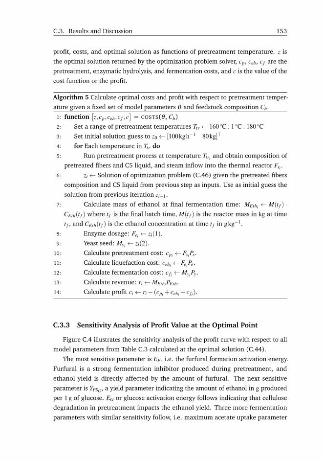
C.3. Results and Discussion 153
profit, costs, and optimal solution as functions of pretreatment temperature. z is
the optimal solution returned by the optimization problem solver, cp, ceh, c f are the
pretreatment, enzymatic hydrolysis, and fermentation costs, and c is the value of the
cost function or the profit.
Algorithm 5 Calculate optimal costs and profit with respect to pretreatment temper-
ature given a fixed set of model parameters θ and feedstock composition Cb.
1: function[z,cp,ceh,c f ,c
]= COSTS(θ , Cb)
2: Set a range of pretreatment temperatures Ttr← 160 ◦C : 1 ◦C : 180 ◦C3: Set initial solution guess to z0← [100kgh−1 80kg]>
4: for Each temperature in Ttr do
5: Run pretreatment process at temperature Ttri and obtain composition of
pretreated fibers and C5 liquid, and steam inflow into the thermal reactor Fsi .
6: zi← Solution of optimization problem (C.46) given the pretreated fibers
composition and C5 liquid from previous step as inputs. Use as initial guess the
solution from previous iteration zi−1.
7: Calculate mass of ethanol at final fermentation time: MEthi ← M(t f ) ·CEth(t f ) where t f is the final batch time, M(t f ) is the reactor mass in kg at time
t f , and CEth(t f ) is the ethanol concentration at time t f in gkg−1.
8: Enzyme dosage: Fei ← zi(1).9: Yeast seed: Myi ← zi(2).
10: Calculate pretreatment cost: cpi ← FsiPs.
11: Calculate liquefaction cost: cehi ← FeiPe.
12: Calculate fermentation cost: c fi ←MyiPy.
13: Calculate revenue: ri←MEthiPEth.
14: Calculate profit ci← ri− (cpi + cehi + c fi).
C.3.3 Sensitivity Analysis of Profit Value at the Optimal Point
Figure C.4 illustrates the sensitivity analysis of the profit curve with respect to all
model parameters from Table C.3 calculated at the optimal solution (C.44).
The most sensitive parameter is EF , i.e. the furfural formation activation energy.
Furfural is a strong fermentation inhibitor produced during pretreatment, and
ethanol yield is directly affected by the amount of furfural. The next sensitive
parameter is YPSG , a yield parameter indicating the amount of ethanol in g produced
per 1 g of glucose. EG or glucose activation energy follows indicating that cellulose
degradation in pretreatment impacts the ethanol yield. Three more fermentation
parameters with similar sensitivity follow, i.e. maximum acetate uptake parameter
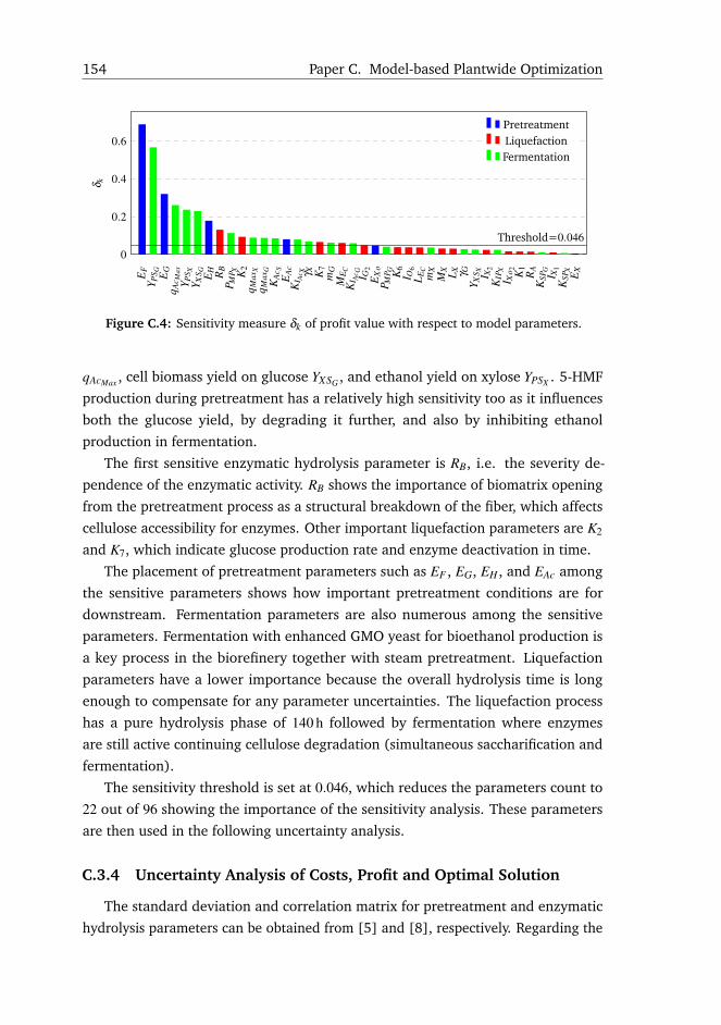
154 Paper C. Model-based Plantwide Optimization
EF
Y PS G EG
q Ac M
axY P
S XY X
S G EH RB
P MP X K
2q M
axX
q Max
GK
Ac S
EA
cK
I Ac X γ X K
7m
GM
E CK
I Ac G I G
2E
Xo
P MP G K
6I O
6L E
Cm
XM
X L X γ GY X
S X I X2
KIP
XI X
o 2 K1
RA
KSP
GI X
1K
SPX
EX
0
0.2
0.4
0.6
Threshold=0.046
δ k
PretreatmentLiquefactionFermentation
Figure C.4: Sensitivity measure δk of profit value with respect to model parameters.
qAcMax , cell biomass yield on glucose YXSG , and ethanol yield on xylose YPSX . 5-HMF
production during pretreatment has a relatively high sensitivity too as it influences
both the glucose yield, by degrading it further, and also by inhibiting ethanol
production in fermentation.
The first sensitive enzymatic hydrolysis parameter is RB, i.e. the severity de-
pendence of the enzymatic activity. RB shows the importance of biomatrix opening
from the pretreatment process as a structural breakdown of the fiber, which affects
cellulose accessibility for enzymes. Other important liquefaction parameters are K2
and K7, which indicate glucose production rate and enzyme deactivation in time.
The placement of pretreatment parameters such as EF , EG, EH , and EAc among
the sensitive parameters shows how important pretreatment conditions are for
downstream. Fermentation parameters are also numerous among the sensitive
parameters. Fermentation with enhanced GMO yeast for bioethanol production is
a key process in the biorefinery together with steam pretreatment. Liquefaction
parameters have a lower importance because the overall hydrolysis time is long
enough to compensate for any parameter uncertainties. The liquefaction process
has a pure hydrolysis phase of 140 h followed by fermentation where enzymes
are still active continuing cellulose degradation (simultaneous saccharification and
fermentation).
The sensitivity threshold is set at 0.046, which reduces the parameters count to
22 out of 96 showing the importance of the sensitivity analysis. These parameters
are then used in the following uncertainty analysis.
C.3.4 Uncertainty Analysis of Costs, Profit and Optimal Solution
The standard deviation and correlation matrix for pretreatment and enzymatic
hydrolysis parameters can be obtained from [5] and [8], respectively. Regarding the

C.3. Results and Discussion 155
fermentation model, there is no real data that could be used to obtain parameter
estimates. However, one can generate measurements through simulation, i.e. glu-
cose, xylose and ethanol levels, add measurement noise, and then run a parameter
estimation procedure for estimating the standard deviation and correlation matrix
for these parameters, which is done here in this study.
Latin Hypercube Sampling (LHS) with correlation control can then be performed
for all model parameters. Feedstock composition is sampled with uniform LHS
considering a 5 % variation in composition. N = 44 samples are extracted for model
and feed parameters. The Monte Carlo simulations are performed by running
Algorithm 5 for each set of parameters. The simulation outputs are collected, and
the 5th, 50th and 95th percentiles are then calculated for profit, costs, and optimal
solution.
The uncertainty analysis is carried separately for feed, and then for model
parameters in order to observe the contribution of each source of uncertainty. A
last analysis combines the samples of feed and model parameters to find the overall
effect of the uncertainty sources on the outputs.
The entire sensitivity and uncertainty analysis for combined model and feed
parameters is summarized in Algorithm 6. To run a separate model, and then feed
uncertainty analysis, the algorithm can be trivially modified either by keeping Cb or
θ constant in step 11.
Algorithm 6 Sensitivity and uncertainty analysis with combined model and feed
parameters.1: Initialize model parameters θ and feed composition Cb.
2: Optimal deterministic solution: [Ttr,Fe,My]← (C.43).
3: Sensitivity analysis of the cost function in [Ttr,Fe,My]: calculate δk as in equation
(C.34).
4: Rank all parameters with respect to δk.
5: Select a subset θR such that θR is above a threshold.
6: Set standard deviations and correlation matrices for θR.
7: θ ← LHS of θR with correlation control to generate N sets of model parameters.
8: Set bounds for feedstock composition.
9: Cb← Uniform LHS for feedstock composition to generate N sets of compositions.
10: for Each set of model and feed parameters do
11:[zi,cpi ,cehi ,c fi ,ci
]= COSTS(θi,Cbi)
12: Calculate the 5th, median and 95th percentile for profit, costs, and optimal
solution.
The results of the uncertainty analysis are displayed in Figure C.5 and commented
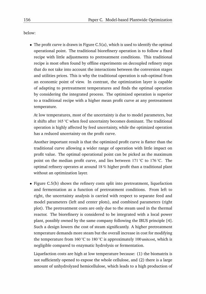
156 Paper C. Model-based Plantwide Optimization
below:
• The profit curve is drawn in Figure C.5(a), which is used to identify the optimal
operational point. The traditional biorefinery operation is to follow a fixed
recipe with little adjustments to pretreatment conditions. This traditional
recipe is most often found by offline experiments on decoupled refinery steps
that do not take into account the interactions between the conversion stages
and utilities prices. This is why the traditional operation is sub-optimal from
an economic point of view. In contrast, the optimization layer is capable
of adapting to pretreatment temperatures and finds the optimal operation
by considering the integrated process. The optimized operation is superior
to a traditional recipe with a higher mean profit curve at any pretreatment
temperature.
At low temperatures, most of the uncertainty is due to model parameters, but
it shifts after 165 ◦C when feed uncertainty becomes dominant. The traditional
operation is highly affected by feed uncertainty, while the optimized operation
has a reduced uncertainty on the profit curve.
Another important result is that the optimized profit curve is flatter than the
traditional curve allowing a wider range of operation with little impact on
profit value. The optimal operational point can be picked as the maximum
point on the median profit curve, and lies between 171 ◦C to 176 ◦C. The
optimal refinery operates at around 18 % higher profit than a traditional plant
without an optimization layer.
• Figure C.5(b) shows the refinery costs split into pretreatment, liquefaction
and fermentation as a function of pretreatment conditions. From left to
right, the uncertainty analysis is carried with respect to separate feed and
model parameters (left and center plots), and combined parameters (right
plot). The pretreatment costs are only due to the steam used in the thermal
reactor. The biorefinery is considered to be integrated with a local power
plant, possibly owned by the same company following the IBUS principle [4].
Such a design lowers the cost of steam significantly. A higher pretreatment
temperature demands more steam but the overall increase in cost for modifying
the temperature from 160 ◦C to 180 ◦C is approximately 100 unitcost, which is
negligible compared to enzymatic hydrolysis or fermentation.
Liquefaction costs are high at low temperature because: (1) the biomatrix is
not sufficiently opened to expose the whole cellulose, and (2) there is a large
amount of unhydrolyzed hemicellulose, which leads to a high production of
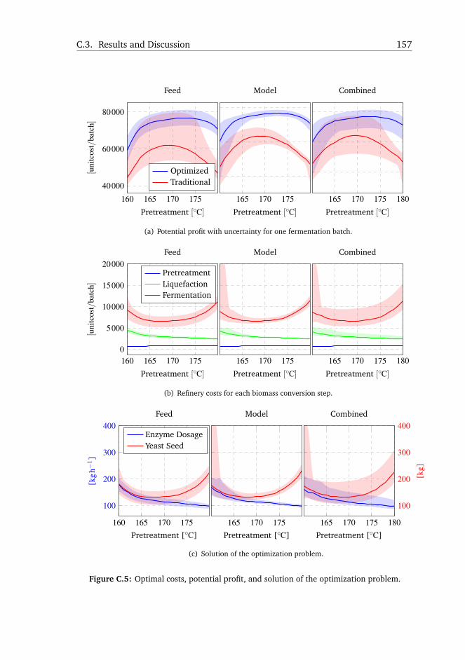
C.3. Results and Discussion 157
160 165 170 175
40000
60000
80000
Pretreatment [◦C]
[uni
tcos
t/ba
tch]
Feed
OptimizedTraditional
165 170 175
Pretreatment [◦C]
Model
165 170 175 180
Pretreatment [◦C]
Combined
(a) Potential profit with uncertainty for one fermentation batch.
160 165 170 1750
5000
10000
15000
20000
Pretreatment [◦C]
[uni
tcos
t/ba
tch]
Feed
PretreatmentLiquefactionFermentation
165 170 175
Pretreatment [◦C]
Model
165 170 175 180
Pretreatment [◦C]
Combined
(b) Refinery costs for each biomass conversion step.
160 165 170 175
100
200
300
400
Pretreatment [◦C]
[kg
h−1 ]
Feed
Enzyme DosageYeast Seed
165 170 175
Pretreatment [◦C]
Model
165 170 175 180
100
200
300
400
Pretreatment [◦C]
[kg]
Combined
(c) Solution of the optimization problem.
Figure C.5: Optimal costs, potential profit, and solution of the optimization problem.
158 Paper C. Model-based Plantwide Optimization
xylooligomers and xylose that inhibit the enzymatic hydrolysis further. In order
to compensate for these negative effects, both the enzyme and yeast dosage
are increased. The liquefaction costs decrease as the pretreatment temperature
increases, which makes sense as the biomatrix opens significantly to expose
cellulose, and also hemicellulose is partially removed from the enzymatic
hydrolysis process.
Fermentation costs have the shape of a convex curve due to: (1) at low pretreat-
ment temperatures a higher yeast seed could contribute to a faster digestion
of sugars, which enhances the saccharification process from fermentation by
reducing the C5 sugars inhibition leading to a higher ethanol yield; (2) at
high temperatures the amount of inhibitors negatively affect fermentation but
more yeast could compensate for the inhibitory effects of the pretreatment
degradation products.
Feed uncertainty is rather constant through the entire temperature range.
Uncertainty due to model parameters is high at low temperatures where the
biomatrix opening highly affects the cost range. After 165 ◦C the model uncer-
tainty is significantly reduced becoming lower than the feed. The combined
model and feed uncertainty indicate high uncertainty at low temperatures
when the pretreatment is insufficient.
• Figure C.5(c) illustrates the optimal solution as a function of pretreatment
temperatures. Enzyme dosage is expressed in kgh−1, while yeast seed is given
in kg. Uncertainty is higher at lower temperatures when the biomass is not
sufficiently pretreated, and remains relatively constant once the biomatrix
opens. Also, feed uncertainty has a higher impact than model parameters after
165 ◦C.
Increasing pretreatment temperatures is beneficial for enzymatic hydrolysis
as it lowers the necessary enzyme dosage, but is negative for fermentation
as the amount of inhibitors rises with temperature. Also, around the optimal
operational point, uncertainty due to feed parameters dominates that of model
parameters.
In reality there are several factors that can degrade the performance of the
optimization layer, and should be accounted for in real implementation. The feed
rate in this study case was set to a low value, which does not allow inhibitors
accumulation in the fermentation tank. However, at higher feed rates inhibitors
accumulation becomes a bottleneck, which can be counteracted by calculating
an optimal feed rate profile [86]. This study also disregards the temperature

C.3. Results and Discussion 159
dependence of the yeast performance. In reality the enzymatic hydrolysis and
fermentation processes run at different optimal temperatures. The solution is
to calculate a temperature profile for finding the best trade-off between the two
processes [79, 85].
C.3.5 Stochastic Optimization Solution
Finding the optimal point by running the process through a wide range of
pretreatment temperatures requires a long computational time, and is not feasible in
an industrial application. A better way is to embed the feed and model parameters
uncertainty into the objective function, and pick the mean cost value:
maxTtr ,Fe,My
1N
N∑1
[MEth(t f )PEth− (FsPs +FePe +MyPy)
]subject to 0 = f (x(t),u(t))
x f = h(x f ,u f )
150 ≤ Ttr ≤ 210 ◦C10 ≤ Fe ≤ 1000kgh−1
10 ≤ My ≤ 1000kg
(C.47)
N is the number of parameter sets generated through LHS with correlation control,
or the Monte Carlo simulations count. The cost function is evaluated by running N
simulations selecting the profit mean value. The following optimal solution and cost
value are found:
zso =
Ttr
Fe
My
=
171.5 ◦C113kgh−1
146kg
cso = 7.6015×10⁴ unitprofit (C.48)
where zso is the optimal solution in the stochastic optimization case, and cso is the
value of the cost function. Solution (C.48) is relatively close to the one found in the
deterministic case from (C.44) with a slightly lower profit value.
C.3.6 Deterministic Simulations at the Optimal Point
A deterministic simulation is run corresponding to the optimal operational point
from solution (C.44). The pretreatment and the enzymatic hydrolysis are continuous
processes and the steady state values at the optimal point are shown in Table C.5. The
pretreated fibers are rich in cellulose and have a dry matter content of about 35 % as
suggested by [55] for an efficient liquefaction process. Most solubles were separated
from the fibers in the pretreatment process before liquefaction. The remaining
hemicellulose continues to be degraded to sugars in the enzymatic hydrolysis tanks.
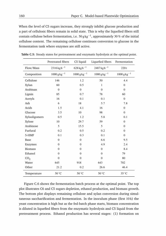
160 Paper C. Model-based Plantwide Optimization
When the level of C5 sugars increase, they strongly inhibit glucose production and
a part of cellulosic fibers remain in solid state. This is why the liquefied fibers still
contain cellulose before fermentation, i.e. 50 gkg−1, approximately 30 % of the initial
cellulose content. The remaining cellulose continues conversion to glucose in the
fermentation tank where enzymes are still active.
Table C.5: Steady states for pretreatment and enzymatic hydrolysis at the optimal point.
Pretreated fibers C5 liquid Liquefied fibers Fermentation
Flow/Mass 2316 kgh−1 628 kgh−1 2487 kgh−1 220 t
Composition 1000 gkg−1 1000 gkg−1 1000 gkg−1 1000 gkg−1
Cellulose 146 1.2 50 4.4
Xylan 60 0.5 1 0
Arabinan 0 0 0 0
Lignin 85 0.7 78 60
Acetyls 16 0.1 0.1 0
Ash 6 18 5.7 7.8
Acids 1.5 4.1 16 0
Glucose 3.5 10 98 0
Xylooligomers 0.5 1.2 5.8 0.1
Xylose 10 29.7 59 0
Arabinose 5 15.5 5 0
Furfural 0.2 0.5 0.2 0
5-HMF 0.1 0.3 0.1 0
Base 0 0 6.6 9.5
Enzymes 0 0 4.9 2.4
Biomass 0 0 0 8.4
Ethanol 0 0 0 79
CO2 0 0 0 80
Water 645 918 643 702
Other 21.2 0.2 26.6 46.4
Temperature 50 ◦C 50 ◦C 50 ◦C 35 ◦C
Figure C.6 shows the fermentation batch process at the optimal point. The top
plot illustrates C6 and C5 sugars depletion, ethanol production, and biomass growth.
The bottom plot displays remaining cellulose and xylan conversion during simul-
taneous saccharification and fermentation. In the inoculum phase (first 10 h) the
yeast concentration is high but as the fed-batch phase starts, biomass concentration
is diluted in liquefied fibers from the enzymatic hydrolysis and C5 liquid from the
pretreatment process. Ethanol production has several stages: (1) formation on
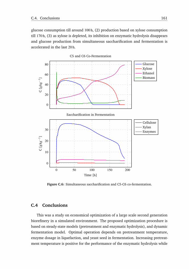
C.4. Conclusions 161
glucose consumption till around 100 h, (2) production based on xylose consumption
till 170 h, (3) as xylose is depleted, its inhibition on enzymatic hydrolysis disappears
and glucose production from simultaneous saccharification and fermentation is
accelerated in the last 20 h.
0
20
40
60
80
C[g
kg−
1 ]
C5 and C6 Co-Fermentation
GlucoseXyloseEthanolBiomass
0 50 100 150 200
0
10
20
30
Time [h]
C[g
kg−
1 ]
Saccharification in Fermentation
CelluloseXylanEnzymes
Figure C.6: Simultaneous saccharification and C5-C6 co-fermentation.
C.4 Conclusions
This was a study on economical optimization of a large scale second generation
biorefinery in a simulated environment. The proposed optimization procedure is
based on steady-state models (pretreatment and enzymatic hydrolysis), and dynamic
fermentation model. Optimal operation depends on pretreatment temperature,
enzyme dosage in liquefaction, and yeast seed in fermentation. Increasing pretreat-
ment temperature is positive for the performance of the enzymatic hydrolysis while

162 Paper C. Model-based Plantwide Optimization
negative for ethanol yield. Uncertainties in kinetics of pretreatment, liquefaction
and fermentation were negligible on the economic objective function around the
optimal operational point. The main source of uncertainty was found to be the inflow
feed composition. The optimization layer reduced the uncertainty and flattened
the profit curve allowing a wider range of operation with higher profit. The overall
improvement of the optimization layer is of approximately 18 % over the traditional
plant.
Supplementary Material
Introduction
This supplementary material summarizes the dynamic mathematical models for
pretreatment and enzymatic hydrolysis used in the plantwide optimization study.
These models are necessary for calculating the steady state values. Due to the high
complexity and model nonlinearities, an analytical steady state solution is hard to
find. The alternative is to run a sufficiently long simulation with constant inputs and
grab the final stabilized state values.
Mathematical Models
Pretreatment
The pretreatment process occurs in a large horizontal thermal reactor, which
is pressurized with steam till the necessary reaction pressure/temperature. The
following parameter distributed equation models the biomass transportation from
inlet to outlet subject to conversion due to the steam temperature [5]:
dCk
dt=
uz
δz(Ck−1−Ck)+Rk (C.49)
Ck is the composition vector in central cell k, Ck−1 is the composition vector from the
western neighbor, and Rk is the reaction rate vector from current cell k. Movement
from west to east (left to right) is assumed.
The pretreatment conversion mechanism is shown in Figure C.7. The reaction
rates for building vector Rk are modeled as first order Arrhenius type reactions, and
are detailed in Prunescu et al. [5]. A summary is given below:
• Glucose production due to cellulose hydrolysis:
rG = kG exp(− EG
R ·TK
)CCS (C.50)
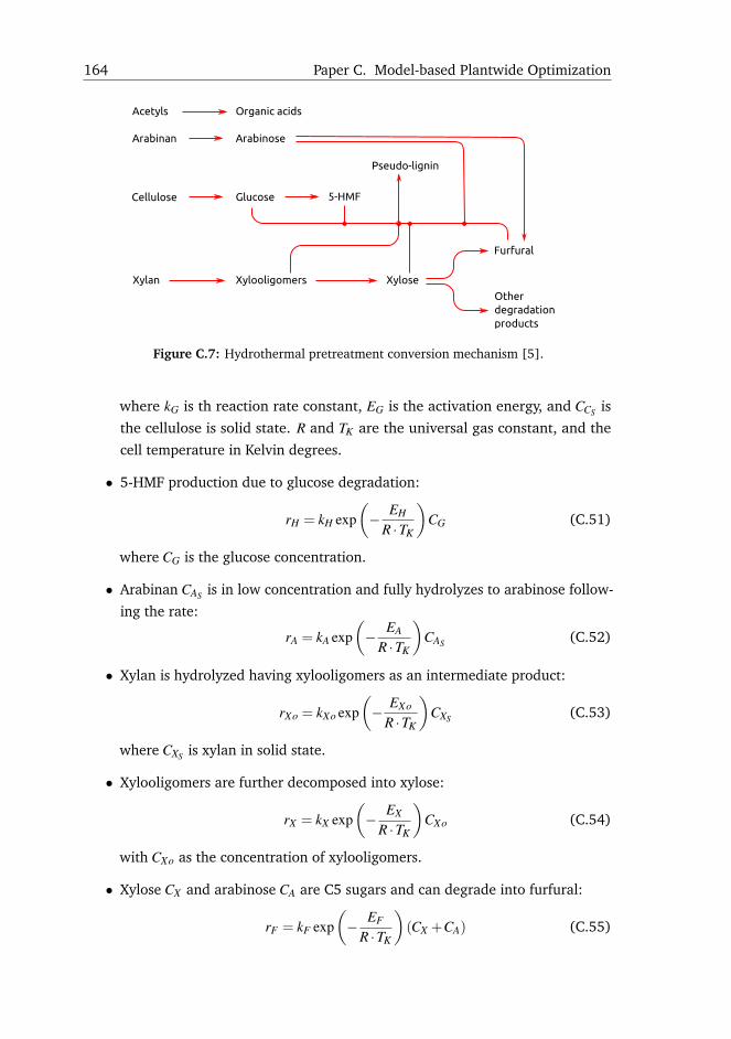
164 Paper C. Model-based Plantwide Optimization
Figure C.7: Hydrothermal pretreatment conversion mechanism [5].
where kG is th reaction rate constant, EG is the activation energy, and CCS is
the cellulose is solid state. R and TK are the universal gas constant, and the
cell temperature in Kelvin degrees.
• 5-HMF production due to glucose degradation:
rH = kH exp(− EH
R ·TK
)CG (C.51)
where CG is the glucose concentration.
• Arabinan CAS is in low concentration and fully hydrolyzes to arabinose follow-
ing the rate:
rA = kA exp(− EA
R ·TK
)CAS (C.52)
• Xylan is hydrolyzed having xylooligomers as an intermediate product:
rXo = kXo exp(− EXo
R ·TK
)CXS (C.53)
where CXS is xylan in solid state.
• Xylooligomers are further decomposed into xylose:
rX = kX exp(− EX
R ·TK
)CXo (C.54)
with CXo as the concentration of xylooligomers.
• Xylose CX and arabinose CA are C5 sugars and can degrade into furfural:
rF = kF exp(− EF
R ·TK
)(CX +CA) (C.55)
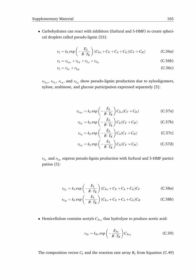
Supplementary Material 165
• Carbohydrates can react with inhibitors (furfural and 5-HMF) to create spheri-
cal droplets called pseudo-lignin [53]:
rL = kL exp(− EL
R ·TK
)(CXo +CX +CA +CG)(CF +CH) (C.56a)
rL = rLXo + rLX + rLA + rLG (C.56b)
rL = rLF + rLH (C.56c)
rLXo , rLX , rLA , and rLG show pseudo-lignin production due to xylooligomers,
xylose, arabinose, and glucose participation expressed separately [5]:
rLXo = kL exp(− EL
R ·TK
)CXo(CF +CH) (C.57a)
rLX = kL exp(− EL
R ·TK
)CX (CF +CH) (C.57b)
rLA = kL exp(− EL
R ·TK
)CA(CF +CH) (C.57c)
rLG = kL exp(− EL
R ·TK
)CG(CF +CH) (C.57d)
rLF and rLH express pseudo-lignin production with furfural and 5-HMF partici-
pation [5]:
rLF = kL exp(− EL
R ·TK
)(CXo +CX +CA +CG)CF (C.58a)
rLH = kL exp(− EL
R ·TK
)(CXo +CX +CA +CG)CH (C.58b)
• Hemicellulose contains acetyls CAcS that hydrolyze to produce acetic acid:
rAc = kAc exp(− EAc
R ·TK
)CAcS (C.59)
The composition vector Ck and the reaction rate array Rk from Equation (C.49)
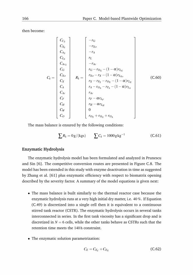
166 Paper C. Model-based Plantwide Optimization
then become:
Ck =
CCS
CXS
CAS
CLS
CAcS
CG
CXo
CX
CA
CAc
CF
CH
CW
CO
Rk =
−rG
−rXo
−rA
rL
−rAc
rG− rOG − (1−α)rLG
rXo− rX − (1−α)rLXo
rX − rFX − rOX − (1−α)rLX
rA− rOA − rFA − (1−α)rLA
rAc
rF −αrLF
rH −αrLH
0rOX + rOG + rOA
(C.60)
The mass balance is ensured by the following conditions:
∑Rk = 0g/(kgs) ∑Ck = 1000gkg−1 (C.61)
Enzymatic Hydrolysis
The enzymatic hydrolysis model has been formulated and analyzed in Prunescu
and Sin [6]. The competitive conversion routes are presented in Figure C.8. The
model has been extended in this study with enzyme deactivation in time as suggested
by Zhang et al. [61] plus enzymatic efficiency with respect to biomatrix opening
described by the severity factor. A summary of the model equations is given next:
• The mass balance is built similarly to the thermal reactor case because the
enzymatic hydrolysis runs at a very high initial dry matter, i.e. 40 %. If Equation
(C.49) is discretized into a single cell then it is equivalent to a continuous
stirred tank reactor (CSTR). The enzymatic hydrolysis occurs in several tanks
interconnected in series. In the first tank viscosity has a significant drop and is
discretized in N = 6 cells, while the other tanks behave as CSTRs such that the
retention time meets the 140 h constraint.
• The enzymatic solution parametrization:
CE =CEC +CEX (C.62)
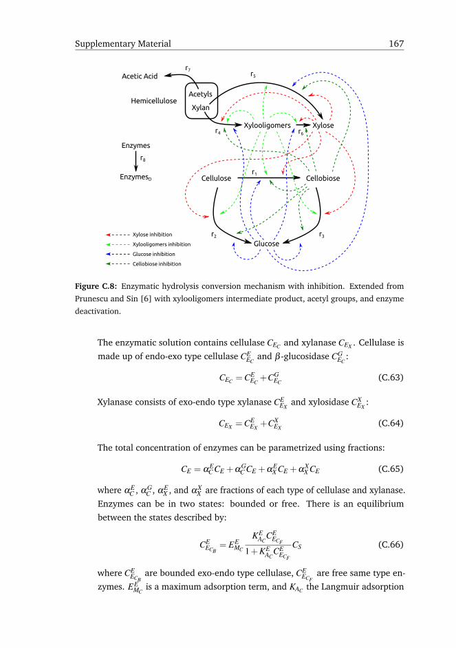
Supplementary Material 167
Figure C.8: Enzymatic hydrolysis conversion mechanism with inhibition. Extended from
Prunescu and Sin [6] with xylooligomers intermediate product, acetyl groups, and enzyme
deactivation.
The enzymatic solution contains cellulase CEC and xylanase CEX . Cellulase is
made up of endo-exo type cellulase CEEC
and β -glucosidase CGEC
:
CEC =CEEC
+CGEC
(C.63)
Xylanase consists of exo-endo type xylanase CEEX
and xylosidase CXEX
:
CEX =CEEX
+CXEX
(C.64)
The total concentration of enzymes can be parametrized using fractions:
CE = αEC CE +αG
C CE +αEX CE +αX
X CE (C.65)
where αEC , αG
C , αEX , and αX
X are fractions of each type of cellulase and xylanase.
Enzymes can be in two states: bounded or free. There is an equilibrium
between the states described by:
CEECB
= EEMC
KEAC
CEECF
1+KEAC
CEECF
CS (C.66)
where CEECB
are bounded exo-endo type cellulase, CEECF
are free same type en-
zymes. EEMC
is a maximum adsorption term, and KAC the Langmuir adsorption

168 Paper C. Model-based Plantwide Optimization
constant. CS is the solid substrate that enzymes are bound to. Equation (C.66)
applies to all types of enzymes, i.e. β -glucosidase, endo-exo type xylanase,
and xylosidase.
• Kinetic modeling of the reaction rates from Figure C.8: Reaction r1 describes
cellulose hydrolysis to cellobiose:
r1 =K1η(T, pH,r)CE
ECBCCS
1+ CCIC1
+ CXIX1
+ CGIG1
+ CXoIXo1
+ CEthIEth1
(C.67)
K1 is the reaction rate, η(T, pH,r) is the temperature, pH, and severity depen-
dency of the enzymatic activity, CEECB
are the bounded exo-endo type cellulase,
and CCS is the concentration of solid cellulose. The reaction rate is inhibited by
cellobiose CC, xylose CX , xylooligomers CXo, and glucose CG through inhibition
terms IC1 , IX1 , IXo1 , and IG1 . In simultaneous saccharification and fermentation
(SSF) ethanol also inhibits cellobiose formation [96] modeled through IEth1 in
the above rate.
Cellulose is also decomposed straight to glucose by the action of both endo-exo
type enzymes and β -glucosidase:
r2 =K2η(T, pH,r)
(CE
ECB+CG
ECB
)CCS
1+ CCIC2
+ CXoIXo2
+ CXIX2
+ CGIG2
+ CEthIEth2
(C.68)
Cellobiose decomposes to glucose:
r3 =K3η(T, pH)CG
ECFCC
I3
(1+ CXo
IXo3+ CX
IX3+ CG
IG3+ CEth
IEth3
)+CC
(C.69)
Xylan hydrolysis follows a similar path. Xylan form a xylooligomers pool:
r4 =K4η(T, pH)CE
EXBCXS
1+ CCIC4
+ CXoIXo4
+ CXIX4
+ CGIG4
+ CEthIEth4
(C.70)
Xylan could also be decomposed straight to xylose in a smaller amount:
r5 =K5η(T, pH)
(CE
EXB+CX
EXB
)CXS
1+ CCIC5
+ CXoIXo5
+ CXIX5
+ CGIG5
+ CEthIEth5
(C.71)
Xylooligomers are further decomposed to xylose:
r6 =K6η(T, pH)CX
EXFCXo
I6
(1+ CC
IC6+ CX
IX6+ CG
IG6+ CEth
IEth6
)+CXo
(C.72)
Supplementary Material 169
Acetic acid production happens due to acetyls being released along with xylan
hydrolysis:
r7 = βAc(r4 + r5) (C.73)
Enzymes deactivate in time due to thermal inactivation and exposure to ethanol
[61]:
r8 =−K8C2E (C.74)
• pH is modeled based on the charge balance equation:
[H+]− [OH−]− [Ac−]+ [Na+] = 0 (C.75)
The hydrogen ion concentration is found as the solution to the charge balance
equation. The other ions are expressed using the states and dissociation
constants. pH is then defined as:
pH =− log10[H+] (C.76)
• The enzymatic activity is a function of temperature, pH and severity factor as
illustrated in Figure C.9:
η(T, pH,r) = ηT (T )ηp(pH)ηr(r) (C.77)
The temperature and pH dependency are determined based on linear inter-
polation of experimental tabular data, and have the shape of a bell with a
single optimal peak [57, 58]. The severity [50, 97] dependency illustrate the
biomatrix opening, and models how hard the enzymes can access the cellulosic
and hemicellulosic fibers due to the physical structure of the biomass. The
severity factor is a function of retention time and temperature [97]. Insufficient
pretreatment can block enzymes accessibility to fibers.
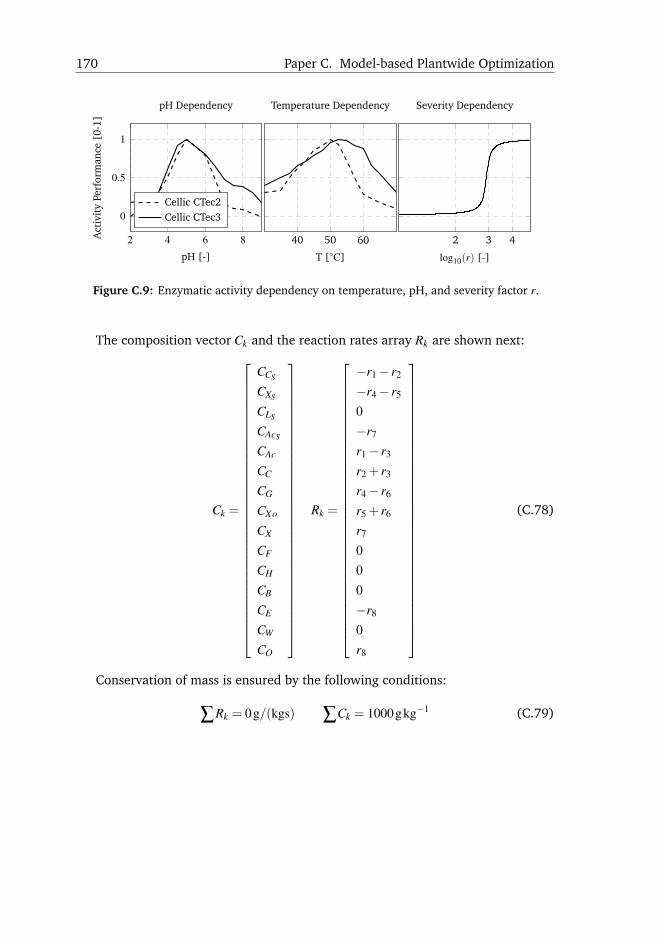
170 Paper C. Model-based Plantwide Optimization
2 4 6 8
0
0.5
1
pH [-]
Act
ivit
yPe
rfor
man
ce[0
-1]
pH Dependency
Cellic CTec2Cellic CTec3
40 50 60
T [◦C]
Temperature Dependency
2 3 4
log10(r) [-]
Severity Dependency
Figure C.9: Enzymatic activity dependency on temperature, pH, and severity factor r.
The composition vector Ck and the reaction rates array Rk are shown next:
Ck =
CCS
CXS
CLS
CAcS
CAc
CC
CG
CXo
CX
CF
CH
CB
CE
CW
CO
Rk =
−r1− r2
−r4− r5
0−r7
r1− r3
r2 + r3
r4− r6
r5 + r6
r7
000−r8
0r8
(C.78)
Conservation of mass is ensured by the following conditions:
∑Rk = 0g/(kgs) ∑Ck = 1000gkg−1 (C.79)
Paper D
Modeling and L1 AdaptiveControl of Temperature inBiomass Pretreatment
Remus Mihail Prunescu1, Mogens Blanke*1, Gürkan Sin2
1Department of Electrical Engineering, Automation and Control Group, Technical
University of Denmark, Elektrovej Building 326, 2800, Kgs. Lyngby, Denmark
2CAPEC-PROCESS, Department of Chemical and Biochemical Engineering, Technical
University of Denmark, Søltofts Plads Buildings 227 and 229, 2800, Kgs. Lyngby,
Denmark
Abstract:
Biomass steam pretreatment is a key process in converting agricultural wastes to
bioethanol. The pretreatment occurs in a large pressurized tank called a thermal
reactor. Two key parameters influence the successfulness of the process: the reactor
temperature, and the retention time. A particle pump pressurizes untreated biomass
from atmospheric to reactor pressure with recycled steam from the reactor. This
paper formulates a steam mathematical model both for the thermal reactor and the
particle pump, which is then used to design an L1 adaptive output feedback controller
for the reactor temperature. As steam is recycled from the reactor to pressurize the
particle pump, pressure drops and the reactor temperature is disturbed. The main
control challenge is to reject these disturbances and keep a steady temperature. The
nonlinear process model embeds mass and energy balances, valve characteristics,
and enthalpy-pressure and pressure-temperature dependencies. Nonlinear feed-
forward terms are added in the control strategy. The process model, the control
strategy, the application of the L1 adaptive controller and its tuning method based
on minimizing a cost function represent novelties of this paper.
*Principal corresponding author. Tel.: +45 45253565; E-mail: [email protected]
172 Paper D. Modeling and L1 Adaptive Control of Pretreatment Temperature
D.1 Introduction
Biofuel receives more interest lately due to the increase in oil price worldwide,
and due to the green commitments that governments have taken for reducing
emissions of greenhouse gases, e.g. the Kyoto protocol [19]. In this context, many
private companies and governments invest in large scale biofuel production plants
[3].
The conversion of agricultural wastes to ethanol requires several steps. A thermal
reactor pretreats the biomass by removing the wooden part of the plant, i.e. lignin,
and creates a mixture rich in cellulose fibers. Enzymes breakdown the fibers in
a liquefaction process and large tanks store the resulting slurry for fermentation.
Distillation columns recover ethanol, which is used in preparation of fuel blends. Two
more by-products are obtained: lignin, which is recovered from the pretreatment
process as bio-pallets and co-combusted in a power plant; and C5 molasses, which is
a syrup rich in nutrients and sold to farmers for feeding their animals. The entire
biofuel production cycle is thoroughly described in [3, 4].
The biomass pretreatment process is the key step in biofuel production. There
are various methods of pretreatment, most of them involving steam, strong acids or
weak acids [121]. The effects of different pretreatment methods were investigated
in [44, 122]. A combination of steam and weak acids gives the best results. Also, to
reduce steam operating costs, refineries are integrated with a power plant following
the IBUS principle [4].
The steam pretreatment process occurs in a pressurized continuous thermal
reactor, which is preceded by a pressurization unit also known as a particle pump
[71]. Depending on the load, the particle pump releases an amount of biomass to
the thermal reactor with a certain frequency. The degree of pretreatment determines
the chemical composition of the outstream. Steam pretreatment started to be
investigated in [97] and an empirical pretreatment model for ethanol production
was formulated in [50]. Two key parameters of the process, i.e. retention time and
reactor temperature, are vital to an effective process.
Various disturbances have been identified for a large thermal reactor in [71],
among which the most important one is the particle pump operation cycle, which
is causing oscillations in the steam layer temperature. These oscillations further
disturb the temperature of the biomass layer, causing an irregular pretreatment
process. Temperature matters because a deviation of 10 ◦C can cause a drop of
10% in cellulose recovery [50]. A poor pretreatment can also lead to formation
of inhibitors that affect the downstream processes of enzymatic hydrolysis and
fermentation, or it could disturb the pH level of the outstream by releasing more

D.2. Process Description 173
or less acetic acid from the biomass. It is well known that enzymes are sensitive to
pH following a bell-shaped curve [123]. Therefore, the main control challenge in
this investigation is to reject any disturbances that affect the reactor temperature
in order to ensure a uniform temperature environment in the steam and biomass
layers.
To achieve this objective, an adaptive control strategy for the pretreatment
temperature is proposed in this article. First, a nonlinear model of the steam layer
is formulated from mass and energy balances, enthalpy-pressure and enthalpy-
temperature dependencies, and nonlinear valve characteristics. Disturbance sources
are also introduced, i.e. condensation of steam and uncertainties in the measurement
of recycled steam. The biomass load in the reactor is also a factor and the controller
will be tuned for a specific load and tested in another operational point. A disturbance
can take the system to multiple operational points and adaptation should improve
the control performances. Therefore, an adaptive control strategy is developed
based on the L1 adaptive output feedback controller. L1 adaptive control represents
the latest novelty in control theory [10]. Also, a new tuning method of the L1
controller is proposed in this paper based on minimizing the integral absolute error
(IAE) performance function. The modelling work, the application of the L1 adaptive
controller on a biomass pretreatment process and the tuning method of the controller
have not been reported earlier in the literature.
D.2 Process Description
The process has been described in [71] and is briefly reiterated in this section.
A process diagram is illustrated in Figure D.1. The particle pump receives small
amounts of soaked biomass and pressurizes them till the reactor pressure. Afterward,
the particle pump releases the biomass into the thermal reactor and the cycle
repeats. In the thermal reactor, the biomass is pushed horizontally by a snail. The
particle pump operates at various frequencies depending on the desired load of the
thermal reactor. A fast operation increases the load in the reactor assuming the snail
speed constant. When the load increases the available volume for the steam layer
diminishes. A reduced air volume can be pressurized faster by steam, so the time
constants of the system change according to the load.
It is assumed that the particle pump is pressurized only with recycled steam from
the reactor while the thermal reactor is pressurized only with fresh steam, which
enters the tank through the bottom. It is preferred to use recycled steam when
pressurizing the particle pump because it would create a pressure disturbance that
causes a burst of steam from the bottom, which would facilitate the breakdown of

174 Paper D. Modeling and L1 Adaptive Control of Pretreatment Temperature
ParticlePump
Thermal Reactor
PretreatedBiomass
SoakedBiomass
FreshSteam
EvacuationSteam
Recycle SteamQRS
QEPP
QFST R
QBiPP
PPP
PT R TT R
PFS
QRS
Figure D.1: Process diagram with instrumentation. Green arrows follow the biomass path
while red arrows indicate steam flow. There are 3 steam valves, i.e. QFS or fresh steam
valve, QRS or recycled steam valve and QE or evacuation valve. PPP, PT R and PFS measure
the pressure in the particle pump, thermal reactor and fresh steam pipe, respectively. TT R
indicates the reactor temperature.
soaked biomass leading to a more uniform pretreatment process.
The pressure in the particle pump and the pressure in the reactor are measured
as PPP and PT R. Another pressure sensor is positioned in the fresh steam pipe and
the measurement is denoted as PFS. The fresh steam arrives from a flash tank and
is assumed to be saturated. The temperature in the thermal reactor is of interest
and directly measured as TT R. The recycle steam flow is also measured as QRS and
is necessary to construct a feed-forward action. The steam layers from the particle
pump and thermal reactor are assumed to be uniform. There are 3 steam valves that
can be manipulated and their strokes are denoted as SEPP, SFS
T R and SRS.
D.3 Mathematical Model

D.3. Mathematical Model 175
Table D.1: Process model nomenclature.
States
mSPP Steam mass in particle pump (PP) kg
hSPP Specific steam enthalpy in PP kJkg−1
mST R Steam mass in thermal reactor (TR) kg
hST R Specific steam enthalpy in TR kJkg−1
mBPP Mass of biomass in PP kg
mBT R Mass of biomass in TR kg
Inputs
SFST R Stroke of fresh steam valve in TR %
SRS Stroke of recycle steam valve %
SEPP Stroke of evacuation valve in PP %
QBiPP Inflow of biomass in PP kgs−1
QBiT R Inflow of biomass in TR kgs−1
QBoT R Outflow of biomass from TR kgs−1
hSFS Fresh steam enthalpy kJkg−1
PFS Fresh steam pressure bar
Outputs
PPP Pressure in PP bar
PT R Pressure in TR bar
PA Atmospheric pressure bar
TPP Temperature in PP ◦C
TT R Temperature in TR ◦C
Auxiliary Variables
QRS Mass flow of recycled steam kgs−1
QEPP Mass outflow of steam from PP kgs−1
QFST R Mass inflow of fresh steam in TR kgs−1
ρSPP Density of steam in PP kgm−3
ρST R Density of steam in TR kgm−3
V SPP Steam volume in PP m3
V ST R Steam volume in TR m3
Constant Parameters
VPP Total volume of PP m3
176 Paper D. Modeling and L1 Adaptive Control of Pretreatment Temperature
VT R Total volume of TR m3
Disturbances
QCT R Condensing steam in TR kgs−1
QMRS Recycle steam measurement noise kgs−1
D.3.1 Process Model
The process model consists of mass and energy balances of the steam layer for
both the particle pump and the thermal reactor:
d(mSPP)
dt= QRS−QE
PP (D.1a)
d(mSPPhS
PP)
dt= QRShS
T R−QEPPhS
PP (D.1b)
d(mST R)
dt= QFS
T R−QRS−QCT R (D.1c)
d(mST RhS
T R)
dt= QFS
T RhSFS− (QRS +QC
T R)hST R (D.1d)
Equation (D.1a) is the particle pump steam mass balance and Equation (D.1b) is
the energy balance of the steam layer from the particle pump. All notations are
explained in Table D.1. Similarly, Equation (D.1c) shows the mass balance from the
thermal reactor and Equation (D.1d) contains the energy balance of the steam layer
in the reactor.
The mass of soaked biomass in both the particle pump and thermal reactor are
also tracked as it affects the available volume for steam expansion:
d(mBPP)
dt= QBi
PP−QBiT R (D.2a)
d(mBT R)
dt= QBi
T R−QBoT R (D.2b)
D.3.2 Valve Modelling
The valve characteristics can be retrieved from the valve manufacturer and shows
KV as a function of the valve opening or stroke S. KV represents the flow of steam
in m3 s−1 when the pressure drop across the valve is 1 bar. A typical characteristic is
displayed in Figure D.2 and can be accurately approximated by a cubic polynomial:
KV (S) = k3S3 + k2S2 + k1S+ k0 (D.3)
where ki are the polynomial coefficients and S is the valve stroke.
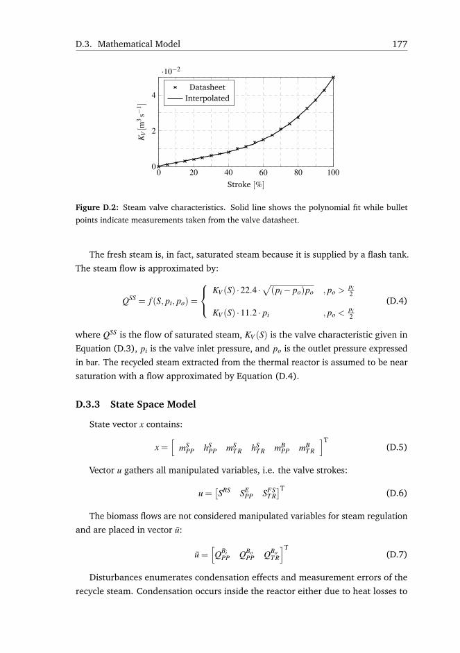
D.3. Mathematical Model 177
0 20 40 60 80 1000
2
4
·10−2
Stroke [%]
KV[m
3s−
1 ]
DatasheetInterpolated
Figure D.2: Steam valve characteristics. Solid line shows the polynomial fit while bullet
points indicate measurements taken from the valve datasheet.
The fresh steam is, in fact, saturated steam because it is supplied by a flash tank.
The steam flow is approximated by:
QSS = f (S, pi, po) =
KV (S) ·22.4 ·√(pi− po)po , po >
pi2
KV (S) ·11.2 · pi , po <pi2
(D.4)
where QSS is the flow of saturated steam, KV (S) is the valve characteristic given in
Equation (D.3), pi is the valve inlet pressure, and po is the outlet pressure expressed
in bar. The recycled steam extracted from the thermal reactor is assumed to be near
saturation with a flow approximated by Equation (D.4).
D.3.3 State Space Model
State vector x contains:
x =[
mSPP hS
PP mST R hS
T R mBPP mB
T R
]T(D.5)
Vector u gathers all manipulated variables, i.e. the valve strokes:
u =[SRS SE
PP SFST R]T
(D.6)
The biomass flows are not considered manipulated variables for steam regulation
and are placed in vector u:
u =[QBi
PP QBoPP QBo
T R
]T(D.7)
Disturbances enumerates condensation effects and measurement errors of the
recycle steam. Condensation occurs inside the reactor either due to heat losses to

178 Paper D. Modeling and L1 Adaptive Control of Pretreatment Temperature
the environment or because of temperature differences between the biomass and
the steam layer. Measurement errors in the recycle steam flow may appear due to its
fast and turbulent dynamics. Vector d comprises all disturbances:
d =[QC
T R QMRS]T
(D.8)
The steam volume in each container is found by subtracting the biomass volume
from the total volume:
VS =V −VB (D.9)
where VS is the steam volume, V is the total volume and VB is the biomass volume.
Steam volumes are gathered in vector v:
v =[V S
PP V ST R]T
(D.10)
Steam densities from both containers are placed into the following vector:
ρ =[ρS
PP ρST R]T
(D.11)
Steam density is found by dividing the mass of steam by volume. For example, the
steam density in the thermal reactor can be computed in the following way:
ρ2 =x3
v2(D.12)
where index 2 and 3 selects the corresponding element from vector ρ, x or v.
All pressure variables are gathered in vector p:
p = [PFS PPP PT R PA]T (D.13)
where PA is the outlet pressure of the evacuation valve, which is, in fact, atmospheric
pressure.
In case of saturated steam, one steam variable is sufficient to determine any of the
other variables. In case of wet or superheated steam, 2 steam variables are necessary
to determine its state. Steam properties are inferred from the IAPWS IF97 standard.
The fresh steam is saturated and its enthalpy is found from its pressure, which is
directly measured. The reactor pressure is determined from enthalpy and density
while the temperature is found from enthalpy and pressure. Figure D.3 displays
these steam properties. Pressure has a rather linear dependence with respect to
density and enthalpy (left plot). Nonlinearities are spotted in temperature variations
with respect to pressure in the wet steam region and in the saturation zone (right
plot).
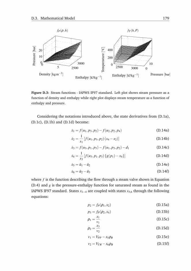
D.3. Mathematical Model 179
05 2500
30000
10
20
Density [kgm−3]Enthalpy [kJkg−1]
Pres
sure
[bar]
fP(ρ,h)
2500 3000 0100
200
400
Enthalpy [kJkg−1] Pressure [bar]
Tem
pera
ture
[◦C]
fT (h,P)
Figure D.3: Steam functions - IAPWS IF97 standard. Left plot shows steam pressure as a
function of density and enthalpy while right plot displays steam temperature as a function of
enthalpy and pressure.
Considering the notations introduced above, the state derivatives from (D.1a),
(D.1c), (D.1b) and (D.1d) become:
x1 = f (u1, p3, p2)− f (u2, p2, p4) (D.14a)
x2 =1x1
[ f (u1, p3, p2)(x4− x2)] (D.14b)
x3 = f (u3, p1, p3)− f (u1, p3, p2)−d1 (D.14c)
x4 =1x3
[ f (u3, p1, p3){g(p1)− x4}] (D.14d)
x5 = u1− u2 (D.14e)
x6 = u2− u3 (D.14f)
where f is the function describing the flow through a steam valve shown in Equation
(D.4) and g is the pressure-enthalpy function for saturated steam as found in the
IAPWS IF97 standard. States x1−4 are coupled with states x5,6 through the following
equations:
p2 = fP(ρ1,x2) (D.15a)
p3 = fP(ρ2,x4) (D.15b)
ρ1 =x1
v1(D.15c)
ρ2 =x3
v2(D.15d)
v1 =VPP− x5ρB (D.15e)
v2 =VT R− x6ρB (D.15f)
180 Paper D. Modeling and L1 Adaptive Control of Pretreatment Temperature
where ρB is the soaked biomass density set to 1000 kgm−3.
The model outputs are gathered in vector y and comprise the pressure and
temperature in both process units:
y = [pPP pT R TPP TT R]T (D.16)
where TPP and TT R are calculated as:
y3 = fT (x2, p2) (D.17a)
y4 = fT (x4, p3) (D.17b)
Overall, a nonlinear model with 6 states, 3 inputs and 4 outputs is obtained.
D.3.4 Open Loop Simulation
An open loop simulation is prepared in order to observe the system response.
The simulation scenario is synthesized in Table D.2.
Table D.2: Open loop simulation scenario.
Time [s] QFS [%] QRS [%] QEPP [%]
0 0 0 0
10 100 0 0
30 0 0 0
50 0 100 0
70 0 0 0
90 0 0 100
110 0 0 0
The reactor fresh steam valve is fully opened at time t = 10s for 20 s. The recycle
steam valve is fully opened at time t = 50s for another 20 s. The particle pump
evacuation valve is opened at time t = 90s for the last 20 s of the simulation. The
results are plotted in Figure D.4. Pressurization of the thermal reactor takes a much
longer time than the particle pump because it has a larger volume. The reactor
pressure resembles a second order system response while the temperature could
be approximated by a first order response. The particle pump pressurizes in only
several seconds and the pressure in both the reactor and the particle pump equalize.
There is a small drop in pressure in the reactor because steam is extracted in order
to pressurize the particle pump. These disturbances need to be rejected and ensure
a steady temperature in the process.
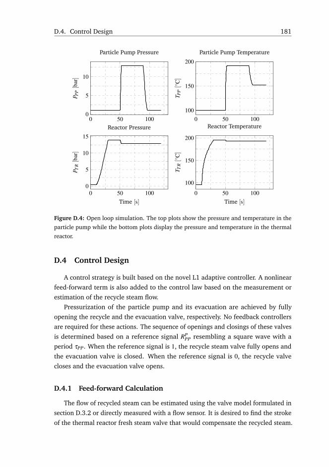
D.4. Control Design 181
0 50 1000
5
10P P
P[b
ar]
Particle Pump Pressure
0 50 100100
150
200
T PP[◦
C]
Particle Pump Temperature
0 50 1000
5
10
15
Time [s]
P TR[b
ar]
Reactor Pressure
0 50 100
100
150
200
Time [s]
T TR[◦
C]
Reactor Temperature
Figure D.4: Open loop simulation. The top plots show the pressure and temperature in the
particle pump while the bottom plots display the pressure and temperature in the thermal
reactor.
D.4 Control Design
A control strategy is built based on the novel L1 adaptive controller. A nonlinear
feed-forward term is also added to the control law based on the measurement or
estimation of the recycle steam flow.
Pressurization of the particle pump and its evacuation are achieved by fully
opening the recycle and the evacuation valve, respectively. No feedback controllers
are required for these actions. The sequence of openings and closings of these valves
is determined based on a reference signal RPPP resembling a square wave with a
period τPP. When the reference signal is 1, the recycle steam valve fully opens and
the evacuation valve is closed. When the reference signal is 0, the recycle valve
closes and the evacuation valve opens.
D.4.1 Feed-forward Calculation
The flow of recycled steam can be estimated using the valve model formulated in
section D.3.2 or directly measured with a flow sensor. It is desired to find the stroke
of the thermal reactor fresh steam valve that would compensate the recycled steam.
182 Paper D. Modeling and L1 Adaptive Control of Pretreatment Temperature
The stroke of the thermal reactor fresh steam valve is different than the stroke of
the recycle valve because the inlet and outlet pressures are different. From Equation
(D.4) the valve characteristic KV can be determined:
KV (t) =
QRS(t)
22.4·√
(pi−po)po, po >
pi2
QRS(t)11.2·pi
, po <pi2
(D.18)
The valve stroke S can be expressed as a function of the valve characteristic KV
by conducting the inverse of function (D.3). However, for simplification, a linear
characteristic is used for this computation:
SFF(KV (t)) =100KV (t)
0.05(D.19)
where 0.05 is the steam volumetric flow (in m3 s−1) when the valve is 100% open
with 1 bar pressure drop.
The stroke SFF is fed-forward through a trust gain KFF . The feed-forward control
signal becomes:
uFF(t) = KFF SFF(t) (D.20)
In this application, the trust gain KFF is set to 1 but could be reduced for a more
conservative feed-forward action.
D.4.2 L1 Adaptive Control
Figure D.5 shows the system in closed loop with an L1 adaptive output feedback
controller. The pressurization of the particle pump is shown in the upper part of
the figure. There is no feedback action because the pressure in the particle pump
should equalize the pressure in the reactor and this objective can be achieved by
fully opening the recycle steam valve. The L1 output feedback control strategy is
designed for temperature regulation and only one measurement is considered, i.e.
TT R. The manipulated variable is the fresh steam valve stroke, i.e. SFST R. Therefore,
the control object becomes a SISO model.
The L1 output feedback controller consists of an output predictor, an adaptation
law and a control filter C(s) [10, 124]. The classical model reference adaptive
controller implies a compromise between adaptation and robustness. Moreover,
there are no trivial ways of finding a suitable adaptation gain. The L1 adaptive
controller separates robustness from fast adaptation by introducing a filter C(s) in
the control channel. The analysis of the new controller i.e. the computation of the
uniform bounds on outputs and control signals, is performed using the L1 norm,
hence the name of L1 adaptive controller.
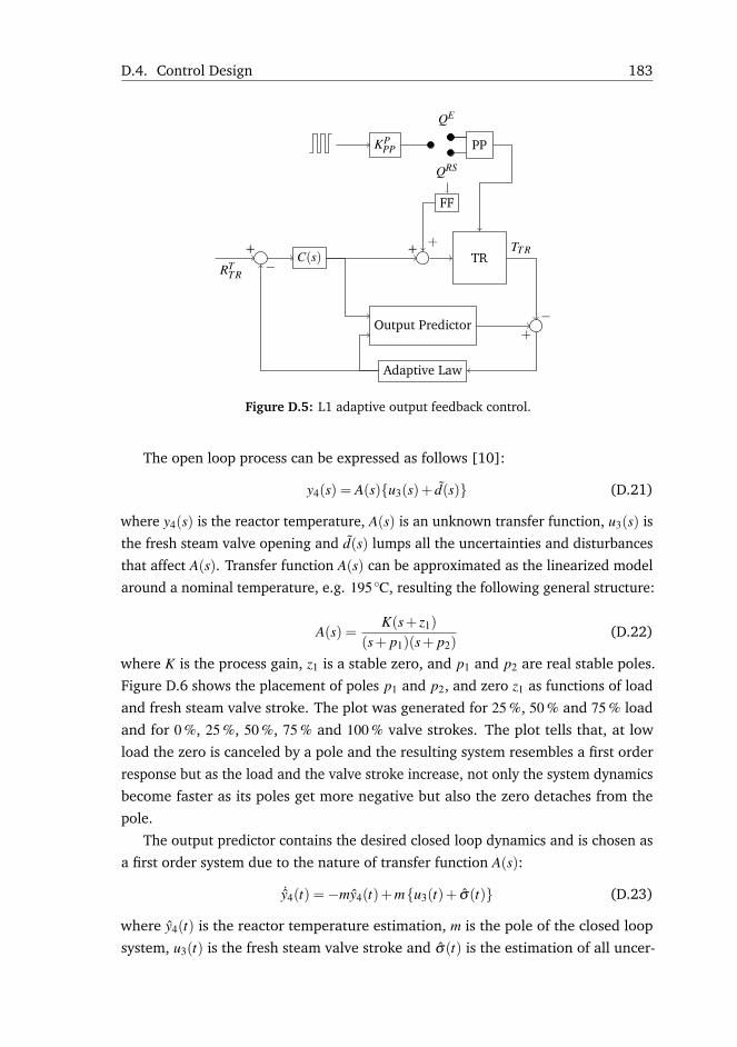
D.4. Control Design 183
C(s) TR
PP
RTT R
+ +
Output Predictor
Adaptive Law
TT R
−+
−
KPPP
QRS
QE
FF
+
Figure D.5: L1 adaptive output feedback control.
The open loop process can be expressed as follows [10]:
y4(s) = A(s){u3(s)+ d(s)} (D.21)
where y4(s) is the reactor temperature, A(s) is an unknown transfer function, u3(s) is
the fresh steam valve opening and d(s) lumps all the uncertainties and disturbances
that affect A(s). Transfer function A(s) can be approximated as the linearized model
around a nominal temperature, e.g. 195 ◦C, resulting the following general structure:
A(s) =K(s+ z1)
(s+ p1)(s+ p2)(D.22)
where K is the process gain, z1 is a stable zero, and p1 and p2 are real stable poles.
Figure D.6 shows the placement of poles p1 and p2, and zero z1 as functions of load
and fresh steam valve stroke. The plot was generated for 25 %, 50 % and 75 % load
and for 0 %, 25 %, 50 %, 75 % and 100 % valve strokes. The plot tells that, at low
load the zero is canceled by a pole and the resulting system resembles a first order
response but as the load and the valve stroke increase, not only the system dynamics
become faster as its poles get more negative but also the zero detaches from the
pole.
The output predictor contains the desired closed loop dynamics and is chosen as
a first order system due to the nature of transfer function A(s):
˙y4(t) =−my4(t)+m{u3(t)+ σ(t)} (D.23)
where y4(t) is the reactor temperature estimation, m is the pole of the closed loop
system, u3(t) is the fresh steam valve stroke and σ(t) is the estimation of all uncer-

184 Paper D. Modeling and L1 Adaptive Control of Pretreatment Temperature
0
50
100 020
4060
80100
−0.2
−0.1
0
Load [%] SFST R [%]
p,z
[rad
s−1 ]
p1
p2
z1
Figure D.6: Poles and zero migration as a function of load and recycle steam valve stroke.
tainties and unmodeled dynamics. In frequency domain, the model reference system
is denoted as:
M(s) =m
s+m(D.24)
System (D.21) can be rewritten in terms of the model reference system [10]:
y4(s) = M(s){u3(s)+σ(s)} (D.25)
where σ(s) is identified as:
σ(s) ={A(s)−M(s)}u3(s)+A(s)d(s)
M(s)(D.26)
The idea is to cancel uncertainties σ(s) with the help of the control signal u3(s).
Therefore, the control signal is defined as [10]:
u3(s) =C(s){r(s)− σ(s)} (D.27)
where C(s) is chosen in this application as a first order filter:
C(s) =c
s+ c(D.28)
If Equation (D.27) is substituted in (D.25) then:
y4(s) = M(s)C(s)r(s)+M(s){σ(s)−C(s)σ(s)} (D.29)
If σ(s) is perfectly estimated then σ(s) = σ(s) and the disturbances will be rejected
only in the bandwidth of C(s).
D.4. Control Design 185
In [10] the adaptation law is implemented as a projection algorithm. In this
application, because there is only one parameter to estimate, the adaptation law is
simplified to an integrator:˙σ(t) =−Γy4(t) (D.30)
where y4(t) = y4(t)−y4(t) is the estimation error of the output and Γ is the integrator
gain.
The resulting L1 adaptive output feedback controller has 3 tuning parameters, i.e.
the desired closed loop dynamics m, the adaptation gain Γ and the eigenfrequency
of the control filter c.
The reference model and the control signal filter can be designed systematically
[125]. Assuming perfect knowledge of disturbances, an ideal system y4(s) can be
built and used for tuning [125]:
y4(s) = H(s)C(s)r(s)+H(s){1−C(s)}d(s) (D.31)
where H(s)C(s) is the transfer function from r(s) to y4(s) and H(s) is defined as:
H(s) =A(s)M(s)
C(s)A(s)+{1−C(s)}M(s)(D.32)
Parameters m and c must be chosen such that H(s) is stable and the following L1
norm holds [10]:
||G(s)||L1L < 1 (D.33)
where G(s) = H(s){1−C(s)} is the transfer function from d(s) to y4(s) and L is the
Lipschitz constant required to guarantee BIBO stability (Lemma 4.1.1 in [10]).
In this application, parameters m, c and Γ are found by minimizing the integral
absolute error (IAE) function:
minm,c,Γ
∞∫0
|r(t)− y4(t)| (D.34)
where r(t)− y4(t) is the tracking error and y4(t) is the output of the nonlinear model.
A numerical search procedure is instantiated to obtain parameters m, c and
Γ. The simulation scenario for minimizing the objective function contains the
normal operation cycle, i.e. the particle pump extracting steam from the reactor,
which causes a disturbance in the reactor temperature. Therefore, the controller
is optimized for disturbance rejection. The objective function (D.34) cannot be
minimized analytically due to the complexity of the nonlinear model. The numerical
search procedure performs various simulations in closed loop, for each simulation
evaluating the IAE function from (D.34). The search algorithm is initialized by
following the tuning procedure shown in [12]. A temperature reference of 195 ◦C
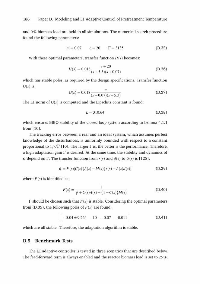
186 Paper D. Modeling and L1 Adaptive Control of Pretreatment Temperature
and 0 % biomass load are held in all simulations. The numerical search procedure
found the following parameters:
m = 0.07 c = 20 Γ = 3135 (D.35)
With these optimal parameters, transfer function H(s) becomes:
H(s) = 0.018s+20
(s+5.3)(s+0.07)(D.36)
which has stable poles, as required by the design specifications. Transfer function
G(s) is:
G(s) = 0.018s
(s+0.07)(s+5.3)(D.37)
The L1 norm of G(s) is computed and the Lipschitz constant is found:
L = 310.64 (D.38)
which ensures BIBO stability of the closed loop system according to Lemma 4.1.1
from [10].
The tracking error between a real and an ideal system, which assumes perfect
knowledge of the disturbances, is uniformly bounded with respect to a constant
proportional to 1/√
Γ [10]. The larger Γ is, the better is the performance. Therefore,
a high adaptation gain Γ is desired. At the same time, the stability and dynamics of
σ depend on Γ. The transfer function from r(s) and d(s) to σ(s) is [125]:
σ = F(s)[C(s){A(s)−M(s)}r(s)+A(s)d(s)] (D.39)
where F(s) is identified as:
F(s) =1
sΓ +C(s)A(s)+{1−C(s)}M(s)
(D.40)
Γ should be chosen such that F(s) is stable. Considering the optimal parameters
from (D.35), the following poles of F(s) are found:[−5.04±9.26i −10 −0.07 −0.011
](D.41)
which are all stable. Therefore, the adaptation algorithm is stable.
D.5 Benchmark Tests
The L1 adaptive controller is tested in three scenarios that are described below.
The feed-forward term is always enabled and the reactor biomass load is set to 25 %.
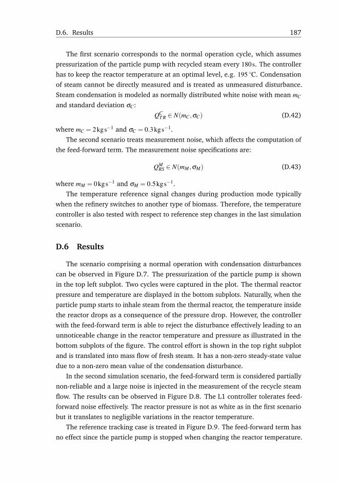
D.6. Results 187
The first scenario corresponds to the normal operation cycle, which assumes
pressurization of the particle pump with recycled steam every 180s. The controller
has to keep the reactor temperature at an optimal level, e.g. 195 ◦C. Condensation
of steam cannot be directly measured and is treated as unmeasured disturbance.
Steam condensation is modeled as normally distributed white noise with mean mC
and standard deviation σC:
QCT R ∈ N(mC,σC) (D.42)
where mC = 2kgs−1 and σC = 0.3kgs−1.
The second scenario treats measurement noise, which affects the computation of
the feed-forward term. The measurement noise specifications are:
QMRS ∈ N(mM,σM) (D.43)
where mM = 0kgs−1 and σM = 0.5kgs−1.
The temperature reference signal changes during production mode typically
when the refinery switches to another type of biomass. Therefore, the temperature
controller is also tested with respect to reference step changes in the last simulation
scenario.
D.6 Results
The scenario comprising a normal operation with condensation disturbances
can be observed in Figure D.7. The pressurization of the particle pump is shown
in the top left subplot. Two cycles were captured in the plot. The thermal reactor
pressure and temperature are displayed in the bottom subplots. Naturally, when the
particle pump starts to inhale steam from the thermal reactor, the temperature inside
the reactor drops as a consequence of the pressure drop. However, the controller
with the feed-forward term is able to reject the disturbance effectively leading to an
unnoticeable change in the reactor temperature and pressure as illustrated in the
bottom subplots of the figure. The control effort is shown in the top right subplot
and is translated into mass flow of fresh steam. It has a non-zero steady-state value
due to a non-zero mean value of the condensation disturbance.
In the second simulation scenario, the feed-forward term is considered partially
non-reliable and a large noise is injected in the measurement of the recycle steam
flow. The results can be observed in Figure D.8. The L1 controller tolerates feed-
forward noise effectively. The reactor pressure is not as white as in the first scenario
but it translates to negligible variations in the reactor temperature.
The reference tracking case is treated in Figure D.9. The feed-forward term has
no effect since the particle pump is stopped when changing the reactor temperature.
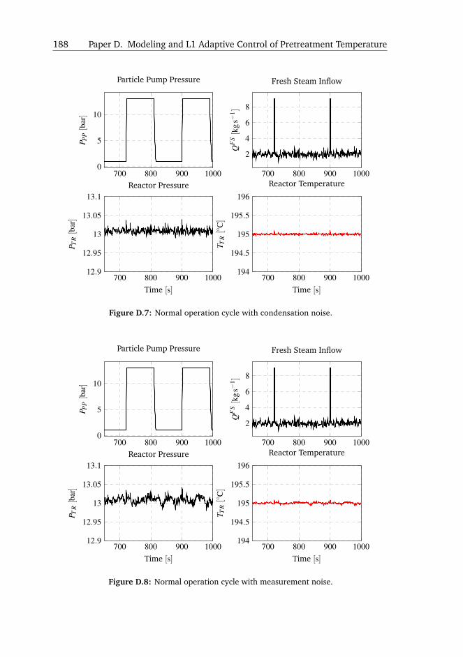
188 Paper D. Modeling and L1 Adaptive Control of Pretreatment Temperature
700 800 900 10000
5
10
P PP[b
ar]
Particle Pump Pressure
700 800 900 1000
2
4
6
8
QF
S[k
gs−
1 ]
Fresh Steam Inflow
700 800 900 100012.9
12.95
13
13.05
13.1
Time [s]
P TR[b
ar]
Reactor Pressure
700 800 900 1000194
194.5
195
195.5
196
Time [s]
T TR[◦
C]
Reactor Temperature
Figure D.7: Normal operation cycle with condensation noise.
700 800 900 10000
5
10
P PP[b
ar]
Particle Pump Pressure
700 800 900 1000
2
4
6
8
QF
S[k
gs−
1 ]
Fresh Steam Inflow
700 800 900 100012.9
12.95
13
13.05
13.1
Time [s]
P TR[b
ar]
Reactor Pressure
700 800 900 1000194
194.5
195
195.5
196
Time [s]
T TR[◦
C]
Reactor Temperature
Figure D.8: Normal operation cycle with measurement noise.
D.7. Conclusions 189
0 200 400 600 8000.8
0.9
1
1.1P P
P[b
ar]
Particle Pump Pressure
0 200 400 600 8000
5
QF
S[k
gs−
1 ]
Fresh Steam Inflow
0 200 400 600 800
12
14
Time [s]
P TR[b
ar]
Reactor Pressure
0 200 400 600 800190
195
200
Time [s]
T TR[◦
C]
Reactor Temperature
Figure D.9: Reference tracking with condensation noise.
Cooling the reactor is performed by interrupting the supply of fresh steam. The
L1 adaptive controller has good performances changing the temperature in less
than 1 min, which is satisfactory since temperature set point changes do not occur
frequently in production mode.
D.7 Conclusions
For the first time, to our knowledge, a steam layer model has been formulated
for a particle pump connected to a thermal reactor in biomass pretreatment. The
process model embeds nonlinear valve characteristics and steam states dependencies,
e.g. pressure, temperature, enthalpy and density.
The developed control strategy based on the novel L1 adaptive output feedback
controller proved to have very good performances in all simulation scenarios. Mea-
surement noise that affects the feed-forward term and condensation disturbances
were handled satisfactory. The application of such a controller to regulate the tem-
perature in a biomass pretreatment reactor has not been reported earlier in the
literature.
The last achievement of the paper is the tuning method of the L1 adaptive
controller. It proved successfully to formulate the tuning of the controller as an
190 Paper D. Modeling and L1 Adaptive Control of Pretreatment Temperature
optimization problem. The integral absolute error (IAE) has been used as an objective
function and the determined controller parameters proved to give satisfactory results
in simulation.
The temperature controller developed in this paper is part of an inner control
loop layer of a biorefinery. The temperature setpoint will be given by an outer
control loop layer that is using the pretreated biomass composition as feedback. The
objective is to obtain a steady pretreatment process and any variations in biomass
composition or type can be rejected by changing the temperature in the reactor.
Paper E
Modeling and L1 AdaptiveControl of pH in BioethanolEnzymatic Process
Remus Mihail Prunescu1, Mogens Blanke*1, Gürkan Sin2
1Department of Electrical Engineering, Automation and Control Group, Technical
University of Denmark, Elektrovej Building 326, 2800, Kgs. Lyngby, Denmark
2CAPEC-PROCESS, Department of Chemical and Biochemical Engineering, Technical
University of Denmark, Søltofts Plads Buildings 227 and 229, 2800, Kgs. Lyngby,
Denmark
Abstract:
The enzymatic process is a key step in second generation bioethanol production.
Pretreated biomass fibers are liquefied with the help of enzymes to facilitate fer-
mentation. Enzymes are very sensitive to pH and temperature and the main control
challenge in the nonlinear process is to ensure minimum deviations from the optimal
pH level. This article develops a mathematical model for the pH, which has not been
reported earlier for this particular process. The new model embeds flow dynamics
and pH calculations and serves both for simulation and control design. Two control
strategies are then formulated for pH level regulation: one is a classical PI controller;
the other an L1 adaptive output feedback controller. Model-based feed-forward
terms are added to the controllers to enhance their performances. A new tuning
method of the L1 adaptive controller is also proposed. Further, a new performance
function is formulated and tailored to this type of processes and is used to monitor
the performances of the process in closed loop. The L1 design is found to outperform
the PI controller in all tests.
*Principal corresponding author. Tel.: +45 45253565; E-mail: [email protected]
192 Paper E. Modeling and L1 Adaptive Control of pH
E.1 Introduction
Bioethanol is thought to become the primary renewable liquid fuel [1, 126]
and extensive endeavors have been conducted to make the production process
feasible on a large scale [3]. In order to reduce operating costs, bio-refineries are
integrated with power plants following the IBUS principle [4, 55]. The conversion
of lignocellulosic biomass to ethanol is performed only with steam and enzymes,
therefore categorizing the technology as a green process.
In a second generation bioethanol production process, the enzymatic liquefaction
step prepares the pretreated biomass for fermentation [4, 55]. In the pretreatment
phase, the biomass is soaked with acetic acid and then pretreated with steam. Studies
show that a steam/acetic acid combination improves the pretreatment process [121]
and it will be considered that the stream of fibers is mildly acidic, thus lowering the
pH level. Acetic acid is also produced in reduced quantities during the pretreatment
stage.
The enzyme activity is influenced both by pH and temperature. Enzyme activity
versus pH follows a certain bell-shaped curve [123]. Optimal pH activity differs for
each enzyme type. For example, in the case of Accellerase TRIO, a pH level of 4.8should be set 2. Another type of enzymes, i.e. Cellic CTec3 produced by Novozymes,
requires a pH of 5.0 3. A small deviation from the pH optimal value, e.g. 0.2, can
cause a significant drop in the process efficiency, e.g. 20 %. Therefore, the main
control challenge in such a process is to minimize deviations from the optimal pH
level.
Controlling the pH has been the topic of many research activities and there are
many generic solutions in the literature. A comprehensive review of the existing
generic control strategies can be found in [127]. Control strategies vary from pure
feed-forward control, where the inflow of hydroxide is manually adjusted by an
operator, to more sophisticated schemes like adaptive fuzzy control [128], nonlinear
adaptive control [129, 130] or model predictive control [131, 132]. The most
common application of pH control is the neutralization process but, in an enzymatic
liquefaction process, it is desired to keep the pH level somewhere in the range 4-6
depending on the enzyme type.
To our knowledge, pH modelling for an enzymatic liquefaction process has not
been conducted earlier. Therefore, a process model is first formulated. Two control
schemes are then designed, a PI controller and an L1 adaptive output feedback
controller. Classical PI control is wide spread in industry and is used as a reference
2Accelerase R© TRIOTM
datasheet from Genencor.com3Cellic CTec3 datasheet from Novozymes.com
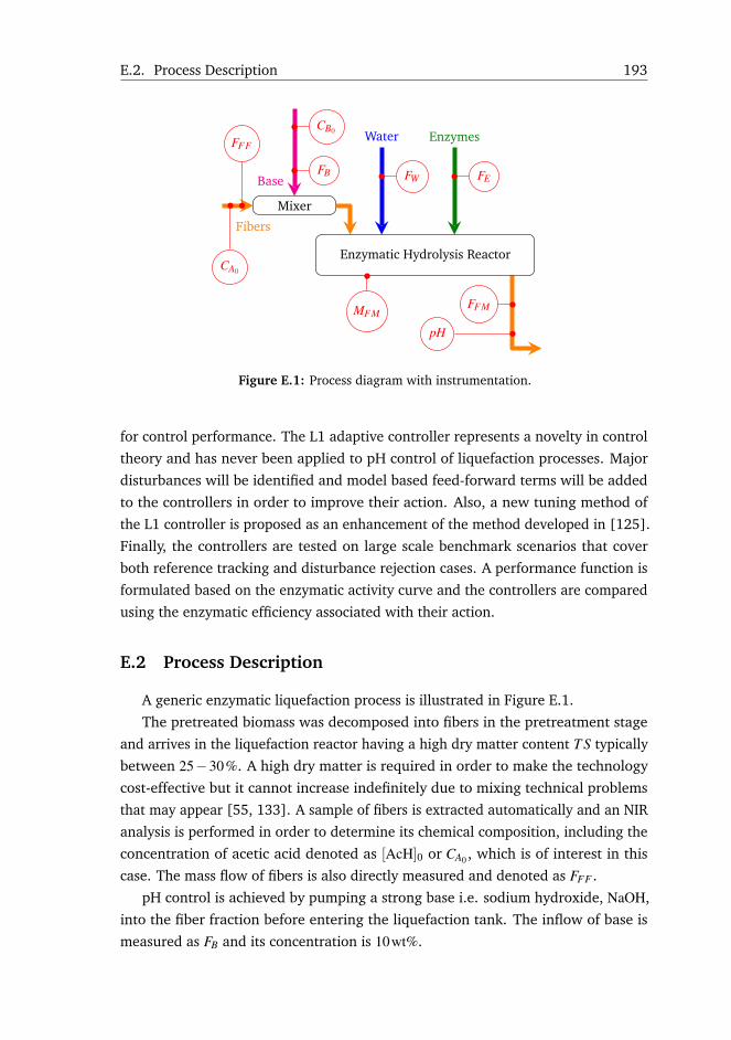
E.2. Process Description 193
Mixer
Fibers
Base
Water Enzymes
Enzymatic Hydrolysis Reactor
FFF
CA0
CB0
FB FW FE
FFM
pH
MFM
Figure E.1: Process diagram with instrumentation.
for control performance. The L1 adaptive controller represents a novelty in control
theory and has never been applied to pH control of liquefaction processes. Major
disturbances will be identified and model based feed-forward terms will be added
to the controllers in order to improve their action. Also, a new tuning method of
the L1 controller is proposed as an enhancement of the method developed in [125].
Finally, the controllers are tested on large scale benchmark scenarios that cover
both reference tracking and disturbance rejection cases. A performance function is
formulated based on the enzymatic activity curve and the controllers are compared
using the enzymatic efficiency associated with their action.
E.2 Process Description
A generic enzymatic liquefaction process is illustrated in Figure E.1.
The pretreated biomass was decomposed into fibers in the pretreatment stage
and arrives in the liquefaction reactor having a high dry matter content T S typically
between 25−30%. A high dry matter is required in order to make the technology
cost-effective but it cannot increase indefinitely due to mixing technical problems
that may appear [55, 133]. A sample of fibers is extracted automatically and an NIR
analysis is performed in order to determine its chemical composition, including the
concentration of acetic acid denoted as [AcH]0 or CA0 , which is of interest in this
case. The mass flow of fibers is also directly measured and denoted as FFF .
pH control is achieved by pumping a strong base i.e. sodium hydroxide, NaOH,
into the fiber fraction before entering the liquefaction tank. The inflow of base is
measured as FB and its concentration is 10wt%.
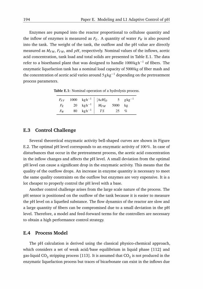
194 Paper E. Modeling and L1 Adaptive Control of pH
Enzymes are pumped into the reactor proportional to cellulose quantity and
the inflow of enzymes is measured as FE . A quantity of water FW is also poured
into the tank. The weight of the tank, the outflow and the pH value are directly
measured as MFM, FFM, and pH, respectively. Nominal values of the inflows, acetic
acid concentration, tank load and total solids are presented in Table E.1. The data
refer to a bioethanol plant that was designed to handle 1000kgh−1 of fibers. The
enzymatic liquefaction tank has a nominal load capacity of 5000kg of fiber mash and
the concentration of acetic acid varies around 5gkg−1 depending on the pretreatment
process parameters.
Table E.1: Nominal operation of a hydrolysis process.
FFF 1000 kgh−1 [AcH]0 5 gkg−1
FE 20 kgh−1 MFM 5000 kg
FW 80 kgh−1 T S 25 %
E.3 Control Challenge
Several theoretical enzymatic activity bell-shaped curves are shown in Figure
E.2. The optimal pH level corresponds to an enzymatic activity of 100%. In case of
disturbances that occur in the pretreatment process, the acetic acid concentration
in the inflow changes and affects the pH level. A small deviation from the optimal
pH level can cause a significant drop in the enzymatic activity. This means that the
quality of the outflow drops. An increase in enzyme quantity is necessary to meet
the same quality constraints on the outflow but enzymes are very expensive. It is a
lot cheaper to properly control the pH level with a base.
Another control challenge arises from the large scale nature of the process. The
pH sensor is positioned on the outflow of the tank because it is easier to measure
the pH level on a liquefied substance. The flow dynamics of the reactor are slow and
a large quantity of fibers can be compromised due to a small deviation in the pH
level. Therefore, a model and feed-forward terms for the controllers are necessary
to obtain a high performance control strategy.
E.4 Process Model
The pH calculation is derived using the classical physico-chemical approach,
which considers a set of weak acid/base equilibrium in liquid phase [112] and
gas-liquid CO2 stripping process [113]. It is assumed that CO2 is not produced in the
enzymatic liquefaction process but traces of bicarbonate can exist in the inflows due

E.4. Process Model 195
3 3.5 4 4.5 5 5.5 6
0
50
100
pH [−]
Enzy
mat
icA
ctiv
ity[%
]
Enzymatic Activity as a Function of pH
E1E2E3
Figure E.2: Different enzymatic activity bell-shaped curves.
to upstream subprocesses or process water utilization. The process model captures
flow dynamics and considers the mixture in chemical equilibrium at any given time.
E.4.1 pH Calculation
In total, the model has 6 weak acid/base equilibrium equations and CO2 stripping.
It is also assumed that production and consumption of ions are negligible from
enzymatic reactions.
Acetic acid is a weak acid and partially dissociates into Ac− and H+ with an equi-
librium constant KA (E.1a). Sodium hydroxide is a strong base and fully dissociates
into Na+ and OH− (E.1b). Ac− and Na+ combine to form the salt sodium acetate
NaAc (E.1c). Water self-ionizes with an equilibrium constant KW (E.1d). The liquid
phase is not pure and is considered to contain CO2, which is the cause of a buffer
formation that affects the pH level. Carbon dioxide forms carbonic acid H2CO3 in
water, which dissociates with an equilibrium constant KC1 into bicarbonate HCO −3
and H+ as in (E.1e). The bicarbonate continues to decompose forming carbonate
CO 2−3 and H+ with an equilibrium constant KC2 like in (E.1f).
AcH ↽−−−⇀ Ac−+H+ (E.1a)
NaOH−−→ Na++OH− (E.1b)
Ac−+Na+ −−→ NaAc (E.1c)
H++OH− ↽−−−⇀ H2O (E.1d)
CO2 +H2O−−→ H2CO3 ↽−−−⇀ HCO −3 +H+ (E.1e)
HCO −3 ↽−−−⇀ CO 2−
3 +H+ (E.1f)
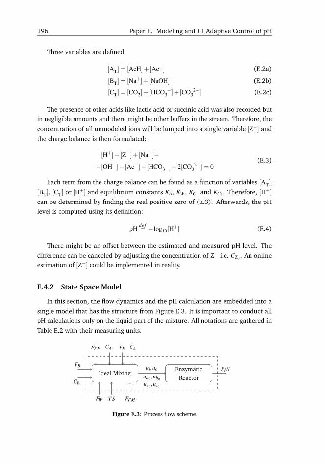
196 Paper E. Modeling and L1 Adaptive Control of pH
Three variables are defined:
[AT] = [AcH]+ [Ac−] (E.2a)
[BT] = [Na+]+ [NaOH] (E.2b)
[CT] = [CO2]+ [HCO −3 ]+ [CO 2−
3 ] (E.2c)
The presence of other acids like lactic acid or succinic acid was also recorded but
in negligible amounts and there might be other buffers in the stream. Therefore, the
concentration of all unmodeled ions will be lumped into a single variable [Z−] and
the charge balance is then formulated:
[H+]− [Z−]+ [Na+]−−[OH−]− [Ac−]− [HCO −
3 ]−2[CO 2−3 ] = 0
(E.3)
Each term from the charge balance can be found as a function of variables [AT],
[BT], [CT] or [H+] and equilibrium constants KA, KW , KC1 and KC2 . Therefore, [H+]
can be determined by finding the real positive zero of (E.3). Afterwards, the pH
level is computed using its definition:
pHde f= − log10[H
+] (E.4)
There might be an offset between the estimated and measured pH level. The
difference can be canceled by adjusting the concentration of Z– i.e. CZ0 . An online
estimation of [Z−] could be implemented in reality.
E.4.2 State Space Model
In this section, the flow dynamics and the pH calculation are embedded into a
single model that has the structure from Figure E.3. It is important to conduct all
pH calculations only on the liquid part of the mixture. All notations are gathered in
Table E.2 with their measuring units.
Ideal MixingEnzymatic
Reactor
FB
CB0
FFF CA0 FE CZ0
FW T S FFM
ui,uo
ua0 ,ub0
uc0 ,uz0
ypH
Figure E.3: Process flow scheme.
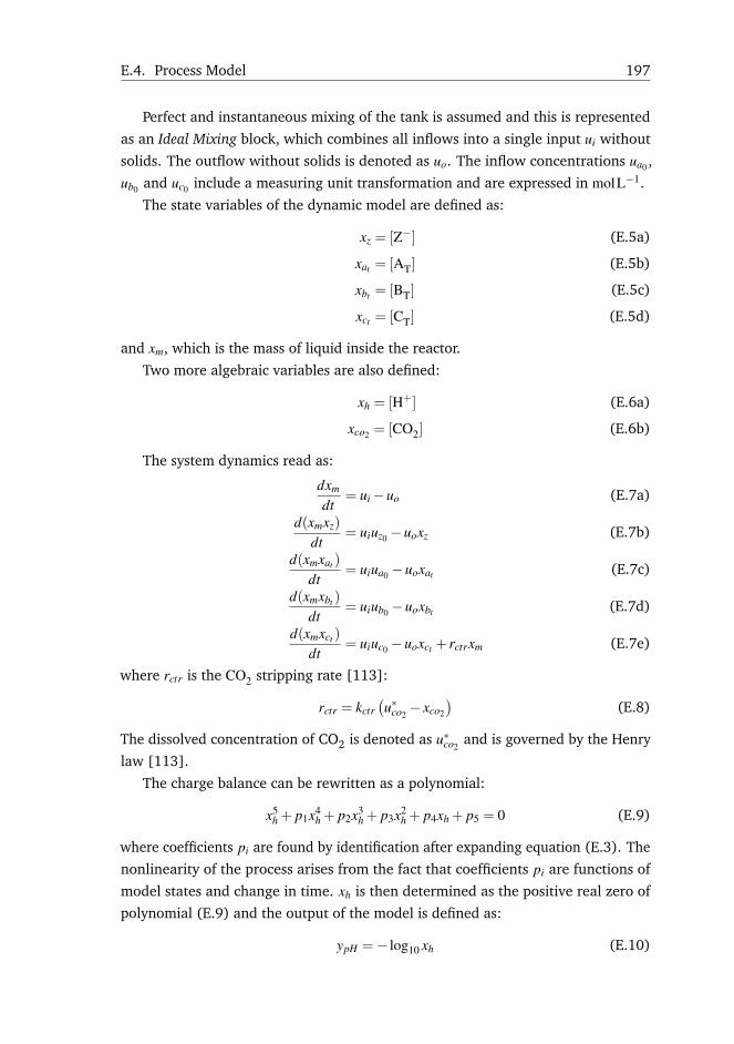
E.4. Process Model 197
Perfect and instantaneous mixing of the tank is assumed and this is represented
as an Ideal Mixing block, which combines all inflows into a single input ui without
solids. The outflow without solids is denoted as uo. The inflow concentrations ua0 ,
ub0 and uc0 include a measuring unit transformation and are expressed in molL−1.
The state variables of the dynamic model are defined as:
xz = [Z−] (E.5a)
xat = [AT] (E.5b)
xbt = [BT] (E.5c)
xct = [CT] (E.5d)
and xm, which is the mass of liquid inside the reactor.
Two more algebraic variables are also defined:
xh = [H+] (E.6a)
xco2 = [CO2] (E.6b)
The system dynamics read as:
dxm
dt= ui−uo (E.7a)
d(xmxz)
dt= uiuz0 −uoxz (E.7b)
d(xmxat )
dt= uiua0 −uoxat (E.7c)
d(xmxbt )
dt= uiub0 −uoxbt (E.7d)
d(xmxct )
dt= uiuc0 −uoxct + rctrxm (E.7e)
where rctr is the CO2 stripping rate [113]:
rctr = kctr(u∗co2− xco2
)(E.8)
The dissolved concentration of CO2 is denoted as u∗co2and is governed by the Henry
law [113].
The charge balance can be rewritten as a polynomial:
x5h + p1x4
h + p2x3h + p3x2
h + p4xh + p5 = 0 (E.9)
where coefficients pi are found by identification after expanding equation (E.3). The
nonlinearity of the process arises from the fact that coefficients pi are functions of
model states and change in time. xh is then determined as the positive real zero of
polynomial (E.9) and the output of the model is defined as:
ypH =− log10 xh (E.10)
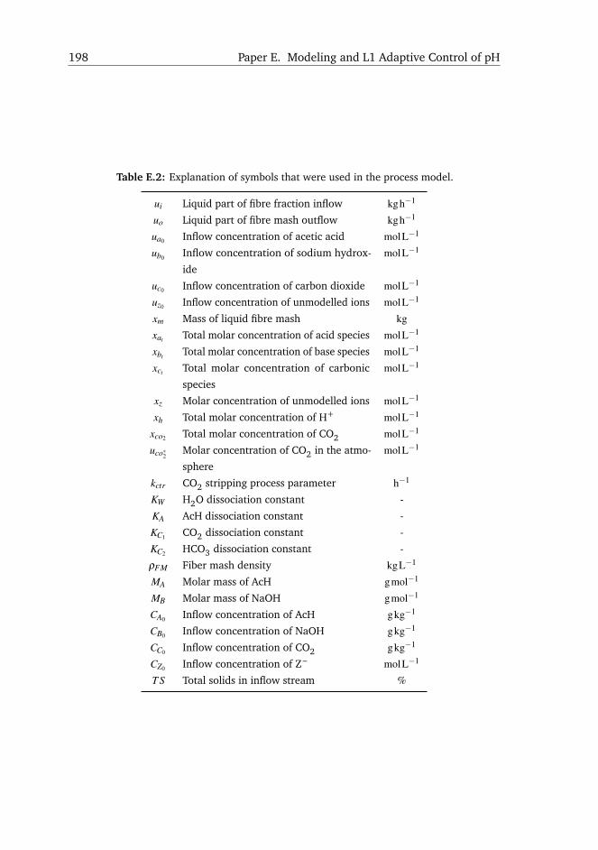
198 Paper E. Modeling and L1 Adaptive Control of pH
Table E.2: Explanation of symbols that were used in the process model.
ui Liquid part of fibre fraction inflow kgh−1
uo Liquid part of fibre mash outflow kgh−1
ua0 Inflow concentration of acetic acid molL−1
ub0 Inflow concentration of sodium hydrox-
ide
molL−1
uc0 Inflow concentration of carbon dioxide molL−1
uz0 Inflow concentration of unmodelled ions molL−1
xm Mass of liquid fibre mash kg
xat Total molar concentration of acid species molL−1
xbt Total molar concentration of base species molL−1
xct Total molar concentration of carbonic
species
molL−1
xz Molar concentration of unmodelled ions molL−1
xh Total molar concentration of H+ molL−1
xco2 Total molar concentration of CO2 molL−1
uco∗2 Molar concentration of CO2 in the atmo-
sphere
molL−1
kctr CO2 stripping process parameter h−1
KW H2O dissociation constant -
KA AcH dissociation constant -
KC1 CO2 dissociation constant -
KC2 HCO3 dissociation constant -
ρFM Fiber mash density kgL−1
MA Molar mass of AcH gmol−1
MB Molar mass of NaOH gmol−1
CA0 Inflow concentration of AcH gkg−1
CB0 Inflow concentration of NaOH gkg−1
CC0 Inflow concentration of CO2 gkg−1
CZ0 Inflow concentration of Z– molL−1
T S Total solids in inflow stream %

E.4. Process Model 199
The numerical values of all model parameters are listed in Table E.3.
Table E.3: Model parameters.
KW 1×10⁻¹⁴ MA 60.05221 gmol−1
KA 1.7378×10−5 MB 39.99715 gmol−1
KC1 4.3003×10⁻⁷ MC 44.01 gmol−1
KC2 4.7995×10⁻¹¹ CA0 5 gkg−1
u∗co21.71×10−5 molL−1 CB0 100 gkg−1
ρFM 1.05 kgL−1 CC0 7.1673×10⁻⁴ gkg−1
CZ0 0.08molL−1
E.4.3 Titration Simulation
The model is tested by performing a classical titration simulation, i.e. feeding
into the process an inflow of hydroxide resembling a stairway shape with a stair
amplitude of 1kgh−1 starting at time 20h. The concentration of Z− is disregarded.
The results can be observed in Figure E.4.
0
0.05
0.1
0.15
C[m
olL−
1 ]
Concentration of Species and pH
CAT
CBT
CCT
0 200 400 600 800 1000
5
10
Time [h]
pH[−
]
Figure E.4: Titration simulation for verifying the implementation of the model.
The acetic acid and the carbonic acid keep a low pH but after adding a substantial
amount of base, approximately at time t = 500h, the buffers are depleted and the
pH increases to a value greater than 7, which is an expected result.
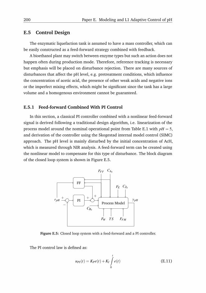
200 Paper E. Modeling and L1 Adaptive Control of pH
E.5 Control Design
The enzymatic liquefaction tank is assumed to have a mass controller, which can
be easily constructed as a feed-forward strategy combined with feedback.
A bioethanol plant may switch between enzyme types but such an action does not
happen often during production mode. Therefore, reference tracking is necessary
but emphasis will be placed on disturbance rejection. There are many sources of
disturbances that affect the pH level, e.g. pretreatment conditions, which influence
the concentration of acetic acid, the presence of other weak acids and negative ions
or the imperfect mixing effects, which might be significant since the tank has a large
volume and a homogenous environment cannot be guaranteed.
E.5.1 Feed-forward Combined With PI Control
In this section, a classical PI controller combined with a nonlinear feed-forward
signal is derived following a traditional design algorithm, i.e. linearization of the
process model around the nominal operational point from Table E.1 with pH = 5,
and derivation of the controller using the Skogestad internal model control (SIMC)
approach. The pH level is mainly disturbed by the initial concentration of AcH,
which is measured through NIR analysis. A feed-forward term can be created using
the nonlinear model to compensate for this type of disturbance. The block diagram
of the closed loop system is shown in Figure E.5.
Process ModelCB0
FFF CA0
FE CZ0
FW T S FFM
PI+
FF
+ypH
−rpH
+
Figure E.5: Closed loop system with a feed-forward and a PI controller.
The PI control law is defined as:
uPI(t) = KPe(t)+KI
t∫0
e(t) (E.11)
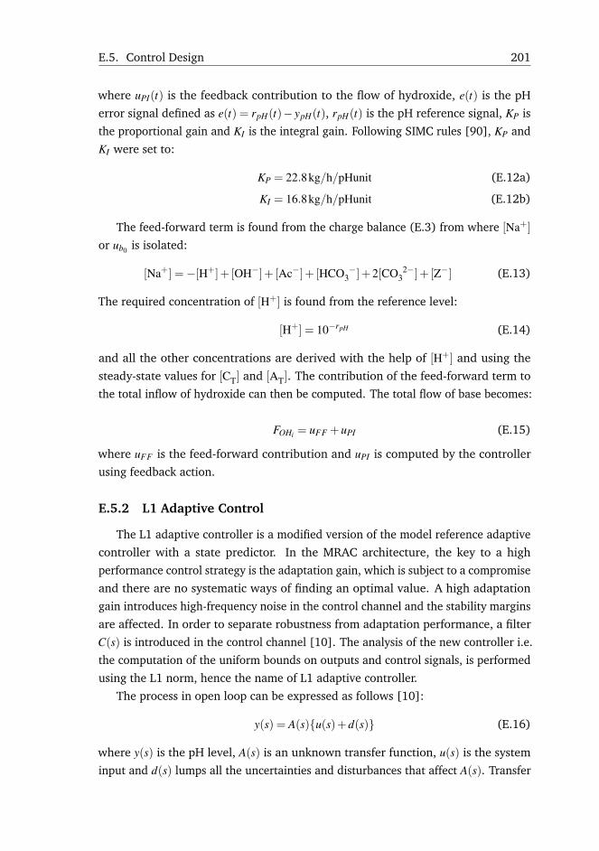
E.5. Control Design 201
where uPI(t) is the feedback contribution to the flow of hydroxide, e(t) is the pH
error signal defined as e(t) = rpH(t)− ypH(t), rpH(t) is the pH reference signal, KP is
the proportional gain and KI is the integral gain. Following SIMC rules [90], KP and
KI were set to:
KP = 22.8kg/h/pHunit (E.12a)
KI = 16.8kg/h/pHunit (E.12b)
The feed-forward term is found from the charge balance (E.3) from where [Na+]or ub0 is isolated:
[Na+] =−[H+]+ [OH−]+ [Ac−]+ [HCO −3 ]+2[CO 2−
3 ]+ [Z−] (E.13)
The required concentration of [H+] is found from the reference level:
[H+] = 10−rpH (E.14)
and all the other concentrations are derived with the help of [H+] and using the
steady-state values for [CT] and [AT]. The contribution of the feed-forward term to
the total inflow of hydroxide can then be computed. The total flow of base becomes:
FOHi = uFF +uPI (E.15)
where uFF is the feed-forward contribution and uPI is computed by the controller
using feedback action.
E.5.2 L1 Adaptive Control
The L1 adaptive controller is a modified version of the model reference adaptive
controller with a state predictor. In the MRAC architecture, the key to a high
performance control strategy is the adaptation gain, which is subject to a compromise
and there are no systematic ways of finding an optimal value. A high adaptation
gain introduces high-frequency noise in the control channel and the stability margins
are affected. In order to separate robustness from adaptation performance, a filter
C(s) is introduced in the control channel [10]. The analysis of the new controller i.e.
the computation of the uniform bounds on outputs and control signals, is performed
using the L1 norm, hence the name of L1 adaptive controller.
The process in open loop can be expressed as follows [10]:
y(s) = A(s){u(s)+d(s)} (E.16)
where y(s) is the pH level, A(s) is an unknown transfer function, u(s) is the system
input and d(s) lumps all the uncertainties and disturbances that affect A(s). Transfer
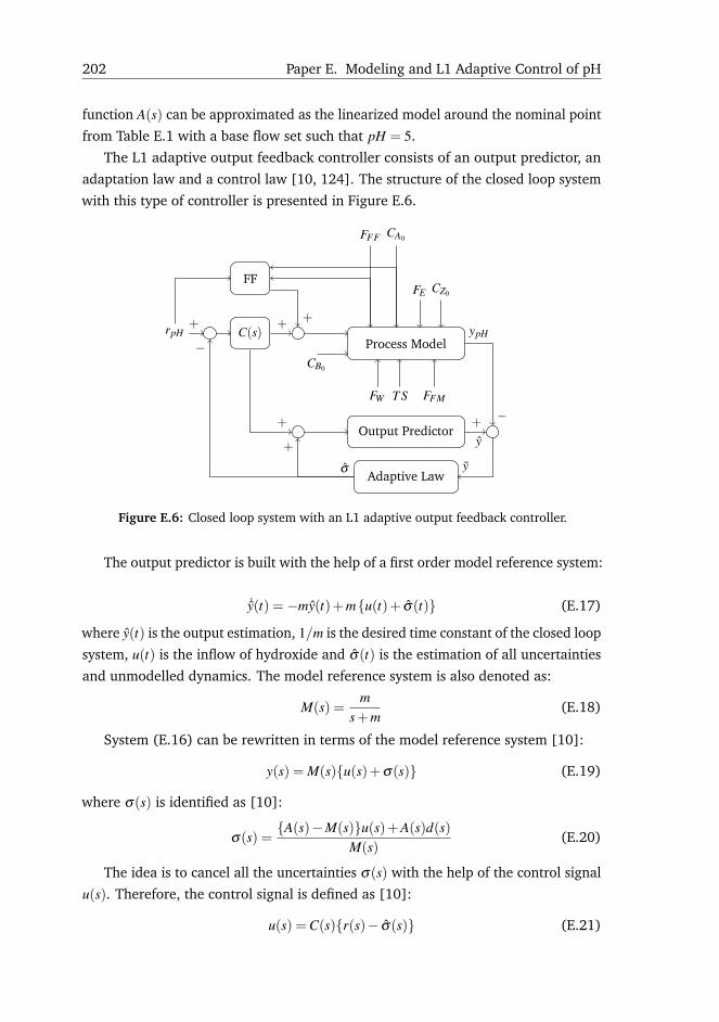
202 Paper E. Modeling and L1 Adaptive Control of pH
function A(s) can be approximated as the linearized model around the nominal point
from Table E.1 with a base flow set such that pH = 5.
The L1 adaptive output feedback controller consists of an output predictor, an
adaptation law and a control law [10, 124]. The structure of the closed loop system
with this type of controller is presented in Figure E.6.
Process ModelCB0
FFF CA0
FE CZ0
FW T S FFM
C(s)+
FF
+rpH
+
Output Predictor
Adaptive Law
ypH
−+
y
y
+
σ
+
−
Figure E.6: Closed loop system with an L1 adaptive output feedback controller.
The output predictor is built with the help of a first order model reference system:
˙y(t) =−my(t)+m{u(t)+ σ(t)} (E.17)
where y(t) is the output estimation, 1/m is the desired time constant of the closed loop
system, u(t) is the inflow of hydroxide and σ(t) is the estimation of all uncertainties
and unmodelled dynamics. The model reference system is also denoted as:
M(s) =m
s+m(E.18)
System (E.16) can be rewritten in terms of the model reference system [10]:
y(s) = M(s){u(s)+σ(s)} (E.19)
where σ(s) is identified as [10]:
σ(s) ={A(s)−M(s)}u(s)+A(s)d(s)
M(s)(E.20)
The idea is to cancel all the uncertainties σ(s) with the help of the control signal
u(s). Therefore, the control signal is defined as [10]:
u(s) =C(s){r(s)− σ(s)} (E.21)

E.5. Control Design 203
where C(s) is a first order filter in this application:
C(s) =c
s+ c(E.22)
If Equation (E.21) is substituted in (E.19) then:
y(s) = M(s)C(s)r(s)+M(s){σ(s)−C(s)σ(s)} (E.23)
If σ(s) is perfectly estimated then σ(s) = σ(s) and the disturbances will be rejected
only in the bandwidth of C(s).
The adaptive estimate σ(t) is updated using a projection algorithm that ensures
boundedness of the estimate within a given ball [10]:
˙σ(t) = ΓProj(σ(t),−y(t)) (E.24)
where y(t) = y(t)− y(t) is the estimation error of the output.
There are 3 parameters to set for the L1 adaptive output feedback controller,
i.e. the desired closed loop time constant 1/m, the adaptation gain Γ and the
eigenfrequency of the control filter c.
The reference model and the control signal filter can be designed systematically
[125]. Assuming perfect knowledge of disturbances, an ideal system y(s) can be
built and used for tuning [125]:
y(s) = H(s)C(s)r(s)+H(s){1−C(s)}d(s) (E.25)
where H(s)C(s) is the transfer function from r(s) to y(s) and H(s) is defined as:
H(s) =A(s)M(s)
C(s)A(s)+{1−C(s)}M(s)(E.26)
Parameters m and c must be chosen such that H(s) is stable and the following L1
norm holds [10]:
||G(s)||L1L < 1 (E.27)
where G(s) = H(s){1−C(s)} is the transfer function from d(s) to y(s) and L is the
Lipschitz constant required to guarantee BIBO stability (Lemma 4.1.1 in [10]).
By considering A(s) as the linearized system around the nominal point, a (m,c)
map can be built in order to facilitate the choice of these two parameters. The closed
loop system has several poles, which can cause oscillations if they are complex. As a
criterion for (m,c) determination, the worst damping ratio ζ should be higher than
0.7 in order to ensure acceptable oscillations. The damping ratio ζ is plotted as a
function of (m,c) in the top plot of Figure E.7.
In order to accelerate the system, parameter m should be increased. To reduce
oscillations in the system response, the bandwidth of filter C(s) needs to be enlarged

204 Paper E. Modeling and L1 Adaptive Control of pH
0.2 0.3 0.4 0.5 0.6 0.7 0.8 0.9
50
100
m [rads−1]
c[r
ads−
1 ]Choice of m and c
0.6
0.8
1.0
ζ
0 1000 2000 3000 4000 5000
0.4
0.6
0.8
1
Γ [−]
ζ Γ[−
]
Choice of Γ
Figure E.7: Tuning of the L1 adaptive controller.
such that a more responsive control action would be allowed. The pair (0.6,60) is
chosen for this application, which corresponds to a ζ > 0.9:
m = 0.6 c = 60 (E.28)
The model reference has a time constant that corresponds to 1.6h. The Lipschitz
constant, for the selected m and c, is computed to be:
L = 78.6851 (E.29)
which ensures a BIBO closed loop system according to Lemma 4.1.1 [10].
In theorem 4.1.1 from [10] it is shown that the tracking error between the
real and the ideal system, which assumes perfect knowledge of the disturbance, is
uniformly bounded with respect to a constant proportional to 1/√
Γ. Therefore, a
high adaptation gain Γ is desired. At the same time, the stability and dynamics of σare dependent on Γ. The transfer function from r(s) and d(s) to σ(s) is [125]:
σ = F(s)[C(s){A(s)−M(s)}r(s)+A(s)d(s)] (E.30)
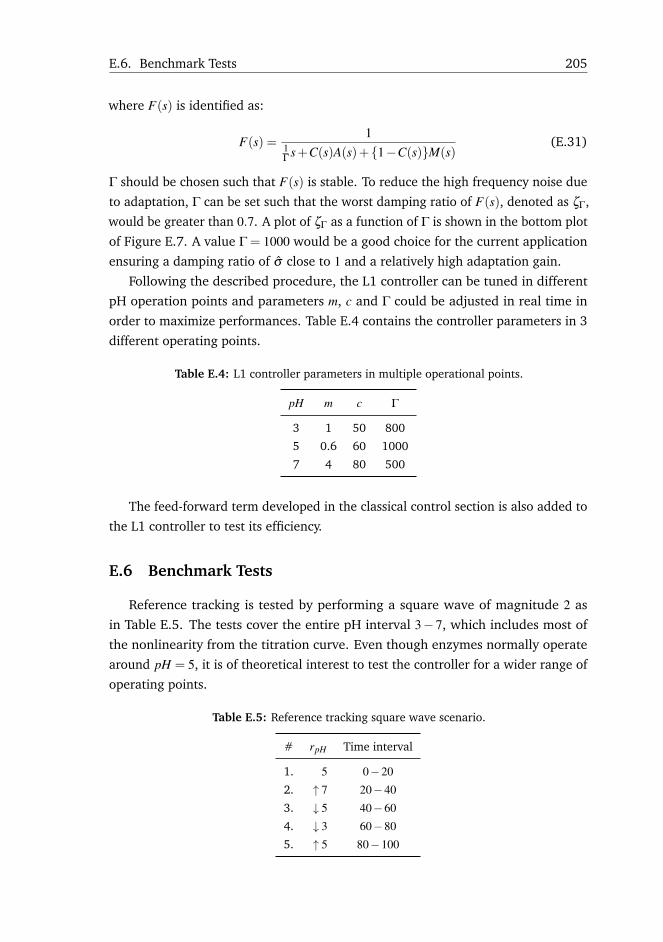
E.6. Benchmark Tests 205
where F(s) is identified as:
F(s) =1
1Γ s+C(s)A(s)+{1−C(s)}M(s)
(E.31)
Γ should be chosen such that F(s) is stable. To reduce the high frequency noise due
to adaptation, Γ can be set such that the worst damping ratio of F(s), denoted as ζΓ,
would be greater than 0.7. A plot of ζΓ as a function of Γ is shown in the bottom plot
of Figure E.7. A value Γ = 1000 would be a good choice for the current application
ensuring a damping ratio of σ close to 1 and a relatively high adaptation gain.
Following the described procedure, the L1 controller can be tuned in different
pH operation points and parameters m, c and Γ could be adjusted in real time in
order to maximize performances. Table E.4 contains the controller parameters in 3
different operating points.
Table E.4: L1 controller parameters in multiple operational points.
pH m c Γ
3 1 50 800
5 0.6 60 1000
7 4 80 500
The feed-forward term developed in the classical control section is also added to
the L1 controller to test its efficiency.
E.6 Benchmark Tests
Reference tracking is tested by performing a square wave of magnitude 2 as
in Table E.5. The tests cover the entire pH interval 3− 7, which includes most of
the nonlinearity from the titration curve. Even though enzymes normally operate
around pH = 5, it is of theoretical interest to test the controller for a wider range of
operating points.
Table E.5: Reference tracking square wave scenario.
# rpH Time interval
1. 5 0−20
2. ↑ 7 20−40
3. ↓ 5 40−60
4. ↓ 3 60−80
5. ↑ 5 80−100
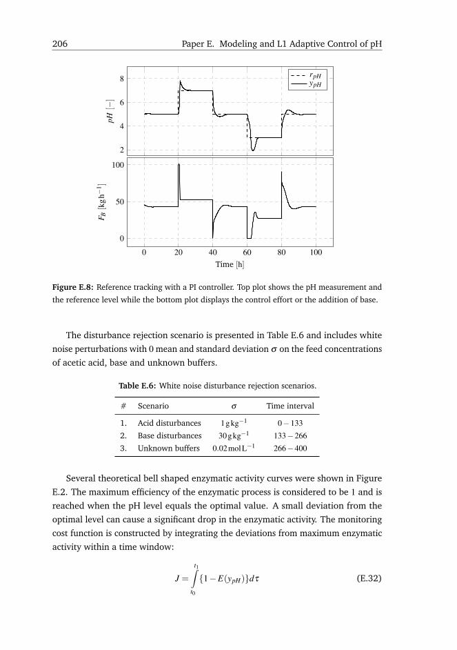
206 Paper E. Modeling and L1 Adaptive Control of pH
2
4
6
8
pH[−
]
rpHypH
0 20 40 60 80 100
0
50
100
Time [h]
F B[k
gh−
1 ]
Figure E.8: Reference tracking with a PI controller. Top plot shows the pH measurement and
the reference level while the bottom plot displays the control effort or the addition of base.
The disturbance rejection scenario is presented in Table E.6 and includes white
noise perturbations with 0 mean and standard deviation σ on the feed concentrations
of acetic acid, base and unknown buffers.
Table E.6: White noise disturbance rejection scenarios.
# Scenario σ Time interval
1. Acid disturbances 1gkg−1 0−133
2. Base disturbances 30gkg−1 133−266
3. Unknown buffers 0.02molL−1 266−400
Several theoretical bell shaped enzymatic activity curves were shown in Figure
E.2. The maximum efficiency of the enzymatic process is considered to be 1 and is
reached when the pH level equals the optimal value. A small deviation from the
optimal level can cause a significant drop in the enzymatic activity. The monitoring
cost function is constructed by integrating the deviations from maximum enzymatic
activity within a time window:
J =
t1∫t0
{1−E(ypH)}dτ (E.32)
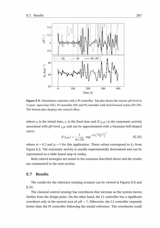
E.7. Results 207
4.8
5
5.2
5.4
Acid Dis-
turbance
Base Dis-
turbance
Z Distur-
bance
pH[−
]
0 100 200 300 40020
40
60
Time [h]
F B[k
gh−
1 ]
OL PI PI+FF
Figure E.9: Disturbance rejection with a PI controller. Top plot shows the reactor pH level in
3 cases: open loop (OL), PI controller (PI) and PI controller with feed-forward action (PI+FF).
The bottom plot displays the control effort.
where t0 is the initial time, t1 is the final time and E(ypH) is the enzymatic activity
associated with pH level ypH and can be approximated with a Gaussian bell-shaped
curve:
E(ypH) =1
σ√
2π· exp−0.5
( ypH−µσ
)2
(E.33)
where σ = 0.2 and µ = 5 for this application. These values correspond to E2 from
Figure E.2. The enzymatic activity is usually experimentally determined and can be
represented as a table based map in reality.
Both control strategies are tested in the scenarios described above and the results
are commented in the next section.
E.7 Results
The results for the reference tracking scenario can be viewed in Figures E.8 and
E.10.
The classical control strategy has overshoots that increase as the system moves
further from the design point. On the other hand, the L1 controller has a significant
overshoot only in the neutral area of pH = 7. Otherwise, the L1 controller responds
better than the PI controller following the model reference. The overshoots could

208 Paper E. Modeling and L1 Adaptive Control of pH
2
4
6
8
pH[−
]
rpHypH
0 20 40 60 80 100
0
50
100
Time [h]
F B[k
gh−
1 ]
Figure E.10: Reference tracking with an L1 controller. Top plot shows the pH measurement
and the reference level while the bottom plot displays the control effort or the addition of
base.
be accommodated by a reference filter in both cases. The control signal is within
acceptable limits.
The disturbance rejection scenario is shown in Figures E.9 and E.11 and the
evaluation of the cost function is performed in Table E.7. In the case of measured
disturbances, i.e. acetic acid disturbances, the L1 controller with feed-forward
performs better than the PI controller leading to a full rejection of these disturbances.
The nonlinear feed-forward term significantly helps both controllers.
In the second scenario, i.e. base disturbances, the L1 controller has better results
leading to smaller variations of the pH level, thus to a much lower J value. The
feed-forward term does not help in this case.
In the last scenario, i.e. unknown buffers, the L1 controller outperforms the
classical PI. Overall, regarding variations in the pH level, the L1 controller has better
performances.
E.8 Conclusions
In this article, for the first time to our knowledge, a pH model of the enzymatic
liquefaction process has been developed. Reference tracking and disturbance rejec-
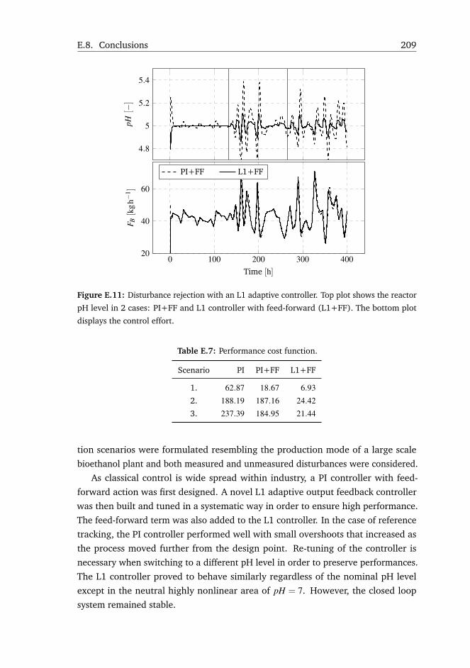
E.8. Conclusions 209
4.8
5
5.2
5.4
Acid Dis-
turbance
Base Dis-
turbance
Z Distur-
bance
pH[−
]
0 100 200 300 40020
40
60
Time [h]
F B[k
gh−
1 ]
PI+FF L1+FF
Figure E.11: Disturbance rejection with an L1 adaptive controller. Top plot shows the reactor
pH level in 2 cases: PI+FF and L1 controller with feed-forward (L1+FF). The bottom plot
displays the control effort.
Table E.7: Performance cost function.
Scenario PI PI+FF L1+FF
1. 62.87 18.67 6.93
2. 188.19 187.16 24.42
3. 237.39 184.95 21.44
tion scenarios were formulated resembling the production mode of a large scale
bioethanol plant and both measured and unmeasured disturbances were considered.
As classical control is wide spread within industry, a PI controller with feed-
forward action was first designed. A novel L1 adaptive output feedback controller
was then built and tuned in a systematic way in order to ensure high performance.
The feed-forward term was also added to the L1 controller. In the case of reference
tracking, the PI controller performed well with small overshoots that increased as
the process moved further from the design point. Re-tuning of the controller is
necessary when switching to a different pH level in order to preserve performances.
The L1 controller proved to behave similarly regardless of the nominal pH level
except in the neutral highly nonlinear area of pH = 7. However, the closed loop
system remained stable.
210 Paper E. Modeling and L1 Adaptive Control of pH
In the case of measured disturbances, both control strategies were effective
and it was shown that the feed-forward term considerably improves the system
response. In the case of unmeasured disturbances, the L1 adaptive controller had
better performances.
A new cost function was derived from the enzymatic bell-shaped activity curve
to assess closed loop performances. This cost function was further used to monitor
the efficiency of the enzymatic process.
Finally, a tuning method was proposed for the L1 controller that proved to be
very effective for this application. This tuning procedure is an enhancement of the
method presented in [125].
Acknowledgements
The close collaboration and very helpful suggestions and detailed comments
received from Dr. Jakob M. Jensen on this research are gratefully acknowledged.
Bibliography
[1] R. Datta, M. A. Maher, C. Jones, and R. W. Brinker. “Ethanol-the primary
renewable liquid fuel”. Journal of Chemical Technology and Biotechnology 86
(2011), pp. 473–480. DOI: 10.1002/jctb.2580.
[2] R. C. Brown, T. Brown, S. Capareda, B. Dale, D. Edwards, V. Estes, C.
Granda, M. Holtzapple, S. Lonkar, and C. E. Wyman. “SBE Supplement:
Lignocellulosic Biofuels”. AIChE CEP (2015), pp. 33–64.
[3] J. Larsen, M. Ø. Haven, and L. Thirup. “Inbicon makes lignocellulosic ethanol
a commercial reality”. Biomass and Bioenergy 46 (Nov. 2012), pp. 36–45.
DOI: 10.1016/j.biombioe.2012.03.033.
[4] J. Larsen, M. Ø. Petersen, L. Thirup, H. W. Li, and F. K. Iversen. “The IBUS
Process - Lignocellulosic Bioethanol Close to a Commercial Reality”. ChemicalEngineering & Technology 31 (May 2008), pp. 765–772. DOI: 10.1002/ceat.
200800048.
[5] R. M. Prunescu, M. Blanke, J. G. Jakobsen, and G. Sin. “Dynamic modeling
and validation of a biomass hydrothermal pretreatment process - A demon-
stration scale study”. AIChE Journal (2015). DOI: 10.1002/aic.14954.
[6] R. M. Prunescu and G. Sin. “Dynamic modeling and validation of a lig-
nocellulosic enzymatic hydrolysis process - A demonstration scale study”.
Bioresource Technology 150 (Dec. 2013), pp. 393–403. DOI: 10.1016/j.
biortech.2013.10.029.
[7] R. M. Prunescu, M. Blanke, J. G. Jakobsen, and G. Sin. “Model-Based
Plantwide Optimization of a Large Scale Lignocellulosic Bioethanol Plant”.
Submitted to AIChE Journal (2015).
[8] G. Sin, A. S. Meyer, and K. V. Gernaey. “Assessing reliability of cellulose
hydrolysis models to support biofuel process design - Identifiability and
uncertainty analysis”. Computers & Chemical Engineering 34 (Sept. 2010),
pp. 1385–1392. DOI: 10.1016/j.compchemeng.2010.02.012.
212 Bibliography
[9] R. Morales-Rodriguez, A. S. Meyer, K. V. Gernaey, and G. Sin. “A framework
for model-based optimization of bioprocesses under uncertainty: Lignocellu-
losic ethanol production case”. Computers & Chemical Engineering 42 (July
2012), pp. 115–129. DOI: 10.1016/j.compchemeng.2011.12.004.
[10] N. Hovakimyan and C. Cao. L1 Adaptive Control Theory. SIAM, 2010.
[11] R. M. Prunescu, M. Blanke, and G. Sin. “Modelling and L1 Adaptive Control
of pH in Bioethanol Enzymatic Process”. Proceedings of the 2013 AmericanControl Conference. Washington D.C., USA, 2013, pp. 1888–1895.
[12] R. M. Prunescu, M. Blanke, and G. Sin. “Modelling and L1 Adaptive Control
of Temperature in Biomass Pretreatment”. Proceedings of the 52nd IEEEConference on Decision and Control. Florence, Italy, 2013, pp. 3152–3159.
[13] J. Conti, P. Holtberg, J. A. Beamon, S. Napolitano, M. A. Schaal, J. T. Turnure,
and L. Westfall. International Energy Outlook 2013. Tech. rep. 2013. DOI:
EIA-0484(2013).
[14] R. Guseo, A. Dalla Valle, and M. Guidolin. “World Oil Depletion Models: Price
effects compared with strategic or technological interventions”. TechnologicalForecasting and Social Change 74.4 (2007), pp. 452–469. DOI: 10.1016/j.
techfore.2006.01.004.
[15] K. Mohaddes. “Econometric Modelling of World Oil Supplies: Terminal Price
and the Time to Depletion”. OPEC Energy Review (2012), pp. 162–193.
[16] C. McGlade and P. Ekins. “The geographical distribution of fossil fuels unused
when limiting global warming to 2C”. Nature 517.7533 (2014), pp. 187–190.
DOI: 10.1038/nature14016.
[17] T. Gasser, C. Guivarch, K. Tachiiri, C. D. Jones, and P. Ciais. “Negative
emissions physically needed to keep global warming below 2C”. NatureCommunications 6 (2015), p. 7958. DOI: 10.1038/ncomms8958.
[18] N. Armaroli and V. Balzani. “The legacy of fossil fuels”. Chemistry - An AsianJournal 6.3 (2011), pp. 768–784. DOI: 10.1002/asia.201000797.
[19] United Nations. Kyoto Protocol To the United Nations Framework. 1998. DOI:
10.1111/1467-9388.00150.
[20] M. Wang, M. Wu, and H. Huo. “Life-cycle energy and greenhouse gas emis-
sion impacts of different corn ethanol plant types”. Environmental ResearchLetters 2.2 (2007), pp. 1–13. DOI: 10.1088/1748-9326/2/2/024001.
[21] M. A. Martin. “First generation biofuels compete”. New Biotechnology 27.5
(2010), pp. 596–608. DOI: 10.1016/j.nbt.2010.06.010.
Bibliography 213
[22] Novozymes A/S. “Beta Renewables opens biofuels plant in Italy”. Focus onCatalysts (2013), p. 6. DOI: 10.1016/S1351-4180(13)70461-6.
[23] G. Dragone, B. Fernandes, A. Vicente, and J. Teixeira. “Third generation
biofuels from microalgae”. Current Research, Technology and Education Topicsin Applied Microbiology and Microbial Biotechnology (2010), pp. 1355–1366.
[24] F. Alam, S. Mobin, and H. Chowdhury. “Third Generation Biofuel from
Algae”. Procedia Engineering 105 (2015), pp. 763–768. DOI: 10.1016/j.
proeng.2015.05.068.
[25] J. Miranowski and A. Rosburg. “Long-term biofuel projections under different
oil price scenarios”. AgBioForum 16.1 (2013), pp. 79–87.
[26] P. Cheali, J. A. Posada, K. V. Gernaey, and G. Sin. “Upgrading of lignocel-
lulosic biorefinery to value-added chemicals: Sustainability and economics
of bioethanol-derivatives”. Biomass and Bioenergy 75 (2015), pp. 282–300.
DOI: 10.1016/j.biombioe.2015.02.030.
[27] C. E. Wyman and A. J. Ragauskas. “Lignin Bioproducts to Enable Biofuels”.
Biofuels, Bioproducts and Biorefining 9.5 (2015), pp. 447–449. DOI: 10.1002/
bbb.1582.
[28] A. J. Ragauskas, G. T. Beckham, M. J. Biddy, R. Chandra, F. Chen, M. F.
Davis, B. H. Davison, R. a. Dixon, P. Gilna, M. Keller, P. Langan, A. K. Naskar,
J. N. Saddler, T. J. Tschaplinski, G. a. Tuskan, and C. E. Wyman. “Lignin
valorization: improving lignin processing in the biorefinery.” Science (NewYork, N.Y.) 344.6185 (2014), p. 1246843. DOI: 10.1126/science.1246843.
[29] Innovation Fund Denmark. Innovation Fund Denmark 2015 Strategy. Tech.
rep. 2015.
[30] D. A. Mitchell, N. Krieger, and M. Berovic. Solid-State Fermentation Bioreac-tors. Springer, 2006. DOI: 10.1007/3540312854.
[31] N. Silver. The Signal and the Noise: The Art and Science of Prediction. Allen
Lane, 2012.
[32] R. M. Prunescu, M. Blanke, J. G. Jakobsen, and G. Sin. “Dynamic Modeling,
Advanced Control, Diagnosis and Optimization of Large-Scale Lignocellulosic
Biorefineries”. Proceedings of the AIChE 2015 Annual Meeting. Salt Lake City,
UT, USA, 2015.
[33] R. M. Prunescu, M. Blanke, J. G. Jakobsen, and G. Sin. “Plantwide Model-
Based Optimization of a Large Scale Second Generation Biorefinery”. Pro-ceedings of the AIChE 2015 Annual Meeting. Salt Lake City, UT, USA, 2015.
214 Bibliography
[34] R. M. Prunescu, M. Blanke, J. G. Jakobsen, and G. Sin. “Model-Based Filtering
of Large-Scale Datasets - A Biorefinery Application”. Proceedings of the AIChE2014 Annual Meeting. Atlanta, GA, USA, 2014.
[35] R. M. Prunescu and G. Sin. “Dynamic Simulation, Sensitivity and Uncertainty
Analysis of a Demonstration Scale Lignocellulosic Enzymatic Hydrolysis
Process”. Proceedings of the AIChE 2014 Annual Meeting. Atlanta, GA, USA,
2014.
[36] R. M. Prunescu, M. Blanke, and G. Sin. “Advances in Monitoring, Diagno-
sis and Control of Biorefineries”. Proceedings of the 9th World Congress ofChemical Engineering. Seoul, South Korea, 2013.
[37] A. Sluiter, B. Hames, R. Ruiz, C. Scarlata, J. Sluiter, D. Templeton, and D.
Crocker. “Determination of structural carbohydrates and lignin in biomass”.
Technical Report NREL/TP-510-42618 (2008). DOI: NREL/TP-510-42618.
[38] C. Carrasco, D. Cuno, K. Carlqvist, M. Galbe, and G. Lidén. “SO2-catalysed
steam pretreatment of quinoa stalks”. Journal of Chemical Technology &Biotechnology 90.1 (2015), pp. 64–71. DOI: 10.1002/jctb.4286.
[39] S. Collins, N. Wellner, I. Martinez Bordonado, A. L. Harper, C. N. Miller,
I. Bancroft, and K. W. Waldron. “Variation in the chemical composition of
wheat straw: the role of tissue ratio and composition”. Biotechnology forBiofuels 7.1 (2014), p. 121. DOI: 10.1186/PREACCEPT-4657379161257175.
[40] J. B. Kristensen, L. G. Thygesen, C. Felby, H. Jørgensen, and T. Elder. “Cell-
wall structural changes in wheat straw pretreated for bioethanol production.”
Biotechnology for biofuels 1 (Jan. 2008), pp. 1–9. DOI: 10.1186/1754-6834-
1-5.
[41] M. A. T. Hansen and J. B. Kristensen. “Pretreatment and enzymatic hydrolysis
of wheat straw (Triticum aestivum L.)–The impact of lignin relocation and
plant tissues on enzymatic accessibility”. Bioresource technology 102 (Feb.
2011), pp. 2804–2811. DOI: 10.1016/j.biortech.2010.10.030.
[42] N. D. Weiss, J. D. Farmer, and D. J. Schell. “Impact of corn stover composition
on hemicellulose conversion during dilute acid pretreatment and enzymatic
cellulose digestibility of the pretreated solids.” Bioresource technology 101
(Jan. 2010), pp. 674–678. DOI: 10.1016/j.biortech.2009.08.082.
[43] D. W. Templeton, C. J. Scarlata, J. B. Sluiter, and E. J. Wolfrum. “Com-
positional analysis of lignocellulosic feedstocks. 2. Method uncertainties.”
Journal of agricultural and food chemistry 58 (Aug. 2010), pp. 9054–9062.
DOI: 10.1021/jf100807b.
Bibliography 215
[44] D. Chiaramonti, M. Prussi, S. Ferrero, L. Oriani, P. Ottonello, P. Torre, and
F. Cherchi. “Review of pretreatment processes for lignocellulosic ethanol pro-
duction, and development of an innovative method”. Biomass and Bioenergy46 (Nov. 2012), pp. 25–35. DOI: 10.1016/j.biombioe.2012.04.020.
[45] J. Larsen and N. Henriksen. Status for the Inbicon technology by end of 2014.
Tech. rep. 2014, pp. 1–8.
[46] B. Yang and C. E. Wyman. “Pretreatment: The key to unlocking low-cost
cellulosic ethanol”. Biofuels, Bioproducts and Biorefining 2.1 (2008), pp. 26–
40. DOI: 10.1002/bbb.49.
[47] C. Carrasco, H. Baudel, M. Peñarrieta, C. Solano, L. Tejeda, C. Roslander, M.
Galbe, and G. Lidén. “Steam pretreatment and fermentation of the straw ma-
terial "Paja Brava" using simultaneous saccharification and co-fermentation”.
Journal of Bioscience and Bioengineering 111.2 (2011), pp. 167–174. DOI:
10.1016/j.jbiosc.2010.10.009.
[48] I. Cybulska, G. Brudecki, J. E. Schmidt, and M. H. Tomsen. “Organosolv
Fractionation of Palm Tree Residues”. Energy Procedia 75 (2015), pp. 742–
747. DOI: 10.1016/j.egypro.2015.07.503.
[49] I. Cybulska, G. Brudecki, and H. Lei. “Hydrothermal Pretreatment of Lig-
nocellulosic Biomass”. Green Biomass Pretreatment for Biofuels Production.
Springer Netherlands, 2013. Chap. 4, pp. 87–106. DOI: 10.1007/978-94-
007-6052-3\_4.
[50] M. Ø. Petersen, J. Larsen, and M. H. Thomsen. “Optimization of hydrother-
mal pretreatment of wheat straw for production of bioethanol at low water
consumption without addition of chemicals”. Biomass and Bioenergy 33 (May
2009), pp. 834–840. DOI: 10.1016/j.biombioe.2009.01.004.
[51] Q. Qing, B. Yang, and C. E. Wyman. “Xylooligomers are strong inhibitors of
cellulose hydrolysis by enzymes.” Bioresource technology 101 (Dec. 2010),
pp. 9624–9630. DOI: 10.1016/j.biortech.2010.06.137.
[52] M. Cantarella, L. Cantarella, A. Gallifuoco, A. Spera, and F. Alfani. “Effect
of inhibitors released during steam-explosion treatment of poplar wood on
subsequent enzymatic hydrolysis and SSF”. Biotechnology progress 20 (2004),
pp. 200–206. DOI: 10.1021/bp0257978.
[53] P. Sannigrahi, D. H. Kim, S. Jung, and A. Ragauskas. “Pseudo-lignin and
pretreatment chemistry”. Energy & Environmental Science 4 (2011), pp. 1306–
1310. DOI: 10.1039/c0ee00378f.
216 Bibliography
[54] C. Felby, J. Larsen, H. Jørgensen, and J. Vibe-Pedersen. Enzymatic Hydrolysisof Biomasses Having High Dry Matter (DM) Content. 2006.
[55] H. Jørgensen, J. Vibe-Pedersen, J. Larsen, and C. Felby. “Liquefaction of lig-
nocellulose at high solids concentrations”. Biotechnology and Bioengineering96 (2007), pp. 862–870. DOI: 10.1002/bit.
[56] B. Palmqvist and G. Lidén. “Torque measurements reveal large process
differences between materials during high solid enzymatic hydrolysis of
pretreated lignocellulose”. Biotechnology for Biofuels 5.1 (2012), p. 57. DOI:
10.1186/1754-6834-5-57.
[57] Novozymes A/S. “Cellic R© CTec2 and HTec2 - Enzymes for hydrolysis of
lignocellulosic materials” (2010), pp. 1–9.
[58] Novozymes A/S. Cellulosic ethanol Novozymes Cellic CTec3 - Secure yourplant’s lowest total cost. Tech. rep. 2012, pp. 1–6.
[59] Novozymes A/S. Cellulosic ethanol - Novozymes Cellic HTec3. Tech. rep. 2012,
pp. 1–3.
[60] K. L. Kadam, E. C. Rydholm, and J. D. McMillan. “Development and vali-
dation of a kinetic model for enzymatic saccharification of lignocellulosic
biomass.” Biotechnology progress 20 (2004), pp. 698–705. DOI: 10.1021/
bp034316x.
[61] Y. Zhang, J. L. Xu, H. J. Xu, Z. H. Yuan, and Y. Guo. “Cellulase deactivation
based kinetic modeling of enzymatic hydrolysis of steam-exploded wheat
straw”. Bioresource Technology 101.21 (2010), pp. 8261–8266. DOI: 10.
1016/j.biortech.2010.06.015.
[62] L. Ljung. System Identification: Theory for the User. 2nd Editio. Prentice Hall,
1999.
[63] E. Walter and L. Pronzato. Identification of parametric models from experi-mental data. Springer, 1997.
[64] R. Brun, P. Reichert, and H. H. R. Künsch. “Practical identifiability analysis
of large environmental simulation models”. Water Resources Research 37
(2001), pp. 1015–1030. DOI: 10.1029/2000WR900350.
[65] J. Helton and F. Davis. “Latin hypercube sampling and the propagation of
uncertainty in analyses of complex systems”. Reliability Engineering & SystemSafety 81 (July 2003), pp. 23–69. DOI: 10.1016/S0951-8320(03)00058-9.
Bibliography 217
[66] G. Sin, K. V. Gernaey, M. B. Neumann, M. C. M. van Loosdrecht, and W.
Gujer. “Global sensitivity analysis in wastewater treatment plant model
applications: Prioritizing sources of uncertainty”. Water Research 45 (Jan.
2011), pp. 639–651. DOI: 10.1016/j.watres.2010.08.025.
[67] A. Saltelli, M. Ratto, T. Andres, F. Campolongo, J. Cariboni, D. Gatelli, M.
Saisana, and S. Tarantola. Global Sensitivity Analysis. The Primer. Chichester,
UK: John Wiley & Sons, Ltd, 2007. DOI: 10.1002/9780470725184.
[68] J. Price, M. Nordblad, J. M. Woodley, and J. K. Huusom. “Application
of Uncertainty and Sensitivity Analysis to a Kinetic Model for Enzymatic
Biodiesel Production”. 12th IFAC Symposium on Computer Applications inBiotechnology. Mumbai, 2013, pp. 149–156. DOI: 10.3182/20131216-3-IN-
2044.00060.
[69] J. R. Cooper and R. B. Dooley. Revised release on the IAPWS industrialformulation 1997 for the thermodynamic properties of water and steam. The
International Association for the Properties of Water and Steam, 2007.
[70] R. B. Bird, W. E. Stewart, and E. N. Lightfoot. Transport phenomena. John
Wiley & Sons, 2007.
[71] R. M. Prunescu, M. Blanke, J. M. Jensen, and G. Sin. “Temperature Modelling
of the Biomass Pretreatment Process”. Proceedings of the 17th Nordic ProcessControl Workshop. Copenhagen, Denmark, 2012, pp. 8–17. DOI: 10.13140/
2.1.1512.1287.
[72] O. Egeland and J. T. Gravdahl. Modeling and simulation for automatic control.Marine Cybernetics, 2002.
[73] B. Lavarack, G. Griffin, and D. Rodman. “The acid hydrolysis of sugarcane
bagasse hemicellulose to produce xylose, arabinose, glucose and other prod-
ucts”. Biomass and Bioenergy 23 (2002), pp. 367–380.
[74] M. Mauricio-Iglesias, J. K. Huusom, and K. Gernaey. “State Estimation in
Fermentation of Lignocellulosic Ethanol. Focus on the Use of pH Measure-
ments”. Proceedings of the 25th European Symposium on Computer AidedProcess Engineering. 2015, pp. 1769–1774.
[75] R. Luff, M. Haeckel, and K. Wallmann. “Robust and fast FORTRAN and
MATLAB libraries to calculate pH distributions in marine systems”. Computersand Geosciences 27 (2001), pp. 157–169. DOI: 10.1016/S0098-3004(00)
00097-2.
218 Bibliography
[76] J. Price, M. Nordblad, J. M. Woodley, and J. K. Huusom. “Real-time model
based process monitoring of enzymatic biodiesel production”. BiotechnologyProgress 31.2 (2015), pp. 585–595. DOI: 10.1002/btpr.2030.
[77] M. Michelin, E. Ximenes, M. de Lourdes Teixeira de Moraes Polizeli, and M. R.
Ladisch. “Effect of phenolic compounds from pretreated sugarcane bagasse
on cellulolytic and hemicellulolytic activities”. Bioresource Technology (2015),
pp. 8–11. DOI: 10.1016/j.biortech.2015.08.120.
[78] K. K. Podkaminer, X. Shao, D. a. Hogsett, and L. R. Lynd. “Enzyme inac-
tivation by ethanol and development of a kinetic model for thermophilic
simultaneous saccharification and fermentation at 50C with Thermoanaer-
obacterium saccharolyticum ALK2”. Biotechnology and Bioengineering 108.6
(2011), pp. 1268–1278. DOI: 10.1002/bit.23050.
[79] S. Mutturi and G. Lidén. “Model-based estimation of optimal temperature
profile during simultaneous saccharification and fermentation of Arundo
donax”. Biotechnology and Bioengineering 111.5 (2014), pp. 866–875. DOI:
10.1002/bit.25165.
[80] K. Olofsson, A. Rudolf, and G. Lidén. “Designing simultaneous saccharifi-
cation and fermentation for improved xylose conversion by a recombinant
strain of Saccharomyces cerevisiae”. Journal of Biotechnology 134.1-2 (2008),
pp. 112–120. DOI: 10.1016/j.jbiotec.2008.01.004.
[81] J. J. Downs and S. Skogestad. “An industrial and academic perspective on
plantwide control”. Annual Reviews in Control 35 (2011), pp. 99–110. DOI:
10.1016/j.arcontrol.2011.03.006.
[82] D. E. Seborg, D. A. Mellichamp, T. F. Edgar, and F. J. Doyle. “Process
Dynamics and Control”. Process Dynamics and Control (2010), p. 2010.
[83] M. Ø. Haven, J. Lindedam, M. D. Jeppesen, M. Elleskov, A. C. Rodrigues, M.
Gama, H. Jørgensen, and C. Felby. “Continuous recycling of enzymes during
production of lignocellulosic bioethanol in demonstration scale”. AppliedEnergy 159 (2015), pp. 188–195. DOI: 10.1016/j.apenergy.2015.08.062.
[84] V. Gera, M. Panahi, S. Skogestad, and N. Kaistha. “Economic Plantwide
Control of the Cumene Process”. Industrial & Engineering Chemistry Research52.2 (2013), pp. 830–846. DOI: 10.1021/ie301386h.
[85] S. Mutturi and G. Lidén. “Effect of Temperature on Simultaneous Sacchari
fi cation and Fermentation of Pretreated Spruce and Arundo”. Industrial &Engineering Chemistry Research 52 (2013), pp. 1244–1251. DOI: dx.doi.
org/10.1021/ie302851w.

Bibliography 219
[86] O. Johnsson, J. Andersson, G. Lidén, C. Johnsson, and T. Hägglund. “Feed
rate control in fed-batch fermentations based on frequency content analysis”.
Biotechnology Progress 29.3 (2013), pp. 817–824. DOI: 10.1002/btpr.1727.
[87] J. K. Huusom. “Challenges and opportunities in integration of design and
control”. Computers & Chemical Engineering 81 (2015), pp. 138–146. DOI:
10.1016/j.compchemeng.2015.03.019.
[88] C. Cao and N. Hovakimyan. “Design and Analysis of a Novel Adaptive Control
Architecture With Guaranteed Transient Performance”. Automatic ControlIEEE Transactions on 53.2 (2008), pp. 586–591. DOI: 10.1109/TAC.2007.
914282.
[89] M. Mauricio-Iglesias, J. Gottschalck-Andersen, and K. Gernaey. “Modelling
and optimization of C5 and C6 fermentation: focus on pH impact and
inhibitors effect”. 10th European Symposium on Biochemical EngineeringSciences and 6th International Forum on Industrial Bioprocesses. Lille, France,
2014.
[90] S. Skogestad. “Simple analytic rules for model reduction and PID controller
tuning”. Modeling, Identification and Control 25.2 (2004), pp. 85–120.
[91] B. C. Chachuat. Nonlinear and Dynamic Optimization: From Theory to Practice.
2009.
[92] F. Logist, M. Vallerio, B. Houska, M. Diehl, and J. Van Impe. “Multi-objective
optimal control of chemical processes using ACADO toolkit”. Computers &Chemical Engineering 37 (2012), pp. 191–199. DOI: 10.1016/j.compchemeng.
2011.11.002.
[93] F. Logist, D. Telen, B. Houska, M. Diehl, and J. Van Impe. “Multi-objective op-
timal control of dynamic bioprocesses using ACADO Toolkit”. Bioprocess andBiosystems Engineering 36.2 (2013), pp. 151–164. DOI: 10.1007/s00449-
012-0770-9.
[94] D. Bonvin and B. Srinivasan. “On the role of the necessary conditions of
optimality in structuring dynamic real-time optimization schemes”. Com-puters & Chemical Engineering 51 (2013), pp. 172–180. DOI: 10.1016/j.
compchemeng.2012.07.012.
[95] G. François, B. Srinivasan, and D. Bonvin. “Comparison of six implicit real-
time optimization schemes”. Journal Europeen des Systemes Automatises46.2-3 (2012), pp. 291–305. DOI: 10.3166/JESA.46.291-305.

220 Bibliography
[96] R. Morales-Rodriguez, A. S. Meyer, K. V. Gernaey, and G. Sin. “Dynamic
model-based evaluation of process configurations for integrated operation
of hydrolysis and co-fermentation for bioethanol production from ligno-
cellulose.” Bioresource technology 102 (Jan. 2011), pp. 1174–1184. DOI:
10.1016/j.biortech.2010.09.045.
[97] R. P. Overend, E. Chornet, and J. A. Gascoigne. “Fractionation of lignocel-
lulosics by steam-aqueous pretreatments”. Philosophical Transactions of theRoyal Society of London. Series A, Mathematical and Physical Sciences 321
(1987), pp. 523–536.
[98] A. Holmberg. “On the practical identifiability of microbial growth models in-
corporating Michaelis-Menten type nonlinearities”. Mathematical Biosciences62 (Nov. 1982), pp. 23–43. DOI: 10.1016/0025-5564(82)90061-X.
[99] M. Power. “The predictive validation of ecological and environmental mod-
els”. Ecological Modelling 68 (July 1993), pp. 33–50. DOI: 10.1016/0304-
3800(93)90106-3.
[100] L. Ljung. “Asymptotic behavior of the extended Kalman filter as a parameter
estimator for linear systems”. IEEE Transactions on Automatic Control 24
(1979), pp. 36–50. DOI: 10.1109/TAC.1979.1101943.
[101] W. W. Zhou and M. Blanke. “Identification of a class of non-linear state space
models using rpe techniques”. IEEE Transactions on Automatic Control 34
(1989), pp. 312–316.
[102] B. Ristic, S. Arulampalam, and N. Gordon. Beyond the Kalman Filter: ParticleFilters for Tracking Applications. Artech House, 2004.
[103] R. G. Brown and P. Y. C. Hwang. Introduction to Random Signals and AppliedKalman Filtering. 3rd ed. John Wiley & Sons, 1996.
[104] Y.-H. P. Zhang and L. R. Lynd. “Toward an aggregated understanding of enzy-
matic hydrolysis of cellulose: Noncomplexed cellulase systems”. Biotechnol-ogy and Bioengineering 88.7 (2004), pp. 797–824. DOI: 10.1002/bit.20282.
[105] D. B. Hodge, M. N. Karim, D. J. Schell, and J. D. McMillan. “Model-based fed-
batch for high-solids enzymatic cellulose hydrolysis”. Applied Biochemistryand Biotechnology 152.1 (2009), pp. 88–107. DOI: 10.1007/s12010-008-
8217-0.
[106] S. A. Hosseini and N. Shah. “Enzymatic hydrolysis of cellulose part II: Pop-
ulation balance modelling of hydrolysis by exoglucanase and universal
kinetic model”. Biomass and Bioenergy 35.9 (2011), pp. 3830–3840. DOI:
10.1016/j.biombioe.2011.04.029.
Bibliography 221
[107] S. A. Hosseini and N. Shah. “Enzymatic hydrolysis of cellulose part II: Pop-
ulation balance modelling of hydrolysis by exoglucanase and universal
kinetic model”. Biomass and Bioenergy 35.9 (2011), pp. 3830–3840. DOI:
10.1016/j.biombioe.2011.04.029.
[108] S. Naik, V. V. Goud, P. K. Rout, and A. K. Dalai. “Production of first and second
generation biofuels: A comprehensive review”. Renewable and SustainableEnergy Reviews 14.2 (2010), pp. 578–597. DOI: 10.1016/j.rser.2009.10.
003.
[109] D. G. Thomas. “Transport characteristics of suspension: VIII. A note on the
viscosity of Newtonian suspensions of uniform spherical particles”. Journalof Colloid Science 20 (1965), pp. 267–277.
[110] A. Converti, M. Zilli, and S. Arni. “Estimation of viscosity of highly viscous
fermentation media containing one or more solutes”. Biochemical engineeringJournal 4 (1999), pp. 18–22.
[111] S. Glasstone, K. Laidler, and H. Eyring. The Theory of Rate Processes: TheKinetics of Chemical Reactions, Viscosity, Diffusion and Electrochemical Phe-nomena. McGraw Hill, 1941.
[112] T. McAvoy, E. Hsu, and S. Lowenthal. “Dynamics of pH in controlled stirred
tank reactor”. Industrial and Engineering Chemistry Process Design and Devel-opment 11.1 (1972), pp. 68–70. DOI: 10.1021/i260041a013.
[113] G. Sin and P. a. Vanrolleghem. “Extensions to modeling aerobic carbon
degradation using combined respirometric-titrimetric measurements in view
of activated sludge model calibration”. Water Research 41 (Aug. 2007),
pp. 3345–3358. DOI: 10.1016/j.watres.2007.03.029.
[114] A. Albert and E. Serjeant. Ionization constants of acids and bases. A laboratorymanual. Methuen, 1962.
[115] M. Khan. “Hydrolysis of hemicellulose by commercial enzyme mixtures”
(2010), pp. 1–28. DOI: 1402-1552-ISRN:LTU-DUPP--10/040--SE.
[116] I. Ballesteros, M. J. Negro, J. M. Oliva, A. Cabañas, P. Manzanares, and
M. Ballesteros. “Ethanol production from steam-explosion pretreated wheat
straw.” Applied biochemistry and biotechnology 129-132 (2006), pp. 496–508.
DOI: 10.1385/ABAB:130:1:496.
[117] C. K. Nitsos, K. A. Matis, and K. S. Triantafyllidis. “Optimization of hydrother-
mal pretreatment of lignocellulosic biomass in the bioethanol production
process”. ChemSusChem 6 (Jan. 2013), pp. 110–122. DOI: 10.1002/cssc.
201200546.
222 Bibliography
[118] E. Castro, I. U. Nieves, M. T. Mullinnix, W. J. Sagues, R. W. Hoffman, M. T.
Fernández-Sandoval, Z. Tian, D. L. Rockwood, B. Tamang, and L. O. Ingram.
“Optimization of dilute-phosphoric-acid steam pretreatment of Eucalyptus
benthamii for biofuel production”. Applied Energy 125 (2014), pp. 76–83.
DOI: 10.1016/j.apenergy.2014.03.047.
[119] J. Nielsen, J. Villadsen, and G. Lidén. Bioreaction Engineering Principles.Second Edi. Springer, 2003.
[120] M. S. Krishnan, N. W. Ho, and G. T. Tsao. “Fermentation kinetics of ethanol
production from glucose and xylose by recombinant Saccharomyces 1400
(pLNH33)”. Applied Biochemistry and Biotechnology 77-79 (1999), pp. 373–
388. DOI: 10.1385/ABAB:78:1-3:373.
[121] R. Alinia, S. Zabihi, F. Esmaeilzadeh, and J. F. Kalajahi. “Pretreatment of
wheat straw by supercritical CO2 and its enzymatic hydrolysis for sugar
production”. Biosystems Engineering 107.1 (2010), pp. 61–66. DOI: 10.1016/
j.biosystemseng.2010.07.002.
[122] N. Mosier, R. Hendrickson, N. Ho, M. Sedlak, and M. R. Ladisch. “Opti-
mization of pH controlled liquid hot water pretreatment of corn stover”.
Bioresource Technology 96.18 SPEC. ISS. (2005), pp. 1986–1993. DOI: 10.
1016/j.biortech.2005.01.013.
[123] P. D. Fullbrook. “Practical limits and prospects (kinetics)”. Industrial Enzy-mology 2nd Edition. 1996, pp. 505–540.
[124] C. Cao and N. Hovakimyan. “L1 Adaptive Output Feedback Controller for
Systems of Unknown Dimension”. Automatic Control, IEEE Transactions 53.3
(2008), pp. 815–821. DOI: 10.1109/TAC.2008.919550.
[125] R. Hindman, C. Cao, and N. Hovakimyan. “Designing a high performance,
stable L1 adaptive output feedback controller”. Proceedings of the AIAAGuidance, Navigation and Control Conference and Exhibit. 2007, p. 6644.
[126] A. Limayem and S. C. Ricke. “Lignocellulosic biomass for bioethanol produc-
tion: Current perspectives, potential issues and future prospects”. Progressin Energy and Combustion Science 38.4 (2012), pp. 449–467. DOI: 10.1016/
j.pecs.2012.03.002.
[127] J.-P. Ylén. “Measuring, Modeling and Controling the pH Value and the
Dynamic Chemical State”. PhD thesis. Helsinki University of Technology,
2001.
Bibliography 223
[128] F. Wan, H. Shang, and L. X. Wang. “Adaptive Fuzzy Control of a pH Process”.
2006 IEEE International Conference on Fuzzy Systems. 2006, pp. 2377–2384.
DOI: 10.1109/FUZZY.2006.1682031.
[129] T. K. Gustafsson and K. V. Waller. “Nonlinear and Adaptive Control of
pH”. Ind. Eng. Chem. Res. 31.12 (1992), pp. 2681–2693. DOI: 10.1021/
ie00012a009.
[130] S.-S. Yoon, T.-W. Yoon, D. R. Yang, and T.-S. Kang. “Indirect adaptive nonlin-
ear control of a pH process”. Computers & Chemical Engineering 26.9 (2002),
pp. 1223–1230. DOI: 10.1016/S0098-1354(02)00088-1.
[131] J. C. Gomez, A. Jutan, and E. Baeyens. “Wiener model identification and
predictive control of a pH neutralisation process”. Control Theory and Appli-cations, IEE Proceedings 151.3 (2004), pp. 329–338. DOI: 10.1049/ip-cta:
20040438(410)151.
[132] A. Altınten. “Generalized predictive control applied to a pH neutralization
process”. Computers & Chemical Engineering 31.10 (2007), pp. 1199–1204.
DOI: 10.1016/j.compchemeng.2006.10.005.
[133] Z. Fan, C. South, K. Lyford, J. Munsie, P. Van Walsum, and L. R. Lynd.
“Conversion of paper sludge to ethanol in a semicontinuous solids-fed reac-
tor”. Bioprocess and Biosystems Engineering 26.2 (2003), pp. 93–101. DOI:
10.1007/s00449-003-0337-x.


Technical University of DenmarkAutomation and Control (AUT)Elektrovej Building 326DK-2800, Kgs. LyngbyDenmarkPhone: (+45) 45 25 35 76Email: [email protected]
ISBN: N/A


