

EE 102b: Signal Processing and Linear Systems IICourse Review
Signals and Systems

Announcements
l Last HW posted, due Thu June 7, no late HWs, solns posted after
l Practice final posted (25 pts extra credit)
l Course evaluations available (25 pts extra credit)
l Final exam announcements on next slide

Final Exam Detailsl Time/Location: Monday June 11, 3:30-6:30 in this room. Food afterwards.
l Open book and notes – you can bring any written material you wish to the exam. Calculators not allowed. PDF browsing devices allowed.
l Covers all class material; emphasis on post-MT material (lectures 14 on) l See lecture ppt slides for material in the reader that you are responsible for
l Practice final will be posted today, 25 EC pts for “taking” it (not graded).l Can be turned in any time up until exam, Solns given when you turn in your answers if
done by 1pm June 11, so we have time to email them to you l Final exam from 2016 did not include IIR filter design
l My final review on W 6/6 in class. Georgia Th 6/7 4-6pm (review + OHs)
l OHs before final:l Me: 6/8, Fri, by appt. (request by Thu 5pm)l Regular TA OHs this week plus Th 6/7 ~5-6pm (Georgia) Sun, 6/10, 12-2pm (John), Mon
6/11, 12-2pm (Malavika)

Topics Covered
1. Sampling and reconstruction
2. Communication systems
3. Finite impulse response discrete-time filters
4. Discrete Fourier transforms & applications
5. Laplace transforms & continous-time systems analysis
6. Z transforms & discrete-time systems analysis
7. IIR Filter Design
Midterm

Sampling and Reconstruction vs. Analog-to-Digital and Digital-to-Analog Conversion
l Sampling: converts a continuous-time signal to a continuous-time sampled signal
l Reconstruction: converts a sampled signal to a continuous-time signal.
l Analog-to-digital conversion: converts a continuous-time signal to a discrete-time quantized or unquantized signal
l Digital-to-analog conversion. Converts a discrete-time quantized or unquantized signal to a continuous-time signal.
0 Ts 2Ts 3Ts 4Ts-3Ts -2Ts -Ts
0 1 2 3 4-3 -2 -1
0 Ts 2Ts 3Ts 4Ts-3Ts -2Ts -Ts
0 1 2 3 4-3 -2 -1
Each level canbe representedby 0s and 1s

xs(t)
Sampling
l Sampling (Time):
l Sampling (Frequency): x(t)p(t) X(jw)*P(jw)/(2p)
l Analog-to-Digital Conversation (ADC)l Setting xd[n]=x(nTs) yields Xs(ejW) with W=wTs
0
x(t) =p(t)=ånd(t-nTs)
Xs(jw)
0 0 0
X(jw) =ånd(w-(2pn/Ts))*
0 Ts 2Ts 3Ts 4Ts-3Ts -2Ts -Ts0 Ts 2Ts 3Ts 4Ts-2Ts -Ts-3Ts
2pTs
-2pTs
2pTs
-2pTs
𝟐𝝅𝑻𝒔
1 1/Ts
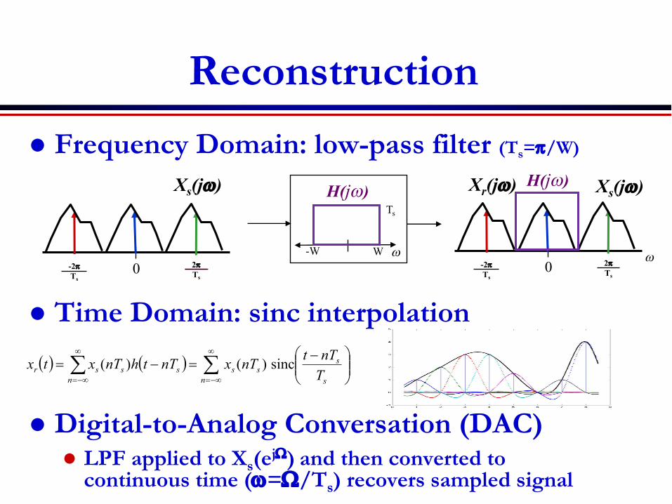
Reconstructionl Frequency Domain: low-pass filter (Ts=p/W)
l Time Domain: sinc interpolation
l Digital-to-Analog Conversation (DAC)l LPF applied to Xs(ejW) and then converted to
continuous time (w=W/Ts) recovers sampled signal
Xs(jw)
0 2pTs
-2pTs
W-W w
Ts
w
H(jw)
0-2pTs
Xs(jw)
2pTs
Xr(jw)
( ) ( ) åå¥
-¥=
¥
-¥=÷÷ø
öççè
æ -=-=n s
sss
nsssr T
nTtnTxnTthnTxtx sinc)()(
H(jw)

Nyquist Sampling Theoreml A bandlimited signal [-W,W] radians is completely described
by samples every Ts£p/W secs.
l The minimum sampling rate for perfect reconstruction, called the Nyquist rate, is W/p samples/second
l If a bandlimited signal is sampled below its Nyquist rate, distortion (aliasing occurs)
Xs(jw)X(jw)
W-W WW
X(jw)
2W=2p/Ts-2W 00

Quantization
l Divide amplitude range [-A,A] into 2N levels, {-A+kD}, k=0,…2N-1l Map x(t) amplitude at each Ts to closest level, yields xQ(nTs)=xQ[n]l Convert k to its binary representation (N bits); converts xQ[n] to bits
-A
A
-A+D-A+2D
-A+kD
……
Ts 2Ts …0
xQ(nTs)x(t)

Continuous-TimeUnquantized
x(t) nTt =Anti-AliasingLowpass Filter
Bandlimits x(t) toprevent aliasing
Sampler
Quantizer
Discrete-TimeUnquantized
xd[n] = x(t)| t = nT
Discrete-TimeQuantized Representation
of xd[n] …
Digital Storage,Transmission,
Signal Processing, …
Discrete-TimeQuantized y[n] Reconstruction
SystemContinuous-Time
y(t)
Analog to Bits and Back
Continuous-TimeUnquantized
x(t) nTt =Anti-AliasingLowpass Filter
Bandlimits x(t) toprevent aliasing
Sampler
Quantizer
Discrete-TimeUnquantized
xd[n] = x(t)| t = nT
Discrete-TimeQuantized Representation
of xd[n] …
Digital Storage,Transmission,
Signal Processing, …
Discrete-TimeQuantized y[n] Reconstruction
SystemContinuous-Time
y(t)
Analog to Bits
Bits to Analog
0100100110010010000100001000100111…
0100100110010010000100001000100111…
ADC
DAC

Sampling with Zero-Order Hold
l Ideal sampling not possible in practicel In practice, ADC uses zero-order
hold to produce xd[n] from x0(t)l Reconstruction of x(t) from x0(t) removes h0(t) distortion
l Multiplication in frequency domain by P 𝝎𝝎𝒔
/H0(jw)
l Also use zero-order hold for reconstruction in practice
R1
R2
xd(t) h0(t)1
Ts
x0(t)Hr(jw)
xr(t)=x(t)DiscreteTo
Continuous
xd[n]=x(nTs)
xs(t)ånd(t-nTs)
0 Ts 2Ts 3Ts 4Ts-3Ts -2Ts -Ts
x(t)´
xs(t) h0(t)1
Ts
x0(t) x0(t)xd[n] (Ts=1)

X(jw)
Xs(jw) |H0(jw)|
|X0(jw)|
|Hr(jw)|
x(t)´
xs(t) h0(t)1
T
x0(t)
ånd(t-nTs)
Hr(jw)xr(t)=x(t)
Ho(jw)Hr(jw)=T&P 𝝎𝝎𝒔
T
Zero-order hold model

l Inserts L-1 zeros between each xd[n] value to get upsampledsignal xe[n]
l Compresses Xd(ejW) by L in W domain and repeats it every 2p/L; So Xe(ejW) is periodic every 2p/L
l Leads to less stringent reconstruction filter design than ideal LPF: zero-order hold often used
Discrete-Time Upsampling
0 1 2 3 4 0 L 2L 3L 4L
xd[n] xe[n]
0 p-pW
Xd(ejW)
WW-WW
WW=WTs
2p-2p W
Xe(ejW)
WW-WW
L L
… …
2pL
-2pL
xe[n]UpsampleBy L (L)
xd[n]=x(nTs)
0w
X(jw)
W-W

Reconstruction of Upsampled Signal
l Pass through an ideal LPF Hi(ejW) to get xi[n] l xi[n]=ẋe[n]=x(nTs/L) if x(t) originally sampled at Nyquist rate (Ts<p/W)l Relaxes DAC filter requirements (approximate LPF/zero-order hold
reconstructs x(t) from xi[n]); better filter to reconstruct from xd[n] needed)
0p-p W
xd[n]=x(nTs)ÛXd(ejW)
WW-WW
Hi(ejW)
2p-2p W
Xe(ejW)
WW-WW
L L
0 L 2L 3L 4L
xe[n]
0 1 2 3 4
xd[n]
xi[n]xe[n]UpsampleBy L
xd[n]=x(nTs)
2pL
-2pL
0 L 2L 3L 4L
xi[n]
Xi(ejW) Û xi[n]Xi(ejW)
x(t)DAC
Reconstruct x(t) from xi[n] by passing it through a DAC
… …
More stringent LPF than for Xd(ejW) Less stringent analog LPFthan to reconstruct from xd[n]
=ẋe[n]
xi[n]=ẋe[n]=x(nTs/L) if Ts<p/W
DiscreteTo Cts Ha(jw)
Ha(ejW)
Ha(ejW)
xi[n] x(t)xr(t)≠x(t)
xd[n]

Digital Downsampling:Fourier Transform and Reconstruction
l Digital Downsamplingl Removes samples of x(nTs) for n≠MTsl Used under storage/comm. constraints
l Repeats Xd(ejW) every 2p/M and scales W axis by Ml This results in a periodic signal Xc(ejW) every 2pl Introduces aliasing if Xd(ejW) bandwidth exceeds p/Ml Can prefilter Xd(ejW) by LPF with bandwith p/M prior to
downsampling to avoid downsample aliasing
xc[n]DownsampleBy M
xd[n]=x(nTs)
0 1 2 3 40 123 …
0 p/M-p/M W’
Xd(ejW’)
0 p-p
Xc(ejW)
-2p 2p
……0 p/M-p/M W’
Xd(ejW’)
0 p-p
Xc(ejW)
-2p 2p
……
W=MW’W=MW’
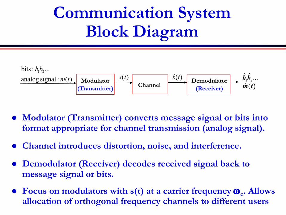
Communication System Block Diagram
l Modulator (Transmitter) converts message signal or bits into format appropriate for channel transmission (analog signal).
l Channel introduces distortion, noise, and interference.
l Demodulator (Receiver) decodes received signal back to message signal or bits.
l Focus on modulators with s(t) at a carrier frequency wc. Allows allocation of orthogonal frequency channels to different users
ChannelDemodulator
(Receiver)Modulator
(Transmitter)
)(ts )(ˆ ts)(ˆ...ˆˆ21
tmbb)(:signal analog
...:bits 21
tmbb

Amplitude ModulationDSBSC and SSB
l Double sideband suppressed carrier (DSBSC) l Modulated signal is s(t)=m(t)cos(wct)l Signal bandwidth (bandwidth occupied in positive frequencies) is 2W
l Redundant information: can either transmit upper sidebands (USB) only or lower sidebands (LSB) only and recover m(t)l Single sideband modulation (SSB); uses 50% less bandwidth (less $$$)
l Demodulator for DSBSC/SSB: downconvert+LPF
))](())(([5.)cos()()( ccc jMjMttmts wwwww ++-Û=)( wjS)( wjM
LSB
USB USB
W-W w wwc-wc
W 2W
wc-wc X
cos(wct)s(t)
2wc0-2wc

AM Radio
l Broadcast AM has s(t)=[1+kam(t)]cos(wct) with [1+kam(t)]>0l Constant carrier cos(wct) carriers no information; wasteful of powerl Can recover m(t) with envelope detector (diode, resistors, capacitor)l Modulated signal has twice bandwidth W of m(t), same as DSBSC
m(t) X
cos(wct)
+
A s(t)=[A+kam(t)]coswct
1/(2pwc)<<RC<<1/(2pW)
ka
1
)( wjM
W-W
ka
wc-wc
)( wjM
W-W

Quadrature Modulation
DSBSCDemod
DSBSCDemod
m1(t)cos(wct)+m2(t)sin(wct)
LPF
LPF
-90o
cos(wct)
sin(wct)
Sends two info. signals on the cosine and sine carriers
m1(t)
m2(t)

l Baseband digital modulation converts bits into analog signals y(t) (bits encoded in amplitude)
l Pulse shaping (optional topic)l Instead of the rect function, other pulse shapes usedl Improves bandwidth properties and timing recoveryl Explored in extra credit Matlab problem
Baseband Digital Modulation
1 0 1 1 0 1 0 1 1 0On-Off Polar
t tTb
)()()(*)()()( bk
kbk
k kTtatxfortrecttxkTtrectatm -==-= åå¥
-¥=
¥
-¥=
d
m(t)m(t)A A
-A

l Changes amplitude (ASK), phase (PSK), or frequency (FSK, no covered) of carrier relative to bits
l We use baseband digital modulation as information signal m(t) to encode bits, i.e. m(t) is on-off or polar
l Passband digital modulation for ASK/PSK is a special case of DSBSCl For m(t) on/off (ASK) or polar (PSK), modulated signal is
Passband Digital Modulation
)cos()()cos()()( tkTtrectattmts cbk
kc ww úû
ùêë
é -== å¥
-¥=

ASK and PSK
l Amplitude Shift Keying (ASK)
l Phase Shift Keying (PSK)
îíì
==
==)"0("0)(0)"1(")()cos(
)cos()()(b
bcc nTm
AnTmtAttmts
ww
1 0 1 1
AM Modulation
AM Modulation
m(t)
m(t)
îíì
-=+=
==)"0(")()cos()"1(")()cos(
)cos()()(AnTmtAAnTmtA
ttmtsbc
bcc pw
ww
1 0 1 1
Assumes carrier phase f=0, otherwise need phase recovery of f in receiver
A
-A
A
-A

ASK/PSK Demodulationl Similar to AM demodulation, but only need to choose
between one of two values (need coherent detection)
l Decision device determines which of R0 or R1 that R(nTb) is closest tol For ASK, R0=0, R1=A, For PSK, R0=-A, R1=Al Noise immunity DN is half the distance between R0 and R1
l Bit errors occur when noise exceeds this immunity
s(t) ´
cos(wct+f)
ò ×bT
b
dtT 0
)(2
nTb
Decision Device
“1” or “0” r(nTb)
R0
R1
a0
r(nTb)
r(nTb)+N
Integrator (LPF)
DN

Quadrature Digital Modulation: MQAM
l Sends different bit streams on the sine and cosine carriersl Baseband modulated signals can have L>2 levels
l More levels for the same TX power leads to smaller noise immunity and hence higher error probability:
l Sends 2log2(L)=M bits per symbol time Ts, Data rate is M/Ts bpsl Called MQAM modulation: 10 Gbps WiFi: 1024-QAM (10 bits/10-9 secs)
● L=32 levels
10 11 00 01
t
mi(t)m1(t)cos(wct)+m2(t)sin(wct)+
n(t)
X
-90o
cos(wct)
sin(wct)
X
ò ×bT
b
dtT 0
)(2
ò ×bT
b
dtT 0
)(2
Decision Device
“1” or “0”
R0
R1
a0
rI(nTb)+NI
Decision Device
“1” or “0”
R0
R1
a0
rQ(nTb)+NQ
A
-A
A/3
-A/3
Ts
Data rate: log2L bits/TsTs is called the symbol time

Introduction to FIR Filter Design
l Signal processing today done digitallyl Cheaper, more reliable, more energy-efficient, smaller
l Discrete time filters in practice must have a finite impulse response: h[n]=0, |n|>M/2l Otherwise processing takes infinite time
l FIR filter design typically entails approximating an ideal (IIR) filter with an FIR filterl Ideal filters include low-pass, bandpass, high-passl Might also use to approximate continuous-time filter
l We focus on two approximation methodsl Impulse response and filter response matchingl Both lead to the same filter design

Impulse Response Matchingl Given a desired (noncausal, IIR) filter response hd[n]
l Objective: Find FIR approximation ha[n]: ha[n]=0 for |n|>M/2 to minimize error of time impulse response
l By inspection, optimal (noncausal) approximation is
[ ] ( )W« jdd eHnh
[ ] [ ] [ ] [ ] [ ] 2/||,0][since,
2
2
2
22 Mnnhnhnhnhnhnh aMn
dMn
adn
ad >=+-=-= ååå>£
¥
-¥=
eDoesn’t depend on ha[n]
[ ] [ ]îíì
>£
=2/02/
MnMnnh
nh da
Exhibits Gibbs phenomenonfrom sharp time-windowing
W
( )Wja eH
p- p0

Frequency Response Matchingl Given a desired frequency response Hd(ejW)
l Objective: Find FIR approximation ha[n]: ha[n]=0 for |n|>M/2 that minimizes error of freq. response
l Set and
l By Parseval’s identity:l Time-domain error and frequency-domain error equall Optimal filter same as in impulse response matching
( ) ( )ò-
WW W-=p
pp
e deHeH ja
jd
2
21
[ ] ( )òå-
W¥
-¥=
W=p
ppdeXnx j
n
22
21
[ ] [ ] [ ]nhnhnx ad -= ( ) ( ) ( )WWW -= ja
jd
j eHeHeXand
[ ] [ ]îíì
>£
=2/02/
MnMnnh
nh da 2/||)(
21][ MndeHnh j
da £W= W
-òp
pp

Causal Design and Group Delayl Can make ha[n] causal by adding delay of M/2l Leads to causal FIR filter design
l If ÐHa(ejW) constant, ÐH(ejW) linear in W with slope -.5Ml Most filter implementations do not have linear
phase, corresponding to a constant delay for all W. l Group delay defined as
l Constant for linear phase filtersl Piecewise constant for piecewise linear phase filtersl Nonconstant group delay introduces phase distortion
relative to an ideal filter
[ ] úûù
êëé -=
2Mnhnh a ( ) [ ] W-
=
W å= jnM
n
j enheH0
( ) ( )WW-W = ja
Mjj eHeeH 2
)( WÐW¶¶
- jeH

Art and Science of Windowingl Window design is created as an alternative to the
sharp time-windowing in ha[n]l Used to mitigate Gibbs phenomenonl Window function (w[n]=0, |n|>M/2) given by
l Windowed noncausal FIR design:
l Frequency response smooths Gibbs in Ha(ejW)
l Design often trades “wiggles” in main vs. sidelobesl Hamming smooths out wiggles from rectangular windowl Introduces more distortion at transition frequencies than rectangle
[ ] ( )W« jeWnw
[ ] [ ] [ ] [ ] [ ]nhnwnhnwnh daw ×=×=
( ) ( ) ( )( ) qp
qp
p
q deHeWeH jd
jjw
-W
-
W ò=21

Typical Window Designs
-5 0 50
0.5
1
n
w[n]
boxcar(M+1), M = 8
-5 0 50
0.5
1
n
w[n]
triang(M+1), M = 8
-5 0 50
0.5
1
n
w[n]
bartlett(M+1), M = 8
-5 0 50
0.5
1
n
w[n]
boxcar(M+1), M = 8
-5 0 50
0.5
1
n
w[n]
triang(M+1), M = 8
-5 0 50
0.5
1
n
w[n]
bartlett(M+1), M = 8
-5 0 50
0.5
1
n
w[n]
hann(M+1), M = 8
-5 0 50
0.5
1
n
w[n]
hanning(M+1), M = 8
-5 0 50
0.5
1
n
w[n]
hamming(M+1), M = 8
-5 0 50
0.5
1
n
w[n]
hann(M+1), M = 8
-5 0 50
0.5
1
n
w[n]
hanning(M+1), M = 8
-5 0 50
0.5
1
n
w[n]
hamming(M+1), M = 8
0 0.5 1 1.5 2 2.5 3-70
-60
-50
-40
-30
-20
-10
0
W
20 lo
g 10|W
(ej W
)|
M = 16
BoxcarTriangular
0 0.5 1 1.5 2 2.5 3-70
-60
-50
-40
-30
-20
-10
0
W
20 lo
g 10|W
(ej W
)|
M = 16
HammingHanning
0 0.5 1 1.5 2 2.5 3
-0.2
0
0.2
0.4
0.6
0.8
1
W
W(ej W
)
M = 16
BoxcarTriangular
0 0.5 1 1.5 2 2.5 3
-0.2
0
0.2
0.4
0.6
0.8
1
W
W(ej W
)
M = 16
HammingHanning

l We are given a desired response hd[n] which is generally noncausal and IIR l Examples are ideal low-pass, bandpass, highpass filtersl May be derived from a continuous-time filter
l Choose a filter duration M+1 for M evenl Larger M entails more complexity/delay, less approximation error e
l Design a length M+1 window function w[n], real and even, to mitigate Gibbs while keeping good approximation to hd[n]
l Calculate the noncausal FIR approximation ha[n]
l Calculate the noncausal windowed FIR approximation hw[n]
l Add delay of M/2 to hw[n] to get the causal FIR filter h[n]
Summary of FIR Design
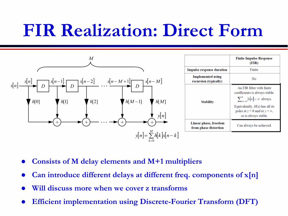
FIR Realization: Direct FormM
[ ]nx
]0[h ]1[h ]2[h ]1[ -Mh ][Mh
++ + +…
…D D D
[ ]1-nx [ ]2-nx [ ]Mnx -[ ]1+-Mnx[ ]nx
[ ] [ ] [ ]å=
-=M
kknxkhny
0
l Consists of M delay elements and M+1 multipliers
l Can introduce different delays at different freq. components of x[n]
l Will discuss more when we cover z transforms
l Efficient implementation using Discrete-Fourier Transform (DFT)
++ + +
…
… [ ] [ ] [ ]å=
-=M
kknxkhny
0++ + +
…
… [ ] [ ] [ ]å=
-=M
kknxkhny
0

Post Midterm Material

Discrete Fourier Series and Transforms
l Discrete Fourier Series (DFS) Pair for Periodic Signals
l Discrete Fourier Transform (DFT) Pair
l and are one period of and , respectively
l DFT is DTFT sampled at N equally spaced frequencies between 0 and 2p:
[ ] [ ] knN
N
k
WkXN
nx --
=å=1
0
~1~ [ ] [ ] knN
N
n
WnxkX å-
=
=1
0
~~
[ ] [ ] knN
N
k
WkXN
nx --
=å=1
0
1 [ ] [ ] knN
N
n
WnxkX å-
=
=1
0
[ ]kX [ ]kX~[ ]nx~[ ]nx
[ ] ( ) 10,2 -££==W
W NkeXkXN
k
jp
𝑥([𝑛] 𝑋-[𝑘] ={𝑁𝑎2}= 𝑥([𝑛]DFS/IDFS IDTFS/DTFS
𝑋 𝑘 = 𝑋 𝑒67 ×S𝑘𝛿 𝑛 − 2p𝑘/𝑁𝑥([n]=𝑥 𝑛 ∗ ∑ 𝛿 𝑛 − 𝑘𝑁�2

DFT/IDFT as Matrix Operation
l DFT
l Inverse DFT
l Computational Complexityl Computation of an N-point DFT or inverse
DFT requires N 2 complex multiplications.
[ ] [ ] knN
N
k
WkXN
nx --
=å=1
0
1
[ ] [ ] knN
N
n
WnxkX å-
=
=1
0

Properties of the DFS/DFT

Key DFT Properties
l Circular Time Shift ® DFT mutiplication with exponential
l Circular Frequency Shift ® multiplication in time by exponential
l Circular convolution in time is multiplication in frequency
l Multiplication in time is circular convolution in frequency
( )( )[ ] [ ] [ ]kXekXWmnxkm
Njkm
NN
p2-
=«-
[ ] [ ] ( )( )[ ]Nln
Njln
N lkXnxenxW -«=-p2
[ ] ( )( )[ ] [ ] [ ]kXkXmnxmxDFTN
mN 21
1
021 «-å
-
=
[ ] [ ] [ ] [ ]kXkXnxnx N 2121 !«× ?@

Computing Circular Convolution;Circular vs. Linear Convolution
l Computing circular convolution:l Linearly convolve and
l Place sequences on circle in opposite directions, sum up all pairs, rotate outer sequence clockwise each time increment
l Matlab Command:
l Circular versus Linear Convolution
[ ] [ ] [ ] [ ]ïî
ïíì
-££-= å-
=
otherwise0
10~~1
021
21Nnmnxmxnxnx
N
mN![ ]nx1~ [ ]nx2~
[ ] [ ] [ ] [ ] [ ] [ ] [ ] [ ] [ ] [ ]13223100 212121210241 xxxxxxxxnxnx n +++==! [ ] [ ] [ ] [ ] [ ] [ ] [ ] [ ] [ ] [ ]23320110 212121211241 xxxxxxxxnxnx n +++=
=!
[ ] ][21 nxnx =
n0 3
1
1 2
[ ] [ ]nxnx 21 4
n0 3
4
1 2
x1[n] * x2[n]
n0 3
1
1 2 64 5
1
2 2
3 3
4
y = ifft(fft(x1,N).*fft(x2,N))

Linear Convolution using Circular Convolution
l Want to linearly convolve two sequencesl e.g. to obtain the output of a filter to an input sequence
● x[n] has length L, h[n] has length P, y[n] has length L+P-1
l Obtain linear convolution as follows:l Zero pad x[n] by appending P-1 zeros to get xzp[n]; 0£n£L+P-2l Zero pad h[n] by appending L-1 zeros to get hzp[n]; 0£n£L+P-2l Both sequences are of length M=L+P-1, same as y[n]l Take circular convolution of zero padded sequences l This yields the linear convolution:
● Zeros padding removes circular effect
[ ] [ ] [ ] [ ] [ ] [ ] [ ]mhmnxmnhmxnhnxnyP
m
L
måå-
=
-
=
-=-==1
0
1
0
*
, the same as the linear convolution .

Example: Linear from Circularl Linear Convolution
l Linear from Circular with Zero Padding
][2 nx
n0 3
1
1 2
x1[n] * x2[n]
n0 3
1
1 2 64 5
2
3
4
n0 3
1
1 2 4 5
[ ]nx1
87
1
2
3
4 4
][,2 nx zp
n0 3
1
1 2
0 3
1
1 2 4 5
[ ]nx zp,1
L=4
P=6
M=L+P-1=9
64 5 7 8
n6 7 8
[ ] [ ] 4|21 6 =nnxnx
n0 3
4
1 2 54
1 1
1
1
00
0
0
0
1 0
0
0
11
1
1
1
n=0
1 1
1
1
00
0
0
0
1 1
0
0
01
1
1
1
n=1
[ ] [ ]nxnx zpzp ,2,1 9

Block Convolution using Overlap Methods
l Want block-by-block linear convolution for long sequencesl Uses fixed hardware. Has fixed delay/complexity
l Goal: compute linear convolution of x[n] and y[n]l x[n] very long, h[n] has length Pl Want to break x[n] into shorter blocks and compute portions of
y[n] block-by-block.
l Overlap-Add Methodl Breaks x[n] into non-overlapping segments of length L:
l Convolve each segment with h[n] and sum: l These convolutions computed using DFT (zero padding):
[ ] [ ] [ ] [ ] [ ] [ ] [ ]mhmnxmnhmxnhnxnyP
mmåå-
=
¥
=
-=-==1
00
*
[ ] [ ]å¥
=
=0r
r nxnx
[ ] [ ] [ ] [ ] [ ]å¥
=
==0
**r
r nhnxnhnxny
[ ] [ ] ( )îíì -+££
=otherwise0
11 LrnrLnxnxr


Blocklength Choicel In overlap methods, several factors affect the
choice of the block length Ll a shorter block length minimizes latency.l a shorter block length minimizes memory required for
performing the DFTs, multiplication, and inverse DFT.
l Given P (length of h[n]), there is an optimal block length L that minimizes complexity. l L too short, complexity increased by overhead of
adjacent block overlap l L too long, complexity increased because DFT
complexity increases with the block length l In practice, set block length so that DFT blocklength is
an integer power of 2 (required for FFTs)

FFT and IFFT Algorithmsl FFT computes the DFT of a sequence, IFFT
computes the inverse DFT:l DFT as matrix operation: N2 complex multipliesl Complexity of FFT and IFFT same:
l FFT/IFFT breaks down a DFT with N2 complex multiplies into many smaller DFTs with N multipliesl Not responsible for details of how this is done (pp. 107-113 of reader, end of chapter 4)
l Reduces complexity of computing N-point DFT or IDFT from N2 complex multiplies to .5Nlog2N
N N2 NN22 log
NN
N22
2
log
16 256 32 8.0
128 16,384 448 36.6
1,024 1,048,576 5,120 204.8
8,192 67,108,864 53,248 1260.3
- In 1994 Strang described the FFT as "the most important numerical algorithm of our lifetime”- Included in Top 10 Algorithms of 20th Century by IEEE Journal of Computing in Science and Engineering
[ ] [ ] knN
N
n
WnxkX å-
=
=1
0
[ ] [ ] knN
N
k
WkXN
nx --
=å=1
0
1
[ ]{ } [ ]{ }( )**1 1 kXDFTN
kXDFT =-
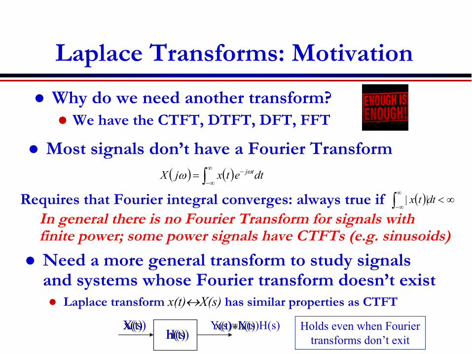
Laplace Transforms: Motivationl Why do we need another transform?
l We have the CTFT, DTFT, DFT, FFT
l Most signals don’t have a Fourier Transform( ) ( ) dtetxjX tjww -¥
¥-ò=Requires that Fourier integral converges: always true if ( ) ¥<ò
¥
¥-dttx ||
l Need a more general transform to study signals and systems whose Fourier transform doesn’t existl Laplace transform x(t)«X(s) has similar properties as CTFT
In general there is no Fourier Transform for signals with finite power; some power signals have CTFTs (e.g. sinusoids)
x(t)h(t)
x(t)*h(t)X(s)H(s)
Y(s)=X(s)H(s) Holds even when Fouriertransforms don’t exit

Laplace Transform Definition and Region of Convergence (ROC)
l Bilateral Laplace transform l Always exists within a Region of Convergencel Used to study systems/signals w/out Fourier Transforms
l Generalizes Fourier Transform:
l Region of Convergence (ROC):l All values of s=s+jw such that L[x(t)] existsl Depends only on s
l Example
( )[ ] ( ) ( ) ( ) ¥<+=== òò¥
¥-
--¥
¥-
dtetxjsdtetxsXtxL tst sws ifexists;,
( )[ ] ( )[ ]tetxFtxL s-= ( ) ( ) ( )[ ]txFjXsX js ===
ww
Defn:
wj
s
X(s)definedin ROC
X(jw)
Smallest s:X(s) exists
strips alongjw axis
Plotted on s-plane( )tue at- ( ) as ->Re( ) ,1
assX
+=L

OWN pg. 691, Reader pp. 20-27
(Similar to CTFT propertiesReplace jw with s, check ROC)
Used for LTISystems Analysis
Used to solve ODEs
Applies to causal signals;Useful to check initial and final
values of x(t) without inverting X(s)0 Error in OWN, has ∞ instead of 0

OWN pg. 692
(Similar to CTFT pairs
Replace jw with s, check ROC)

Systems Analysis with Laplace
l LTI Analysis using convolution property
l Equivalence of Systems
( )tx ( )ty( ) ( )thtg +
( ) ( )sHsG +
( )tx ( )ty( ) ( )thtg *
( ) ( )sHsG ×( )tx ( )ty
( )tg( )sG
( )th( )sH
( )tx ( )ty
( )tg( )sG
( )th( )sH
S+
+
( )tx ( )ty( )th( )sH
)(*)()( thtxty =
)()()( sXsHsY =H(s) is system
transfer functionROC is at least ROCxÇROCh

Inverting Laplace Transforms and its Rational Form
l Inverse Laplace transformsl Can apply inverse Fourier:
● Complex integration part of complex analysis (Math 116)l Can obtain inverse for rational Laplace transform using
simple math (partial fraction expansion)
l Rational Laplace Transforms
l Zeros and Poles:l bs are zeros (where X(s)=0), gs are poles (where X(s)=¥)l ROC cannot include any polesl If X(s) real, all zeros of X(s) are real or occur in complex-conjugate
pairs. Same for the poles.l bM/aN, zeros, poles, and ROC fully specify X(s)
( ) ( )( )
( )( ) ( )( )( )( ) ( )( )NN
MM
N
MN
NN
N
MM
MM
ssssssss
ab
sasasaasbsbsbb
sAsBsX
ggggbbbb
--------
=++++++++
==-
--
-
--
121
1211
110
1110
!!
!! …
…
( ) ( )[ ] ( ) wwsp
ws ws dejXjXFetx tjt ò¥
¥-
-- +=+=211
……

More on Laplacel ROC for Right, Left, and Two-Sided Signals
l Right-sided: x(t)=0 for t<a for some a● ROC is to the right of the rightmost pole, e.g. RH exponential
l Left-sided: x(t)=0 for t>a for some a● ROC is to the left of the leftmost pole, e.g. LH exponential
l Two-sided: neither right or left sided● ROC is a vertical strip between two poles, e.g. 2-sided exponential
l Magnitude/Phase of Fourier from Laplacel Given Laplace in rational form with jw in ROC
l Can obtain magnitude and phase from individual components using geometry, formulas, or Matlab
( )( )
( )Õ
Õ
=
=
-
-= N
kk
M
kk
N
M
s
s
absH
1
1
g
b
( )( )
( )Õ
Õ
=
=
-
-= N
kk
M
kk
N
M
j
j
abjH
1
1
gw
bww
( )Õ
Õ
=
=
-
-= N
kk
M
kk
N
M
j
j
ab
jH
1
1
gw
bww
( ) ( ) ( )åå==
-Ð--Ð+÷÷ø
öççè
æÐ=Ð
N
kk
M
kk
N
M jjabjH
11
gwbww

Example: First-order LPF“s-domain circuit analysis of KVL equations”
( )÷ø
öçè
æ÷øö
çèæ--
=+
==
ttt 1
111
)()(
sssHsYsH
RC=t
( ) ( )gwtwtw
-=
+=
jjjH 1
11
21
( )wjH
w
0t1
-t1
1
( )wjHÐ
t1
0
4p
4p
-
2p
2p
-
t1
-w
( ) t=Ð-
=0ωdωjωHd
}/1{ ts ->=ROC
ROC
( ) ( )tttt)()()(11 sXsYssYtxty
dtdy
=+®=+
h(t) causal, so the ROC is right-sided, and H(jw) existsÞ ROC defined implicitly

Bode Plot for 1st Order LPF
t01.0
20 lo
g 10|H
(jw)|
(dB
)
t1.0
t1
t10
t100
w
0
20-
40-
30-
10- tw 1for dB 0 <
tw 1for dB/decade 20 >-
BodeExact
ÐH
(jw) (
rad)
BodeExact
t01.0
t1.0
t1
t10
t100
w
2p
-
4p
-
0
tw 1.0for rad 0 <
twp 10for rad
2>-
twp 1for rad
4=-
l Bode Plots: show magnitude/phase on dB scalel Plots 10log10|H(jw)|2=20log10|H(jw)| vs. w (dB)l Can plot exactly or via straight-line approximationl Poles lead to 20dB per decade decrease in Bode plot, Zeros lead to 20
dB per decade increasel Frequency w in rad/s is plotted on a log scale for w³0 only

Inversion of Rational Laplace Transforms
l Extract the Strictly Proper Part of X(s)l If M<N, is strictly proper, proceed to next stepl If M³N, perform long division to get , where
l Invert D(s) to get time signal:
l Follows from and
l The second term is strictly proper
l Perform a partial fraction expansion:
l Invert partial fraction expansion term-by-terml For right-sided signals:
( ) ( )( ) N
NN
N
MM
MM
sasasaasbsbsbb
sAsBsX
++++++++
== --
--
1110
1110
!!
( ) ( )sXsX ~=
,
( ) ( ) ( )sXsDsX ~+=
( ) 011
1 dsdsdsdsD NMNM
NMNM ++++= --
---
- !
( ) ( )( ) ( )( ) ( )( ) ( )( ),00
11
11 tdtdtdtdtd NM
NMNM
NM dddd ++++= ----
-- !
( ) ( ) ( )n
nn
dttdt dd = ( ) ( )sZs
dttzd nn
n
«
( ) ( ) ( )sAsBsX /~~ =
( ) ( )( )
( )
( )Õ=
-== N
kk
N
s
sBa
sAsBsX
1
~1~~
g( )
( )
( ) ( )Õ+=
--= N
pkk
p
N
ss
sBasX
11
~1~
gg( )
( ) åå+== -
+-
=N
pk k
kp
mm
m
sA
sAsX
11 1
1~gg Obtain coefficients via residue method
( ) ( ) ( ) ( )åå+==
-
+-
=N
pk
tk
p
m
tm
m tueAtuemtAtx k
11
1
11
!1~ gg
Need to check ROC
…
…
…

Causality and Stability in LTI Systems
l Causal LTI systems: impulse response h(t)«H(s)l LTI system is causal if h(t)=0, t<0, so is h(t) right-sidedl For H(s) rational, a causal system has its ROC to the right of the
right-most polel Step response is h(t)*u(t) «H(s)/s
l Stable LTI Systeml LTI system is bounded-input bounded-output (BIBO) stable if all
bounded inputs result in bounded outputs. ● We equate BIBO stability with stability; there are other definitions of stability
l A system is stable iff its impulse response is absolutely integrable;implies H(jw) exists, equivalently jwÎROC
l A system H(s) is stable iff H(s) strictly proper and jwÎROC
l A causal system with H(s) rational is stable if & only if all poles of H(s) lie in the left-half of the s-planel Equivalently, all poles have Re(s)<0l ROC defined implicitly for causal stable LTI systems

LTI Systems Described by Differential Equations (DEs)
l Finite-order constant-coefficient linear DE system
l Poles are roots of A(s), zeros are roots of B(s)l If system is causal (pp. 184 of reader):
l for x(t)=d(t), initial conditions are zero: y(0-)=y(1)(0-)=…=y(N-1)(0-)=0l ROC of H(s) is right-half plane to the right of the right-most pole
l Can solve DEs with non-zero initial conditions using the unilateral Laplace transform:l Not covered in this class as we focus on causal stable systemsl Extra credit reading: “Laplace” pp. 180-185 (177-182) of Reader
( ) ( )åå==
=M
kk
k
k
N
kk
k
k dttxdb
dttyda
00
( ) ( )sXsbsYsaM
k
kk
N
k
kk ×÷÷
ø
öççè
æ=×÷÷
ø
öççè
æåå== 00
( )å
å
=
=== N
k
kk
M
k
kk
sa
sb
sAsBsH
0
0
)()(
( )[ ] ( ) ( ) dtetxsXtxL stuu
-¥
ò-
==0

Second Order Lowpass System
l We first factor H(s):
l Three regimes for H(jw) :l Underdamped: 0<z<1, gs distinct, complex conjugatesl Critically Dampled: z=1, gs equal and reall Overdamped: 1<z<¥, gs distinct and real
R L
C+
-x(t) y(t)
+
-
LCn1
=w mk
n =w
LCR
2=z km
b2
=z
( ) ( )txtydtdy
dtyd
nnn22
2
2
2 wwzw =++ ( ) ( ) ( )sXsYss nnn222 2 wwzw =++ ( ) ( )
( ) 22
2
2 nn
n
sssXsYsH
wzww
++==
natural frequency wn and damping coefficient z
( ) ( )( ) ,21
2
ggw
--=
sssH n ( )12
21 --= zzwg !n
Poles inleft-half
of s-planeh(t) causal
H(jw) exists
±

Frequency Response: ( )( ) ( ) 22
2
2 nn
n
jjjH
wwzwww
w++
=
l Underdamped: 0<z<1, gs distinct, complex conjugatesl Critically Dampled: z=1, gs equal and reall Overdamped: 1<z<¥, gs distinct and real

Feedback in LTI Systems
l Motivation for Feedbackl Can make an unstable system stablel Can make transfer function closer to desired (ideal) onel Can make system less sensitive to disturbancesl Can have negative effect: make a stable system unstable
l Transfer Function T(s) of Feedback System:
( )tx ( )ty( )( ) ( )sHsGsG
!1
( )tx ( )ty( )tg( )sG
( )th( )sH
S+ ( )te
±
Equivalent System
( )( )
( )( ) ( )sHsGsG
sXsYsT
!1)( ==Y(s)=G(s)E(s); E(s)=X(s)±Y(s)H(s)
±
±

Two Examplesl Stabilizing an unstable system: 1st order system
l a>0, pole in right-half of s-plane
l System is stable if K>a, single pole in left half of s-plane
l Feedback can make a stable system unstable
as -1
K
S+
-x(t)
e(t)
r(t)
y(t)
( ) sTeKKKsT --
=21
1
1
Unstable if K1K2>1

Bilateral Z-TransformDiscrete Time; Analysis very similar to Laplace
l Generalizes Discrete-Time Fourier Transforml Always exists within a Region of Convergencel Used to study systems/signals without DTFTs
l Relation with DTFT:
l Region of Convergence (ROC):l All values of z such that X(z) existsl Depends only on r (vs. s in Laplace)
● Circles instead of planes
l Example:
{ } ( ) ¥<==== åå¥
-¥=
-W¥
-¥=
-
n
njz
n
n rnxreezzznxzXnxZ ][ifexists;||,][][ !
{ }nrnxDTFTzX -= ][)( ( ) ( ) ]}[{1||
nxDTFTeXzX jzr
== W==
Defn:
Smallest r:X(z) exists
Circles in z-plane
Plotted on z-plane|||| az >][nue at- ( ) ,1
azzX
+=Z
True for some rÎR

Rational Z Transformsl Numerator and Denominator are polynomials
l Alternate form:
l bs are zeros (where X(z)=0), gs are poles (where X(z)=¥)l ROC cannot include any polesl If X(z) real, a’s and b’s are real ® all zeros of X(z) are real
or occur in complex-conjugate pairs. Same for the poles.l bm/an, zeros, poles, and ROC fully specify X(z)l Example: 2-sided exponential
( ) ( )( )( )1
1
-
-
---
=bzbzzbbzX[ ] [ ] [ ]1--+= - nubnubnx nn
…
…


ROC for “Sided” Signalsl Right-sided: x[n]=0 for n<a for some a
● ROC is outside circle associated with largest pole● Example: RH exponential: x[n]=anu[n]
l Left-sided: x[n]=0 for n>a for some a● ROC is inside circle associated with smallest pole● Example: LH exponential: x[n]=-anu[-n-1]
l Two-sided: neither right or left sided● Can be written as sum of RH and LH sided signals● ROC is a circular strip between two poles● Example: 2-sided exponential: x[n]=b|n|, b<1

l Extract the Strictly Proper Part of X(s)l If M<N, is strictly proper, proceed to next stepl If M³N, perform long division to get , where
l Invert D(s) to get time signal ( ; )
l Follows from z-transform table
l The second term is strictly proper
l Perform a partial fraction expansion:
l Invert partial fraction expansion term-by-term (check ROC)l For right-sided signals:
Inversion of Rational z Transforms( ) ( )
( ) NN
NN
MM
MM
zazazaazbzbzbb
zAzBzX
++++++++
== --
--
1110
1110
!!
( ) ( )zXzX ~=
,
( ) ( ) ( )zXzDzX ~+=
( ) 011
1 dzdzdzdzD NMNM
NMNM ++++= --
---
- !
( ) ( ) ( )zAzBzX /~~ =
( ) ( )( )
( )
( )Õ=
-== N
kk
N
z
zBa
zAzBzX
1
~1~~
g
( )( )
( ) ( )Õ+=
--= N
pkk
p
N
zz
zBazX
11
~1~
gg( )
( ) åå+== -
+-
=N
pk k
kp
mm
m
zA
zAzX
11 1
1~gg
Obtain coefficients via residue method
( ) åå+==
+-
-+++=
N
pk
nkk
np
mm
n nuAnum
mnnAnuAnx1
12
1111 ][][!1
)1)...(1(][][~ ggg
[ ] ( )[ ] ( )[ ] [ ] [ ]ndndNMndNMndnd NMNM dddd 011 11 +-++---+--= --- !
…
…
…
…

LTI Systems Analysis using z-Transformsl LTI Analysis using convolution property
l Equivalence of Systems same as for Laplacel G[z] & H[z] in Series: T[z]=G[z]H[z]; in Parallel: T[z]=G[z]+H[z]
l Causality and Stability in LTI Systemsl System is causal if h[n]=0, n<0
● ROC outside circle associated with largest pole since h[n] right sidedl Causal system (BIBO) stable if bounded inputs yield bounded outputsl BIBO stable implies that h[n] absolutely summable Þ H(ejW) existsl H(z) is stable Û H(z) strictly proper and poles inside unit circle, i.e.
r=1ÎROC (see Reader)
][nx ][ny][nh
( )zH
][*][][ nhnxny =
][][][ zXzHzY =H[z] called the transfer function of the system
ROC is at least ROCxÇROCh

Example: Second Order System with Feedback
l Z-Transform
l DTFT: l Exists when r<1l Lowpass filter for q=0l Bandpass filter for q=p/2l Highpass filter for q=p
l Impulse Response (LPF: q=0)
( ) ( )( ) rzzrezrezrzr
zH jj >--
=+-
= ----- ||,111
cos211
11221 qqq
( )WjeH
Wp- p
25
0
r = 0.8, q = p/2
r = 0.8, q = 0
20
15
10
5
p-
p
( )WÐ jeH
Wp- p0
r = 0.8, q = p/2
r = 0.8, q = 0
( )W-W-
W
+-= 22cos21
1jj
j
erereH
q
( )( )211
1--
=rz
zH [ ] ( )[ ] [ ]nurnnh n1+=
Poles at re±jq

Feedback in LTI Systems
l Motivation for Feedbackl Can make an unstable system stable; make a system
less sensitive to disturbances; make it closer to ideall Can have negative effect: make a stable system unstable
l Transfer Function T(z) of Feedback System:
l Example: Population Growth: y[n]=2y[n-1]+x[n]-r[n]l Stable for b<.5
Equivalent System
( )( )
( )( ) ( )zHzGzG
zXzYzT
!1)( ==Y(z)=G(z)E(z); E(z)=X(z)±Y(z)H(z)
( )tx ( )ty( )( ) ( )zHzGzG
!1][nx ][ny
][ng
)(zG
][nh
)(zH
S+ ][ne
±
1)1(211)( ---
=z
zTb

LTI Systems Described by Difference Equations
l DT systems implemented with delay/amplifier elements
l A system with output feedback generally has infinite impulse response
l LTI Systems described by differential equations
l Can write in terms of output at time n
[ ] [ ]åå==
-=-M
kk
N
kk knxbknya
00
( ) ( )zXzbzYzaM
k
kk
N
k
kk ×÷÷
ø
öççè
æ=×÷÷
ø
öççè
æåå=
-
=
-
00( ) ( )
( )zAzB
za
zbzH N
k
kk
M
k
kk
==
å
å
=
-
=
-
0
0

Direct Form Implementation of IIR Filters/Systems H(z)
Approximates continuous time filters with lower
complexity than FIR designs

IIR Filter Design
l Discussed FIR filter design of hw[n] for desired IIR noncausal filter Hc(jw) before MTl Convert Hc(jw) to DT IIR filter as Hc(jw)ÞHd(ejW) for W=wT
l Now consider design of IIR H(z) to approximate Hc(s)l Have more tools at our disposal for this design (z-transforms)l Low complexity implementation of IIR filters vs FIR (via feedback)l Two methods: temporal and frequency response matchingl Temporal (not on HW/exam): Design H(z) so that for a given x(t)
(impulse, step), yd[n]=yc(nT); introduces aliasing if T>p/W
x(t)Hc(s)
yc(t)
ADCSample time T
H(z) DACyd(t)yd[n]x[n]

Frequency Response (FR) Matching
Can use more general mappingfor any real C, 0<C∞
l FR Matching: Bilateral Transform (BLT)l Nonlinear invertible mapping between s-plane and z-plane
l Discrete time filter design of H(z) under BLT:l Ensures that if Hc(s) stable, H(z) also stable with no aliasingl There is warping due to nonlinear mapping, esp. at high frequencies
l Mapping between s and z plane:l s=0 yields |z|=1 l jw axis in s-plane Þ unit circle in z-planel left/right half of s-plane Þ inside/outside unit circlel Left-half poles of s-plane map inside circle
● Stability preserved in the mapping to H(z)

s/z plane mapping
l Phase:
l So entire jw axis of s-plane mapped to one revolution of the z-plane along unit circle ● No aliasing of the frequency response, but warps
W@wT for |w|<<p/T
-p<W<p-∞<w< ∞

M
[ ]nx
]0[h ]1[h ]2[h ]1[ -Mh ][Mh
++ + +
…
…
D D D[ ]1-nx [ ]2-nx [ ]Mnx -[ ]1+-Mnx[ ]nx
[ ] [ ] [ ]å=
-=M
kknxkhny
0
FIR versus IIR Implementation
FIR
IIR

Example: 2nd order Butterworth
l BLT:
l IR


Main EE102b Takeaways
l Continuous signals/systems appear in nature
l Data processing and storage typically done digitally due to smaller size, lower power consumption, lower cost, better performancel Hence signal and system inputs/outputs often discrete
l Widespread applications for signals and systems analysis tools
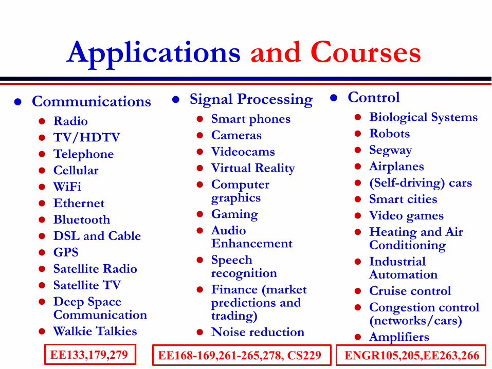
Applications and Coursesl Communications
l Radiol TV/HDTVl Telephonel Cellularl WiFil Ethernetl Bluetoothl DSL and Cablel GPSl Satellite Radiol Satellite TVl Deep Space
Communicationl Walkie Talkies
l Control l Biological Systemsl Robotsl Segwayl Airplanesl (Self-driving) carsl Smart citiesl Video gamesl Heating and Air
Conditioningl Industrial
Automationl Cruise controll Congestion control
(networks/cars)l Amplifiers
l Signal Processingl Smart phonesl Camerasl Videocamsl Virtual Realityl Computer
graphics l Gamingl Audio
Enhancementl Speech
recognitionl Finance (market
predictions and trading)
l Noise reduction
EE133,179,279 EE168-169,261-265,278, CS229 ENGR105,205,EE263,266

Good luck on Finals
Have a Great


