

90 | P a g e
International Journal of Petroleum and Geoscience Engineering
Volume 03, Issue 02, Pages 90-99, 2015 ISSN: 2289-4713
Effects of Increment or Decrement Operational Factors on Asphaltene
Deposition in Shahid Mansoori Oilfield of Iran
Majid Mohammadi a,*, Abass Naderifar a
a Department of Chemical Engineering, Amirkabir University of Technology (Tehran polytechnic), Tehran, Iranb
* Corresponding author.
E-mail address: [email protected]
A b s t r a c t
Keywords:
Asphaltene,
Precipitation,
APP diagrams,
Reservoir.
In this article asphaltene precipitation models are described and in a case study the precipitated
asphaltene is represented by an improved solid model. The main purpose of this study is to
model and anticipate the effects of major parameters on formation of asphaltene precipitation
and deposition at reservoir conditions, in order to provide a better understanding of the factors
that may enhance asphaltene precipitation or deposition. The oil and gas phases are modeled
with Peng-Robinson equation of state. The effect of several factors such as solid molar volume
and injected solvent gas composition as well as thermodynamic condition variations (such as
pressure and temperature) on the predictions made by this model will be investigated too.
Eventually, with regard to the experimental data that has been obtained from one of the oil
wells located at the South Oil Zones of Iran’s oilfields, the accuracy of modeling and
anticipating of asphaltene precipitation will be checked. All of the related calculations have
been done by Winprop software from CMG package.
Accepted: 13 June 2015 © Academic Research Online Publisher. All rights reserved.
1. Introduction
Nowadays the asphaltene deposition’s problems in oil
industries are growing much higher compare to the
past time. These depositions can be seen especially
during the solvent gas injection for enchanted oil
recovery and also after a certain part of well’s life has
been passed (at the same time that pressure drop in the
well starts). Obviously for fully understanding the
asphaltene deposition problems and performing
effective preventive procedures for confronting with
this phenomenon; there should be a comprehensive
study about the effective parameters and related
factors that have the most influence on this topic. The
main goal of this article is considering and analyzing
such reviews. We also should mention that there are
some differences between the Deposition and
Precipitation, deposition is occurring when asphaltene
is separated from crude oil and forming a single solid
phase whereas Precipitation occurs when asphaltene
sticks to a solid surface like pipes or oil stone
surfaces. Therefore the problems which are made by
asphaltene precipitation can be removed by proper
anticipation and exact controlling of asphaltene
deposition. On other words, asphaltene precipitation
can be formed only when asphaltene deposition
occurs. Since that recognizing asphaltenes behavior,
need complete and comprehensive information about
crude oil compositions, first of all we will pay
attention to expression generalities about crude oil
compositions properties.
2. Reviewing the Thermodynamics Models for
Asphaltene Precipitation
The most important models that have been presented
and developed so far are these models:

Majid Mohammadi et al. / International Journal of Petroleum and Geoscience Engineering (IJPGE) 3 (2): 90-99, 2015
91 | P a g e
A. Dissolving Model (1984)
With regards to the common definitions for asphaltene
(like its solubility in aromatics) a thermodynamic
model can be developed for asphaltene deposition.
Hirschberg et al. [1] presented a model by using these
definitions and assumptions. In this model, the related
calculations to liquid and gas phases equilibrium and
flash calculation has been done by SRK equation of
state [2]. In this model it is assumed that asphaltene
deposition (if formation be done) has no effect on gas
liquid equilibrium. By defining the maximum volume
of solved asphaltene in the oil in form of maxa ; this
model can be presented as equation 1:
2
1
11
1
max1ln a
a
a
aRT
v
v
v
v
v (1)
In this equation, the molar volume of asphaltene is a
function of its molar weight and specific weight. As
regards to this fact that almost all of the developed
methods for determination of molecular weight are
relating to molecular collision effects in solution, the
exact value of maxa is not measurable at equation 1
and this is the biggest weak point of this equation.
Solubility parameter, in this equation can be
estimated by determination of solubility amount of
asphaltene in different solvents and specifying the
way that asphaltene react with these solvents per
increasing asphaltene solubility. Therefore, asphaltene
solubility parameter is reported as the asphaltene
dissolution on the best solvent. This parameter also
can be defined as a linear function of temperature as
equation 2:
bTa (2)
Where ‘a’ and ‘b’ are constants [3].
B. Thermodynamic Model of Collision (1987)
With assuming asphaltene as a suspended solid
particle within crude oil which is surrounded by
resins; Mansoori presented a thermodynamic model.
In this model, according to experimental data about
initial point of asphaltene forming, a critical chemical
potential is estimated for resins and then this critical
chemical potential can be used for anticipation of the
initial deposition point in other conditions [4].
C. Thermodynamic Model of Micellars Formation
(1987)
According to formation method of asphaltene
sediment cells which known as micellars and
minimizing Gibbs energy, Firozabadi&Pen presented
thermodynamic model for asphaltene deposition. This
model is highly accurate and can confirm the
experimental data with high precision. Nevertheless
some efforts for improving this model are in progress
that has had no success so far [4].
D. Solid Model (1988)
This model is one of the simplest models for
anticipating asphaltene deposition which asphaltene
assume as a pure solid and single phase within oil and
its gaseous solution. In this model oil and gas phase
behavior is simulating by cubical equation of state.
Pure solid fugacity (asphaltene) can be determined
from equation 3 as below:
RT
PPvff s
ss
**
lnln
(3)
It is worth mentioning that some of the experimental
data which gained by scientists was used for testing
above equation and the result was not very satisfactory
for a part of these data [5]. The other presented
models for asphaltene deposition are generally
complex and have too many configurable parameters
that lead to a more complicated model. An overall
comparison between the presented models will be
discussed in next section of this article.
3. Comparison of Models
Model 4 (solid model) was based on calculation of
fugacities while models 1-3 were formed according to
activity factors. Solid model is using the same
components that were used in equations of state for
modeling of gas and oil phase, while in two previous
models, first gas-oil two phase flash calculations have
been done for dividing oily mixture into oil and gas
phase and then oil phase is divided into different
components for modeling of asphaltene deposition. So
that in model 1 the oil phase is divided into two
components which asphaltenes contain one of these
components and the other component includes non-
asphaltenes. In models 2 and 3 an extra component for
including the micellars and along resins effect on
simulating has been applied.
Majid Mohammadi et al. / International Journal of Petroleum and Geoscience Engineering (IJPGE) 3 (2): 90-99, 2015
92 | P a g e
Although that deposition rate clearly has influence on
oil and gas phase equilibrium, the first three models
neglects this effect, which this ignoring may lead to
occurring some errors in oil-gas phase calculations
(note that heavy components like asphaltene have
major effects on equilibrium conditions of saturated
vapor solution).
Briefly, if the purpose of simulation is applying
thermodynamic model with a multi-components
modeling, using model 4 is recommended. This
exclusive property makes model 4 (solid model) one
of the best possible choice for usage in related
simulating programs like Winprop.
4. CASE STUDY
In this section according to experimental data that is
gained from one of the oil reservoirs in south of Iran,
suggested thermodynamic models in Winprop
software (from CMG software package) will be
investigated and the results will be compared with
experimental data. Eventually to anticipate the amount
of thermodynamic equilibrium conditions (such as
temperature, pressure, oil molar fraction and …)
effects on increasing or decreasing of asphaltene
deposition, these results will be used too.
Tables 1, 2 and 3 are showing overall properties of
crude oil and thermodynamic conditions of reservoir
during oil extraction.
Table 1: Reservoir oil properties.
Value Unit
Reservoir temperature 378.7 K
Saturated pressure 9515 Kpa
Asphaltene volume
percentage
7.71 %Wt
Reservoir oil molecular
weight
166 --
GOR 278.35 SCF/STB
Table 2: Heavy components properties.
Value
Molecular weight of heavy components
C12+
330
Molecular weight of C12+ 0.9636
Table 3: Crude oil composition in one of the southern
Iranian oilfield.
Components Oil Reservoir
(%mol)
C1 19
C2 7.1
C3 5.21
iC4 1.11
nC4 2.9
iC5 1.1
nC5 1.1
C6 5.4
C7 4.1
C8 3.4
C9 3.07
C10 2.95
C11 2.59
C12+ 39.62
N2 0.3
CO2 0.9
A. Specifying Asphaltene Component
The very first step in simulation is specifying the
related asphaltene components. Using separation or
accumulation abilities in Winprop software can help
us to reach this goal. C12+ components can be broken
up to C21+ or C31+, in both case those components
will mark as Ultra heavy or asphaltene part of oil.
Therefore, if we want to divide the components up to
C21+ by using the approved methods, it is necessary
to have an estimate about critical and physical
conditions of divided hydrocarbon groups such as IC4-

Majid Mohammadi et al. / International Journal of Petroleum and Geoscience Engineering (IJPGE) 3 (2): 90-99, 2015
93 | P a g e
NC4 ،IC5-C6، C7-C15، C16-C20 and C21+. The critical
conditions estimate for heavy components with having
some data about special mass and molecular weights
of C21+ component, is calculating by Lee-Kesler
equations [6], [7]. Physical conditions of mixture are
estimated by Teo equations. Applying regression
analysis on hydrocarbon heavy group’s data for
achieving more accurate and valid results seems
essential of course. This analysis applies by Winprop
software itself. It should be mentioned that the oil and
gas phase have been modeled by Peng-Robinson
equation of state [8]. Table 4 shows the crude oil
sample data after regression and dividing the heavy
component up to C21+. Similarly these divisions are
applicable up to C31+ group. Table 5 shows these
results after regression analysis. To determine which
components of asphaltene will sediment for certain,
we need to divide heavy component (such as C21+ or
C31+) into two different parts, one part that is able to
sediment and the other part, which is not able to
sediment.
Table 4: Crude oil component’s properties (after lumping to C21+).
Pc(atm) Tc(K) ω Mw Z Vc(l/mol) SG Mol%
CO2 72.8 304.2 0.225 44.01 0.2736 0.094 0.818 0.93
N2 33.5 126.2 0.04 28.013 0.2905 0.0895 0.809 0.3
C1 45.4 190.6 0.008 16.043 0.2876 0.099 0.3 18.91
C2 48.2 305.4 0.098 30.07 0.2789 0.148 0.356 7.2
C3 41.9 369.8 0.152 44.097 0.2763 0.203 0.507 5.21
IC4-NC4 36.679 422.805 0.208199 58.124 0.27182 0.2582 0.57827 4.04
IC5-C6 31.792 499.214 0.260697 81.1134 0.26541 0.3446 0.66932 7.66
C7-C15 28.26942 614.7636 0.466133 117.8796 0.25672 0.5485 0.80087 29.16
C16-C20 19.48304 735.1288 0.731515 198.5777 0.24694 0.8634 0.8743 15
C21+ 12.14509 875.1478 1.106591 347.3872 0.22982 1.4187 0.94981 11.59
Table 5: Crude oil component’s properties (after lumping to C31+).
Pc(atm) Tc(k) ω Mw Z Vc(l/mol) SG Mol%
CO2 72.8 304.2 0.225 44.01 0.2736 0.094 0.818 0.93
N2 33.5 126.2 0.04 28.013 0.2905 0.0895 0.809 0.3
C1 45.4 190.6 0.008 16.043 0.2876 0.099 0.3 18.91
C2 48.2 305.4 0.098 30.07 0.2789 0.148 0.356 7.2
C3 41.9 369.8 0.152 44.097 0.2763 0.203 0.507 5.21
IC4 36 408.1 0.176 58.124 0.275 0.263 0.563 1.11
NC4 37.5 425.2 0.193 58.124 0.2728 0.255 0.584 2.93
IC5 33.4 460.4 0.227 72.151 0.2716 0.306 0.625 1.05
NC5 33.3 469.6 0.251 72.151 0.2685 0.304 0.631 1.14
FC6 32.46 507.5 0.27504 86 0.271261 0.344 0.69 5.44
C07-C15 25.90178 652.5765 0.451664 147.2724 0.265039 0.521218 0.827641 16.15
C16-C25 16.00509 809.8804 0.789045 279.2312 0.250012 0.927762 0.91395 2.572
C26-C30 12.07802 899.7084 1.014742 389.5274 0.239198 1.248509 0.959793 10.3
C31+ 6.808553 1075.737 1.423258 665.624 0.207435 2.197911 1.044126 6.758

Majid Mohammadi et al. / International Journal of Petroleum and Geoscience Engineering (IJPGE) 3 (2): 90-99, 2015
94 | P a g e
The part that is able to sediment marks with B and the
other part marks with A. equation 4 can calculate
asphaltene molar fraction which sediment in oil [9].
oilasphasphBasph MwwMwx (4)
In continue APP diagrams (Asphaltene deposition Per
Pressure) and the effect of changes in different
thermodynamic conditions on those diagrams will be
discussed.
B. Deposition diagram
By dividing crude oil hydrocarbon’s group up to C21+
and applying the listed methods, the rate of asphaltene
deposition per pressure diagram can be drawn. This
diagram is comparable with experimental data which
is listed on table 6. Figure 1 shows this diagram versus
table 6. Is it clear that there is an acceptable agreement
between APP diagram and experimental data before
the bubble pressure of oil, while this agreement goes
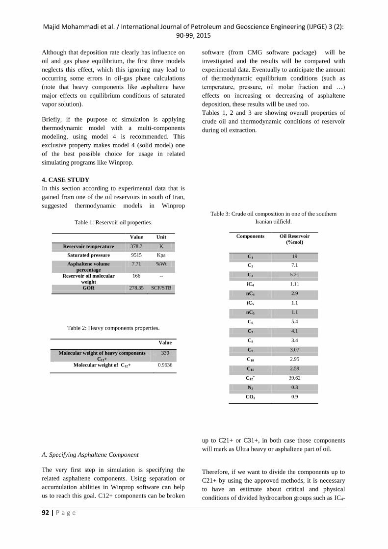
away after the bubble pressure. Figure 2 shows App
diagram for broken components of oil up to C31+.
After comparing the diagram with experimental data,
we realize that unlike the previous figure, in this case,
there is a good agreement between APP diagram
and experimental data after the bubble pressure while
this agreement is almost vanished for lower pressure
than bubble pressure.
Table 6: Experimental data for asphaltene deposition.
Asphaltene Deposition
(Wt%)
Pressure (Kpa)
2.71 6895
3.21 8963
2.86 13789
1.96 20684
Fig. 1: APP diagram after lumping to C21+.
Majid Mohammadi et al. / International Journal of Petroleum and Geoscience Engineering (IJPGE) 3 (2): 90-99, 2015
95 | P a g e
Fig. 2: APP diagram after lumping to C31+.
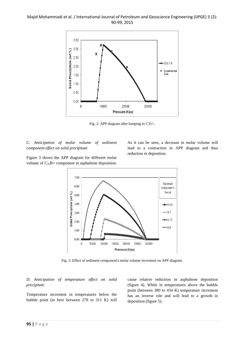
C. Anticipation of molar volume of sediment
component effect on solid precipitate
Figure 3 shows the APP diagram for different molar
volume of C31B+ component in asphaltene deposition.
As it can be seen, a decrease in molar volume will
lead to a contraction in APP diagram and thus
reduction in deposition.
Fig. 3: Effect of sediment component's molar volume increment on APP diagram.
D. Anticipation of temperature effect on solid
precipitate
Temperature increment in temperatures below the
bubble point (in here between 278 to 311 K) will
cause relative reduction in asphaltene deposition
(figure 4). While in temperatures above the bubble
point (between 380 to 434 K) temperature increment
has an inverse role and will lead to a growth in
deposition (figure 5).

Majid Mohammadi et al. / International Journal of Petroleum and Geoscience Engineering (IJPGE) 3 (2): 90-99, 2015
96 | P a g e
Fig. 4: Temperature increment (278-311 K) effect on APP diagram.
Fig. 5: Temperature increment (380-434 K) effect on APP diagram.
E. Anticipation of solvent gas injection effect on solid
precipitate
In this section, injection effect of different and
common gaseous solvents (that usually are being used
for enhanced oil recovery from reservoirs) on amount
of asphaltene deposition changes in APP diagrams
will be investigated. The major pure gases that their
effects (in various volumes) on amount of deposition
will be studied, are CO2 and N2. First with regards to
injected gas data, changes mode of asphaltene
deposition per different injected molar parts toward
extracted crude oil will be investigated. These data are
listed in table 7. It must be pointed out that majority
part of returned gas to the oil mixture are contain of
light hydrocarbon components such as C1, C2, and C3
than components like N2 and CO2. Figure 6 shows the
related APP diagram which according to that, per
pressures below bubble point, amount of increment in
deposition, during increase of molar volume of
injected gas are much lower than pressures above
bubble point. Moreover, higher molar fraction of
injected gas will lead to a sharp increase in asphaltene
deposition.

Majid Mohammadi et al. / International Journal of Petroleum and Geoscience Engineering (IJPGE) 3 (2): 90-99, 2015
97 | P a g e
Table 7: Sample injected gas compositions.
Component Injected gas
(%mol)
N2 0.79
CO2 2.49
C1 50.6
C2 18.45
C3 12.72
iC4 2.17
nC4 6.26
iC5 1.9
nC5 2.14
C6 1.77
C7 0.64
C8 0.07
Fig. 6: Effect of injected gas (in table 7) on APP diagram.
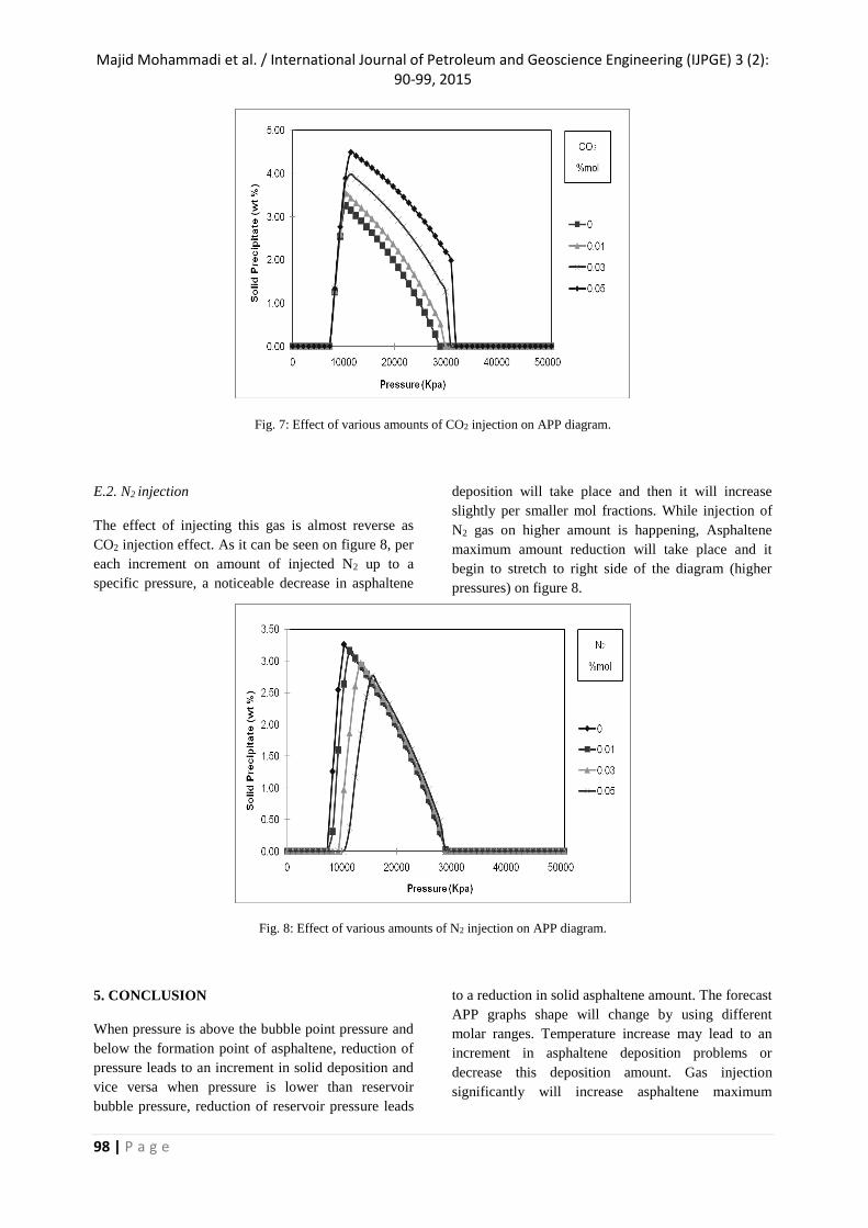
E.1. CO2 injection
Effect of CO2 injection on APP diagram is indicated
on figure 7. A very small increase in deposition
increment before the bubble pressure is detectable
while on pressures above the bubble point increase in
deposition during injection even in low amounts of
CO2 is relatively high.
Majid Mohammadi et al. / International Journal of Petroleum and Geoscience Engineering (IJPGE) 3 (2): 90-99, 2015
98 | P a g e
Fig. 7: Effect of various amounts of CO2 injection on APP diagram.
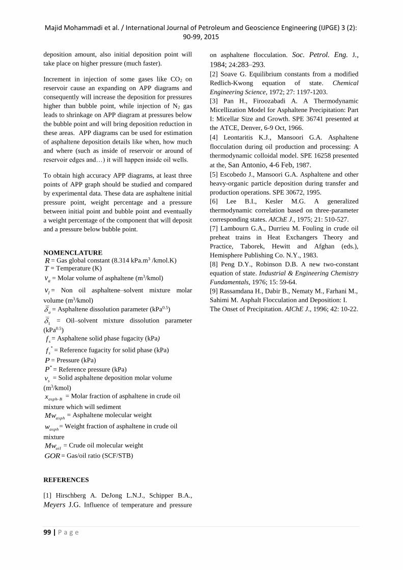
E.2. N2 injection
The effect of injecting this gas is almost reverse as
CO2 injection effect. As it can be seen on figure 8, per
each increment on amount of injected N2 up to a
specific pressure, a noticeable decrease in asphaltene
deposition will take place and then it will increase
slightly per smaller mol fractions. While injection of
N2 gas on higher amount is happening, Asphaltene
maximum amount reduction will take place and it
begin to stretch to right side of the diagram (higher
pressures) on figure 8.
Fig. 8: Effect of various amounts of N2 injection on APP diagram.
5. CONCLUSION
When pressure is above the bubble point pressure and
below the formation point of asphaltene, reduction of
pressure leads to an increment in solid deposition and
vice versa when pressure is lower than reservoir
bubble pressure, reduction of reservoir pressure leads
to a reduction in solid asphaltene amount. The forecast
APP graphs shape will change by using different
molar ranges. Temperature increase may lead to an
increment in asphaltene deposition problems or
decrease this deposition amount. Gas injection
significantly will increase asphaltene maximum
Majid Mohammadi et al. / International Journal of Petroleum and Geoscience Engineering (IJPGE) 3 (2): 90-99, 2015
99 | P a g e
deposition amount, also initial deposition point will
take place on higher pressure (much faster).
Increment in injection of some gases like CO2 on
reservoir cause an expanding on APP diagrams and
consequently will increase the deposition for pressures
higher than bubble point, while injection of N2 gas
leads to shrinkage on APP diagram at pressures below
the bubble point and will bring deposition reduction in
these areas. APP diagrams can be used for estimation
of asphaltene deposition details like when, how much
and where (such as inside of reservoir or around of
reservoir edges and…) it will happen inside oil wells.
To obtain high accuracy APP diagrams, at least three
points of APP graph should be studied and compared
by experimental data. These data are asphaltene initial
pressure point, weight percentage and a pressure
between initial point and bubble point and eventually
a weight percentage of the component that will deposit
and a pressure below bubble point.
NOMENCLATURE
R = Gas global constant (8.314 kPa.m3 /kmol.K)
T = Temperature (K)
av = Molar volume of asphaltene (m3/kmol)
lv = Non oil asphaltene–solvent mixture molar
volume (m3/kmol)
a = Asphaltene dissolution parameter (kPa0.5)
1 = Oil–solvent mixture dissolution parameter
(kPa0.5)
sf = Asphaltene solid phase fugacity (kPa)
*
sf = Reference fugacity for solid phase (kPa)
P = Pressure (kPa) *P = Reference pressure (kPa)
sv = Solid asphaltene deposition molar volume
(m3/kmol)
Basphx = Molar fraction of asphaltene in crude oil
mixture which will sediment
asphMw = Asphaltene molecular weight
asphw = Weight fraction of asphaltene in crude oil
mixture
oilMw = Crude oil molecular weight
GOR = Gas/oil ratio (SCF/STB)
REFERENCES
[1] Hirschberg A. DeJong L.N.J., Schipper B.A.,
Meyers J.G. Influence of temperature and pressure
on asphaltene flocculation. Soc. Petrol. Eng. J.,
1984; 24:283–293.
[2] Soave G. Equilibrium constants from a modified
Redlich-Kwong equation of state. Chemical
Engineering Science, 1972; 27: 1197-1203.
[3] Pan H., Firoozabadi A. A Thermodynamic
Micellization Model for Asphaltene Precipitation: Part
I: Micellar Size and Growth. SPE 36741 presented at
the ATCE, Denver, 6-9 Oct, 1966.
[4] Leontaritis K.J., Mansoori G.A. Asphaltene
flocculation during oil production and processing: A
thermodynamic colloidal model. SPE 16258 presented
at the, San Antonio, 4-6 Feb, 1987.
[5] Escobedo J., Mansoori G.A. Asphaltene and other
heavy-organic particle deposition during transfer and
production operations. SPE 30672, 1995.
[6] Lee B.I., Kesler M.G. A generalized
thermodynamic correlation based on three‐parameter
corresponding states. AIChE J., 1975; 21: 510-527.
[7] Lambourn G.A., Durrieu M. Fouling in crude oil
preheat trains in Heat Exchangers Theory and
Practice, Taborek, Hewitt and Afghan (eds.),
Hemisphere Publishing Co. N.Y., 1983.
[8] Peng D.Y., Robinson D.B. A new two-constant
equation of state. Industrial & Engineering Chemistry
Fundamentals, 1976; 15: 59-64.
[9] Rassamdana H., Dabir B., Nematy M., Farhani M.,
Sahimi M. Asphalt Flocculation and Deposition: I.
The Onset of Precipitation. AIChE J., 1996; 42: 10-22.


