

General rights Copyright and moral rights for the publications made accessible in the public portal are retained by the authors and/or other copyright owners and it is a condition of accessing publications that users recognise and abide by the legal requirements associated with these rights.
• Users may download and print one copy of any publication from the public portal for the purpose of private study or research. • You may not further distribute the material or use it for any profit-making activity or commercial gain • You may freely distribute the URL identifying the publication in the public portal
If you believe that this document breaches copyright please contact us providing details, and we will remove access to the work immediately and investigate your claim.
Downloaded from orbit.dtu.dk on: Dec 20, 2017
Eigenbeamforming array systems for sound source localization
Tiana Roig, Elisabet; Jacobsen, Finn; Jeong, Cheol-Ho; Agerkvist, Finn T.
Publication date:2014
Document VersionPublisher's PDF, also known as Version of record
Link back to DTU Orbit
Citation (APA):Tiana Roig, E., Jacobsen, F., Jeong, C-H., & Agerkvist, F. T. (2014). Eigenbeamforming array systems for soundsource localization. Technical University of Denmark, Department of Electrical Engineering.

Elisabet Tiana Roig
Eigenbeamforming array systems for sound source localization PhD thesis, November 2014


Eigenbeamforming array systems
for sound source localization
PhD thesis by
Elisabet Tiana Roig
Technical University of Denmark
2014
This thesis was submitted to the Technical University of Denmark (DTU) as partial
fulfillment of the requirements for the degree of Doctor of Philosophy (PhD) in Elec-
tronics and Communication. The work presented in this thesis was completed between
October 1, 2010 and August 1, 2014 at Acoustic Technology, Department of Electrical
Engineering, DTU, under the supervision of Associate Professor Finn Jacobsen, until
June of 2013, and Associate Professors Cheol-Ho Jeong and Finn T. Agerkvist, from
March of 2013 to the end. The project was funded by the Department of Electrical
Engineering at DTU.
Cover illustration: Circular microphone array mounted on
a rigid sphere, by Elisabet Tiana-Roig
Department of Electrical Engineering
Technical University of Denmark
DK-2800 KONGENS LYNGBY, Denmark
Printed in Denmark by Rosendahls - Schultz Grafisk a/s
c© 2014 Elisabet Tiana Roig
No part of this publication may be reproduced or transmitted in any form or by any
means, electronic or mechanical, including photocopy, recording, or any information
storage and retrieval system, without permission in writing from the author.

In memory of Finn Jacobsen.
I al Toni, el meu far,
i al Quim, la meva llum.


Abstract
Microphone array technology has been widely used for the localization of sound
sources. In particular, beamforming is a well-established signal processing method that
maps the position of acoustic sources by steering the array transducers toward different
directions electronically.
The present PhD study aims at enhancing the performance of uniform circular ar-
rays, and to a lesser extent, spherical arrays, for two- and three-dimensional localization
problems, respectively. These array geometries allow to perform eigenbeamforming,
beamforming based on the decomposition of the sound field in a series of orthogonal
functions. In this work, eigenbeamforming is particularly developed to improve the
performance of circular arrays at low frequencies. Compared to conventional delay-
and-sum beamforming, the proposed technique, named circular harmonics beamform-
ing, provides a better resolution at the expense of being more vulnerable to noise. A
simple way to further improve the array performance is to flush-mount the transducers
on a rigid scatterer. For a circular array, an ideal solution is a rigid cylindrical scat-
terer of infinite length. Due to its impracticality, the use of a rigid spherical scatterer is
recommended instead.
A better visualization in the entire frequency range can be achieved with deconvo-
lution methods, as they allow the recovery of the sound source distribution from a given
beamformed map. Three efficient methods based on spectral procedures, originally
conceived for planar-sparse arrays, are adapted to circular arrays. They rely on the fact
that uniform circular arrays present an azimuthal response that is rather independent on
the focusing direction.
Finally, a method based on the combination of beamforming and acoustic holog-
raphy is introduced for both circular and spherical arrays. This new approach, also
expressible in terms of eigenbeamforming, extends the frequency range of operation of
conventional delay-and-sum beamforming toward the low frequencies.
Keywords: uniform circular arrays, spherical arrays, circular harmonics beamforming,
deconvolution methods, spherical harmonics beamforming, holographic virtual arrays
v

Resume
Mikrofon-array-teknologi har været meget anvendt til lokalisering af lydkilder. Navnlig
beamforming er en veletableret signalbehandlingsmetode, som kortlægger placeringen
af akustiske kilder ved elektronisk at styre array transducere mod forskellige retninger.
Dette Ph.d.-projekt stræber efter at forbedre præstationen af ensartede cirkulære
array-systemer, og i mindre grad sfæriske arrays, for hhv. to- og tredimensionale
lokaliseringsproblemer. Disse array-geometrier giver mulighed for at udføre eigen-
beamforming, dvs. beamforming baseret pa dekompositionen af lydfeltet i en række
ortogonale funktioner. I dette arbejde er eigenbeamforming specielt udviklet for at
forbedre præstationen af cirkulære arrays ved lave frekvenser. Sammenlignet med kon-
ventionel delay-and-sum beamforming giver den foreslaede teknik, kaldet circular har-
monics beamformning, en bedre opløsning pa bekostning af at være mere sarbar over
for støj. En enkel made til yderligere at forbedre array-præstationen er at placering
mikrofonerne pa overfladen af en hard scatterer. For et cirkulært array er en ideel
løsning en hard cylindrisk scatterer af uendelig længde. Pa grund af vanskeligheder
ved implementeringen anbefales en hard sfærisk scatterer i stedet for.
En bedre visualisering i hele frekvensomradet kan opnas med deconvolution-
metoder, da de tillader gendannelse af lydkilders distribution fra et givet beamformed
kort. Tre effektive metoder, baseret pa spektrale procedurer, der oprindeligt er udtænkt
til plane, sparse arrays, er tilpasset cirkulære arrays. De er afhængige af det faktum,
at ensartede cirkulære arrays viser et azimut respons, der er temmelig uafhængig af
fokuseringen retning.
Endelig indføres en metode, der bygger pa en kombination af beamforming og
akustisk holografi, for bade cirkulære og sfæriske arrays. Denne nye fremgangsmade,
som ogsa kan udtrykkes i form af eigenbeamforming, udvider frekvensomradet for bru-
gen af konventionel delay-and-sum beamforming mod de lave frekvenser.
Nøgleord: ensartede cirkulære arrays, sfæriske arrays, circular harmonics beamform-
ing, spherical harmonics beamforming, deconvolution-metoder, holografiske virtuelle
arrays
vii

Acknowledgments
I would like to dedicate these first lines to pay my deepest homage to my supervisor,
Finn Jacobsen. This work would have not been possible without his teachings, his
generous dedication, and his wise advice. I will always admire him for being committed
to his work and to his students until the very end of his life. Moving the project forward
without him has been extremely tough. However, his legacy has given me strength and
has accompanied me every single day until the end of the project. His memory will
always live within me.
I will never forget the support of the other professors of the group, Cheol-Ho Jeong,
Finn T. Agerkvist, and Jonas Brunskog, when Finn Jacobsen was forced to step aside
a year and a half ago. In particular, I would like to thank Cheol-Ho for taking over the
main supervision, and for doing it with motivation and efficiency. I am also extremely
grateful to Efren Fernandez-Grande for his great support, guidance, and help, all the
way through.
All my colleagues, former colleagues, and friends, at the ‘House of Acoustics’
have contributed immensely to my personal and professional time at DTU. In particu-
lar, I would like to express my gratitude to Jørgen Rasmussen and Tom A. Petersen for
their help with the equipment and the experimental work, and to Nadia J. Larsen for
her help with administrative tasks and for her empathy. I am very grateful to Aggeliki
Xenaki, Oliver Lylloff, and Marco Ottink for letting me participate in their Master’s the-
ses; I have really learned a lot from you. Many thanks to Salvador Barrera Figueroa for
his advice and also for his subtle way of cheering me up. Thanks to Marton Marschall
for his Matlab code and for the fruitful discussions regarding spherical arrays. I am
also very grateful to Torsten Dau for his experienced advice during a complicated peer-
review process of one of the articles. Special thanks to my wonderful office mates,
Joe Jensen, Gerd Marbjerg, and Alba Granados, for creating a fantastic working atmo-
sphere. Joe, thanks for your permanent good mood, and your (almost perfect) musical
taste. Gerd, Alba, I have really enjoyed this short, but intense, time together in our
particular fortress. Without your support in the last months, this would have been a lot
harder.
ix
x Acknowledgments
I am very grateful to Karim Haddad and Jørgen Hald from Bruel & Kjær for lending
me equipment for the experiments, and for very inspiring discussions.
Thanks to Daniel Fernandez-Comesana from Microflown Technologies for inviting
me to participate in one of his articles.
I would also like to thank an anonymous reviewer of the Journal of the Acoustical
Society of America, whose valuable comments became the basis of one of the appen-
dices of this dissertation.
I am indebted to my family and friends for encouraging me countless times, espe-
cially when I needed it most. I deeply thank my mom, my brother Eduard, my dad,
Piluca, my sister Vicky, my grandma Carme, in short, all my closest family, for their
love and support in all my pursuits. This PhD degree is an accomplishment that belongs
to all of them. It also belongs to my dear grandpa Guillem, who left us a few months
after the beginning of the project, and to my son Quim, who, born in the course of this
project, has been a great source of happiness. Finally, my most sincere gratitude to
Toni Torras Rosell. Without your precious and enthusiastic contribution to the papers,
your guidance on the dissertation, and your faith in me, this would have simply been
impossible. Thanks for being always there, for the dedication to our family, and for
your love.

Contents
List of acronyms xiii
List of symbols xv
Notations and conventions xix
1 Introduction 1
1.1 Scope of the thesis . . . . . . . . . . . . . . . . . . . . . . . . . . . . 2
1.2 A brief overview on acoustic array systems . . . . . . . . . . . . . . . 3
1.2.1 Beamforming techniques . . . . . . . . . . . . . . . . . . . . . 3
1.2.2 Other array techniques . . . . . . . . . . . . . . . . . . . . . . 4
1.2.3 Array layouts . . . . . . . . . . . . . . . . . . . . . . . . . . . 5
1.3 Structure of the thesis . . . . . . . . . . . . . . . . . . . . . . . . . . . 7
2 Basic beamforming methods 11
2.1 Delay-and-sum beamforming . . . . . . . . . . . . . . . . . . . . . . . 11
2.1.1 Uniform linear array . . . . . . . . . . . . . . . . . . . . . . . 17
2.1.2 Uniform circular array . . . . . . . . . . . . . . . . . . . . . . 21
2.1.3 Spherical array . . . . . . . . . . . . . . . . . . . . . . . . . . 25
2.2 Performance indicators . . . . . . . . . . . . . . . . . . . . . . . . . . 26
3 Eigenbeamforming 33
3.1 Introduction . . . . . . . . . . . . . . . . . . . . . . . . . . . . . . . . 33
3.1.1 Eigenbeamforming for circular arrays . . . . . . . . . . . . . . 34
xi

xii Contents
3.1.2 Eigenbeamforming for spherical arrays . . . . . . . . . . . . . 38
3.2 Papers A and B . . . . . . . . . . . . . . . . . . . . . . . . . . . . . . 40
3.2.1 Synopsis . . . . . . . . . . . . . . . . . . . . . . . . . . . . . 40
3.2.2 Related work . . . . . . . . . . . . . . . . . . . . . . . . . . . 40
3.2.3 Discussion . . . . . . . . . . . . . . . . . . . . . . . . . . . . 41
4 Deconvolution methods 45
4.1 Introduction . . . . . . . . . . . . . . . . . . . . . . . . . . . . . . . . 45
4.2 Paper C . . . . . . . . . . . . . . . . . . . . . . . . . . . . . . . . . . 48
4.2.1 Synopsis . . . . . . . . . . . . . . . . . . . . . . . . . . . . . 48
4.2.2 Related work . . . . . . . . . . . . . . . . . . . . . . . . . . . 49
4.2.3 Discussion . . . . . . . . . . . . . . . . . . . . . . . . . . . . 49
5 Beamforming with holographic virtual arrays 53
5.1 Introduction . . . . . . . . . . . . . . . . . . . . . . . . . . . . . . . . 53
5.2 Papers D and E . . . . . . . . . . . . . . . . . . . . . . . . . . . . . . 55
5.2.1 Synopsis . . . . . . . . . . . . . . . . . . . . . . . . . . . . . 55
5.2.2 Related work . . . . . . . . . . . . . . . . . . . . . . . . . . . 55
5.2.3 Discussion . . . . . . . . . . . . . . . . . . . . . . . . . . . . 56
6 Conclusions 59
6.1 Summary and conclusions . . . . . . . . . . . . . . . . . . . . . . . . 59
6.2 Future work . . . . . . . . . . . . . . . . . . . . . . . . . . . . . . . . 61
A Insight into circular harmonics beamforming 63
B Acoustic holography with uniform circular arrays 67
B.1 Open array . . . . . . . . . . . . . . . . . . . . . . . . . . . . . . . . 67
B.2 Rigid cylindrical scatterer of infinite length . . . . . . . . . . . . . . . 68
B.3 Rigid spherical scatterer . . . . . . . . . . . . . . . . . . . . . . . . . 70
Bibliography 73
Papers A-E 83

List of acronyms
CMF Covariance matrix fitting
DAMAS Deconvolution approach for the mapping of acoustic sources
DI Directivity index
ESPRIT Estimation of signal parameters via rotational invariance techniques
FFT Fast Fourier transform
FFT-NNLS Fourier-based non-negative least squares
FISTA Fast iterative shrinkage-thresholding algorithm
GSC Generalized sidelobe canceler
ISCA Iterative sidelobe cleaner algorithm
MACS Mapping of acoustic sources
MEMS Microelectromechanical systems
MSL Maximum sidelobe level
MUSIC Multiple signal classification
NAH Near-field acoustic holography
SHARP Spherical harmonics angularly resolved pressure
SNR Signal-to-noise ratio
SONAH Statistical optimized near-field acoustic holography
WNG White noise gain
2D Two-dimensional
3D Three-dimensional
xiii


List of symbols
A Amplitude of the acoustic wave
An Expansion coefficient of order n
b Beamformer output
b Beamformer power response expressed as a vector
C Cross-spectral matrix
Cn nth Fourier coefficient obtained with a continuous circular aperture
Cn nth Fourier coefficient estimated with a circular array
Cmn mnth Fourier coefficient obtained with a continuous spherical aperture
Cmn mnth Fourier coefficient estimated with a spherical array
c Speed of sound in the medium of propagation
cmn mnth element of the cross-spectral matrix C
d Sensor spacing of a linear array
dn Constant associated to the nth order in eigenbeamforming
F Direct FFT
F−1 Inverse FFT
f Frequency
G Grid
H Point-spread function
H Point-spread function matrix
H(1)n Hankel function of the first kind and order n
h(1)n Spherical Hankel function of the first kind and order n
Jn Bessel function of the first kind and order n
j Imaginary number(√−1
)jn Spherical Bessel function of the first kind and order n
k Wavenumber
xv
xvi List of symbols
k Wavenumber vector
ki Wavenumber vector of an incident wave
M Number of array sensors
N Number of orders in eigenbeamforming
Nv Number of orders in eigenbeamforming with a holographic virtual array
Pmn Associated Legendre function of order m and degree n
pm Sound pressure captured at the mth array sensor
p Sound pressure
Qn Baffle condition function
R Radius of a circular/spherical array of sensors
Rv Radius of a holographic virtual array
r Position vector
rm Position of the mth array sensor
s Spatial source power distribution
s Spatial source power distribution vector
t Time
Un Chebyshev polynomial of the second kind of degree n
W Array pattern
wm Weighting of the mth array sensor
wn Weighting of the nth harmonic order
Y mn Spherical harmonic of order n and degree m
αm Integration factor of the mth sensor of a circular/spherical array
δ Delta function
δnν Kronecker delta function
ϕ Azimuth angle, from 0 to 2π
ϕl Azimuth angle of the array looking direction, from 0 to 2π
ϕm Azimuth angle of the mth array sensor, from 0 to 2π
ϕs Azimuth angle of a sound source, from 0 to 2π
κ Array’s steering vector
λ Wavelength
θ Polar angle, from 0 to π
θm Polar angle of the mth array sensor, from 0 to π
θs Polar angle of a sound source, from 0 to π
ϑ Polar angle, from −π to π
xvii
ϑs Polar angle of a sound source, from −π to π
τm Delay applied to the mth array sensor
ω Angular frequency

Notations and conventions
Conventions
• The convention e−jωt is considered in the entire manuscript. Hence, a progres-
sive plane wave is of the form ej(k · r−ωt).
• Vectors are denoted by boldface lowercase characters, e.g., a.
• Matrices are denoted by boldface uppercase characters, e.g., A.
• Unit vectors are denoted by boldface lowercase characters with a hat, e.g., a.
Mathematical operations
( · )∗ Complex conjugate of the argument
| · | Absolute value of the argument
� · � Ceiling function of the argument
‖ · ‖2 2-norm of the argument
xix


Chapter 1
Introduction
A problem of practical importance when dealing with acoustic measurements is to esti-
mate the directions from which sound waves arrive to the measurement point. While a
single microphone cannot provide this information, as microphones are only capable of
measuring the sound pressure at that specific point, combination of simultaneous sig-
nals from an array of microphones makes it possible to filter the sound in space and,
thus, achieve directionality. With proper signal processing, array systems can focus into
a particular direction, to enhance the signals arriving from there, and attenuate those
from other directions. This idea was explored for the first time in 1976, when Billings-
ley and Kinns introduced the acoustic telescope, a system that was able to localize the
main contributions of jet engines in real-time [1]. This work laid the foundations of
beamforming, which soon became popular among the acoustic community, giving rise
to numerous studies not only for sound source localization purposes, but also for signal
enhancement and spatial filtering. Nowadays beamforming is an essential tool widely
used in the industry for all sorts of applications, such as vehicle assessment, computer
games and surveillance, among others. Depending on the application, the most ad-
equate processing techniques and array geometries vary. Generally, beamforming is
based on measurements in the far field of the sources so that the waves have become
planar at the array position. However, it should be noticed that near-field beamforming
is also possible. Readers interested in the history of beamforming are addressed to the
concise monograph by Michel, Ref. [2].
An ideal sound source localization system should present a delta function on the
focusing direction and nulls elsewhere. However, beamforming presents two inher-
ent limitations; firstly, an imperfect resolution on the focusing direction, due to a main
1
2 1. Introduction
beam instead of a delta function, and secondly, the appearance of sidelobes in directions
other than the focusing direction. Moreover, the array response is frequency dependent.
The frequency range of operation of an array is determined, at low frequencies, by
the dimensions of the array, and by the microphone spacing, at high frequencies. The
larger the array, the better the performance at low frequencies, whereas the closer the
microphones, the better at high frequencies. However, the dimensions of the array and
the number of microphones are usually limited by practical issues, such as the maneu-
verability of the array and the overall cost of the equipment. Therefore, dealing with
broadband sources poses some challenges. In the almost 40 years of development of
acoustic array technology, numerous beamforming algorithms, as well as array geome-
tries, have been suggested to improve the overall performance of array systems.
1.1 Scope of the thesis
The present thesis deals with circular and spherical arrays of microphones, to a lesser
extent, for localization of sound sources in 2-dimensional (2D) and 3-dimensional (3D)
sound fields, respectively. While spherical arrays have been examined widely in the
last decade for speech enhancement and sound source localization purposes, less liter-
ature has been devoted to circular arrays. This geometry is particularly interesting for
scenarios where sources placed in the far field are distributed 360◦ around the array.
That is, for instance, the case of many outdoor measurements for environmental noise
identification, in which reflections from the ground are sufficiently attenuated, and also
the case of measurements in rooms where floors and ceilings are acoustically treated
to reduce reflections. One of the main applications involving rooms is conferencing,
a scenario that requires beamforming in real-time; see, e.g., Ref. [3]. By contrast,
for environmental noise purposes, measurements can be often post-processed at a later
stage, which allows the application of more sophisticated algorithms that require a high
computational load. The primary goal of the present thesis is to suggest and examine
alternatives to the traditional methods for enhancing the performance of these array
geometries for sound source localization purposes.
It should be noticed that, throughout this dissertation, it is assumed that the acoustic
sources are static, placed in the far field of the array, and not coherent. It is also assumed
that all the array transducers have the same characteristics and are omnidirectional.

1.2 A brief overview on acoustic array systems 3
1.2 A brief overview on acoustic array systems
1.2.1 Beamforming techniques
Beamforming techniques are generally classified in two groups: fixed beamforming
and adaptive beamforming. Fixed beamforming algorithms are data-independent, that
is, all signals are treated in the same manner without taking into account their individual
properties. The simplest method is delay-and-sum beamforming, which is addressed in
Chapter 2. Another example is filter-and-sum beamforming, based on linearly filtering
the signals prior to applying delay-and-sum; see, e.g., Ref. [4]. Filtering helps removing
disturbances, such as out-of-band noise. A new and specially attractive technique for
its simplicity is functional beamforming [5]. This method that results from modifying
delay-and-sum beamforming in the frequency domain offers a much higher dynamic
range than other beamforming techniques. However, it is very sensitive to microphone
positioning errors.
On the other hand, adaptive beamforming methods are data-dependent, that is, their
parameters follow from statistical observations in the captured signals. As a result,
their performance exceeds that of fixed beamforming techniques, at the expense of be-
ing more complex to implement and more sensitive to sensor calibration errors [4].
Furthermore, in the presence of coherent sources, most methods fail dramatically. Usu-
ally, adaptive techniques rely on narrow-band signals. Several methods are based on
solving a constrained mean-squared optimization problem. That is, for instance, the
case of the generalized sidelobe canceler (GSC) [6], which basically consists of a fixed
beamformer, a blocking matrix, and an interference canceler. The fixed beamformer
is steered to the desired direction, while the blocking matrix blocks any signal coming
from that direction so that only noise signals from undesired directions pass through. By
means of an adaptive algorithm the unwanted signals are emphasized and finally they
are subtracted from the fixed beamformer output. Another type of adaptive techniques,
the so-called high-resolution spectral estimation techniques, are derived from parame-
ter estimation theory. One such method is the multiple signal classification (MUSIC),
which, based on eigenanalysis, relies on the orthogonality between the signals subspace
and the noise subspace to improve the quality of the signals [7]. Adaptive methods are
out of the scope in this dissertation. Readers interested in adaptive beamforming are,
for instance, referred to Chapter 7 in Ref. [4] and Chapter 5 in Ref. [8].
Although most beamforming techniques are in essence independent of the array
4 1. Introduction
geometry, there is a group of methods conceived for ‘closed’ arrays, such as circular
and spherical arrays, known as eigenbeamforming. Eignebeamforming relies on the
decomposition of the sound field captured with the array in a series of harmonics, which
adds more features compared to traditional beamforming. Fixed eigenbeamforming
methods are addressed in Chapter 3.
In the last decade, a group of inverse methods, generally referred to as deconvo-
lution methods, has become of interest, as they allow to visualize sound sources with
more accuracy than beamforming methods, and even determine their levels. However,
the main limitation is that they are computationally expensive, as they are based on
iterative algorithms. An overview of these methods is given in Chapter 4.
It should be noted that beamforming can be applied also to moving sources. Since
in the present study only static sources are considered, the reader is addressed to,
e.g., Chapter 8 in Ref. [4] for a basic introduction to tracking problems.
1.2.2 Other array techniques
Besides beamforming, there are other sound visualization techniques that rely on ar-
ray measurements. The most relevant one is acoustic holography, a well-established
method that aims at reconstructing sound fields quantitatively. By means of measure-
ments in a 2D surface (the array), the entire sound field, sound pressure, particle ve-
locity, and sound intensity, can be reconstructed in a 3D space. Acoustic holography
and beamforming are complementary techniques, as acoustic holography is generally
preferred for near-field measurements, such as in near-field acoustic holography (NAH)
[9, 10], whereas beamforming is more adequate for the far-field case. Moreover, acous-
tic holography handles better coherent than incoherent sources, which contrasts with the
opposite behavior of beamforming. In most applications, acoustic holography serves to
describe the radiation characteristics of the source under analysis.
Array technology is also used for blind source separation, although an array layout
is not strictly necessary. As the name suggests, blind source separation is a sound source
identification method that intends to simultaneously recover signals from independent
sources without requiring any information on their locations. The main limitation of the
method is that it fails when there are more sources than sensors. Blind source separation
is not addressed in this thesis. Readers interested in a thorough comparison between

1.2 A brief overview on acoustic array systems 5
blind source separation and beamforming in the time-domain (for speech purposes) are
referred to Ref. [11].
1.2.3 Array layouts
Traditionally, beamforming has been carried out mostly with planar-sparse arrays. The
simplest configuration is the rectangular grid of elements. However, due to the peri-
odical placement of the sensors, severe sampling error, in the form of aliasing, occurs
above the frequency where the spatial Nyquist sampling criterion is not fulfilled. This
causes a sudden increase in level of the sidelobes, which become replicas of the main
lobe in unwanted directions in the worst case. This is addressed in Chapter 2. This
characteristic prevents this geometry from being generally used for beamforming pur-
poses. Contrarily, rectangular arrays, with one or two parallel layers, are typically used
for NAH.
Planar irregular arrays are usually preferred for beamforming over regular arrays,
because they do not exhibit an abrupt aliasing pattern. The effect of an aperiodical spa-
tial sampling is a smooth increase in the level of the sidelobes, which leads to a wider
frequency range of operation toward high frequencies [12]. Typical irregular arrays
used for aeroacoustic purposes are based on spirals, such as the equiangular or loga-
rithmic spiral array with one or more arms [13, 14]. Some other irregular layouts result
from optimization processes that determine the position of the sensors that ensures the
best possible level of the sidelobes for the frequency range of interest [12]. For some
applications, such as wind tunnel measurements, it is convenient to flush-mount the
array microphones on a wall or a baffle so that the array structure does not alter the
aerodynamic environment. References [12] and [15] examine various planar irregular
arrays in detail.
Spherical arrays are also widely used for beamforming [16], as well as for acoustic
holography [17], whereas circular arrays are less common [18], especially for holog-
raphy. Generally, spherical and circular arrays used for sound source localization are
shift-invariant, that is, the output pattern is independent of the focusing direction so that
the system is equally fair in all directions. One way to achieve this characteristic is by
keeping a constant microphone spacing all over the array. That is, for instance, the case
of a uniform circular array [19]. This interesting feature cannot be achieved with linear
or planar-sparse arrays.

6 1. Introduction
On the other hand, spherical arrays with non-uniform spacing have also been inves-
tigated, e.g., in Ref. [20]. That is, for instance, the case of a rigid spherical array with
the sensors placed in horizontal rings with a higher density of sensors on the equator
of the sphere suggested in Refs. [21–23] to enhance the horizontal spatial resolution
over other directions. This array is suitable for 3D recordings that can afterwards be
used to create virtual environments for hearing instrument testing and psychoacoustic
purposes via a high-order or a mixed-order Ambisonics loudspeaker system [24]. Cir-
cular arrays with a non-uniform spacing are rather unusual. An example can though be
found in Ref. [25], where the angular position of the array sensors is determined by the
golden-ratio.
Variations of the circular and spherical geometries are also found in the literature.
For example, Refs. [26, 27] suggest a dual-radius spherical array for beamforming and
for NAH that consists of an open spherical array with a smaller spherical array mounted
on a baffle in its interior, whereas Ref. [28] introduces an open dual-radius spherical
array. Similarly, Refs. [29, 30] examine systems that consist of concentric uniform
circular arrays of different radius. For beamforming purposes on a half 3D acoustic
scenario, Ref. [31] suggests a baffled hemispherical microphone array that makes use
of the image source principle.
To achieve a rather constant pattern in the entire frequency range of interest, some
arrays are conformed by subarrays, each being responsible for a certain frequency band.
Usually, this is approached with planar-sparse arrays [8, 32], although other configura-
tions are applicable to, such as the previous mentioned concentric circular and spherical
arrays. A wise solution to reduce the overall cost of the system is to share, when pos-
sible, array elements between different subarrays, giving rise to the concept of nested
arrays. The idea of using nested arrays, is, in fact, the essence of constant directiv-
ity beamforming, a fixed beamforming method based on applying filter-and-sum to the
the different nested arrays [8, 32]. The main drawback of this technique is that it is
impractical at low frequencies, as it requires extremely large arrays.
In the presence of stationary signals, ‘scanning arrays’ are alternatives to conven-
tional arrays. The procedure only requires two transducers: while one is kept at a
position that serves as a reference, the other is moved along a grid [33]. The main ad-
vantage is that the equipment required is obviously cheaper than a that of a conventional
array system. Besides, the method offers more flexibility in the sense that the scanning
area is not limited to a predefined grid of points. The main drawback, though, is that

1.3 Structure of the thesis 7
measurements are more time consuming. Based on this principle, a scanning array con-
sisting of a rotating microphone set-up is suggested to capture the acoustic behavior
of auditoriums in Ref. [34]. The data measured with the array, a large set of impulse
responses, is later used for creating virtual acoustic scenes with a 2D or 3D Ambisonics
loudspeaker system.
Most array systems assume that the sensors are completely omnidirectional. How-
ever, microphones with well-defined directivity patterns can also be used, provided that
all of them are of the same type and are oriented identically. In such a case, the transfer
function of the directive microphones must be taken into account for the beamform-
ing procedure [32]. Besides conventional microphones, pressure-velocity transducers,
e.g., Microflown PU probes [35], are progressively attracting interest. These transduc-
ers provide simultaneous measurements of pressure and particle velocity, which make
them particularly suitable for acoustic holography [36]. In fact, some NAH methods
rely on the combination of the two quantities to achieve an enhanced performance [37–
39].
Recently, a completely new approach for beamforming based on the acousto-optic
effect, i.e., the interaction between sound and light, has been introduced in Ref. [40].
Instead of using a discrete number of sensors as in conventional arrays, the proposed
acousto-optic beamformer senses the sound field with a laser beam in a continuous
manner so that spatial aliasing is totally avoided. So far, only an optical linear aperture
has been examined [41]. At the moment, the main drawback of this technique is that
the beamformer requires manual steering. However, this problem could be overcome
by developing an optical array.
1.3 Structure of the thesis
The present PhD thesis follows a paper-based format, that is, the main findings of the
PhD project are presented in a collection of articles elaborated in the course of the
project. It is important to emphasize that the articles represent the core of the thesis.
The dissertation is structured as follows: Chapter 2, Basic beamforming methods,
gives the basic concepts of beamforming required to follow the contributing papers.
Readers familiar with the topic can skip this chapter. Chapter 3, Eigenbeamforming,
Chapter 4, Deconvolution methods, and Chapter 5, Beamforming with holographic vir-
tual arrays, are devoted to the findings of the contributing articles. These chapters share

8 1. Introduction
the same structure: they begin with an introduction that intends to supplement, when
possible, the articles, followed by a synopsis of the articles, a survey on related work,
and a discussion of the findings. Unlike Chapter 2, Chapters 3 to 5 are kept deliber-
ately concise to minimize the repetition in content with the contributing papers. Since
these chapters are understood as a complement to the papers, the reader is advised to
read the papers before proceeding to the final chapter, Conclusions, which concludes
the work and suggests further investigations for the future. The thesis also includes two
appendices that supplement Chapter 3 and 5, respectively.
The contributing papers, five in total, are appended at the end. Three of them are
published in the Journal of the Acoustical Society of America, and the rest are published
in the proceedings of two relevant congresses. They are listed in the following:
Paper A E. Tiana-Roig, F. Jacobsen, and E. Fernandez-Grande, “Beamforming with
a circular microphone array for localization of environmental noise sources,” J.
Acoust. Soc. Am., vol. 128, no. 6, pp. 3535–3542, 2010.∗
Paper B E. Tiana-Roig, F. Jacobsen, and E. Fernandez-Grande, “Beamforming with
a circular array of microphones mounted on a rigid sphere (L),” J. Acoust. Soc.
Am., vol. 130, no. 3, pp. 1095–1098, 2011.
Paper C E. Tiana-Roig and F. Jacobsen, “Deconvolution for the localization of sound
sources using a circular microphone array”, J. Acoust. Soc. Am., vol. 134, no. 3,
pp. 2078–2089, 2013.
Paper D E. Tiana-Roig, A. Torras-Rosell, E. Fernandez-Grande, C.-H. Jeong, and
F. T. Agerkvist, “Towards an enhanced performance of uniform circular arrays
at low frequencies,” in Proc. of Inter-Noise 2013, Innsbruck, Austria, 2013.
Paper E E. Tiana-Roig, A. Torras-Rosell, E. Fernandez-Grande, C.-H. Jeong, and
F. T. Agerkvist, “Enhancing the beamforming map of spherical arrays at low fre-
quencies using acoustic holography,” in Proc. of BeBeC 2014, Berlin, Germany,
2014.
∗Paper A is based on the Master’s thesis by Elisabet Tiana Roig “Beamforming Techniques for environ-
mental noise”, Technical University of Denmark, 2009. The paper, written in 2010 during the application
process of the PhD project, is included as part of this PhD thesis as it led to the research topic of the project.

1.3 Structure of the thesis 9
Besides the aforementioned articles, the following articles were also produced in
the course of the PhD project:
1 E. Tiana-Roig and F. Jacobsen, “Acoustical source mapping based on deconvolution
approaches for circular microphone arrays,” in Proc. of Inter-Noise 2011, Osaka,
Japan, 2011.
2 Fernandez-Comesana, E. Fernandez-Grande, and E. Tiana-Roig, “A novel deconvo-
lution beamforming algorithm for virtual phased arrays”, in Proc. of Inter-Noise
2013, Innsbruck, Austria, 2013.
However, these articles are not explicitly mentioned in the thesis, as the contents of
Paper 1 overlap with Paper C and Paper 2 does not directly relate to the work done in
eigenbeamforming.

10 1. Introduction

Chapter 2
Basic beamforming methods
This chapter provides the basic knowledge required to comprehend the main contribu-
tions of the PhD project. The chapter begins with an introduction to classical beam-
forming theory. Two array geometries are examined in detail, the uniform linear array,
which serves to explain the basic concepts of beamforming, and the uniform circular
array as most contributing papers (Papers A to D) elaborate on this array configuration.
In addition, the case of a spherical array is touched upon, as paper E deals with this ge-
ometry. The chapter ends with a description of the measures of performance commonly
used to evaluate beamforming systems.
2.1 Delay-and-sum beamforming
Delay-and-sum beamforming is the oldest and simplest array signal processing algo-
rithm [4]. The principle behind this technique is shown in Fig. 2.1: in the presence of
a propagating wave, the signals captured by the microphones are delayed by a proper
amount before being added together, to strengthen the resulting signal with respect to
noise or waves propagating in other directions. The delays required to reinforce the
output signal correspond to the time it takes for the wave to propagate between micro-
phones so that, after applying the delays, the microphone signals are aligned in time.
Mathematically, delay-and-sum is formulated as
b(t, κ) =
M−1∑m=0
wmpm(t− τm(κ)), (2.1)
11

12 2. Basic beamforming methods
0
1
2
M − 1
+
pM−1(t)
p1(t)
p2(t)
w0p0(t− τ0)
b(t)
τ0
τ1
τ2
τM−1
wM−1pM−1(t− τM−1)
p0(t) w0
w1
w2
wM−1
Figure 2.1: Sketch of a delay-and-sum beamformer. The signals captured by the sensors are delayed (and
weighted) before adding them together.
originarray
rmκ
Figure 2.2: Array focused in the direction given by κ.
where M is the number of microphones, pm is the pressure measured with the mth
microphone, wm is its associated amplitude weighting, and τm(κ) is the delay applied
to the mth microphone required to focus the array in the direction given by κ depicted
in Fig. 2.2. The delays are given by
τm(κ) =κ · rm
c, (2.2)
where rm is the position vector of the mth microphone and c is the speed of sound in
the medium of propagation (approximately 343 m/s in air at 23◦C).
Assuming a plane wave that impinges on the array, the pressure captured by the
mth array microphone, expressed in complex notation, is
pm(t) = Aej(ki · rm−ωt), (2.3)
2.1 Delay-and-sum beamforming 13
ki
rm
originarray
plane
wave
main
lobe
sidelobes
κ
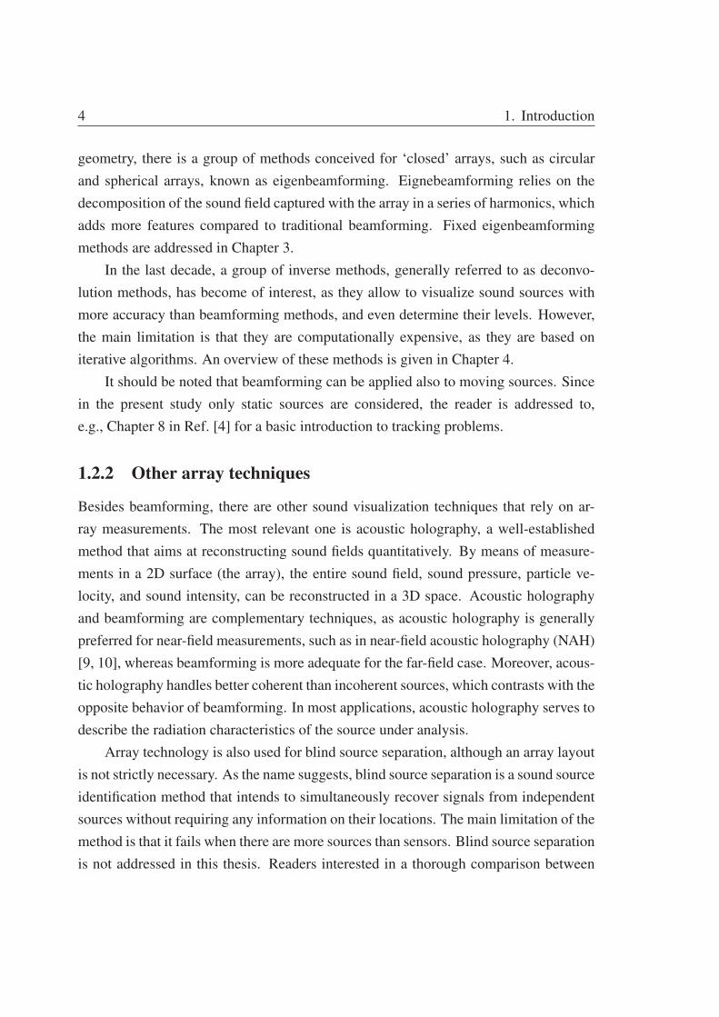
Figure 2.3: Plane wave impinging on an array. The beamformer response presents a main beam when steered
in the direction of the impinging wave, whereas other directions are partially or totally attenuated.
where A is the amplitude, ω represents the angular frequency, related to the frequency
f by ω = 2πf , and ki is the wavenumber vector, with magnitude |ki| = k = ω/c. It
can be shown that the beamformer output, Eq. (2.1), results in
b(t, κ) = Ae−jωtM−1∑m=0
wmej(ki+kκ) · rm . (2.4)
A close inspection of this equation reveals that when the array is steered in the precise
direction κ that satisfies ki = −kκ, the beamformer response presents its maximum
value. When focused toward other directions, the response is partially or totally attenu-
ated. If the array scans all possible directions with the appropriate associated delays, the
resulting beamformed map will present a main lobe around its maximum and sidelobes
elsewhere. This is illustrated in Fig. 2.3.
The weightings wm, often referred to as shading, influence the shape of the main-

14 2. Basic beamforming methods
and sidelobes. They act as spatial windows and their effect is analogous to that observed
with temporal windows in conventional signal processing. In fact, Eq. (2.4) can be
rewritten as
b(t,k) = Ae−jωtW (k− ki), (2.5)
where k = −kκ, and W (k) is the spatial discrete Fourier Transform of the weightings
W (k) =M−1∑m=0
wme−jk · rm . (2.6)
This function is usually known as array pattern. When the weightings follow a uniform
distribution, the array pattern exhibits the narrowest possible main lobe, whereas ta-
pered distributions, such as the triangular and the Hann windows, yield lower sidelobes
at the expense of a wider main lobe [42]. Furthermore, the location of the nulls in the
pattern also depends on the weightings.
In real case scenarios, the pressure captured by the microphones is contaminated
by noise, e.g., background noise and electronic noise. In case of a single plane wave,
the pressure is (cf. Eq. (2.3))
pm(t) = Aej(ki · rm−ωt) + nm(t), (2.7)
where nm(t) is uncorrelated noise present at the mth microphone. Obviously, the pres-
ence of noise influences the response of beamforming systems. However, compared to
a measurement with a single microphone, the combination of many measurements, as
in the case of using a microphone array, leads to a better signal-to-noise ratio (SNR).
Amongst all techniques, it can be shown that delay-and-sum is the most robust against
noise and has, moreover, the ability to suppress uncorrelated noise equally at all fre-
quencies [8].
For broadband signals, it is convenient to implement delay-and-sum beamforming
in the frequency domain. The signal is decomposed in a set of monochromatic plane
waves (i.e., single-frequency waves), each treated independently in the beamforming

2.1 Delay-and-sum beamforming 15
procedure so that the applied phase shifts correspond to the desired delays. That is
b(ω, κ) =
M−1∑m=0
wmpm(ω)ejωτm(κ), (2.8)
where pm(ω) is the discrete Fourier Transform of the signal measured with the mth
sensor. The time domain version can be simply obtained with the inverse discrete
Fourier Transform of b(ω, κ).
A common practice when dealing with stationary sound fields is to formulate delay-
and-sum beamforming in the frequency domain using the averaged cross-spectra of the
input signals. From Eq. (2.8), the power output can be written as
|b(ω,κ)|2 =M−1∑m=0
M−1∑n=0
wmw∗npm(ω)p∗n(ω)e
jω(τm(κ)−τn(κ)), (2.9)
where ( · )∗ denotes complex conjugation. For the sake of simplicity, the weightings are
set to unity in the following. Let us now consider the averaged cross-spectral matrix∗
C =
⎡⎢⎢⎢⎢⎢⎢⎢⎣
c00 c01 c02 · · · c0(M−1)
c11 c11 c12 · · · c1(M−1)
c20 c21 c22 · · · c2(M−1)
......
.... . .
...
c(M−1)0 c(M−1)1 c(M−1)2 · · · c(M−1)(M−1)
⎤⎥⎥⎥⎥⎥⎥⎥⎦, (2.10)
where
cmn(ω) = pm(ω)p∗n(ω), (2.11)
is the averaged cross-spectrum between the signals captured at the mth and nth sensors,
being
cmn(ω) = c∗nm(ω). (2.12)
By using the cross-spectral matrix, the output power of the beamformer can be rewritten
∗Note that the frequency dependence in the matrix is omitted.

16 2. Basic beamforming methods
as
|b(ω, κ)|2 =M−1∑m=0
cmm(ω) +M−1∑m=0
M−1∑n=0n �=m
cmn(ω)ejω(τm(κ)−τn(κ)). (2.13)
As can be seen, the first sum of this expression involves the diagonal elements, i.e., the
auto-spectral terms, cmm(ω), whereas the second sum accounts for off-diagonal terms,
cmn(ω). Note that the diagonal elements contain amplitude information plus self-noise.
However, they do not carry phase information, and therefore, do not help in determining
the source location. That is not the case for the cross-spectra elements; they contain the
relative phase between each pair of sensors, and thus are essential for the beamforming
process. Furthermore, self-noise is not present in these terms, as it is uncorrelated
across channels. Therefore, it seems reasonable to remove the diagonal elements. This
procedure, known as diagonal removal, decreases the level of the sidelobes, resulting
in a clearer beamformed map [43]. However, the price to pay for this operation is that
the resulting levels are biased.
The sound field at the array position can be generically described as the superposition
of waves created by different sources so that waves arrive from different directions.
When waves are incoherent, the beamformer output is equivalent to the superposition
of outputs for each wave [12]. If the sources are sufficiently far from each other, they
can be successfully identified. However, in the presence of coherent waves most beam-
formers fail. This problem, which appears, for instance, when dealing with (coherent)
reflections, is often disregarded in the modern literature [2]. However, some studies
have elaborated on this aspect, e.g., Refs.[44, 45].
Until now only sources in the far field, and thus, plane waves at the array posi-
tion, have been assumed. In this situation only the (angular) direction of the sources
can be identified. Their distance to the array cannot be determined, as, in fact, the
beamformer is focused toward an infinite distance. In contrast, to localize sources
in the near field, a finite focus distance has to be considered, together with spherical
wavefronts. This is illustrated in Fig. 2.4, where the array is steered toward a point
located at r. Geometrical considerations show that, in order to align the signals at the
sensor positions, the delays required for delay-and-sum beamforming are given by
2.1 Delay-and-sum beamforming 17
rm
originarray
r|r− rm|
|r| − |r− rm|
focus point
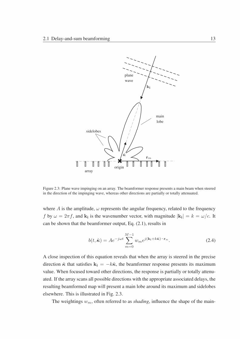
Figure 2.4: Beamformer focused toward a point in the near field. Spherical waves are expected at the array
position.
τm =|r| − |r− rm|
c. (2.14)
Since the amplitude of spherical waves decays with the distance, it is possible to com-
pensate for it by including amplitude corrections in the beamforming algorithm [46].
In what follows, only sources in the far field of the array, and thus, planar wave-
fronts at the array position, are considered.
2.1.1 Uniform linear array
A uniform linear array, the simplest array geometry, serves to illustrate the performance
of a delay-and-sum beamformer. This array consists of a number of sensors placed in a
line with uniform spacing, as shown in Fig. 2.5.
x
z
0 1 M − 1
ϑs
ki
d d
κ
ϑ
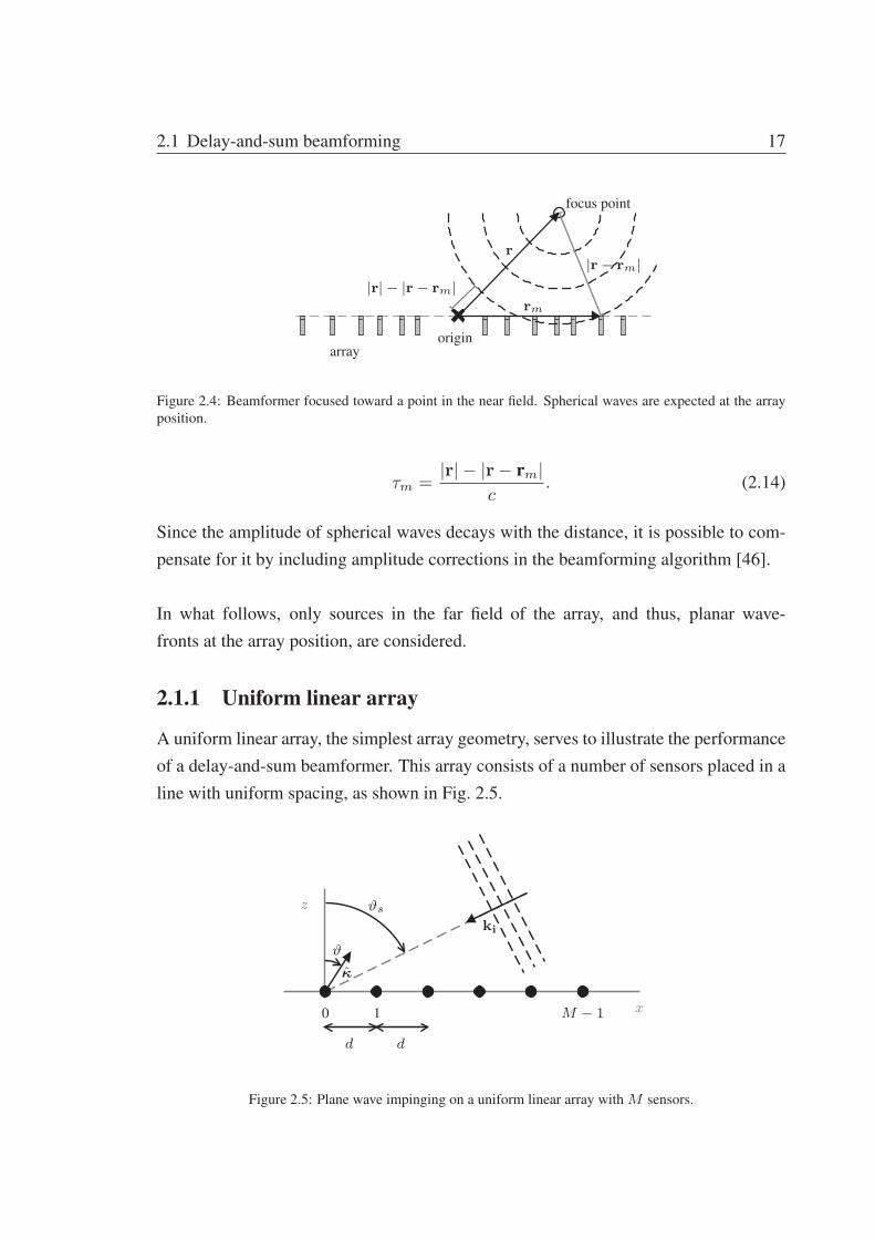
Figure 2.5: Plane wave impinging on a uniform linear array with M sensors.
18 2. Basic beamforming methods
From the geometrical considerations given in Fig. 2.5, the mth array sensor is
located at
rm =
⎡⎢⎣
md
0
0
⎤⎥⎦ , m = 0, . . . ,M − 1, (2.15)
where d is the spacing between sensors. Moreover, when the system is steered toward
the direction given by the polar angle ϑ, here defined from −180◦ to 180◦, the steering
vector κ becomes
κ =
⎡⎢⎣
sinϑ
0
cosϑ
⎤⎥⎦ . (2.16)
Let us assume that the array captures a plane wave with amplitude A and wavenumber
vector
ki = −k
⎡⎢⎣
sinϑs
0
cosϑs
⎤⎥⎦ , (2.17)
where ϑs is the angular position of the source. Expressed in these terms, delay-and-sum
beamforming, Eq. (2.4), becomes
b(t, ϑ) = Ae−jωtM−1∑m=0
wme−jk(sinϑs−sinϑ)md. (2.18)
Notice that this expression does not depend on the azimuth angle ϕ, which implies
that a linear array cannot discriminate between waves arriving from different azimuthal
directions.
Considering a uniform amplitude weighting wm = 1, the output reduces to
b(t, ϑ) = Ae−jωt 1− e−jk(sinϑs−sinϑ)Md
1− e−jk(sinϑs−sinϑ)d. (2.19)
After some rearrangement, the corresponding directivity pattern (or beam pattern) re-
sults in
|b(ϑ)| = |A|∣∣∣∣ sin(π(sinϑs − sinϑ)Md/λ)
sin(π(sinϑs − sinϑ)d/λ)
∣∣∣∣ , (2.20)
where λ is the wavelength, λ = c/f . As an example, the directivity pattern of a uniform
linear array with 10 microphones is shown in Fig. 2.6, when A = 2, d/λ = 0.3 and
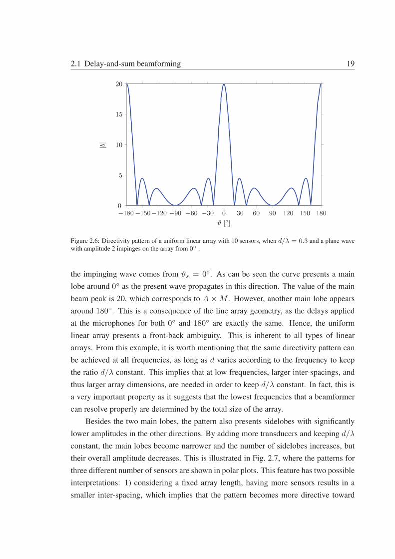
2.1 Delay-and-sum beamforming 19
|b|
ϑ [◦]−180−150−120 −90 −60 −30 0 30 60 90 120 150 1800
5
10
15
20
Figure 2.6: Directivity pattern of a uniform linear array with 10 sensors, when d/λ = 0.3 and a plane wave
with amplitude 2 impinges on the array from 0◦ .
the impinging wave comes from ϑs = 0◦. As can be seen the curve presents a main
lobe around 0◦ as the present wave propagates in this direction. The value of the main
beam peak is 20, which corresponds to A × M . However, another main lobe appears
around 180◦. This is a consequence of the line array geometry, as the delays applied
at the microphones for both 0◦ and 180◦ are exactly the same. Hence, the uniform
linear array presents a front-back ambiguity. This is inherent to all types of linear
arrays. From this example, it is worth mentioning that the same directivity pattern can
be achieved at all frequencies, as long as d varies according to the frequency to keep
the ratio d/λ constant. This implies that at low frequencies, larger inter-spacings, and
thus larger array dimensions, are needed in order to keep d/λ constant. In fact, this is
a very important property as it suggests that the lowest frequencies that a beamformer
can resolve properly are determined by the total size of the array.
Besides the two main lobes, the pattern also presents sidelobes with significantly
lower amplitudes in the other directions. By adding more transducers and keeping d/λ
constant, the main lobes become narrower and the number of sidelobes increases, but
their overall amplitude decreases. This is illustrated in Fig. 2.7, where the patterns for
three different number of sensors are shown in polar plots. This feature has two possible
interpretations: 1) considering a fixed array length, having more sensors results in a
smaller inter-spacing, which implies that the pattern becomes more directive toward

20 2. Basic beamforming methods
0◦30◦
60◦
90◦
120◦
150◦180◦
-150◦
-120◦
-90◦
-60◦
-30◦
-30-20-10 0
(a) M = 5
0◦30◦
60◦
90◦
120◦
150◦180◦
-150◦
-120◦
-90◦
-60◦
-30◦
-30-20-10 0
(b) M = 10
0◦30◦
60◦
90◦
120◦
150◦180◦
-150◦
-120◦
-90◦
-60◦
-30◦
-30-20-10 0
(c) M = 20
Figure 2.7: Influence of the number of transducers on the beamforming pattern of a uniform linear array. The
magnitude is expressed in dB and normalized to A×M . A plane wave approaches the array from 0◦. In all
cases d/λ = 0.3
high frequencies (a smaller wavelength is needed in order to keep d/λ constant.) And
2) assuming a constant space between sensors, increasing the number of sensors is
equivalent to extending the array, which implies that for a given frequency, the larger the
array, the more directive the pattern. This agrees with the previous discussion regarding
array size and low frequencies.
Similarly to the effect of increasing the number of sensors, the pattern becomes
more directive with increasing the ratio d/λ, as can be seen in Fig. 2.8. However,
the case d/λ = 1.2 shows replicas of the main lobe in unexpected directions. These
replicas, usually called grating lobes, are caused by the aliasing effect, which is a con-
sequence of undersampling the space with a finite number of transducers. The aliased
replicas occur when d/λ > 0.5, which corresponds to the Nyquist sampling criterion
in space. In fact, this criterion determines the highest frequency the array can capture
without sampling error. The aliasing effect can be pushed beyond the Nyquist criterion,
and thus, toward higher frequencies, by using irregular arrays. With an irregular layout,
the level of the sidelobes is kept relatively low for a wider frequency range, and aliasing
occurs at those frequencies where the average element spacing is several wavelengths;
up to about 4λ according to Ref. [47], which is significantly above the Nyquist criterion
(λ/2). Ideally, aliasing can only be totally avoided in the hypothetical case of using
an array of sensors placed infinitely close to each other, or alternatively, by means of
scanning the sound field in a continuous manner. Recent studies have shown that this is
possible with a laser beam, as in the acousto-optic beamformer [40].

2.1 Delay-and-sum beamforming 21
0◦30◦
60◦
90◦
120◦
150◦180◦
-150◦
-120◦
-90◦
-60◦
-30◦
-30-20-10 0
(a) d/λ = 0.3
0◦30◦
60◦
90◦
120◦
150◦180◦
-150◦
-120◦
-90◦
-60◦
-30◦
-30-20-10 0
(b) d/λ = 0.5
0◦30◦
60◦
90◦
120◦
150◦180◦
-150◦
-120◦
-90◦
-60◦
-30◦
-30-20-10 0
(c) d/λ = 1.2
Figure 2.8: Influence of the ratio d/λ on the beamforming pattern of a uniform linear array with 10 sensors.
The magnitude is expressed in dB and normalized to A×M . A plane wave approaches the array from 0◦.
0◦30◦
60◦
90◦
120◦
150◦180◦
-150◦
-120◦
-90◦
-60◦
-30◦
-30-20-10 0
(a) ϑs = 0◦
0◦30◦
60◦
90◦
120◦
150◦180◦
-150◦
-120◦
-90◦
-60◦
-30◦
-30-20-10 0
(b) ϑs = 45◦
0◦30◦
60◦
90◦
120◦
150◦180◦
-150◦
-120◦
-90◦
-60◦
-30◦
-30-20-10 0
(c) ϑs = 90◦
Figure 2.9: Influence of the direction of an incident plane wave on the beamforming pattern of a uniform
linear array with 10 sensors. The magnitude is expressed in dB and normalized to A × M . In all cases
d/λ = 0.3
When an incident wave comes from directions other than 0◦ and 180◦, the resulting
main lobe becomes progressively wider toward ±90◦. This can be seen in Fig. 2.9, for
waves arriving from 0◦, 45◦, and 90◦. Due to the front-back ambiguity, a replica of the
main lobe always appears at (180◦ − ϑs) if ϑs ≥ 0, or at (−180◦ − ϑs) if ϑs < 0. A
pattern that depends on the focusing direction is usually referred to as shift-variant.
2.1.2 Uniform circular array
Two of the main weaknesses that uniform linear arrays exhibit, namely the front-back
ambiguity and the pattern dependency on the steering direction, can be solved if uniform

22 2. Basic beamforming methods
x
y
0
1
M − 1
ϕs
ki
R
κ ϕ
(a) Top view
z
x
θ
01
M − 1
κ
kiθs
(b) Side view
Figure 2.10: Plane wave impinging on a uniform circular array with M sensors.
circular arrays are used instead. This array geometry is characterized by having M
sensors uniformly distributed in a circle, as illustrated in Fig. 2.10. The position of the
mth sensor is in this case given by
rm = R
⎡⎢⎣
cos (2πm/M)
sin (2πm/M)
0
⎤⎥⎦ , m = 0, . . . ,M − 1, (2.21)
where R is the radius of the circle. According to geometrical model given in Fig. 2.10,
the array steering vector, and the wavenumber vector of a wave arriving from (θs, ϕs),
are
κ =
⎡⎢⎣
sin θ cosϕ
sin θ sinϕ
cos θ
⎤⎥⎦ , (2.22)
and
ki = −k
⎡⎢⎣
sin θs cosϕs
sin θs sinϕs
cos θs
⎤⎥⎦ . (2.23)
Using the three previous expressions, the delay-and-sum output can be easily obtained
2.1 Delay-and-sum beamforming 23
0◦30◦
60◦
90◦
120◦
150◦180◦
210◦
240◦
270◦
300◦
330◦
-30-20-10 0
(a) ϕs = 0◦
0◦30◦
60◦
90◦
120◦
150◦180◦
210◦
240◦
270◦
300◦
330◦
-30-20-10 0
(b) ϕs = 130◦
0◦30◦
60◦
90◦
120◦
150◦180◦
210◦
240◦
270◦
300◦
330◦
-30-20-10 0
(c) ϕs = 250◦
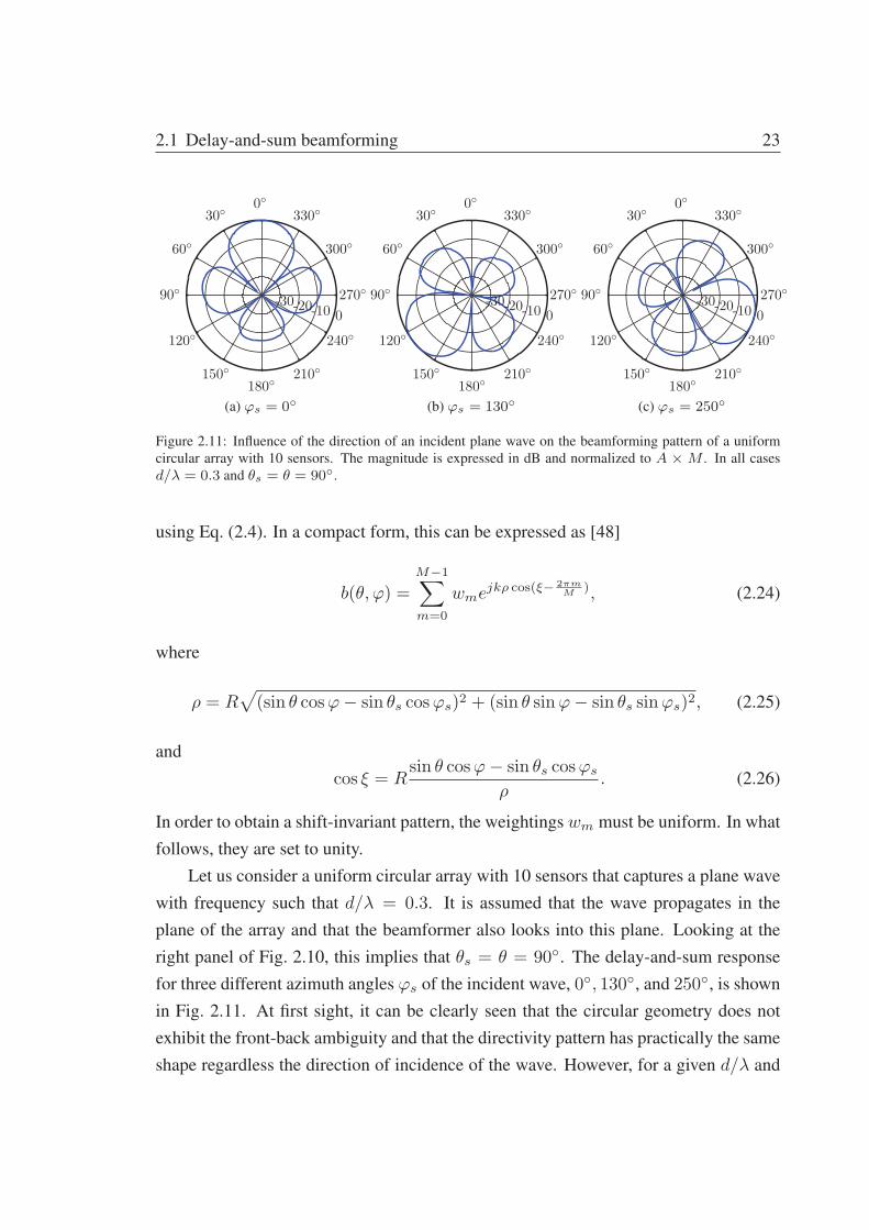
Figure 2.11: Influence of the direction of an incident plane wave on the beamforming pattern of a uniform
circular array with 10 sensors. The magnitude is expressed in dB and normalized to A × M . In all cases
d/λ = 0.3 and θs = θ = 90◦.
using Eq. (2.4). In a compact form, this can be expressed as [48]
b(θ, ϕ) =
M−1∑m=0
wmejkρ cos(ξ− 2πmM ), (2.24)
where
ρ = R√
(sin θ cosϕ− sin θs cosϕs)2 + (sin θ sinϕ− sin θs sinϕs)2, (2.25)
and
cos ξ = Rsin θ cosϕ− sin θs cosϕs
ρ. (2.26)
In order to obtain a shift-invariant pattern, the weightings wm must be uniform. In what
follows, they are set to unity.
Let us consider a uniform circular array with 10 sensors that captures a plane wave
with frequency such that d/λ = 0.3. It is assumed that the wave propagates in the
plane of the array and that the beamformer also looks into this plane. Looking at the
right panel of Fig. 2.10, this implies that θs = θ = 90◦. The delay-and-sum response
for three different azimuth angles ϕs of the incident wave, 0◦, 130◦, and 250◦, is shown
in Fig. 2.11. At first sight, it can be clearly seen that the circular geometry does not
exhibit the front-back ambiguity and that the directivity pattern has practically the same
shape regardless the direction of incidence of the wave. However, for a given d/λ and
24 2. Basic beamforming methods
0◦30◦
60◦
90◦
120◦
150◦180◦
210◦
240◦
270◦
300◦
330◦
-30-20-10 0
(a) d/λ = 0.3
0◦30◦
60◦
90◦
120◦
150◦180◦
210◦
240◦
270◦
300◦
330◦
-30-20-10 0
(b) d/λ = 0.5
0◦30◦
60◦
90◦
120◦
150◦180◦
210◦
240◦
270◦
300◦
330◦
-30-20-10 0
(c) d/λ = 1.2
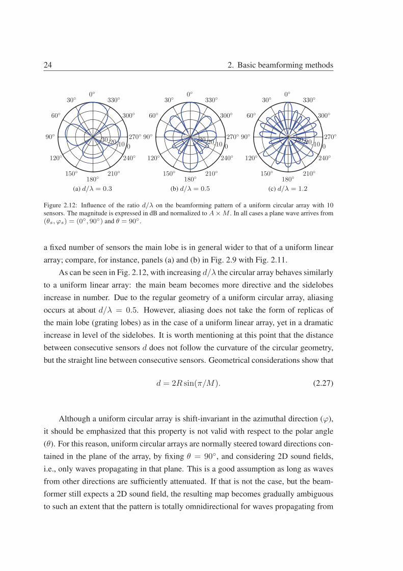
Figure 2.12: Influence of the ratio d/λ on the beamforming pattern of a uniform circular array with 10
sensors. The magnitude is expressed in dB and normalized to A×M . In all cases a plane wave arrives from
(θs, ϕs) = (0◦, 90◦) and θ = 90◦.
a fixed number of sensors the main lobe is in general wider to that of a uniform linear
array; compare, for instance, panels (a) and (b) in Fig. 2.9 with Fig. 2.11.
As can be seen in Fig. 2.12, with increasing d/λ the circular array behaves similarly
to a uniform linear array: the main beam becomes more directive and the sidelobes
increase in number. Due to the regular geometry of a uniform circular array, aliasing
occurs at about d/λ = 0.5. However, aliasing does not take the form of replicas of
the main lobe (grating lobes) as in the case of a uniform linear array, yet in a dramatic
increase in level of the sidelobes. It is worth mentioning at this point that the distance
between consecutive sensors d does not follow the curvature of the circular geometry,
but the straight line between consecutive sensors. Geometrical considerations show that
d = 2R sin(π/M). (2.27)
Although a uniform circular array is shift-invariant in the azimuthal direction (ϕ),
it should be emphasized that this property is not valid with respect to the polar angle
(θ). For this reason, uniform circular arrays are normally steered toward directions con-
tained in the plane of the array, by fixing θ = 90◦, and considering 2D sound fields,
i.e., only waves propagating in that plane. This is a good assumption as long as waves
from other directions are sufficiently attenuated. If that is not the case, but the beam-
former still expects a 2D sound field, the resulting map becomes gradually ambiguous
to such an extent that the pattern is totally omnidirectional for waves propagating from

2.1 Delay-and-sum beamforming 25
0◦30◦
60◦
90◦
120◦
150◦180◦
210◦
240◦
270◦
300◦
330◦
-30-20-10 0
(a) θs = 0◦ and θs = 180◦
0◦30◦
60◦
90◦
120◦
150◦180◦
210◦
240◦
270◦
300◦
330◦
-30-20-10 0
(b) θs = 30◦ and θs = 150◦
0◦30◦
60◦
90◦
120◦
150◦180◦
210◦
240◦
270◦
300◦
330◦
-30-20-10 0
(c) θs = 60◦ and θs = 120◦
0◦30◦
60◦
90◦
120◦
150◦180◦
210◦
240◦
270◦
300◦
330◦
-30-20-10 0
(d) θs = 90◦
Figure 2.13: Influence of the polar angle of an incident plane wave on the beamforming pattern of a uniform
circular array with 10 sensors. The magnitude is expressed in dB and normalized to A × M . In all cases
d/λ = 0.3, ϕs = 0◦ and θ = 90◦.
θs = 0◦ and θs = 180◦. This can be seen in Fig. 2.13. In practice, waves with polar
angles θs up to ±30◦ off-plane are generally detected successfully.
2.1.3 Spherical array
Spherical arrays consist of a number of sensors distributed over the surface of a sphere,
which can be open (or transparent) or not. Unlike circular arrays, which have difficulties
with waves propagating out-of-plane, spherical arrays have the ability to map 3D sound
fields effectively. Furthermore, some layouts can provide a shift-invariant pattern for
the entire 3D space. This will be later addressed in Sec. 3.1.2. The geometrical model
assumed for a spherical array is shown in Fig. 2.14. In this case, the position of the mth
microphone is given by

26 2. Basic beamforming methods
z
y
θ
κ
ki
θs
x
ϕ
ϕs
Figure 2.14: Plane wave impinging on a spherical array with M sensors.
rm = R
⎡⎢⎣
sin θm cosϕm
sin θm sinϕm
cos θm
⎤⎥⎦ , m = 0, . . . ,M − 1, (2.28)
where R is the radius of the sphere, and θm and ϕm are the polar and the azimuth angles
of the mth transducer. The focus direction κ and the wavenumer vector of an incident
plane wave are given by Eqs. (2.22) and (2.23), respectively.
2.2 Performance indicators
It is apparent from the previous section that several aspects, for instance, geometry,
number of transducers, and spacing, influence the beamformer response. It is therefore
necessary to make use of performance indicators to assess and compare beamforming
systems. Most measures of performance found in the literature are often adapted from
other fields, such as electromagnetism (antenna theory) and optics. A brief description
of the most relevant ones is given in the following.
2.2 Performance indicators 27
Measures of beam pattern
Resolution: Defined as the −3 dB width of the main lobe of the directivity pattern
and measured in degrees or radians. It is also known as the 3 dB beamwidth,
the half-power beamwidth, and the angular resolution. This measure, which is
adapted from antenna theory (see, e.g., Ref. [49]) gives the minimum angle at
which two incoherent sources can be resolved. Moreover, it is an indicator of
directivity. The lower the value, the more directive the beamformer is.
Maximum sidelobe level (MSL): Given by the difference in level in dB between
the peak of the highest sidelobe in the beam pattern to the peak of the main
lobe [12]. This measure is also adapted from antenna theory and in the antenna
community it is commonly referred to as SLL (sidelobe level) [50]. The MSL
is complementary to the resolution, as it is not about directivity, yet a descriptor
of how sensitive the beamformer is toward unwanted directions. Obviously, the
larger the level difference between main- and maximum sidelobe, the better. It
can be shown that this measure is more sensitive to noise than the resolution.
Peak-to-zero distance or Rayleigh resolution limit: Given by the angular difference
between the position of the peak of the main lobe of the beam pattern and the
position of its closest null. It determines the ability of the array to resolve two
incoherent plane waves based on the Rayleigh criterion [51], adapted from optics
theory. This criterion states that two plane waves are resolved when the main
peak of the beam pattern of one falls on the null closest to the main peak of the
beam pattern of the other one. This measure is an alternative to the resolution
based on the −3 dB width, as half the beamwidth between the nulls of the main
lobe is approximately equal to the −3 dB beamwidth [52].
Figure 2.15 illustrates how the resolution, the MSL, and the peak-to-zero distance
can be extracted from a given beam pattern.
Other measures
Directivity index (DI): Defined as the ratio of the beamformer response in the looking
direction to the average response over all directions. Expressed on logarithmic

28 2. Basic beamforming methods
RESMSL
−3 dB
PTZ
ϕ [◦]
Mag
nitu
deof
b[d
B]
0 30 60 90 120 150 180 210 240 270 300 330 360−35
−30
−25
−20
−15
−10
−5
0
5
Figure 2.15: Calculation of the resolution (RES), the MSL, and the peak-to-zero (PTZ) distance from a given
beam pattern.
scale [52, 53], the DI can be written as
DI = 10 log
(|b(θs, ϕs)|2
14π
∫ 2π
0
∫ π
0|b(θ, ϕ)|2 sin θ dθ dϕ
). (2.29)
This measure can be regarded as the array gain against isotropic noise (noise
distributed uniformly over a sphere) [42]. The higher the DI, the better.
Array gain: Reflects the improvement in SNR achieved by using an array. It is defined
as the ratio of the SNR at the array output to the SNR at a single sensor subject to
different types of noise [4]. Usually isotropic acoustical noise is considered [8].
White noise gain (WNG): Measured as the array gain, but considering that the SNR
at every sensor is due to spatially uncorrelated white noise [8]. It can also be
regarded as the ratio of the signal power at the output of the beamformer to the
sensor self-noise power assuming a unity variance noise [54]. The WNG is an
indicator of the robustness of the array against deviations in the practical imple-
mentation, such as sensor self-noise, positioning errors, and amplitude and phase
variations. The higher the WNG, the more robust the array is. It can be shown
that the optimal WNG equals the number of microphones, for frequencies below

2.2 Performance indicators 29
the Nyquist frequency, and is achieved with delay-and-sum beamforming with a
uniform weighting [42].
Usually, the resolution and the MSL are examined together as they provide direct
values related to the beam pattern that complement each other to give an idea of its
shape. These two indicators can be seen in Fig. 2.16 as a function of frequency for a
delay-and-sum beamformer based on a uniform circular array with 12 sensors and 11.9
cm of radius.†. A uniform weighting, a focusing direction of 180◦, and ideal (noise
free) conditions are assumed. As can be seen, the resolution improves with increasing
frequency, which means that the main beam becomes narrower. On the other hand,
the MSL indicates that at low frequencies the sidelobes are non-existent, but they arise
with increasing frequency. Inspection of these two performance indicators together
suggest that the beamformer response is omnidirectional at the lowest frequencies, but
with increasing frequency the directivity increases, although this is accompanied by an
increase in level of sidelobes, which stagnates at a certain frequency.
The DI of the array previously examined is showed in Fig. 2.17, together with the
WNG. In this case, the DI at the lowest frequencies is 0 dB, which means that the beam
pattern is omnidirectional. With increasing frequency, the DI increases progressively,
indicating, thus, that the array becomes more and more directive. In contrast to the
resolution, the DI provides a value related to the array directivity that considers not
only the width of the main lobe, but also the sidelobes. This makes it impossible to
predict a beam pattern via the DI, as becomes apparent from the inspection of Fig. 2.17.
On the other hand, the WNG is constant across frequency, being equal to 10.8 dB,
i.e., 12 in a linear scale, corresponding to the number of array microphones, as expected
from the fact that delay-and-sum with uniform weighting provides the optimal WNG.
It should be noted that while the resolution, the MSL, and the DI can be extracted from
experimental results, this is not possible with the WNG, as this is a theoretical measure.
In the microphone array community, the DI and the WNG are typically preferred
for the numerical analysis of array designs, see, e.g., Refs. [8, 19, 54, 55]. The res-
olution and the MSL are less used, but nevertheless they have proven to be a useful
evaluation tool, e.g., in Refs. [12, 56–58]. While the resolution can be related to the
DI, as both are measures of directivity, the MSL can be used to examine the robustness
†An array with these characteristics is used in Paper A. Its Nyquist frequency is about 2.7 kHz.

30 2. Basic beamforming methods
Frequency [Hz]
Res
olut
ion
[◦]
0 500 1000 1500 2000 25000
60
120
180
240
300
360
(a) Resolution
Frequency [Hz]
MSL
[dB
]
0 500 1000 1500 2000 2500−70
−60
−50
−40
−30
−20
−10
0
(b) MSL
Figure 2.16: Resolution and MSL obtained with a delay-and-sum beamformer based on a uniform circular
array with 12 sensors and 11.9 cm of radius. The array is focused toward 180◦.

2.2 Performance indicators 31
Frequency [Hz]
DI[
dB]
0 500 1000 1500 2000 2500−2
0
2
4
6
8
10
(a) DI
Frequency [Hz]
WN
G[d
B]
0 500 1000 1500 2000 25000
2
4
6
8
10
12
14
(b) WNG
Figure 2.17: DI and WNG obtained with a delay-and-sum beamformer based on a uniform circular array with
12 sensors and 11.9 cm of radius. The array is focused toward 180◦.

32 2. Basic beamforming methods
of the system, although this is not a direct measure as the WNG is. Since the noise
captured by the system affects basically the level of the sidelobes of the beamforming
response, this makes the resulting MSL deviate from the MSL that would be obtained
in the absence of noise. The higher the deviation, the less robust the system is.
In the contributing papers of this thesis, the performance of the suggested methods
is examined basically by means of the resolution and the MSL for the following main
reasons:
1. For sound source localization purposes the spatial sensitivity of the array is a very
important factor. In this sense, the resolution is a very appropriate parameter.
In combination with the MSL, these measures provide a better picture of the
behavior of the beam pattern than DI and WNG.
2. Both resolution and MSL can be extracted from experimental data and not only
from numerical data as in the case of the WNG‡, which is crucial for the valida-
tion of the methods suggested in the papers.
3. For the reader not familiar with microphone arrays, the resolution and the MSL
are simpler to interpret than the DI and the WNG.
‡Note that although the DI can also be extracted from experimental measurements, this is rarely seen in
the literature.

Chapter 3
Eigenbeamforming
3.1 Introduction
Eigenbeamforming, also known as eigenbeam beamforming, is a rather new category
of methods that rely on ‘closed’ geometries, such as a sphere or a circle. The sound
field captured by arrays that fulfill this condition can be decomposed into a sum of
orthogonal terms that satisfy the wave equation in the coordinate system that best suits
the array geometry. Combination of these orthogonal terms, known as harmonics or
phase modes, makes it possible to form a detection beam. An eigenbeamforming system
consists of two stages, see Fig. 3.1; in the first stage, the pressure measured with the
array is decomposed in a set of harmonics, and in the second stage, usually referred
to as modal beamformer, the coefficients of the harmonics are weighted and added
together to provide the final beamforming output [32]. The fundamental difference
from traditional beamforming lays on the fact that the latter is based on applying the
signal processing algorithms directly to the signals captured by the microphones. It
should be noted that the concept of using phase modes had been already explored in the
past in the field of electromagnetism, for antenna design; see, e.g., Refs. [59–68].
Although in principle many array shapes are possible for eigenbeamforming, only
those that have a well-defined geometry in the conventional coordinate systems are used
in practice. The most popular geometry is the spherical one [69–75], followed by the
circular [19, 55, 76–79] and the spheroidal [80].
33

34 3. Eigenbeamforming
0
1
2
M − 1pM−1
p1
p2b
p0
C−1
CN
Sound
field
decomposition
Modal
beamformer
C0
C−N
C1
Figure 3.1: Eigenbeamforming procedure. The sound field captured by the array sensors is decomposed in
a series of orthogonal functions, whose coefficients are weighted in the modal beamformer stage to yield the
final output b.
3.1.1 Eigenbeamforming for circular arrays
The concepts behind eigenbeamforming are here briefly described assuming an open
uniform circular array, as the one shown in Fig. 2.10 on page 22. Given the circular
symmetry, the sound field can be decomposed in a Fourier series in the azimuth coor-
dinate, ϕ, so that, at the array radius, the sound pressure can be written in the spatial
frequency domain as [10]
p(kR, ϕ) =
∞∑n=−∞
Cn(kR)ejnϕ, (3.1)
where the terms ejnϕ, often referred to as circular harmonics, form a set of orthogonal
functions,1
2π
∫ 2π
0
ejnϕ(ejνϕ)∗dϕ = δnν , (3.2)
where δnν is the Kronecker delta function, which equals unity when n = ν and zero
otherwise, and Cn(kR) is the nth order Fourier coefficient,
Cn(kR) =1
2π
∫ 2π
0
p(kR, ϕ)e−jnϕdϕ. (3.3)

3.1 Introduction 35
If a plane wave with amplitude A, created at ϕs, is present in the sound field, it can be
shown that the coefficients become [81]
Cn(kR) = AQn(kR)e−jnϕs , (3.4)
where Qn(kR) is a function that depends on the boundary conditions of the uniform
circular array, that is, for example, whether the array is mounted on a baffle or not, as
will be seen later. In the case of a uniform circular array suspended in free-space,
Qn(kR) = (−j)nJn(kR), (3.5)
where Jn(kR) is a Bessel function of the first kind and order n.
In theory, the sound pressure is represented by infinitely many Fourier coefficients.
In practice, it can be shown that the contribution of those orders higher in magnitude
than kR is very small [42]. Therefore, the representation of the sound field is often
limited, or truncated, to a maximum order N that satisfies
N ≈ kR. (3.6)
It is worth noting that less orders are required for representing the low frequencies
compared to the high frequencies.
With an array of transducers, the sound pressure is sampled at discrete positions,
rather than in a continuous circle. This implies that the coefficients defined in Eq. (3.3)
need to be approximated by
Cn(kR) ≈M−1∑m=0
αmp(kR, ϕm)e−jnϕm , (3.7)
where the term αm is an integration factor that ensures the discrete orthogonality prop-
erty of the circular harmonics
M−1∑m=0
αmejnϕm(ejνϕm
)∗ ≈ δnν . (3.8)
Given the constant sensor spacing of a uniform circular array, αm = 1/M . An ad-
ditional consequence of the sampling theorem in space is that the number of array

36 3. Eigenbeamforming
sensors required to capture the sound field up to order N must be larger than 2N
(M > 2N) [42]. The error due to sampling a continuous circle with a limited number
of sensors and the error for considering a finite number of harmonics for representing
the sound field are analyzed thoroughly in Refs. [18, 81].
The output of an eigenbeamforming system based on a circular array results from
weighting and combining the Fourier coefficients obtained with the decomposition of
the sound field, that is,
b(kR) =N∑
n=−N
wn(kR)Cn(kR), (3.9)
where wn(kR) is the weighting associated to the nth order Fourier coefficient Cn(kR).
Analogous to the influence on the weighting observed in Chapter 2 for delay-and-sum
beamforming, the output of the eigenbeamformer strongly depends on the these param-
eters. When the weightings take the form
wn(kR) =1
Qn(kR)ejnϕl , (3.10)
where ϕl is the looking direction of the array, the beamforming technique is referred
to as circular harmonics beamforming. This method, described and examined in Pa-
pers A and B, provides a response rotationally symmetric around the azimuthal looking
direction, i.e., the resulting pattern is shift-invariant. When using these weightings it
is particularly important to limit the orders in the beamforming algorithm to a value
N close to that given in Eq. (3.6) to avoid amplification of noise. Usually, the maxi-
mum number of orders is chosen as N = �kR�, where � · � is the ceiling function [81].
If higher orders are considered, the value Qn(kR) in the denominator tends to zero,
boosting, in this way, noise captured in the measurements. Therefore, the truncation
of orders can be regarded as a regularization method. The main characteristic of this
technique is that the output depends on the number of harmonics taken into account in
the algorithm; see Appendix A for further details.
Interestingly, delay-and-sum beamforming can also be characterized in terms of
eigenbeamforming, making use of the weightings
wn(kR) = Q∗n(kR)ejnϕl . (3.11)
3.1 Introduction 37
These weightings also ensure a shift-invariant pattern [16].
Besides circular harmonics beamforming and delay-and-sum beamforming, other
methods based on eigenbeam processing with a uniform circular array of microphones
can be found in the literature. For instance, Ref. [18] adapts various adaptive methods,
such as MUSIC and ESPRIT∗, to the circular geometry.
Eigenbeamforming makes it easier to deal with baffled arrays, arrays whose ele-
ments are flushed-mounted on the surface of an object or a scatterer. By simply modify-
ing the function Qn(kR) of Eq. (3.4) according to the baffle type, the scattering effect
can be taken into account in the beamforming algorithm. Common baffles suitable
for uniform circular arrays are rigid spheres [19, 55] and cylinders [76]. Less popu-
lar are rigid baffles with a spheroidal shape [79], which can be oblate or prolate, and
baffles with a certain surface impedance [55]. While the scattering effects of spheres,
spheroids, and infinitely-long cylinders, have an exact analytical solution, and so does
the corresponding Fourier coefficients, that is not the case with the scattering from a
finite cylinder.
Arrays with rigid baffles are usually preferred over open arrays for the following
two reasons; firstly, the boundary conditions of a baffle are well defined compared to
open arrays, which in practice are far from being transparent (their structure, preampli-
fiers, cables, etc., obviously alter the sound field [82]). Secondly, baffled arrays provide
a better response than open arrays; in particular, this is noticeable with delay-and-sum
beamforming toward low frequencies, as due to the presence of the baffle, waves need
to travel longer distances before reaching the microphones, which results in an effec-
tive larger array aperture [78]. Of all common types of rigid baffles for circular arrays,
delay-and-sum beamforming performs best with cylinders. The behavior with oblate
and prolate spheroidal baffles lies between those of an open array and a sphere, and a
sphere and an infinite cylinder, respectively [79]. With circular harmonics beamform-
ing, the performance with scatterers is very similar to that with open arrays. The only
difference is that with open arrays the output presents singularities at those frequen-
cies that coincide with the zero-crossings of the Bessel functions in the denominator
of the algorithm; see Eqs. (3.5) and (3.10). With this technique, there is no significant
difference between different types of baffles.
∗ESPRIT stands for ‘estimation of signal parameters via rotational invariance techniques’.

38 3. Eigenbeamforming
3.1.2 Eigenbeamforming for spherical arrays
Spherical arrays are suitable for decomposing a 3D sound field into a series of orthog-
onal terms of the form [10]
Y mn (θ, ϕ) =
√2n+ 1
4π
(n−m)!
(n+m)!Pmn (cos θ)ejmϕ, (3.12)
where Pnm(cos θ) is the associated Legendre function of order m and degree n. These
terms are commonly referred to as spherical harmonics. In the case of a spherical array
of radius R, the pressure at the sphere is given by the Helmholtz equation in spherical
coordinates [16],
p(kR, θ, ϕ) =
∞∑n=0
n∑m=−n
Cmn(kR)Y mn (θ, ϕ), (3.13)
where the terms Cmn(kR) follow
Cmn(kR) =
∫ 2π
0
∫ π
0
p(kR, θ, ϕ)Y mn (θ, ϕ)∗ sin θdθdϕ. (3.14)
Since with an array the pressure is captured at the sensor positions, the coefficients that
result from the decomposition of the sound field are in practice approximated by
Cmn(kR) =
M−1∑i=0
αip(kR, θi, ϕi)Ymn (θi, ϕi)
∗, (3.15)
where θi and ϕi are angular coordinates of the ith microphone and αi is an integration
factor associated to the ith microphone. This parameter enforces the orthogonality
of the spherical harmonics up to order N , such that the resulting coefficients are free
of error up to that order [20]. By analogy to the case of eigenbeamforming with a
circular sphere, it can be shown that the coefficients Cmn(kR) can be weighted before
adding them together to form a beam in a particular direction. Eigenbeamforming with
spherical arrays is well documented in the literature. The reader interested in this topic
is addressed to, e.g., Ref. [16, 54].
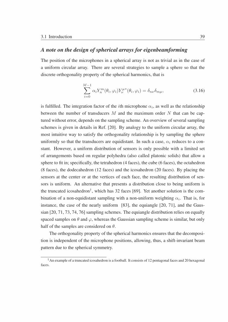
3.1 Introduction 39
A note on the design of spherical arrays for eigenbeamforming
The position of the microphones in a spherical array is not as trivial as in the case of
a uniform circular array. There are several strategies to sample a sphere so that the
discrete orthogonality property of the spherical harmonics, that is
M−1∑i=0
αiYmn (θi, ϕi)Y
μν
∗(θi, ϕi) = δnνδmμ, (3.16)
is fulfilled. The integration factor of the ith microphone αi, as well as the relationship
between the number of transducers M and the maximum order N that can be cap-
tured without error, depends on the sampling scheme. An overview of several sampling
schemes is given in details in Ref. [20]. By analogy to the uniform circular array, the
most intuitive way to satisfy the orthogonality relationship is by sampling the sphere
uniformly so that the transducers are equidistant. In such a case, αi reduces to a con-
stant. However, a uniform distribution of sensors is only possible with a limited set
of arrangements based on regular polyhedra (also called platonic solids) that allow a
sphere to fit in; specifically, the tetrahedron (4 faces), the cube (6 faces), the octahedron
(8 faces), the dodecahedron (12 faces) and the icosahedron (20 faces). By placing the
sensors at the center or at the vertices of each face, the resulting distribution of sen-
sors is uniform. An alternative that presents a distribution close to being uniform is
the truncated icosahedron†, which has 32 faces [69]. Yet another solution is the com-
bination of a non-equidistant sampling with a non-uniform weighting αi. That is, for
instance, the case of the nearly uniform [83], the equiangle [20, 71], and the Gaus-
sian [20, 71, 73, 74, 76] sampling schemes. The equiangle distribution relies on equally
spaced samples on θ and ϕ, whereas the Gaussian sampling scheme is similar, but only
half of the samples are considered on θ.
The orthogonality property of the spherical harmonics ensures that the decomposi-
tion is independent of the microphone positions, allowing, thus, a shift-invariant beam
pattern due to the spherical symmetry.
†An example of a truncated icosahedron is a football. It consists of 12 pentagonal faces and 20 hexagonal
faces.

40 3. Eigenbeamforming
3.2 Papers A and B
3.2.1 Synopsis
Paper A suggests an eigenbeamforming technique for a uniform circular array, called
circular harmonics beamforming. The technique, conceived for mapping sources dis-
tributed from 0 to 360◦, is particularly suitable for environmental noise problems. Cir-
cular harmonics beamforming is compared numerically to delay-and-sum beamform-
ing for both an open array and an array mounted on an infinitely-long rigid cylinder, by
means of the resolution and the MSL. The method is also validated experimentally with
an open array.
Paper B extends the investigation carried out in Paper A to the case of a uniform
circular array mounted on the equator of a rigid sphere, and validates it numerically and
experimentally.
3.2.2 Related work
In 2001, Meyer presented in Ref. [19] a method for beam pattern synthesis based on
the decomposition of the sound field into a series of (circular) harmonics that relied
on a uniform circular array mounted on a rigid sphere. Although the concept was ini-
tially developed for uniform circular arrays, it triggered a series of research projects
involving spherical arrays of microphones, pioneered by Meyer and Elko, Ref. [69],
and Abhayapala and Ward, Ref. [70], in 2002. Their investigations set the foundations
of eigenbeamforming for spherical arrays. In the following years, Rafaely published
several articles on the matter, e.g., Refs. [16, 20, 71, 75]. In particular, the principles of
eigenbeamforming (in that case referred to as phase-mode processing) were described
in Ref. [72], following the approach used in Sec. 3 for the circular geometry, also under
the plane wave assumption. In particular, Rafaely analyzed the response of an eigen-
beamformer whose weightings provided the so-called regular beam pattern, the most
directive pattern (for fixed beamforming) [16], and compared it to delay-and-sum ex-
pressed in eigenbeamforming terms. The results of that study showed that the directiv-
ity achieved with the regular beam pattern exceeds that of delay-and-sum beamforming,
specially at low frequencies, at the expense of robustness to noise. That work was later
supplemented in Ref. [75] with an overview of various eigenbeamforming methods.
Oddly enough, contemporary to Rafaely’s research, Pedersen in Ref. [84] and Song

3.2 Papers A and B 41
in Ref. [85], following an approach different from Rafaely’s, arrived to the expres-
sion for eigenbeamforming with a regular beam pattern, considering, though, spherical
waves. They called the method spherical harmonics beamforming. A year after Song’s
work was published, Haddad and Hald, in Ref. [86], added a scale factor into spherical
harmonics beamforming so that in case of having a rigid sphere, the pressure contribu-
tion would be determined correctly, i.e., without the influence of the scattering effect.
This version of spherical harmonics beamforming was referred to as spherical harmon-
ics angularly resolved pressure (SHARP). This method has been recently extended in
Ref. [57] to provide a smoother response, by means of adding regularization filters.
Similarly to Rafaely’s article on decomposition of sound fields with spherical ar-
rays, Ref. [71], Teutsch and Kellerman in Ref. [76]‡ presented a theoretical analysis of
plane wave decomposition with circular arrays, unbaffled, mounted on a rigid infinitely-
long cylindrical baffle, and mounted on a rigid cylinder of finite-length. In addition,
they derived eigenbeamforming based on the circular geometry, assuming a continuous
aperture instead of the sampled version, i.e., a microphone array. Also, they expressed
two adaptive beamforming algorithms ESPRIT and DETECT, in terms of eigenbeam-
forming and evaluated them with an array mounted on a rigid cylinder, numerically and
experimentally.
3.2.3 Discussion
Inspired by the literature on eigenbeamforming with spherical arrays, Paper A adapts
the theory behind spherical harmonics beamforming to the 2D case with a circular array,
assuming, in this case, plane waves impinging on the array. The proposed beamforming
technique, referred to as circular harmonics beamforming, was originally conceived
in Paper A for localization of environmental noise sources, but it can obviously be
applied to other scenarios where sound sources are distributed over the array azimuth.
It should be noted that 1) the approach followed in Paper A to derive circular harmonics
beamforming is different from the synthesized derivation given in Sec. 3.1.1; and 2) the
article does not include the insight into the technique concerning the influence on the
number of orders given in Appendix A.
While delay-and-sum is omnidirectional at low frequencies, circular harmonics
beamforming presents a certain directivity, namely a resolution of about 112◦ in the
‡This work is also presented in the PhD Thesis by Teutsch, Ref. [18].

42 3. Eigenbeamforming
worst case. Indeed, the response of circular harmonics beamforming in terms of di-
rectivity is better at the lower frequency range than that of delay-and-sum. At high
frequencies, both methods perform similarly. The main drawback of circular harmon-
ics beamforming in comparison with delay-and-sum is its vulnerability to noise, which
essentially affects the sidelobe levels. Circular harmonics beamforming implemented
with an open uniform circular array presents singularities at a few (single) frequencies,
which can be resolved when the array is mounted on a rigid infinitely-long cylinder. In
general terms, though, the overall output pattern with the two array configurations is the
same. By contrast, the pattern of delay-and-sum with the cylindrical scatterer improves
toward low frequencies, as the scatterer makes the array appear larger. Interestingly,
with this configuration both the resolution and the MSL at high frequencies is similar
for both beamforming techniques. However, at low frequencies, the performance with
circular harmonics beamforming still exceeds that of delay-and-sum.
The results of the investigation carried out in Paper A showed that the performance
with a rigid infinitely-long cylindrical scatterer was better over that of an open array,
especially for delay-and-sum beamforming. Since infinitely-long cylinders are not fea-
sible, they are in practice approximated by finite length cylinders. With regard to that,
Teutsch and Kellerman showed in Ref. [76] that a finite cylinder whose length is 1.4
times its radius is enough to approximate an infinitely long cylinder, as its modal re-
sponse becomes fairly similar. This result was later ratified by Granados in Ref. [87].
As an alternative to cylindrical scatterers of finite-length, Paper B suggests to flush-
mount the array on the equator of a rigid sphere, and repeat the comparison carried out
in Paper A. The main advantage of this configuration is that the scattering produced by
this geometry has an exact analytical solution, in contrast to the finite-length cylinder.
With a spherical baffle, circular harmonics beamforming performs in the same manner
as in the infinitely-long cylinder case. However, for delay-and-sum the improvement
is not as good as with the cylinder, because the effective aperture achieved with the
spherical scatterer is smaller.
The novelty of circular harmonics beamforming cannot be entirely attributed to
the author of this thesis as Zhang et al. in Ref. [88] also derived the same technique
under another name and compared it to delay-and-sum for a circular array mounted on
a rigid sphere. Their work, thus, resembles the study presented in Paper B, although
they assessed the beamforming techniques using DI and WNG, and the analysis was
restricted to numerical simulations. In any case, their findings agree in general terms

3.2 Papers A and B 43
with those of Paper B. It should be emphasized that Ref. [88] is not cited in Papers A
and B as the author of this thesis was not aware of the existence of this work at the time
of writing the papers.
The results in Paper B concerning delay-and-sum also agree with those shown by
Daigle et al., in Ref. [55], where the performance of delay-and-sum was analyzed for
circular arrays mounted on spherical baffles using the DI.

44 3. Eigenbeamforming

Chapter 4
Deconvolution methods
4.1 Introduction
Beamforming systems cause unavoidable effects, namely the frequency dependence of
the array resolution and the appearance of sidelobes, which result in beamformed maps
that appear blurred and often difficult to interpret, particularly when several acoustic
sources need to be detected simultaneously. Deconvolution methods intend to deblur
them by removing the artifacts introduced by the array system itself and thereby restor-
ing the original data. These methods rely on the fact that the beamformer output is
a linear combination of the spatial distribution of acoustic sources and the so-called
point-spread function, defined as the beamformer’s response to a point source∗. Math-
ematically, the deconvolution problem can be formulated in the frequency domain as
follows
|b(r)|2 =∑r′∈G
s(r′) ·H(r|r′), (4.1)
where s(r′) is the source power distribution at a position r′ that belongs to the grid of
points G, and H(r|r′) is the point-spread function at r due to a source at r′. It should
be emphasized that the source power distribution is non-negative. In matrix notation,
the previous expression can be written as
b = Hs, (4.2)
∗The point-spread function and the beamformed map are sometimes referred to as the ‘dirty beam’ and
the ‘dirty map’, respectively.
45

46 4. Deconvolution methods
0.5 0 0.5
x [m]0.5 0 0.5
x [m]
0.5
0
0.5
y[m
]
0.5
0
0.5
y[m
]
20
18
16
14
12
10
8
6
4
2
0 dB
Figure 4.1: Beamformed map (left) and clean map after deconvolution (right). Measurement of two uncorre-
lated sources located at 2.7 m from the array. The stars in the beamformed map indicate the position of the
sources. The level of the right source is 10 dB higher. With beamforming the left source is masked, whereas
it becomes visible after deconvolution. Adapted from Ref. [90].
where b is a vector with the power response of the beamformer, H is a matrix that
in each column contains the point-spread functions of each grid point, and s is the
unknown source power distribution vector. The deconvolution methods try, thus, to
compensate for the ‘blurring’ effect of the point-spread function to recover the original
source distribution. Notice that this a discrete inverse problem, and must be treated
carefully to avoid an abrupt amplification of noise, which can often lead to a meaning-
less solution [89]. Deconvolution methods approach this problem by means of iterative
algorithms. The resulting plot of the estimated source distribution is a ‘clean’ version
of the beamformed map: the resolution is improved, and the sidelobes are reduced, or
even suppressed. This is illustrated in Fig. 4.1.
Deconvolution methods are relevant in many fields that involve image restoration.
This problem was first approached for seismology purposes by Robinson [91, 92] back
in 1954, inspired by the previous work done by Wiener in that field [93]. Since then,
deconvolution has been applied to many other research areas, such as radio astron-
omy [94], optical microscopy [95] and image processing [96]. It was not until the
late nineties, that the aeroacoustic community adapted some of the existing decon-
volution methods to deal with sound field visualization problems. That is the case
of CLEAN [97] and Richardson-Lucy [98, 99], both originally developed for astron-
omy and modified for acoustical purposes in Refs. [13] and [100], respectively. While
CLEAN acts directly on the beamformed map, i.e., on the image itself, Richardson-

4.1 Introduction 47
Lucy solves the inverse problem posed in Eq. (4.2) using Bayes’ theorem on condi-
tional probabilities. Other algorithms, adapted from classical non-negative least squares
(NNLS) procedures [101], seek to solve the following optimization problem
minimize 12 ‖Hs− b‖22 , (4.3)
subject to q ≥ 0. (4.4)
That is the case of gradient projection methods, such as the fast Fourier transform-non-
negative least squares method (FFT-NNLS) [100], the gradient projection method with
Barzilai & Borwein steps [102], and the fast iterative shrinkage-thresholding algorithm
(FISTA) [103], examined in Ref. [104] for sound source localization purposes.
Alternatively, there are methods specifically conceived for acoustic purposes. A
number of methods are devoted to static incoherent sound fields. The first method devel-
oped, called the deconvolution approach for the mapping of acoustic sources (DAMAS)
[105, 106], had the main disadvantage that was computationally very heavy. Seeking
for efficiency, other algorithms, such as DAMAS2 [107], SC-DAMAS [108], CLEAN-
SC [109], the covariance matrix fitting (CMF) [108], and the iterative sidelobe cleaner
(ISCA) [110], were implemented based on some assumptions. For example, DAMAS2
relies on a shift-invariant point-spread function, whereas SC-DAMAS, CLEAN-SC and
CMF assume source sparsity. Moreover, DAMAS, DAMAS2, CLEAN, and CLEAN-
SC have been extended in Ref. [111] to deal with moving sources. There are far less
methods capable to deal with coherent sound fields. Examples are DAMAS-C [112],
CMF-C [108], the mapping of acoustic sources (MACS) [113], and the wavespace-
based coherent deconvolution [114]. In this case, CMF-C and MACS rely on spar-
sity, whereas the wavespace coherent deconvolution algorithm assumes a shift-invariant
point-spread function.
The main drawback of deconvolution procedures is that they are in general com-
putationally challenging. It is therefore necessary to find a compromise between the
degree of accuracy, given by the size of the grid and the number of iterations, and
the computational run time. Certain techniques, such as DAMAS2, FFT-NNLS, and
Richardson-Lucy, rely on a shift-invariant beamformer’s point-spread function in order
to use spectral procedures (Fourier-based) to reduce the complexity of the calculations,
and thus, improve efficiency. Since a shift-invariant point-spread function only depends

48 4. Deconvolution methods
on the distance between the source position and the observer position,
H(r|r′) = H(r− r′), (4.5)
the beamformer output, Eq. (4.1), results in a convolution
|b(r)|2 = s(r′) ∗H(r− r′). (4.6)
This relationship makes it possible to tackle the problem in the frequency domain, by
means of expressing the convolution as a multiplication, and, thereby, speed up the
process,
|b(r)|2 = F−1 [F [s(r′)]F [H(r)]] , (4.7)
where F and F−1 are the direct and the inverse FFT.
In general, the assumption of a shift-invariant point-spread function is not valid
with 2D imaging using planar-sparse arrays, such as spiral and pseudo-random arrays,
unless the source region is small compared to the distance between the array and the
source. Therefore, Fourier-based deconvolution approaches are restricted to small re-
gions in space. Otherwise, errors occur. This is examined thoroughly in Ref. [104].
To extend these approaches to a larger, and 3D region, Refs. [107, 115, 116] suggest to
make use of a coordinate transformation.
The comparison of deconvolution methods is a cumbersome task because it can
be done as function of many different parameters, such as convergence, resolution,
computational load, number of iterations, etc. In addition their performance strongly
depends on the case under analysis. Readers interested in the comparison of various
methods are addressed to Refs. [100, 104, 108, 117, 118].
4.2 Paper C
4.2.1 Synopsis
Paper C adapts three deconvolution methods conceived for planar-sparse arrays,
DAMAS2, FFT-NNLS, and Richardson-Lucy, to the circular geometry. The main char-
acteristic of these methods is that they rely on a shift-invariant point-spread function,
which has the advantage that the deconvolution can be approached with spectral pro-

4.2 Paper C 49
cedures to improve computational efficiency. The algorithms are examined via simu-
lations and experimental data with a uniform circular array mounted on a rigid sphere.
Their performance is analyzed through the beam patterns obtained with both delay-
and-sum beamforming and circular harmonics beamforming as a starting point for the
deconvolution process.
4.2.2 Related work
Deconvolution methods have become popular in the recent years as they are capable to
provide more accurate maps than beamforming. Initially, they were implemented for
planar-sparse arrays, and therefore, most of the existing literature assumes this layout.
Although the methods can obviously be applied to eigenbeamforming arrays, they have
been rather overlooked. To the author’s best knowledge, there is a lack of literature
for the circular geometry, and only three references are available for the spherical one,
Refs. [119–121]. Pascal and Li in Ref. [119] explore the benefits of using DAMAS and
Richardson-Lucy with a uniform spherical array, whereas Schmitt et al. in Ref. [120]
suggest an NNLS algorithm for a spherical array with a pseudo-random distribution of
microphones. On the other hand, Legg and Bradley in Ref. [121] analyze the perfor-
mance of CLEAN-SC, although they do not specify the array configuration. Surpris-
ingly, none of these works consider eigenbeamforming algorithms, such as spherical
harmonics beamforming, as a starting point for the deconvolution process; they sim-
ply make use of delay-and-sum. Moreover, only one of the mentioned techniques,
Richardson-Lucy, makes use of a shift-invariant array pattern to base the computations
on spectral procedures, thereby, lowering the computational running time. Precisely,
Richardson-Lucy, together with two other methods that rely on shift-invariant point-
spread functions, DAMAS2, and FFT-NNLS, are adapted in Paper C to uniform circular
arrays.
4.2.3 Discussion
Paper C introduces for the first time the use of deconvolution methods to circular arrays,
and, in addition to it, the use eigenbeamforming as starting point of the deconvolution
process.
The results of Paper C indicate that the beamformed maps improve significantly
after the deconvolution process in the entire frequency range of interest. In particular,

50 4. Deconvolution methods
the resulting maps present a very fine resolution, and the sidelobes are reduced and in
some cases even removed.
For a given number of iterations, the maps obtained with the different deconvo-
lution techniques do not present significant differences. In all cases, the main beam
becomes narrower with increasing frequency. This actually implies that more iterations
are needed at low frequencies in order to achieve the same resolution at all frequencies.
In this respect, since circular harmonics beamforming presents a better resolution at
low frequencies than delay-and-sum, the deconvolved maps also present a better reso-
lution at these frequencies with this technique. At high frequencies the maps are rather
independent on the beamforming technique used prior to deconvolution. However, the
sidelobes are more noticeable, though much reduced compared to plain beamforming,
with circular harmonics beamforming, as this technique is less robust to noise than
delay-and-sum. All in all deconvolution methods are particularly useful when there is
more than one source present in the sound field.
Interestingly, if only one source is present in the sound field, the aliasing effect
above Nyquist frequencies is removed from the map. This can be explained by the fact
that the point-spread function used for the deconvolution is contaminated with aliasing,
in such a way that during the deconvolution process the point-spread function matches
the beamforming response, which is affected in the same way by aliasing.
Paper C also shows that, apart from providing a better localization of the sound
sources present in the sound field, deconvolution methods also give a good estimate of
the level of the sources via an integration process. The levels retrieved with the three
deconvolution methods under analysis are very similar. However, the levels obtained
from the delay-and-sum beamformed map present a better agreement with the average
level captured directly with the microphones than the levels estimated with the circular
harmonics beamformed map.
During the research on deconvolution methods for the circular geometry, it was
observed that the performance of the different methods (DAMAS2, FFT-NNLS, and
Richardson-Lucy) depends on the case under analysis. In the examples given in Pa-
per C, Richardson-Lucy converged faster than the other two methods, but this was not
systematic; it varied depending on several parameters such as the amplitude of the im-
pinging wave, the frequency, and the angle. It was not the goal of Paper C to judge
which method was best, but this could certainly be done in a future study where all the
parameters that play a role on the methods where analyzed thoroughly.

4.2 Paper C 51
The shortcoming of deconvolution methods is that they are time consuming, espe-
cially when the frequency range of analysis is broad, as they can only deal with one
frequency at a time. With the current computers, these methods are generally restricted
to those situations where measurements can be postprocessed at a later stage.
In any case, the results of Paper C indicate a great potential of these methods with
other eigenbeamforming systems, e.g., based on spherical arrays.

52 4. Deconvolution methods
Chapter 5
Beamforming withholographic virtual arrays
5.1 Introduction
As seen in Chapter 2, for a given number of sensors, an array with larger dimensions
benefits the response at low frequencies compared to a smaller array, at the expense
of limiting the upper frequency range of operation of the array system. However, the
dimensions of the array are usually given by manufacturers, and users cannot do much
about that. Motivated by that, beamforming with virtual arrays emerges as an alter-
native for eigenbeamforming arrays with the aim to improve their performance at low
frequencies. The principle behind it is the following: the pressure captured with an
array of microphones is used to predict the pressure at a larger and virtual concentric
array of the same type, by means of acoustic holography. The predicted pressure is then
used to conduct beamforming. It should be noticed that this method assumes sources
in the far field of the array, which contrasts with most acoustic holography problems
where sources are placed in the near field.
The details of beamforming combined with acoustic holography are given in Papers
D and E, for an open circular array and a spherical array mounted on a rigid baffle,
respectively. Additionally, Appendix B gives the expressions for acoustic holography
for circular arrays both open and mounted on a rigid cylinder of infite length.
In addition to the derivation given in the contributing papers, this method is ex-
pressed in eigenbeamforming terms in the following for the case of uniform circular
arrays. It is assumed that plane waves traveling perpendicularly to the z-axis impinge
53

54 5. Beamforming with holographic virtual arrays
on a (physical) uniform circular array that rests on the xy-plane. The eigenbeamformer
output using a holographic virtual circular array with radius Rv is
b(kRv) =
Nv∑n=−Nv
wn(kRv)Cn(kRv), (5.1)
where this expression follows from Eq. (3.9), but with the limits of the summation set
to −Nv and Nv , where Nv ≈ kRv . Making use of the acoustic holography expressions
given in Appendix B, it can be shown that the weightings for a virtual array when
performing delay-and-sum result in
wn(kRv) =|Qn(kRv)|2Qn(kR)
ejnϕl . (5.2)
As can be seen, these weightings differ from those corresponding to the normal expres-
sion of delay-and-sum beamforming (for a physical array); see Eq. (3.11). It should
be noted that this derivation is valid for open arrays and for arrays mounted on a rigid
cylinder, but not for the case of spherical baffles, as the reconstruction with acoustic
holography cannot be expressed in these terms; see the discussion given in Sec. B.3 on
page 70.
When circular harmonics beamforming is performed with the virtual array, the
weightings become
wn(kRv) =1
Qn(kR)ejnϕl . (5.3)
Inspection of this expression, independent of Rv , reveals that it totally coincides with
the weightings of circular harmonics beamforming performed directly with a physical
array; see Eq. (3.10). The only difference in the beamforming algorithm lies in the lim-
its of the summations in Eqs. (5.1) and (3.9), ±Nv and ±N , respectively. As mentioned
in Sec. 3, circular harmonics beamforming requires the truncation of orders higher than
about kR to avoid regularization error. Accounting for orders up to about Nv ≈ kRv ,
which is unavoidably higher than kR, will obviously cause a larger error. This shows
that computing circular harmonics beamforming with holographic virtual arrays does
not present any advantage compared to doing it directly from physical arrays. This also
occurs in the case of a spherical array, i.e., the principle works for delay-and-sum, but
not for spherical harmonic beamforming.

5.2 Papers D and E 55
5.2 Papers D and E
5.2.1 Synopsis
Paper D introduces for the first time the concept of beamforming with holographic vir-
tual arrays. An open uniform circular array is chosen for this purpose. The performance
of this method is analyzed by means of simulations and experimental results, making
use of the resolution and the MSL.
Paper E adapts the principles given in Paper D to a rigid spherical array, and goes
one step beyond with the investigation of the performance as a function of the radius of
the virtual array.
5.2.2 Related work
The combination of acoustic holography and beamforming has been examined recently
by Fu et al. in Ref. [122] for visualization of sound sources with high temperatures.
Their method consists of, at a first stage, conducting near-field beamforming with a
planar array placed at a (known) distance from the source that prevents the system
from being damaged due to the high temperatures. At a second stage, the beamformed
map serves as input to acoustic holography, to reconstruct the sound field closer to the
source. Both the procedure and the final goal of this work differ fundamentally from
beamforming based on holographic virtual arrays for sound source localization.
During the preparation of the work presented in Paper D, it was found out that there
was a lack on literature about acoustic holography for circular arrays. This method,
introduced in Refs. [9, 123, 124] in the beginning of the 1980’s, was conceived for array
measurements in the near-field of a source to predict the sound field closer to it, with
the aim to visualize the source radiation characteristics. In the first years, planar NAH,
based on measurements with planar arrays, was the main focus. However, already in
the paper by Maynard et al. from 1985, Ref. [9], the method was expressed in spherical
and cylindrical coordinates, in addition to the Cartesian. The possibilities that spherical
arrays offered for spherical NAH became soon of interest; see, e.g., Refs. [17, 82, 125,
126]. A peculiarity of spherical NAH that contrasts with planar NAH is that, due to the
closed surface of spherical arrays, the sound field can be reconstructed in the entire 3D
space without restrictions, as long as the reconstruction field is free of sources [127].
The principles of spherical NAH can easily be adapted to the circular geometry.

56 5. Beamforming with holographic virtual arrays
Since this geometry has one less dimension than the spherical one, circular arrays can
predict an entire 2D sound field from measurements in a closed curve (a ring). Al-
though acoustic holography with circular arrays can be regarded as a particular case of
cylindrical acoustic holography, the circular geometry has not been much examined. In
particular, Cho et al. in Ref. [128] and Lee and Bolton in Ref. [129] made use of an
open circular array for statistical optimized near-field acoustic holography (SONAH)
and for patch near-field acoustic holography, respectively. The goal of both studies was
to measure sources placed in the interior of the array. However, beamforming with vir-
tual arrays, as described in Paper D, assumes sources outside the array. Moreover, with
this technique both the measurement and the reconstruction with acoustic holography
are carried out in the far field of the sources.
5.2.3 Discussion
The combination of acoustic holography and beamforming, by means of using virtual
arrays for the beamforming procedure, has been examined in this PhD project for the
first time. It should be noticed that due to a lack of literature in acoustic holography for
interior problems with circular arrays, the expressions for this reconstruction technique
had to be derived explicitly for Paper D.
The results of Papers D and E have shown that when the method is implemented
with delay-and-sum, the performance at low frequencies exceeds that obtained with
conventional delay-and-sum beamforming, to the detriment of the high frequencies, as
the spacing between the ‘sensors’ of the virtual array is larger. It is thus recommended
to perform beamforming directly from the physical array at high frequencies, while
taking advantage of holographic virtual arrays at low frequencies. The success of the
method depends on the dimensions of the virtual array, as the reconstruction process
outside the physical array is an ill-posed problem that leads to an error in the estimated
sound field that increases with increasing the distance from the array to the reconstruc-
tion point [126]. This implies that with increasing radius of the virtual array, noise is
amplified progressively. As a consequence, the value of the radius of the virtual array
is crucial for the success of the proposed beamforming technique. This is analyzed in
Paper E for a virtual spherical array.
In contrast to the positive effect of the suggested technique on delay-and-sum, this
new method does not exhibit any improvement when circular harmonics and spherical

5.2 Papers D and E 57
harmonic beamforming are used for its implementation, as seen in Sec. 5.1 for circular
arrays. This indicates that the method is not general, and therefore, it should be tested
with other beamforming algorithms. On the other hand, delay-and-sum beamform-
ing with holographic virtual arrays should be compared to circular/spherical harmonics
beamforming in a future follow up study. Some preliminary results not shown in this
dissemination suggest that this technique can be more robust and present a better reso-
lution and MSL than circular/spherical harmonics beamforming at certain frequencies.
In a future investigation it could be helpful to address this question using other well-
known performance indicators, such as the DI and the WNG, besides the resolution and
the MSL.
As shown in Sec. 5.1, beamforming with holographic virtual arrays can be ex-
pressed in eigenbeamforming terms. However, in the case of circular arrays, this is
only possible when they are either open or mounted on an infinitely-long cylinder, due
to some limitations imposed by the implementation of acoustic holography for this ge-
ometry; see Appendix B.
Despite the intrinsic limitations of acoustic holography, and the fact that this tech-
nique does not benefit circular harmonics beamforming, the implementation of beam-
forming using holographic virtual arrays is a new concept that at the moment has
showed positive results for delay-and-sum. The findings during the PhD project aim
at setting the ground for future research.

58 5. Beamforming with holographic virtual arrays

Chapter 6
Conclusions
6.1 Summary and conclusions
This dissertation has examined the use of uniform circular arrays for sound source lo-
calization purposes using beamforming. Uniform circular arrays are suitable for 2D
sound fields in which waves propagate along the array plane, as they provide a 360◦ az-
imuthal coverage. That is often the need in many environmental noise problems where
sound sources are placed in the far field. A fundamental characteristic of beamforming
based on uniform circular arrays is that the output pattern is rotationally symmetric in
the azimuthal direction, and thus, the system can be equally fair in all looking directions
from 0 to 360◦.
Traditionally, sound source localization problems have been approached mainly
with planar-sparse arrays, and to some extent, with spherical arrays. Surprisingly, the
use of circular arrays for this purpose has not been explored much in the literature.
The work carried out during the present PhD project contributes to fill this gap. Tak-
ing delay-and-sum beamforming as a reference, the present study has suggested several
options to improve the performance of uniform circular arrays and extend their opera-
tive frequency range in order to cope with broadband sources. In all cases, it has been
assumed that the acoustic sources where incoherent, static, and located in the far field.
The goal of Papers A to D is to improve the performance of uniform circular arrays in
two different ways: by means of designing new processing techniques (Papers A, C,
and D), and by means of changing the physical characteristics of the array (Paper B).
The progress and findings of the PhD project can be seen as a journey toward the
improvement of uniform circular arrays. Curiously, the existing literature on spherical
59

60 6. Conclusions
arrays inspired the initial work on uniform circular arrays reflected in Papers A and B,
while the outcome of Papers C and D showed to have potential with spherical arrays.
In fact, Paper E closes this circle, by adapting the results of Paper D to the spherical
geometry.
The first contribution of this thesis, presented in Paper A and complemented by
Sec. 3 and Appendix A, is the derivation and examination of an eigenbeamforming
method, circular harmonics beamforming, that results from adapting spherical harmon-
ics beamforming, a method for spherical arrays, to the circular geometry. The outcome
of this study shows that a slightly better performance can be achieved when the ar-
ray is mounted on a rigid cylinder of infinite length compared to the case where the
microphones are simply suspended in the free space. Inspired by the properties of a
theoretical rigid cylindrical scatterer of infinite length, and motivated by the difficulty
of its practical implementation, Paper B suggests the use of a rigid spherical baffle,
as its scattering behavior is, unlike the case of a rigid finite cylinder, well described
analytically.
On the other hand, Paper C suggests the use of deconvolution methods to improve
the visualization of the beamformed maps and recover the levels of the impinging waves
with accuracy. From a given map, these methods make use of iterative procedures to
estimate the sound sources present in the sound field. Since uniform circular arrays are
shift-invariant, they can benefit from those deconvolution methods that rely on a shift-
invariant point-spread function, thereby handling the inverse problem in the (spatial)
Fourier domain to achieve a lower computational load. Paper C adapts, for the first
time, three methods originally conceived for planar-sparse arrays, namely, DAMAS2,
FFT-NNLS, and Richardson-Lucy, to the circular geometry, and shows the potential
of using eigenbeamforming, such as circular harmonics beamforming, as input to the
deconvolution process.
Finally, Papers D and E contribute to the current literature by suggesting a new
method adequate for circular (Paper D) and spherical arrays (Paper E), based on the
combination of beamforming with acoustic holography. Its principle relies on applying
beamforming to a holographic virtual array with larger dimensions than the physical
array to improve the performance at low frequencies.

6.2 Future work 61
The main contributions of this thesis to the existing literature are highlighted in the
following:
• Development, examination, and validation of circular harmonics beamforming,
an eigenbeamforming technique for uniform circular arrays.
• Extension of circular harmonics beamforming to uniform circular arrays mounted
on a rigid spherical scatterer.
• Adaptation of three deconvolution methods, namely DAMAS2, FFT-NNLS, and
Richardson-Lucy, to uniform circular arrays, and examination and validation us-
ing both delay-and-sum and circular harmonics beamforming prior to the decon-
volution process.
• Development, examination, and validation of delay-and-sum beamforming with
holographic virtual arrays for the improvement of the performance at low fre-
quencies, for both circular and spherical arrays.
• Derivation of the equations governing acoustic holography for circular arrays for
interior domain problems.
6.2 Future work
The findings of the PhD project have given rise to some questions and challenges that
should be addressed in the near future.
Deconvolution methods
A natural continuation of the work done in the project on deconvolution methods is
the extension of Fourier-based algorithms to the 3D case, using spherical arrays (with
shift-invariant point-spread functions). The main challenge is to implement the decon-
volution problem as a function of both the azimuth and the polar angle.
Beamforming with holographic virtual arrays
The study on beamforming using holographic virtual arrays has revealed that delay-
and-sum beamforming benefits from using this method, but that is not the case of

62 6. Conclusions
circular harmonics and spherical harmonics beamforming. Therefore, the method
should be implemented with other beamforming techniques and examined to prove its
generalization.
Some preliminary studies not shown in this dissertation suggest that delay-and-sum
implemented with holographic virtual arrays is more robust to noise than circular
harmonics and spherical harmonics beamforming. Furthermore, it seems that at some
frequencies, both the resolution and the MSL are better. It is therefore necessary to
compare the methods thoroughly, making use of the usual performance indicators.
New technology
The findings of the thesis have been focused toward the enhancement of beamform-
ing at low frequencies. However, if the aim was to improve the performance at high
frequencies, this could be achieved by adding more transducers, as this would lower
the spacing between transducers, and hence, increase the Nyquist frequency. However,
with conventional microphones, this solution is usually not viable, as systems become
way too expensive. One alternative would be to use microelectromechanical (MEMS)
microphones, as they are small, and, more importantly, cheap. Despite the fact that, at
the moment, MEMS microphones are far from being as stable as conventional micro-
phones, this technology is still developing and has very good prospects. Advances in
MEMS technology will, for sure, lead to very attractive array systems.
A completely different approach could make use of acoustic fibers∗, as these allow
to measure the sound field in all the points of the fiber. This technology is based on
sending an optical pulse into the fiber, and awaiting the reflections scattered back from
the fiber glass walls. By measuring the time lag between the signal sent and the reflec-
tions received, the acoustic signal is extracted. Although at the moment acoustic fibers
are only used for measuring sound pressures, they also seem adequate for beamforming
purposes. Since fibers allow to scan a sound field in a continuous manner, beamformers
that made use of this technology would be able to provide maps free of aliasing. In this
sense, a single fiber shaped in the form of a ring would be enough to build a continuous
circular beamformer.
∗Such as the iDASTM (‘intelligent distributed acoustic sensor’), manufactured by the British company
Silixa.

Appendix A
Insight into circularharmonics beamforming
According to Paper A, the starting point to develop circular harmonics beamforming is
that, in the presence of a single source in the far field, the ideal beamforming output
should be a delta function located at the angular position of the source ϕs
bideal(ϕ,ϕs) = Bδ(ϕ− ϕs), (A.1)
where B is a scale factor. Due to the circular geometry, the beamforemer output is
expansible in a set of circular harmonics,
bideal(ϕ,ϕs) =
∞∑n=−∞
Inejnϕ, (A.2)
where In is the nth Fourier coefficient obtained with an ideal beamformer due to a
source located at ϕs. The Fourier coefficients are given by the inverse Fourier series
In =1
2π
∫ 2π
0
bideal(ϕ,ϕs)e−jnϕdϕ = Be−jnϕs . (A.3)
Insertion of Eq. (A.3) into Eq. (A.2) yields
bideal(ϕ,ϕs) = B
∞∑n=−∞
ejn(ϕ−ϕs). (A.4)
63

64 Appendix A: Insight into circular harmonics beamforming
In order to implement this expression, the number of modes of the Fourier series needs
to be truncated at N ,
b(ϕ,ϕs) = B
N∑n=−N
ejn(ϕ−ϕs). (A.5)
By making use of trigonometric identities, this equation can be rewritten as
b(ϕ,ϕs) = Bsin ((N + 1/2)(ϕ− ϕs))
sin ((ϕ− ϕs)/2). (A.6)
Inspection of this expression reveals that when N → ∞ the output becomes a delta
function, as [130]
limN→∞
1
2π
sin((N + 1/2)x)
sin(x/2)= δ(x), (A.7)
which, in effect, agrees with the starting point of this derivation.
Alternatively, the expression given in Eq. (A.6) can be expressed using the Cheby-
shev polynomial of second kind,
Un(cos θ) =sin ((n+ 1)θ)
sin θ. (A.8)
Therefore, with n = 2N and θ = (ϕ− ϕs)/2,
b(ϕ,ϕs) = BU2N (cos((ϕ− ϕs)/2)). (A.9)
One of the main characteristics of circular harmonics beamforming is that the out-
put depends on the number of harmonics taken into account in the calculation. In addi-
tion, for a given number of harmonics, the output is rather independent of whether the
circular array is mounted or not into a rigid baffle. Note that the number of harmonics
used in the algorithm depends on the frequency and the radius of the array, R, as well
as the number of microphones, M , as N = �kR� up to a maximum order equal to
M/2− 1 [77, 78]. Figure A.1 shows the normalized beamforming output for different
values of N . In this case, a source is simulated at 180◦. As can be seen, the main lobe
becomes narrower with increasing N , which agrees with the fact that, when N tends to
infinity, the output approaches a delta function centered at the angular position of the
source. On the other hand, the resolution and the MSL decrease with increasing the
number of orders, as shown in Figs. A.2 and A.3 as a function of the number of orders.

65
ϕ [◦]
Mag
initu
deof
b[d
B]
N = 1N = 2N = 3N = 4N = 5
0 30 60 90 120 150 180 210 240 270 300 330 360−50
−40
−30
−20
−10
0
Figure A.1: Normalized output of a circular harmonics beamformer, for different values of N . A straight
black line indicates −3 dB.
Res
olut
ion
[◦]
N
1 2 3 4 520
40
60
80
100
120
Figure A.2: Resolution as a function of the number of orders taken into account in the calculation of circular
harmonics beamforming.

66 Appendix A: Insight into circular harmonics beamformingM
SL[d
B]
N
1 2 3 4 5−13.5
−13
−12.5
−12
−11.5
−11
−10.5
−10
−9.5
Figure A.3: MSL as a function of the number of orders taken into account in the calculation of circular
harmonics beamforming.
Appendix B
Acoustic holography withuniform circular arrays
B.1 Open array
Let us consider a uniform circular array of microphones placed at the xy−plane (z = 0)
that captures a plane wave that travels perpendicularly to the z−axis, i.e., the wavefronts
are parallel to to the z−axis. In what follows the time dependency e−jωt is omitted.
After solving the Helmholtz equation in cylindrical coordinates and applying the
boundary conditions (basically that the sound field at the origin must be finite), the
sound pressure results in
p(kr, ϕ) =
∞∑n=−∞
AnJn(kr)ejnϕ, (B.1)
where An is an expansion coefficient of order n. This expression can be used to deter-
mine the sound pressure at an arbitrary point of the sound field by means of acoustic
holography. For this purpose the values of the coefficients An are needed. Since the
pressure at the uniform circular array (at r = R) is known,
p(kR, ϕ) =
∞∑n=−∞
AnJn(kR)ejnϕ. (B.2)
The coefficients can be computed making use of the continuous orthogonality property
of the circular harmonics given in Eq. (3.2) on page 34. After some rearranging, they
67

68 Appendix B: Acoustic holography with uniform circular arrays
result in
An =
∫ 2π
0p(kR, ϕ)e−jnϕdϕ
2πJn(kR). (B.3)
This expression implies a continuous integral of the sound pressure. However, the
pressure is known at a number of discrete positions, as the sound field is sampled with
M microphones. Using the discrete orthogonality relationship of the circular harmonics
given in Eq. (3.8) on page 35 the coefficients An result in
An =1M
∑M−1i=0 p(kR, ϕi)e
−jnϕi
Jn(kR). (B.4)
B.2 Rigid cylindrical scatterer of infinite length
Let us now consider that the circular array is mounted on a rigid cylinder of infinite
length. The total pressure will present the contributions of the incident pressure and the
scattered pressure: pt = pi+ ps [131]. The incident sound pressure corresponds to that
that would occur if the cylinder was not present, i.e., the pressure given in Eq. (B.1). Its
associated radial velocity follows
vkr,i(r, ϕ) ∝ dpi(kr, ϕ)
dr=
∞∑n=−∞
AndJn(kr)
drejnϕ. (B.5)
On the other hand, the scattered pressure follows from solving the Helmholtz equa-
tion in cylindrical coordinates considering an exterior boundary problem (applying the
Sommerfeld radiation condition),
ps(kr, ϕ) =
∞∑n=−∞
BnH(1)n (kr)ejnϕ, (B.6)
where Bn is an expansion coefficient and H(1)n (kr) is a Hankel function of the first kind
and order n. The associated radial velocity follows
vkr,s(r, ϕ) ∝ dps(kr, ϕ)
dr=
∞∑n=−∞
BndH
(1)n (kr)
drejnϕ. (B.7)

B.2 Rigid cylindrical scatterer of infinite length 69
Imposing the boundary condition at the surface of the cylinder, that is, the total radial
velocity is zero at r = R provides the relationship between An and Bn,
∞∑n=−∞
[An
dJn(kr)
dr
∣∣∣∣r=R
+ BndH
(1)n (kr)
dr
∣∣∣∣∣r=R
]ejnϕ = 0. (B.8)
From this expression it follows that
Bn = −AnJ ′n(kR)
H′(1)n (kR)
, (B.9)
where J ′n(kR) and H
′(1)n (kR) are the derivatives of the Bessel function and the Bessel
function evaluated at r = R, respectively. Insertion of this relationship into the expres-
sion of the scattered pressure, Eq. (B.6), yields
ps(kr, ϕ) = −∞∑
n=−∞An
J ′n(kR)
H′(1)n (kR)
H(1)n (kr)ejnϕ. (B.10)
Finally the total pressure is
p(kr, ϕ) =∞∑
n=−∞An
[Jn(kr)− J ′
n(kR)
H′(1)n (kR)
H(1)n (kr)
]ejnϕ. (B.11)
Following the same procedure carried out in the previous section to determine the
coefficients An we obtain the following relationship:
An =1M
∑M−1i=0 p(kR, ϕi)e
−jnϕi
Jn(kR)− J ′n(kR)
H′(1)n (kR)
H(1)n (kR)
. (B.12)
Inserting this expression into the total pressure provides the sound pressure at any other
position. It should be emphasized that this solution is only valid if the plane waves
propagate perpendicularly to the cylinder so that the pressure along the z-axis is con-
stant and the wavefronts match perfectly the symmetry of the scatterer.

70 Appendix B: Acoustic holography with uniform circular arrays
B.3 Rigid spherical scatterer
In this section we consider a uniform circular array mounted on a rigid sphere. It can be
shown that the pressure due to the incident waves and the scattered ones can be written
in spherical coordinates as follows [82]
p(kr, θ, ϕ) =
∞∑n=0
n∑m=−n
Amn
(jn(kr)− j′n(kR)
h′(1)n (kR)
h(1)n (kr)
)Y mn (θ, ϕ), (B.13)
where Amn is an expansion coefficient of order mnth, jn(kr) and h(1)n (kr) are the
spherical Bessel and the spherical Hankel function of the first kind and order n, and
j′n(kR) and h′(1)n (kR) their derivatives with respect to r, evaluated at r = R.
The total sound pressure on the surface of the sphere, i.e., at r = R, is
p(kR, θ, ϕ) =∞∑
n=0
n∑m=−n
Amn
(jn(kR)− j′n(kR)
h′(1)n (kR)
h(1)n (kR)
)Y mn (θ, ϕ). (B.14)
The coefficients Amn can be found making use of the continuous orthogonality property
of the spherical harmonics,
∫ 2π
0
∫ π
0
Y mn (θ, ϕ)Y μ∗
ν (θ, ϕ) sin θdθdϕ = δnνδmμ. (B.15)
Following a similar procedure as in the case of the array mounted on an infinitely-long
baffle, they result in
Amn =
∫ 2π
0
∫ π
0p(kR, θ, ϕ)Y m∗
n (θ, ϕ) sin θdθdϕ
jn(kR)− j′n(kR)
h′(1)n (kR)
h(1)n (kR)
. (B.16)
Inspection of this equation reveals that the pressure in the entire sphere is needed for
the computation of the coefficients. This implies that the microphones are required to
be distributed over the entire sphere, and not only on the equator, as in the case of the
circular array. By analogy to the case of the cylindrical scatterer derived in the previous
section, where the pressure along the z-axis was constant as plane waves propagating
perpendicularly to the cylinder were assumed, the approach for the circular array on
the sphere given in Eq. (B.16) has a solution only when the pressure is constant on θ.

B.3 Rigid spherical scatterer 71
However, this corresponds to a very particular sound field, far from being planar. To
overcome this limitation, the reconstruction with a circular array mounted on a sphere
can be achieved by solving a system of equations based on an elementary wave expan-
sion [132], similarly to the approach given in Ref. [133] for spherical arrays. This topic,
though, is out of the scope of this dissertation.

72 Appendix B: Acoustic holography with uniform circular arrays

Bibliography
[1] J. Billingsley and R. Kinns, “The acoustic telescope,” J. Sound Vib., vol. 48,
no. 4, pp. 485–510, 1976.
[2] U. Michel, “History of acoustic beamforming,” in Proc. of BeBeC 2006, Berlin,Germany, 2006.
[3] C. Zhang, D. Florncio, D. E. Ba, and Z. Zhang, “Maximum likelihood sound
source localization and beamforming for directional microphone arrays in dis-
tributed meetings,” IEEE Trans. Multimedia, vol. 10, no. 3, pp. 538–548, 2008.
[4] D. H. Johnson and D. E. Dudgeon, Array signal processing: Concepts and tech-niques. Prentice Hall, 1993.
[5] R. P. Dougherty, “Functional beamforming,” in Proc. of BeBeC 2014, Berlin,Germany, 2014.
[6] L. J. Griffiths and C. W. Jim, “An alternative approach to linear constrained adap-
tive beamforming,” IEEE Trans. Antennas Propag., vol. 30, no. 1, pp. 27–34,
1982.
[7] R. O. Schmidt, “Multiple emitter location and signal parameter estimation,”
IEEE Trans. Antennas Propag., vol. 34, no. 3, pp. 276–280, 1986.
[8] M. Brandstein and D. Ward, eds., Microphone arrays – Signal processing tech-niques and applications. Springer, 2001.
[9] J. D. Maynard, E. G. Williams, and Y. Lee, “Nearfield acoustic holography:
I. Theory of generalized holography and the development of NAH,” J. Acoust.Soc. Am., vol. 78, no. 4, pp. 1395–1413, 1985.
[10] E. G. Williams, Fourier Acoustics: Sound radiation and nearfield acousticholography. Academic, London, 1999.
[11] J. Bourgeois and W. Minker, Time-domain beamforming and blind source sepa-ration – Speech input in the car environment. Springer, 2009.
73
74 Bibliography
[12] J. J. Christensen and J. Hald, “Bruel & Kjær technical review – Beamforming,”
2004.
[13] R. P. Dougherty and R. W. Stoker, “Sidelobe suppression for phased array aeroa-
coustic measurement,” in Proc. of AIAA Toulouse, France, 1998.
[14] J. R. Underbrink and R. P. Dougherty, “Array design for non-intrusive measure-
ment of noise sources,” in Proc. of Noise-Con 96, Bellevue, WA, 1996.
[15] J. R. Underbrink, Aeroacoustic measurements, ch. 3. Aeroacoustic phased array
testing in low speed wind tunnels, pp. 98–129. Springer, 2002.
[16] B. Rafaely, Y. Peled, M. Agmon, D. Khaykin, and E. Fisher, Speech processing inmodern communication – Challenges and perspectives, vol. 3, ch. 11. Spherical
microphone array beamforming, pp. 281–305. Springer, 2010.
[17] E. G. Williams and K. Takashima, “Vector intensity reconstructions in a volume
surrounding a rigid spherical microphone array,” J. Acoust. Soc. Am., vol. 127,
no. 2, pp. 773–783, 2010.
[18] H. Teutsch, Modal array signal processing: Principles and applications ofacoustic wavefield decomposition. Springer, 2007.
[19] J. Meyer, “Beamforming for a circular microphone array mounted on spherically
shaped objects,” J. Acoust. Soc. Am., vol. 109, no. 1, pp. 185–193, 2001.
[20] B. Rafaely, “Analysis and design of spherical microphone arrays,” IEEE Trans.Signal Process., vol. 13, no. 1, 2005.
[21] M. Marschall, S. Favrot, and J. Buchholz, “Robustness of a mixed-order Am-
bisonics microphone array for sound field reproduction,” in Proc. of AES 132ndConvention, Budapest, Hungary, 2012.
[22] S. Favrot and M. Marschall, “Metrics for performance assessment of mixed-
order Ambisonics spherical microphone arrays,” in Proc. of AES 25th UK Con-ference, York, UK, 2012.
[23] M. Marschall and J. Chang, “Sound-field reconstruction performance of a mixed-
order Ambisonics microphone array,” in Proc. Meetings on Acoustics, vol. 19,
2013.
[24] S. Favrot, M. Marschall, J. Kashbach, J. Buchholz, and T. Weller, “Mixed-order
Ambisonics recording and playback for improving horizontal directionality,” in
Proc. of AES 131st Convention, New York City, USA, 2011.
[25] M. Kleider, B. Rafaely, B. Weiss, and E. Bachmat, “Golden-ratio sampling for
scanning circular microphone arrays,” IEEE Trans. Audio, Speech, LanguageProcess., vol. 18, no. 8, pp. 2091–2098, 2010.

Bibliography 75
[26] A. Parthy, C. T. Jin, and A. van Schaik, “Acoustic holography with a concentric
rigid and open spherical microphone array,” in Proc. of ICASSP, Taipei, Republicof China, pp. 2173–2176, 2009.
[27] C. T. Jin, N. Epain, and A. Parthy, “Design, optimization and evaluation of a
dual-radius spherical microphone array,” IEEE/ACM Trans. Audio, Speech, Lan-guage Process., vol. 22, no. 1, pp. 193–204, 2014.
[28] I. Balmages and B. Rafaely, “Open-sphere designs for spherical microphone ar-
rays,” IEEE Trans. Audio, Speech, Language Process., vol. 15, no. 2, pp. 727–
732, 2007.
[29] S. C. Chan and H. H. Chen, “Uniform concentric circular arrays with frequency-
invariant characteristics - theory, design, adaptive beamforming and DOA esti-
mation,” IEEE Trans. Signal Process., vol. 55, no. 1, pp. 165–177, 2007.
[30] H. H. Chen, S. C. Chan, and K. L. Ho, “Adaptive beamforming using frequency
invariant uniform concentric circular arrays,” IEEE Trans. Circuits Syst – I: Reg.Papers, vol. 54, no. 9, pp. 1938–1949, 2007.
[31] Z. Li and R. Duraiswami, “Hemispherical microphone arrays for sound capture
and beamforming,” in Proc. of IEEE Workshop on ASPAA, New Paltz, NY, USA,
pp. 106 – 109, 2005.
[32] G. W. Elko and J. Meyer, Handbook of speech processing, ch. 50. Microphone
arrays, pp. 1021–1041. Springer, 2002.
[33] D. Fernandez-Comesana, J. Wind, H. de Bree, and K. R. Holland, “‘Virtual ar-
rays’, a novel broadband source localization technique,” in Proc. of Novem 2012,Sorrento, Italy, 2012.
[34] A. Farina and R. Ayalon, “Recording concert hall acoustics for posterity,” in
Proc. of AES 24th Int. Conf. Multichannel Audio, Banff, Canada, no. 38, 2003.
[35] F. Jacobsen, Handbook of signal processing in acoustics, ch. 68. The Microflown
particle velocity sensor, pp. 1283–1291. Springer, 2008.
[36] F. Jacobsen and Y. Liu, “Near field acoustic holography with particle velocity
transducers,” J. Acoust. Soc. Am., vol. 118, no. 5, pp. 3139–3144, 2005.
[37] F. Jacobsen and V. Jaud, “Statistically optimized near field acoustic holography
using an array of pressure-velocity probes,” J. Acoust. Soc. Am., vol. 121, no. 3,
pp. 1550–1558, 2007.
[38] Y.-B. Zhang, F. Jacobsen, C.-X. Bi, and X.-Z. Chen, “Near field acoustic holog-
raphy based on the equivalent source method and pressure-velocity transducers,”
J. Acoust. Soc. Am., vol. 126, no. 3, pp. 1257–1263, 2009.

76 Bibliography
[39] E. Fernandez-Grande, F. Jacobsen, and Q. Leclere, “Sound field separation
with sound pressure and particle velocity measurements,” J. Acoust. Soc. Am.,vol. 132, no. 6, pp. 3818–3825, 2012.
[40] A. Torras-Rosell, S. Barrera-Figueroa, and F. Jacobsen, “An acousto-optic beam-
former,” J. Acoust. Soc. Am., vol. 132, no. 1, pp. 144–149, 2012.
[41] A. Torras-Rosell, New measurement techniques: Optical methods for character-izing sound fields. PhD thesis, Technical University of Denmark, 2014.
[42] H. L. Van Trees, Optimum array processing. Part IV of Detection, estimation andmodulation theory. Wiley, 2002.
[43] R. P. Dougherty, Aeroacoustic measurements, ch. 2. Beamforming in acoustic
testing. Springer, 2002.
[44] H. Wang and M. Kaveh, “Coherent signal-subspace processing for the detection
and estimation of angles of arrival of multiple wide-band sources,” IEEE Trans.Acoust., Speech, Signal Process., vol. 33 (4), pp. 823–831, 1985.
[45] D. Khaykin and B. Rafaely, “Coherent signals direction-of-arrival estimation us-
ing as spherical microphone array: frequency smoothing approach,” in IEEEWorkshop on Applications of Signal Processing to Audio and Acoustics, NewPaltz, NY, 2009.
[46] J. J. Christensen and J. Hald, “Improvements of cross spectral beamforming,” in
Proc. of Inter-Noise 2003, Seogwipo, Korea, 2003.
[47] J. Hald, Handbook of signal processing in acoustics, ch. 9. Beamforming and
wavenumber processing, pp. 131–144. Springer, 2008.
[48] R. E. Collin and F. J. Zucker, Antenna theory. Part 1, pp. 163–165. McGraw-Hill,
2nd ed., 1969.
[49] J. D. Kraus, Antennas. McGraw-Hill, 2nd ed., 1988.
[50] A. W. Rudge, K. Milne, A. D. Olver, and P. Knight, eds., IEE Electromagneticwave series 16: The Handbook of Antenna Design, vol. 2. Peter Peregrinus Ltd,
1983.
[51] Lord Rayleigh, “XXXI. Investigations in optics, with special reference to the
spectroscope,” Lond. Edinb. Dublin Philos. Mag., vol. 8, no. 49, 1879.
[52] J. D. Kraus and R. J. Marhefka, Antennas for all applications. McGraw-Hill,
3rd ed., 2001.
[53] M. R. Bai, J.-G. Ih, and J. Benesty, Acoustic array systems: theory, implementa-tion, and application. John Wiley & Sons, 2013.

Bibliography 77
[54] J. Meyer and G. W. Elko, Audio signal processing for next-generation multime-dia communication systems, ch. 2. Spherical microphone Arrays for 3D sound
recording. Springer, 2004.
[55] G. A. Daigle, M. R. Stinson, and J. G. Ryan, “Beamforming with air-coupled
surface waves around a sphere and circular cylinder (L),” J. Acoust. Soc. Am.,vol. 117, no. 6, pp. 3373–3376, 2005.
[56] J. Hald and J. J. Christensen, “A novel beamformer array design for noise
source location from intermediate measurement distances,” J. Acoust. Soc. Am.,vol. 112, no. 5, p. 2448, 2002.
[57] J. Hald, “Spherical beamforming with enhanced dynamic range,” SAE Int. Pas-seng. Cars - Mech. Syst., vol. 6, no. 2, pp. 1334–1341, 2013.
[58] M. Marschall, Capturing and reproducing realistic acoustic scenes for hearingresearch. PhD thesis, Technical University of Denmark, 2014.
[59] W. R. LePage, C. S. Roys, and S. Seely, “Radiation from circular current sheets,”
in Proc. of IRE, vol. 38, pp. 1069–1072, 1950.
[60] T. T. Taylor, “A synthesis method for circular and cylindrical antennas composed
of discrete elements,” IRE Trans. Antennas Propag., pp. 251– 261, 1952.
[61] C. E. Hickman, H. P. Neff, and J. D. Tillman, “The theory of a single-ring circular
antenna array,” Trans. Am. Inst. Electr. Eng., vol. 80, no. 2, pp. 110–115, 1961.
[62] G. Ziehm, “Optimum directional pattern synthesis of circular arrays,” RadioElectron. Eng., vol. 28, no. 5, pp. 341–355, 1964.
[63] I. D. Longstaff, P. E. K. Chow, and D. E. N. Davies, “Directional properties of
circular arrays,” in Proc. IEE, vol. 114, pp. 713–718, 1967.
[64] T. Rahim and D. E. N. Davies, “Effect of directional elements on the directional
response of circular antenna arrays,” in Proc. IEE Pt. H, vol. 129, pp. 18–22,
1982.
[65] D. E. N. Davies, The handbook of antenna design, vol. 2, ch. 12. Circular arrays.
Peregrinus, London, 1983.
[66] M. R. Jones and H. D. Griffiths, “Prediction of circular array phase mode char-
acteristics,” Electronics Letters, vol. 24, no. 13, pp. 811 – 812, 1988.
[67] H. D. Griffiths, “The use of circular arrays for direction finding applications,” in
IEE Colloquium on Passive Direction Finding, 1989.
78 Bibliography
[68] C. P. Mathews and M. D. Zoltowski, “Eigenstructure techniques for 2-D angle
estimation with uniform circular arrays,” IEEE Trans. Signal Process., vol. 42,
no. 9, pp. 2395–2407, 1994.
[69] J. Meyer and G. W. Elko, “A highly scalable spherical microphone array based on
an orthonormal decomposition of the soundfield,” in Proc. IEEE ICASSP 2002,Orlando, Florida, USA, vol. 2, pp. 1781–1784, 2002.
[70] T. D. Abhayapala and D. B. Ward, “Theory and design of high order sound field
microphones using spherical microphone arrays,” in Proc. IEEE ICASSP 2002,Orlando, Florida, USA, vol. 2, pp. 1949–1952, 2002.
[71] B. Rafaely, “Plane-wave decomposition of the sound field on a sphere by spher-
ical convolution,” J. Acoust. Soc. Am., vol. 116, no. 4, pp. 2149–2157, 2004.
[72] B. Rafaely, “Phase-mode versus delay-and-sum spherical microphone array pro-
cessing,” IEEE Signal Process. Lett., vol. 12, no. 10, pp. 713 – 716, 2005.
[73] M. Park and B. Rafaely, “Sound-field analysis by plane-wave decomposition us-
ing spherical microphone array,” J. Acoust. Soc. Am., vol. 118, no. 5, pp. 3094–
3103, 2005.
[74] B. Rafaely and B. Weiss, “Spatial aliasing in spherical microphone arrays,” IEEETrans. Signal Process., vol. 55, no. 3, pp. 1003–1010, 2007.
[75] B. Rafaely, “Spatial sampling and beamforming for spherical mircrophone ar-
rays,” in Proc. of IEEE HSCMA 2008, Trento, Italy, pp. 5–8, 2008.
[76] H. Teutsch and W. Kellermann, “Acoustic source detection and localization
based on wavefield decomposition using circular microphone arrays,” J. Acoust.Soc. Am., vol. 120, no. 5, pp. 2724–2736, 2006.
[77] E. Tiana-Roig, F. Jacobsen, and E. Fernandez-Grande, “Beamforming with
a circular microphone array for localization of environmental noise sources,”
J. Acoust. Soc. Am., vol. 128, no. 6, pp. 3535–3542, 2010.
[78] E. Tiana-Roig, F. Jacobsen, and E. Fernandez-Grande, “Beamforming with a
circular array of microphones mounted on a rigid sphere (L),” J. Acoust. Soc.Am., vol. 130, no. 3, pp. 1095–1098, 2011.
[79] S. Holmes, “Circular harmonics beamforming with spheroidal baffles,” in Proc.of ICA 2013 Montreal, Montreal, Canada, 2013.
[80] S. Holmes, “Spheroidal beamforming. Circular harmonics beamforming with
spheroidal baffles & spheroidal harmonics beamforming,” Master’s thesis, Tech-
nical University of Denmark, 2012.

Bibliography 79
[81] E. Tiana-Roig, “Beamforming techniques for environmental noise,” Master’s
thesis, Technical University of Denmark, 2009.
[82] F. Jacobsen, G. Moreno-Pescador, E. Fernandez-Grande, and J. Hald, “Near field
acoustic holography with microphones on a rigid sphere (L),” J. Acoust. Soc.Am., vol. 129, no. 6, pp. 3461–3464, 2011.
[83] I. H. Sloan and R. S. Womersley, “External systems of points and numerical
integration on the sphere,” Adv. Comput. Math., vol. 21, pp. 107–125, 2004.
[84] S. Petersen, “Localization of sources using 3D microphone array,” Master’s the-
sis, University of Southern Denmark, 2004.
[85] W. Song, Beamforming applied to psychoacoustics. PhD thesis, Aalborg Univer-
sity, 2007.
[86] K. Haddad and J. Hald, “3D localization of acoustic sources with a spherical
array,” in Proc. of Acoustics’08 Paris, Paris, France, 2008.
[87] A. Granados, “Scattering of sound by a finite cylinder.” Technical University of
Denmark, 2012.
[88] C. Zhang, K.-A. Chen, and G.-Y. Chen, “Beam pattern design and performance
analyses for circular array with spherical baffles,” J. Electronic Science and Tech-nology of China, vol. 7, no. 3, 2009.
[89] P. C. Hansen, Discrete inverse problems. Insight and algorithms. SIAM, 2010.
[90] O. Lylloff, E. Fernandez-Grande, E. Tiana-Roig, F. T. Agerkvist, J. Hald, and
M. S. Andersen, “Improving the efficiency of deconvolution algorithms for sound
source localization,” J. Acoust. Soc. Am. (to be published), 2014.
[91] E. A. Robinson, Predictive decomposition of time series with applications toseismic exploration. PhD thesis, MIT, Cambridge, Massachusetts, USA, 1954.
[92] E. A. Robinson, “Predictive decomposition of time series with applications to
seismic exploration,” Geophysics, vol. 32, no. 3, pp. 418–484, 1967.
[93] N. Wiener, The extrapolation, interpolation, and smoothing of stationary timeseries with engineering applications. MIT Press, 1949.
[94] J. L. Starck, E. Pantin, and F. Murtagh, “Deconvolution in astronomy: A review,”
Publications of the Astronomical Society of the Pacific, no. 114, pp. 1051–1069,
2002.
[95] J.-B. Sibarita, “Deconvolution microscopy,” Adv. Biochem. Eng. Biotechnol.,no. 95, pp. 201– 243, 2005.

80 Bibliography
[96] M. Bertero and P. Boccacci, Introduction to inverse problems in imaging. Insti-
tute of Physics Publishing, 1998.
[97] J. A. Hogbom, “Aperture synthesis with a non-regular distribution of interferom-
eter baselines,” Astron. Astrophys. Suppl., vol. 15, pp. 417–426, 1974.
[98] W. H. Richardson, “Bayesian-based iterative method of image restoration,”
J. Optical Soc. Am., vol. 62, no. 1, pp. 55–59, 1972.
[99] L. B. Lucy, “An iterative technique for the rectification of observed distributions,”
Astron. J., vol. 79, no. 6, pp. 745–754, 1974.
[100] K. Ehrenfried and L. Koop, “Comparison of iterative deconvolution algoritms
for the mapping of acoustic sources,” AAIA J., vol. 45, pp. 1584–1595, 2007.
[101] C. L. Lawson and R. J. Hanson, Solving least squares problems. SIAM, 1995.
[102] J. Barzilai and J. M. Borwein, “Two-point step size gradient methods,” IMAJ. Numer. Ana., vol. 8, no. 1, pp. 141–148, 1988.
[103] A. Beck and M. Teboulle, “A fast iterative shrinkage-thresholding algorithm for
linear inverse problems,” SIAM J. Imaging Sci., vol. 2, no. 1, pp. 183–202, 2009.
[104] O. Lylloff, “Efficient nonnegative least squares solvers for beamforming decon-
volution,” Master’s thesis, Technical University of Denmark, 2014.
[105] T. F. Brooks and W. M. Humphreys, “A deconvolution approach for the mapping
of acoustic sources (DAMAS) determined from phased microphone arrays,” in
Proc. of the 10th AIAA/CEAS Aeroacoustics Conference, Manchester, UK, 2004.
[106] T. F. Brooks and W. M. Humphreys, “A deconvolution approach for the map-
ping of acoustic sources (DAMAS) determined from phased microphone arrays,”
J. Sound Vib., vol. 294, pp. 856–879, 2006.
[107] R. P. Dougherty, “Extension of DAMAS and benefits and limitations of decon-
volution in beamforming,” in Proc. of the 11th AIAA/CEAS Aeroacoustics Con-ference (26th AIAA Aeroacoustics Conference), Monterey, California, 2005.
[108] T. Yardibi, J. Li, P. Stoica, and L. N. Cattafesta III, “Sparsity constrained decon-
volution approaches for acoustic source mapping,” J. Acoust. Soc. Am., vol. 123,
no. 5, pp. 2631–2642, 2008.
[109] P. Sijtsma, “CLEAN based on spatial source coherence,” Int. J. Aeroacoust.,vol. 6, no. 4, pp. 357–374, 2007.
[110] D. Fernandez-Comesana, E. Fernandez-Grande, E. Tiana-Roig, and K. R. Hol-
land, “A novel deconvolution beamforming algorithm for virtual phased arrays,”
in Proc. of Inter-Noise 2013, Innsbruck, Austria, 2013.

Bibliography 81
[111] V. Fleury and J. Bult, “Extension of deconvolution algoritms for the mapping of
moving acoustic sources,” J. Acoust. Soc. Am., vol. 129, no. 3, pp. 1417–1428,
2011.
[112] T. F. Brooks and W. M. Humphreys, “Extension of DAMAS phased array pro-
cessing for spatial coherence determination (DAMAS-C),” in Proc. of the 12thAIAA/CEAS Aeroacoustics Conference, Cambridge, MA, USA, no. AAIA–2006-
2654, 2006.
[113] T. Yardibi, J. Li, P. Stoica, N. S. Zawodny, and L. N. Cattafesta III, “A covariance
fitting approach for correlated acoustic source mapping,” J. Acoust. Soc. Am.,vol. 127, no. 5, pp. 2920–2931, 2010.
[114] C. Bahr and L. Cattafesta, “Wavespace-based coherent deconvolution,” in 18thAIAA/CEAS Aeroacoustics Conference (33rd AIAA Aeroacoustics Conference),Colorado Springs, USA, no. AAIA 2012-2227, 2012.
[115] A. Xenaki, F. Jacobsen, E. Tiana-Roig, and E. Fernandez-Grande, “Improving
the resolution of beamforming measurements on wind turbines,” in Proc. of ICA2010, Sidney, Australia, 2010.
[116] A. Xenaki, F. Jacobsen, and E. Fernandez-Grande, “Improving the resolution of
three-dimensional acoustic imaging with planar phased arrays,” J. Sound Vib.,vol. 331, no. 8, pp. 1939–1950, 2012.
[117] T. Yardibi, N. S. Zawodny, C. Bahr, F. Liu, L. N.Cattafesta III, and J. Li, “Com-
parison of microphone array processing techniques for aeroacoustic measure-
ments,” Int. J. Aeroacoust., vol. 9, no. 6, pp. 733–762, 2010.
[118] Z. Chu and Y. Yang, “Comparison of deconvolution methods for the visualiza-
tion of acoustic sources based on cross-spectral imaging function beamforming,”
Mech. Syst. Signal Process., 2014.
[119] J.-C. Pascal and J.-F. Li, “Resolution improvement of beamformers using spher-
ical microphone array,” in Proc. of Acoustics’08 Paris, Paris, France, 2008.
[120] A. Schmitt, L. Lamotte, and F. Deblauwe, “Source identification inside cabin
using inverse methods,” in Proc. of BeBec 2010, Berlin, Germany, 2010.
[121] M. Legg and S. Bradley, “Comparison of CLEAN-SC for 2D and 3D scanning
surfaces,” in Proc. of BeBec 2012, Berlin, Germany, 2012.
[122] Q. Fu, M. Li, L. Wei, and D. Yang, “An improved method combining beamform-
ing and acoustical holography for the reconstruction of the sound pressure on
structure surface,” Acta Acust. united Ac., vol. 100, no. 1, pp. 166–183, 2014.
82 Bibliography
[123] E. G. Williams and J. D. Maynard, “Holographic imaging without the wavelength
resolution limit,” Phys. Rev. Lett., vol. 45, no. 7, pp. 554–557, 1980.
[124] E. G. Williams, J. D. Maynard, and E. Skudrzyk, “Sound source reconstructions
using a microphone array,” J. Acoust. Soc. Am., vol. 68, no. 1, pp. 340–344, 1980.
[125] E. G. Williams, N. Valdivia, and P. C. Herdic, “Volumetric acoustic vector inten-
sity imager,” J. Acoust. Soc. Am., vol. 120, no. 4, pp. 1887–1897, 2006.
[126] A. Granados, F. Jacobsen, and E. Fernandez-Grande, “Regularised reconstruc-
tion of sound fields with a spherical microphone array,” in Proc. Meetings onAcoustics, vol. 19, 2013.
[127] E. Fernandez-Grande, Near-field acoustic holography with sound pressure andparticle velocity measurements. PhD thesis, Technical University of Denmark,
2012.
[128] Y. T. Cho, J. S. Bolton, and J. Hald, “Source visualization by using statistically
optimized near-field acoustical holography in cylindrical coordinates,” J. Acoust.Soc. Am., vol. 118, no. 4, pp. 2355–2364, 2005.
[129] M. Lee and J. S. Bolton, “Patch near-field acoustical holography in cylindrical
geometry,” J. Acoust. Soc. Am., vol. 118, no. 6, pp. 3721–3732, 2005.
[130] G. B. Arfken and H. J. Weber, Mathematical methods for physicists. Elsevier
Academic Press, 2005.
[131] F. Jacobsen and P. M. Juhl, Fundamentals of general linear acoustics. Wiley,
2013.
[132] D. N. Zotkin, R. Duraiswami, and N. A. Gumerov, “Plane-wave decomposi-
tion of acoustical scenes via spherical and cylindrical microphone arrays,” IEEETrans. Audio, Speech, Language Process., vol. 18, no. 1, pp. 2–16, 2010.
[133] E. Fernandez-Grande and T. Walton, “Reconstruction of sound fields with a
spherical microphone array,” in Proc. of Inter-Noise 2014, Melbourne, Australia,
2014.

Papers A-E
83


85
Errata list
The following typos have been detected in the contributing articles after publication:
Paper A The index q in the second sum of Eq. (14) should read h.
Paper B The function bn(kR) in Eq. (7) should read bq(kR).
Paper D The parameter wi in Eq. (8) should read wm.
Paper E The function p(kR, θi, ϕi) in Eq. (17) should read p(kR, θi, ϕi).


Paper A

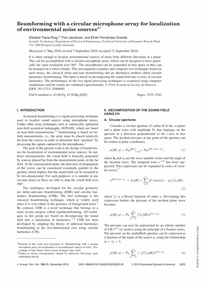
Beamforming with a circular microphone array for localizationof environmental noise sourcesa)
Elisabet Tiana-Roig,b) Finn Jacobsen, and Efren Fernandez GrandeAcoustic Technology, Department of Electrical Engineering, Technical University of Denmark, Ørsteds Plads352, 2800 Kongens Lyngby, Denmark
(Received 11 May 2010; revised 7 September 2010; accepted 13 September 2010)
It is often enough to localize environmental sources of noise from different directions in a plane.
This can be accomplished with a circular microphone array, which can be designed to have practi-
cally the same resolution over 360�. The microphones can be suspended in free space or they can
be mounted on a solid cylinder. This investigation examines and compares two techniques based on
such arrays, the classical delay-and-sum beamforming and an alternative method called circular
harmonics beamforming. The latter is based on decomposing the sound field into a series of circular
harmonics. The performance of the two signal processing techniques is examined using computer
simulations, and the results are validated experimentally.VC 2010 Acoustical Society of America.[DOI: 10.1121/1.3500669]
PACS number(s): 43.60.Fg, 43.50.Rq [EJS] Pages: 3535–3542
I. INTRODUCTION
Acoustical beamforming is a signal processing technique
used to localize sound sources using microphone arrays.
Unlike other array techniques such as statistically optimized
near-field acoustical holography (SONAH), which are based
on near-field measurements,1,2 beamforming is based on far-
field measurements, i.e., the array must be placed relatively
far from the sources in order to determine their “position” by
processing the signals captured by the microphones.3
The goal of the present work is the design of beamform-
ers for localization of environmental noise sources. In out-
doors measurements, the sound field is basically generated
by sources placed far from the measurement point, in the far
field. At the measurement point, the direction of propagation
of the waves can be considered essentially parallel to the
ground, which implies that the sound field can be assumed to
be two-dimensional. For such purposes, it is suitable to use
circular arrays as these are able to map the sound field over
360�.The techniques developed for the circular geometry
are delay-and-sum beamforming (DSB) and circular har-
monics beamforming (CHB). The first technique is the
classical beamforming technique, which is widely used
since it is very robust in the presence of background noise.4
By contrast, CHB is a novel technique that belongs to a
more recent category called eigenbeamforming. All techni-
ques in this group are based on decomposing the sound
field into a summation of harmonics.5–8 CHB has been
developed by adapting the theory of spherical harmonics
beamforming to the two-dimensional case using circular
harmonics (CH).
II. DECOMPOSITION OF THE SOUND FIELDUSING CH
A. Circular apertures
Consider a circular aperture of radius R in the xy-planeand a plane wave with amplitude P0 that impinges on the
aperture in a direction perpendicular to the z-axis in free
space. The incident pressure at any point of the aperture can
be written in polar coordinates,
pðkR;uÞ ¼ P0ejki�r��
r¼R¼ P0e
jkR cosðu�uiÞ; (1)
where ki and ui are the wave number vector and the angle of
the incident wave. The temporal term e�jxt has been sup-
pressed. This expression can be expanded in series of circu-
lar waves,9
ejkR cosðu�uiÞ ¼ J0ðkRÞ þX1n¼1
2jn cosðnðu� uiÞÞ JnðkRÞ;
(2)
where Jn is a Bessel function of order n. Developing this
expression further, the pressure of the incident plane wave
becomes
pðkR;uÞ ¼ P0
X1n¼�1
jnJnðkRÞejnðu�uiÞ: (3)
The pressure can now be represented by an infinite number
of CH ejnu (or modes) using the principle of a Fourier series.
The pressure on the (unbaffled) aperture can be expressed as
a function of the angle of the source us using the relationship
ui ¼ us þ p,
pðkR;uÞ ¼ P0
X1n¼�1
ð�jÞnJnðkRÞejnðu�usÞ: (4)b)Author to whom correspondence should be addressed. Electronic mail:
a)Portions of this work were presented in “Beamforming with a circular
microphone array for localization of environmental sources of noise,” Pro-
ceedings of Inter-Noise 2010, Lisbon, Portugal, June 2010.
J. Acoust. Soc. Am. 128 (6), December 2010 VC 2010 Acoustical Society of America 35350001-4966/2010/128(6)/3535/8/$25.00
Aut
hor's
com
plim
enta
ry c
opy

When the same aperture is mounted on a rigid, infinite
cylinder, the incident wave is scattered by the cylinder. The
pressure on the baffled aperture is the superposition of
the incident pressure and the scattered pressure, p ¼ pi þ ps.The scattered pressure at positions on the aperture becomes10
psðkR;uÞ ¼X1n¼0
An cosðnuÞðJnðkRÞ þ jYnðkRÞÞ; (5)
where the terms An are a set of coefficients and Yn is a Neu-mann function of order n. Making use of the Hankel func-
tions of first kind, Hn(�) ¼ Jn(�) þ jYn(�), the previous
expression can be rewritten as
psðkR;uÞ ¼X1
n¼�1BnHnðkRÞejnu: (6)
The terms Bn are obtained by imposing that the total velocity
in the radial direction vanishes on the surface of the rigid
cylinder, ui,r þ us,r ¼ 0,
Bn ¼ �P0ð�jÞn J0nðkRÞ
H0nðkRÞ
e�jnus ; (7)
where J0n and H0n are the derivatives of the Bessel and Hankel
functions with respect to the radial dimension. Using the expres-
sions given in Eqs. (4) and (6) for the incident and the scattered
wave, together with the coefficients obtained in Eq. (7), the total
pressure at the surface of the rigid cylinder becomes
pðkR;uÞ ¼ P0
X1n¼�1
ð�jÞn
� JnðkRÞ � J0nðkRÞHnðkRÞH0
nðkRÞ� �
ejnðu�usÞ: (8)
Comparing Eqs. (3) and (8) with a Fourier series in the
exponential form11 shows that the pressure on the baffled or
the unbaffled apertures can be represented as
pðkR;uÞ ¼X1n¼�1
Cnejnu; (9)
where the Fourier coefficients Cn for the two cases are
CnðkR;usÞ ¼ P0QnðkRÞe�jnus ; (10)
with
QnðkRÞ¼ð�jÞnJnðkRÞ unbaffled;
ð�jÞn JnðkRÞ� J0nðkRÞHnðkRÞH0
nðkRÞ� �
baffled:
8<: (11)
The modulus of the first four coefficients Cn is shown in
Fig. 1, for baffled and unbaffled apertures. At low values of
kR, the zero order mode is constant and equals 0 dB in both
cases, whereas all the other modes have a slope of 10 � n dB
per decade. When the aperture is baffled, the response is
offset by 6 dB compared with the unbaffled case. With
increasing values of kR, more and more harmonics gain
strength. However, for the unbaffled aperture the response
exhibits some dips that imply that signals that have compo-
nents around these dips cannot be totally resolved. This prob-
lem disappears when the cylindrical baffle is used.
Since the curves of the Fourier coefficients are functions
of kR, variation of R implies that the curves are scaled in fre-
quency (or wave number), and vice-versa. For instance,
when R is increased, the response is shifted toward low fre-
quencies, whereas a decrease of R results in a shift toward
high frequencies.
B. Implementation using microphone arrays
In principle, infinitely many Fourier terms are needed to
represent the sound pressure. However, in practice the num-
ber of harmonics must be truncated to a maximum order, N.As a rule of thumb,
N � kR (12)
is usually chosen as a first approximation.8,12,13 The reason
for this is that the amplitude of the Bessel functions in the
Fourier coefficients [see Eqs. (10) and (11)] is small when
the order of the Bessel functions n exceeds its argument
(kR). Thus, the overall contribution of modes jnj > kR is
very small.
Besides, microphone arrays rather than “ideal” continu-
ous apertures are used in real-life applications, which implies
FIG. 1. (Color online) Normalized modulus of the four lowest Fourier coef-
ficients of the pressure on an unbaffled circular aperture (top) and on a circu-
lar aperture mounted on a rigid cylindrical baffle of infinite length (bottom).
3536 J. Acoust. Soc. Am., Vol. 128, No. 6, December 2010 Tiana-Roig et al.: Beamforming with a circular microphone array
Aut
hor's
com
plim
enta
ry c
opy

that apertures are sampled at discrete points. Assuming that
an aperture is sampled with M omnidirectional microphones
placed equidistantly, the Fourier coefficients become
~Cn ¼ 1
M
XMm¼1
~pðkR;umÞe�jnum ; (13)
where ~p is the measured pressure at the mth microphone
placed at an angle um.
The sampling procedure introduces an error in the Fou-
rier coefficients. For example, it can be shown that in the
case of an unbaffled circular array, the Fourier coefficients
resulting after the sampling are, theoretically,12–14
~CnðkRÞ ¼ P0ð�jÞnJnðkRÞe�jnus
þ P0
X1q¼1
ð�jÞgJgðkRÞejgus
þ P0
X1q¼1
ð�jÞhJhðkRÞejhus ; (14)
where g ¼ Mq � n and h ¼ Mq þ n. Note that the first termis identical to the Fourier coefficient of the continuous aper-
ture; see Eq. (10), whereas the remaining terms are residuals
caused by the sampling. Further examination of Eq. (14)
reveals that the first term is the dominant one when M> 2jnj. Since the highest mode excited is N,
M > 2N: (15)
In fact, inserting the approximation for N given in Eq.
(12) into Eq. (15) yields the Nyquist sampling criterion:
M > 2kR ) M > 22pkR ) k
2> d; (16)
where k is the wavelength and d is the distance between two
consecutive microphones. Hence, by fulfilling the relation-
ship between M and N given in Eq. (15), the Nyquist crite-
rion is satisfied.14
III. BEAMFORMING TECHNIQUES
A. CHB
The beamformer response is the output of the beam-
former as a function of the steering angle, i.e., the angle at
which the main beam of the beamformer is pointing. Ideally,
the beamformer response should assume a maximum when
the beamformer is steered toward the source at us, and
should be zero in all other directions; that is,
bidealðuÞ ¼ Adðu� usÞ; (17)
where A is a scale factor. This can be described in terms of a
Fourier series,
bidealðuÞ ¼X1n¼�1
Inejnu; (18)
In ¼ 1
2p
ð2p0
bidealðuÞe�jnu du ¼ Ae�jnus : (19)
It follows that
bidealðuÞ ¼ AX1n¼�1
e�jnus ejnu: (20)
Using Eq. (10), the output of the ideal beamformer
becomes
bidealðkR;uÞ ¼ AX1
n¼�1
CnðkR;usÞP0QnðkRÞ e
jnu: (21)
In real implementations, the number of modes must be
truncated at a reasonable value, N, and the aperture must be
sampled by a number of microphones, M. Thus
bN;CHðkR;uÞ ¼ AXNn¼�N
~CnðkR;usÞP0QnðkRÞ e
jnu: (22)
Comparing with Eq. (10), Eq. (22) be rewritten as
bN;CHðkR;uÞ ¼ AXNn¼�N
~CnðkR;usÞCnðkR;uÞ : (23)
When the beamformer is steered toward the position of
the source, u equals us, so the quotients approximate unity
and the output assumes a maximum. Note that, when using
unbaffled arrays, Eq. (23) has singularities at the frequencies
where the Fourier coefficients have dips; see Fig. 1. At such
frequencies, the CH beamformer is not capable of resolving
the location of the source properly.
Inserting the approximated coefficients given by Eq.
(13) into Eq. (22), the CH beamformer output becomes
bN;CHðkR;uÞ
¼ A
MP0
XMm¼1
~pðkR;umÞXNn¼�N
1
QnðkRÞ e�jnðum�uÞ
!: (24)
Ideally, this should be zero at all angles different from
us. However, since a limited number of microphones are
used, the response exhibits a main lobe around us and side
lobes at other angles.
B. DSB
The delay-and-sum (DS) technique aligns the signals
from the microphones of the array by introducing appropri-
ate delays and finally adds them together.3,15,16 The delays
are determined by the steering direction of the array. The
output assumes its maximum when the focusing direction
coincides with the position of the source.
In this investigation, the output of a DS beamformer is
implemented in the frequency domain using matched field
J. Acoust. Soc. Am., Vol. 128, No. 6, December 2010 Tiana-Roig et al.: Beamforming with a circular microphone array 3537
Aut
hor's
com
plim
enta
ry c
opy

processing. This method uses phase shifts to align the signals
in phase. Assuming that the beamformer is steered toward
the direction u, the beamformer output is
bDSðkR;uÞ ¼ AXMm¼1
wm~pðkR;umÞ � p�ðkR;um;uÞ; (25)
where
(1) wm is the weighting coefficient of the mth microphone;
(2) ~pðkR;umÞ is the pressure measured at the mth micro-
phone position due to a plane wave generated by a
source at us; and
(3) p�(kR,um,u) is the theoretical complex conjugated pres-
sure that would be captured at the mth microphone due
to plane wave generated at u. Note that the argument uis used to emphasize that this is the variable that defines
the focusing direction of the beamformer.
In general, the source position is unknown, and there-
fore the beamformer must map over all possible source posi-
tions, i.e., 0 � u < 2p. The key point is that when the
beamformer is focused toward the position of the source us,
the second and the third terms of Eq. (25) become equal in
magnitude but opposite in phase. In these circumstances, the
microphone signals are aligned in time, and therefore the
maximum output of the beamformer is reached.
In the case of an unbaffled array, the theoretical pressure
is simply the closed form for a plane wave, so the beam-
former output is
bDSðkR;uÞ ¼ AXMm¼1
wm~pðkR;umÞP0e�jki�r
�����r¼R
¼ AP0
M
XMm¼1
~pðkR;umÞejkR cosðum�uÞ: (26)
Since all microphones have equal “importance,” the
weights wm have been set to 1/M. For the baffled array, the
output of the beamformer is obtained by introducing Eq. (9)
into Eq. (25), and taking into account that the number of
modes used for the processing is truncated at a number N,
bN;DSðkR;uÞ
¼ AP0
M
XMm¼1
~pðkR;umÞXNn¼�N
Q�nðkRÞe�jnðum�uÞ
!: (27)
This expression is also valid for the unbaffled case,
although it is not as precise as Eq. (26) because of the
truncation.
Further analysis of Eq. (27) reveals that the beamformer
output can be written, according to Eqs. (10) and (13), as
bN;DSðkR;uÞ ¼ AXNn¼�N
~CnðkR;usÞ � C�nðkR;uÞ: (28)
As opposed to CHB, where the beamformer output could
be expressed as the ratio of the approximated coefficients to
the theoretical ones [see Eq. (23)], the output of the DS
beamformer is a multiplication of these terms. Therefore, in
the case of unbaffled arrays, the singularities that can be pres-
ent in CHB because of the dips of the Fourier coefficients are
totally resolved with a DS beamformer.
C. Beamformer performance—Resolution andmaximum side lobe level (MSL)
The resolution of a beamformer is defined as the �3 dB
width of the main lobe of the beampattern. This parameter is
of interest because it gives an approximation to the minimum
angular difference between two incoherent sources that is
necessary in order to distinguish them from each other.
The beamformer output will usually exhibit side lobes.
This is an unwanted effect as the beamformer seems to be
sensitive not only in the focusing direction but also in the
direction of the side lobes. Therefore, it is convenient to
evaluate the beamformer response by means of the MSL.
This parameter is the difference in level between the peak of
the highest side lobe and the peak of the main lobe.
IV. SIMULATIONS
The performance of circular arrays with CHB and DSB
has been evaluated by means of simulations. The circular
arrays have radii of 10 and 20 cm and 10 and 20 microphones,
respectively. The number of microphones and the radius of
each array were chosen by setting the same maximum fre-
quency that could be represented without any sampling error
(around 2.7 kHz); see Sec. II B. The simulations were carried
out under ideal conditions, i.e., without background noise.
The source was placed at 180�, but the source position has a
very limited influence on the results. The amplitude of the
waves impinging on the array was the same at all frequencies.
A. Simulations with CHB
The resolution and the MSL obtained with CHB and an
unbaffled circular array are shown in Fig. 2, for the range
from 50 Hz to 3.5 kHz. The number of orders used in the
CHB algorithm given in Eq. (24) followed N ¼ dkRe, whered�e is the ceiling function. The maximum value of N was
M/2 � 1 in order to fulfill Eq. (15).
As can be seen, the resolution and the MSL are constant
for a certain interval. This depends on the number of orders
N used for the processing. The fact that the main lobe
becomes narrower from interval to interval indicates an
improvement in the resolution. More intervals, i.e., more
orders, result in a better resolution, which is the case of the
array of largest radius. The MSL follows the same behavior
as the resolution, improving when the number of orders is
increased. The staircase pattern in these two measures is also
obtained with spherical harmonics beamforming.
At some frequencies an “unexpected” response occurs,
e.g., around 2.1 kHz for the array of 10 cm and 2.8 kHz for
the array of 20 cm. This phenomenon is due to the dips
in the Fourier coefficients obtained with unbaffled arrays.
The frequencies where this phenomenon occurs cannot be
resolved as precisely as the neighboring frequencies. This
3538 J. Acoust. Soc. Am., Vol. 128, No. 6, December 2010 Tiana-Roig et al.: Beamforming with a circular microphone array
Aut
hor's
com
plim
enta
ry c
opy

effect is avoided when the array is mounted on a rigid cylin-
drical baffle. The overall behavior of the CH beamformers
when baffled arrays are used is very similar to the unbaffled
case but without the problem of unresolved frequencies.
The arrays can be used up to a maximum frequency
without any sampling error. For the arrays under analysis,
this occurs at about 2.7 kHz. Above this frequency, the effect
of the sampling error can be seen especially in the MSL (the
magnitude of the side lobes is higher than in the previous
interval of frequencies).
B. Simulations with DSB
The resolution and the MSL obtained under ideal condi-
tions using DSB are shown in Fig. 3 for both baffled and
unbaffled arrays. In the case of baffled arrays, the number of
orders used in the DSB algorithm, stated in Eq. (27), was N¼ dkRe þ 1, up to a maximum N ¼ M/2 � 1 according to
Eq. (15).
It is apparent that the resolution is 360� at low frequen-
cies in all cases, and the MSL is non-existent, meaning that
the beamformer is omnidirectional. From a certain frequency
depending on the radius of the array, the resolution improves
continuously until high frequencies. The curves decay in a
similar way for both kinds of arrays, but in the baffled case
they exhibit small smooth fluctuations. The MSL curves
begin at a certain frequency and grow progressively until a
maximum level is reached. In the case of unbaffled arrays,
this level remains constant, whereas for baffled arrays the
MSL exhibits ripples while it increases toward high frequen-
cies. Nevertheless, the MSL is better for baffled arrays than
for unbaffled.
In both cases, the performance improves with increasing
radius of the array and is better in the case of baffled arrays.
Furthermore, it can be seen that the baffled array of 10 cm of
radius has resolution and MSL similar to the unbaffled array
of radius 20 cm. Thus it can be concluded that mounting an
array on an infinite baffle makes it seem to be “larger” than
in the unbaffled case. Similar characteristics are found when
DSB is applied to spherical arrays.
In general the resolution obtained with DSB is much
worse than the resolution obtained with CHB. At high fre-
quencies, the MSL with DSB is worse than with CHB for
unbaffled arrays; but the opposite is the case for baffled arrays.
V. EXPERIMENTAL RESULTS
A prototype array with a radius of 11.9 cm has been
tested in an anechoic room with a volume of about 1000 m3.
The array was constructed by mounting twelve 1/4 in. micro-
phones, Bruel & Kjær (B&K) Type 4935, on a circular
frame, corresponding to a microphone for every 30�. Theimplemented prototype is shown in Fig. 4.
The array and the source, a loudspeaker, were controlled
by a B&K PULSE Analyzer. In all the measurements the
loudspeaker was driven by a signal from the generator, pseu-
dorandom noise of 1 s of period, 3.2 kHz of bandwidth, and
1 Hz of resolution. The microphones signals were recorded
with the analyzer and postprocessed with the beamforming
algorithms DSB and CHB.
The normalized outputs obtained with both CHB and
DSB are shown on top of Fig. 5, whereas the simulated out-
puts are provided in the bottom. To account for the back-
ground noise introduced in the measurements, the
simulations were carried out with a signal-to-noise ratio
(SNR) of 30 dB at the input of each microphone due to uni-
formly distributed noise.
FIG. 2. Resolution and MSL using CHB and unbaffled arrays of radii 10
and 20 cm and 10 and 20 microphones, respectively. The source is placed
at 180�.
FIG. 3. Resolution and MSL using DSB and circular arrays of radius 10 and
20 cm and 10 and 20 microphones, respectively. Solid lines: Unbaffled
arrays; dashed lines: Baffled arrays. The source is placed at 180�.
J. Acoust. Soc. Am., Vol. 128, No. 6, December 2010 Tiana-Roig et al.: Beamforming with a circular microphone array 3539
Aut
hor's
com
plim
enta
ry c
opy
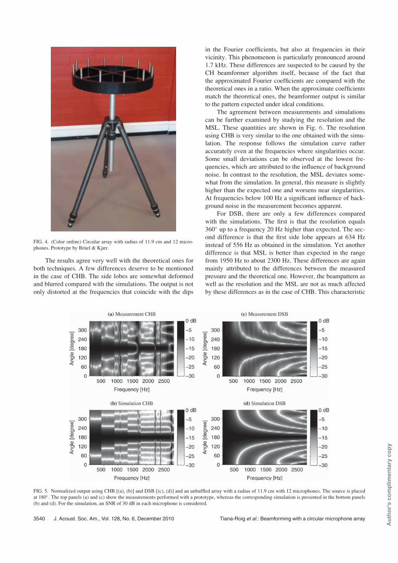
The results agree very well with the theoretical ones for
both techniques. A few differences deserve to be mentioned
in the case of CHB. The side lobes are somewhat deformed
and blurred compared with the simulations. The output is not
only distorted at the frequencies that coincide with the dips
in the Fourier coefficients, but also at frequencies in their
vicinity. This phenomenon is particularly pronounced around
1.7 kHz. These differences are suspected to be caused by the
CH beamformer algorithm itself, because of the fact that
the approximated Fourier coefficients are compared with the
theoretical ones in a ratio. When the approximate coefficients
match the theoretical ones, the beamformer output is similar
to the pattern expected under ideal conditions.
The agreement between measurements and simulations
can be further examined by studying the resolution and the
MSL. These quantities are shown in Fig. 6. The resolution
using CHB is very similar to the one obtained with the simu-
lation. The response follows the simulation curve rather
accurately even at the frequencies where singularities occur.
Some small deviations can be observed at the lowest fre-
quencies, which are attributed to the influence of background
noise. In contrast to the resolution, the MSL deviates some-
what from the simulation. In general, this measure is slightly
higher than the expected one and worsens near singularities.
At frequencies below 100 Hz a significant influence of back-
ground noise in the measurement becomes apparent.
For DSB, there are only a few differences compared
with the simulations. The first is that the resolution equals
360� up to a frequency 20 Hz higher than expected. The sec-
ond difference is that the first side lobe appears at 634 Hz
instead of 556 Hz as obtained in the simulation. Yet another
difference is that MSL is better than expected in the range
from 1950 Hz to about 2300 Hz. These differences are again
mainly attributed to the differences between the measured
pressure and the theoretical one. However, the beampattern as
well as the resolution and the MSL are not as much affected
by these differences as in the case of CHB. This characteristic
FIG. 4. (Color online) Circular array with radius of 11.9 cm and 12 micro-
phones. Prototype by Bruel & Kjær.
FIG. 5. Normalized output using CHB [(a), (b)] and DSB [(c), (d)] and an unbaffled array with a radius of 11.9 cm with 12 microphones. The source is placed
at 180�. The top panels (a) and (c) show the measurements performed with a prototype, whereas the corresponding simulation is presented in the bottom panels
(b) and (d). For the simulation, an SNR of 30 dB in each microphone is considered.
3540 J. Acoust. Soc. Am., Vol. 128, No. 6, December 2010 Tiana-Roig et al.: Beamforming with a circular microphone array
Aut
hor's
com
plim
enta
ry c
opy

and the fact that the influence of background noise is lower
than CHB demonstrate that DSB is a more robust algorithm.
VI. CONCLUSIONS
Two different beamforming techniques based on circu-
lar arrays have been examined theoretically and experimen-
tally, CHB and the well-known DSB. CHB is an adaptation
of the spherical harmonics beamforming technique to a cir-
cular geometry.
The prototype used for the experimental investigation
gave very satisfactory results: The beampatterns, the resolu-
tion, and the MSL were found to be in extremely good agree-
ment with simulations for both CHB and DSB.
For a given array, CHB has better resolution and lower
MSL in a wider frequency range than DSB has. Regardless
of the technique, these quantities improve with increasing
frequency. The frequency range is limited at low frequencies
by the influence of background noise in the case of CHB and
by the fact that the output becomes omnidirectional for DSB.
At high frequencies, the limitation is in both cases given by
the increase of the sampling error.
Keeping the number of microphones constant, the beam-
former response is scaled in frequency when the radius of the
array is modified. However, when the radius of the array is
kept constant but the number of microphones is increased,
the response improves toward higher frequencies since the
spacing between the microphones becomes smaller. In fact,
by increasing the number of microphones, the array behaves
more similarly to a continuous aperture.
A given ratio between the number of microphones and
the radius of the array determines the upper frequency above
which a sampling error occurs. In such case, the overall per-
formance improves considerably toward lower frequencies
when increasing the radius. However, the number of micro-
phones should be increased accordingly, otherwise the upper
limit frequency would be reduced.
In the presence of background noise, DSB is more robust
than CHB, and CH beamformers exhibit singularities, i.e., fre-
quencies that cannot properly be resolved, when unbaffled cir-
cular arrays are used. This problem would be solved if it were
feasible to mount the arrays on rigid cylindrical baffles of infi-
nite length. The performance of DS beamformers would also
improve substantially by mounting the arrays on rigid cylin-
drical baffles of infinite length, but this is not realistic.
CHB can be used in the entire frequency range except at
the frequencies that cannot be properly resolved due to the
nature of this technique. At such frequencies, it is convenient
to use DSB instead. In addition to this, DSB should not be
underestimated in environments with a poor SNR because of
its robustness.
ACKNOWLEDGMENTS
The authors would like to thank Karim Haddad and Jørgen
Hald, Bruel & Kjær, for lending us a circular microphone array
and other equipment for the beamforming measurements. We
would also like to thank Julien Jourdan and Marton Marschall
for their notes about spherical harmonics beamforming, which
became very helpful for the present work.
1J. Maynard, E. Williams, and Y. Lee, “Nearfield acoustic holography:
I. Theory of generalized holography and the development of NAH,”
J. Acoust. Soc. Am. 78(4), 1397–1413 (1985).2J. Hald, “Basic theory and properties of statistically optimized near-field
acoustical holography,” J. Acoust. Soc. Am. 125(4), 2105–2120 (2009).3J. Hald, “Beamforming and wavenumber processing,” in Handbook of Sig-nal Processing in Acoustics, edited by D. Havelock, S. Kuwano, and M.
Vorlander (Springer, New York, 2008), Chap. 9, pp. 131–144.
FIG. 6. Resolution and MSL using CHB (left) and DSB (right) and an unbaffled array with a radius of 11.9 cm with 12 microphones. The source is placed at
180�. The theoretical case obtained by simulation is also shown. The SNR in each microphone is set to 30 dB for the simulation.
J. Acoust. Soc. Am., Vol. 128, No. 6, December 2010 Tiana-Roig et al.: Beamforming with a circular microphone array 3541
Aut
hor's
com
plim
enta
ry c
opy
4J. Bitzer and K. Uwe Simmer, “Superdirective microphone arrays,” in
Microphone Arrays. Signal Processing Techniques and Applications,edited by M. Brandstein and D. Ward (Springer, Berlin, 2001), Chap. 2,
p. 26.5B. Rafaely, “Plane-wave decomposition of the sound field on a sphere by
spherical convolution,” J. Acoust. Soc. Am. 116(4), 2149–2157 (2004).6W. Song, W. Ellermeier, and J. Hald, “Using beamforming and binaural
synthesis for the psychoacoustical evaluation of target sources in noise,”
J. Acoust. Soc. Am. 123(2), 910–924 (2008).7H. Teutsch and W. Kellermann, “Acoustic source detection and localiza-
tion based on wavefield decomposition using circular microphone arrays,”
J. Acoust. Soc. Am. 120(5), 2724–2736 (2006).8H. Teutsch, Modal Array Signal Processing: Principles and Applicationsof Acoustic Wavefield Decomposition (Springer, Berlin, 2007), pp. 150–
188.9P. Morse and H. Feshbach,Methods of Theoretical Physics (McGraw-Hill,
New York, 1953), Vol. I, p. 828.
10P. Morse, Vibration and Sound, 2nd ed. (McGraw-Hill, New York, 1948),
pp. 347–348.11E. Williams, Fourier Acoustics: Sound Radiation and Nearfield AcousticHolography (Academic Press, London, 1999), pp. 4–5.
12C. Mathews and M. Zoltowski, “Eigenstructure techniques for 2-D angle
estimation with uniform circular arrays,” IEEE Trans. Signal Process.
42(9), 2395–2407 (1994).13D. E. N. Davies, “Circular arrays,” in The Handbook of Antenna Design,edited by A. W. Rudge, K. Milne, A. D. Olver, and P. Knight (Peter Pere-
grinus Ltd., London, 1983), Vol. II, Chap. 12, pp. 298–310.14H. Van Trees, Optimum Array Processing. Part IV of Detection, Estima-tion, and Modulation Theory (Wiley, New York, 2002), pp. 280–284.
15D. Johnson and D. Dudgeon, Array Signal Processing Concepts and Tech-niques (Prentice Hall, Englewood Cliffs, NJ, 1993), pp. 112–119.
16G. Elko and J. Meyer, “Microphone arrays,” in Springer Handbook ofSpeech Processing, edited by J. Benesty, M. Sondhi, and Y. Huang
(Springer-Verlag, Berlin, 2008), Chap. 50, pp. 1021–1042.
3542 J. Acoust. Soc. Am., Vol. 128, No. 6, December 2010 Tiana-Roig et al.: Beamforming with a circular microphone array
Aut
hor's
com
plim
enta
ry c
opy

Paper B


Beamforming with a circular array of microphones mountedon a rigid sphere (L)
Elisabet Tiana-Roig,a) Finn Jacobsen, and Efren Fernandez-GrandeAcoustic Technology, Department of Electrical Engineering, Technical University of Denmark, Ørsteds Plads352, 2800 Kongens Lyngby, Denmark
(Received 4 November 2010; revised 6 July 2011; accepted 7 July 2011)
Beamforming with uniform circular microphone arrays can be used for localizing sound sources
over 360�. Typically, the array microphones are suspended in free space or they are mounted on a
solid cylinder. However, the cylinder is often considered to be infinitely long because the scattering
problem has no exact solution for a finite cylinder. Alternatively one can use a solid sphere. This
investigation compares the performance of a circular array mounded on a rigid sphere with that of
such an array in free space and mounted on an infinite cylinder, using computer simulations. The
examined techniques are delay-and-sum and circular harmonics beamforming, and the results are
validated experimentally.VC 2011 Acoustical Society of America. [DOI: 10.1121/1.3621294]
PACS number(s): 43.60.Fg [EJS] Pages: 1095–1098
I. INTRODUCTION
During the past decade, studies on the performance of
circular arrays of microphones for localizing sound sources
over 360� have been reported. For example, Meyer1 utilized
modal beamforming to generate a desired beampattern for a
circular microphone array mounted around a rigid sphere.
Daigle et al.2 considered delay-and-sum beamforming with
circular arrays mounted on the surface of sound absorbing
spheres and cylinders and showed that the achieved beam-
width improved over that of arrays mounted on hard spheres
and cylinders. Instead of delay-and-sum beamforming,
Teutsch and Kellermann3 analyzed various algorithms based
on decomposing the sound field into a series of modes for a
circular array mounted on a cylinder. Still in the field of
modal beamforming Tiana-Roig et al.4 adapted the theory of
spherical harmonics beamforming to the two-dimensional
case using circular harmonics. The resulting circular har-
monics beamformer was compared to the classical delay-
and-sum beamformer using both a circular array suspended
in free space and one mounted on a rigid, infinite cylinder.
This letter to the editor repeats the comparison for the case
of a circular array mounted on a rigid sphere.
II. PLANE WAVE DECOMPOSITION
Consider a plane wave, ejki�r, generated by a source
placed in the far field, at a polar angle hs and azimuth angle
us, that impinges on a rigid sphere with radius R. The pres-
sure on the surface of the sphere, at a point with spherical
coordinates ½R; h;u, can be written as5,6
pðkR; h;uÞ ¼ 4pX1q¼0
bqðkRÞXqn¼�q
Ynqðh;uÞYn
qðhs;usÞ�; (1)
where
bqðkRÞ ¼ ð�jÞq jqðkRÞ �j0qðkRÞh0qðkRÞ
hqðkRÞ !
; (2)
Ynqðh;uÞ
ffiffiffiffiffiffiffiffiffiffiffiffiffiffiffiffiffiffiffiffiffiffiffiffiffiffiffiffiffiffiffiffiffiffið2qþ 1Þ
4pðq� nÞ!ðqþ nÞ!
sPnqðcos hÞejnu: (3)
In the function bn, which accounts for the effect of the rigid
scatterer, jq is a spherical Bessel function of order q, hq is a
spherical Hankel function of first kind and order q, and j0qand h0q are their derivatives. On the other hand, Yn
q is a spher-
ical harmonic, in which Pnq is a Legendre function of degree
q and order n. Note that in Eq. (1) the temporal term e�jxt is
omitted; and the angles of the position of the source ½hs;usare used instead of the angles of the incident wave ½hi;ui,these being related by hs ¼ p� hi and us ¼ ui þ p because
the unit vector of the incident wave ki is opposite to the unit
vector of the position of the source rs, ki ¼ �rs.Now a circular aperture of radius R is mounted at the
equator of the rigid sphere, in the xy plane. Because the polarangle at all positions of the aperture is constant, i.e.,
h ¼ p=2, its pressure can be represented in a Fourier series
in the u coordinate.5 The resulting Fourier coefficients are
Cn ¼ 1
2p
ð2p0
pðkR; p=2;uÞe�jnudu: (4)
Inserting Eq. (1), it can be shown that the coefficients
become
CnðkRÞ ¼X1q¼ nj j
ð2qþ 1ÞbnðkRÞ
� ðq� nj jÞ!ðqþ nj jÞ!P
nj jq ð0ÞP nj j
q ðcos hsÞe�jnus : (5)
Figure 1 shows the magnitude of the first four coefficients
assuming a source located in the plane of the aperture, i.e., at
hs ¼ p=2. The advantage of this configuration is that its
behavior resembles the one of a circular aperture mounted
a)Author to whom correspondence should be addressed. Electronic mail:
etr@elektro. dtu.dk
J. Acoust. Soc. Am. 130 (3), September 2011 VC 2011 Acoustical Society of America 10950001-4966/2011/130(3)/1095/4/$30.00
Aut
hor's
com
plim
enta
ry c
opy
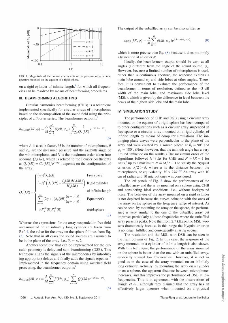
on a rigid cylinder of infinite length,4 for which all frequen-
cies can be resolved by means of beamforming procedures.
III. BEAMFORMING ALGORITHMS
Circular harmonics beamforming (CHB) is a technique
implemented specifically for circular arrays of microphones
based on the decomposition of the sound field using the prin-
ciples of a Fourier series. The beamformer output is4
bN;CHBðkR;uÞ ¼ A
M
XMm¼1
~pðkR;umÞXNn¼�N
1
QnðkRÞ e�jnðum�uÞ;
(6)
where A is a scale factor, M is the number of microphones, ~pand um are the measured pressure and the azimuth angle of
the mth microphone, and N is the maximum order taken into
account. QnðkRÞ, which is related to the Fourier coefficients
as QnðkRÞ ¼ CnðkRÞ=e�jnus , depends on the configuration of
the array:
QnðkRÞ¼
ð�jÞnJnðkRÞ Freespace
ð�jÞn JnðkRÞ�J0nðkRÞHnðkRÞH0
nðkRÞ� �
Rigidcylinder
of infinite lengthX1q¼ nj j
ð2qþ1ÞbnðkRÞðq� nj jÞ!ðqþ nj jÞ! Equatorof a
�Pnj jq ð0ÞP nj j
q ð0Þ rigidsphere
8>>>>>>>>>>><>>>>>>>>>>>:
(7)
Whereas the expressions for the array suspended in free field
and mounted on an infinitely long cylinder are taken from
Ref. 4, the value for the array on the sphere follows from Eq.
(5). Note that in all cases the sound sources are assumed to
be in the plane of the array, i.e., hs ¼ p=2.Another technique that can be implemented for the cir-
cular geometry is delay-and-sum beamforming (DSB). This
technique aligns the signals of the microphones by introduc-
ing appropriate delays and finally adds the signals together.7
Implemented in the frequency domain using matched field
processing, the beamformer output is4
bN;DSBðkR;uÞ ¼ A
M
XMm¼1
~pðkR;umÞXNn¼�N
Q�nðkRÞe�jnðum�uÞ:
(8)
The output of the unbaffled array can be also written as
bDSBðkR;uÞ ¼ A
M
XMm¼1
~pðkR;umÞejkR cosðum�uÞ; (9)
which is more precise than Eq. (8) because it does not imply
a truncation at an order N.Ideally, the beamformers output should be zero at all
angles u different from the angle of the sound source, us.
However, because a limited number of microphones is used,
rather than a continuous aperture, the response exhibits a
main lobe around us and side lobes at other angles. There-
fore, it is convenient to evaluate the performance of the
beamformer in terms of resolution, defined as the �3 dB
width of the main lobe, and maximum side lobe level
(MSL), which is given by the difference in level between the
peaks of the highest side lobe and the main lobe.
IV. SIMULATION STUDY
The performance of CHB and DSB using a circular array
mounted on the equator of a rigid sphere has been compared
to other configurations such as a circular array suspended in
free space or a circular array mounted on a rigid cylinder of
infinite length by means of computer simulations. The im-
pinging plane waves were perpendicular to the plane of the
array and were created by a source placed at hs ¼ 90� and
us ¼ 180�. (Note, however, that the azimuth angle has a very
limited influence on the results.) The maximum order of the
algorithms followed N � kR for CHB and N � kRþ 1 for
DSB,4 up to a maximum N ¼ M=2� 1 to satisfy the Nyquist
criterion: k=2 > d, where d is the distance between the
microphones, or equivalently, M > 2kR.8,9 An array with 10
cm of radius and 10 microphones was considered.
The left panels of Fig. 2 show the performances of the
unbaffled array and the array mounted on a sphere using CHB
and considering ideal conditions, i.e., without background
noise. The behavior of the array mounted on a rigid cylinder
is not depicted because the curves coincide with the ones of
the array on the sphere in the frequency range of interest. As
can be seen, by mounting the array on the sphere, the perform-
ance is very similar to the one of the unbaffled array but
improves particularly at those frequencies where the unbaffled
array presents peaks. Note that from 2.7 kHz on the MSL wor-
sens dramatically because in this range the Nyquist criterion
is no longer fulfilled and consequently aliasing occurs.
The resolution and the MSL with DSB can be seen in
the right column of Fig. 2. In this case, the response of the
array mounted on a cylinder of infinite length is also shown.
With this technique, the performance of the array mounted
on the sphere is better than the one with an unbaffled array,
especially toward low frequencies. However, it is not as
good as in the case of the array mounted on an infinitely
long cylinder. Actually, by mounting the array on a cylinder
or on a sphere, the apparent distance between microphones
increases, and this improves the performance of DSB at low
frequencies. This is in agreement with the observations of
Daigle et al., although they claimed that the array has an
effectively larger aperture when mounted on a physical
FIG. 1. Magnitude of the Fourier coefficients of the pressure on a circular
aperture mounted on the equator of a rigid sphere.
1096 J. Acoust. Soc. Am., Vol. 130, No. 3, September 2011 Tiana-Roig et al.: Letters to the Editor
Aut
hor's
com
plim
enta
ry c
opy

structure independently of the beamforming technique,2
whereas the present study has revealed that this is not the
case with CHB.
V. EXPERIMENTAL RESULTS
A circular array mounted on a rigid sphere has been
tested in an anechoic room. The prototype array consisted of
16 1/4 in. microphones, Bruel & Kjær (B&K) type 4958,
mounted on the equator of a rigid sphere with a radius of
9.75 cm, corresponding to a microphone for every 22:5�.With this configuration, the array can operate free of aliasing
up to about 4.5 kHz.
The array and the source, a loudspeaker, were controlled
by a B&K PULSE analyzer. The loudspeaker was driven by a
signal from the generator, pseudorandom noise of 1 s of pe-
riod, 6.4 kHz of bandwidth, and 1 Hz of resolution. The
microphone signals were recorded with the analyzer and post-
processed with the beamforming algorithms CHB and DSB.
Figure 3 shows the output of the array using CHB and
DSB when a source is located 4 m away but at the very same
height and at an azimuth angle us ¼ 180�. It can be seen that
with the two techniques, the array is capable of localizing
the sound source in the frequency range of interest with
exception of DSB at the frequencies below about 300 Hz
due to the fact that this technique behaves omnidirectionally
at such values.
The performance of the array is also illustrated in Fig. 4,
where the resolution and the MSL for both CHB and DSB
are shown. The predictions made with computer simulations
are also depicted. To account for the background noise intro-
duced in the measurements, the simulations were carried out
with a signal-to-noise ratio (SNR) of 30 dB at the input of
each microphone due to uniformly distributed noise.
FIG. 2. Resolution and MSL using CHB (left) and DSB (right) and a circular array of radius 10 cm and 10 microphones when the microphones are suspended
in free space, mounted on the equator of a rigid sphere, and mounted on a rigid cylinder of infinite length. For ease of comparison, the case of the cylinder
with CHB is not plotted because it coincides with the case of the sphere. In all cases, the source is in the far field at ½hs;us ¼ ½90�; 180�.
FIG. 3. Normalized output with CHB (left) and DSB (right) using a circular array with 16 microphones mounted on the equator of a rigid sphere with radius
of 9.75 cm. The source is in the far field at ½hs;us ¼ ½90�; 180�.
J. Acoust. Soc. Am., Vol. 130, No. 3, September 2011 Tiana-Roig et al.: Letters to the Editor 1097
Aut
hor's
com
plim
enta
ry c
opy
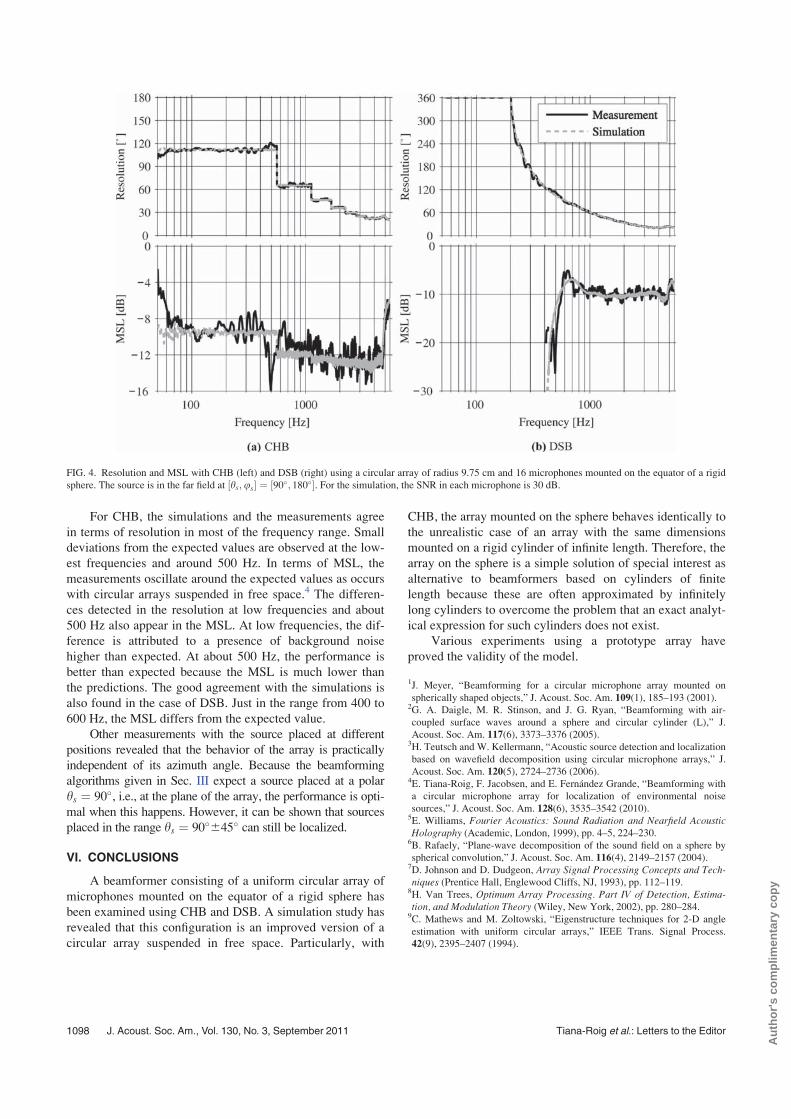
For CHB, the simulations and the measurements agree
in terms of resolution in most of the frequency range. Small
deviations from the expected values are observed at the low-
est frequencies and around 500 Hz. In terms of MSL, the
measurements oscillate around the expected values as occurs
with circular arrays suspended in free space.4 The differen-
ces detected in the resolution at low frequencies and about
500 Hz also appear in the MSL. At low frequencies, the dif-
ference is attributed to a presence of background noise
higher than expected. At about 500 Hz, the performance is
better than expected because the MSL is much lower than
the predictions. The good agreement with the simulations is
also found in the case of DSB. Just in the range from 400 to
600 Hz, the MSL differs from the expected value.
Other measurements with the source placed at different
positions revealed that the behavior of the array is practically
independent of its azimuth angle. Because the beamforming
algorithms given in Sec. III expect a source placed at a polar
hs ¼ 90�, i.e., at the plane of the array, the performance is opti-
mal when this happens. However, it can be shown that sources
placed in the range hs ¼ 90�645� can still be localized.
VI. CONCLUSIONS
A beamformer consisting of a uniform circular array of
microphones mounted on the equator of a rigid sphere has
been examined using CHB and DSB. A simulation study has
revealed that this configuration is an improved version of a
circular array suspended in free space. Particularly, with
CHB, the array mounted on the sphere behaves identically to
the unrealistic case of an array with the same dimensions
mounted on a rigid cylinder of infinite length. Therefore, the
array on the sphere is a simple solution of special interest as
alternative to beamformers based on cylinders of finite
length because these are often approximated by infinitely
long cylinders to overcome the problem that an exact analyt-
ical expression for such cylinders does not exist.
Various experiments using a prototype array have
proved the validity of the model.
1J. Meyer, “Beamforming for a circular microphone array mounted on
spherically shaped objects,” J. Acoust. Soc. Am. 109(1), 185–193 (2001).2G. A. Daigle, M. R. Stinson, and J. G. Ryan, “Beamforming with air-
coupled surface waves around a sphere and circular cylinder (L),” J.
Acoust. Soc. Am. 117(6), 3373–3376 (2005).3H. Teutsch and W. Kellermann, “Acoustic source detection and localization
based on wavefield decomposition using circular microphone arrays,” J.
Acoust. Soc. Am. 120(5), 2724–2736 (2006).4E. Tiana-Roig, F. Jacobsen, and E. Fernandez Grande, “Beamforming with
a circular microphone array for localization of environmental noise
sources,” J. Acoust. Soc. Am. 128(6), 3535–3542 (2010).5E. Williams, Fourier Acoustics: Sound Radiation and Nearfield AcousticHolography (Academic, London, 1999), pp. 4–5, 224–230.
6B. Rafaely, “Plane-wave decomposition of the sound field on a sphere by
spherical convolution,” J. Acoust. Soc. Am. 116(4), 2149–2157 (2004).7D. Johnson and D. Dudgeon, Array Signal Processing Concepts and Tech-niques (Prentice Hall, Englewood Cliffs, NJ, 1993), pp. 112–119.
8H. Van Trees, Optimum Array Processing. Part IV of Detection, Estima-tion, and Modulation Theory (Wiley, New York, 2002), pp. 280–284.
9C. Mathews and M. Zoltowski, “Eigenstructure techniques for 2-D angle
estimation with uniform circular arrays,” IEEE Trans. Signal Process.
42(9), 2395–2407 (1994).
FIG. 4. Resolution and MSL with CHB (left) and DSB (right) using a circular array of radius 9.75 cm and 16 microphones mounted on the equator of a rigid
sphere. The source is in the far field at ½hs;us ¼ ½90�; 180�. For the simulation, the SNR in each microphone is 30 dB.
1098 J. Acoust. Soc. Am., Vol. 130, No. 3, September 2011 Tiana-Roig et al.: Letters to the Editor
Aut
hor's
com
plim
enta
ry c
opy

Paper C


Deconvolution for the localization of sound sources usinga circular microphone arraya)
Elisabet Tiana-Roigb) and Finn JacobsenAcoustic Technology, Department of Electrical Engineering, Technical University of Denmark,Ørsteds Plads 352, DK-2800 Kongens Lyngby, Denmark
(Received 14 September 2012; revised 18 June 2013; accepted 10 July 2013)
During the last decade, the aeroacoustic community has examined various methods based on
deconvolution to improve the visualization of acoustic fields scanned with planar sparse arrays of
microphones. These methods assume that the beamforming map in an observation plane can be
approximated by a convolution of the distribution of the actual sources and the beamformer’s
point-spread function, defined as the beamformer’s response to a point source. By deconvolving the
resulting map, the resolution is improved, and the side-lobes effect is reduced or even eliminated
compared to conventional beamforming. Even though these methods were originally designed for
planar sparse arrays, in the present study, they are adapted to uniform circular arrays for mapping
the sound over 360�. This geometry has the advantage that the beamforming output is practically
independent of the focusing direction, meaning that the beamformer’s point-spread function is
shift-invariant. This makes it possible to apply computationally efficient deconvolution algorithms
that consist of spectral procedures in the entire region of interest, such as the deconvolution
approach for the mapping of the acoustic sources 2, the Fourier-based non-negative least squares,
and the Richardson–Lucy. This investigation examines the matter with computer simulations and
measurements.VC 2013 Acoustical Society of America. [http://dx.doi.org/10.1121/1.4816545]
PACS number(s): 43.60.Fg [BEA] Pages: 2078–2089
I. INTRODUCTION
Beamforming with phased arrays of microphones is a
well established method for visualization of sound fields.
However, because the sound field is mapped with a discrete
number of microphones, beamforming techniques present
intrinsic limitations, specifically the frequency dependence
of the array resolution and the appearance of side lobes that
contaminate the beamforming map with sometimes unex-
pected results.1 These two factors make it difficult to inter-
pret the map and therefore to visualize the actual sound field
accurately.
The focus of the present investigation is on the improve-
ment of the performance of uniform circular arrays (UCAs)
for mapping the sound field over 360� around the array to
localize sound sources in the far field. This array geometry
has lately been of interest in various studies about environ-
mental noise localization, conferencing, and measurements
in ducts among others; see, for instance, Refs. 2–9. It has
been shown that a better performance in terms of resolution
and level of the side lobes can be achieved by mounting the
array on a scatterer such as a sphere or a cylinder3,4,6 or by
designing other techniques than delay-and-sum (DS) beam-
forming, for example, circular harmonics (CH) beamform-
ing.5 Nevertheless these solutions are not sufficient to result
in a clear and unambiguous beamforming map.
In the recent years, the aeroacoustic community has sug-
gested various methods to improve the beamforming map in
two-dimensional (2D) imaging using planar sparse arrays to
map the sound field in a region parallel to the plane of the
array. These methods rely on the fact that the map is a convo-
lution of the acoustic sources and the beamformer’s point-
spread function (PSF), which is defined as the response of the
beamformer to a point source. By means of deconvolution,
the distribution of the sources can be recovered presenting a
better resolution and reduced (or even suppressed) side lobes
in comparison with direct beamforming. Examples of decon-
volution methods can be found in Refs. 10–12 for static
uncorrelated noise sources, in Refs. 13–15 for correlated
noise sources, and in Ref. 16 for moving sources. The main
problem is that these methods require a high computational
effort due to the fact that they are based on iterative algo-
rithms. To improve the efficiency, certain techniques use
spectral (Fourier-based) procedures for the deconvolution,
but these can only be applied when the beamformer’s PSF is
shift-invariant, that is, when the response of the beamformer
to a point source depends only on the distance between the
focusing point of the beamformer and the position of the
point source. However, for 2D imaging, the assumption that
the PSF is shift-invariant is only a good approximation when
the source region is small compared with the distance
between the array and the source. Therefore the use of such
deconvolution approaches is restricted to a small region in
space unless it is expanded to a larger (and 3D) region by
making use of a coordinate transformation.10,17,18
Interestingly, one could think of adapting the existing
deconvolution methods to a UCA to improve its perform-
ance. Contrary to the case of planar sparse arrays for which
a)Portions of this work were presented in “Acoustical source mapping based
on deconvolution approaches for circular microphone arrays,” Proceedings
of Inter-Noise 2011, Osaka, Japan, September 2011.b)Author to whom correspondence should be addressed. Electronic address:
2078 J. Acoust. Soc. Am. 134 (3), September 2013 0001-4966/2013/134(3)/2078/12/$30.00 VC 2013 Acoustical Society of America
Aut
hor's
com
plim
enta
ry c
opy

the PSF is shift-variant per se, beamformers based on UCAs
have a practically shift-invariant PSF along the region of
interest,2,19 i.e., 360�, and consequently this scenario seems
particularly adequate for the use of Fourier-based deconvolu-
tion methods. In the following, the main deconvolution
methods that rely on a shift-invariant PSF, namely, the
deconvolution approach for the mapping of the acoustic
sources 2 (DAMAS2), the Fourier-based non-negative least
squares (FFT-NNLS), and the Richardson–Lucy (RL) will
be reformulated for the case of plane waves impinging on a
UCA. The first method, DAMAS2, introduced by Dougherty
in Ref. 10, is an extension of DAMAS of Brooks and
Humphreys (Ref. 13). The second algorithm, FFT-NNLS,
was adapted from the classical NNLS procedures20 by
Ehrenfried and Koop in Ref. 11. Finally RL, which was ini-
tially developed by Richardson and Lucy (Refs. 21 and 22)
for image restoration in astronomy, was also adapted for
acoustical purposes in Ref. 11. All these methods will be
examined by means of computer simulations and experimen-
tal results.
II. CONVOLUTIONAL FORMULATION FOR UNIFORMCIRCULAR ARRAYS
A beamformer based on a UCA of microphones is capa-
ble of mapping the sound field over 360� in the plane of the
array to find the direction of sound sources located in that
plane. By electronically steering the beamformer, the sound
field is scanned in a grid of azimuth angles u, from 0 to
360�, to detect the propagating acoustic waves that impinge
on the array and thereby to identify the direction of the
sound sources that emit them. When a single source is pres-
ent, the beamformer output exhibits a main lobe around the
azimuth of the source, whereas other directions are contami-
nated with side lobes; see Fig. 1.
The characteristics of the beampattern, i.e., the shape of
the main lobe and the side lobes, are given by the beamform-
er’s PSF. This function was originally defined as the beam-
former response to a point source with unit strength at an
arbitrary position of a grid located in a plane parallel to the
array plane.10–12 However, this definition needs to be
reformulated for a UCA because the goal is to look into all
possible azimuth angles around a UCA beamformer instead
of looking to a plane parallel to the array.
In the current study, the sources are considered to be
sufficiently far from the array position, and therefore waves
captured by the array can be regarded to be planar. This
assumption implies that the direction of the waves can be
identified, although the distance to the sources that emit
them cannot be estimated—this would require a near-field
scenario. Under the plane wave assumption, the PSF can be
redefined as the beamformer response to a plane wave of
unit amplitude created by a source in the far field of the
array. Then in the presence of incoherent sources, the beam-
former output is related to the PSF as
bðuÞ ¼Xu02G
sðu0ÞHðuju0Þ; (1)
where sðu0Þ contains information regarding the direction and
the strength (at the array position) of a plane wave created
by a source located at an azimuth angle u0 contained on the
grid G, whereas Hðu ju0Þ is the PSF at u due to a source at
u0. From now on s will be referred to as the source
distribution.
From this expression, it becomes apparent that the infor-
mation regarding sound sources can be recovered from the
measured beamformer map and the beamformer’s PSF. This
is done by means of a deconvolution procedure, imposing
that the distribution of sound sources must be non-negative
[sðu0Þ � 0]. This is an inverse problem, which in matrix
notation can be rewritten as
b ¼ Hs; (2)
where the vectors b and s contain the information about the
beamformer output and the source distribution, respectively,
and H is a matrix that in each column contains the PSF for
one source located at an angle u0 of the grid. Often the ma-
trix H can be singular, which implies that there may be infin-
itely many solutions for s.11
For a beamformer based on a UCA, the focusing direc-
tion can be steered to any position in the plane where the
array lies without changing the beampattern significantly
due to the symmetry of the array.2,19 This implies that the
overall shape of the beamformer’s PSF remains practically
the same independently of its looking direction as shown in
Fig. 2. A PSF that satisfies this condition is called to be
shift-invariant because it depends only on the difference of
the actual focus point u and the azimuth of a source u0,
Hðuju0Þ ¼ Hðu� u0Þ: (3)
Inserting this property into Eq. (1) leads to
bðuÞ ¼Xu02G
sðu0ÞHðu� u0Þ; (4)
which corresponds to a discrete circular convolution of sðuÞand HðuÞ. Making use of the convolution theorem, Eq. (3)
can be expressed with the discrete Fourier transform,FIG. 1. Illustration of beamforming with a UCA for detecting the location
of a distant sound source.
J. Acoust. Soc. Am., Vol. 134, No. 3, September 2013 E. Tiana-Roig and F. Jacobsen: Deconvolution for a circular microphone array 2079
Aut
hor's
com
plim
enta
ry c
opy
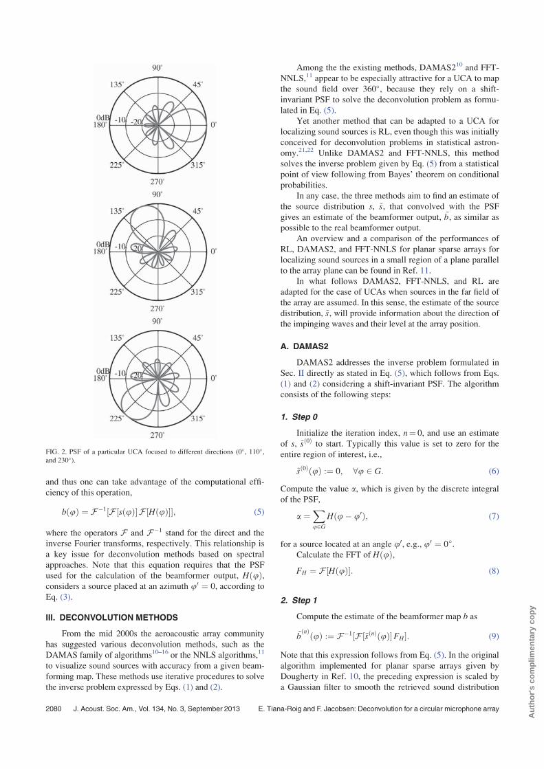
and thus one can take advantage of the computational effi-
ciency of this operation,
bðuÞ ¼ F�1½F ½sðuÞ F ½HðuÞ; (5)
where the operators F and F�1 stand for the direct and the
inverse Fourier transforms, respectively. This relationship is
a key issue for deconvolution methods based on spectral
approaches. Note that this equation requires that the PSF
used for the calculation of the beamformer output, HðuÞ,considers a source placed at an azimuth u0 ¼ 0, according to
Eq. (3).
III. DECONVOLUTION METHODS
From the mid 2000s the aeroacoustic array community
has suggested various deconvolution methods, such as the
DAMAS family of algorithms10–16 or the NNLS algorithms,11
to visualize sound sources with accuracy from a given beam-
forming map. These methods use iterative procedures to solve
the inverse problem expressed by Eqs. (1) and (2).
Among the the existing methods, DAMAS210 and FFT-
NNLS,11 appear to be especially attractive for a UCA to map
the sound field over 360�, because they rely on a shift-
invariant PSF to solve the deconvolution problem as formu-
lated in Eq. (5).
Yet another method that can be adapted to a UCA for
localizing sound sources is RL, even though this was initially
conceived for deconvolution problems in statistical astron-
omy.21,22 Unlike DAMAS2 and FFT-NNLS, this method
solves the inverse problem given by Eq. (5) from a statistical
point of view following from Bayes’ theorem on conditional
probabilities.
In any case, the three methods aim to find an estimate of
the source distribution s, ~s, that convolved with the PSF
gives an estimate of the beamformer output, ~b, as similar as
possible to the real beamformer output.
An overview and a comparison of the performances of
RL, DAMAS2, and FFT-NNLS for planar sparse arrays for
localizing sound sources in a small region of a plane parallel
to the array plane can be found in Ref. 11.
In what follows DAMAS2, FFT-NNLS, and RL are
adapted for the case of UCAs when sources in the far field of
the array are assumed. In this sense, the estimate of the source
distribution, ~s, will provide information about the direction of
the impinging waves and their level at the array position.
A. DAMAS2
DAMAS2 addresses the inverse problem formulated in
Sec. II directly as stated in Eq. (5), which follows from Eqs.
(1) and (2) considering a shift-invariant PSF. The algorithm
consists of the following steps:
1. Step 0
Initialize the iteration index, n¼ 0, and use an estimate
of s, ~sð0Þ to start. Typically this value is set to zero for the
entire region of interest, i.e.,
~sð0ÞðuÞ :¼ 0; 8u 2 G: (6)
Compute the value a, which is given by the discrete integral
of the PSF,
a ¼Xu2G
Hðu� u0Þ; (7)
for a source located at an angle u0, e.g., u0 ¼ 0�.Calculate the FFT of HðuÞ,FH ¼ F½HðuÞ: (8)
2. Step 1
Compute the estimate of the beamformer map b as
~bðnÞðuÞ :¼ F�1½F ½~sðnÞðuÞFH: (9)
Note that this expression follows from Eq. (5). In the original
algorithm implemented for planar sparse arrays given by
Dougherty in Ref. 10, the preceding expression is scaled by
a Gaussian filter to smooth the retrieved sound distribution
FIG. 2. PSF of a particular UCA focused to different directions (0�, 110�,and 230�).
2080 J. Acoust. Soc. Am., Vol. 134, No. 3, September 2013 E. Tiana-Roig and F. Jacobsen: Deconvolution for a circular microphone array
Aut
hor's
com
plim
enta
ry c
opy

and to minimize the influence of high wave-number noise,
i.e., background noise induced by sources outside the region
of interest.11 However, for the case of UCAs, this filter is not
necessary as all sources are placed inside the entire region of
interest, between 0� and 360�.
3. Step 2
Apply a non-negativity constraint to update the value of ~s
~sðnþ1ÞðuÞ :¼ max ~sðnÞðuÞ þ bðuÞ � ~bðnÞðuÞ
a; 0
!:
4. Step 3
Increment the iteration index, n ¼ n þ 1.
5. Remaining steps
Repeat steps 1–3 until the standard deviation of the re-
sidual r(n) converges to zero. The residual is defined as the
difference between the estimated beamforming map and the
actual map
rðnÞðuÞ :¼ ~bðnÞðuÞ � bðuÞ: (10)
B. FFT-NNLS
Unlike DAMAS2, FFT-NNLS tries to minimize the
square sum of the residuals, that is
minkHs2bk2: (11)
This can be solved by a gradient-type minimization proce-
dure as suggested in Ref. 11. The steps are the following:
1. Step 0
Initialize the iteration index, n¼ 0, and ~sð0Þ before start-ing the iterative procedure. As in DAMAS2, ~sð0Þ is usually
set to zero; see Eq. (6). Besides, compute FH as in Eq. (8).
2. Step 1
Compute the residual vector r(n) from a given solution
~sðnÞ as follows:
rðnÞðuÞ :¼ F�1½F ½~sðnÞðuÞFH � bðuÞ:Note that the first term of this difference is the estimate of the
beamformer output at the nth iteration, ~bðnÞ, as in Eq. (9).
3. Step 2
Calculate the gradient w(n) as
wðnÞðuÞ :¼ �F�1½F ½rðnÞðuÞFH:
4. Step 3
Use the following projection of the gradient
�wðnÞðuÞ :¼ 0 if wðnÞðuÞ < 0 and ~sðnÞðuÞ ¼ 0;
wðnÞðuÞ otherwise:
�
5. Step 4
Compute the auxiliary value g(n) as
gðnÞðuÞ :¼ F�1½F ½�wðnÞðuÞFH:
6. Step 5
Calculate an optimal step factor k as
k :¼ �
Xu
gðnÞðuÞrðnÞðuÞXu
ðgðnÞðuÞÞ2 :
7. Step 6
Update the solution ~sðnþ1Þ using the non-negativity con-
strain as follows
~sðnþ1ÞðuÞ :¼ maxð~sðnÞðuÞ þ k �wðnÞðuÞ; 0Þ:
8. Step 7
Increment the iteration index, n ¼ n þ 1.
9. Remaining steps
Repeat steps 1–7 until the standard deviation of the re-
sidual r(n) converges to zero.
C. RL
For imaging deblurring purposes, RL assumes a shift-
invariant PSF. One iteration cycle of the algorithm can be
written as
~sðnþ1ÞðuÞ ¼ 1
a~sðnÞðuÞ b
~sðnÞðuÞ � HðuÞ � HðuÞ" #
; (12)
where the initial value is
~sð0ÞðuÞ ¼ 1
abðuÞ: (13)
If the initial value ~sð0Þ is non-negative (so the non-negativity
constraint is fulfilled), RL guarantees that all generated solu-
tions ~sðnÞ will be non-negative. Note that the scaling factor agiven in the two previous expressions was not present in the
original formulation. The reason for this is that normalized
data was of concern, so that a¼ 1. However, for the current
investigation, the data is not normalized, and this value must
represent the discrete integral of the PSF,11 given in Eq. (7).
Making use of the Fourier transform to compute the
convolutions the method consists of the following steps:
1. Step 0
Initialize the iteration index, n¼ 0, set the initial value
of ~s, ~sð0Þ, using Eq. (13) and compute FH as in Eq. (8).
2. Step 1
Compute an estimate of the beamformer output as
~bðnÞðuÞ :¼ F�1½F ½~sðnÞðuÞFH:
J. Acoust. Soc. Am., Vol. 134, No. 3, September 2013 E. Tiana-Roig and F. Jacobsen: Deconvolution for a circular microphone array 2081
Aut
hor's
com
plim
enta
ry c
opy

3. Step 2
Calculate the ratio between the actual beamformer out-
put and the estimated one,
xðnÞðuÞ :¼ bðuÞ~bðnÞðuÞ
:
4. Step 3
Update the value ~s according to the following expression
~sðnþ1ÞðuÞ :¼ 1
a~sðnÞðuÞF�1½F ½xðnÞðuÞFH:
5. Step 4
Increment the iteration index, n ¼ n þ 1.
6. Remaining steps
Repeat steps 1–4 until the standard deviation of the re-
sidual r(n) [defined as in Eq. (10)] converges to zero.
IV. SIMULATION AND MEASUREMENT RESULTS
In this section DAMAS2, FFT-NNLS, and RL are
examined by means of computer simulations and measure-
ments. The beamforming techniques used prior to the men-
tioned deconvolution algorithms will be introduced briefly
before presenting the results.
A. Beamforming techniques for a UCA
DS beamforming and a more recent technique called
CH beamforming, which is especially conceived for
UCAs,5,6 are the techniques selected to test the deconvolu-
tion algorithms. DS beamforming is based on delaying the
signals captured at each array microphone by a certain
amount and adding them up to focus the system to a specific
direction in space that depends on the applied delay. Instead
CH beamforming is based on decomposing the sound field
into a summation of harmonics (as in a Fourier series) and
comparing the resulting coefficients with the ones obtained
from decomposing the expected sound field in the looking
direction of the array. These techniques are implemented to
localize the direction of sound sources that lay in the plane
of the array, or close to it, but sufficiently far so that the gen-
erated waves are regarded as planar at the array position; see
Fig. 1. Obviously beamforming procedures with such array
geometry for mapping the sound field over 360� provide in-
formation about the azimuth of the source, u0, but do not
account for its polar angle, h0, which means that those sour-
ces with a certain elevation are always projected in the plane
of the array. For the present investigation, a UCA with the
microphones flush-mounted on a rigid sphere as the one
shown in Fig. 3 is assumed. This configuration provides bet-
ter results than a UCA in which the microphones are sus-
pended in free space in terms of both width of the main
beam (resolution) and level of the largest secondary lobe
(the so-called maximum side lobe level).6
Assuming a UCA of radius R and M microphones, the
output of a CH beamformer focused toward u is given in the
Fourier transform domain (spatial frequency domain) by
bCHðkR; uÞ ¼ AXMm¼1
~pmðkRÞXNn¼�N
1
QnðkRÞ e�jnðum�uÞ
����������2
;
(14)
where k is the wave number of the frequency of interest, A is a
scaling factor, ~pm is the sound pressure captured by the mthmicrophone placed at an angle um, and N is the maximum
number of harmonics used for the algorithm. This value should
follow N ¼ dkRe, where d�e refers to the ceiling function, up
to a maximum equal to M=2� 1, to obtain the optimal map
(higher orders would amplify the influence of noise dramati-
cally).5,6 The function Qn(kR) depends on the geometry of the
UCA. For a UCA mounted on the equator of a rigid sphere,
QnðkRÞ ¼X1q¼jnj
ð2qþ 1Þð�jÞq jqðkRÞ � j0qðkRÞhqðkRÞh0qðkRÞ
!
� ðq� jnjÞ!ðqþ jnjÞ! ðP
jnjq ð0ÞÞ2; (15)
where jq and hq are spherical Bessel and spherical Hankel
functions of order q, j0q and h0q are their derivatives with
respect to the radial direction r evaluated at r ¼ R, and Pjnjq is
a Legendre function of degree q and order n.On the other hand, the output of a DS beamformer is
expressed by
FIG. 3. (Color online) UCA mounted on a rigid sphere.
2082 J. Acoust. Soc. Am., Vol. 134, No. 3, September 2013 E. Tiana-Roig and F. Jacobsen: Deconvolution for a circular microphone array
Aut
hor's
com
plim
enta
ry c
opy
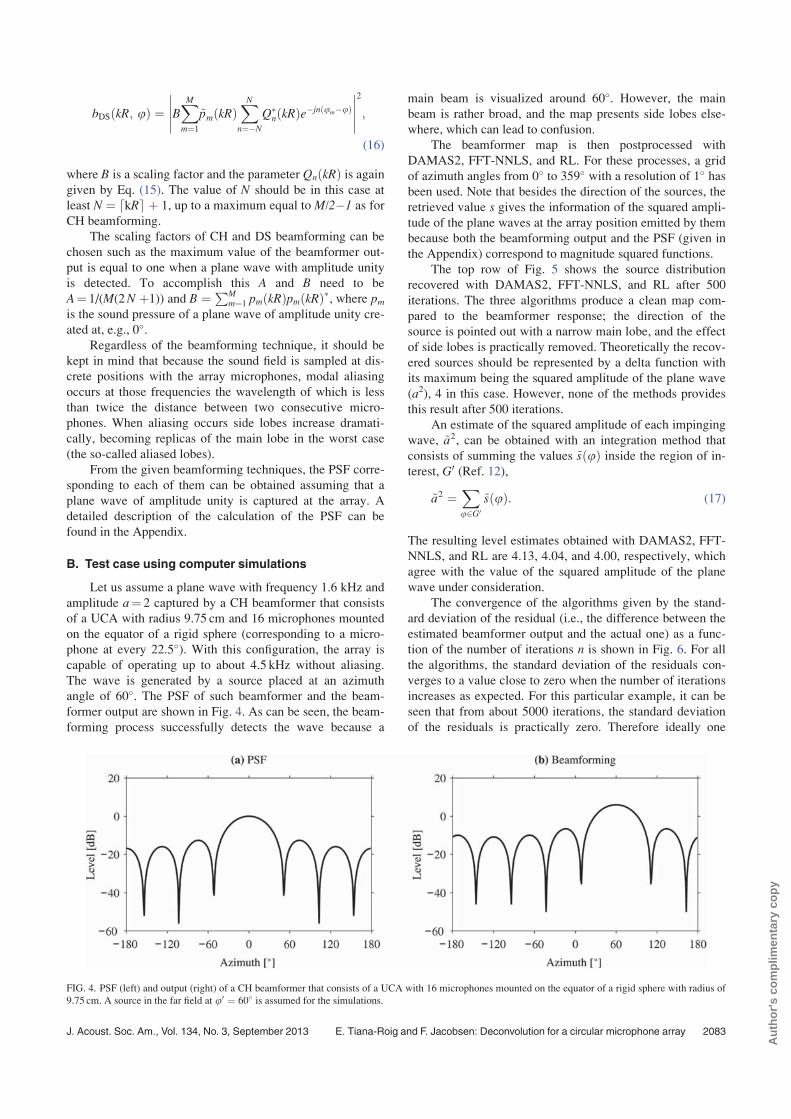
bDSðkR; uÞ ¼ BXMm¼1
~pmðkRÞXNn¼�N
Q�nðkRÞe�jnðum�uÞ
����������2
;
(16)
where B is a scaling factor and the parameter QnðkRÞ is againgiven by Eq. (15). The value of N should be in this case at
least N ¼ dkRe þ 1, up to a maximum equal to M/2�1 as for
CH beamforming.
The scaling factors of CH and DS beamforming can be
chosen such as the maximum value of the beamformer out-
put is equal to one when a plane wave with amplitude unity
is detected. To accomplish this A and B need to be
A¼ 1/(M(2N þ1)) and B ¼PMm¼1 pmðkRÞpmðkRÞ�, where pm
is the sound pressure of a plane wave of amplitude unity cre-
ated at, e.g., 0�.Regardless of the beamforming technique, it should be
kept in mind that because the sound field is sampled at dis-
crete positions with the array microphones, modal aliasing
occurs at those frequencies the wavelength of which is less
than twice the distance between two consecutive micro-
phones. When aliasing occurs side lobes increase dramati-
cally, becoming replicas of the main lobe in the worst case
(the so-called aliased lobes).
From the given beamforming techniques, the PSF corre-
sponding to each of them can be obtained assuming that a
plane wave of amplitude unity is captured at the array. A
detailed description of the calculation of the PSF can be
found in the Appendix.
B. Test case using computer simulations
Let us assume a plane wave with frequency 1.6 kHz and
amplitude a¼ 2 captured by a CH beamformer that consists
of a UCA with radius 9.75 cm and 16 microphones mounted
on the equator of a rigid sphere (corresponding to a micro-
phone at every 22.5�). With this configuration, the array is
capable of operating up to about 4.5 kHz without aliasing.
The wave is generated by a source placed at an azimuth
angle of 60�. The PSF of such beamformer and the beam-
former output are shown in Fig. 4. As can be seen, the beam-
forming process successfully detects the wave because a
main beam is visualized around 60�. However, the main
beam is rather broad, and the map presents side lobes else-
where, which can lead to confusion.
The beamformer map is then postprocessed with
DAMAS2, FFT-NNLS, and RL. For these processes, a grid
of azimuth angles from 0� to 359� with a resolution of 1� hasbeen used. Note that besides the direction of the sources, the
retrieved value s gives the information of the squared ampli-
tude of the plane waves at the array position emitted by them
because both the beamforming output and the PSF (given in
the Appendix) correspond to magnitude squared functions.
The top row of Fig. 5 shows the source distribution
recovered with DAMAS2, FFT-NNLS, and RL after 500
iterations. The three algorithms produce a clean map com-
pared to the beamformer response; the direction of the
source is pointed out with a narrow main lobe, and the effect
of side lobes is practically removed. Theoretically the recov-
ered sources should be represented by a delta function with
its maximum being the squared amplitude of the plane wave
(a2), 4 in this case. However, none of the methods provides
this result after 500 iterations.
An estimate of the squared amplitude of each impinging
wave, ~a2, can be obtained with an integration method that
consists of summing the values ~sðuÞ inside the region of in-
terest, G0 (Ref. 12),
~a2 ¼Xu2G0
~sðuÞ: (17)
The resulting level estimates obtained with DAMAS2, FFT-
NNLS, and RL are 4.13, 4.04, and 4.00, respectively, which
agree with the value of the squared amplitude of the plane
wave under consideration.
The convergence of the algorithms given by the stand-
ard deviation of the residual (i.e., the difference between the
estimated beamformer output and the actual one) as a func-
tion of the number of iterations n is shown in Fig. 6. For all
the algorithms, the standard deviation of the residuals con-
verges to a value close to zero when the number of iterations
increases as expected. For this particular example, it can be
seen that from about 5000 iterations, the standard deviation
of the residuals is practically zero. Therefore ideally one
FIG. 4. PSF (left) and output (right) of a CH beamformer that consists of a UCA with 16 microphones mounted on the equator of a rigid sphere with radius of
9.75 cm. A source in the far field at u0 ¼ 60� is assumed for the simulations.
J. Acoust. Soc. Am., Vol. 134, No. 3, September 2013 E. Tiana-Roig and F. Jacobsen: Deconvolution for a circular microphone array 2083
Aut
hor's
com
plim
enta
ry c
opy

would expect a recovered source distribution represented by
a delta function with a level of 4 at 60�. However, even after
1� 106 iterations, the retrieved source distribution with
DAMAS2 and FFT-NNLS differs from a delta function as
can be seen in the bottom row of Fig. 5. In the case of RL,
the result is much closer to the ideal response, but a close-up
of the figure reveals that there is still some spreading (the
peak is not exactly 4 and the neighboring values are not
zero). This means that more iterations are needed to get a
response as close as possible to the ideal response.
The deconvolution processes are particularly useful
when more than one source are present in the sound field
because they make it possible to locate the different sources
even when they are not visible in the beamformer output.
Let us consider that besides the source at 60� responsible forthe previous plane wave with frequency 1.6 kHz, there is
another source at 90� that creates a plane wave with unity
amplitude at the same frequency. The two sources are inco-
herent. The beamformer map obtained with CH beamform-
ing is shown in Fig. 7. As can be seen, the beamforming map
reveals only a source located at about 60� (the maximum is
actually at 63�). Although the main beam presents an asym-
metric shape that can indicate that there is another source
present, it is not possible to state that this is placed at 90� asassumed.
After applying deconvolution the maps shown in Fig. 8
are achieved with 5000 iterations. The three methods reveal
FIG. 5. Maps retrieved with DAMAS2 (left column), FFT-NNLS (middle column), and RL (right column) after 500 iterations (top row), and after 1� 106 iter-
ations (bottom row). A source in the far field at u0 ¼ 60� is considered. CH beamforming is used prior to the deconvolution algorithms.
FIG. 6. Standard deviation of the residual as a function of the number of
iterations n, for DAMAS2, FFT-NNLS, and RL.
FIG. 7. Map obtained with CH beamforming. Two plane waves are present
in the sound field, one with amplitude 2 created at 60� and another one with
amplitude 1 created at 90�.
2084 J. Acoust. Soc. Am., Vol. 134, No. 3, September 2013 E. Tiana-Roig and F. Jacobsen: Deconvolution for a circular microphone array
Aut
hor's
com
plim
enta
ry c
opy

two sources, the strongest being located at 60� as expected.
However, the other source is not exactly located at 90� but
close to it: at 94� with DAMAS2, at 92� with FFT-NNLS,
and at 91� with RL. The estimates of the squared amplitude
of the sources are very close to the expected level of the two
waves (22 and 12); 4.2 and 0.8 with DAMAS2, 4.1 and 0.9
with FFT-NNLS, and 4.0 and 0.9 with RL. As in the case of
having only one source, it can be shown that with the
increase of the number of iterations the maps become
clearer, and moreover the source with less energy is located
at an azimuth angle that tends to the actual value.
Although not shown similar results are obtained with
DS beamforming.
C. Simulated and experimental data results
The deconvolution methods DAMAS2, FFT-NNLS, and
RL have been tested experimentally and compared to com-
puter simulations. For this purpose, measurements with the
UCA shown in Fig. 3 were carried out in an anechoic room
with a volume of about 1000 m3. The array consisted of 16
1/4 in. microphones, Br€uel and Kjær (B&K) type 4958,
mounted on the equator of a rigid sphere with a radius of
9.75 cm. The array and the source, a loudspeaker, were con-
trolled by a B&K PULSE analyzer. The loudspeaker was
placed at 4m from the array center but at the very same
height at an azimuth angle of 180�. It was driven by a signal
from the generator, pseudorandom noise of 1 s of period,
6.4 kHz of bandwidth, and 1Hz of resolution. The signal had
a duration of 5 s. The microphone signals were recorded
with the analyzer, and after averaging for each channel, they
were postprocessed with CH beamforming and DS beam-
forming in the frequency range from 50 Hz to 5.5 kHz.
These procedures scanned directions from 0� to 359� with a
resolution of 1�. Subsequently the obtained beamforming
maps were processed with DAMAS2, FFT-NNLS, and RL,
using 500 iterations.
1. Sound source localization
To analyze the performance of the deconvolution meth-
ods in terms of localization of sound sources, the beamform-
ing maps prior to the deconvolution algorithms were
normalized for simplicity.
The left side of Fig. 9 shows the normalized output
obtained with CH beamforming and the source distribution
maps obtained with deconvolution as a function of fre-
quency. The predictions made with computer simulations are
also depicted on the right side of the figure.
To account for the background noise present in the
measurements, the simulations were carried out with a sig-
nal-to-noise ratio (SNR) of 30 dB at the input of each micro-
phone due to uniformly distributed noise.
At first sight, it can be seen that measurements and simu-
lations yield very similar results. The beamformer procedure
(top row) reveals the direction of the main source at 180� in
all the frequency range, but the main lobe is rather broad, spe-
cially at low frequencies, and side lobes appear along the map.
However, the map is satisfactorily improved after applying
DAMAS2 (second row), FFT-NNLS (third row), and RL (bot-
tom row) because the main lobe becomes more directive and
side lobes are reduced significantly. Interestingly, these proce-
dures can still visualize the direction of the source clearly at
those frequencies where aliasing in the beamforming map
occurs, this is, above 4.5 kHz approximately. This effect could
be important for those applications dealing with broadband
sources. However, it has been observed that the retrieved map
is free of aliasing just when a single source is present.
The results obtained with DS beamforming as well as
the recovered maps after deconvolution are shown in
Fig. 10. In this case, there is also a very good agreement
between measurements and simulations. Similar to the
results obtained with CH beamforming, the deconvolution
algorithms yield an improved version of the beamforming
map. Furthermore, they are capable of unveiling the direc-
tion of the source at very low frequencies where the DS
beamformer is omnidirectional.
For both techniques, it can be seen that in the case under
analysis 500 iterations are sufficient to demonstrate a clear
improvement of the maps after deconvolution. However, the
width of the main beam is not constant after the deconvolu-
tion processes; it becomes narrower with increasing fre-
quency. This implies that to obtain better results at the lower
frequencies, the deconvolution algorithms should include
more iterations.
Although a comparison of the three techniques could be
done at this point, this is out of the scope of the present study
FIG. 8. Maps retrieved with DAMAS2, FFT-NNLS, and RL after 5000 iterations. Two sources in the far field at 60� and 90� are considered. CH beamforming
is used prior to the deconvolution algorithms.
J. Acoust. Soc. Am., Vol. 134, No. 3, September 2013 E. Tiana-Roig and F. Jacobsen: Deconvolution for a circular microphone array 2085
Aut
hor's
com
plim
enta
ry c
opy

because it has been observed that their performance depends
strongly on the case under analysis.
2. Estimated sound pressure level
The sound pressure level of the impinging waves at the
array can be estimated after deconvolution by means of the
estimated squared amplitude, see Eq. (17). As mentioned in
Sec. II, the level of the sources cannot be estimated because
these are assumed to be in the far field of the array, and
therefore the wave fronts at the array position are practically
planar.
The estimated sound pressure level obtained after
deconvolution is similar to the sound pressure level captured
FIG. 9. (Color online) Normalized output obtained with CH beamforming (top row) and resulting maps after applying DAMAS2 (second row), FFT-NNLS
(third row), and RL (bottom row). The left column shows experimental results and the right column computer simulations.
2086 J. Acoust. Soc. Am., Vol. 134, No. 3, September 2013 E. Tiana-Roig and F. Jacobsen: Deconvolution for a circular microphone array
Aut
hor's
com
plim
enta
ry c
opy

by the array microphones. To show this, in Fig. 11 the
sound pressure level averaged across the array microphone
signals is plotted together with the estimated sound pressure
level retrieved with DAMAS2 when CH and DS
beamforming are used prior to the deconvolution process.
Note that for this analysis, the beamforming maps were not
normalized, so that the recovered sound pressure level is
comparable to the averaged sound pressure level captured by
microphones.
The agreement between the estimated sound pressure
level obtained after deconvolution and the averaged sound
pressure level of the microphone signals is particularly good
at lower frequencies. In fact, the curves are totally over-
lapped at these frequencies in the case of DS beamforming
FIG. 10. (Color online) Normalized output obtained with DS beamforming (top row) and resulting maps after applying DAMAS2 (second row), FFT-NNLS
(third row), and RL (bottom row). The left column shows experimental results and the right column computer simulations.
J. Acoust. Soc. Am., Vol. 134, No. 3, September 2013 E. Tiana-Roig and F. Jacobsen: Deconvolution for a circular microphone array 2087
Aut
hor's
com
plim
enta
ry c
opy

prior to the deconvolution process, probably due to the
robustness of this technique. With increasing frequency, the
retrieved level with deconvolution becomes lower than the
mean level of the microphones. The difference between low
and high frequencies is given by the fact that at low frequen-
cies, the rigid sphere does not affect the sound field, whereas
at high frequencies, it acts as a scatterer. The averaged pres-
sure at the microphones is amplified due to the scattering effect
at these frequencies. However, with deconvolution, the effect
of the scatterer is removed because this is accounted for in the
beamforming algorithms given in Eqs. (14) and (16).
Although not shown, very similar results were obtained
with FFT-NNLS and RL.
V. CONCLUSIONS
A UCA can be used for scanning the sound field over
360� to detect sound sources located in the array plane. By
means of beamforming procedures, the direction of the exist-
ing incoherent sound sources can be found, but these proce-
dures give rise to a blurred map. An investigation for
improving the visualization of the beamforming map has
been carried out by applying deconvolution procedures,
which are capable of recovering the location of the actual
sources with improved precision. The resulting maps present
better resolution and are practically free from effects of side
lobes. The deconvolution methods methods initially sug-
gested for planar sparse arrays have been adapted to the cir-
cular geometry, which has the advantage that beamforming
maps can be deblurred very efficiently with those deconvolu-
tion methods based on spectral procedures, namely,
DAMAS2, FFT-NNLS, and RL. The performance of these
methods has been examined for two beamforming techni-
ques, DS and CH beamforming, with computer simulations
and experimental results. For the three deconvolution meth-
ods, the resulting maps are improved by applying the decon-
volution algorithms in comparison with the conventional
beamforming maps.
APPENDIX: CALCULATION OF THE BEAMFORMER’SPSF
Consider a plane wave of amplitude a created by a sourcein the far field of a UCA, aejk�r
0. When the array is mounted
on a sphere, the pressure captured at the surface of the sphere,
at a point with spherical coordinates ½R; h; u, is23,24
pðkR; h; u; h0; u0Þ
¼ 4paX1q¼0
bqðkRÞXqv¼�q
Yvqðh; uÞYv
qðh0; u0Þ�; (A1)
where
bqðkRÞ ¼ ð�jÞq jqðkRÞ �j0qðkRÞh0qðkRÞ
hqðkRÞ !
; (A2)
Yvqðh; uÞ
ffiffiffiffiffiffiffiffiffiffiffiffiffiffiffiffiffiffiffiffiffiffiffiffiffiffiffiffiffiffiffiffiffið2qþ 1Þ
4pðq� vÞ!ðqþ vÞ!
sPvqðcos hÞejvu: (A3)
Note that in Eq. (A1), the temporal term e�jxt is omitted;
and the angles of the position of the source ½h0; u0 are used
instead of the angles of the incident wave ½hk; uk; thesebeing related by h0 ¼ p� hk and u0 ¼ uk þ p because the
unit vector of the incident wave k is opposite to the unit vec-
tor of the position of the source r0, k ¼ �r0.At the position of each microphone, ½R; p=2; um, the
pressure is
~pmðkRÞ ¼ pðkR; p=2; um; h0;u0Þ: (A4)
In the present study, the PSF is defined as the beam-
former response to a plane wave of unit amplitude created
by a source placed in the far field of the array, but at its very
same plane, i.e., at an inclination angle h0 ¼ p/2 and azimuth
angle u0. The PSF is then obtained when the expression
given in Eq. (A4) for a plane wave with amplitude a¼ 1 is
inserted into the beamformers output given in Eqs. (14) and
(16) for CH and DS beamforming, respectively. It should be
emphasized that the PSF considered in the deconvolution
methods presented in Sec. III requires that the source used
for its calculation is placed at an angle u0 ¼ 0; see Eq. (5).
With these considerations the expressions of the PSF for CH
and DS beamforming result in
FIG. 11. Averaged sound pressure level captured by the array microphones
and estimated sound pressure level obtained with DAMAS2. Maps with CH
beamforming (top) and DS beamforming (bottom) are obtained prior to
deconvolution.
2088 J. Acoust. Soc. Am., Vol. 134, No. 3, September 2013 E. Tiana-Roig and F. Jacobsen: Deconvolution for a circular microphone array
Aut
hor's
com
plim
enta
ry c
opy
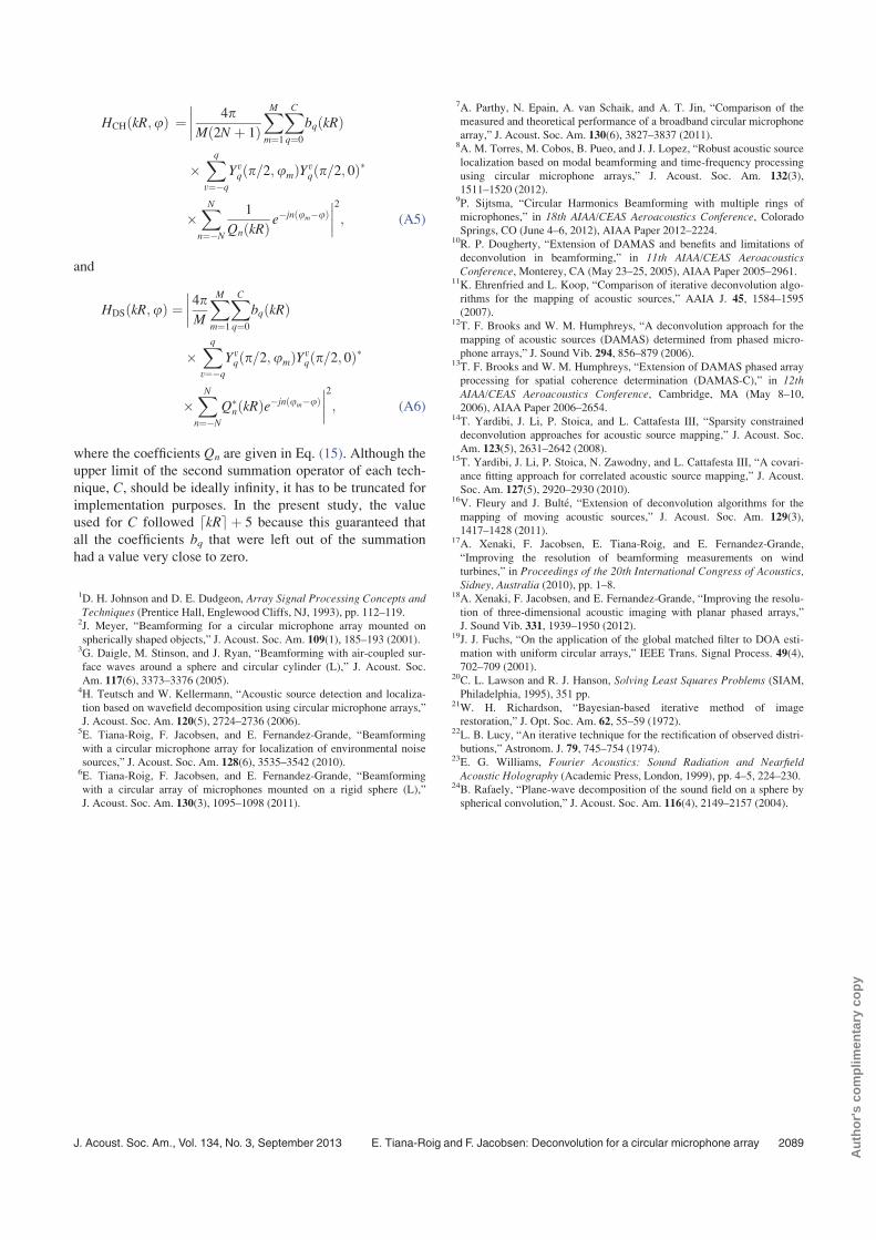
HCHðkR;uÞ ¼���� 4pMð2N þ 1Þ
XMm¼1
XCq¼0
bqðkRÞ
�Xqv¼�q
Yvqðp=2;umÞYv
qðp=2; 0Þ�
�XNn¼�N
1
QnðkRÞ e�jnðum�uÞ
����2
; (A5)
and
HDSðkR;uÞ ¼���� 4pM
XMm¼1
XCq¼0
bqðkRÞ
�Xqv¼�q
Yvqðp=2;umÞYv
qðp=2; 0Þ�
�XNn¼�N
Q�nðkRÞe�jnðum�uÞ
����2
; (A6)
where the coefficients Qn are given in Eq. (15). Although the
upper limit of the second summation operator of each tech-
nique, C, should be ideally infinity, it has to be truncated for
implementation purposes. In the present study, the value
used for C followed dkRe þ 5 because this guaranteed that
all the coefficients bq that were left out of the summation
had a value very close to zero.
1D. H. Johnson and D. E. Dudgeon, Array Signal Processing Concepts andTechniques (Prentice Hall, Englewood Cliffs, NJ, 1993), pp. 112–119.
2J. Meyer, “Beamforming for a circular microphone array mounted on
spherically shaped objects,” J. Acoust. Soc. Am. 109(1), 185–193 (2001).3G. Daigle, M. Stinson, and J. Ryan, “Beamforming with air-coupled sur-
face waves around a sphere and circular cylinder (L),” J. Acoust. Soc.
Am. 117(6), 3373–3376 (2005).4H. Teutsch and W. Kellermann, “Acoustic source detection and localiza-
tion based on wavefield decomposition using circular microphone arrays,”
J. Acoust. Soc. Am. 120(5), 2724–2736 (2006).5E. Tiana-Roig, F. Jacobsen, and E. Fernandez-Grande, “Beamforming
with a circular microphone array for localization of environmental noise
sources,” J. Acoust. Soc. Am. 128(6), 3535–3542 (2010).6E. Tiana-Roig, F. Jacobsen, and E. Fernandez-Grande, “Beamforming
with a circular array of microphones mounted on a rigid sphere (L),”
J. Acoust. Soc. Am. 130(3), 1095–1098 (2011).
7A. Parthy, N. Epain, A. van Schaik, and A. T. Jin, “Comparison of the
measured and theoretical performance of a broadband circular microphone
array,” J. Acoust. Soc. Am. 130(6), 3827–3837 (2011).8A. M. Torres, M. Cobos, B. Pueo, and J. J. Lopez, “Robust acoustic source
localization based on modal beamforming and time-frequency processing
using circular microphone arrays,” J. Acoust. Soc. Am. 132(3),1511–1520 (2012).
9P. Sijtsma, “Circular Harmonics Beamforming with multiple rings of
microphones,” in 18th AIAA/CEAS Aeroacoustics Conference, ColoradoSprings, CO (June 4–6, 2012), AIAA Paper 2012–2224.
10R. P. Dougherty, “Extension of DAMAS and benefits and limitations of
deconvolution in beamforming,” in 11th AIAA/CEAS AeroacousticsConference, Monterey, CA (May 23–25, 2005), AIAA Paper 2005–2961.
11K. Ehrenfried and L. Koop, “Comparison of iterative deconvolution algo-
rithms for the mapping of acoustic sources,” AAIA J. 45, 1584–1595(2007).
12T. F. Brooks and W. M. Humphreys, “A deconvolution approach for the
mapping of acoustic sources (DAMAS) determined from phased micro-
phone arrays,” J. Sound Vib. 294, 856–879 (2006).13T. F. Brooks and W. M. Humphreys, “Extension of DAMAS phased array
processing for spatial coherence determination (DAMAS-C),” in 12thAIAA/CEAS Aeroacoustics Conference, Cambridge, MA (May 8–10,
2006), AIAA Paper 2006–2654.14T. Yardibi, J. Li, P. Stoica, and L. Cattafesta III, “Sparsity constrained
deconvolution approaches for acoustic source mapping,” J. Acoust. Soc.
Am. 123(5), 2631–2642 (2008).15T. Yardibi, J. Li, P. Stoica, N. Zawodny, and L. Cattafesta III, “A covari-
ance fitting approach for correlated acoustic source mapping,” J. Acoust.
Soc. Am. 127(5), 2920–2930 (2010).16V. Fleury and J. Bult�e, “Extension of deconvolution algorithms for the
mapping of moving acoustic sources,” J. Acoust. Soc. Am. 129(3),1417–1428 (2011).
17A. Xenaki, F. Jacobsen, E. Tiana-Roig, and E. Fernandez-Grande,
“Improving the resolution of beamforming measurements on wind
turbines,” in Proceedings of the 20th International Congress of Acoustics,Sidney, Australia (2010), pp. 1–8.
18A. Xenaki, F. Jacobsen, and E. Fernandez-Grande, “Improving the resolu-
tion of three-dimensional acoustic imaging with planar phased arrays,”
J. Sound Vib. 331, 1939–1950 (2012).19J. J. Fuchs, “On the application of the global matched filter to DOA esti-
mation with uniform circular arrays,” IEEE Trans. Signal Process. 49(4),702–709 (2001).
20C. L. Lawson and R. J. Hanson, Solving Least Squares Problems (SIAM,
Philadelphia, 1995), 351 pp.21W. H. Richardson, “Bayesian-based iterative method of image
restoration,” J. Opt. Soc. Am. 62, 55–59 (1972).22L. B. Lucy, “An iterative technique for the rectification of observed distri-
butions,” Astronom. J. 79, 745–754 (1974).23E. G. Williams, Fourier Acoustics: Sound Radiation and NearfieldAcoustic Holography (Academic Press, London, 1999), pp. 4–5, 224–230.
24B. Rafaely, “Plane-wave decomposition of the sound field on a sphere by
spherical convolution,” J. Acoust. Soc. Am. 116(4), 2149–2157 (2004).
J. Acoust. Soc. Am., Vol. 134, No. 3, September 2013 E. Tiana-Roig and F. Jacobsen: Deconvolution for a circular microphone array 2089
Aut
hor's
com
plim
enta
ry c
opy

Paper D


Towards an enhanced performance of uniform circular arrays atlow frequencies
Elisabet Tiana-Roig 1, Antoni Torras-Rosell 2, Efren Fernandez-Grande 3, Cheol-Ho Jeong 4, and
Finn T. Agerkvist 5
1, 3, 4, 5Acoustic Technology, Dep. Electrical Engineering,
Technical University of Denmark, Ørsteds Plads 352, 2800 Kgs. Lyngby, Denmark
2DFM, Danish National Metrology Institute,
Matematiktorvet 307, 2800 Kgs. Lyngby, Denmark
ABSTRACTBeamforming using uniform circular arrays of microphones can be used, e.g., for localization of environmen-tal noise sources and for conferencing. The performance depends strongly on the characteristics of the array,for instance the number of transducers, the radius and whether the microphones are mounted on a scatterersuch as a rigid cylinder or a sphere. The beamforming output improves with increasing frequency, up to acertain frequency where spatial aliasing occurs. At low frequencies the performance is limited by the radiusof the array; in other words, given a certain number of microphones, an array with a larger radius will performbetter than a smaller array. The aim of this study is to improve the performance of the array at low frequencieswithout modifying its physical characteristics. This is done by predicting the sound pressure at a virtual andlarger concentric array. The propagation of the acoustic information captured by the microphones to the vir-tual array is based on acoustic holography. The predicted pressure is then used as input of the beamformingprocedure. The combination of holography and beamforming for enhancing the beamforming output at lowfrequencies is examined with computer simulations and experimental results.Keywords: Uniform circular array, Beamforming, Holography
1. INTRODUCTIONBeamforming based on a uniform circular array of microphones (UCA) is a well-known method to
localize sound sources around the array from 0 to 360◦. In the present paper, the main concern is the im-provement of the performance at low frequencies. In the recent years, various strategies have been suggested
1 [email protected] [email protected] [email protected] [email protected] [email protected]

in this matter, such as the design of beamforming techniques other than delay-and-sum. For instance, circu-lar harmonics beamforming is a clear example of how a beamforming technique can be designed to suit aparticular geometry, in this case, the circular geometry. This technique is based on the decomposition of thesound field in a series of coefficients by means of a Fourier series.1 With this technique most of the frequencyrange is improved. Another possibility is to flush-mount the microphones on a rigid baffle, such as a rigidsphere or a spherical cylinder. The effect of the scatterer has proved to be beneficial compared to the casewhere the array microphones are suspended in the free space.2–4 Yet another alternative is the use of de-convolution methods, which clean the beamforming map by means of iterative algorithms to finally recoverthe distribution of the sources present in the sound field. These methods are very effective, but require highcomputational effort, in particular at low frequencies. Methods such as the Deconvolution Approach for theMapping of Acoustic Sources 2 (DAMAS2), the Fourier-based Non-Negative Least Squares (FFT-NNLS)and the Richardson-Lucy (RL) have already been adapted to the circular geometry.5,6
In all cases the performance improves with increasing frequency, up to a frequency where spatial alias-ing occurs. The poor performance at the lowest frequencies is especially of concern with delay-and-sumbecause this presents an omnidirectional pattern, and therefore sources in this frequency range cannot belocalized. Although the use of a scatterer improves its performance, it does not completely eliminate thisproblem. With deconvolution methods the low frequency problems can be resolved, even with beamform-ing patterns obtained originally with delay-and-sum. However if the same resolution is to be achieved inthe entire frequency range, the lower the frequency the more the iterations needed. Or in other words, thedeconvolution methods are less efficient at low frequencies.
In this article we suggest a simple method to improve the performance of UCAs at low frequencies,which does not imply the design of new beamforming techniques or a modification of the geometry of thearray. The basic idea is that for a specific number of microphones, a UCA with a larger radius will performbetter at low frequencies than an array with a smaller radius, because the distance between the microphoneswill be larger, and the wavelengths corresponding to the low frequencies will be better captured. Inspired bythis concept, one could measure the sound field with a UCA, and by means of acoustic holography predictthe sound pressure at a larger and virtual radius. The estimated pressure could be then used as input to thebeamforming algorithm. A sketch of the procedure can be seen in Fig. 1.
virtual array
physical array
acoustical
holography beamforming
beamforming map
Fig. 1 – Sketch of the procedure for the calculation of the beamforming map. The pressure captured by aUCA is used for the prediction of the pressure at a larger and virtual array by means of acoustical
holography. The predicted pressure is used as input of the beamforming procedure.
The combination of holography and beamforming for the improvement of the performance at low fre-quencies is the subject of study in the present work, and this is examined by means of computer simulationsand experiments.
2. BACKGROUND THEORY2.1. Acoustic Holography
Acoustic holography is a sound visualization technique that makes it possible to reconstruct the soundfield over a three-dimensional space based on a two dimensional measurement. Often, the measurement isperformed close to the source, as in near-field acoustic holography (NAH) to capture the evanescent wavesfor an enhanced spatial resolution.7,8 However, in the present study we are concerned with the reconstructionof the sound field in the far field, prior to the beamforming processing.

In acoustic holography, the measured sound field is typically expanded into a series of basis functionsfrom which the entire acoustic field can be reconstructed. In this paper we focus on a circular space, makinguse of the fact that the sound field can be predicted on different radii by means of the Bessel functionsthat account for the propagation in the radial direction. This approach is in a sense analogous to the onecommonly used for NAH in spherical coordinates,9–11 but in this case the radial functions are conventionalBessel functions, and the angular dependency is reduced to the azimuth only, as it follows from a circularharmonic expansion. It is worth noting that the inverse holographic reconstruction, i.e., when propagatingtowards the source, is an ill-posed problem that requires regularization. It has been shown that in the case ofspherical NAH, truncation is an appropriate regularization procedure.12 Similarly, truncation is adequate forthe circular geometry.
Let us consider that a plane wave that travels perpendicularly to the z-axis (i.e., the wavefronts areparallel to the z-axis) is captured by a UCA of radius R placed at the xy-plane, at z = 0. The sound pressureat the array can be represented in terms of solutions of the Helmholtz equation in a cylindrical coordinatesystem with origin at the center of the UCA. After applying the boundary conditions (basically that the soundfield at the origin must be finite), the pressure can be expressed as7
p(kr, ϕ) =∞∑
n=−∞AnJn(kr)e
jnϕ, (1)
where k is the wavenumber and An is the coefficient of the n’th term. As can be seen the angular dependencyof the pressure is given by the circular harmonics ejnϕ, whereas the radial dependency is given by the Besselfunctions Jn. Note that the time dependency e−jωt is omitted. The previous expression can be ideally usedto determine a particular sound field at any point by means of acoustic holography. For this purpose we needto determine the values of the coefficients An. The pressure at the UCA, at r = R is
p(kR, ϕ) =∞∑
n=−∞AnJn(kR)ejnϕ. (2)
Making use of the orthogonality of the circular harmonics,
1
2π
∫ 2π
0
ejnϕe−jmϕdϕ = δmn, (3)
the coefficients An can be retrieved by multiplying each side of Eq. (2) by a complex conjugated circularharmonic and integrating over the entire circle, from 0 to 2π. The resulting expression follows
An =12π
∫ 2π
0p(kR, ϕ)e−jnϕdϕ
Jn(kR). (4)
This expression implies a continuous integral of the sound pressure. However the pressure is known atdiscrete positions, because the sound field is sampled with M microphones. Therefore, the integral must beapproximated by means of a finite summation:∫ 2π
0
p(kR, ϕ)e−jnϕdϕ ⇒M∑i=1
αip(kR, ϕi)e−jnϕi , (5)
where the coefficients αi must equal 2π/M to keep the orthogonality properties of the circular harmonicsgiven in Eq. (3) in discrete notation. Finally the coefficients An are calculated as
An =1M
∑Mi=1 p(kR, ϕi)e
−jnϕi
Jn(kR). (6)
By inserting this expression into Eq. (1), the sound pressure can be, in principle, predicted anywhere. Asmentioned earlier, regularization is needed in practice. This is done by truncating the limits of the summationpresented in Eq. (2) to certain values −N and N ,
p(kr, ϕ) =
N∑n=−N
AnJn(kr)ejnϕ. (7)
It can be shown that a reasonable value of N follows N = �kr�+ 1, where �·� is the ceiling function, up toa maximum value M/2− 1.
2.2. BeamformingBeamforming is a signal processing technique commonly used in acoustics to localize sound sources.
The beamforming technique used in the present study is the classical delay-and-sum beamforming, whichis a very simple, but robust, method. It is based on delaying the signals of each array microphone by acertain amount and adding them together, to reinforce the resulting signal. Depending on the delay applied tothe different microphones the array is steered to a particular direction.13 Expressed in the spatial frequencydomain the beamforming output follows
b(kR, ϕ) = AM∑
m=1
wip(kR, ϕm)p∗(kR, ϕm), (8)
where wm is the weighting coefficient of the m’th microphone, p(kR, ϕm) is the pressure measured at them’th microphone, and p∗(kR, ϕm) is the theoretical complex conjugated pressure due to a plane wave withorigin at ϕ. In the presence of a single source, when the beamformer is focused to the direction of the actualsource, the maximum output is achieved. Ideally the beamformer would present a peak at the direction of thesource and zeros elsewhere, but this is not the case due to the fact that the sound field is captured at discretepositions with the microphones. This implies that the beamforming map presents a main lobe around thedirection of the source and side lobes elsewhere.
In case of an unbaffled UCA, the theoretical pressure is simply the closed form for a plane wave, ejk·r,at the array microphones, so the beamformer output is
b(kR, ϕ) =1
M
M∑m=1
p(kR, ϕm)ejkR cos(ϕm−ϕ). (9)
Note that the weights wm have been set to 1 and A = 1/M , in order to have a maximum beamformer outputequal to one when a plane wave of amplitude unity is present.
Although the focus of the current study is the improvement of the performance at low frequencies, itshould be mentioned that the operation of a beamformer is limited at high frequencies when the Nyquistsampling criterion is not fulfilled, i.e., at those frequencies whose corresponding wavelengths are less thantwice the distance between two adjacent microphones. When aliasing occurs side lobes increase dramatically,becoming replicas of the main lobe in the worst case (the so-called aliased lobes).
2.3. Combining acoustic holography with beamformingThe aim of this study is to combine acoustic holography and beamforming to improve the beamforming
output at low frequencies. As shown in Fig. 1 the pressure is measured with a UCA of radius R and Mmicrophones placed at ϕi. By means of holography the pressure is predicted at a larger and virtual array ofradius Rv. In the present study the number of virtual microphones and their azimuth angles are the same as forthe actual array. In fact, by means of simulations it has been observed that the position of the microphones isnot that relevant as long as the distance between microphones remains constant. This makes sense since UCAsare practically shift-invariant, i.e., the beamforming pattern is the same regardless the focusing direction.14
The pressure predicted with acoustic holography, which follows from evaluating Eq. (1) at (Rv, ϕi), is
then used as input of the beamforming procedure. The coefficients An given in Eq. (6) are obtained withthe pressure measured with the actual array microphones. Then the beamforming algorithm follows frominserting Eqs. (6) and (7) into Eq. (9),
b(kRv, ϕ) =1
M2
M∑m=1
N∑n=−N
M∑i=1
p(kR, ϕi)Jn(kRv)
Jn(kR)ej(n(ϕm−ϕi)+kRv cos(ϕm−ϕ)), (10)
where N = �kRv�+ 1, up to a maximum value M/2− 1.
3. RESULTS AND DISCUSSION3.1. Computer simulations
The effect of combining beamforming and holography is analyzed in this section by means of computersimulations. A UCA like the one shown in Fig. 2 has been assumed. The array radius is R = 11.9 cm and ithas 12 microphones. The array used for the simulations coincides with the array used for the measurements

Fig. 2 – Prototype UCA of radius 11.9 cm and 12 microphones used for the measurements.
presented in the next section. Following from the Nyquist sampling theorem, this array will present spatialaliasing from ca. 2.8 kHz.
A plane wave generated at 180◦ is considered. The frequency range of interest is from 50 Hz to 2 kHz. Asignal-to-noise ratio (SNR) of 30 dB at each array microphone due to uniformly distributed noise is assumedfor the simulations to account for background noise.
Beamforming has been performed in the usual way with the pressure at the array microphones followingfrom Sec. 2.2. Besides this, by means of holography, the simulated pressure has been used to predict thepressure at a larger and virtual radius, twice the size of the actual array radius (2R) at the same azimuthangles. The predicted pressure at the virtual array has been used for the beamforming procedure as indicatedin Sec. 2.3. In parallel, beamforming has been performed in ideal conditions (in absence of noise) with aUCA of radius 2R and 12 microphones. Note that for this case, as well as for the case of the virtual array,aliasing is expected from about 1.4 kHz; i.e., the operating frequency range is half the range of the array ofradius R.
For ease of understanding the resulting normalized beamforming outputs for a single frequency, in thiscase 400 Hz, are shown in Fig. 3. It can be seen that in all cases a main lobe around 180◦ is present, which
Azimuth [◦]
Bea
mfo
rmin
gou
tput
[dB
]
UCA – Rvirtual UCA – 2RUCA – 2R (w/o noise)
0 60 120 180 240 300 360−60
−50
−40
−30
−20
−10
0
Fig. 3 – Normalized beamforming outputs at 400 Hz obtained with three UCAs with 12 microphones: a realarray of radius R = 11.9 cm, a virtual array of radius 2R and a real array of radius 2R.
indicates that there is a source in this direction, as expected. However the main lobe obtained with the arraywith radius R is very wide, which can lead to confusion, whereas the virtual array and the array with radius2R present a narrower main lobe, which makes the interpretation of the map clearer.
The maps obtained for all frequencies are shown in Fig. 4. Note that Fig. 3 corresponds to a vertical cut

of the beamforming maps at 400 Hz.
Fig. 4 – Normalized beamforming maps obtained with three UCAs with 12 microphones. (Top) mapobtained with an array of radius R = 11.9 cm, (middle) map obtained with a virtual array of radius2R by means of combining holography and beamforming, and (bottom) ideal map obtained with anarray of radius 2R. A source at 180◦ is assumed. For the small and the virtual array a SNR of 30
dB is accounted for.
In all the cases the maps are omnidirectional at the lowest frequencies. With increasing frequency thepatterns become more directive, unveiling a source at 180◦. For the virtual array and the array of radius 2Raliasing is observed at about 1.4 kHz as expected.
The virtual array is more directive at low frequencies compared to the actual array of radius R as ex-pected from the theory. In fact the virtual array is omnidirectional in a narrower frequency range (half therange of the actual array) and from the upper frequency limit of the omnidirectional range it becomes moreand more directive. Regarding the level of the side lobes, it can be seen that in both cases the levels aresimilar.
The performance of the virtual array is very similar to the ideal performance of the array of radius 2R, upto the Nyquist sampling frequency where differences are observed. This shows that the virtual array behavesin this range as a real array with the same radius. The most apparent difference is the vertical line at 1103 Hz,which shows that for that frequency the beamforming is rather omnidirectional. This is caused by the fact

that the Bessel function in the denominator of Eq. (10) is zero for n = 0 at that frequency.Alternatively to the beamforming maps, the performance of the array can be analyzed by means of two
measures: the resolution and the maximum side lobe level (MSL). The resolution is the −3 dB width of themain lobe, whereas the MSL is the difference between the highest secondary lobe and the main lobe. In bothcases, the smaller the values, the better. The resolution and the MSL are shown in Fig. 5.
Frequency [Hz]
Res
olut
ion
[o ]
100 10000
60
120
180
240
300
360
Frequency [Hz]
MSL
[dB
]
UCA – Rvirtual UCA – 2RUCA – 2R (w/o noise)
100 1000−60
−50
−40
−30
−20
−10
0
Fig. 5 – Resolution (left) and MSL (right) obtained with UCA of radius R = 11.9 cm and 12 microphones, avirtual UCA with radius 2R, and an ideal UCA of radius 2R. A plane wave created by a source at
180◦ is assumed. For the small array and the virtual array a SNR of 30 dB is considered.
These two measures confirm that the virtual array behaves like a real array with the same dimensions,especially in terms of resolution, up to the frequencies where sampling error occurs. However, in terms ofMSL the levels are slightly higher for the virtual array from about 800 Hz. The peak at 1103 Hz seen inboth the resolution and MSL with the virtual array corresponds to the singularity observed previously in thebeamforming map.
3.2. Experimental resultsMeasurements with the prototype array with radius 11.9 cm and 12 microphones shown in Fig. 2 were
carried out in an anechoic room of dimensions 12.1 m × 9.7 m × 8.5 m. The array microphones were 1/4 in.microphones Bruel & Kjær (B&K) Type 4935.
A picture of the set-up is shown in Fig. 6. The array and the source placed in the far-field of the arraywere controlled by a B&K PULSE analyzer. The loudspeaker was driven with a signal from the generator,pseudorandom noise of 1 s of period, 3.2 kHz of bandwidth, and 1 Hz of resolution. Each microphone signalwas recorded with the analyzer, and after Fourier transforming they were postprocessed with beamforming.The resulting map can be seen in the top panel of Fig. 7.
The data from the microphones were used to predict the pressure by means of acoustical holography ata virtual UCA with twice the radius of the array used for the measurements. With the predicted pressure usedas input of the beamforming algorithm, the normalized map shown in the bottom of Fig. 7 was obtained. Ascan be seen the beamforming maps are very similar to the maps obtained with simulations in the previoussection, although they appear slightly more blurry.
The resolution and the MSL for the actual and the virtual arrays can be seen in Fig. 8. These twomeasures resemble the curves obtained with simulations. In terms of the resolution, the major differences areobserved in the peak at 1103 Hz, which is more abrupt, and in the region where aliasing occurs, althoughthis region is not of interest. For the MSL it can be seen that the curves appear slightly shifted towards highfrequencies compared with the simulations, and that the MSL of the virtual array is a bit higher than expectedin the range between 800 Hz and 1 kHz.
In any case, the results prove that at the low frequencies the actual (and small) array benefits from usingholography to predict the pressure at a larger and virtual radius and combine it with beamforming.
4. FINAL REMARKS AND FUTURE WORKIn this article it has been shown that the performance of delay-and-sum beamforming improves at low
frequencies by combining acoustic holography with beamforming. The procedure is the following: the pres-sure captured by a UCA is used to predict the pressure at a virtual array with a larger radius by means of

Fig. 6 – Measurement set-up.
Fig. 7 – (Top) Normalized beamforming map obtained with a UCA with 12 microphones and radius 11.9cm. The pressure captured by the array microphones is used to predict the pressure at a virtual
UCA with twice the radius of the original array by means of acoustical holography. The predictedpressure is used to compute the normalized beamfroming map (bottom).

Frequency [Hz]
Res
olut
ion
[o ]
100 10000
60
120
180
240
300
360
Frequency [Hz]
MSL
[dB
]
UCA – Rvirtual UCA – 2R
100 1000−60
−50
−40
−30
−20
−10
0
Fig. 8 – Resolution (left) and MSL (right) obtained with UCA of radius R = 11.9 cm and 12 microphonesand a virtual UCA with radius 2R. A plane wave was created by a source at 180◦.
acoustical holography. The predicted pressure is then used as input to the delay-and-sum beamforming al-gorithm. The benefits of using a virtual array have been proven by means of simulations and experimentalresults.
The combination of holography and beamforming adds new features to UCAs without any additionalcost. Specifically the array gains more flexibility, for example at high frequencies the array measurementscould be used directly for the beamforming procedure in the usual way, whereas at low frequencies acousticholography could be used prior to beamforming to enhance the beamforming map at those frequencies.
There are still some questions that need to be examined further, e.g., the effect of using other beam-forming techniques different from delay-and-sum beamforming, the applicability of the method in noisierconditions, and how large the virtual array can be. In this sense virtual arrays with radius larger than twicethe radius of the actual array have been tested. The results, which are not included in the article, reveal thatboth resolution and MSL become worse than expected with increasing the radius. However this statementneeds additional investigation.
The idea presented in the present study can be applied to other UCAs mounted on a scatterer such as arigid cylinder, or to spherical arrays to map a three dimensional sound field.
ACKNOWLEDGMENTSThe authors are thankful to Finn Jacobsen who was involved in this study at an early stage.
REFERENCES[1] E. Tiana-Roig, F. Jacobsen, and E. Fernandez-Grande, “Beamforming with a circular microphone array
for localization of environmental noise sources”, J. Acoust. Soc. Am. 128(6), 3535–3542 (2010).
[2] G. Daigle, M. Stinson, and J. Ryan, “Beamforming with air-coupled surface waves around a sphere andcircular cylinder (L)”, J. Acoust. Soc. Am. 117(6), 3373–3376 (2005).
[3] H. Teutsch and W. Kellermann, “Acoustic source detection and localization based on wavefield decom-position using circular microphone arrays”, J. Acoust. Soc. Am. 120(5), 2724–2736 (2006).
[4] E. Tiana-Roig, F. Jacobsen, and E. Fernandez-Grande, “Beamforming with a circular array of micro-phones mounted on a rigid sphere (L)”, J. Acoust. Soc. Am. 130(3), 1095–1098 (2011).
[5] E. Tiana-Roig and F. Jacobsen, “Acoustical source mapping based on deconvolution approaches forcircular microphone arrays”, in Proceedings of Inter-noise 2011, Osaka, Japan (2011).
[6] E. Tiana-Roig and F. Jacobsen, “Deconvolution for the localization of d sources using a circular micro-phone array,”, J. Acoust. Soc. Am. (To be published).
[7] E. G. Williams, Fourier Acoustics: Sound radiation and near field acoustic holography (Academic,London) (1999).
[8] J. D. Maynard, E. G. Williams, and Y. Lee, “Nearfield acoustic holography : I . Theory of generalizedholography and the development of NAH”, J. Acoust. Soc. Am. 78(4), 1395–1413 (1985).

[9] E. G. Williams, N. Valdivia, and P. C. Herdic, “Volumetric acoustic vector intensity imager”, J. Acoust.Soc. Am. 120(4), 1887–1897 (2006).
[10] E. G. Williams and K. Takashima, “Vector intensity reconstructions in a volume surrounding a rigidspherical microphone array”, J. Acoust. Soc. Am. 127(2), 773–783 (2010).
[11] F. Jacobsen, G. M. Pescador, E. Fernandez-Grande, and J. Hald, “Near field acoustic holography withmicrophones on a rigid sphere (L)”, J. Acoust. Soc. Am. 129(6), 3461–3464 (2011).
[12] A. Granados, F. Jacobsen, and E. Fernandez-Grande, “Regularized reconstruction of sound fields witha spherical microphone array”, in ICA 2013 Montreal, Montreal, Canada (2013).
[13] D. Johnson and D. Dudgeon, Array Signal Processing Concepts and Techniques (Prentice Hall, Engle-wood Cliffs, New Jersey) (1993).
[14] J. Meyer, “Beamforming for a circular microphone array mounted on spherically shaped objects”, J.Acoust. Soc. Am. 109(1), 185–193 (2001).

Paper D


BeBeC-2014-03
ENHANCING THE BEAMFORMING MAP OF SPHERICALARRAYS AT LOW FREQUENCIES USING ACOUSTIC
HOLOGRAPHY
Elisabet Tiana-Roig1, Antoni Torras-Rosell2, Efren Fernandez-Grande1,Cheol-Ho Jeong1 and Finn T. Agerkvist1
1Acoustic Technology, Dep. Electrical Engineering, Technical University of Denmark
Ørsteds Plads 352, 2800 Kgs. Lyngby, Denmark2DFM, Danish National Metrology Institute
Matematiktorvet 307, 2800 Kgs. Lyngby, Denmark
ABSTRACT
Recent studies have shown that the localization of acoustic sources based on circular ar-
rays can be improved at low frequencies by combining beamforming with acoustic holog-
raphy. This paper extends this technique to the three dimensional case by making use of
spherical arrays. The pressure captured by a rigid spherical array under free-field condi-
tions is used to compute the expected pressure on a virtual and larger sphere by means of
acoustic holography. Beamforming is then applied with the pressure predicted at the virtual
array. Since the virtual array has a larger radius compared to the one of the physical array,
the low frequencies (the ones with larger wavelength) are better captured by the virtual
array, and therefore, the performance of the resulting beamforming system is expected to
improve at these frequencies. The proposed method is examined with simulations based on
delay-and-sum beamforming. In addition, the principle is validated with experiments.
1 INTRODUCTION
Spherical arrays of microphones have been of interest in the last decade, because of the abilityto measure in a three-dimensional sound field [1, 2]. Typically, these arrays are suitable forsound source localization using beamforming [3–6] and for sound recording in higher orderreproduction systems such as Ambisonics [7–9].
1

5th Berlin Beamforming Conference 2014 Tiana-Roig et al.
Several strategies to improve the performance of beamforming systems have been suggestedin the recent years. For example, it has been shown that arrays with flushed-mounted mi-crophones on a rigid sphere perform better compared to open (or transparent) spherical ar-rays [2, 10, 11]. Besides this, different beamforming techniques have been designed for thisgeometry [6]. Among them, phase-mode (or spherical harmonics) beamforming is of particularinterest, because it exploits the spherical geometry by decomposing the sound field in a seriesof spherical harmonics. Compared to the classical delay-and-sum beamforming, phase-modebeamforming presents a better directivity, at the expense of being more sensitive to noise [5].In fact, delay-and-sum beamforming is a very robust technique, but it performs poorly at lowfrequencies, being omnidirectional in the worse case.
Inspired by an article on uniform circular arrays presented recently in Ref. [12], the presentarticle examines the possibility of enhancing the localization of noise sources with sphericalarrays at low frequencies by combining spherical acoustic holography [13–15] and delay-and-sum beamforming. The idea behind this concept is that for a given number of transducers,an array with a larger radius will perform better at low frequencies than a smaller array [2].However, if one cannot change the geometry of the array, a simple solution to obtain a virtuallylarger array is illustrated in Fig. 1: the sound pressure is captured with a spherical array (rigid ortransparent), and by means of acoustic holography the pressure is predicted at a virtual sphericalarray with larger radius. Finally the pressure at this virtual array is used for the beamformingprocess. The theory presented in this work is supplemented with simulations and measurements.
virtual array
physical array
acousticalholography beamforming
Figure 1: Procedure to obtain the beamforming map: the pressure captured by a spherical arrayis used to predict the pressure at a larger and virtual array with acoustic holography,and from this beamforming is carried out.
2
5th Berlin Beamforming Conference 2014 Tiana-Roig et al.
2 ACOUSTIC HOLOGRAPHY AND BEAMFORMING WITH A SPHERICALARRAY
2.1 Acoustic holography
Acoustic holography with a spherical array of transducers is a sound visualization technique thatenables the reconstruction of a sound field over the three-dimensional space, based only on thesound pressure or particle velocity captured with the array. Acoustic holography measurementsare usually performed very close to the source and the reconstruction lies somewhere betweenthe measurement position and the source, as in near-field acoustic holography (NAH). However,in the present study, measurements in the far field of the sound source are of concern.
Let us consider a rigid spherical array with radius R centered at the origin of the coordinatesystem. The pressure at a point outside the array is given by the sum of the incident soundpressure and the scattered pressure due to the presence of the sphere,
p = pinc + psca. (1)
Given the spherical geometry, it makes sense to describe both pressures in terms of solutionsof the Helmholtz equation in spherical coordinates (r,θ ,ϕ) (θ being the inclination angle withrespect to the z−axis and ϕ being the azimuth). The incident pressure, which is the one thatwould be measured if the scatterer was not present, must be described by means of sphericalBessel functions, because these are finite (even at the origin) [15, 16],
pinc(kr,θ ,ϕ) =∞
∑n=0
n
∑m=−n
Amn jn(kr)Y mn (θ ,ϕ), (2)
where jn is the spherical Bessel function of order n, and the terms Y mn are the so-called spherical
harmonics,
Y mn (θ ,ϕ) =
√2n+1
4π(n−m)!
(n+m)!Pm
n (cosθ)e jmϕ , (3)
in which Pmn is the associated Legendre function. Note that the time dependence e− jωt is omit-
ted. The scattered pressure must be described as outgoing waves, represented in this case by thespherical Hankel functions of the first kind [17],
psca(kr,θ ,ϕ) =∞
∑n=0
n
∑m=−n
Bmnh(1)n (kr)Y mn (θ ,ϕ), (4)
where h(1)n is the Hankel function of the first kind and order n.The relationship between the coefficients Amn and Bmn is given by the fact that the total radial
velocity at the surface of the rigid sphere (r = R) is zero. From this condition it follows that
Bmn =−Amnj′n(kR)
h′(1)n (kR), (5)
3

5th Berlin Beamforming Conference 2014 Tiana-Roig et al.
where j′n and h′(1)n are the radial derivatives of jn and h(1)n . Therefore, the total pressure is
p(kr,θ ,ϕ) =∞
∑n=0
n
∑m=−n
Amn
(jn(kr)− j′n(kR)
h′(1)n (kR)h(1)n (kr)
)Y m
n (θ ,ϕ). (6)
Since the pressure at the array is known, the coefficients Amn can be retrieved by making use ofthe orthogonality relationship of the spherical harmonics,
∫ 2π
0
∫ π
0Y m
n (θ ,ϕ)Y μν (θ ,ϕ)∗ sinθdθdϕ = δnνδmμ , (7)
where δnν is the Kronecker delta function. Then, it can be shown that the coefficients Amn are
Amn =
∫ 2π0
∫ π0 p(kR,θ ,ϕ)Y m
n (θ ,ϕ)∗ sinθdθdϕ
jn(kR)− j′n(kR)
h′(1)n (kR)h(1)n (kR)
. (8)
To implement this equation in practice, the integrals must be substituted by discrete summa-tions, capable of fulfilling the discrete orthogonality relationship of the spherical harmonics,which has to be accounted for in the design of the array,
M
∑i=0
αiY mn (θi,ϕi)Y
μν (θi,ϕi)
∗ = δnνδmμ for ν ≤ Nhol, n ≤ Nhol, (9)
where i represents the ith microphone at position (R,θi,ϕi), M is the number of sensors, andαi is an associated integration weight factor that guarantees orthogonality up to a certain orderNhol . Using the discrete orthogonality, the expression for the expansion coefficients Amn resultsin [15]
Amn =∑M
i=1 αi p(kR,θi,ϕi)Y mn (θi,ϕi)
∗
jn(kR)− j′n(kR)
h′(1)n (kR)h(1)n (kR)
. (10)
This relationship assumes that the highest order of spherical harmonics included in the soundpressure is lower or equal to Nhol . This is a reasonable assumption as long as the value kR isabout Nhol . When this requirement is not met aliasing occurs in the coefficients.
The coefficients Amn can be used to compute the incident pressure and the scattered pressureseparately (see Eqs. (2) and (4)) and the total pressure (see Eq. (6)) at a point (r,θ ,ϕ).
2.2 Beamforming
Beamforming is a signal processing technique well used for localization of sound sources.There are several beamforming methods, but in the present study, delay-and-sum beamformingis chosen. Although this method is the oldest one, it is still widely used due to its robustness.It consists of delaying the signals of each array microphone by a certain amount and addingthem together, to reinforce the resulting signal. Depending on the delay applied to the differentmicrophones, the array is steered to a particular direction, whereas other directions are totallyor partially attenuated [18]. Since in the current study the array is mounted on a rigid sphere,
4
5th Berlin Beamforming Conference 2014 Tiana-Roig et al.
it is simpler to express the beamforming output in the spatial frequency domain, because thisallows us to compensate for the effect of the scatterer. In this domain the output is
b(kR,θ ,ϕ) = BM
∑i=1
wi p(kR,θi,ϕi)p(kR,θi,ϕi|θ ,ϕ)∗, (11)
where B is a scaling factor, wi is a weighting factor, p is the measured pressure at the ithmicrophone, while p corresponds to the theoretical pressure at the ith microphone due to asource in the far-field at (θ ,ϕ). It can be shown that the pressure at (R,θi,ϕi) due to a planewave created by a source at (θ ,ϕ) is [4]
p(R,θi,ϕi) =∞
∑n=0
n
∑m=−n
Qn(kR)Y mn (θi,ϕi)Y m
n (θ ,ϕ)∗, (12)
where Qn is
Qn(kR) = 4π(− j)n
(jn(kR)− j′n(kR)
h′(1)n (kR)h(1)n (kR)
). (13)
Making use of this expression the output of the delay-and-sum beamformer is
b(kR,θ ,ϕ) = BM
∑i=1
wi p(kR,θi,ϕi)N
∑n=0
(Qn(kR)
n
∑m=−n
Y mn (θi,ϕi)Y m
n (θ ,ϕ)∗)∗
. (14)
Note that the second summation has to be truncated at N for the real implementation. A reason-able value is N ≈ kR+1. By making use of the addition theorem [19] that states that
Pn(cosψq) =4π
2n+1
n
∑m=−n
Y mn (θ ,ϕ)Y m
n (θq,ϕq)∗, (15)
wherecos(ψq) = cosθ cosθq + sinθ sinθq cos(ϕ −ϕq), (16)
the beamformer output can be simplified:
bN(kR,θ ,ϕ) = BM
∑i=1
wi p(kR,θi,ϕi)N
∑n=0
2n+1
4πQn(kR)∗Pn(cosψi). (17)
To have an output equal to one when a plane wave with amplitude unity is measured at the array,it is easy to show that the value of B should be
B =1
∑Mi=0 wi |p(kR,θi,ϕi|θ0,ϕ0)|2
, (18)
where θ0 and ϕ0 can be any angle, because with the spherical array the shape of the beampatternis independent of the steering direction, as it is practically shift-invariant [2].
5

5th Berlin Beamforming Conference 2014 Tiana-Roig et al.
2.3 Beamforming with a virtual array
As mentioned in the introduction, the goal of this study is to combine acoustic holographytogether with beamforming to improve the beamforming map at the low frequencies. To dothis, the concept of virtual array has been presented; see Fig. 1. The pressure captured with arigid spherical array is used to predict the pressure at a virtual spherical array with larger radiusRv, with virtual sensors placed at (Rv,θi,ϕi). The number of virtual sensors and their azimuthand inclination is kept the same as in the physical array. At this point we can consider twopossibilities: 1) A virtual transparent array or 2) a virtual rigid array. For the virtual transparentarray the expression is simply the incident pressure given in Eq. (2), evaluated at r = Rv. Forthe case of the virtual rigid array we should create a virtual spherical scatterer at Rv. To do thatthe incident pressure with coefficients Amn (the ones obtained with the physical array) wouldimpinge on the virtual sphere creating a virtual scattered pressure distributed at the surface ofthe virtual array. In accordance with Eqs. (4) and (5), the scattered pressure at the virtualtransducers would be
psca(Rv,θi,ϕi) =−∞
∑n=0
n
∑m=−n
Amnj′n(kRv)
h′(1)n (kRv)h(1)n (kRv)Y m
n (θi,ϕi). (19)
Then, the total pressure at the virtual rigid array (at r = Rv) would be
p(Rv,θi,ϕi) =Nhol
∑n=0
n
∑m=−n
Amn
(jn(kRv)− j′n(kRv)
h′(1)n (kRv)h(1)n (kRv)
)Y m
n (θi,ϕi). (20)
Since a rigid array has benefits compared to the transparent array, a virtual rigid sphericalarray is chosen for the current study.
To sum up, the procedure for combining holography and beamforming is the following one:
1. With a rigid spherical array measure the pressure at the microphones, p(R,θi,ϕi), wherei = 1, . . . ,M.
2. Insert p(R,θi,ϕi) into Eq. (10) to retrieve the coefficients Amn to be used for acousticholography.
3. Insert Amn into Eq. (20) to obtain the predicted pressure at the virtual rigid array,p(Rv,θi,ϕi).
4. Use p(Rv,θi,ϕi) as input of the beamforming process, given in Eq. (17), but substitutingR by Rv and using N = kRv + 1. In the present study, the chosen weighting factor, wi,equals the integration factor of the acoustic holography process, αi.
3 SIMULATION STUDY
The focus of this section is to analyze the outcome of combining acoustic holography andbeamforming by means of simulations. A rigid spherical array with radius R = 9.75 cm and50 flush-mounted microphones has been assumed. The characteristics of the array used for thesimulations are the same of that used for the measurements (which will be presented in Sec. 4).
6

5th Berlin Beamforming Conference 2014 Tiana-Roig et al.
A picture of the array can be seen in Fig. 2. The location of the microphones and their associatedintegration weights result from an optimization procedure inspired by Ref. [20]. This procedureguarantees that the discrete orthogonality relation across microphone positions given in Eq (9)is valid up to order Nhol = 5, if kR≤Nhol . When this condition is not met, that is, above 2.8 kHz,aliasing occurs.
Figure 2: Prototype of spherical array used in the measurements.
The simulations assume a plane wave created at coordinates (θ ,ϕ) = (90◦,90◦). However,the origin of the plane wave is not important because the array is practically shift-invariant.The frequency range of analysis contains the low frequencies up to 2 kHz. To account for thebackground noise, a signal-to-noise ratio (SNR) of 30 dB at each microphone due to uniformlydistributed noise is considered.
Following the procedure described in the previous section, acoustic holography is performedprior to beamforming, considering a virtual array with a radius 4 times larger than the radius ofthe physical array used to measure the actual sound field. The normalized beamformer outputobtained with the physical array using conventional beamforming and the output of the virtualarray are shown in Fig. 3 for a frequency of 210 Hz. For ease of reference, the ideal beamformeroutput that would be obtained in absence of noise with a physical array of the same radius isalso shown.
As can be seen in the leftmost subfigure in Fig. 3, the output for the physical array is ratheromnidirectional (the level is quite uniform). However the map is significantly improved whenusing the pressures at the virtual array as the source located at (90◦,90◦) is successfully identi-fied. Moreover, the beamformer map resembles the map of the physical array of the same radiusunder ideal conditions to a high extent. The discrepancies are caused by the noise assumed forthe virtual array simulation.
The performance is also quantified by two measures: the resolution and the maximum sidelobe level (MSL). The resolution is the −3 dB width of the main lobe, whereas the MSL isthe difference between the highest secondary lobe and the main lobe. For both measures, thesmaller the values, the better. The resulting resolution for the azimuth and inclination angles, aswell as the MSL, can be seen in Fig. 4, along the entire frequency range of interest. This figureincludes the results with the physical array with radius R (black curve) and the ones obtainedat four virtual arrays with radii 2R (continuous blue curve), 3R (continuous green curve), 4R(continuous red curve), and 5R (continuous cyan curve). The ideal curves obtained with arrays
7

5th Berlin Beamforming Conference 2014 Tiana-Roig et al.
Figure 3: Normalized beamforming outputs at 210 Hz obtained with three rigid spherical ar-rays: one with radius R = 9.75 cm (left), a virtual array with radius 4R (middle) thatresults from the pressure at the physical array with radius R via acoustic holography,and an array of radius 4R with absence of noise (right). A SNR of 30 dB was assumedat each microphone of the physical array with radius R.
with radii 2R (dashed blue curve), 3R (dashed green curve), 4R (dashed red), and 5R (dashedcyan) for a SNR of infinity are also depicted.
In all cases it can be seen that both the resolution and the MSL are non-existent at low fre-quencies, meaning that the beamforming map is omnidirectional. From a particular frequencythat depends on the array characteristics, the resolution improves, and sidelobes arise resultingin a certain MSL.
The resolution for both azimuth and inclination angles is improved towards the low frequen-cies with increasing radius of the virtual array, in comparison with the physical array of radiusR used to capture the signals. Interestingly the curves of the virtual arrays are very similar tothe ones of the arrays with the same radius under ideal conditions, although some deviationsthat become stronger with increasing virtual radius are observed for the virtual arrays of radii3R, 4R and 5R.
On the other hand, the MSL of the virtual arrays is progressively shifted towards the lowfrequencies with increasing virtual radius. However, the MSL is more sensitive to noise thanthe resolution, as this measure worsens towards the high frequencies with increasing virtualradius, and the differences with the ideal MSL obtained with the physical arrays of the sameradii in absence of noise (dashed curves) become larger. This is a consequence of the holographyprocess itself, as the noise captured with the physical array is amplified with increasing distanceto the reconstruction points, specifically for r >R. Therefore the reconstructed pressure deviates
8
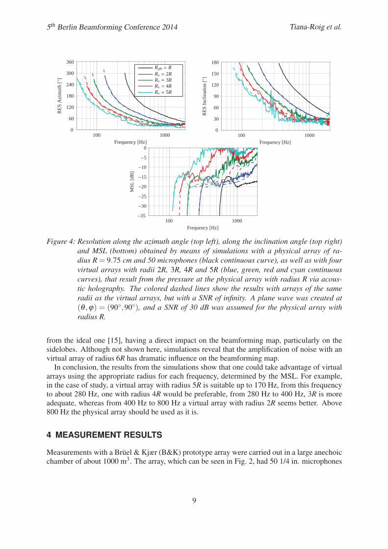
5th Berlin Beamforming Conference 2014 Tiana-Roig et al.
Frequency [Hz]
RES
Azi
mut
h[◦
]Rph = RRv = 2RRv = 3RRv = 4RRv = 5R
100 10000
60
120
180
240
300
360
Frequency [Hz]
RES
Incl
inat
ion
[◦]
100 10000
30
60
90
120
150
180
Frequency [Hz]
MSL
[dB
]
100 1000−35
−30
−25
−20
−15
−10
−5
0
Figure 4: Resolution along the azimuth angle (top left), along the inclination angle (top right)and MSL (bottom) obtained by means of simulations with a physical array of ra-dius R = 9.75 cm and 50 microphones (black continuous curve), as well as with fourvirtual arrays with radii 2R, 3R, 4R and 5R (blue, green, red and cyan continuouscurves), that result from the pressure at the physical array with radius R via acous-tic holography. The colored dashed lines show the results with arrays of the sameradii as the virtual arrays, but with a SNR of infinity. A plane wave was created at(θ ,ϕ) = (90◦,90◦), and a SNR of 30 dB was assumed for the physical array withradius R.
from the ideal one [15], having a direct impact on the beamforming map, particularly on thesidelobes. Although not shown here, simulations reveal that the amplification of noise with anvirtual array of radius 6R has dramatic influence on the beamforming map.
In conclusion, the results from the simulations show that one could take advantage of virtualarrays using the appropriate radius for each frequency, determined by the MSL. For example,in the case of study, a virtual array with radius 5R is suitable up to 170 Hz, from this frequencyto about 280 Hz, one with radius 4R would be preferable, from 280 Hz to 400 Hz, 3R is moreadequate, whereas from 400 Hz to 800 Hz a virtual array with radius 2R seems better. Above800 Hz the physical array should be used as it is.
4 MEASUREMENT RESULTS
Measurements with a Bruel & Kjær (B&K) prototype array were carried out in a large anechoicchamber of about 1000 m3. The array, which can be seen in Fig. 2, had 50 1/4 in. microphones
9

5th Berlin Beamforming Conference 2014 Tiana-Roig et al.
B&K Type 4935 flush-mounted on a rigid sphere and 11 video cameras. Its radius, R, was9.75 cm.
The set-up, shown in Fig. 5, consisted of a loudspeaker placed in the far field, at 5.8 m fromthe array. The loudspeaker height was 1 m and the array height 1.30 m. The array was placedsuch as the loudspeaker was detected at about (θ ,ϕ) = (90◦,90◦).
Figure 5: Measurement set-up.
The loudspeaker was fed with white noise. The signal level was adjusted so that the SNR atthe array microphones was about 30 dB for most of the frequency range, although the SNR atthe low frequencies was lower. The signal at each microphone was recorded with a B&K Pulseanalyzer for 10 s. The data was segmented in blocks of 1 s using a Hanning window and a 50%overlapping. For each block, the crosspectra between each microphone and a reference, whichwas chosen to be microphone number one, was computed. The averaged crosspectra were usedas input to conventional delay-and-sum beamforming. Besides, the data were used to predictthe pressure at several virtual radii Rv, at 2R, 3R, 4R and 5R, before applying beamforming,following the procedure indicated in Sec. 2.3. The resulting resolution for the azimuth andinclination angles, and the MSL with the physical and virtual arrays are shown in Fig. 6.
Both performance indicators follow the same trend observed in the simulations shown inFig. 4: the resolution improves towards the low frequencies with increasing virtual radius, andthe MSL is shifted towards the low frequencies, although its level increases with increasingvirtual radius. The reader should keep in mind that the simulations were carried out assum-ing a SNR of 30 dB, which was not exactly the case for the measurements, especially afterpostprocessing the data, and therefore, some deviations between simulations and results are ex-pected. In this regard, the MSL curves obtained with the virtual arrays are slightly better thanthe simulated ones.
These results confirm that the concept of virtual array can be used to enhance the performanceof the beamforming system at low frequencies, with an appropriate virtual radius depending onthe frequency. In this study, this makes it possible to extend the lower frequency of the physical
10

5th Berlin Beamforming Conference 2014 Tiana-Roig et al.
Frequency [Hz]
RES
Azi
mut
h[◦
]Rph = RRv = 2RRv = 3RRv = 4RRv = 5R
100 10000
60
120
180
240
300
360
Frequency [Hz]
RES
Incl
inat
ion
[◦]
100 10000
30
60
90
120
150
180
Frequency [Hz]
MSL
[dB
]
100 1000−35
−30
−25
−20
−15
−10
−5
0
Figure 6: Resolution along the azimuth angle (top left), resolution along the inclination angle(top right) and MSL (bottom) obtained by means of measurements with a rigid spher-ical array of radius R = 9.75 cm and 50 microphones (black continuous curve), aswell as the resulting resolution and MSL when considering four virtual spherical ar-rays with radii 2R, 3R, 4R and 5R (blue, green, red and cyan continuous curves), thatresult from the pressure at the physical array with radius R via acoustic holography.A plane wave was created at about (θ ,ϕ) = (90◦,90◦).
array down to about 55 Hz and 75 Hz in terms of resolution for the azimuth and the inclinationangles, respectively, and 110 Hz in terms of MSL, in comparison with the original 250 Hz,350 Hz and 550 Hz.
The advantage of combining acoustic holography and beamforming is further illustrated inFig. 7, where the beamforming map obtained with the physical array at 210 Hz is shown, to-gether with the maps obtained with virtual arrays with radii 2R, 3R and 4R. The larger the virtualradius, the clearer the map becomes, making it possible to localize better the sound source at itsactual position, (90◦,90◦).
11

5th Berlin Beamforming Conference 2014 Tiana-Roig et al.
Figure 7: Normalized beamforming outputs at 210 Hz measured with a rigid spherical arraywith 50 microphones and radius R = 9.75 cm (top left), and three virtual rigid spheri-cal arrays of radii 2R (top right), 3R (bottom left), and 4R (bottom middle), that resultfrom the pressure at the physical array with radius R via acoustic holography.
12

5th Berlin Beamforming Conference 2014 Tiana-Roig et al.
5 CONCLUSIONS
Beamforming with spherical arrays is a powerful tool to localize and identify sound sources ina three-dimensional sound field. However, the resulting maps are difficult to interpret at lowfrequencies because such frequencies imply poor directivity, in particular with delay-and-sumbeamforming. Inspired by the fact that the performance of the array would improve at lowfrequencies if a larger array was used, the present paper has presented a simple method thatconsists of predicting the pressure at a larger and virtual array by means of acoustic holography,and using it as input to the delay-and-sum beamforming procedure.
The performance of this combined approach has been assessed with two performance indica-tors, namely the resolution and the MSL. Both simulations and experimental results show thatthe resolution improves with increasing virtual radius, at the cost of the MSL, which is moresensitive to noise. This implies that the maximum virtual radius appropriate for each frequencyis mainly determined by the MSL.
The use of holography prior to delay-and-sum beamforming offers new possibilities withoutany additional cost. At low frequencies the concept of virtual array can be used to improvethe maps at such frequencies, while conventional beamforming can be applied directly at highfrequencies.
ACKNOWLEDGMENTS
The authors would like to thank Karim Haddad, Bruel & Kjær, for lending us the spherical arrayused in the measurements.
REFERENCES
[1] T. Abhayapala and Darren B. Ward. “Theory and design of high order sound field micro-phones using spherical microphone arrays.” IEEE ICASSP, II, 1949–1952, 2002.
[2] J. Meyer and G. Elko. “A highly scalable spherical microphone array based on an or-thonormal decomposition of the soundfield.” IEEE ICASSP, II, 1781–1784, 2002.
[3] M. Park and B. Rafaely. “Sound-field analysis by plane-wave decomposition using spher-ical microphone array.” J. Acoust. Soc. Am., 118(5), 3094–3103, 2005.
[4] B. Rafaely. “Plane-wave decomposition of the sound field on a sphere by spherical con-volution.” J. Acoust. Soc. Am., 116 (4), 2149–2157, 2004.
[5] B. Rafaely. “Phase-mode versus delay-and-sum spherical microphone array processing.”IEEE Signal Processing Letters, 12(10), 2005.
[6] B. Rafaely. “Spatial sampling and beamforming for spherical mircrophone arrays.” IEEEHSCMA, 2008.
[7] S. Favrot and M. Marschall. “Metrics for performance assessment of mixed-order am-bisonics spherical microphone arrays.” Proceedings of the AES 25th UK Conference,2012.
13

5th Berlin Beamforming Conference 2014 Tiana-Roig et al.
[8] M. Marschall, S. Favrot, and J. Buchholz. “Robustness of a mixed-order Ambisonics mi-crophone array for sound field reproduction.” Proceedings of the AES 132nd Convention,Budapest, Hungary, 2012.
[9] S. Moreau, J. Daniel, and S. Bertet. “3D sound field recording with higher order Am-bisonics - objective measurements and validation of a 4th order spherical microphone.”Proceedings of the AES 120th Convention, Paris, France, 2006.
[10] B. Rafaely. “Analysis and design of spherical microphone arrays.” IEEE Transactions onSpeech and Audio Processing, 13(1), 2005.
[11] B. Rafaely and B. Weiss. “Spatial aliasing in spherical microphone arrays.” IEEE Trans-actions on Signal Processing, 55(3), 2007.
[12] E. Tiana-Roig, A. Torras-Rosell, E. Fernandez-Grande, C.-H. Jeong, and F. Agerkvist.“Towards an enhanced performance of uniform circular arrays at low frequencies.” Inter-noise 2013, Innsbruck, Austria, 2013.
[13] E.G. Williams, N. Valdivia, P.C. Herdic and J. Klos. “Volumetric acoustic vector intensityimager.” J. Acoust. Soc. Am., 120(4), 1887–1897, 2006.
[14] E.G. Williams and K. Takashima. “Vector intensity reconstructions in a volume surround-ing a rigid spherical microphone array.” J. Acoust. Soc. Am., 127(2), 773–783, 2010.
[15] F. Jacobsen, G. Moreno-Pescador, E. Fernandez-Grande, and J. Hald. “Near field acousticholography with microphones on a rigid sphere (L).” J. Acoust. Soc. Am., 126(6), 3461–3464, 2011.
[16] F. Jacobsen and P. Juhl. Fundamentals of general linear acoustics. Wiley, 2013.
[17] F. Jacobsen, J. Hald, E. Fernandez-Grande, and G. Moreno. “Spherical near field acousticholography with microphones on a rigid sphere.” Acoustics’08, Paris, 2008.
[18] D. Johnson and D. Dudgeon. Array Signal Processing Concepts and Techniques. PrenticeHall, 1993.
[19] G. Arfken and H. Weber. Mathematical methods for physicists. Elsevier Academic Press,Burlington, MA, 2005.
[20] I. Sloan and R. Womersley. “External systems of points and numerical integration on thesphere.” Advances in Computational Mathematics, 21, 107–125, 2004.
14


www.elektro.dtu.dkDepartment of Electrical EngineeringAcoustic TechnologyTechnical University of DenmarkØrsteds PladsBuilding 348DK-2800 Kgs. LyngbyDenmarkTel: (+45) 45 25 38 00Fax: (+45) 45 93 16 34Email: [email protected]


