

Electric properties of halo nuclei using EFT
Daniel PhillipsOhio University
Work done in collaboration with H.-W. Hammer
Research supported by the US Department of Energy and the Deutsche Forschungsgemeinschaft
see also Rupak & Higa arXiv:1101.0207
arXiv:1001.1511 and “in preparation”

Outline

Outline
• Generalities: halo nuclei, experimental techniques
• Example 1: Halo EFT for Carbon-19
• Dissociation

Outline
• Generalities: halo nuclei, experimental techniques
• Example 1: Halo EFT for Carbon-19
• Dissociation
Shallow S-wave state
Outline
• Generalities: halo nuclei, experimental techniques
• Example 1: Halo EFT for Carbon-19
• Dissociation
• Example 2: Halo EFT for Beryllium-11
• Form factors
• E1 transition from s-state to p-state
• Dissociation
• Conclusion
Shallow S-wave state

Outline
• Generalities: halo nuclei, experimental techniques
• Example 1: Halo EFT for Carbon-19
• Dissociation
• Example 2: Halo EFT for Beryllium-11
• Form factors
• E1 transition from s-state to p-state
• Dissociation
• Conclusion
Shallow S-wave state
Shallow S-wave state Shallow P-wave state

Halo nuclei
Halo nuclei
• Here I define a halo nucleus as one in which the last nucleon (or nucleons) have a <r2>1/2 that is markedly larger than the range, R, of the interaction it has with the rest of the nucleus–the core.

Halo nuclei
• Here I define a halo nucleus as one in which the last nucleon (or nucleons) have a <r2>1/2 that is markedly larger than the range, R, of the interaction it has with the rest of the nucleus–the core.
• Typically R≡Rcore∼2-3 fm.

Halo nuclei
• Here I define a halo nucleus as one in which the last nucleon (or nucleons) have a <r2>1/2 that is markedly larger than the range, R, of the interaction it has with the rest of the nucleus–the core.
• Typically R≡Rcore∼2-3 fm.
• And since <r2> is related to the neutron separation energy we are looking for systems with neutron separation energies appreciably less than 1 MeV.
• Define Rhalo=<r2>1/2. Seek EFT expansion in Rcore/Rhalo.
• By this definition the deuteron is the lightest halo nucleus, and the pionless EFT for few-nucleon systems is a specific case of halo EFT.

Probing halo nuclei
• Typically produced in unstable beams.
• Neutron pickup reactions, e.g. (p,d), in inverse kinematics are one way to investigate
• Here my concern will be with electromagnetic probes.

Probing halo nuclei
• Typically produced in unstable beams.
• Neutron pickup reactions, e.g. (p,d), in inverse kinematics are one way to investigate
• Here my concern will be with electromagnetic probes.
• Coulomb dissociation: collide halo nucleus (we hope peripherally) with a high-Z nucleus
Bertulani, arXiv:0908.4307

Probing halo nuclei
• Typically produced in unstable beams.
• Neutron pickup reactions, e.g. (p,d), in inverse kinematics are one way to investigate
• Here my concern will be with electromagnetic probes.
• Coulomb dissociation: collide halo nucleus (we hope peripherally) with a high-Z nucleus
• Do with different Z, different nuclear sizes, different energies to test systematics
Bertulani, arXiv:0908.4307

From disintegration to E1 strength
dσC
2πbdb=
�
πL
�dEγ
EγnπL(Eγ , b)σπL
γ (Eγ)
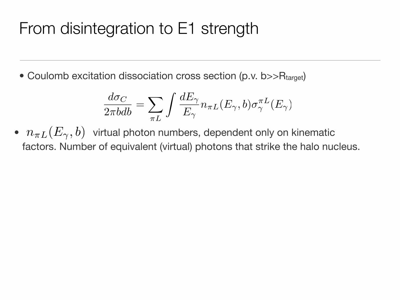
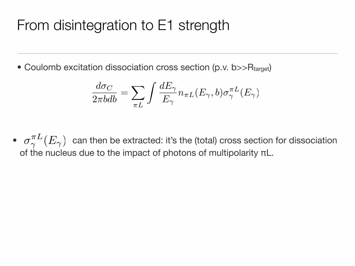
• Coulomb excitation dissociation cross section (p.v. b>>Rtarget)
From disintegration to E1 strength
• virtual photon numbers, dependent only on kinematic factors. Number of equivalent (virtual) photons that strike the halo nucleus.
dσC
2πbdb=
�
πL
�dEγ
EγnπL(Eγ , b)σπL
γ (Eγ)
nπL(Eγ , b)
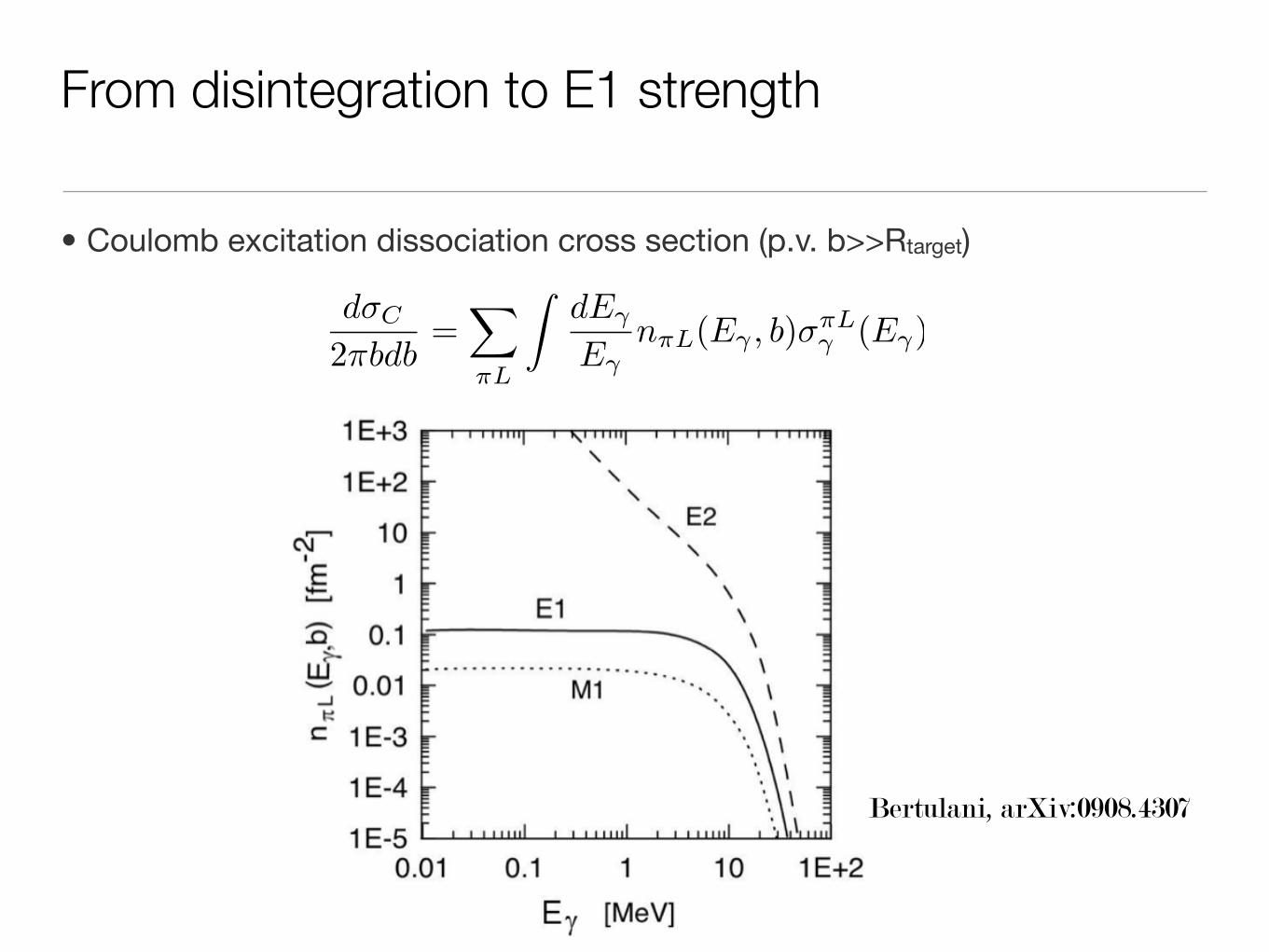
• Coulomb excitation dissociation cross section (p.v. b>>Rtarget)

From disintegration to E1 strength
• virtual photon numbers, dependent only on kinematic factors. Number of equivalent (virtual) photons that strike the halo nucleus.
• Virtual photon numbers computable in terms of relative velocity, equivalent photon frequency, impact parameter
dσC
2πbdb=
�
πL
�dEγ
EγnπL(Eγ , b)σπL
γ (Eγ)
nπL(Eγ , b)
• Coulomb excitation dissociation cross section (p.v. b>>Rtarget)
From disintegration to E1 strength
dσC
2πbdb=
�
πL
�dEγ
EγnπL(Eγ , b)σπL
γ (Eγ)
Bertulani, arXiv:0908.4307
• Coulomb excitation dissociation cross section (p.v. b>>Rtarget)
From disintegration to E1 strength
dσC
2πbdb=
�
πL
�dEγ
EγnπL(Eγ , b)σπL
γ (Eγ)
σπLγ (Eγ)
• Coulomb excitation dissociation cross section (p.v. b>>Rtarget)
• can then be extracted: it’s the (total) cross section for dissociation of the nucleus due to the impact of photons of multipolarity πL.

Our first halo nucleus: Carbon-19

Our first halo nucleus: Carbon-19
• 19C neutron separation energy=576 keV. Ground state=1/2+
• First excitation in 18C is 1.62 MeV above ground state
• Treat 1/2+ as s-wave halo state: 18C + n

Our first halo nucleus: Carbon-19
• 19C neutron separation energy=576 keV. Ground state=1/2+
• First excitation in 18C is 1.62 MeV above ground state
• Treat 1/2+ as s-wave halo state: 18C + n
• Blo/Bhi≈1/3⇒Rcore/Rhalo≈0.5

Our first halo nucleus: Carbon-19
• 19C neutron separation energy=576 keV. Ground state=1/2+
• First excitation in 18C is 1.62 MeV above ground state
• Treat 1/2+ as s-wave halo state: 18C + n
• Blo/Bhi≈1/3⇒Rcore/Rhalo≈0.5
• Data, including cut on impact parameter
Nakamura et al. (2003)

Our approach
Our approach
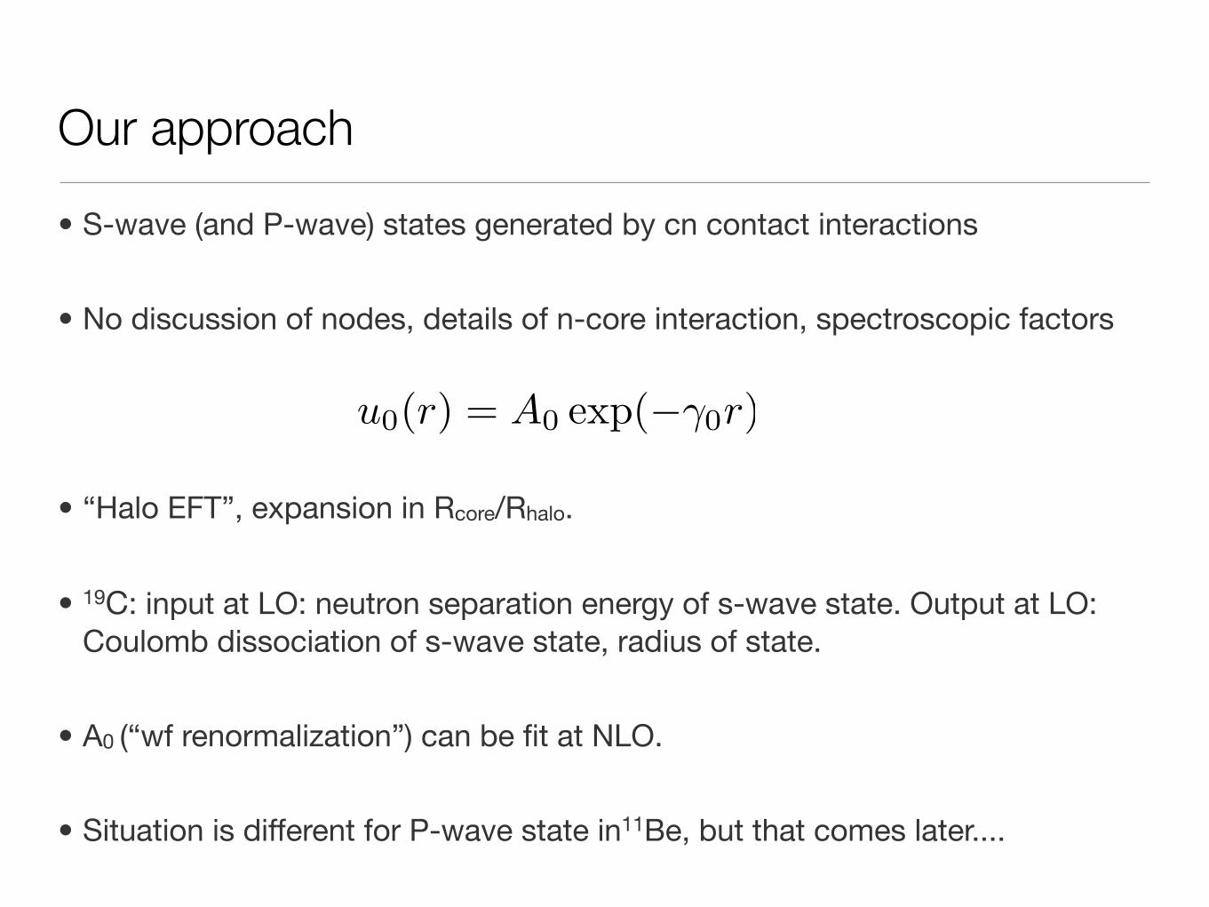
• S-wave (and P-wave) states generated by cn contact interactions

Our approach
• S-wave (and P-wave) states generated by cn contact interactions
• No discussion of nodes, details of n-core interaction, spectroscopic factors
u0(r) = A0 exp(−γ0r)

Our approach
• S-wave (and P-wave) states generated by cn contact interactions
• No discussion of nodes, details of n-core interaction, spectroscopic factors
• “Halo EFT”, expansion in Rcore/Rhalo.
u0(r) = A0 exp(−γ0r)

Our approach
• S-wave (and P-wave) states generated by cn contact interactions
• No discussion of nodes, details of n-core interaction, spectroscopic factors
• “Halo EFT”, expansion in Rcore/Rhalo.
• 19C: input at LO: neutron separation energy of s-wave state. Output at LO: Coulomb dissociation of s-wave state, radius of state.
• A0 (“wf renormalization”) can be fit at NLO.
u0(r) = A0 exp(−γ0r)
Our approach
• S-wave (and P-wave) states generated by cn contact interactions
• No discussion of nodes, details of n-core interaction, spectroscopic factors
• “Halo EFT”, expansion in Rcore/Rhalo.
• 19C: input at LO: neutron separation energy of s-wave state. Output at LO: Coulomb dissociation of s-wave state, radius of state.
• A0 (“wf renormalization”) can be fit at NLO.
• Situation is different for P-wave state in11Be, but that comes later....
u0(r) = A0 exp(−γ0r)

Lagrangian I: shallow s-wave state
L = c†�
i∂t +∇2
2M
�c + n†
�i∂t +
∇2
2m
�n
+σ†�η0
�i∂t +
∇2
2Mnc
�+ ∆0
�σ − g0[σn†c† + σ†nc]

Lagrangian I: shallow s-wave state
• c, n: “core”, “neutron” fields. c: boson, n: fermion.
• σ: s-wave field
L = c†�
i∂t +∇2
2M
�c + n†
�i∂t +
∇2
2m
�n
+σ†�η0
�i∂t +
∇2
2Mnc
�+ ∆0
�σ − g0[σn†c† + σ†nc]

Lagrangian I: shallow s-wave state
• c, n: “core”, “neutron” fields. c: boson, n: fermion.
• σ: s-wave field
• Minimal substitution→dominant EM interactions; other terms suppressed by additional powers of Rcore/Rhalo
• ...if coefficients natural. But that’s a testable assumption.
L = c†�
i∂t +∇2
2M
�c + n†
�i∂t +
∇2
2m
�n
+σ†�η0
�i∂t +
∇2
2Mnc
�+ ∆0
�σ − g0[σn†c† + σ†nc]

Dressing the s-wave state
= +
Kaplan, Savage, Wise; van Kolck; Gegelia; Birse, Richardson, McGovern

• σnc coupling g0 of order Rhalo, nc loop of order 1/Rhalo. Therefore need to sum all bubbles:
Dressing the s-wave state
= +
Kaplan, Savage, Wise; van Kolck; Gegelia; Birse, Richardson, McGovern

• σnc coupling g0 of order Rhalo, nc loop of order 1/Rhalo. Therefore need to sum all bubbles:
Dσ(p) =1
∆0 + η0[p0 − p2/(2Mnc)]− Σσ(p)
Dressing the s-wave state
= +
Kaplan, Savage, Wise; van Kolck; Gegelia; Birse, Richardson, McGovern

• σnc coupling g0 of order Rhalo, nc loop of order 1/Rhalo. Therefore need to sum all bubbles:
Dσ(p) =1
∆0 + η0[p0 − p2/(2Mnc)]− Σσ(p)
Dressing the s-wave state
= +
Kaplan, Savage, Wise; van Kolck; Gegelia; Birse, Richardson, McGovern
Σσ(p) = −g20mR
2π
�µ + i
�
2mR
�p0 −
p2
2Mnc+ iη
��(PDS)

• σnc coupling g0 of order Rhalo, nc loop of order 1/Rhalo. Therefore need to sum all bubbles:
Dσ(p) =1
∆0 + η0[p0 − p2/(2Mnc)]− Σσ(p)
Dressing the s-wave state
= +
t =2π
mR
11a0− 1
2r0k2 + ik
Kaplan, Savage, Wise; van Kolck; Gegelia; Birse, Richardson, McGovern
Σσ(p) = −g20mR
2π
�µ + i
�
2mR
�p0 −
p2
2Mnc+ iη
��(PDS)
+ regularDσ(p) =2πγ0
m2Rg2
0
11− r0γ0
1p0 − p2
2Mnc+ B0

Predicting dissociationc.f. Chen, Savage (1999)

Predicting dissociation
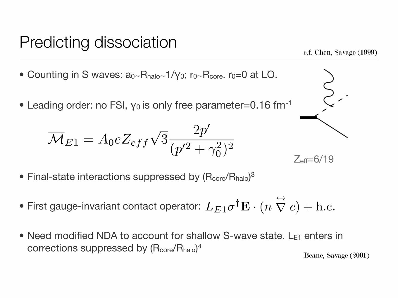
• Counting in S waves: a0∼Rhalo∼1/γ0; r0∼Rcore. r0=0 at LO.
c.f. Chen, Savage (1999)

Predicting dissociation
• Counting in S waves: a0∼Rhalo∼1/γ0; r0∼Rcore. r0=0 at LO.
• Leading order: no FSI, γ0 is only free parameter=0.16 fm-1
c.f. Chen, Savage (1999)

Predicting dissociation
• Counting in S waves: a0∼Rhalo∼1/γ0; r0∼Rcore. r0=0 at LO.
• Leading order: no FSI, γ0 is only free parameter=0.16 fm-1
M =eQcg02mR
γ20 +
�p� − m
Mnck�2
c.f. Chen, Savage (1999)

Predicting dissociation
• Counting in S waves: a0∼Rhalo∼1/γ0; r0∼Rcore. r0=0 at LO.
• Leading order: no FSI, γ0 is only free parameter=0.16 fm-1
ME1 = A0eZeff
√3
2p�
(p�2 + γ20)2
c.f. Chen, Savage (1999)
Zeff=6/19

Predicting dissociation
• Counting in S waves: a0∼Rhalo∼1/γ0; r0∼Rcore. r0=0 at LO.
• Leading order: no FSI, γ0 is only free parameter=0.16 fm-1
• Final-state interactions suppressed by (Rcore/Rhalo)3
ME1 = A0eZeff
√3
2p�
(p�2 + γ20)2
c.f. Chen, Savage (1999)
Zeff=6/19

Predicting dissociation
• Counting in S waves: a0∼Rhalo∼1/γ0; r0∼Rcore. r0=0 at LO.
• Leading order: no FSI, γ0 is only free parameter=0.16 fm-1
• Final-state interactions suppressed by (Rcore/Rhalo)3
• First gauge-invariant contact operator: LE1σ†E · (n
↔∇ c) + h.c.
ME1 = A0eZeff
√3
2p�
(p�2 + γ20)2
c.f. Chen, Savage (1999)
Zeff=6/19
Predicting dissociation
• Counting in S waves: a0∼Rhalo∼1/γ0; r0∼Rcore. r0=0 at LO.
• Leading order: no FSI, γ0 is only free parameter=0.16 fm-1
• Final-state interactions suppressed by (Rcore/Rhalo)3
• First gauge-invariant contact operator:
• Need modified NDA to account for shallow S-wave state. LE1 enters in corrections suppressed by (Rcore/Rhalo)4
LE1σ†E · (n
↔∇ c) + h.c.
ME1 = A0eZeff
√3
2p�
(p�2 + γ20)2
c.f. Chen, Savage (1999)
Beane, Savage (2001)
Zeff=6/19

Predicting dissociation
• Counting in S waves: a0∼Rhalo∼1/γ0; r0∼Rcore. r0=0 at LO.
• Leading order: no FSI, γ0 is only free parameter=0.16 fm-1
• Final-state interactions suppressed by (Rcore/Rhalo)3
• First gauge-invariant contact operator:
• Need modified NDA to account for shallow S-wave state. LE1 enters in corrections suppressed by (Rcore/Rhalo)4
• Consistent with short-distance piece of FSI loop due to P-wave interactions
LE1σ†E · (n
↔∇ c) + h.c.
ME1 = A0eZeff
√3
2p�
(p�2 + γ20)2
c.f. Chen, Savage (1999)
Beane, Savage (2001)
Zeff=6/19

ResultsData: Nakamura et al., PRL, 1999
ResultsData: Nakamura et al., PRL, 1999
• Observable is dB(E1)/dE: E1 strength for transition to a core + neutron state, per unit energy, as function of energy (momentum) of the outgoing nc pair
• Multiply by NE1(Eγ):
ResultsData: Nakamura et al., PRL, 1999
• Observable is dB(E1)/dE: E1 strength for transition to a core + neutron state, per unit energy, as function of energy (momentum) of the outgoing nc pair

∼ A20 =
2γ0
1− r0γ0
• Multiply by NE1(Eγ):
• r0 fixed from fitting height of peak at NLO
• γ0 determines peak position
ResultsData: Nakamura et al., PRL, 1999
• Observable is dB(E1)/dE: E1 strength for transition to a core + neutron state, per unit energy, as function of energy (momentum) of the outgoing nc pair
• Determine S-wave 18C-n scattering parameters from dissociation data.

S-wave form factor
-iΓc(q)
q

S-wave form factor
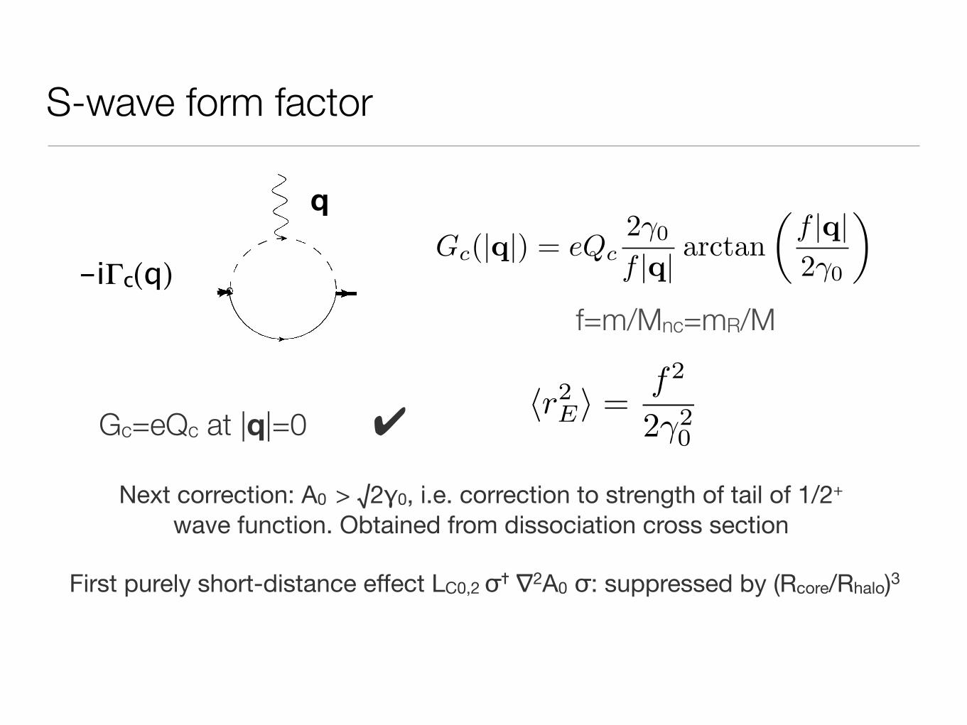
Gc(|q|) = eQc2γ0
f |q| arctan�
f |q|2γ0
�
f=m/Mnc=mR/M
-iΓc(q)
q

S-wave form factor
Gc=eQc at |q|=0 ✔
Gc(|q|) = eQc2γ0
f |q| arctan�
f |q|2γ0
�
f=m/Mnc=mR/M
-iΓc(q)
q

�r2E� =
f2
2γ20
S-wave form factor
Gc=eQc at |q|=0 ✔
Gc(|q|) = eQc2γ0
f |q| arctan�
f |q|2γ0
�
f=m/Mnc=mR/M
-iΓc(q)
q

�r2E� =
f2
2γ20
S-wave form factor
Gc=eQc at |q|=0 ✔
Gc(|q|) = eQc2γ0
f |q| arctan�
f |q|2γ0
�
f=m/Mnc=mR/M
-iΓc(q)
q
Next correction: A0 > √2γ0, i.e. correction to strength of tail of 1/2+ wave function. Obtained from dissociation cross section
�r2E� =
f2
2γ20
S-wave form factor
Gc=eQc at |q|=0 ✔
Gc(|q|) = eQc2γ0
f |q| arctan�
f |q|2γ0
�
f=m/Mnc=mR/M
-iΓc(q)
q
Next correction: A0 > √2γ0, i.e. correction to strength of tail of 1/2+ wave function. Obtained from dissociation cross section
First purely short-distance effect LC0,2 σ✝ ∇2A0 σ: suppressed by (Rcore/Rhalo)3
(<rE2>C19-<rE2>C18)1/2=0.23 + 0.08 fm
LO NLO

Beryllium-11 as a (one-neutron)* halo nucleus
*could also be thought of as a 3n halo

Beryllium-11 as a (one-neutron)* halo nucleus
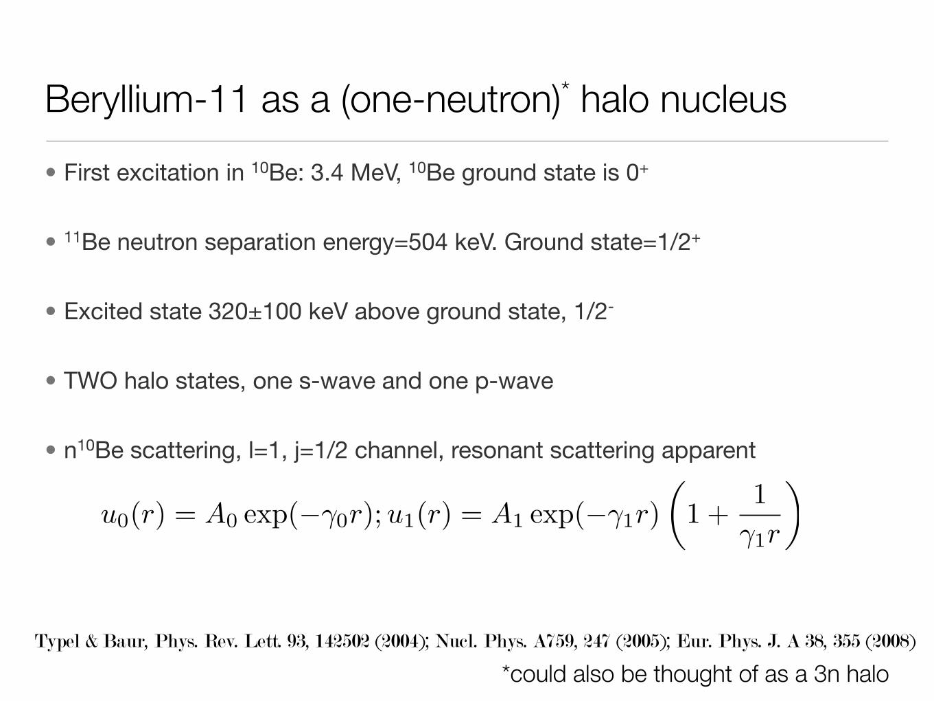
• First excitation in 10Be: 3.4 MeV, 10Be ground state is 0+
• 11Be neutron separation energy=504 keV. Ground state=1/2+
• Excited state 320±100 keV above ground state, 1/2-
*could also be thought of as a 3n halo

Beryllium-11 as a (one-neutron)* halo nucleus
• First excitation in 10Be: 3.4 MeV, 10Be ground state is 0+
• 11Be neutron separation energy=504 keV. Ground state=1/2+
• Excited state 320±100 keV above ground state, 1/2-
• TWO halo states, one s-wave and one p-wave
*could also be thought of as a 3n halo
Beryllium-11 as a (one-neutron)* halo nucleus
• First excitation in 10Be: 3.4 MeV, 10Be ground state is 0+
• 11Be neutron separation energy=504 keV. Ground state=1/2+
• Excited state 320±100 keV above ground state, 1/2-
• TWO halo states, one s-wave and one p-wave
• n10Be scattering, l=1, j=1/2 channel, resonant scattering apparent
*could also be thought of as a 3n haloTypel & Baur, Phys. Rev. Lett. 93, 142502 (2004); Nucl. Phys. A759, 247 (2005); Eur. Phys. J. A 38, 355 (2008)
u0(r) = A0 exp(−γ0r);u1(r) = A1 exp(−γ1r)�
1 +1
γ1r
�

Beryllium-11 as a (one-neutron)* halo nucleus
• First excitation in 10Be: 3.4 MeV, 10Be ground state is 0+
• 11Be neutron separation energy=504 keV. Ground state=1/2+
• Excited state 320±100 keV above ground state, 1/2-
• TWO halo states, one s-wave and one p-wave
• n10Be scattering, l=1, j=1/2 channel, resonant scattering apparent
• Blo/Bhi≈1/6⇒Rcore/Rhalo≈0.4
*could also be thought of as a 3n haloTypel & Baur, Phys. Rev. Lett. 93, 142502 (2004); Nucl. Phys. A759, 247 (2005); Eur. Phys. J. A 38, 355 (2008)
u0(r) = A0 exp(−γ0r);u1(r) = A1 exp(−γ1r)�
1 +1
γ1r
�

Electromagnetic properties

Electromagnetic properties
• B(E1)(1/2+→1/2-)=0.105(12) e2fm2 from intermediate-energy Coulomb excitation
(Summers et al., 2007)
• B(E1)(1/2+→1/2-)=0.116(12) e2fm2 from lifetime measurements (Millener et al., 1983)

Electromagnetic properties
• B(E1)(1/2+→1/2-)=0.105(12) e2fm2 from intermediate-energy Coulomb excitation
(Summers et al., 2007)
• B(E1)(1/2+→1/2-)=0.116(12) e2fm2 from lifetime measurements (Millener et al., 1983)
Coulomb-induced breakup of 11Be, Palit et al. (2003), c.f. Fukuda et al. (2004)

Electromagnetic properties
• B(E1)(1/2+→1/2-)=0.105(12) e2fm2 from intermediate-energy Coulomb excitation
(Summers et al., 2007)
• B(E1)(1/2+→1/2-)=0.116(12) e2fm2 from lifetime measurements (Millener et al., 1983)
B(E1, li) = [Z(1)effe]2
34π
�r2�li
Non-energy-weighted sum rule:
<r2>1/2=5.7(4) fm
Zeff=4/11
c.f. atomic-physics measurement of radiiNoerterhaueser et al., PRL (2009)
Coulomb-induced breakup of 11Be, Palit et al. (2003), c.f. Fukuda et al. (2004)

Lagrangian II: shallow S- and P-states
• c, n: “core”, “neutron” fields. c: boson, n: fermion.
• σ, πj: S-wave and P-wave fields
• Compute power of non-minimal EM couplings by NDA with rescaled fields.
L = c†�
i∂t +∇2
2M
�c + n†
�i∂t +
∇2
2m
�n
+σ†�η0
�i∂t +
∇2
2Mnc
�+ ∆0
�σ + π†
j
�η1
�i∂t +
∇2
2Mnc
�+ ∆1
�πj
−g0
�σn†c† + σ†nc
�− g1
2
�π†
j (n↔
i∇j c) + (c†↔
i∇j n†)πj
�
−g1
2M −m
Mnc
�π†
j
→i∇j (nc)−
↔i∇j (n†c†)πj
�+ . . . ,

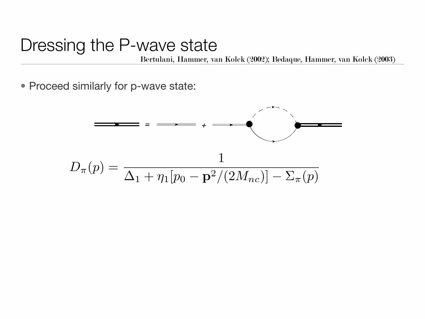
Dressing the P-wave state
= +
Bertulani, Hammer, van Kolck (2002); Bedaque, Hammer, van Kolck (2003)

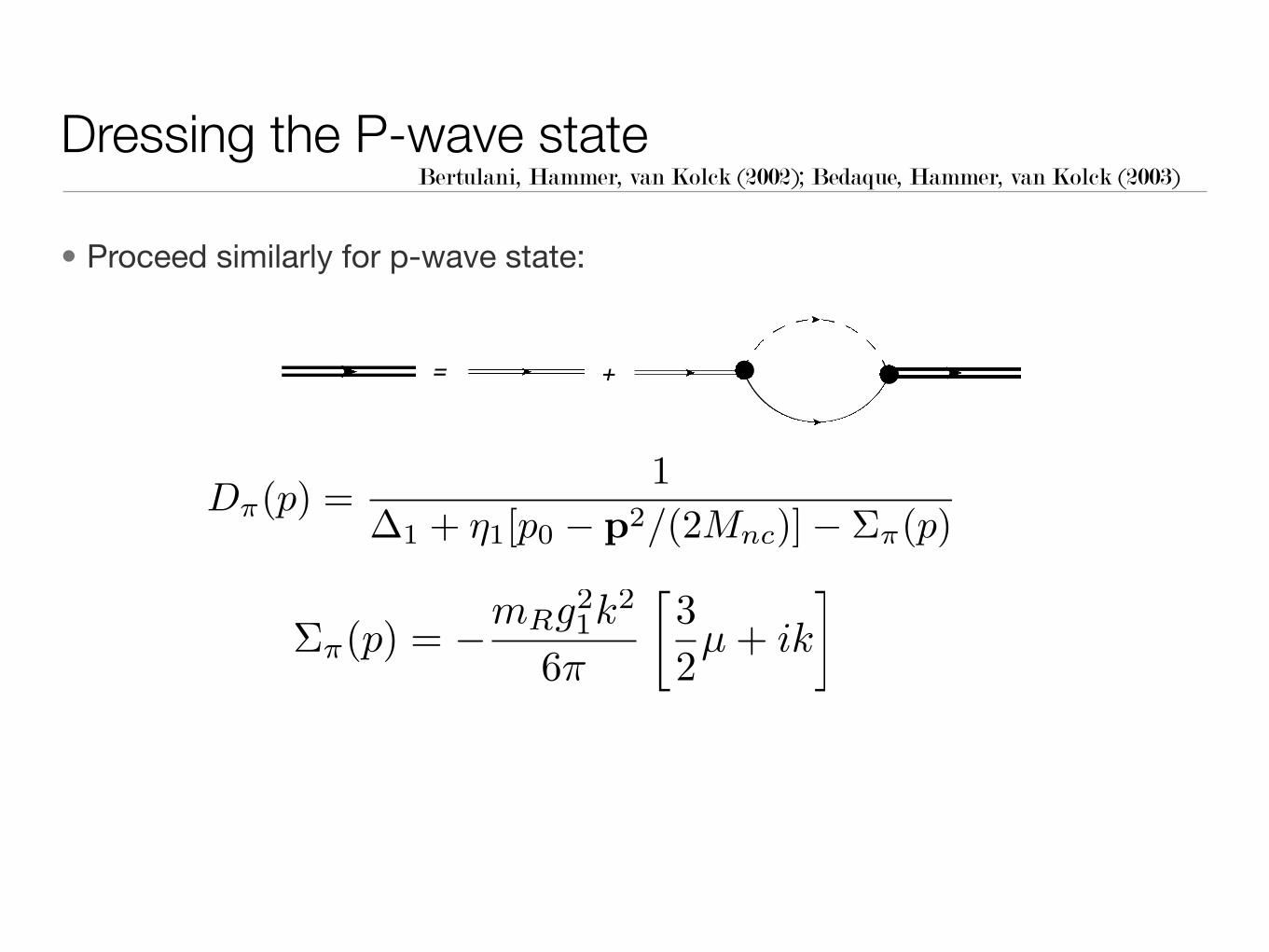
• Proceed similarly for p-wave state:
Dressing the P-wave state
= +
Bertulani, Hammer, van Kolck (2002); Bedaque, Hammer, van Kolck (2003)
• Proceed similarly for p-wave state:
Dressing the P-wave state
= +
Bertulani, Hammer, van Kolck (2002); Bedaque, Hammer, van Kolck (2003)
Dπ(p) =1
∆1 + η1[p0 − p2/(2Mnc)]− Σπ(p)
• Proceed similarly for p-wave state:
Dressing the P-wave state
= +
Bertulani, Hammer, van Kolck (2002); Bedaque, Hammer, van Kolck (2003)
Σπ(p) = −mRg21k2
6π
�32µ + ik
�
Dπ(p) =1
∆1 + η1[p0 − p2/(2Mnc)]− Σπ(p)
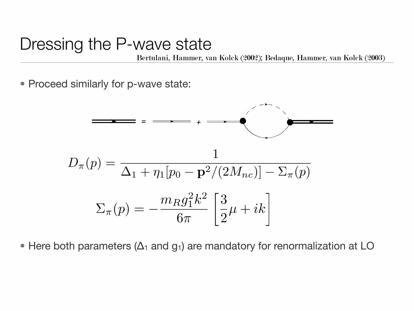
• Proceed similarly for p-wave state:
• Here both parameters (Δ1 and g1) are mandatory for renormalization at LO
Dressing the P-wave state
= +
Bertulani, Hammer, van Kolck (2002); Bedaque, Hammer, van Kolck (2003)
Σπ(p) = −mRg21k2
6π
�32µ + ik
�
Dπ(p) =1
∆1 + η1[p0 − p2/(2Mnc)]− Σπ(p)
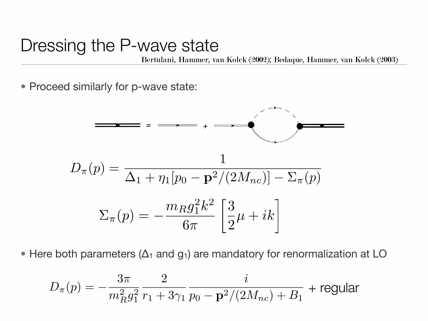
• Proceed similarly for p-wave state:
• Here both parameters (Δ1 and g1) are mandatory for renormalization at LO
Dressing the P-wave state
= +
Bertulani, Hammer, van Kolck (2002); Bedaque, Hammer, van Kolck (2003)
Σπ(p) = −mRg21k2
6π
�32µ + ik
�
+ regularDπ(p) = − 3π
m2Rg2
1
2r1 + 3γ1
i
p0 − p2/(2Mnc) + B1
Dπ(p) =1
∆1 + η1[p0 − p2/(2Mnc)]− Σπ(p)
Fixing P-wave parameters

Fixing P-wave parameters
• Input at LO: neutron separation energy of s-wave and p-wave state, B0=504 keV, B1=184 keV
• ⇒γ0=0.15 fm-1; γ1=0.09 fm-1 both ∼1/Rhalo

Fixing P-wave parameters
• Input at LO: neutron separation energy of s-wave and p-wave state, B0=504 keV, B1=184 keV
• ⇒γ0=0.15 fm-1; γ1=0.09 fm-1 both ∼1/Rhalo
• Also need to fix r1 at LO, we anticipate r1∼1/Rcore

Fixing P-wave parameters
• Input at LO: neutron separation energy of s-wave and p-wave state, B0=504 keV, B1=184 keV
• ⇒γ0=0.15 fm-1; γ1=0.09 fm-1 both ∼1/Rhalo
• Also need to fix r1 at LO, we anticipate r1∼1/Rcore
• k3 cot δ1=-1/2 r1 (k2 + γ12) at LO; (k∼γ1⇒r1k2 >> γ13)

Fixing P-wave parameters
• Input at LO: neutron separation energy of s-wave and p-wave state, B0=504 keV, B1=184 keV
• ⇒γ0=0.15 fm-1; γ1=0.09 fm-1 both ∼1/Rhalo
• Also need to fix r1 at LO, we anticipate r1∼1/Rcore
• k3 cot δ1=-1/2 r1 (k2 + γ12) at LO; (k∼γ1⇒r1k2 >> γ13)
• Note: a1∼Rhalo2 Rcore, c.f. original scenario of Bertulani et al. a1∼Rhalo3
• We are going to use the B(E1:1/2+→1/2-) strength to fix r1.
• No propagation of experimental errors here, but it’s easy to do

+
Irreducible S-to-P vertex: bound-to-bound transition
-iΓjµ(k) k0=ω
i
jq
k

+
Irreducible S-to-P vertex: bound-to-bound transition
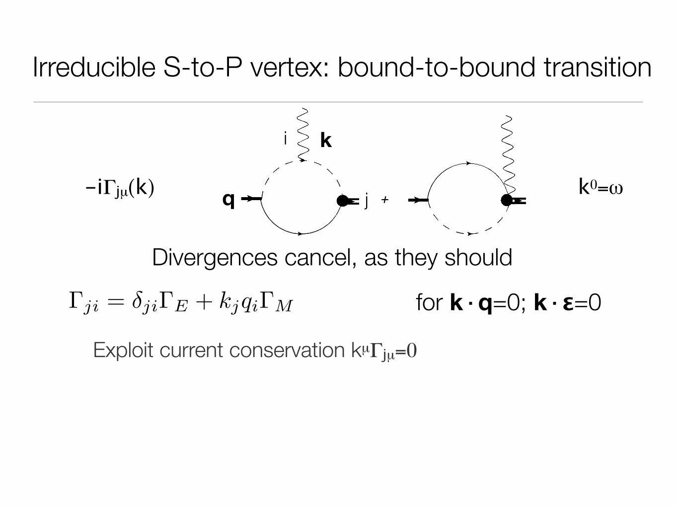
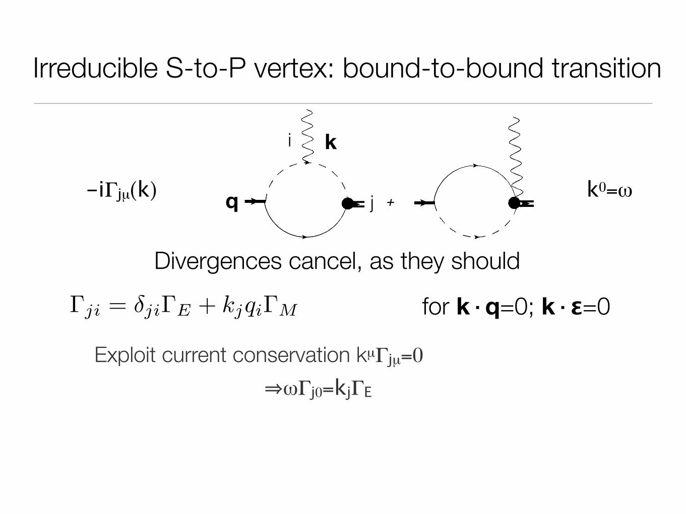
Divergences cancel, as they should
-iΓjµ(k) k0=ω
i
jq
k

+
Irreducible S-to-P vertex: bound-to-bound transition
Divergences cancel, as they should
Γji = δjiΓE + kjqiΓM for k·q=0; k·ε=0
-iΓjµ(k) k0=ω
i
jq
k
+
Irreducible S-to-P vertex: bound-to-bound transition
Divergences cancel, as they should
Γji = δjiΓE + kjqiΓM for k·q=0; k·ε=0
Exploit current conservation kµΓjµ=0
-iΓjµ(k) k0=ω
i
jq
k
+
Irreducible S-to-P vertex: bound-to-bound transition
Divergences cancel, as they should
Γji = δjiΓE + kjqiΓM for k·q=0; k·ε=0
Exploit current conservation kµΓjµ=0
⇒ωΓj0=kjΓE
-iΓjµ(k) k0=ω
i
jq
k

+
Γj0(k) ∼�
d3ru1(r)
rY1j(r̂)eik·r u0(r)
r
Irreducible S-to-P vertex: bound-to-bound transition
Divergences cancel, as they should
Γji = δjiΓE + kjqiΓM for k·q=0; k·ε=0
Exploit current conservation kµΓjµ=0
⇒ωΓj0=kjΓE
-iΓjµ(k) k0=ω
i
jq
k

→ kj
�dru1(r)ru0(r) as |k|→ 0
+
Γj0(k) ∼�
d3ru1(r)
rY1j(r̂)eik·r u0(r)
r
Irreducible S-to-P vertex: bound-to-bound transition
Divergences cancel, as they should
Γji = δjiΓE + kjqiΓM for k·q=0; k·ε=0
Exploit current conservation kµΓjµ=0
⇒ωΓj0=kjΓE
-iΓjµ(k) k0=ω
i
jq
k
E1 matrix element

Converting to result for S-to-P transition
B(E1) =14π
�Γ̄E
ω
�2
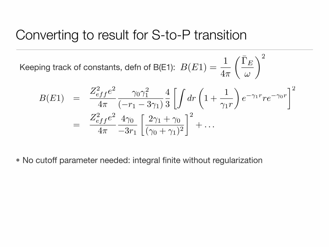
Keeping track of constants, defn of B(E1):

Converting to result for S-to-P transition
B(E1) =Z2
effe2
4π
γ0γ21
(−r1 − 3γ1)43
��dr
�1 +
1γ1r
�e−γ1rre−γ0r
�2
=Z2
effe2
4π
4γ0
−3r1
�2γ1 + γ0
(γ0 + γ1)2
�2
+ . . .
B(E1) =14π
�Γ̄E
ω
�2
Keeping track of constants, defn of B(E1):
Converting to result for S-to-P transition
• No cutoff parameter needed: integral finite without regularization
B(E1) =Z2
effe2
4π
γ0γ21
(−r1 − 3γ1)43
��dr
�1 +
1γ1r
�e−γ1rre−γ0r
�2
=Z2
effe2
4π
4γ0
−3r1
�2γ1 + γ0
(γ0 + γ1)2
�2
+ . . .
B(E1) =14π
�Γ̄E
ω
�2
Keeping track of constants, defn of B(E1):

Converting to result for S-to-P transition
• No cutoff parameter needed: integral finite without regularization
• Numbers: BLO(E1)=0.106 e2fm2 , yields r1=-0.66 fm-1
• NLO corrections from A0 and γ1/r1 corrections to A1
• Also first contribution of physics at scale Rcore occurs at NLO
B(E1) =Z2
effe2
4π
γ0γ21
(−r1 − 3γ1)43
��dr
�1 +
1γ1r
�e−γ1rre−γ0r
�2
=Z2
effe2
4π
4γ0
−3r1
�2γ1 + γ0
(γ0 + γ1)2
�2
+ . . .
B(E1) =14π
�Γ̄E
ω
�2
Keeping track of constants, defn of B(E1):

Computing dissociation: γE1 + 11Be→10Be + n
Computing dissociation: γE1 + 11Be→10Be + n
• Note that final state can be spin-1/2 or spin-3/2: final-state interactions are “nautral” in the spin-3/2 channel, i.e. suppressed by three orders.

Computing dissociation: γE1 + 11Be→10Be + n
• Note that final state can be spin-1/2 or spin-3/2: final-state interactions are “nautral” in the spin-3/2 channel, i.e. suppressed by three orders.
• FSI in spin-1/2 channel: stronger, but “kinematic” nature of p-wave state implies interaction still perturbative away from resonance:
k3 cot δ1=-1/2 r1 (k2 + γ12) ⇒ δ1 ∼ Rcore/Rhalo if k ∼ 1/Rhalo ∼ γ1.

Computing dissociation: γE1 + 11Be→10Be + n
• Note that final state can be spin-1/2 or spin-3/2: final-state interactions are “nautral” in the spin-3/2 channel, i.e. suppressed by three orders.
• FSI in spin-1/2 channel: stronger, but “kinematic” nature of p-wave state implies interaction still perturbative away from resonance:
!
LO NLO
k3 cot δ1=-1/2 r1 (k2 + γ12) ⇒ δ1 ∼ Rcore/Rhalo if k ∼ 1/Rhalo ∼ γ1.

Computing dissociation: γE1 + 11Be→10Be + n
• Note that final state can be spin-1/2 or spin-3/2: final-state interactions are “nautral” in the spin-3/2 channel, i.e. suppressed by three orders.
• FSI in spin-1/2 channel: stronger, but “kinematic” nature of p-wave state implies interaction still perturbative away from resonance:
• Also get corrections to A0 (a.k.a. wf renormalization) at NLO
!
LO NLO
k3 cot δ1=-1/2 r1 (k2 + γ12) ⇒ δ1 ∼ Rcore/Rhalo if k ∼ 1/Rhalo ∼ γ1.

Coulomb dissociation: formulae
dB(E1)dE
= e2Z2eff
mR
2π2A2
0
�p�3[2p�3 cot(δ(1/2)(p�)) + γ3
0 + 3γ0p�2]2
[p�6 + p�6 cot2(δ(1/2)(p�))](p�2 + γ20)4
+8p�3
(p�2 + γ20)4
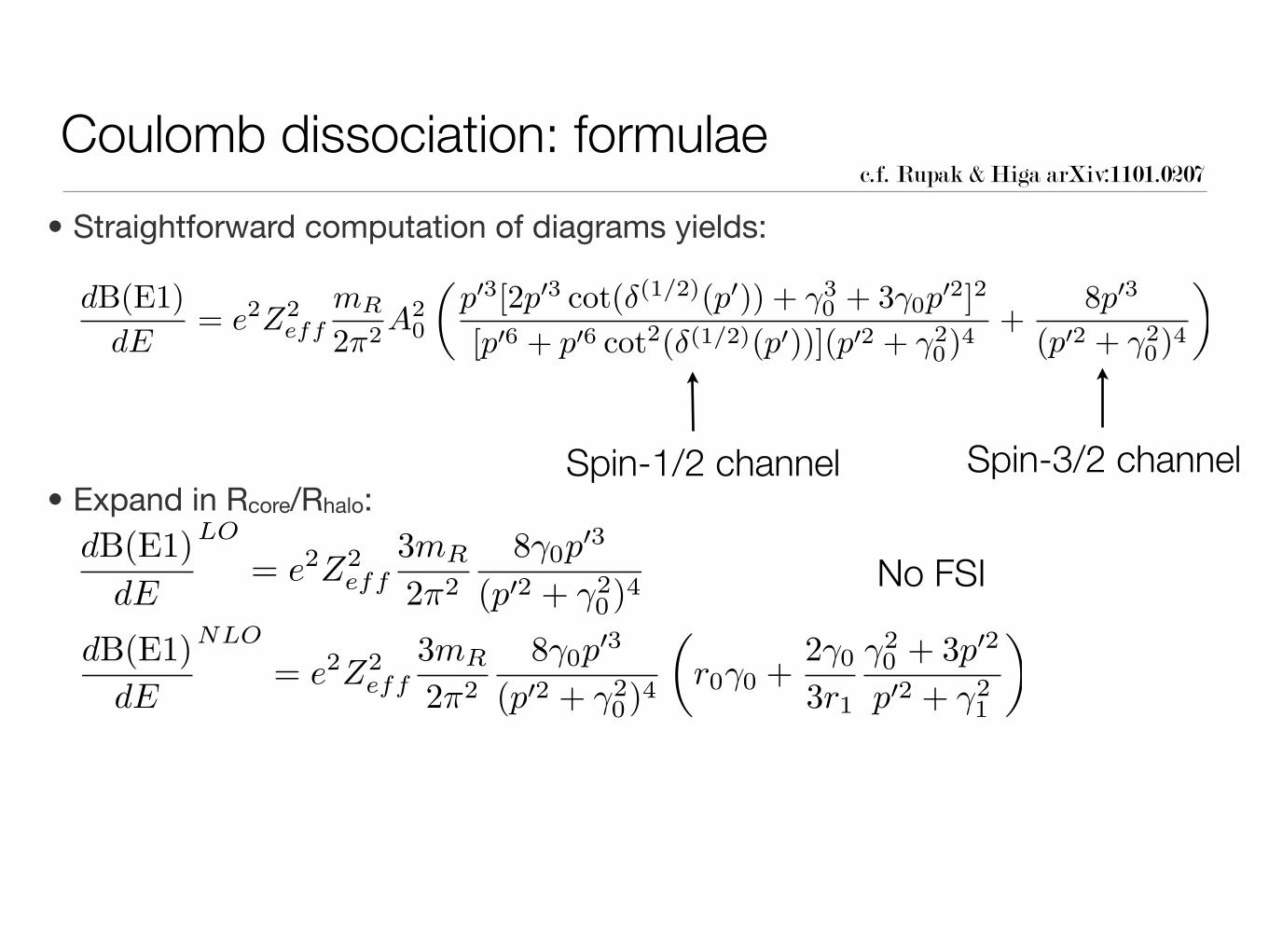
�• Straightforward computation of diagrams yields:
c.f. Rupak & Higa arXiv:1101.0207

Coulomb dissociation: formulae
dB(E1)dE
= e2Z2eff
mR
2π2A2
0
�p�3[2p�3 cot(δ(1/2)(p�)) + γ3
0 + 3γ0p�2]2
[p�6 + p�6 cot2(δ(1/2)(p�))](p�2 + γ20)4
+8p�3
(p�2 + γ20)4
�• Straightforward computation of diagrams yields:
Spin-1/2 channel Spin-3/2 channel
c.f. Rupak & Higa arXiv:1101.0207

Coulomb dissociation: formulae
dB(E1)dE
= e2Z2eff
mR
2π2A2
0
�p�3[2p�3 cot(δ(1/2)(p�)) + γ3
0 + 3γ0p�2]2
[p�6 + p�6 cot2(δ(1/2)(p�))](p�2 + γ20)4
+8p�3
(p�2 + γ20)4
�• Straightforward computation of diagrams yields:
• Expand in Rcore/Rhalo:Spin-1/2 channel Spin-3/2 channel
c.f. Rupak & Higa arXiv:1101.0207

Coulomb dissociation: formulae
dB(E1)dE
= e2Z2eff
mR
2π2A2
0
�p�3[2p�3 cot(δ(1/2)(p�)) + γ3
0 + 3γ0p�2]2
[p�6 + p�6 cot2(δ(1/2)(p�))](p�2 + γ20)4
+8p�3
(p�2 + γ20)4
�
dB(E1)dE
LO
= e2Z2eff
3mR
2π2
8γ0p�3
(p�2 + γ20)4 No FSI
• Straightforward computation of diagrams yields:
• Expand in Rcore/Rhalo:Spin-1/2 channel Spin-3/2 channel
c.f. Rupak & Higa arXiv:1101.0207
Coulomb dissociation: formulae
dB(E1)dE
= e2Z2eff
mR
2π2A2
0
�p�3[2p�3 cot(δ(1/2)(p�)) + γ3
0 + 3γ0p�2]2
[p�6 + p�6 cot2(δ(1/2)(p�))](p�2 + γ20)4
+8p�3
(p�2 + γ20)4
�
dB(E1)dE
LO
= e2Z2eff
3mR
2π2
8γ0p�3
(p�2 + γ20)4 No FSI
dB(E1)dE
NLO
= e2Z2eff
3mR
2π2
8γ0p�3
(p�2 + γ20)4
�r0γ0 +
2γ0
3r1
γ20 + 3p�2
p�2 + γ21
�
• Straightforward computation of diagrams yields:
• Expand in Rcore/Rhalo:Spin-1/2 channel Spin-3/2 channel
c.f. Rupak & Higa arXiv:1101.0207

Coulomb dissociation: formulae
dB(E1)dE
= e2Z2eff
mR
2π2A2
0
�p�3[2p�3 cot(δ(1/2)(p�)) + γ3
0 + 3γ0p�2]2
[p�6 + p�6 cot2(δ(1/2)(p�))](p�2 + γ20)4
+8p�3
(p�2 + γ20)4
�
dB(E1)dE
LO
= e2Z2eff
3mR
2π2
8γ0p�3
(p�2 + γ20)4 No FSI
dB(E1)dE
NLO
= e2Z2eff
3mR
2π2
8γ0p�3
(p�2 + γ20)4
�r0γ0 +
2γ0
3r1
γ20 + 3p�2
p�2 + γ21
�
Wf renormalization
• Straightforward computation of diagrams yields:
• Expand in Rcore/Rhalo:Spin-1/2 channel Spin-3/2 channel
c.f. Rupak & Higa arXiv:1101.0207

Coulomb dissociation: formulae
dB(E1)dE
= e2Z2eff
mR
2π2A2
0
�p�3[2p�3 cot(δ(1/2)(p�)) + γ3
0 + 3γ0p�2]2
[p�6 + p�6 cot2(δ(1/2)(p�))](p�2 + γ20)4
+8p�3
(p�2 + γ20)4
�
dB(E1)dE
LO
= e2Z2eff
3mR
2π2
8γ0p�3
(p�2 + γ20)4 No FSI
dB(E1)dE
NLO
= e2Z2eff
3mR
2π2
8γ0p�3
(p�2 + γ20)4
�r0γ0 +
2γ0
3r1
γ20 + 3p�2
p�2 + γ21
�
Wf renormalization 2P1/2-wave FSI
• Straightforward computation of diagrams yields:
• Higher-order corrections to phase shift at NNLO. Appearance of S-to-2P1/2 E1 counterterm also at that order.
• Expand in Rcore/Rhalo:Spin-1/2 channel Spin-3/2 channel
c.f. Rupak & Higa arXiv:1101.0207

0 1 2 3 4 5 6 7E* [MeV]
0
0.2
0.4
dB(E
1)/d
E [e
2 fm2 /M
eV] Typel & Baur, PRL 2004
LO, FSI not relevantNLO, r1=-0.66 fm-1, A0/(2 γ0)1/2=1.3
Coulomb dissociation: result
• Reasonable convergence
• Information on value of r0
through fitting of A0:
• Value of r1 used to fit B(E1:1/2+→1/2-) works here too.
NLO: (<rc2>+<rBe2>) 1/2=2.44 fm
r0=2.7 fm

0 1 2 3 4 5 6 7E* [MeV]
0
0.2
0.4
dB(E
1)/d
E [e
2 fm2 /M
eV] Typel & Baur, PRL 2004
LO, FSI not relevantNLO, r1=-0.66 fm-1, A0/(2 γ0)1/2=1.3
Coulomb dissociation: result
• Reasonable convergence
• Information on value of r0
through fitting of A0:
• Value of r1 used to fit B(E1:1/2+→1/2-) works here too.
NLO: (<rc2>+<rBe2>) 1/2=2.44 fm
dB(E1)dE
=48
π2B0
y3
(y2 + 1)4
�e2Q2
c∆�r2E�(σ) − 3π
4B(E1)
(1 + x)4(1 + 3y2)(y2 + x2)(1 + 2x)2
�x = γ1/γ0; y = p�/γ0
r0=2.7 fm

Output

Output
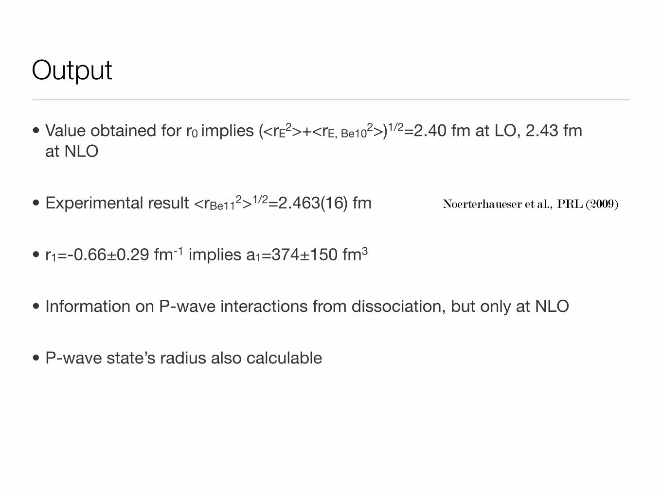
• Value obtained for r0 implies (<rE2>+<rE, Be102>)1/2=2.40 fm at LO, 2.43 fm at NLO

Output
• Value obtained for r0 implies (<rE2>+<rE, Be102>)1/2=2.40 fm at LO, 2.43 fm at NLO
• Experimental result <rBe112>1/2=2.463(16) fm Noerterhaueser et al., PRL (2009)

Output
• Value obtained for r0 implies (<rE2>+<rE, Be102>)1/2=2.40 fm at LO, 2.43 fm at NLO
• Experimental result <rBe112>1/2=2.463(16) fm
• r1=-0.66±0.29 fm-1 implies a1=374±150 fm3
Noerterhaueser et al., PRL (2009)

Output
• Value obtained for r0 implies (<rE2>+<rE, Be102>)1/2=2.40 fm at LO, 2.43 fm at NLO
• Experimental result <rBe112>1/2=2.463(16) fm
• r1=-0.66±0.29 fm-1 implies a1=374±150 fm3
• Information on P-wave interactions from dissociation, but only at NLO
Noerterhaueser et al., PRL (2009)
Output
• Value obtained for r0 implies (<rE2>+<rE, Be102>)1/2=2.40 fm at LO, 2.43 fm at NLO
• Experimental result <rBe112>1/2=2.463(16) fm
• r1=-0.66±0.29 fm-1 implies a1=374±150 fm3
• Information on P-wave interactions from dissociation, but only at NLO
• P-wave state’s radius also calculable
Noerterhaueser et al., PRL (2009)

Output
• Value obtained for r0 implies (<rE2>+<rE, Be102>)1/2=2.40 fm at LO, 2.43 fm at NLO
• Experimental result <rBe112>1/2=2.463(16) fm
• r1=-0.66±0.29 fm-1 implies a1=374±150 fm3
• Information on P-wave interactions from dissociation, but only at NLO
• P-wave state’s radius also calculable
• Universal correlation:
Noerterhaueser et al., PRL (2009)
B(E1) =2e2Q2
c
15π�r2
E�(π)x
�1 + 2x
(1 + x)2
�2
; x = γ1/γ0

Conclusions
Conclusions
• Halo EFT provides a systematic way to organize observables in halo nuclei in an expansion in Rcore/Rhalo

Conclusions
• Halo EFT provides a systematic way to organize observables in halo nuclei in an expansion in Rcore/Rhalo
• Carbon-19: one-neutron halo, shallow S-wave state

Conclusions
• Halo EFT provides a systematic way to organize observables in halo nuclei in an expansion in Rcore/Rhalo
• Carbon-19: one-neutron halo, shallow S-wave state
• Beryllium-11: one-neutron halo, shallow S- and P-wave state

Conclusions
• Halo EFT provides a systematic way to organize observables in halo nuclei in an expansion in Rcore/Rhalo
• Carbon-19: one-neutron halo, shallow S-wave state
• Beryllium-11: one-neutron halo, shallow S- and P-wave state
• 11Be has big B(E1) strength, can be hard to calculate in ab initio methods because of extended nature of p-wave state. Here controlled by r1.
c.f. Rupak & Higa arXiv:1101.0207
Conclusions
• Halo EFT provides a systematic way to organize observables in halo nuclei in an expansion in Rcore/Rhalo
• Carbon-19: one-neutron halo, shallow S-wave state
• Beryllium-11: one-neutron halo, shallow S- and P-wave state
• 11Be has big B(E1) strength, can be hard to calculate in ab initio methods because of extended nature of p-wave state. Here controlled by r1.
• NLO in 11Be: fix A0 from dissociation to continuum, predict radii, extract a1
c.f. Rupak & Higa arXiv:1101.0207

Conclusions
• Halo EFT provides a systematic way to organize observables in halo nuclei in an expansion in Rcore/Rhalo
• Carbon-19: one-neutron halo, shallow S-wave state
• Beryllium-11: one-neutron halo, shallow S- and P-wave state
• 11Be has big B(E1) strength, can be hard to calculate in ab initio methods because of extended nature of p-wave state. Here controlled by r1.
• NLO in 11Be: fix A0 from dissociation to continuum, predict radii, extract a1
• Correlations between low-energy observables
• Other one- (and two-?) neutron (?and proton) halos await: “universality”.
c.f. Rupak & Higa arXiv:1101.0207


