

Endogenous Ranking and Equilibrium Lorenz Curve Across (ex-ante) Identical Countries
By Kiminori Matsuyama1
May 2011
Abstract: This paper considers a model of the world economy with a finite number of ex-ante identical countries and a continuum of tradeable goods, which differ in their dependence on local differentiated producer services. Productivity differences across countries arise endogenously through free entry to the local service sector in each country. In any stable equilibrium, the countries sort themselves into specializing in different sets of tradeable goods and a strict ranking of countries in income, TFP, and the capital-labor ratio emerge endogenously. The equilibrium distribution is characterized by a second-order nonlinear difference equation with two terminal conditions. Furthermore, in the limit as the number of countries increases, the equilibrium Lorenz curve becomes analytically solvable and depends on a few parameters in a tractable manner. This enables us to identify the condition under which the equilibrium distribution obeys a power-law, to show how various forms of globalization affect inequality among countries and to evaluate the welfare effects of trade. Keywords: Endogenous Comparative Advantage, Endogenous Inequality, Globalization and Inequality, Dornbusch-Fischer-Samuelson model, Dixit-Stiglitz model of monopolistic competition, Symmetry-Breaking, Lorenz-dominant shifts, Log-submodularity, Power-law distributions JEL Classification Numbers: F12, F43, O11, O19
1 Email: [email protected]; Homepage: http://faculty.wcas.northwestern.edu/~kmatsu/. Some of the results here have previously been circulated as a memo entitled “Emergent International Economic Order.” I am grateful to conference and seminar participants at Chicago, Harvard, Hitotsubashi, Keio/GSEC, Kyoto, and Princeton for their feedback. I also benefited greatly from the discussion with Hiroshi Matano on the approximation method used in the paper.

©Kiminori Matsuyama, Endogenous Ranking and Equilibrium Lorenz Curve
- 1 -
1. Introduction
This paper considers a model of the world economy with a finite number of (ex-ante)
identical countries. In each country, the representative household supplies a single composite of
primary factors and consumes a continuum of tradeable goods, indexed over the unit interval, as
in the Ricardian model of Dornbusch, Fischer, and Samuelson (1977). Unlike their model,
however, productivity of tradeable goods sectors in each country is endogenous and depends on
the available variety of local differentiated producer services, which is determined by free entry
to the local service sector, as in Dixit and Stiglitz (1977) model of monopolistic competition.
The key assumption is that tradeable goods sectors differ in their dependence on local
differentiated services. This creates a two-way (i.e., reciprocal) causality between patterns of
trade and productivity differences. Having more variety of local services gives a country
comparative advantage in tradeable sectors that are more dependent on those services. This in
turn means a larger market for those services, hence more firms enter to provide such services.
As a result, the country ends up having more variety of local services.
Due to such a circular (or positive feedback) mechanism, any stable equilibrium of the
model has the following features. First, different countries sort themselves into specializing in
different sets of tradeable goods (endogenous comparative advantage). That is, the unit interval
of tradeable goods is partitioned into subintervals such that each country produces and exports
goods in a subinterval. Second, no two countries share the same level of income or TFP. In
other words, a strict ranking of countries in income, TFP, and (in an extension of the model that
allows for variable factor supply) capital-labor ratio emerges endogenously. Third, although the
model is silent about the ranking of each country (because they are ex-ante identical), it
generates a unique distribution across countries (at least with a sufficiently large number of
countries).
More specifically, the equilibrium distribution is fully characterized by a second-order
nonlinear difference equation with two terminal conditions. This equation is not analytically
solvable. However, as the number of countries increases, it becomes analytically solvable and its
unique solution depends on a few parameters in a tractable way. This enables us to study, among
other things, the condition under which the cross-country distribution in income and TFP obeys a
power-law and how various forms of globalization affect inequality across countries, and to
evaluate the welfare effects of trade.

©Kiminori Matsuyama, Endogenous Ranking and Equilibrium Lorenz Curve
- 2 -
For example, the model has a set of parameters that represent the degree of differentiation
across services, the fraction of the consumption goods that are tradeable, and the share of
primary factors of production whose supply can respond to TFP through either factor mobility or
factor accumulation. With these parameters entering the solution in log-submodular way, a
change in these parameters causes a Lorenz-dominant shift of the equilibrium distribution. This
enables us to show that globalization through trade in goods or trade in factors, or skill-biased
technological change that increases the share of human capital and reduces the share of raw
labor, etc., leads to greater inequality among countries. It is also shown that, as the number of
countries increases, the sufficient and necessary condition under which all countries gain from
trade relative to autarky converges to a simple form, which greatly simplifies the task of
evaluating the welfare effects of trade. It is also shown that, when this condition fails, there
exists a set of tradeable goods such that any countries that end up specializing in these goods
would lose from trade. Furthermore, this condition is independent of the degree of
differentiation across services. This means that, as services become more differentiated, the
fraction of countries which end up specializing in these goods increases monotonically and
becomes arbitrarily close to one in the limit where the Dixit-Stiglitz composite of local services
approaches Cobb-Douglas. Thus, perhaps paradoxically, it is possible that almost all countries
may lose from trade under the condition that some countries lose from trade.
Related work: This is a model of symmetry-breaking, a circular mechanism that
generates stable asymmetric equilibria in the symmetric environment due to the instability of the
symmetric equilibrium. The idea that symmetry-breaking creates equilibrium variations across
ex-ante identical countries, groups, regions, or over time has been pursued before.2 Indeed,
symmetry-breaking mechanisms similar to the one used here play a central role in the so-called
new economic geography, e.g., Fujita, Krugman, and Venables (1999) and Combes, Mayer and
Thisse (2008), as well as in international trade, e.g., Krugman and Venables (1995) and
Matsuyama (1996).3 These studies have already shown how inequality among ex-ante identical
2 For a survey on symmetry-breaking in economics, see a New Palgrave entry by Matsuyama (2008), as well as a related entry on “emergence” by Ioannides (2008). 3 See also important precedents by Ethier (1982b) and Helpman (1986, p.344-346), which used external economies of scale to generate the instability of the symmetric equilibrium. The view that trade itself could magnify inequality among nations was discussed informally by Myrdal (1957) and Lewis (1977). See also Williamson (2011) for historical evidence suggesting that great divergence is caused by the first wave of globalization.
©Kiminori Matsuyama, Endogenous Ranking and Equilibrium Lorenz Curve
- 3 -
countries/regions arises, but only within highly simplified frameworks, such as two
countries/regions and/or two tradeable goods. Such a framework may be too stylized and too
restrictive for many empirical researchers working on cross-country variations in income and
TFP. Furthermore, such a stylized framework often comes with highly artificial features.4 The
present model has advantage of allowing for any finite number of countries and generating a
unique equilibrium distribution, which can be approximated by an explicit solution.
Jovanovic (1998, 2009) are perhaps closest in spirit to this paper, although the
mechanisms are quite different. He shows that the steady state distribution of income across (ex-
ante) identical agents emerges and is characterized by a power-law in a model where different
vintages of machines need to be allocated to agents under the restriction that each agent can work
with only one machine or one vintage of machines.5 This induces agents assigned to different
machines to choose different levels of human capital. In Jovanovic (2009), an agent is
interpreted as a country.
More broadly, this paper is also related to other studies, such as Matsuyama (1992),
Acemoglu and Ventura (2002) and Ventura (2005), that point out the need for studying cross-
country income differences in a model of the world economy where interactions across countries
are explicitly spelled out.6
4 Take, for example, Matsuyama (1996), a closest precedent to the present paper. It assumes, for the sake of the tractability, two tradeable goods and a continuum of ex-ante identical countries, and shows that there is a continuum of equilibrium distributions, all of which have two clusters of countries. While it achieves the goal of showing how inequality arises among ex-ante identical countries, the prediction that there is a continuum of equilibrium distributions is an artifact of the assumption that there is a continuum of countries and the prediction of two clusters of countries is an artifact of the assumption that there are only two tradeable goods. 5 As Jovanovic (2009, p.711) pointed out, this restriction plays a crucial role in generating inequality in his model. Without it, all agents would be assigned to the same set of machines and remain identical. 6 As a theory of endogenous inequality of nations, the symmetry-breaking approach may be contrasted with an alternative, which may be called the “poverty trap” or “coordination failure” approach. Consider any model of poverty traps that analyzes a country in isolation, either as a closed economy or as a small open economy, such as Murphy, Shleifer and Vishny (1989), Matsuyama (1991), Ciccone and Matsuyama (1996), and Rodríguez (1996). These studies show how some strategic complementarities create multiple equilibria (in static models) or multiple steady states (in dynamic models). It has been argued that such a model may explain diverse economic performance across inherently identical countries, simply because different equilibria (or steady states) may prevail in different countries. In other words, some countries suffer from coordination failures, locked into poverty traps, while others do not. Although the poverty trap approach suggests the possibility of co-existence of the rich and the poor, it does not suggest that such co-existence is the only stable patterns. The symmetric patterns are also stable. Without the broken symmetry, this approach cannot yield any prediction regarding the effects of globalization on the degree of the inequality among nations. Moreover, the two approaches have different policy implications. According to the poverty trap approach, the case of underdevelopment is an isolated problem, which can be treated independently for each country. According to the symmetry-breaking approach, it is a part of the interrelated whole, and needs to be dealt with at the global level. Matsuyama (2002) discusses the differences between the two approaches in more detail.
©Kiminori Matsuyama, Endogenous Ranking and Equilibrium Lorenz Curve
- 4 -
A Technical Remark: As described above, we derive the equilibrium condition for a
finite number of countries and a continuum of goods, which is not analytically solvable. Then,
we let the number of countries go to infinity to solve it analytically. Some readers might wonder
why we do not assume a continuum of countries and a continuum of goods from the very
beginning. Indeed, the assumption that countries are outnumbered by goods plays an essential
role in the following analysis. Countries that are ex-ante identical become ex-post heterogeneous
in the model only by sorting themselves into producing different sets of goods. For example,
suppose that there were more countries than goods. In such a setup, it would not be possible for
different countries to specialize in different sets of goods, so that some countries would remain
identical ex-post, which means that there would be no strict ranking of countries. If the number
of goods were equal to the number of countries (as in the two-country two-sector models cited
above), then a strict ranking could emerge, but only under some additional parameter restrictions.
By adding more goods while keeping the number of countries constant, the parameter restrictions
would become less stringent, but they would never go away. However, with a continuum of
goods, there is enough room for a finite number of countries to sort themselves so that the
equilibrium is always characterized by a strict ranking, without any additional parameter
restrictions. Furthermore, the property of a strict ranking remains intact even as the number of
countries goes to infinity. This is because the countries are, being at most countably many, still
grossly outnumbered by a continuum of goods. In other words, by assuming a finite number of
countries in a world with a continuum of goods, and by letting the number of countries go to
infinity, we are able to keep the situation where the goods grossly outnumber the countries, and
at the same time, to eliminate the integer constraint on countries to solve the equilibrium
distribution analytically.7
7 Of course, there are some models where the equilibrium is characterized by a mapping between two sets of continuum. However, they usually deal with the situation where an exogenous ordering is given in each set. For example, Costinot and Vogel (2010) consider a matching between a continuum of ex-ante heterogeneous factors and a continuum of ex-ante heterogeneous goods each of which is given an exogenous ordering. Or they have additional restrictions on matching. For example, in Jovanovic (1998, 2009), a continuum of ex-ante identical agents is matched with a continuum of heterogeneous technologies, under the assumption that each agent can be assigned to only one technology. In the present setup, there is no compelling reason to impose such a restriction. In fact, each country is matched to produce a continuum of goods, even in the limit where countries are countably many.
©Kiminori Matsuyama, Endogenous Ranking and Equilibrium Lorenz Curve
- 5 -
The rest of the paper is organized as follows. Section 2 studies the basic model, which
assumes that all consumption goods are tradeable and all primary factors are in fixed supply.
After the key elements of the model are laid out in section 2.1, the unique equilibrium in a
single-country world, which may be also viewed as an autarky equilibrium, is derived in section
2.2. Section 2.3 looks at the two-country case, and shows that a symmetric pair of asymmetric
stable equilibria emerges via symmetry-breaking. Section 2.4 generalizes this to any finite
number of countries. It shows the emergence of an endogenous ranking across a finite number
of countries, and derives the difference equation that characterizes the distribution. Section 2.5
studies the limit case, where the number of countries goes to infinity. To the best of my
knowledge, the method used to derive the limit solution is new in economics and might be of
independent interest. With the analytical solution for the equilibrium distribution in hand, this
subsection then looks at power-law examples, and shows that, when a smaller share of the
consumer expenditure goes to the sectors that use local services more intensively, the distribution
drops more sharply in the upper end, as a smaller fraction of countries specialize in producing
such goods. This subsection also shows how log-submodularity helps to prove that a change in
the degree of differentiation causes a Lorenz-dominant shift. Section 2.6 conducts the welfare
analysis. Section 3 offers two extensions of the basic model. In section 3.1, a fraction of the
consumption goods are assumed to be nontradeable. By reducing this fraction, which enters the
solution in a log-submodular way, the extension allows us to show how globalization through
trade in goods causes a Lorenz-dominant shift, leading to a greater inequality across countries.
In section 3.2, one of the primary factors is allowed to vary in supply either through factor
mobility and factor accumulation. Again, the share of this factor in production enters the
solution in a log-submodular way, which allows us to show that technological change that
increases the relative importance of human capital in production and of globalization through
trade in factors causes Lorenz-dominant shifts, leading to a greater inequality. Section 4
concludes.
2. Basic Model:
2.1 Key Elements of the Model
The world consists of J (ex-ante) identical countries, where J is a positive integer. There
may be multiple nontradeable primary factors of production, such as capital (K), labor (L), etc.,

©Kiminori Matsuyama, Endogenous Ranking and Equilibrium Lorenz Curve
- 6 -
but they can be aggregated to a single composite as V = F(K, L, …). For now, it is assumed that
these factors are in fixed supply and that the representative consumer of each country is endowed
with the same quantity of the (composite) primary factor, V. (Later, one of the component
factors is allowed to vary in supply across countries endogenously through factor mobility or
factor accumulation.)
As in Dornbusch, Fischer and Samuelson (1977), the representative consumer has Cobb-
Douglas preferences over a continuum of tradeable consumption goods, indexed by s [0,1].
This can be expressed by an expenditure function, UdssPsE
1
0))(log()(exp =
UsdBsP
1
0)())(log(exp , where U is utility, P(s) > 0 the price of good-s, and
sduusB
0)()(
the expenditure share of goods in [0,s], satisfying )()(' ssB > 0, 0)0( B , and 1)1( B . By
denoting the aggregate income by Y, the budget constraint is then written as
(1) UdssPsY
1
0))(log()(exp UsdBsP
1
0)())(log(exp .
The assumption of Cobb-Douglas preferences not only helps to keep the algebra simple but also
implies that each good is produced somewhere in the world, which plays an important role in the
ensuing analysis.
Each tradeable consumption good is produced competitively with constant returns to
scale technology, using nontradeable inputs. They are the (composite) primary factor of
production as well as a composite of differentiated local producer services, aggregated by a
symmetric CES, as in Dixit and Stiglitz (1977). The primary factor and the composite of local
producer services are combined with a Cobb-Douglas technology with γ(s) [0,1] being the
share of local producer services in sector-s. The unit cost of production in each tradeable goods
sector can thus be expressed as
(2) )(
0
1)(11)(
0
1)(1 )())(()())(()(sns
sns dzzpsdzzpssC
,
with
111
01
1
,
where ω is the price of the (composite) primary factor; n the range of differentiated producer
services available in equilibrium; p(z) the price of a variety z [0,n]. The parameter, σ > 1, is

©Kiminori Matsuyama, Endogenous Ranking and Equilibrium Lorenz Curve
- 7 -
the direct partial elasticity of substitution between every pair of local services. It turns out to be
notationally more convenient to define 0)1/(1 , which I shall call the degree of
differentiation. What is crucial here is that the tradeable sectors differ in their dependence on the
differentiated local services, γ(s). With no loss of generality, we may order the tradeable goods
such that γ(s) is weakly increasing. For technical reasons, we also assume that γ(s) is strictly
increasing and continuously differentiable in s [0,1].
Monopolistic competition prevails in the local services sector. Each variety is supplied
by a single firm, which uses T(q) = f +mq units of the primary factor to supply q units so that the
total cost is ω(f +mq), of which the fixed cost is ωf and ωm represents the marginal cost. As is
well-known, each monopolistically competitive firm would set its price equal to p(z) = (1+θ)ωm
in the standard Dixit-Stiglitz environment. This would mean that it might not be clear whether
the effects of shifting 0)1/(1 should be attributed to a change in the degree of
differentiation or a change in the mark-up rate. To separate these two conceptually, I depart
from the standard Dixit-Stiglitz specification by introducing a competitive fringe. That is, once a
firm pays the fixed cost of supplying a particular variety, any other firms in the same country
could supply its perfect substitute with the marginal cost equal to (1+ν)ωm > ωm without paying
any fixed cost, where ν > 0 is the productivity disadvantage of the competitive fringe. When
, the presence of such competitive fringe forces the monopolistically competitive firm to
charge a limit price,
(3) p(z) = (1+ ν)ωm, where 0 .
Note that this pricing rule generalizes the standard Dixit-Stiglitz formulation, as the latter is
captured by the special case, . This generalization is introduced merely to demonstrate that
the main results are independent of ν, when , so that the effects of θ should be interpreted
as those of changing the degree of differentiation, not the mark-up rate.8
From (3), the unit cost of production in each tradeable sector, given by (2), is simplified
to:
(4)
)()(
)(
0
1)(1 )()1()()())(()( ss
sns nmsdzzpssC
.
8 This generalization of the Dixit-Stiglitz monopolistic competition model to separate the roles of mark-ups and product differentiation has been used previously by, e.g. Matsuyama and Takahashi (1998) and Acemoglu (2009, Ch.12.4.4). Murphy, Shleifer, and Vishny (1989), Grossman and Helpman (1991) and Matsuyama (1995) also used the limit pricing for related monopolistic competition models.
©Kiminori Matsuyama, Endogenous Ranking and Equilibrium Lorenz Curve
- 8 -
Note that, given ω, a higher n reduces the unit cost of production in all tradeable sectors, which
is nothing but productivity gains from variety, as discussed by Ethier (1982a) and Romer (1987).
Eq. (4) shows that this effect is stronger for a larger θ, and that higher-indexed sectors gain more
from such variety effect, which plays an important role in the ensuing analysis.
Since all the services are priced equally and enter symmetrically into the production
functions, q(z) = q for all z [0,n]. This implies that the profit of all service providers is given
by π(z) = pq − ω(mq + f) = ω(vmq − f) for all z [0,n], from which each service provider earns
zero profit if and only if:
(5) vmq = f.
Free entry to (or free exit from) the local producer services sector ensures that eq.(5) holds in
equilibrium.
Before proceeding, we may set,
(6) β(s) = 1 for all s [0,1],
so that B(s) = s for all s [0,1] by choosing the tradeable goods indices, without any further loss
of generality.9 In words, we measure the size of (a set of ) sectors by the expenditure share of the
goods produced in these sectors. With this indexing, the size of sectors whose γ is less than or
equal to γ(s) is equal to s. It also means that a country’s share in the world income is equal to the
measure of the tradeable sectors for which the country ends up having comparative advantage in
equilibrium, as will be shown.
2.2 Single-Country (or Autarky) Equilibrium (J = 1)
First, let us look at the equilibrium allocation for J = 1. This can be viewed as the case of
a one-country world. Alternatively, this can also be viewed as the equilibrium allocation of each
country in autarky, which would serve as the benchmark for evaluating the welfare effects of
trade in the world economy with multiple countries.
9 To see this, starting from any indexing of the goods s' [0,1] satisfying i) )'(~ s is strictly increasing in s' [0,1],
ii) )'(~ s > 0 for all s' [0,1], and iii) 1')'(~1
0 dss , re-index the goods by a monotone increasing transformation,
'
0)(~)'(~ sduusBs . Then, ))(~(~)( 1 sBs is strictly increasing in s [0,1], and ')'(~ dssds , hence β(s) = 1
for all s [0,1].

©Kiminori Matsuyama, Endogenous Ranking and Equilibrium Lorenz Curve
- 9 -
Because of Cobb-Douglas preferences, all the consumption goods must be consumed by
positive amounts. Hence, in the absence of trade, the economy must produce all the
consumption goods, which means that their prices must be equal to their costs; that is,
(7) )()( )()1()()()( ss nmssCsP for all s [0,1]
Since the representative consumer spends β(s)Y = Y on good-s, and sector-s spends 100γ(s)% of
its revenue on producer services, the total revenue of the producer services sector is
(8) npq = n(1+ν)mωq = 1
0
)()( Ydsss = A Y,
where
(9) 1
0
)( dssA .10
Thus, in autarky, the share of the producer services sector in the aggregate income is equal to the
average share of the producer services across all the consumption goods sectors. (Here,
superscript A stands either for Autarky or for Average).
Likewise, sector-s spends 100(1−γ(s))% of its revenue on the primary factor.
Furthermore, each service provider spends ω(f+mq) on the primary factor. Therefore, the total
income earned by the (composite) primary factor is equal to:
(10) ωV = 1
0
)())(1( Ydsss + nω(f+mq) = (1−Γ A)Y + nω(f+mq);
Combining (8) and (10) yields
nfVYA
/11/11 ;
f
nVmq A
A
/11,
to which we insert the free-entry condition (5) to determine the variety of differentiated services
(and the number of service providers) as well as the aggregate income as follows:
(11)
f
Vn AA
1
10 It might be useful to explain how the re-indexation discussed in the previous footnote works here. Under a
general indexing, 1
0')'(
~)'(~ dsssA . With the re-indexing,
'
0)(~)'(~ sduusBs , this can be rewritten as
1
0
1
0
1 )())(~(~ dssdssBA .

©Kiminori Matsuyama, Endogenous Ranking and Equilibrium Lorenz Curve
- 10 -
(12) YA = ωAV = ωAF(K,L,…).
Two points about the above equilibrium deserves emphasis. First, as shown in eq. (11),
the equilibrium variety of producer services, nA, is proportional to the share of producer services
in the total expenditure, which is equal to A in autarky. Second, free entry ensures zero profit,
so that the aggregate income of the economy is accrued entirely to the primary factors, as shown
in eq.(12). Because all the primary factors, capital (K), labor (L), etc. can be aggregated into a
single composite, V =F(K,L,…), the equilibrium price of the composite factor is nothing but the
total factor productivity (TFP) as is commonly measured in GDP accounting exercises.
2.3 Two-Country Equilibrium (J = 2)
Let us now turn to the trade equilibrium with two ex-ante identical countries, Home and
Foreign. Since they are ex-ante identical, they share the same values for all the exogenous
parameters. However, endogenous variables, such as n and ω, might take (and in fact will be
shown to take) different values, so that asterisks (*) are used to denote Foreign values to
distinguish them from Home values.
From (4), the relative cost of production in sector-s is given by:
*
)(
** )()(
s
nn
sCsC ,
which is increasing in s if n < n*; decreasing in s if n > n*; and independent of s if n = n*. This
shows the patterns of comparative advantage. The country with a more developed local support
industry has comparative advantage in higher-indexed sectors, which rely more heavily on local
producer services. However, unlike the standard neoclassical theory of trade, the source of
comparative advantage is endogenous here because n and n* are endogenous.
To solve for an equilibrium allocation, suppose n < n* for the moment, hence the graph of
C(s)/C*(s) is upward-sloping, as shown in Figure 1. The height of this graph depends on ω/ω*,
the relative factor prices. If ω/ω* were so high to make the graph of C(s)/C*(s) lie everywhere
above one, Home would import all the goods from Foreign, while exporting none; this cannot be
an equilibrium. Similarly, ω/ω* cannot be so low to make the graph of C(s)/C*(s) lie
everywhere below one. Thus, in equilibrium, Home produces and exports s [0, S) & Foreign
produces and exports s (S, 1], where S (0, 1) is defined by

©Kiminori Matsuyama, Endogenous Ranking and Equilibrium Lorenz Curve
- 11 -
1)()(
*
)(
**
S
nn
SCSC ,
as shown in Figure 1.11 This means that the equilibrium factor prices can be expressed as
(13) 1)(
**
S
nn
.
Thus, due to the productivity effect of more variety (n < n*), the factor price is higher at Foreign
than at Home (ω < ω*).
Because of Cobb-Douglas preferences, the total revenue of Home sector-s [0, S) is
equal to β(s)(Y+Y*) = Y+Y*, of which 100γ(s)% goes to the Home producer services. Thus, by
adding up across all sectors in [0, S), the total revenue of the Home producer services sector is
(14) npq = n(1+ν)mωq =
S
dss0
)( (Y+Y*) = Γ−(S)S(Y+Y*),
where
(15) S
dssS
S0
)(1)( ,
is the average share of producer services across all tradeable sectors in [0, S). Clearly, it is
increasing in S so that AS )1()()0()0( .
Likewise, for each s [0, S), Home sector-s spends 100(1−γ(s))% of its revenue on the
Home primary factor. Furthermore, each Home service provider spends ω(f+mq) on the Home
primary factor. Therefore, the total income earned by the Home (composite) primary factor is
equal to:
(16) ωV = (1− Γ–(S))S(Y+Y*)+ nω(mq +f)
Combining (14) and (16) yields
nfVS
YYS
)(/11
/11)( *
;
fnV
SSmq
)(/11)(
,
to which we insert the free entry condition (5) to obtain:
(17)
fVSn
1)( ;
11 The borderline sector, S, can be produced in either country and its trade flow is indeterminate. This type of indeterminacy is inconsequential, and hence ignored in the following discussion.

©Kiminori Matsuyama, Endogenous Ranking and Equilibrium Lorenz Curve
- 12 -
(18) ...),()( * LKFVYYSY .
Thus, the equilibrium variety of Home local services is proportional to AS )( ; S represents
Home’s share in the world income and ω Home’s TFP.
Likewise, one could follow the same steps for Foreign sector-s (S, 1] to obtain
(19)
fVSn
1)(* ;
(20) ...),())(1( **** LKFVYYSY .
where
(21)
1
)(1
1)(S
sS
S .
is the average share of producer services across all the tradeable sectors in (S, 1], which is
increasing in S so that with )1()1()()0( SA . In particular, for any S (0, 1),
)()( SS A ,
which in turn implies, from (11), (17) and (19), n < nA < n*. Thus, our initial supposition that n
< n* hold in equilibrium has now been verified. Furthermore, from (18) and (20),
(22) 11**
S
SYY
so that the distribution is fully characterized by S, which, from (13) and (22) satisfies
(23) 1)()(
1
)(
S
SS
SS
.
In summary, this demonstrates the existence of an equilibrium, where Home produces and
exports s [0, S) and Foreign produces and exports s (S, 1], where S, determined by eq. (23),
represents the Home share in both income and TFP.
Recall that we began the analysis by supposing n < n* to obtain the above equilibrium.
By supposing n > n* instead, we can obtain another equilibrium, which is the mirror-image of
the above equilibrium, where the positions of the two countries are reversed.
The intuition behind the existence of such a symmetric pair of asymmetric equilibriums is
a two-way causality between the patterns of trade and comparative advantage. A country with a
more developed local services sector has comparative advantage in tradeable sectors that depend
more on local services. And a country with a comparative advantage in those sectors has a more

©Kiminori Matsuyama, Endogenous Ranking and Equilibrium Lorenz Curve
- 13 -
developed local services sector. Since these two equilibriums are the mirror-images of each
other; they both predict the same equilibrium distribution of income and of TFP in the world
economy, summarized by S, a solution to eq. (23).12
Indeed, there is another equilibrium, where n = n* = nA. In this symmetric equilibrium,
which replicates the autarky equilibrium in each country, the unit cost of production of each
tradeable good is equal across two countries, so that the consumers everywhere is indifferent as
to which country they purchase tradeable goods from. In other words, the patterns of trade are
indeterminate in this case. If exactly 50% of the world income is spent on each country’s
tradeable goods sectors, and if this spending is distributed across the two countries in such a way
that the local services sector of each country ends up receiving exactly 2/A fraction of the
world spending, then free entry to this sector in each country would lead to n = n* = nA.
However, it is easy to see that this equilibrium is fragile in that the required spending patterns
described above must be exactly met in spite that the consumers are indifferent. Furthermore,
this equilibria is unstable in that a small perturbation that causes n > n* (n < n*) would lead to
an abrupt change in the spending patterns that makes the profit of Home local service firms rise
(fall) discontinuously, which leads to a higher (lower) n and the profit of Foreign local service
firms fall (rise) discontinuously, which leads to a lower (higher) n*.
The mechanism that causes the instability of the symmetric equilibrium, n = n* = nA, is
indeed the same two-way causality that generates the symmetric pair of stable asymmetric
equilibriums demonstrated above. Although such a symmetry-breaking mechanism is well-
known in the literature on international trade and economic geography, they are usually
demonstrated in models of two countries or regions. One of the advantages of the present model
is that it can be extended to any finite number of countries.
2.4 Multi-Country Equilibrium (2 < J < ∞)
Note first that the same logic behind the instability of the symmetric equilibrium in the
two-country world implies that no two countries share the same value of n in any stable
equilibrium. The countries can be thus ranked in such a way that Jjjn
1is a monotone
12 Although I have been unable to find an example, eq.(23) might have multiple solutions for some γ functions. If this is the case, there is a symmetric pair of asymmetric stable equilibria for each solution to eq. (23). However, I am not concerned about the possibility of this kind of multiplicity, as it can be ruled out for a sufficiently large J, as will be seen below.
©Kiminori Matsuyama, Endogenous Ranking and Equilibrium Lorenz Curve
- 14 -
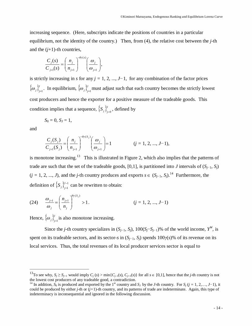
increasing sequence. (Here, subscripts indicate the positions of countries in a particular
equilibrium, not the identity of the country.) Then, from (4), the relative cost between the j-th
and the (j+1)-th countries,
1
)(
11 )()(
j
j
s
j
j
j
j
nn
sCsC
,
is strictly increasing in s for any j = 1, 2, ..., J−1, for any combination of the factor prices
Jjj 1
. In equilibrium, Jjj 1
must adjust such that each country becomes the strictly lowest
cost producers and hence the exporter for a positive measure of the tradeable goods. This
condition implies that a sequence, JjjS
0, defined by
S0 = 0, SJ = 1,
and
1)(
)(
1
)(
11
j
j
S
j
j
jj
jjj
nn
SCSC
(j = 1, 2, ..., J−1),
is monotone increasing.13 This is illustrated in Figure 2, which also implies that the patterns of
trade are such that the set of the tradeable goods, [0,1], is partitioned into J intervals of (Sj−1, Sj)
(j = 1, 2, ..., J), and the j-th country produces and exports s (Sj−1, Sj).14 Furthermore, the
definition of 1
1
JjjS can be rewritten to obtain:
(24) 1)(
11
jS
j
j
j
j
nn
. (j = 1, 2, ..., J−1)
Hence, Jjj 1
is also monotone increasing.
Since the j-th country specializes in (Sj−1, Sj), 100(Sj−Sj−1)% of the world income, YW, is
spent on its tradeable sectors, and its sector-s in (Sj−1, Sj) spends 100γ(s)% of its revenue on its
local services. Thus, the total revenues of its local producer services sector is equal to
13To see why, Sj ≥ Sj+1 would imply Cj (s) > min{Cj–1(s), Cj+1(s)} for all s [0,1], hence that the j-th country is not the lowest cost producers of any tradeable good, a contradiction. 14 In addition, S0 is produced and exported by the 1st country and SJ by the J-th country. For Sj (j = 1, 2,…, J−1), it could be produced by either j-th or (j+1)-th country, and its patterns of trade are indeterminate. Again, this type of indeterminacy is inconsequential and ignored in the following discussion.
©Kiminori Matsuyama, Endogenous Ranking and Equilibrium Lorenz Curve
- 15 -
(25) njpjqj = nj(1+ν)mωjqj =
j
j
S
S
dss1
)( YW = (Sj−Sj−1)ГjYW, (j = 1, 2, ...,J )
where
(26)
j
j
S
Sjjjjj dss
SSSS
1
)(1),(1
1 . (j = 1, 2, ...,J )
is the average share of producer services across all tradeable sectors in (Sj−1, Sj). Since )( is
increasing, Jjj 1
is also monotone increasing.
Likewise, in the j-th country, sector-s (Sj−1, Sj) spends 100(1−γ(s))% of its revenue on
its primary factor, and each service provider spends ωj(f+mqj) on its primary factor. Thus, the
total income earned by the primary factor in the j-th country is equal to:
(27) ωjV = (1− Гj)(Sj−Sj−1)YW + njωj(mqj + f) (j = 1, 2, ...,J )
Combining (25) and (27) yields:
fnVYSS
jjj
Wjj
/11/11)( 1 ;
f
nVmq
jj
jj
/11
(j = 1, 2, ...,J )
to which we insert the free-entry, zero profit condition (5) to yield
(28)
f
Vn jj
1; (j = 1, 2, ...,J )
and
(29) Wjjjj YSSVY )( 1 . (j = 1, 2, ...,J )
Because Jjj 1
is monotone increasing, eq.(28) shows that Jjjn
1is also monotone increasing, as
has been assumed. Eq.(29) shows that j represents TFP of the j-th poorest country, and
1 jjj SSs , the measure of the tradeable goods in which this country has comparative
advantage, is also equal to its share in the world income. It also implies that
j
k kj sS1
represents the cumulative share of the j poorest countries in the world income.
Finally, by combining (24), (28), and (29), we obtain the equation that determines JjjS
0
that characterizes the distribution of income (as well as of TFPs) across countries:

©Kiminori Matsuyama, Endogenous Ranking and Equilibrium Lorenz Curve
- 16 -
(30) 1),(),(
)(
1
1
1
1
jS
jj
jj
jj
jj
SSSS
SSSS
with 00 S and 1JS .
To summarize;
Proposition 1: Let jS be the cumulative share of the j poorest countries in the world income.
Then, JjjS
0 is a solution to the nonlinear 2nd-order difference equation with two terminal
conditions:
(30) 1),(),(
)(
1
1
1
1
jS
jj
jj
jj
jj
SSSS
SSSS
with 00 S & 1JS ,
where
j
j
S
Sjjjj dss
SSSS
1
)(1),(1
1 .
Figure 3 illustrates a solution to eq.(30) graphically by means of the Lorenz curve,
]1,0[]1,0[: J , defined by the piece-wise linear function, satisfying jJ SJj )/( . From this
Lorenz curve, we can easily recover Jjjs
0, the distribution of the country shares in the world
income and vice versa.15 A few points deserve emphasis. First, because ),( 1 jj SS is increasing
in j, jj ss /1 /)( 1 jj SS )( 1 jj SS is increasing in j. Hence, the Lorenz curve is kinked at Jj /
for each j = 1, 2, ..., J−1. In other words, the ranking of the countries is strict.16 Second, since
both income and TFP are proportional to 1 jjj SSs , the Lorenz curve here also represents the
Lorenz curve for income and TFP. Third, we could also obtain the ranking of countries in other
variables of interest that are functions of Jjjs
0. For example, the j-th country’s share in world
trade can be shown to be equal to
J
k kkjj ssss1
22 / , which is increasing in j . The j-th
15 This merely states that there is a one-to-one correspondence between the distribution of income and the Lorenz curve. With J ex-ante identical countries, there are J! (factorial) equilibria for each Lorenz curve. Furthermore, there may be multiple solutions to (30), although such multiplicity can be ruled out for a sufficiently large J, as will be seen below. 16 This is in sharp contract to the model of Matsuyama (1996), which generates a non-degenerate distribution of income across countries, but with a clustering of countries that share the same level of income. The crucial difference is that the countries outnumber the tradeable goods in the model of Matsuyama (1996), while the tradeable goods outnumber the countries in the present model.
©Kiminori Matsuyama, Endogenous Ranking and Equilibrium Lorenz Curve
- 17 -
country’s trade dependence, defined by the volume of trade divided by its GDP, can be shown to
be equal to js1 , which is decreasing in j.
Even though the nonlinear difference equation, eq. (30), fully characterizes the
equilibrium distribution across countries, it is not analytically solvable. Of course, one could try
to solve it numerically. However, numerical methods are not useful for answering the question
of the uniqueness or for determining how the solution depends on the parameters of the model.
Instead, in spirit similar to the central limit theorem, let us approximate the equilibrium Lorenz
curve by J
Jlim . It turns out that, as J ∞, eq.(30) converges to the nonlinear 2nd-
order differential equation with a unique solution that can be solved analytically. This allows us
to study not only the effects of changing the parameters on the Lorenz curve, but also the welfare
effects of trade.
2.5 Equilibrium Lorenz Curve: Limit Case (J ∞)
I will now sketch the method to obtain the limit Lorenz curve, J
Jlim . Although
the method is technical in nature, it is worthwhile partly because the method will be used again
in extensions of the model, and partly because it might be potentially useful for other
applications in economics. The basic strategy is to take Taylor expansions on both sides of eq.
(30).17
First, by setting Jjx / and Jx /1 ,
221
2
)(")(')()( xoxxxxxxSS xjj
,
221
2
)(")(')()( xoxxxxxxSS xjj ,
from which the LHS of eq. (30) can be written as:
xoxxx
SSSS
jj
jj
)(')("1
1
1 .
Likewise,
)()('))(('21))((
)()(
)(),(
)(
)(1 xoxxxx
xxx
dssSS
xx
xjj
17 Initially, I obtained the limit by a different method, which involves repeated use of the mean value theorem. I am grateful to Hiroshi Matano for showing me this (more efficient) method.

©Kiminori Matsuyama, Endogenous Ranking and Equilibrium Lorenz Curve
- 18 -
)()('))(('21))((
)()(
)(),(
)(
)(1 xoxxxx
xxx
dssSS
x
xxjj
from which the RHS of eq.(30) can be written as:
))(()(
1
1 )('))(())(('1
),(),( xS
jj
jj xoxxxx
SSSS j
xoxxx )('))(('1 .
By combining these, eq.(30) becomes:
xoxxxxoxxx
)('))(('1)(')("1 .
By letting 0/1 Jx , eq.(30) becomes:
(31) )('))((')(')(" xx
xx
.
To solve it, integrate it once to obtain
0))(()('log cxx or 0)('))((exp cexx
where c0 is a constant to be determined. By integrating the above once again,
xecdse cx
s 01
)(
0
)(
,
where c1 is another constant to be determined. From the two terminal conditions, 0)0( and
1)1( ,
00
0
)(1 dsec s ;
1
0
)(0 dsee sc ;
from which the solution, ]1,0[]1,0[: , is determined uniquely by
xduedse ux
s
1
0
)()(
0
)( ,
which can be rewritten more compactly as:
(32)
)(
0
)()(x
dsshxHx , where
1
0
)(
)(
)(due
eshu
s
.

©Kiminori Matsuyama, Endogenous Ranking and Equilibrium Lorenz Curve
- 19 -
To summarize:
Proposition 2: The limit equilibrium Lorenz curve, JJ lim = , is characterized by the
nonlinear 2nd-order differential equation with the two terminal conditions:
(31) )('))((')(')(" xx
xx
with 0)0( and 1)1(
whose unique solution is given by:
(32)
)(
0
)()(x
dsshxHx , where
1
0
)(
)(
)(due
eshu
s
.
Figure 4 illustrates the unique solution, (32). As shown in the left panel, )(sh is positive and
decreasing in s [0, 1]. Thus, its integral, )(sHx , is increasing and concave. Furthermore,
)(sh is normalized in such a way that 0)0( H and 1)1( H , as shown in the right panel.
Hence, its inverse function, the Lorenz curve, xHxs 1)( is increasing, convex, with
0)0( and 1)1( .
It is also worth noting that the limit Lorenz curve, )(xs , may be viewed as the one-to-
one mapping between a set of countries (on the x-axis) and a set of the goods they produce (on
the s-axis).
With the limit Lorenz curve xHxs 1)( in hand, one could easily calculate:
Share of Country at 100x% in World GDP: dxedsedxx xs ))((1
0
)()('
.
GDP of Country at 100x% (with World GDP normalized to one):
))((1
0
)()(' xs edsexy
Ratio of the richest to the poorest: eehh
HH
yy
Min
Max
))0(1(
)1()0(
)1(')0('
)0(')1(' .
Furthermore, the cumulative distribution function (cdf) of (normalized) GDPs, y, can be readily
calculated as )()'()( 1 yyx . Table illustrates such calculation by using power-law (e.g.,
truncated Pareto) examples.

©Kiminori Matsuyama, Endogenous Ranking and Equilibrium Lorenz Curve
- 20 -
Table: Power-Law Examples Example 1:
ss )( Example 2:
1
)1(1log)( ses
Example 3:
1
)1(1log)( ses ; );0( Inverse Lorenz Curve
)(sHx
ee s
11
1
)1(1log se 1
1)1(11
ese
Lorenz Curve: )(xs )(1 xH
1
)1(1log xe
11
ee x
1
1)1(1
exe
Cdf: )(yx
)()'( 1 y ye 1
11
ye
1log1
ey
y
ey
yMaxMin
1
11
1
111
Pdf: )(y )(' y 2
1y
y1 2
1)/(1)/( )()()(
1)/(
y
yy MinMax
Support ],[ MaxMin yy ye
1
1
e 11
eey
e ye
e
1
1
ee
e
11
In this table, Example 1 and Example 2 may be viewed as the limit cases of Example 3, as
0 and , respectively. Note that, as varies from −∞ to +∞, the “power” in the
probability density function (pdf), 2/ , changes from −∞ to +∞. As → −∞, a smaller
fraction of the consumer expenditure goes to the sectors that use local services more intensively.
This means that just a small fraction of countries specialize in such “desirable” tradeable goods.
As a result, the pdf declines more sharply in the upper end.
Another advantage of the limit Lorenz curve, (32), is that one could easily see the effect
of changing θ, which is illustrated in Figure 4. To see this, note first that )()(ˆ sesh , the
numerator of )(sh , satisfies
0)('))(ˆlog(2
ss
sh
.
In words, it is log-submodular in θ and s.18 Thus, a higher θ shifts the graph of )()(ˆ sesh
down everywhere but proportionately more at a higher s. Since )(sh is a rescaled version of
)(ˆ sh to keep the area under the graph unchanged, the graph of )(sh is rotated “clockwise” by a
18See Topkis (1998) for mathematics of super- and sub-modularity and Costinot (2009) for a recent application to international trade.
©Kiminori Matsuyama, Endogenous Ranking and Equilibrium Lorenz Curve
- 21 -
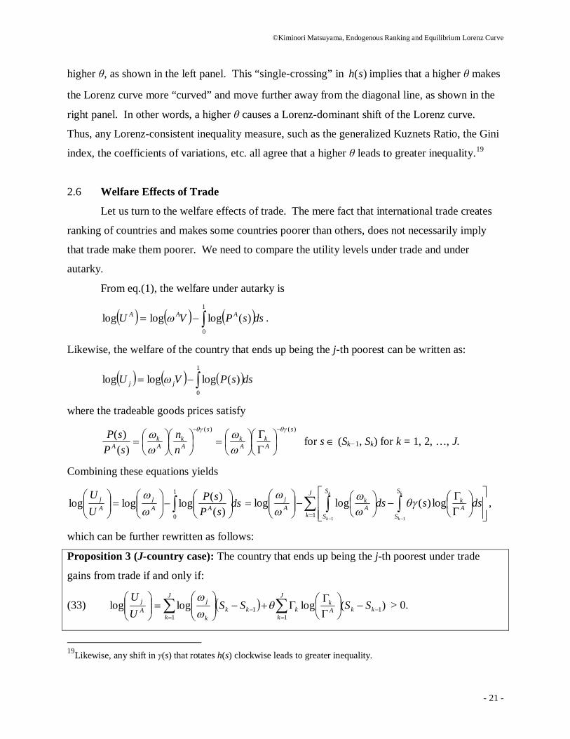
higher θ, as shown in the left panel. This “single-crossing” in )(sh implies that a higher θ makes
the Lorenz curve more “curved” and move further away from the diagonal line, as shown in the
right panel. In other words, a higher θ causes a Lorenz-dominant shift of the Lorenz curve.
Thus, any Lorenz-consistent inequality measure, such as the generalized Kuznets Ratio, the Gini
index, the coefficients of variations, etc. all agree that a higher θ leads to greater inequality.19
2.6 Welfare Effects of Trade
Let us turn to the welfare effects of trade. The mere fact that international trade creates
ranking of countries and makes some countries poorer than others, does not necessarily imply
that trade make them poorer. We need to compare the utility levels under trade and under
autarky.
From eq.(1), the welfare under autarky is
dssPVU AAA 1
0
)(logloglog .
Likewise, the welfare of the country that ends up being the j-th poorest can be written as:
dssPVU jj 1
0
)(logloglog
where the tradeable goods prices satisfy
)()(
)()( s
Ak
Ak
s
Ak
Ak
A nn
sPsP
for s (Sk−1, Sk) for k = 1, 2, …, J.
Combining these equations yields
dssP
sPUU
AAj
Aj
1
0 )()(logloglog
J
k
S
SAk
S
SAk
Aj
k
k
k
k
dssds1 11
log)(loglog
,
which can be further rewritten as follows:
Proposition 3 (J-country case): The country that ends up being the j-th poorest under trade
gains from trade if and only if:
(33)
Aj
UU
log
J
kkkA
kk
J
kkk
k
j SSSS1
11
1 )(loglog
> 0.
19Likewise, any shift in γ(s) that rotates h(s) clockwise leads to greater inequality.
©Kiminori Matsuyama, Endogenous Ranking and Equilibrium Lorenz Curve
- 22 -
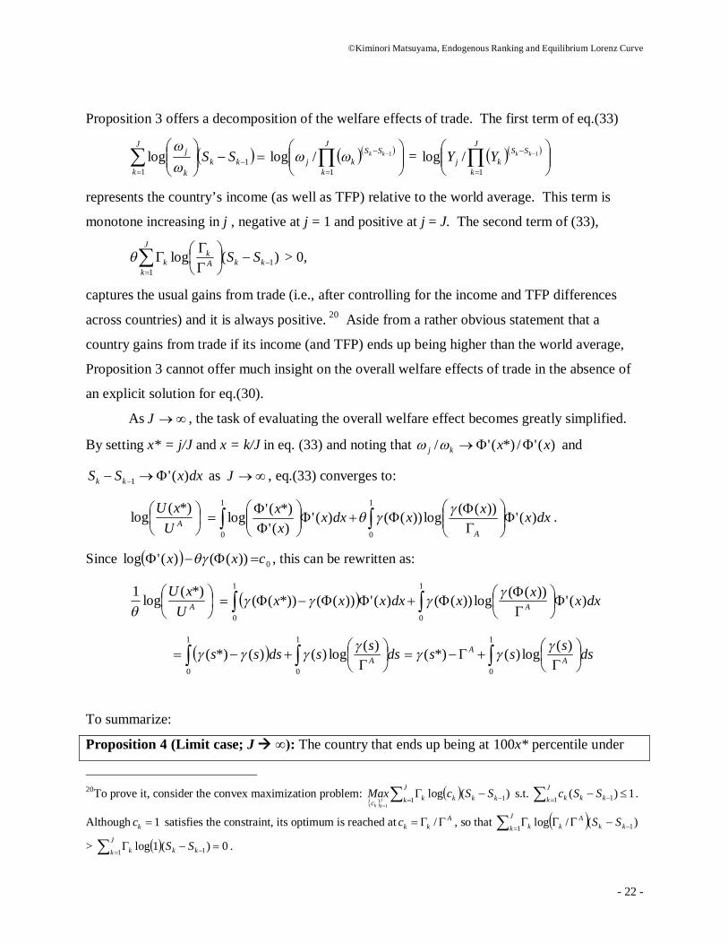
Proposition 3 offers a decomposition of the welfare effects of trade. The first term of eq.(33)
J
kkk
k
j SS1
1log
J
k
SSkj
kk
1
1/log =
J
k
SSkj
kkYY1
1/log
represents the country’s income (as well as TFP) relative to the world average. This term is
monotone increasing in j , negative at j = 1 and positive at j = J. The second term of (33),
J
kkkA
kk SS
11)(log > 0,
captures the usual gains from trade (i.e., after controlling for the income and TFP differences
across countries) and it is always positive. 20 Aside from a rather obvious statement that a
country gains from trade if its income (and TFP) ends up being higher than the world average,
Proposition 3 cannot offer much insight on the overall welfare effects of trade in the absence of
an explicit solution for eq.(30).
As J , the task of evaluating the overall welfare effect becomes greatly simplified.
By setting x* = j/J and x = k/J in eq. (33) and noting that )('/*)('/ xxkj and
dxxSS kk )('1 as J , eq.(33) converges to:
AUxU *)(log
1
0
1
0
)('))((log))(()(')('
*)('log dxxxxdxxxx
A
.
Since 0))(()('log cxx , this can be rewritten as:
AUxU *)(log1
1
0
1
0
)('))((log))(()('))((*))(( dxxxxdxxxx A
1
0
1
0
)(log)()(*)( dsssdsss A
1
0
)(log)(*)( dssss AA
To summarize:
Proposition 4 (Limit case; J ∞): The country that ends up being at 100x* percentile under
20To prove it, consider the convex maximization problem:
J
k kkkkc
SScMaxJkk
1 1)(log1
s.t. 1)(1 1
J
k kkk SSc .
Although 1kc satisfies the constraint, its optimum is reached at Akkc / , so that
J
k kkA
kk SS1 1)(/log
> 0)(1log1 1
J
k kkk SS .
©Kiminori Matsuyama, Endogenous Ranking and Equilibrium Lorenz Curve
- 23 -
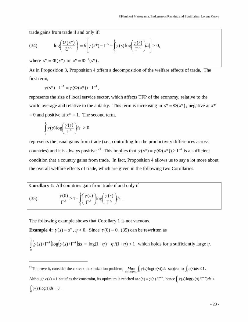
trade gains from trade if and only if:
(34)
AUxU *)(log
1
0
)(log)(*)( dssss AA > 0,
where *)(* xs or *)(* 1 sx .
As in Proposition 3, Proposition 4 offers a decomposition of the welfare effects of trade. The
first term, AA xs *))((*)( ,
represents the size of local service sector, which affects TFP of the economy, relative to the
world average and relative to the autarky. This term is increasing in *)(* xs , negative at x*
= 0 and positive at x* = 1. The second term,
1
0
)(log)( dsss A > 0,
represents the usual gains from trade (i.e., controlling for the productivity differences across
countries) and it is always positive.21 This implies that Axs *))((*)( is a sufficient
condition that a country gains from trade. In fact, Proposition 4 allows us to say a lot more about
the overall welfare effects of trade, which are given in the following two Corollaries.
Corollary 1: All countries gain from trade if and only if
(35)
1
0
)(log)(1)0( dsssAAA
.
The following example shows that Corollary 1 is not vacuous.
Example 4: ss )( , η > 0. Since 0)0( , (35) can be rewritten as
1
0
/)(log/)( dsss AA = 1)1/()1log( , which holds for a sufficiently large η.
21To prove it, consider the convex maximization problem;
1
0]1,0[);())(log()( dsscsMax
ssc subject to 1)(
1
0 dssc .
Although 1)( sc satisfies the constraint, its optimum is reached at Assc /)()( , hence 1
0)/)(log()( dsss A
0)1log()(1
0 dss .
©Kiminori Matsuyama, Endogenous Ranking and Equilibrium Lorenz Curve
- 24 -
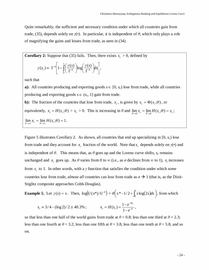
Quite remarkably, the sufficient and necessary condition under which all countries gain from
trade, (35), depends solely on γ(•). In particular, it is independent of θ, which only plays a role
of magnifying the gains and losses from trade, as seen in (34).
Corollary 2: Suppose that (35) fails. Then, there exists cs > 0, defined by
)( cs
1
0
)(log)(1 dsssAA
A ,
such that
a): All countries producing and exporting goods s [0, sc) lose from trade, while all countries
producing and exporting goods s (sc, 1] gain from trade.
b): The fraction of the countries that lose from trade, cx , is given by );( cc xs , or
equivalently, );( cc sHx > cs > 0. This is increasing in θ and ccc ssHx
);(limlim00
;
1);(limlim
cc sHx .
Figure 5 illustrates Corollary 2. As shown, all countries that end up specializing in [0, sc) lose
from trade and they account for cx fraction of the world. Note that cs depends solely on γ(•) and
is independent of θ. This means that, as θ goes up and the Lorenz curve shifts, sc remains
unchanged and cx goes up. As θ varies from 0 to ∞ (i.e., as σ declines from ∞ to 1), cx increases
from cs to 1. In other words, with a γ function that satisfies the condition under which some
countries lose from trade, almost all countries can lose from trade as σ 1 (that is, as the Dixit-
Stiglitz composite approaches Cobb-Douglas).
Example 5; Let ss )( . Then, AUxU /*)(log =
1
02log2/1* dssss , from which
%3.402/)2(log4/3 cs ;
eesHx
cs
cc 11)( ,
so that less than one half of the world gains from trade at θ = 0.8; less than one third at θ = 2.3;
less than one fourth at θ = 3.2; less than one fifth at θ = 3.8, less than one tenth at θ = 5.8, and so
on.

©Kiminori Matsuyama, Endogenous Ranking and Equilibrium Lorenz Curve
- 25 -
3. Two Extensions
The above model can be generalized in many directions. This section offers two
extensions. The first allows a fraction of the consumption goods within each sector to be
nontradeable. By reducing the fraction, this extension enables us to examine how inequality
across countries is affected by globalization through trade in goods. The second allows variable
supply in one of the components in the composite of primary factors, either through factor
accumulation or factor mobility. By changing the share of the variable primary factor in the
composite, this extension enables us to examine how inequality across countries is affected by
technological change that increases importance of human capital or by globalization through
trade in factors.
3.1 Nontradeable Consumption Goods: Globalization through Trade in Goods
In the model of section 2, all consumption goods are assumed to be tradeable. Assume now that
each sector-s produces many varieties, a fraction τ of which is tradeable and a fraction 1−τ is
nontradeable, and that they are aggregated by Cobb-Douglas preferences.22 The expenditure
function is now obtained by replacing ))(log( sP with ))(log()1())(log( sPsP NT for each s
[0,1], where ))}({)( sCMinsP jT is the price of each tradeable good in sector-s, common
across all countries, )()( sCsP jN is the price of each nontradeable good in sector-s, which is
equal to the unit of cost of production in each country.
Instead of going through the entire derivation of the equilibrium, only the key steps will
be highlighted below. Again, let Jjjn
1be a monotone increasing sequence. As before, the
patterns of trade and the free entry condition lead to
(24) 1)(
11
jS
j
j
j
j
nn
. (j = 1, 2, ..., J−1)
22 This specification assumes that the share of local differentiated producer services in sector-s is γ(s) for both nontradeables and tradeables. This assumption is made because, when examining the effect of globalization by changing τ, we do not want the distribution of γ across all tradeable consumption goods to change. However, for some other purposes, it would be useful to consider the case where the distribution of γ among nontradeable consumption goods differ systematically from those among tradeable consumption goods. For example, Matsuyama (1996) allows for such possibility to generate a positive correlation between per capita income and the nontradeable consumption goods prices across countries, similar to the Balassa-Samuelson effect.
©Kiminori Matsuyama, Endogenous Ranking and Equilibrium Lorenz Curve
- 26 -
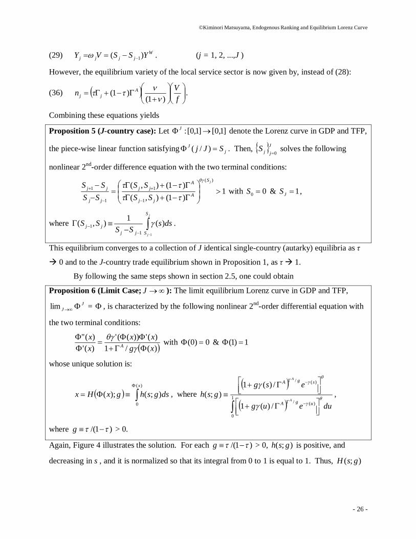
(29) Wjjjj YSSVY )( 1 . (j = 1, 2, ...,J )
However, the equilibrium variety of the local service sector is now given by, instead of (28):
(36)
f
Vn Ajj )1(
)1(
.
Combining these equations yields
Proposition 5 (J-country case): Let ]1,0[]1,0[: J denote the Lorenz curve in GDP and TFP,
the piece-wise linear function satisfying jJ SJj )/( . Then, J
jjS0 solves the following
nonlinear 2nd-order difference equation with the two terminal conditions:
1)1(),()1(),(
)(
1
1
1
1
jS
Ajj
Ajj
jj
jj
SSSS
SSSS
with 00 S & 1JS ,
where
j
j
S
Sjjjj dss
SSSS
1
)(1),(1
1 .
This equilibrium converges to a collection of J identical single-country (autarky) equilibria as τ
0 and to the J-country trade equilibrium shown in Proposition 1, as τ 1.
By following the same steps shown in section 2.5, one could obtain
Proposition 6 (Limit Case; J ): The limit equilibrium Lorenz curve in GDP and TFP, J
J lim = , is characterized by the following nonlinear 2nd-order differential equation with
the two terminal conditions:
)(/1)('))(('
)(')("
xgxx
xx
A
with 0)0( & 1)1(
whose unique solution is:
)(
0
);();(x
dsgshgxHx , where
1
0
)(/
)(/
/)(1
/)(1);(
dueug
esggsh
ugA
sgA
A
A
,
where )1/( g > 0.
Again, Figure 4 illustrates the solution. For each )1/( g > 0, );( gsh is positive, and
decreasing in s , and it is normalized so that its integral from 0 to 1 is equal to 1. Thus, );( gsH
©Kiminori Matsuyama, Endogenous Ranking and Equilibrium Lorenz Curve
- 27 -
is increasing and concave in s , with 0);0( gH and 1);1( gH . Hence, gxHgx ;);( 1 is
increasing and convex in x, with 0);0( g and 1);1( g . It is also easy to check
1);(lim);(lim00
gshgshg
.
Thus, as τ 0, each country converges to the same single-country (autarky) equilibrium and
hence the Lorenz curve converges to the diagonal line, and inequality disappears. Likewise,
1
0
)(
)(
1)();(lim);(lim
due
eshgshgshu
s
g
.
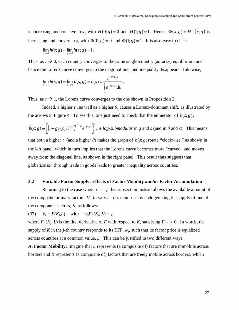
Thus, as τ 1, the Lorenz curve converges to the one shown in Proposition 2.
Indeed, a higher τ , as well as a higher θ, causes a Lorenz-dominant shift, as illustrated by
the arrows in Figure 4. To see this, one just need to check that the numerator of );( gsh ,
)(/
/)(1);(ˆ sgA esggshA
, is log-submodular in g and s (and in θ and s). This means
that both a higher τ (and a higher θ) makes the graph of );( gsh rotate “clockwise,” as shown in
the left panel, which in turn implies that the Lorenz curve becomes more “curved” and moves
away from the diagonal line, as shown in the right panel. This result thus suggests that
globalization through trade in goods leads to greater inequality across countries.
3.2 Variable Factor Supply: Effects of Factor Mobility and/or Factor Accumulation
Returning to the case where τ = 1, this subsection instead allows the available amount of
the composite primary factors, V, to vary across countries by endogenizing the supply of one of
the component factors, K, as follows:
(37) Vj = F(Kj,L) with ωjFK(Kj, L) = ρ.
where FK(Kj, L) is the first derivative of F with respect to K, satisfying FKK < 0. In words, the
supply of K in the j-th country responds to its TFP, ωj, such that its factor price is equalized
across countries at a common value, ρ. This can be justified in two different ways.
A. Factor Mobility: Imagine that L represents (a composite of) factors that are immobile across
borders and K represents (a composite of) factors that are freely mobile across borders, which

©Kiminori Matsuyama, Endogenous Ranking and Equilibrium Lorenz Curve
- 28 -
seek higher return until its return is equalized in equilibrium.23 According to this interpretation,
ρ is an equilibrium rate of return determined endogenously, although it is not necessary to solve
for it when deriving the Lorenz curve.24
B. Factor Accumulation: Reinterpret the structure of the economy as follows. Time is
continuous. All the tradeable goods, s [0,1], are intermediate inputs that goes into the
production of a single final good, Yt, with the Cobb-Douglas function,
1
0))(log(exp dssXY tt
so that its unit cost is
1
0))(log(exp dssPt . The representative agent in each country consumes
and invests the final good to accumulate Kt, so as to maximize
0)( dteCu t
t s.t.
ttt KCY ,
where ρ is the subjective discount rate common across countries. Then, the steady state rate of
return on K is equalized at ρ. 25 According to this interpretation, K may include not only physical
capital but also human capital, and the Lorenz curve derived below represents steady state
inequality across countries.
Again, only the key steps will be shown. Let Jjjn
1be monotone increasing. As before,
Jjj 1
adjust to ensure that there exists a monotone increasing sequence, JjjS
1, defined by S0 =
0, SJ = 1, and
1)(
)(
1
)(
11
j
j
S
j
j
jj
jjj
nn
SCSC
,
such that the j-th country exports s (Sj, Sj+1). This implies that, from (24) and (37),
23Which factors should be considered as mobile or immobile depends on the context. If “countries” are interpreted as smaller geographical units such as “metropolitan areas,” K may include not only capital but also labor, with L representing the immobile “land.” Although labor is commonly treated as an immobile factor in the trade literature, we will later consider the possibility of trade in factors, in which case certain types of labor should be included among mobile factors. 24Also, Yj = Vj = ωjF(Kj, L) should be now interpreted as GDP of the economy, not GNP, and Kj is the amount of K used in the j-th country, not the amount of K owned by the representative agent in the j-th country. This also means that the LHS of the budget constraint in the j-th country should be its GNP, not its GDP (Yj). However, calculating the distributions of GDP (Yj), TFP (ωj), and Kj/L does not require to use the budget constraint for each country, given that all consumption goods are tradeable (τ = 1). The analysis would be more involved if τ < 1. 25The intertemporal resource constraint assumes not only that K is immobile but also that international lending and borrowing is not possible. Of course, these restrictions are not binding in steady state, because the rate of return is equalized across countries at ρ
©Kiminori Matsuyama, Endogenous Ranking and Equilibrium Lorenz Curve
- 29 -
1),(
),()(
11
1
jS
j
j
j
j
jK
jK
nn
LKFLKF
which implies that Jjj 1
, JjjK
1, and J
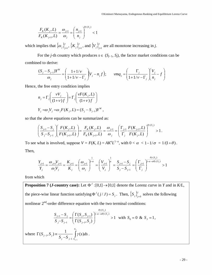
jjV1 are all monotone increasing in j.
For the j-th country which produces s (Sj−1, Sj), the factor market conditions can be
combined to derive:
fnVYSS
jjjj
Wjj
/11/11)( 1 ;
f
nV
mqj
j
j
jj
/11
Hence, the free entry condition implies
fLKF
fV
n jj
jjj )1(
),()1(
Wjjjjjjj YSSLKFVY )(),( 1 ,
so that the above equations can be summarized as:
),(),(
11
1
LKFLKF
SSSS
j
j
jj
jj 1),(),(
),(),(
)(
111
1
jS
j
j
j
j
j
j
jK
jK
LKFLKF
LKFLKF
.
To see what is involved, suppose V = F(K, L) = AKαL1−α, with 0 < < /11 = )1/(1 .
Then,
1
1
1
11
1
11111
jj
jj
j
j
j
j
j
j
jj
jj
j
j
SSSS
VV
KK
VV
YY
1)(1
)(
1
j
j
SS
j
j
from which
Proposition 7 (J-country case): Let ]1,0[]1,0[: J denote the Lorenz curve in Y and in K/L,
the piece-wise linear function satisfying jJ SJj )/( . Then, J
jjS0 solves the following
nonlinear 2nd-order difference equation with the two terminal conditions:
1),(),( )(1
)(
1
1
1
1
j
j
SS
jj
jj
jj
jj
SSSS
SSSS
with 00 S & 1JS ,
where
j
j
S
Sjjjj dss
SSSS
1
)(1),(1
1 .
©Kiminori Matsuyama, Endogenous Ranking and Equilibrium Lorenz Curve
- 30 -
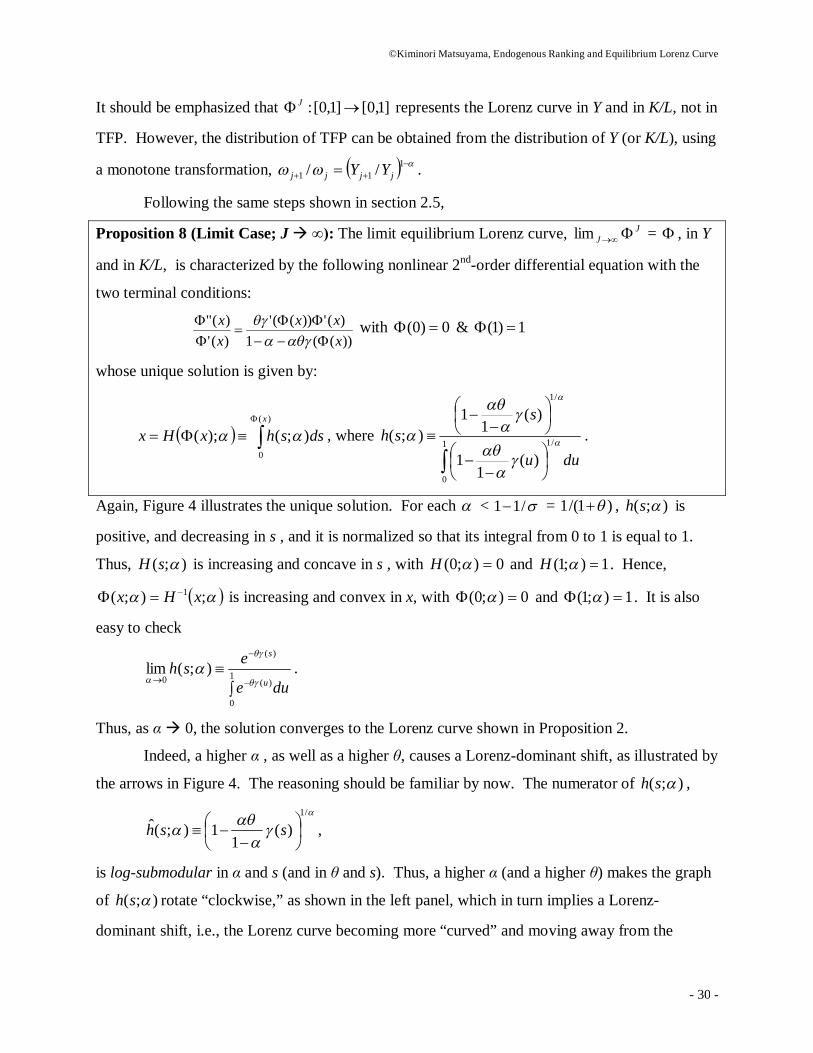
It should be emphasized that ]1,0[]1,0[: J represents the Lorenz curve in Y and in K/L, not in
TFP. However, the distribution of TFP can be obtained from the distribution of Y (or K/L), using
a monotone transformation, 111 // jjjj YY .
Following the same steps shown in section 2.5,
Proposition 8 (Limit Case; J ∞): The limit equilibrium Lorenz curve, JJ lim = , in Y
and in K/L, is characterized by the following nonlinear 2nd-order differential equation with the
two terminal conditions:
))((1)('))(('
)(')("
xxx
xx
with 0)0( & 1)1(
whose unique solution is given by:
)(
0
);();(x
dsshxHx , where
1
0
/1
/1
)(1
1
)(1
1);(
duu
ssh
.
Again, Figure 4 illustrates the unique solution. For each < /11 = )1/(1 , );( sh is
positive, and decreasing in s , and it is normalized so that its integral from 0 to 1 is equal to 1.
Thus, );( sH is increasing and concave in s , with 0);0( H and 1);1( H . Hence,
;);( 1 xHx is increasing and convex in x, with 0);0( and 1);1( . It is also
easy to check
1
0
)(
)(
0);(lim
due
eshu
s
.
Thus, as α 0, the solution converges to the Lorenz curve shown in Proposition 2.
Indeed, a higher α , as well as a higher θ, causes a Lorenz-dominant shift, as illustrated by
the arrows in Figure 4. The reasoning should be familiar by now. The numerator of );( sh ,
/1
)(1
1);(ˆ
ssh ,
is log-submodular in α and s (and in θ and s). Thus, a higher α (and a higher θ) makes the graph
of );( sh rotate “clockwise,” as shown in the left panel, which in turn implies a Lorenz-
dominant shift, i.e., the Lorenz curve becoming more “curved” and moving away from the

©Kiminori Matsuyama, Endogenous Ranking and Equilibrium Lorenz Curve
- 31 -
diagonal line, as shown in the right panel. This result suggests that skill-biased technological
change that increases the share of human capital and reduces the share of raw labor in
production, or globalization through trade in some factors, both of which can be interpreted as an
increase in α, could lead to greater inequality across countries.
4. Concluding Remarks
In cross-section of countries, the rich tend to have higher TFPs and higher capital-labor
ratios. Such empirical findings are typically interpreted as the causality from TFPs and/or
capital-labor ratios to income under two maintained hypotheses; i) these countries offer
independent observations and ii) any variations in endogenous variables across countries would
disappear in the absence of any exogenous sources of variations across countries. The model
presented above offers some cautions for such an interpretation of cross-country variations.
Despite that countries are ex-ante identical, the model predicts that a strict ranking of countries in
income, TFPs, and capital-labor ratios (and other endogenous variables) emerge endogenously,
and these variables are all jointly determined, and (perfectly) correlated across countries. This
occurs because the countries end up sorting themselves into specializing in different sets of
tradeable sectors. In other words, some countries become richer (poorer) than others partly
because they trade with poorer (richer) countries, so these countries do not offer independent
observations. Of course, there have been other studies that deliver a similar message. In contrast
to such earlier studies, which all used a highly stylized framework, the model here has advantage
that it allows for any finite number of countries and offers a full characterization of the
equilibrium Lorenz curve across countries in an analytically tractable manner.
As a model of endogenous inequality of nations, the framework presented in this paper is
used to examine how globalization or technological change might change the endogenous
components of heterogeneities across countries. Needless to say, there are exogenous sources of
heterogeneities across countries, e.g., climate, natural endowments, location, etc. The logic of
symmetry-breaking does not suggest that such exogenous heterogeneities are unimportant. Quite
on the contrary, symmetry-breaking is a magnification mechanism. It suggests that even small
amounts of exogenous differences can be amplified to create large observed differences across
countries in income, TFPs, capital-labor ratios, and other endogenous variables.

©Kiminori Matsuyama, Endogenous Ranking and Equilibrium Lorenz Curve
- 32 -
S s 1
Home Exports Foreign Exports
O
1
C(s)/C*(s)
Figure 1: Comparative Advantage and Patterns of Trade in the Two-Country World
S j−1 s
1
Cj−1(s)/Cj(s) Cj(s)/Cj+1(s)
Sj
sj
1 O
Figure 2: Comparative Advantage and Patterns of Trade in the J-country World

©Kiminori Matsuyama, Endogenous Ranking and Equilibrium Lorenz Curve
- 33 -
O 1
s
h(s)
O 1
s=Ф(x) =H−1(s)
1
x=H(s) = Φ−1(s)
Figure 4: Limit Equilibrium Lorenz Curve, Φ(x), and its Lorenz-dominant Shift
2/4 O
1
1 3/4 1/4
S3
S2
S1
s4
s3
s2
Figure 3: Equilibrium Lorenz curve, ΦJ: A Graphic Illustration for J = 4

©Kiminori Matsuyama, Endogenous Ranking and Equilibrium Lorenz Curve
- 34 -
sc O 1
Ф(x)=s
1
x=H(s)
xc
xc
Figure 5: A Graphic Illustration of Corollary 2

©Kiminori Matsuyama, Endogenous Ranking and Equilibrium Lorenz Curve
- 35 -
References: Acemoglu, D., Introduction to Modern Economic Growth, Princeton University Press, 2008. Acemoglu, D., and J. Ventura, “The World Income Distribution,” Quarterly Journal of Economics,
117 (2002), 659-694. Ciccone, A., and K. Matsuyama, “Start-up Costs and Pecuniary Externalities as Barriers to
Economic Development,” Journal of Development Economics, 1996, 49, 33-59. Combes, P.-P., T. Mayer and J. Thisse, Economic Geography, Princeton University Press, 2008. Costinot, A., “An Elementary Theory of Comparative Advantage,” Econometrica, 2009, 1165-
1192. Costinot, A., and J. Vogel, “Matching and Inequality in the World Economy,” Journal of
Political Economy, 118, August 2010, 747-786. Dixit, A. K., and J. E. Stiglitz, “Monopolistic Competition and Optimum Product Diversity,”
American Economic Review, 1977, 297-308. Dornbusch, R., S. Fischer and P. A. Samuelson, “Comparative Advantage, Trade, and Payments
in a Ricardian Model with a Continuum of Goods,” American Economic Review, 67 (1977), 823-839.
Ethier, W., “National and International Returns to Scale in the Modern Theory of International Trade,” American Economic Review, 72, 1982, 389-405. a)
Ethier, W., “Decreasing Costs in International Trade and Frank Graham’s Argument for Protection,” Econometrica, 50, 1982, 1243-1268. b)
Fujita, M., P., Krugman, P. and A. Venables, The Spatial Economy, MIT Press, 1999. Grossman, G., and E. Helpman, “Quality Ladders in the Theory of Growth,” Review of
Economic Studies, January 1991, 43-61. Helpman, E., “Increasing Returns, Imperfect Markets and Trade Theory,” Chapter 7 in
Handbook of International Economics, edited by R. Jones and P. Kenen, 1986. Ioannides, Y., “Emergence,” in L. Blume and S. Durlauf, eds., New Palgrave Dictionary of
Economics, 2nd Edition, Palgrave Macmillan, 2008. Jovanovic, B., “Vintage Capital and Inequality,” Review of Economic Dynamics, (1998), 497-
530. Jovanovic, B., “The Technology Cycle and Inequality,” Review of Economic Studies, (2009)
707-729. Krugman, P. and A. Venables, “Globalization and Inequality of Nations,” Quarterly Journal of
Economics, 110 (1995), 857–80. Lewis, W.A. The Evolution of the International Economic Order, Princeton, Princeton University
Press, 1977. Matsuyama, K. (1991): “Increasing Returns, Industrialization and Indeterminacy of
Equilibrium,” Quarterly Journal of Economics, 106, 617-650. Matsuyama, K., “Agricultural Productivity, Comparative Advantage, and Economic Growth,
Journal of Economic Theory, 58, December 1992, 317-334. Matsuyama, K., “Complementarities and Cumulative Processes in Models of Monopolistic
Competition,” Journal of Economic Literature, 1995. Matsuyama, K., “Why Are There Rich and Poor Countries?: Symmetry-Breaking in the World
Economy,” Journal of the Japanese and International Economies, 10 (1996), 419-439. Matsuyama, K., “Explaining Diversity: Symmetry-Breaking in Complementarity Games,”
American Economic Review, 2002, 92, 241-246.
©Kiminori Matsuyama, Endogenous Ranking and Equilibrium Lorenz Curve
- 36 -
Matsuyama, K., “Symmetry-Breaking” in L. Blume and S. Durlauf, eds., New Palgrave
Dictionary of Economics, 2nd Edition, Palgrave Macmillan, 2008. Matsuyama, K., and T. Takahashi, “Self-Defeating Regional Concentration,” Review of
Economic Studies, 65 (April 1998): 211-234. Murhpy, K., A. Shleifer, and R. Vishny, “Industrialization and the Big Push,” Journal of Political
Economy, October 1989, 1003-1026. Myrdal, G. Economic Theory and Underdeveloped Regions, Duckworth, 1957. Rodríguez-Clare, “Division of Labor and Economic Development,” Journal of Development
Economics, 1996, 49, 3-32. Romer, P., “Growth Based on Increasing Returns Due to Specialization,” American Economic
Review, 77 (1987), 56-62. Topkis, D., Supermodularity and Complementarity, Princeton University Press, 1998. Ventura, J., “A Global View of Economic Growth,” in P. Aghion and S. N. Durlauf, eds.,
Handbook of Economic Growth. Vol, IB, Amsterdam, Elsevier BV, 2005. Williamson, Jeffrey G. Trade and Poverty: When the Third World Fell Behind, MIT Press, 2011.


