
EPID 600; Class 10 Effect measure modification
University of Michigan School of Public Health
1
Effect measure modification
Situation where measure of effect changes over the value of some other variable Stated another way, where the effect of interest (as typically expressed by a measure of association) is heterogenous over a third variable
2
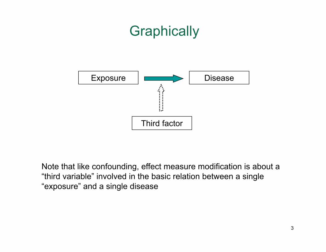
Graphically
Exposure Disease
Third factor
Note that like confounding, effect measure modification is about a “third variable” involved in the basic relation between a single “exposure” and a single disease
3
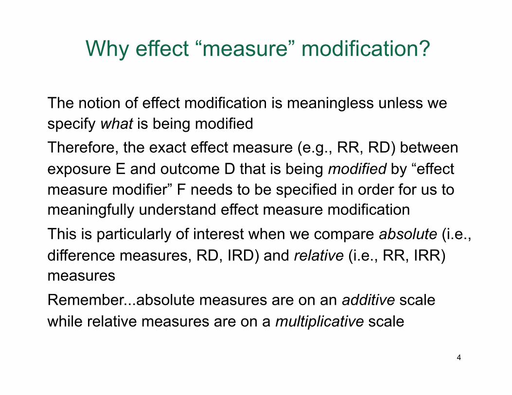
Why effect “measure” modification?
The notion of effect modification is meaningless unless we specify what is being modified Therefore, the exact effect measure (e.g., RR, RD) between exposure E and outcome D that is being modified by “effect measure modifier” F needs to be specified in order for us to meaningfully understand effect measure modification This is particularly of interest when we compare absolute (i.e., difference measures, RD, IRD) and relative (i.e., RR, IRR) measures Remember...absolute measures are on an additive scale while relative measures are on a multiplicative scale
4
Example
No exposure to ceramic dust
Exposure to ceramic dust
Smokers 10 50
Non-smokers 5 5
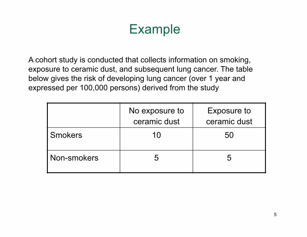
A cohort study is conducted that collects information on smoking, exposure to ceramic dust, and subsequent lung cancer. The table below gives the risk of developing lung cancer (over 1 year and expressed per 100,000 persons) derived from the study
5
Example
No exposure to ceramic dust
Exposure to ceramic dust
Smokers 10 50
Non-smokers 5 5
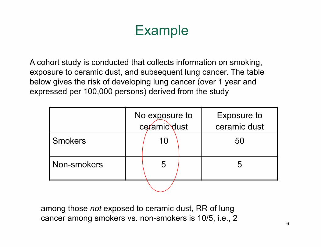
A cohort study is conducted that collects information on smoking, exposure to ceramic dust, and subsequent lung cancer. The table below gives the risk of developing lung cancer (over 1 year and expressed per 100,000 persons) derived from the study
among those not exposed to ceramic dust, RR of lung cancer among smokers vs. non-smokers is 10/5, i.e., 2
6
Example
No exposure to ceramic dust
Exposure to ceramic dust
Smokers 10 50
Non-smokers 5 5
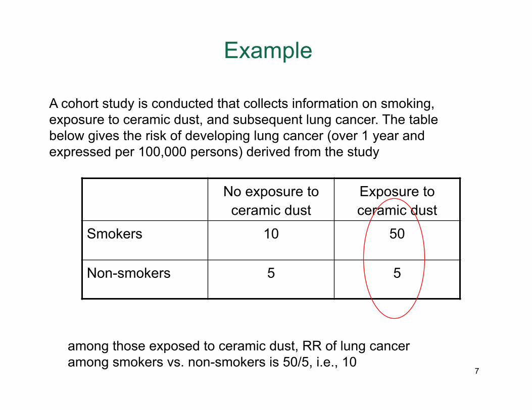
A cohort study is conducted that collects information on smoking, exposure to ceramic dust, and subsequent lung cancer. The table below gives the risk of developing lung cancer (over 1 year and expressed per 100,000 persons) derived from the study
among those exposed to ceramic dust, RR of lung cancer among smokers vs. non-smokers is 50/5, i.e., 10
7
Therefore...
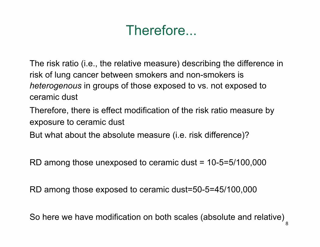
The risk ratio (i.e., the relative measure) describing the difference in risk of lung cancer between smokers and non-smokers is heterogenous in groups of those exposed to vs. not exposed to ceramic dust Therefore, there is effect modification of the risk ratio measure by exposure to ceramic dust But what about the absolute measure (i.e. risk difference)?
RD among those unexposed to ceramic dust = 10-5=5/100,000
RD among those exposed to ceramic dust=50-5=45/100,000
So here we have modification on both scales (absolute and relative) 8
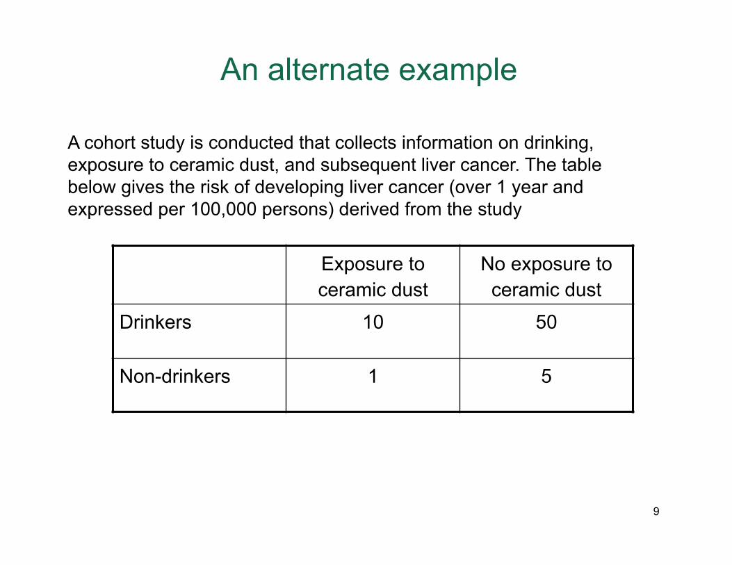
An alternate example
Exposure to ceramic dust
No exposure to ceramic dust
Drinkers 10 50
Non-drinkers 1 5
A cohort study is conducted that collects information on drinking, exposure to ceramic dust, and subsequent liver cancer. The table below gives the risk of developing liver cancer (over 1 year and expressed per 100,000 persons) derived from the study
9
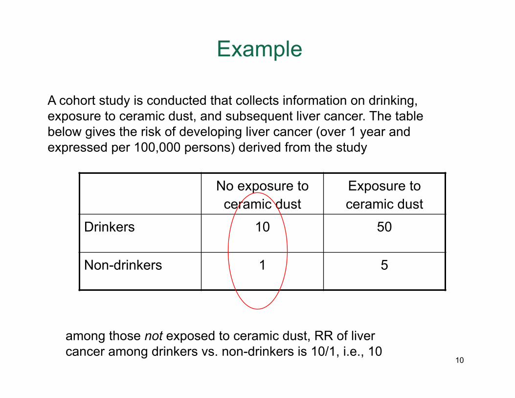
Example
No exposure to ceramic dust
Exposure to ceramic dust
Drinkers 10 50
Non-drinkers 1 5
A cohort study is conducted that collects information on drinking, exposure to ceramic dust, and subsequent liver cancer. The table below gives the risk of developing liver cancer (over 1 year and expressed per 100,000 persons) derived from the study
among those not exposed to ceramic dust, RR of liver cancer among drinkers vs. non-drinkers is 10/1, i.e., 10
10
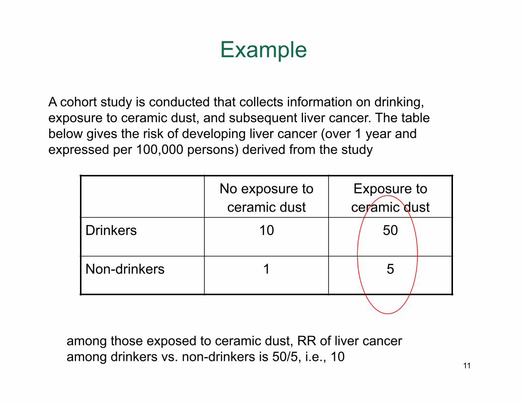
Example
No exposure to ceramic dust
Exposure to ceramic dust
Drinkers 10 50
Non-drinkers 1 5
A cohort study is conducted that collects information on drinking, exposure to ceramic dust, and subsequent liver cancer. The table below gives the risk of developing liver cancer (over 1 year and expressed per 100,000 persons) derived from the study
among those exposed to ceramic dust, RR of liver cancer among drinkers vs. non-drinkers is 50/5, i.e., 10
11
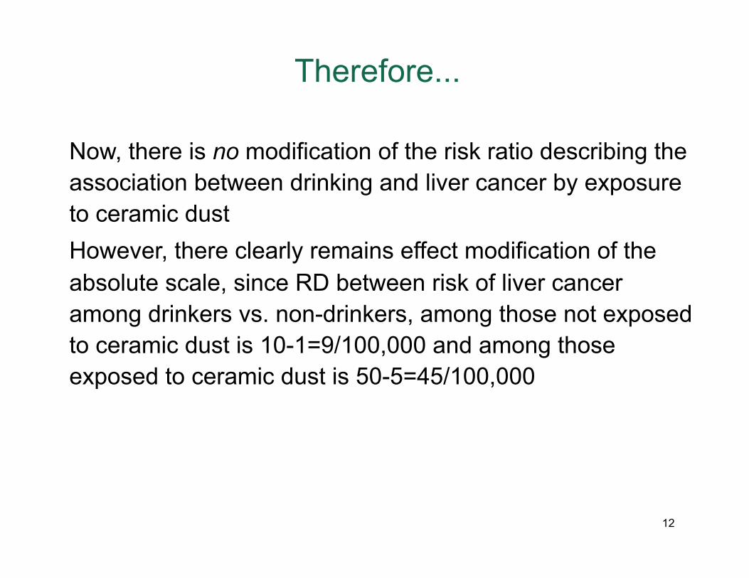
Therefore...
Now, there is no modification of the risk ratio describing the association between drinking and liver cancer by exposure to ceramic dust However, there clearly remains effect modification of the absolute scale, since RD between risk of liver cancer among drinkers vs. non-drinkers, among those not exposed to ceramic dust is 10-1=9/100,000 and among those exposed to ceramic dust is 50-5=45/100,000
12
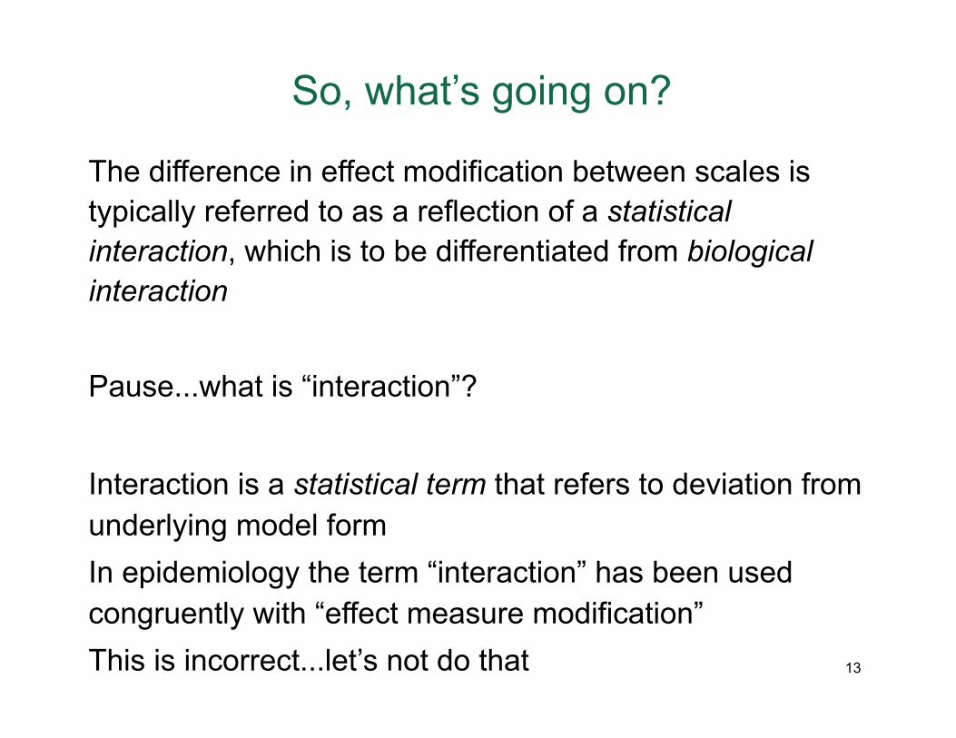
So, what’s going on?
The difference in effect modification between scales is typically referred to as a reflection of a statistical interaction, which is to be differentiated from biological interaction
Pause...what is “interaction”?
Interaction is a statistical term that refers to deviation from underlying model form In epidemiology the term “interaction” has been used congruently with “effect measure modification” This is incorrect...let’s not do that 13
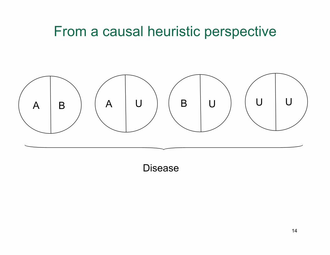
From a causal heuristic perspective
UB UU
Disease
BA UA
14
Conceptually, statistical interaction (1)
Statistical interaction then refers to deviation from the way we are specifying our relation between variables of interest
A. Positive statistical interaction refers to the situation where the association between two variables is greater than might be expected given the way a model is specified Note, put another way, the third variable accentuates the relation between exposure and outcome
B. Negative statistical interaction refers to a situation where the association between two variables is less than might be expected
Note, put another way, the third variable diminishes the relation between exposure and outcome
15
Conceptually, statistical interaction (2)
Given that statistical interaction depends on how we are specifying the “model” that describes the relation between variables of interest, then statistical interaction can come in two forms, both dependent on comparing expected vs. observed joint effects of our variables acting independently or together
A. Additive interaction is when the joint effect of exposure and third variable is not equivalent to the arithmetic sum of the independent effects (component effects) measured by the RD or IRD
B. Multiplicative interaction is when the joint effect of exposure and third variable is not equivalent to the multiplication of the independent effects (component effects) measured by the RR or IRR
16
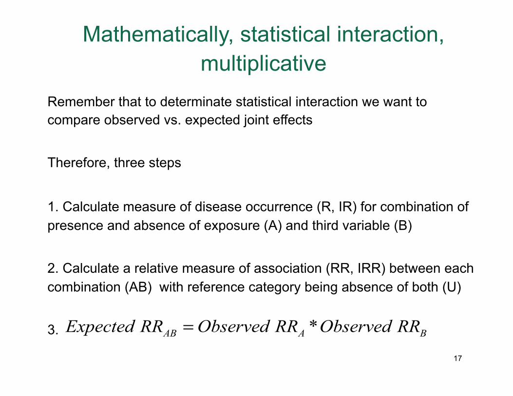
Mathematically, statistical interaction, multiplicative
Remember that to determinate statistical interaction we want to compare observed vs. expected joint effects
Therefore, three steps
1. Calculate measure of disease occurrence (R, IR) for combination of presence and absence of exposure (A) and third variable (B)
2. Calculate a relative measure of association (RR, IRR) between each combination (AB) with reference category being absence of both (U)
3. *AB A BExpected RR Observed RR Observed RR=
17
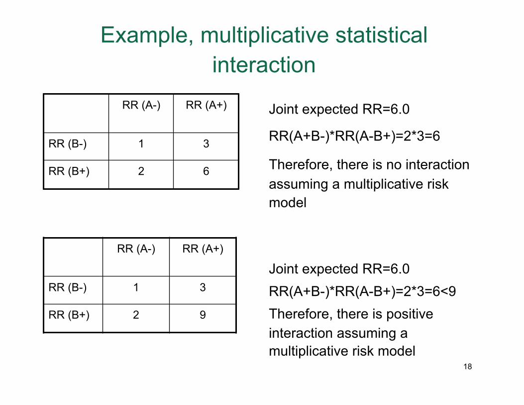
Example, multiplicative statistical interaction
RR (A-) RR (A+)
RR (B-) 1 3
RR (B+) 2 6
RR (A-) RR (A+)
RR (B-) 1 3
RR (B+) 2 9
Joint expected RR=6.0
RR(A+B-)*RR(A-B+)=2*3=6
Therefore, there is no interaction assuming a multiplicative risk model
Joint expected RR=6.0 RR(A+B-)*RR(A-B+)=2*3=6<9 Therefore, there is positive interaction assuming a multiplicative risk model
18
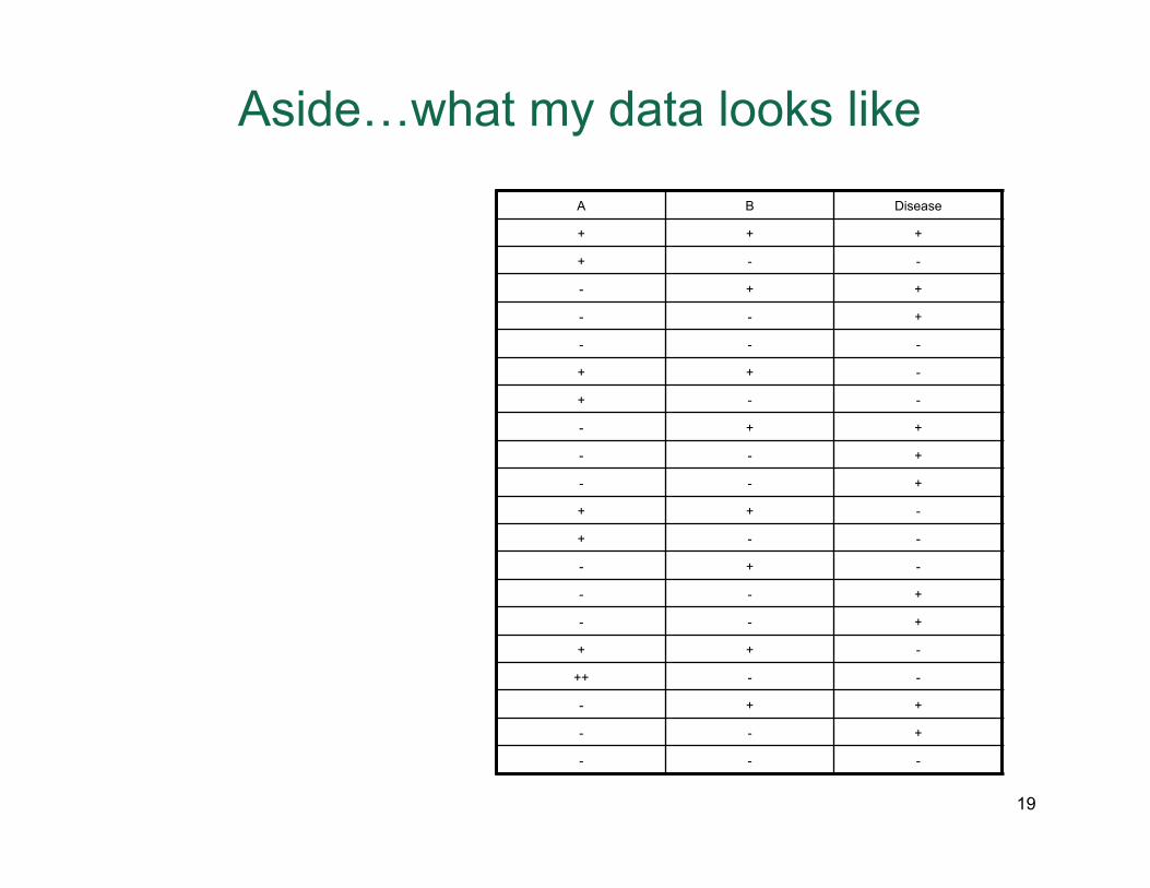
Aside…what my data looks like
A B Disease
+ + +
+ - -
- + +
- - +
- - -
+ + -
+ - -
- + +
- - +
- - +
+ + -
+ - -
- + -
- - +
- - +
+ + -
++ - -
- + +
- - +
- - -
19
Aside…what my data looks like
A B Disease
+ + +
+ - -
- + +
- - +
- - -
+ + -
+ - -
+ + +
- - +
- - +
+ + -
+ - -
- + -
- + +
- - +
+ + -
+ - -
- + +
- - +
- - -
20
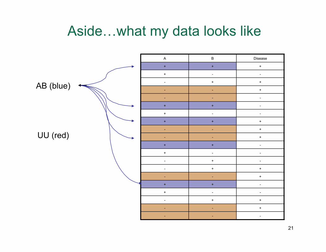
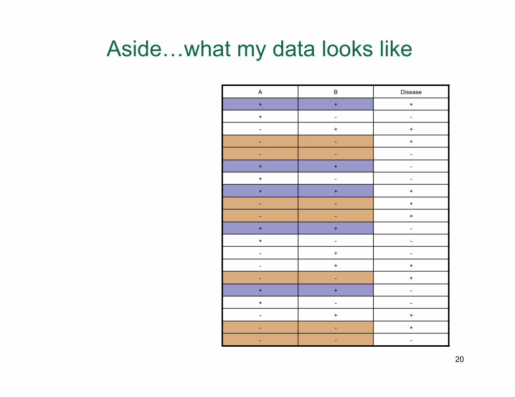
Aside…what my data looks like
A B Disease
+ + +
+ - -
- + +
- - +
- - -
+ + -
+ - -
+ + +
- - +
- - +
+ + -
+ - -
- + -
- + +
- - +
+ + -
+ - -
- + +
- - +
- - -
AB (blue)
UU (red)
21
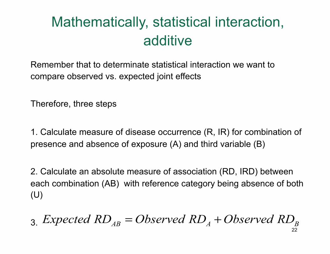
Mathematically, statistical interaction, additive
Remember that to determinate statistical interaction we want to compare observed vs. expected joint effects
Therefore, three steps
1. Calculate measure of disease occurrence (R, IR) for combination of presence and absence of exposure (A) and third variable (B)
2. Calculate an absolute measure of association (RD, IRD) between each combination (AB) with reference category being absence of both (U)
3. AB A BExpected RD Observed RD Observed RD= +22
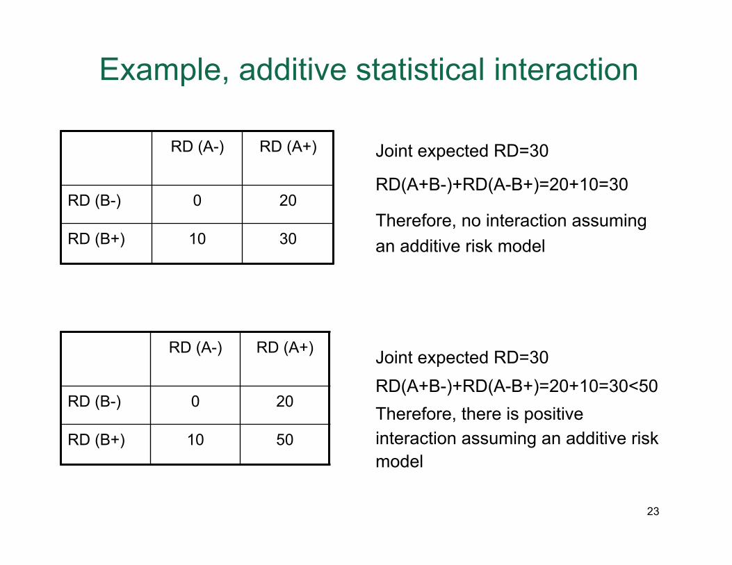
Example, additive statistical interaction
RD (A-) RD (A+)
RD (B-) 0 20
RD (B+) 10 30
RD (A-) RD (A+)
RD (B-) 0 20
RD (B+) 10 50
Joint expected RD=30
RD(A+B-)+RD(A-B+)=20+10=30
Therefore, no interaction assuming an additive risk model
Joint expected RD=30 RD(A+B-)+RD(A-B+)=20+10=30<50 Therefore, there is positive interaction assuming an additive risk model
23
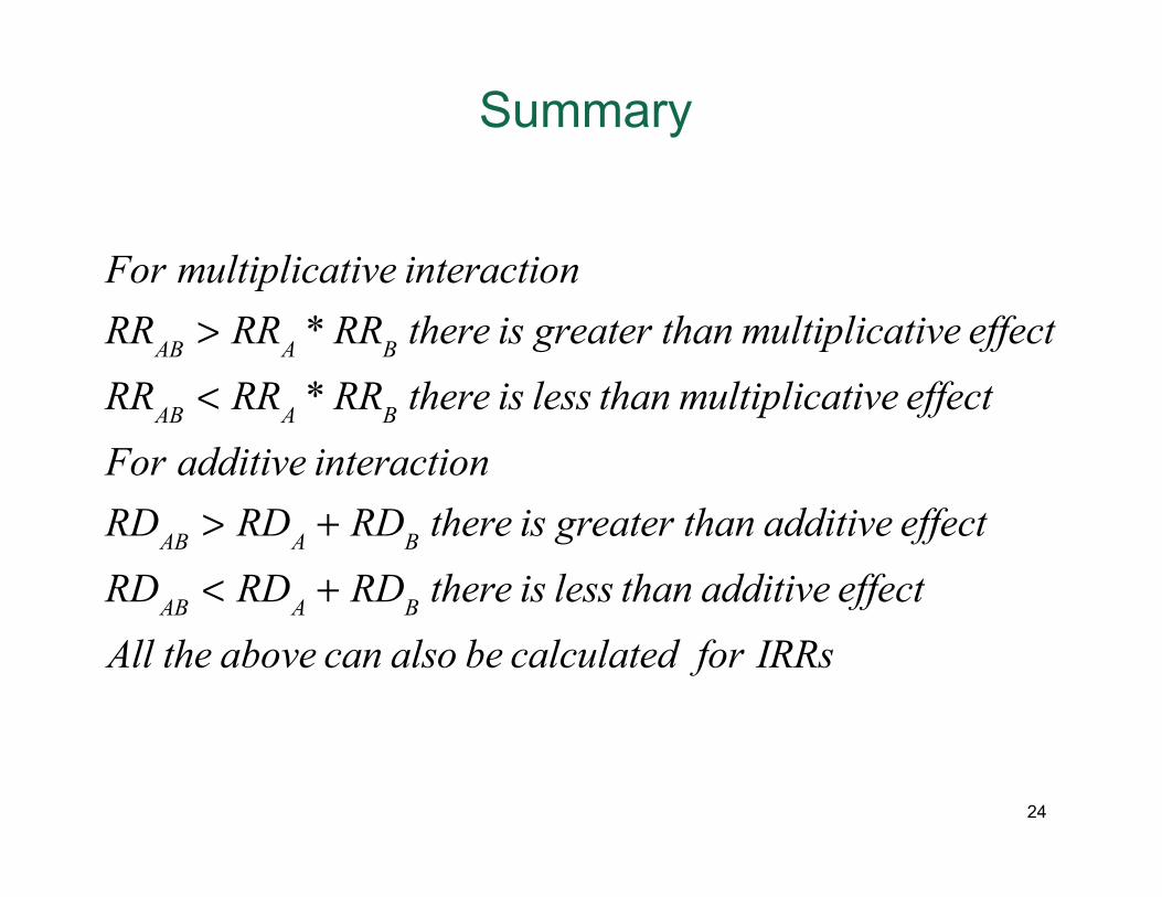
Summary
For multiplicative interactionRRAB > RRA * RRB there is greater than multiplicative effectRRAB < RRA * RRB there is less than multiplicative effectFor additive interactionRDAB > RDA + RDB there is greater than additive effectRDAB < RDA + RDB there is less than additive effectAll the above can also be calculated for IRRs
24
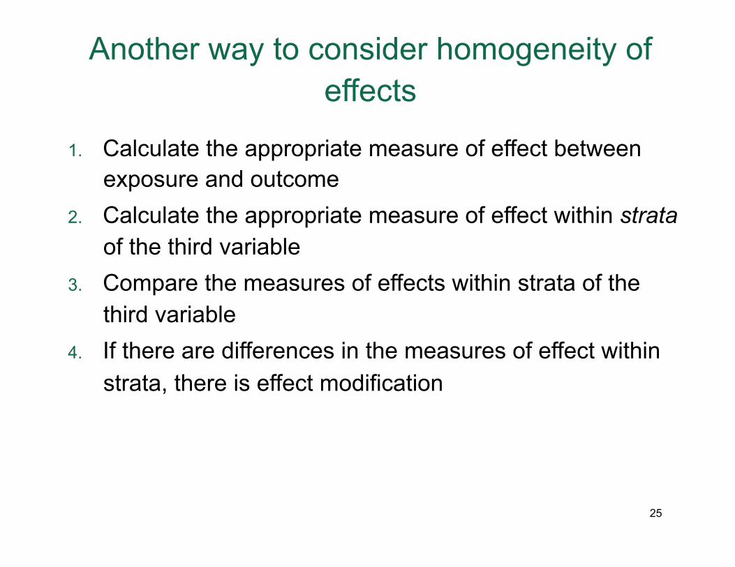
Another way to consider homogeneity of effects
1. Calculate the appropriate measure of effect between exposure and outcome
2. Calculate the appropriate measure of effect within strata of the third variable
3. Compare the measures of effects within strata of the third variable
4. If there are differences in the measures of effect within strata, there is effect modification
25
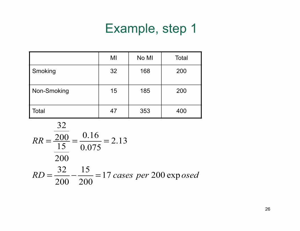
Example, step 1
MI No MI Total
Smoking 32 168 200
Non-Smoking 15 185 200
Total 47 353 400
320.16200 2.1315 0.075
20032 15 17 200 exp200 200
RR
RD cases per osed
= = =
= − =
26
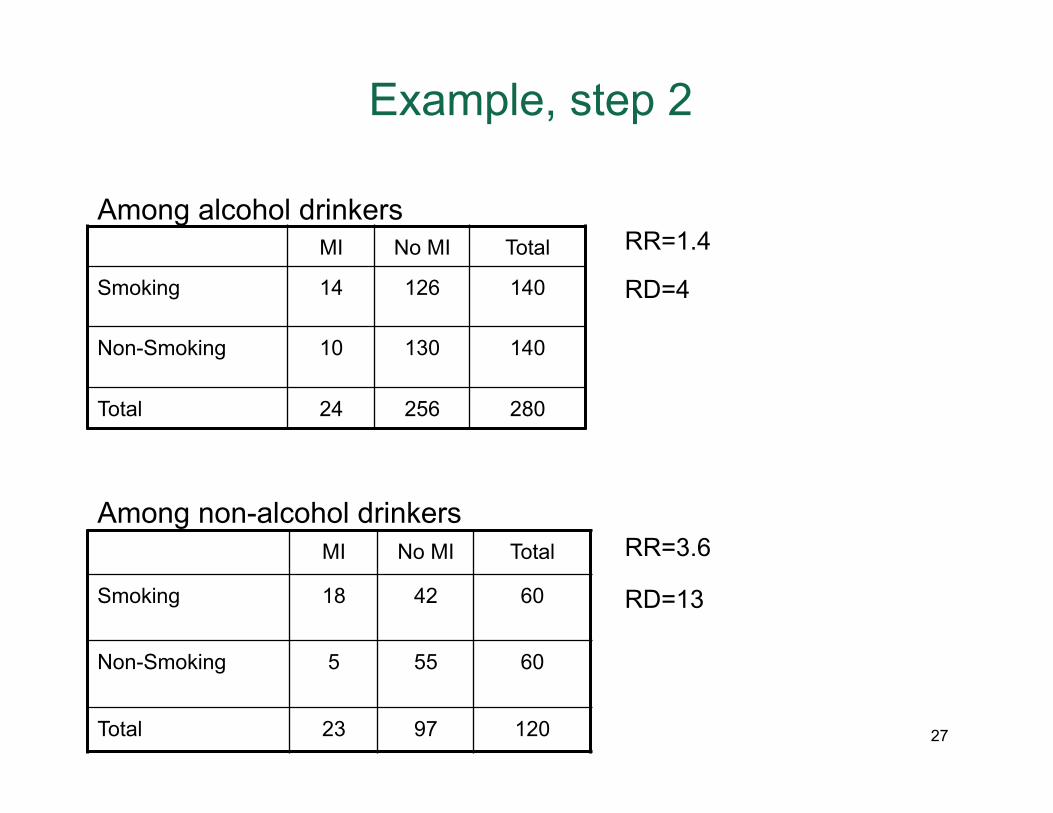
Example, step 2
MI No MI Total
Smoking 14 126 140
Non-Smoking 10 130 140
Total 24 256 280
Among alcohol drinkers
MI No MI Total
Smoking 18 42 60
Non-Smoking 5 55 60
Total 23 97 120
Among non-alcohol drinkers
RR=1.4
RD=4
RR=3.6
RD=13
27
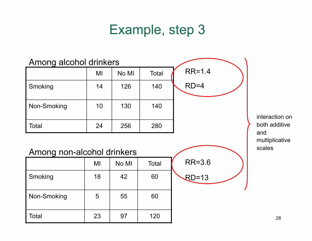
Example, step 3
MI No MI Total
Smoking 14 126 140
Non-Smoking 10 130 140
Total 24 256 280
Among alcohol drinkers
MI No MI Total
Smoking 18 42 60
Non-Smoking 5 55 60
Total 23 97 120
Among non-alcohol drinkers
RR=1.4
RD=4
RR=3.6
RD=13
interaction on both additive and multiplicative scales
28
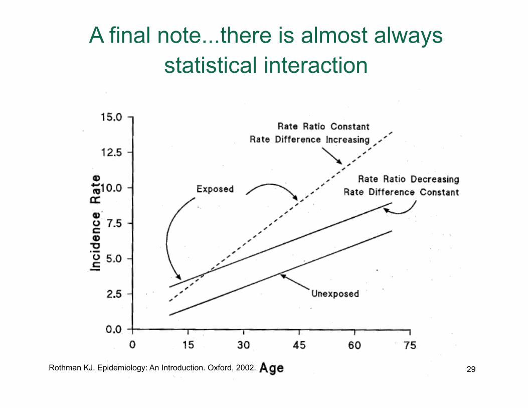
A final note...there is almost always statistical interaction
Rothman KJ. Epidemiology: An Introduction. Oxford, 2002. 29
Stroke: geography or race?
8 southern US states are consistently found to have higher stroke mortality, and termed the “stroke belt” Stroke mortality rates are about 50% higher in blacks as compared to whites Is it black race or southern geography that explain stroke patterns in the US? Or do these two trends both interact in some way?
Howard et al. Regional differences in African American’s high risk for stroke: the remarkable burden of stroke for southern African Americans. Ann Epidemiol. 2007; 17: 689-696.
30
Stroke: geography or race?
Set up: Stroke mortality rates were calculated for sex and age strata on the basis of US vital statistics 1997-2001 Investigators looked at the patterns in southern vs non-southern states They compared the ratio of white and black mortality rates They compared the “excess” mortality in the south vs. non-south for each race They compared the difference in the excess between the two races
Howard et al. Regional differences in African American’s high risk for stroke: the remarkable burden of stroke for southern African Americans. Ann Epidemiol. 2007; 17: 689-696.
31
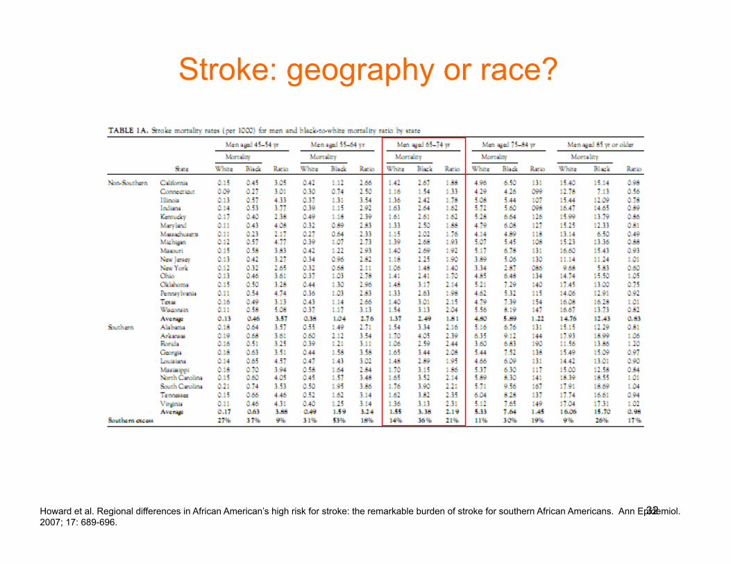
Stroke: geography or race?
Howard et al. Regional differences in African American’s high risk for stroke: the remarkable burden of stroke for southern African Americans. Ann Epidemiol. 2007; 17: 689-696.
32
Stroke: geography or race?
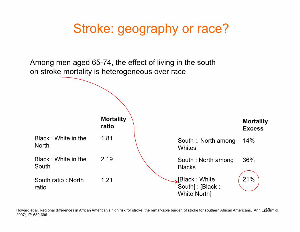
Mortality Excess
South :. North among Whites
14%
South : North among Blacks
36%
[Black : White South] : [Black : White North]
21%
Among men aged 65-74, the effect of living in the south on stroke mortality is heterogeneous over race
Mortality ratio
Black : White in the North
1.81
Black : White in the South
2.19
South ratio : North ratio
1.21
Howard et al. Regional differences in African American’s high risk for stroke: the remarkable burden of stroke for southern African Americans. Ann Epidemiol. 2007; 17: 689-696.
33
What about biologic interaction?
We have now summarized the notion of statistical interaction which shows clearly that statistical interaction depends primarily on choice of specification of effect measure However, earlier we introduced the notion of biologic interaction Biologic interaction between component causes A and B means that the effect of A on an individual depends on the presence/absence (or level of) B There might then be merit to understand the implications of biologic interaction, and how they are (or are not) different than those of statistical interaction
34
Understanding biologic interaction
Assume we are interested in two variables A and B Assume that a particular disease can be caused by variables A and B and a set of other unspecified variables U Therefore, there are 4 ways in which the disease can be produced, that is ABU, AU, BU, and U This has clear analogs in sufficient cause model If we buy above argument that disease production is a function of four causes (ABU, AU, BU, and U) then surely disease production is all explained by the addition of these 4 causes Hence, departure from additivity on the risk scale for two exposures is an indication of biologic interaction in the population
35
Defining biologic interaction
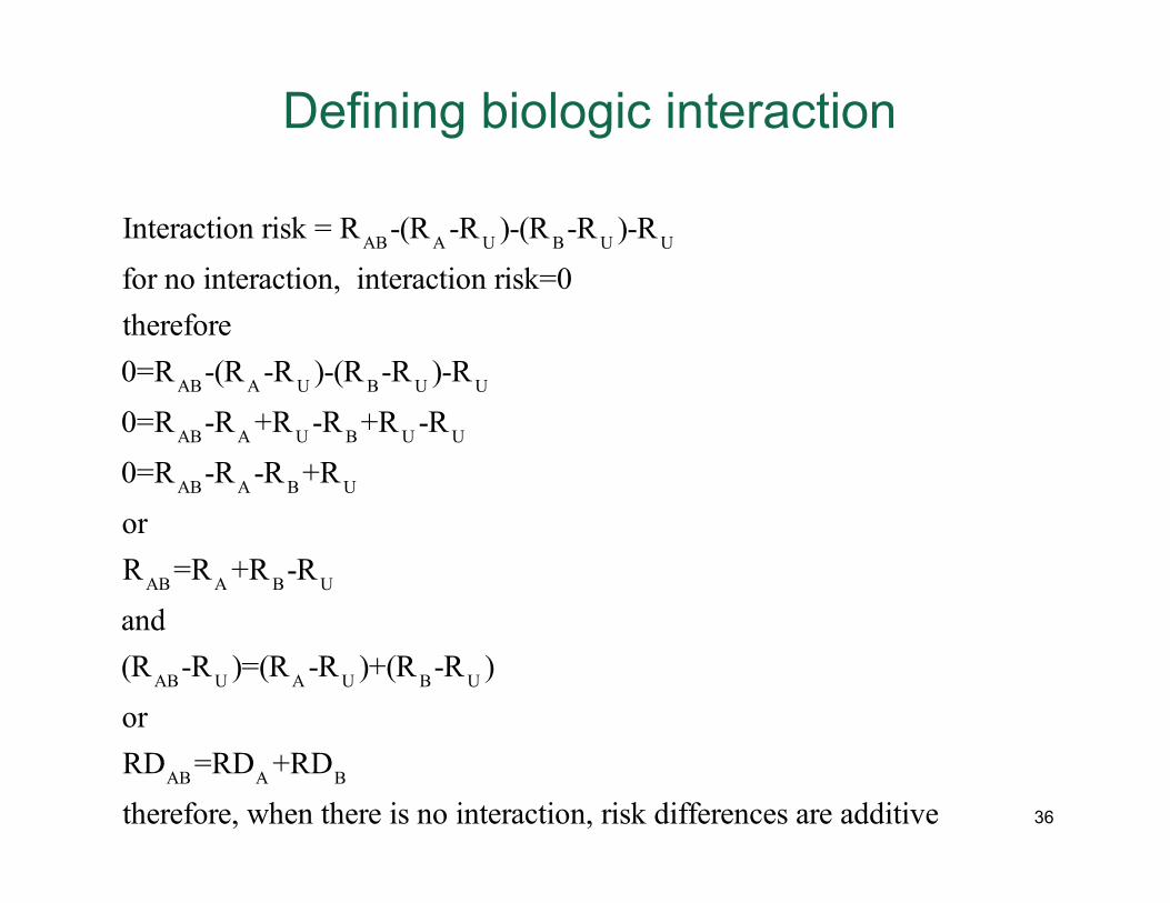
Interaction risk = RAB-(RA -RU )-(RB-RU )-RU
for no interaction, interaction risk=0therefore0=RAB-(RA -RU )-(RB-RU )-RU
0=RAB-RA +RU -RB +RU -RU
0=RAB-RA -RB +RU
orRAB =RA +RB-RU
and(RAB-RU )=(RA -RU )+(RB-RU )orRDAB =RDA +RDB
therefore, when there is no interaction, risk differences are additive 36
Continuing
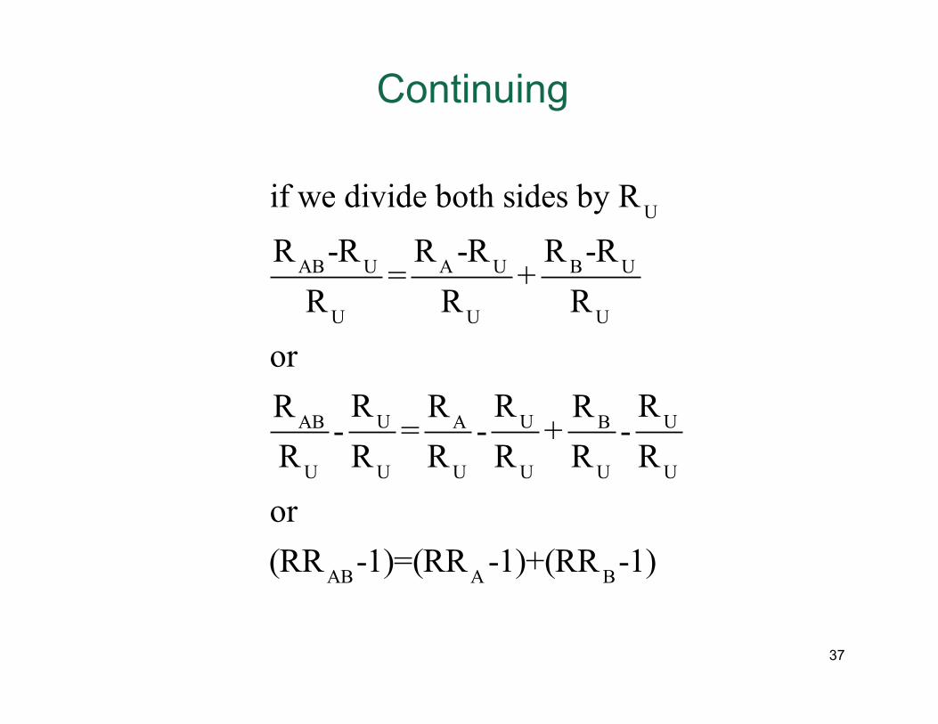
if we divide both sides by RU
RAB-RU
RU
=RA -RU
RU
+RB-RU
RU
orRAB
RU
-RU
RU
=RA
RU
-RU
RU
+RB
RU
-RU
RU
or(RRAB-1)=(RRA -1)+(RRB-1)
37
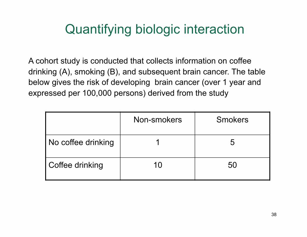
Quantifying biologic interaction
Non-smokers Smokers
No coffee drinking 1 5
Coffee drinking 10 50
A cohort study is conducted that collects information on coffee drinking (A), smoking (B), and subsequent brain cancer. The table below gives the risk of developing brain cancer (over 1 year and expressed per 100,000 persons) derived from the study
38
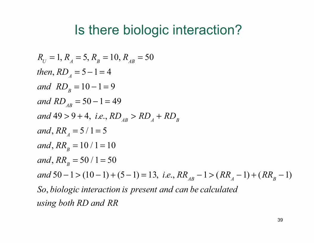
Is there biologic interaction?
RU = 1, RA = 5, RB = 10, RAB = 50then, RDA = 5−1= 4and RDB = 10 −1= 9and RDAB = 50 −1= 49and 49 > 9 + 4, i.e., RDAB > RDA + RDB
and , RRA = 5 / 1= 5and , RRB = 10 / 1= 10and , RRB = 50 / 1= 50and 50 −1> (10 −1) + (5−1) = 13, i.e., RRAB −1> (RRA −1) + (RRB −1)So, biologic interaction is present and can be calculatedusing both RD and RR
39
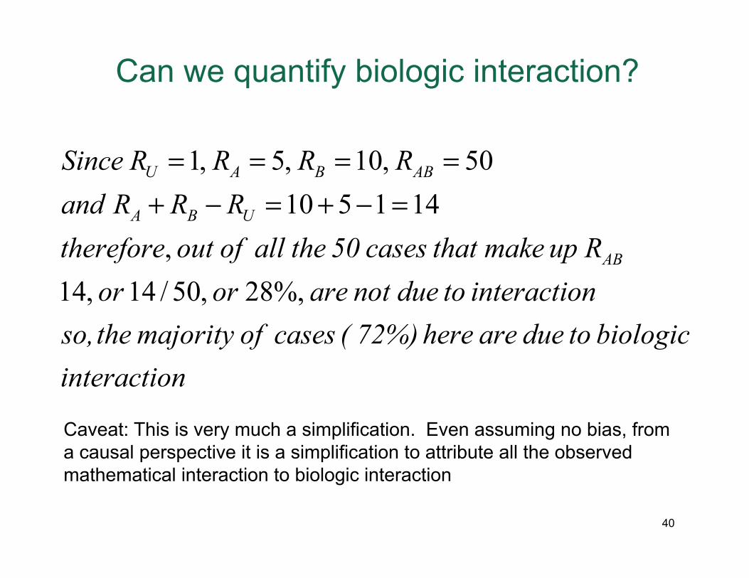
Can we quantify biologic interaction?
1, 5, 10, 5010 5 1 14
,14, 14 / 50, 28%,
U A B AB
A B U
AB
Since R R R Rand R R Rtherefore out of all the 50 cases that make up R
or or are not due to interactionso, the majority of cases ( 72%) here are due to
= = = =+ − = + − =
biologicinteraction
Caveat: This is very much a simplification. Even assuming no bias, from a causal perspective it is a simplification to attribute all the observed mathematical interaction to biologic interaction
40

Assess measure of association within strata
Are stratum specific measures same?
No Yes
Yes No
Confounding report measure
adjusted for confounding
Presumably no confounding or interaction
Report crude measure
Statistical interaction; report stratum specific measures
Crude measure=stratum specific?
Caveat: this is a simplification; stratum-
specific estimates of effect are almost never the same
and even if there is heterogeneity, sometimes it
is still appropriate to combine strata 41


