

Equalization of Doubly Selective Channels Using
Iterative and Recursive Methods
Thesis submitted to the University of Wales in candidature for the degree of
Doctor of Philosophy.
Sajid Ahmed
September 2005
Cardiff School of Engineering
University of Wales, Cardiff

2
DECLARATION
This work has not previously been accepted in substance for any degree and is not
being concurrently submitted in candidature for any degree.
Signed .............................................. (candidate)
Date ................................................
STATEMENT 1
This thesis is the result of my own investigation, except where otherwise stated. Other
sources are acknowledged by footnotes giving explicit reference. A bibliography is ap-
pended.
Signed .............................................. (candidate)
Date ................................................
STATEMENT 2
I hereby give consent for my thesis, if accepted, to be available for photocopying and
for inter-library loan, and for the title and summary to be made available to out side
organizations.
Signed .............................................. (candidate)
Date ................................................

3
To my parents for their prayers and assistance,
my brothers and sisters for their encouragement
and my wife for her continuous moral support.
4
Abstract
Novel iterative and recursive schemes for the equalization of time-varying fre-
quency selective channels are proposed. Such doubly selective channels are shown to
be common place in mobile communication systems, for example in second generation
systems based on time division multiple access (TDMA) and so-called beyond third
generation systems most probably utilizing orthogonal frequency division multiplex-
ing (OFDM).
A new maximum likelihood approach for the estimation of the complex multipath
gains (MGs) and the real Doppler spreads (DSs) of a parametrically modelled doubly
selective single input single output (SISO) channel is derived. Considerable com-
plexity reduction is achieved by exploiting the statistical properties of the training
sequence in a TDMA system. The Cramer-Rao lower bound for the resulting estima-
tor is derived and simulation studies are employed to confirm the statistical efficiency
of the scheme.
A similar estimation scheme is derived for the MGs and DSs in the context of a
multiple input multiple output (MIMO) TDMA system. A computationally efficient
recursive equalization scheme for both a SISO and MIMO TDMA system which ex-
ploits the estimated MGs and DSs is derived on the basis of repeated application of
the matrix inversion lemma. Bit error rate (BER) simulations confirm the advantage
of this scheme over equalizers which have limited knowledge of such parameters.
For OFDM transmission over a general random doubly selective SISO channel, the
time selectivity is mitigated with an innovative relatively low complexity iterative

5
method. Equalization is in effect split into two stages: one which exploits the spar-
sity in the associated channel convolution matrix and a second which performs a
posteriori detection of the frequency domain symbols. These two procedures interact
in an iterative manner, exchanging information between the time and frequency do-
mains. Simulation studies show that the performance of the scheme approaches the
matched filter bound when interleaving is also introduced to aid in decorrelation.
Finally, to overcome the peak to average power problem in conventional OFDM
transmission, the iterative approach is extended for single carrier with cyclic pre-
fix (SCCP) systems. The resulting scheme has particularly low complexity and is
shown by simulation to have robust performance.

6
Abbreviations and Acronyms
AML Approximate Maximum Likelihood
AMPS Advanced Mobile Phone System
AWGN Additive White Gaussian Noise
BER Bit Error Rate
BW Band Width
CCM Channel Convolution Matrix
CDMA Code Division Multiple Access
CIR Channel Impulse Response
CP Cyclic Prefix
CRLB Cramer-Rao Lower Bound
CSI Channel State Information
DFE Decision Feedback Equalizer
DQPSK Differential Quadrature Phase Shift Keying
DS Doppler Shift
EDGE Enhanced Data rates for GSM Evolution
ETACS European Total Access Communication System
FDD Frequency Division Duplex
FDE Frequency Domain Equalization
FDMA Frequency Division Multiple Access
FFT Fast Fourier Transform
FIR Finite Impulse Response
FIM Fisher Information Matrix
FO Frequency Offset
FRLS Fast-Recursive Least Squares

7
GMSK Gaussian Minimum Shift Keying
GPRS General Packet Radio Service
GSM Global System for Mobile Communications
HSCSD High Speed Circuit Switched Data
IBI Inter-block Interference
IC Interference Canceller
ICI Inter-Carrier-Interference
iff If and only if
IFFT Inverse Fast Fourier Transform
IS-95 Interim Standard-95
ISI Inter-Symbol-Interference
ITU International Telecommunication Union
LS Least-Squares
LTE Linear Transversal Equalizer
LTI Linear-Time-Invariant
LTV Linear-Time-Variant
OFDM Orthogonal Frequency Division Multiplexing
MCM Multi-Carrier Modulation
MFB Match Filter Bound
MIMO Multiple Input and Multiple Output
MIP Multipath Intensity Profile
MG Multipath Gain
MLE Maximum Likelihood Estimator
MMSE Minimum Mean Square Error
MS Mobile Station
MSE Mean Square Error
MVUE Minimum Variance Unbiased Estimator
NTT Nippon Telephone and Telegraph System
OFDM Orthogonal Frequency Division Multiplexing
PDC Personnel or Pacific Digital Cellular
8
PSK Phase Shift Keying
SCCP Single Carrier with Cyclic Prefix
SISO Single Input and Single Output
TD-SCDMA Time Division Synchronized Code Division Multiple Access
TDD Time Division Duplex
UMTS Universal Mobile Telecommunications System
UWB Ultra Wide Band
W-CDMA Wide band Code Division Multiple Access
WSSUS Wide Sense Stationary Uncorrelated Scattering
9
Operators
det(.) Determinant of a matrix
diag(.) Diagonal of matrix
E{.} Expectation
Re(.) Real Part of a Complex number
(.)T Transpose
(.)H Hermitian/Conjugate transposition
x Estimated sample
|.| Absolute value
‖.‖ Euclidean norm⊙
Schur-Hadamard Product∏
Interleaver
x Interleaved sample
O(N) Order N

10
Publications
Journal Papers
1. S. Ahmed, S. Lambotharan, A. Jakobsson and J. A. Chambers, “Parameter esti-
mation and equalization techniques for communication channels with multipath and
multiple frequency offsets,” IEEE Trans. Commun., vol. 53, pp. 219-223, Feb. 2005.
2. S. Ahmed, S. Lambotharan, A. Jakobsson and J. A. Chambers, “MIMO fre-
quency selective channels with multiple frequency offsets: estimation and detection
techniques,” IEE Proc. Commun., vol. 53, pp. 489- 494, Aug. 2005.
3. S. Ahmed, M. Sellathurai, S. Lambotharan and J. A. Chambers, “Low complexity
iterative method of equalization for single carrier with cyclic prefix in doubly selective
channels,” accepted for IEEE Signal Processing Letters.
4. S. Ahmed, M. Sellathurai, S. Lambotharan and J. A. Chambers, “Low complexity
iterative method of equalization for OFDM in doubly selective channels, ” submitted
to IEEE Trans. on Wireless Communications.
Conference Papers
1. S. Ahmed, S. Lambotharan, A. Jakobsson and J. A. Chambers, “Parameter esti-
mation and equalization techniques for MIMO frequency selective channels with mul-
tiple frequency offsets”, European Signal Processing Conference (EUSIPCO 2004),
Vienna, Austria.

11
2. S. Ahmed, J. A. Chambers and S. Lambotharan, “Frequency offset estimation tech-
nique for frequency selective channel with multiple frequency offsets in DS-CDMA”,
International Bhurban Conference on Applied Science and Technology (IBCAST 2004),
Bhurban, Pak.
3. S. Ahmed, M. Sellathurai, S. Lambotharan and J. A. Chambers, “Low complexity
iterative methods of equalization for OFDM,” European Signal Processing Confer-
ence (EUSIPCO 2005), Antalya, Turkey.
4. S. Ahmed, M. Sellathurai and J. A. Chambers, “Low complexity iterative method
of equalization for OFDM in time varying Channels,” accepted for 39th Asilomar
Conference on Signals, Systems and Computers, California, USA.

12
Statement of Originality
As far as the author knows the majority of the work presented in chapter 3 to 6
represents original contribution to the area of parameter estimation and equalization.
The originality is partially supported by four journal and four conference papers. The
most significant contributions are given below:-
1. In chapter 3, and [1] an Approximate Maximum Likelihood (AML) estimator
for a single input and single output multipath channel with distinct frequency offsets
is proposed. The AML estimator splits the L-dimensional maximization problem into
L one dimensional maximization problems. In this scenario to compensate for the ef-
fects of multiple frequency offsets, structural movements of the matrices are exploited
in the design of the Minimum Mean Squared Error (MMSE) equalizer, in particular,
repeated application of the matrix inversion lemma yields a low complexity equalizer.
2. In chapter 4, the parameter estimation and equalization of single input single
output channel is extended to Miltiple Input Multiple Output (MIMO) multipath
and distinct frequency offsets channels, the related work is presented in [2, 3].
3. In chapter 5 and [4–6], a new iterative equalization method for a doubly se-
lective Orthogonal Frequency Division Multiplexing (OFDM) channel is proposed.
The proposed method exploits the sparsity of the channel convolution matrix to de-
sign a general MMSE equalizer. The transmitted time domain samples are estimated
on the basis of interference cancellation. To cancel the interference the a posteriori
mean values are found from the a posteriori mean values of frequency domain symbols.

13
4. In chapter 6 and [7], iterative equalization of a single carrier cyclic prefix scheme
is proposed, which also exploits the sparsity of the channel convolution matrix to
find the general MMSE equalizer and estimator. In contrast to frequency domain
equalization of single carrier cyclic prefix, this algorithm benefits from not requiring
a fast Fourier and inverse fast Fourier transform at the receiver.
14
Acknowledgment
First of all, I would like to thank my respected supervisor Prof. J. A. Cham-
bers for his invaluable suggestions, guidance, patience and continuous encouragement
throughout my research work, without which it would not have been possible to ex-
ecute my research work.
I am also indebted to my co-supervisors Dr. S. Lambotharan and Dr. M. Sellathurai
for their discussions, criticism and suggestions in writing up my research work and
understanding the basics of my research work. I would especially like to express my
appreciation to Dr. S. Lambotharan, whose enthusiasm to discover novel equalization
techniques put me on the track for my PhD.
Special thanks to Dr. Andreas Jakobsson for his discussion on frequency offsets,
help in learning the type-setting package LaTex and advice on how to write research
papers.
I am very grateful to the Ministry of Science and Technology and Cardiff School
of Engineering for supporting me financially to complete my PhD.
I am most grateful to my research companions both in King’s College London and
Cardiff University, Dr. Wenwu Wang, Dr. Yi Hui, Dr. Maria Jafari, Dr. Cenk Toker,
Rab Nawaz, Shabbar Khan, Zhuo Zhang, Thomas Bowles, Qiang Yue, Li Zhang,
Yonggang Zhang, Min Jing, Zaid, Abdul Rehman, Ahmed Izzidien, Lay Teen, Clive
Cheong Took and Andrew Aubrey, for their great company and support.

CONTENTS
LIST OF FIGURES 18
LIST OF TABLES 22
1 INTRODUCTION 23
1.1 Channel Modelling 26
1.1.1 Sinusoidal time-varying channel 27
1.1.2 A general time-varying channel 29
1.2 Channel Classification 32
1.3 Outline of the Thesis 33
2 PARAMETER ESTIMATION AND EQUALIZATION 37
2.1 Basic Baseband Model of a Communication System 37
2.2 Equalization Techniques 40
2.2.1 Linear Transversal Equalization 41
2.2.2 Non-Linear Equalization 42
2.2.3 Iterative Equalization based on Interference Cancellation 45
2.2.4 Adaptive Equalization 47
2.3 Cramer Rao Lower Bound 48
2.4 Channel Parameter Estimation 52
2.4.1 Supervised Parameter Estimation 52
15
16
2.5 FO Estimation 58
2.5.1 Frequency domain transformation 58
2.5.2 Sub-space based FO estimation 58
2.5.3 Un-supervised Parameter Estimation 59
2.6 Summary 60
3 PARAMETER ESTIMATION AND EQUALIZATION IN SISO
WITH FREQUENCY OFFSETS 61
3.1 Problem statement 63
3.2 Estimation of multipath gains and frequency offsets 65
3.3 Numerical Example for Variance of Estimators 67
3.4 MMSE equalizer design 70
3.4.1 Equalizer for channels without FOs 70
3.4.2 Equalizer for channels with frequency offsets 71
3.5 Simulations 73
3.6 Summary 76
3.7 Appendices 3 77
4 PARAMETER ESTIMATION AND EQUALIZATION IN MIMO
WITH FREQUENCY OFFSETS 79
4.1 Problem Statement 80
4.2 Estimation of Multipath Gains and Frequency Offsets 82
4.3 Numerical Example for the Variance of the Estimators 84
4.4 A MIMO Recursive MMSE Equalizer Design 87
4.5 Simulation 91
4.6 Summary 93
4.7 Appendices 4 94
5 ITERATIVE EQUALIZATION FOR OFDM SCHEMES 99
5.1 A Brief Overview of an OFDM System 101

17
5.2 Problem Statement 104
5.3 Equalization 106
5.3.1 MMSE Equalization 107
5.3.2 Iterative Algorithm 109
5.4 Complexity of the Algorithm 112
5.5 Simulation 114
5.6 Summary 120
5.7 Appendices 5 121
6 ITERATIVE EQUALIZATION FOR A SINGLE CARRIER WITH
CYCLIC PREFIX SCHEME 123
6.1 A Brief Overview of the SCCP System 124
6.2 Problem Statement 125
6.3 Symbol Estimation 128
6.3.1 MMSE Equalizer 128
6.3.2 Iterative Algorithm 129
6.4 Complexity of the Algorithm 133
6.4.1 Linear Time Variant Channel 133
6.4.2 Linear Time Invariant Channel 134
6.5 Simulation 134
6.6 Summary 139
7 CONCLUSION AND FUTURE WORK 140
7.1 Conclusion 140
7.2 Future Work 143
BIBLIOGRAPHY 145

List of Figures
1.1 BER performance comparison of two receivers; one is assuming identi-
cal DS from each path and the second is accounting for multiple DSs
from each multipath. For both simulations the length of the channel
is kept equal to 2 and a 10 taps equalizer is used. 29
1.2 Time variations in the amplitudes of two multipaths of a Rayleigh
fading channel. 31
1.3 Time variations in the amplitudes of two multipaths of a Rayleigh
fading channel based on Jakes’ model. 31
1.4 Multipath intensity profile and corresponding frequency domain rep-
resentation. 32
2.1 Baseband model of a digital communication system, consisting of the
transmitter, channel and equalizer (receiver). 38
2.2 Linear Transversal Equalizer 41
2.3 A basic structure of a DFE with forward and feedback filters. 44
2.4 Frame structure of GSM communications. 53
3.1 Comparison of the variance of the estimates of h0 and h1 with the CRLB 69
3.2 Comparison of the variance of the estimates of f0 and f1 with the CRLB 69
3.3 Bit error rate performance for MMSE equalizers with and without FO
estimation, and a decision directed adaptive equalizer 75
18

LIST OF FIGURES 19
3.4 Bit error rate performance of MMSE equalizers for a GSM system 75
4.1 Comparison of the variance of the estimates of channel gains (dashed
line) with the corresponding CRLB (solid line). 86
4.2 Comparison of the variance of the estimates of FOs (dashed line) with
the corresponding CRLB (solid line). 86
4.3 A two transmitter and three receiver MIMO transmitter and receiver
baseband system. 87
4.4 Bit error rate performance comparison of the proposed scheme account-
ing for FOs in the equalizer design with the conventional equalizer
scheme ignoring the FOs in the equalizer design. For bench mark the
simulation result of a conventional scheme when there is no FO in the
channel is also shown. 92
5.1 Time and frequency response of an 8 carrier OFDM system. Subplots
c1 to c8 show the subcarriers, f1 to f8 show the corresponding mag-
nitudes of the frequency spectrum occupied by each station and the
bottom two show the sum of time waveforms and frequency spectrum. 102
5.2 A basic baseband OFDM system, transmitting subsequent blocks of N
complex data and the receiver removing the cyclic prefix and perform-
ing frequency domain equalization. 103
5.3 A basic baseband OFDM system, transmitting subsequent blocks of N
complex data and an iterative detection of the transmitted data. 104
5.4 Diagonal like structure of the channel convolution matrix, H, showing
the sparsity. The dots represent the non-zero elements. 107
5.5 Bit-error-rate performance of the MMSE-iterative algorithm after dif-
ferent numbers of iterations at DS of 0.01. 116
5.6 Bit-error-rate performance of the MMSE-iterative algorithm after dif-
ferent numbers of iterations at DS of 0.05. 116

LIST OF FIGURES 20
5.7 BER performance comparison of the MMSE-iterative algorithm, after
five iterations and at different DSs, with the L-MMSE equalizer and
MFB. 117
5.8 SER performance comparison of the MMSE-iterative algorithm, after
five iterations and at different DSs, with the L-MMSE equalizer and
MFB. 117
5.9 BER performance comparison of the MMSE-iterative algorithm, after
five iterations and at different DSs, with the L-MMSE equalizer and
MFB. 118
5.10 SER performance comparison of the MMSE-iterative algorithm, after
five iterations and at different DSs, with the L-MMSE equalizer and
MFB. 118
5.11 Bit-error-rate performance using an MMSE-iterative algorithm after
five iterations at different DSs for different number of carriers in an
OFDM block. 119
6.1 A basic baseband SCCP scheme, transmitting subsequent blocks of N
data symbols and the receiver is performing frequency domain equal-
ization, where L is the support of channel. 125
6.2 A baseband iterative SCCP system, transmitting subsequent blocks of
N data symbols and the receiver is performing iterative time domain
equalization. 126
6.3 BER performance of the iterative algorithm after different number of
iterations at slow fading fd = 0.001.The number of symbols in a SCCP
block is 32. 136
6.4 BER performance of the iterative algorithm after different number of
iterations at fast fading fd = 0.05. The number of symbols in a SCCP
block is 32. 136

LIST OF FIGURES 21
6.5 Bit error rate performance comparison of the proposed iterative al-
gorithm after five iterations with the L-MMSE equalizer and MFB at
different DSs. The number of symbols in one block is 32 and the length
of the channel is 4. 137
6.6 Symbol error rate performance comparison of the proposed iterative
algorithm after five iterations with the L-MMSE equalizer and MFB
at different DSs. The number of symbols in one block is 32 and the
length of the channel is 4. 137
6.7 BER performance comparison of the proposed iterative algorithm after
five iterations with the L-MMSE equalizer and MFB at different DSs.
The number of symbols in one block is 64 and the length of the channel
is 4. 138
6.8 BER performance comparison of the proposed iterative algorithm for
an LTI channel after five iterations with the FDE and MFB. In both
equalizations, the number of symbols in one block is 32 and the length
of the channel is 4. 138

List of Tables
1.1 Air interfaces and spectrum allocation in first generation mobile systems. 23
1.2 Air interfaces and spectrum allocation for second generation mobile
systems. 24
1.3 Expected air interfaces and spectrum allocation for third generation
mobile systems. 26
5.1 MMSE-Iterative algorithm for OFDM 113
6.1 MMSE-Iterative algorithm for SCCP 133
22
Chapter 1
INTRODUCTION
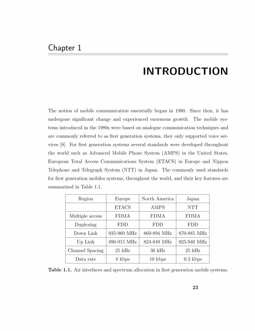
The notion of mobile communication essentially began in 1980. Since then, it has
undergone significant change and experienced enormous growth. The mobile sys-
tems introduced in the 1980s were based on analogue communication techniques and
are commonly referred to as first generation systems, they only supported voice ser-
vices [8]. For first generation systems several standards were developed throughout
the world such as Advanced Mobile Phone System (AMPS) in the United States,
European Total Access Communications System (ETACS) in Europe and Nippon
Telephone and Telegraph System (NTT) in Japan. The commonly used standards
for first generation mobiles systems, throughout the world, and their key features are
summarized in Table 1.1.
Region Europe North America Japan
ETACS AMPS NTT
Multiple access FDMA FDMA FDMA
Duplexing FDD FDD FDD
Down Link 935-960 MHz 869-894 MHz 870-885 MHz
Up Link 890-915 MHz 824-849 MHz 925-940 MHz
Channel Spacing 25 kHz 30 kHz 25 kHz
Data rate 8 kbps 10 kbps 0.3 kbps
Table 1.1. Air interfaces and spectrum allocation in first generation mobile systems.
23

24
In the 1990s digital transmission techniques were introduced and formed the second
generation systems. They provided increased spectrum efficiency and higher quality of
voice services than the first generation systems together with better data services [9].
The digital standards currently in use, such as Global System for Mobile commu-
nications (GSM) in Europe, Interim Standard-95 (IS-95) in the United States and
Personnel or Pacific Digital Cellular (PDC) in Japan, are second generation systems.
The most common standards used for second generation mobile systems in the world
and their key features are summarized in Table 1.2.
Region Europe North America North America Japan
GSM TDMA (IS-54/136) IS-95 PDC
Multiple access TDMA TDMA CDMA TDMA
Duplexing FDD FDD FDD FDD
Modulation GMSK π/4 DQPSK QPSK/OQPSK π/4 DQPSK
Down-link 935-960 MHz 869-894 MHz 869-894 MHz 810-826 MHz
Up-link 890-915 MHz 824-849 MHz 824-849 MHz 940-956 MHz
Channel spacing 200 kHz 30 kHz 1,250 kHz 25 kHz
Data/Chip rate 270.833 kbps 48.6 kbps 1.2288 Mcps 42 kbps
Table 1.2. Air interfaces and spectrum allocation for second generation mobile
systems.
The initial second generation systems were originally designed for the delivery of only
high quality voice services and their data handling capabilities were limited to several
tens of kbps [10]. Therefore, for high data rates and more advance services, such as
packet switched data, second generation systems were further upgraded and referred
to as 2.5 generation systems. The three upgrade options for GSM include; Enhanced
Data Rate for GSM Evolution (EDGE) that can provide data rates up to 500kbps
within a GSM carrier spacing of 200kHz, General Packet Radio Services (GPRS), as
the name implies, is a packet switch technique and High Speed Circuit Switched Data
25
(HSCSD), which is a circuit switched technique that allows a single mobile user to
use consecutive time slots in the GSM standard for high data rate applications [11].
EDGE and GPRS are also the upgrade options for IS-136, while the cdma2000 stan-
dard is the upgrade option for IS-95. [12].
In the 21st century, wireless mobile telephony is rapidly growing and providing new
and improved multimedia services. High quality images and video will be transmitted
and received; moreover, mobile telephony provides access to the web with high data
rate requiring asymmetric access. Emerging requirements for high data rate services
and better spectrum efficiency are the main drivers identified for the third gener-
ation mobile communication systems [9, 13]. The International Telecommunication
Union (ITU) describes third generation networks as IMT-2000 and prescribes wide-
band CDMA as the air interface. The main objectives of the IMT-2000 standard are
summarized as [11,14]
• Data rate of 344 kbps for vehicular environment
• Data rate of 2 Mbps for indoor environment
• Higher spectrum efficiency as compared to existing system
• High flexibility to introduce new services
Today’s research focuses on beyond third generation or fourth generation wireless
systems, where mobile users may use portable computers. In the first phase the
operating frequencies of fourth generation systems may be around 5.8GHz, and are
likely to support [15]
• 2 Mbps for moving vehicles, and
• 2-600 Mbps for low mobility systems
This is the background to the evolution of mobile communication systems since 1980.
To meet the demands for increased data rate services and improved spectrum effi-

Section 1.1. Channel Modelling 26
Region Europe North America China
UMTS CDMA-2000 TD-SCDMA
Multiple access W-CDMA MC-CDMA CDMA
Duplexing FDD/TDD FDD TDD
Data Rate 2Mbps 2Mbps 2Mbps
Downlink 2110-2170MHz 1930-1990MHz 2010-2025MHz
Uplink 1920-1980MHz 1850-1910MHz 2010-2025MHz
Channel spacing 5MHz 5MHz 5MHz
Chip Rate 3.84Mcps 3.6864Mcps 1.28Mcps
Table 1.3. Expected air interfaces and spectrum allocation for third generation
mobile systems.
ciency advanced digital signal processing techniques must be exploited at the physical
layer [16], the heart of which is the radio channel between the transmitter and receiver.
1.1 Channel Modelling
In wireless mobile systems, communication is not normally line of sight, particularly
in an urban environment; instead, the received signal consists of a large number of
reflected, refracted and scattered waves. Therefore, the signal travels from the trans-
mitter to receiver via more than one path. Due to this multipath propagation, the
transmitted signal arrives at the receiver at different time instances and with dif-
ferent amplitudes that may give rise to Inter-Symbol-Interference (ISI) [17]. An ISI
producing channel is termed frequency selective. ISI is a fundamental limiting factor
in the performance of high data rate communication, within the physical layer of a
mobile communication system. If the channel is not changing significantly within the
observation interval of time then the effects of ISI can be compensated for relatively
easily by using an equalizer. In the noiseless case, an equalizer is designed such that
the convolution of its impulse response with the channel impulse response should ide-
Section 1.1. Channel Modelling 27
ally be a Kronecker delta function [17]. Such an equalizer may require knowledge of
the channel impulse response, which is not usually available. Hence, to estimate the
channel impulse response, the transmitter is generally required to send training data,
already known at the receiver. Indirect equalization techniques, such as adaptive do
not require CSI, can also be employed. These techniques learn the channel or its
inverse without estimating it [18].
On the other hand, if the frequency selective channel is time-varying (also called time
selective), it is referred to as a doubly selective channel. Time selectivity of the chan-
nel degrades the Bit-Error-Rate (BER) performance and increases the computational
complexity of conventional receivers [1, 19]. However, time selectivity of the channel
can be exploited to obtain time diversity benefit.
Therefore, the design of a relatively low complexity receiver that can provide signif-
icant improvement in BER performance over a conventional receiver in a frequency
selective environment is the main motivation for this thesis. The causes of time
variations in the channel are next discussed.
1.1.1 Sinusoidal time-varying channel
As previously discussed, from first generation to beyond third generation, the require-
ment for high data rates is continuously increasing. With the increase in data rate
the operating frequency is also increasing. Mobility in the systems, at high operating
frequencies yields significant Doppler Shifts (DSs). Therefore, even if in a given inter-
val of time the channel is not changing due to mobility, the DS may introduce time
selectivity in the channel. Consequently, the assumption that the channel is constant,
in a given interval of time, does not hold true and affect the BER performance of the
receiver. In order to improve the BER performance of the receiver, the effects of the
time selectivity of the channel due to DS must be cancelled. In most of the available
literature [20–23], it is commonly considered that all multipaths have identical DSs
and can be compensated for relatively easily prior to MLSE or adaptive equalization.

Section 1.1. Channel Modelling 28
However, the DS is defined as
fd =fcvr
ccos θ (1.1.1)
where vr, is the speed of the mobile station (MS) in m/s, fc is the carrier frequency in
Hz, c is the velocity of light in m/s and θ is the angle of arrival in radians. This equa-
tion shows that if the relative speed between the base station and MS is constant, then
the DS will be a function of the angle of arrival. Therefore, when the DS is significant
it is necessary to account for it from each angle of arrival or multipath, which is one
of the main motivations of this thesis. For example, consider a mobile user in a fast
moving vehicle with a speed of approximately 250 km/h and a carrier frequency of 4
GHz. The DS at the base station for an arrival angle of zero degrees, is approximately
1 kHz, whilst for an arrival angle of 60 degrees becomes 0.5kHz. This results in phase
deviations of approximately 18 and 9 degrees respectively for both arrival angles, in
every bit period, for a bit rate of 20 kbit/s, and distinct sinusoidal time variations into
each multipath of the channel. In this scenario, it is difficult to compensate for the
effects of DSs prior to equalization and that must be accounted for in equalizer design.
Numerical Example: In order to examine the benefits of accounting for the distinct
DSs in equalizer design, the above mentioned scenario is simulated. In the first case,
the receiver assumes the same DS from each multipath and cancels the effects of DS
prior to equalization, which is a general type of equalization for frequency offset com-
pensation. In the second case, the receiver assumes distinct DSs from each multipath
and accounts for them in the equalizer design. The BER performances of both cases
are depicted in Figure 1.1. It can be noted that in the equalizer design accounting
for distinct DSs from each multipath a better performance as compared to assuming
identical DSs from each multipath is obtained. For example, at a fixed BER of 10−3,
a 2 dB improvement in SNR is required by the receiver assuming a single DS.

Section 1.1. Channel Modelling 29
0 2 4 6 8 10 12 1410
−6
10−5
10−4
10−3
10−2
10−1
SNR
BE
R
Single frequency correctionBoth frequency corrections
Figure 1.1. BER performance comparison of two receivers; one is assuming identical
DS from each path and the second is accounting for multiple DSs from each multipath.
For both simulations the length of the channel is kept equal to 2 and a 10 taps equalizer
is used.
1.1.2 A general time-varying channel
In wireless mobile communications the channel is not stationary at all times, it may
vary with respect to time. In wireless and wire-line communications data are trans-
mitted in frames and it is assumed that the channel is not changing during one
frame at least [17]. But, sometimes the channel does not remain constant even in
one frame. Therefore, to describe time varying nature of the channels a more general
time-varying channel is modelled. Wide Sense Stationary and Uncorrelated Scattering
(WSSUS) model is the most commonly used channel model in wireless communica-
tions [17, 24, 25]. In the WSSUS model the channel is characterized by its delay (or
multipath) power spectrum and the scattering function.
When an impulse is transmitted over a multipath channel the received signal is a train
of impulses. The range of locations of impulses with sufficient strength reveals the

Section 1.1. Channel Modelling 30
spreading of the channel. If the channel is time-varying then the complex strength of
each impulse in the train will be time-varying in a random manner. For the WSSUS
model the impulse response can be written as
h(n; l) =L−1∑
p=0
h(n; lp)δ(l − lp), (1.1.2)
where h(n, l) denotes the complex gain of the lth path at time n. L and δ(.) denote
respectively the total number of paths, and the Kronecker delta function. Moreover,
l ǫ {lo l1 · · · lL−1}, and lo < l1 < · · · < lL−1. The auto-correlation of the channel is
given by
E{h(n1; l1)h∗(n2; l2)} = r
hh(n1 − n2; l1 − l2) (1.1.3)
where (.)∗ denotes the complex conjugate operator. Since, the multipaths are uncor-
related
E{h(n1; l1)h∗(n2; l2)} = r
hh(n1 − n2; l1)δ(l1 − l2), (1.1.4)
and can be decomposed into time and multipath auto-correlation functions as,
rhh
(n1 − n2; l) = rtt(n1 − n2)rpp
(l), (1.1.5)
where rtt(n1−n2) and r
pp(l) are respectively the auto-correlation of the lth path with
respect to time and the auto-correlation of the channel (assuming time stationarity)
with respect to multipath which is also called the Multipath Intensity Profile (MIP)
[17].
Example: For a Rayleigh fading channel, h(n, l) is a white Gaussian random variable
with zero mean and σ2l |l=0,1,...,L−1 is the variance of the lth multipath. Moreover,
h(n, l)|l=0,1,...,L−1 are independent. Therefore, for a Rayleigh fading channel
rtt(n1 − n2) = 0 if n1 − n2 6= 0 (1.1.6)
= 1 if n1 − n2 = 0 (1.1.7)
and rpp
(l) = σ2l . (1.1.8)

Section 1.1. Channel Modelling 31
050100150200−35
−30
−25
−20
−15
−10
−5
0
5
10
15
Time Index n
Cha
nnel
taps
am
plitu
des
(dB
) h(n,0)h(n,1)
Figure 1.2. Time variations in the amplitudes of two multipaths of a Rayleigh fading
channel.
0 50 100 150 200−30
−25
−20
−15
−10
−5
0
5
10
Time Index n
Cha
nnel
taps
am
plitu
des(
dB)
fd = 0.05
h(n,0)h(n,1)
Figure 1.3. Time variations in the amplitudes of two multipaths of a Rayleigh fading
channel based on Jakes’ model.

Section 1.2. Channel Classification 32
If the coefficients h(n, l) are taken from the classical Jakes’ model [26] then
rtt(n1 − n2) = Jo [2πfd(n1 − n2)] if n1 − n2 6= 0 (1.1.9)
= 1 if n1 − n2 = 0 (1.1.10)
and rpp
(l) = σ2l ,
where Jo(·) denotes the zeroth order Bessel function of the first kind and fd is the
normalized DS. In Figures 1.2 and 1.3, the envelopes of a two multipath Rayleigh
fading and a Rayleigh fading channel based on Jakes’ model are plotted with respect
to time. These plots confirm the highly time-varying nature of such channels. The
time width for which the MIP is not diminishingly small defines the spreading of the
channel. If the spreading of the channel is Ts seconds then the coherence bandwidth
of the channel can be defined as [27],
(BW )h =1
Ts
. (1.1.11)
The relationship between the MIP, rpp(l), and its frequency spectrum, Rpp(f), is
shown in Figure 1.4
l f
Fourier transform
Inverse Fourier transform
r pp ( l ) |R pp ( f )|
0 0
Figure 1.4. Multipath intensity profile and corresponding frequency domain repre-
sentation.
1.2 Channel Classification
The MIP helps to describe the nature of the channel. A channel is said to be frequency
flat or non selective if within the bandwidth, BW , occupied by the transmitted signal

Section 1.3. Outline of the Thesis 33
the amplitude response of Rpp(f) is constant. In the time domain, it can be said that
the spreading time, Ts, is less than the symbol period, T . Flat fading does not
introduce ISI. Therefore, such a channel satisfies
Ts << T. (1.2.1)
On the other hand, a channel is said to be frequency selective if within the bandwidth,
BW , occupied by the transmitted signal, the amplitude response Rpp(f) is not flat for
the entire bandwidth of the transmitted signal. Hence, each frequency component of
the signal is amplified and phase shifted differently. Here, the multipath propagation
spreads the transmitted signal over an interval of time which is longer than the symbol
period, which can cause ISI. For frequency selective fading the channel satisfies
Ts >> T (1.2.2)
i.e. the spreading of one symbol by the channel overlaps its neighbors.
1.3 Outline of the Thesis
Overview: This thesis proposes relatively low complexity equalization methods for
time-varying frequency selective channels for communication systems that are based
on Time Division Multiple Access (TDMA), Multiple Input Multiple Output (MIMO),
Orthogonal Frequency Division Multiplexing (OFDM) and Single Carrier with Cyclic
Prefix (SCCP) technologies. In the first two contribution chapters (chapters 3 and 4),
the time variations in the multipaths of the channels are sinusoidal, while, in last two
contribution chapters (chapters 3 and 4), a more general and realistic time-varying
multipath channel is considered. This evolution corresponds to my period of research
study. The following sub-sections review briefly what can be found in each of the five
contribution chapters.
Chapter 3 studies parameter estimation and equalization for a Single Input Single
Output (SISO), TDMA based communication system, such as GSM, where it is as-
sumed that each multipath of the channel has distinct DS and thereby makes the

Section 1.3. Outline of the Thesis 34
problem different from the identical DS problem. Here, unlike the identical DS prob-
lem [20,28,29], the distinct DSs cannot be compensated for prior to equalization and
must be accounted for in equalization. In order to design an equalizer the complex
Multipath Gains (MGs) and DSs are required. Presence of the distinct DSs converts
the estimation of these parameters into a complicated L+1 dimensional optimization
problem, where L is the length of the channel. Therefore, in order to estimate the
MGs and DSs, the correlation property of the transmitted training signal sequence is
exploited which thereby splits the L + 1 dimensional estimation problem into L + 1
one-dimensional problems. A maximum likelihood estimation approach is used to find
the complex MGs and DSs. Moreover, to estimate the DSs the proposed algorithm
does not require explicit knowledge of the MGs of the channel but requires knowledge
of the support L of the channel. Then, to assess the performances of the proposed
estimators the benchmark Cramer Rao lower bound (CRLB) for DSs and MGs [30]
is derived.
As distinct DSs introduce time selectivity into the channel, adaptive and blind adap-
tive equalizers yield poor BER performance as the equalizer taps need to be up-
dated after every symbol interval. Further, it has been shown that the conventional
minimum mean square error (MMSE) equalizer is computationally cumbersome as
the effective channel convolution matrix (CCM) changes deterministically between
symbols, due to the multiple DSs. By exploiting the structural property of these
variations, and using multiple application of the matrix inversion lemma, a compu-
tationally efficient recursive algorithm for the equalizer design is proposed.
Chapter 4 extends the work presented in chapter 3 to MIMO frequency selective
channels with each multipath having distinct DS. The MIMO technology uses mul-
tiple antennas at both the transmit and the receive sides to obtain spatial diversity.
Recent research in communication theory has shown that large gains in diversity, ca-
pacity and reliability of communications over wireless channels could be achieved by
exploiting such spatial diversity and will play a key role in future high rate wireless

Section 1.3. Outline of the Thesis 35
communications provided there is rich scattering environment [31,32]. The parameter
estimation for flat fading channels in MIMO is studied in [33]. In this chapter the
parameters in a MIMO system, allowing for a frequency selective channel between
each transmit and receive antenna and each multipath, possibly having distinct DSs,
are estimated. The training signals transmitted by all the antennas are assumed to be
spatially and temporally uncorrelated. Therefore, by exploiting this property, MGs
and DSs are estimated. In order to assess the performances of the estimators the
benchmark CRLB is derived and used to compare the performances of the estima-
tors.
Again, as in chapter 3, by exploiting the structural property of the variations in the
CCM in this case, the computationally efficient recursive algorithm reduces the di-
mension of the matrix to find the inverse of the matrix that is needed to find the
equalizer coefficient values from nRM × nRM to nR × nR, where nR is the number of
receive antennas and M is the number of equalizer taps, as addressed in [2, 3].
Chapter 5 studies the equalization of a general time-varying channel for an OFDM
based system. Here in contrast to previous work, each multipath of the channel is
randomly time varying. For this scenario the approach discussed in chapters 3 to 4
can not be applied, since the CCM does not change deterministically. To combat the
effects of time selectivity of the channel in an OFDM system, Schniter in [19] pre-
processed the received signal by multiplying with window coefficients that render the
Inter-Carrier-Interference (ICI) response sparse, and thereby squeeze the significant
coefficients into the 2D+ 1 central diagonals of an ICI matrix. Here, it is found that
D = fdN +1, where fd is the DS in the carrier frequency and N is the number of car-
riers used to transmit an OFDM symbol. The complexity of this algorithm increases
as the DS increases. In contrast to this work, examining the time domain model of
the received OFDM signal reveals that the CCM is already sparse and has similar
structure to that after preprocessing of the received samples in [19]. In this case, the
number of non-zero elements in a row depends on the length of channel taps L, which
Section 1.3. Outline of the Thesis 36
for a wireless channel is typically small, for example 5. Therefore, in this chapter,
a new low complexity iterative method is addressed to compensate for the effects of
time selectivity of the channel. The method splits the equalization into two stages.
The first stage exploits the sparsity present in the CCM to estimate the time domain
transmitted samples and the second stage performs the a posteriori detection of the
frequency domain symbols. Both the stages exchange their information iteratively.
The performance of the algorithm is compared with the match filter bound.
Chapter 6 studies the equalization of a single carrier with cyclic prefix (SCCP)
scheme in a time varying frequency selective channel. A SCCP is an alternative to
OFDM. OFDM is an attractive technique for transmission over frequency selective
channels since it allows low complexity channel equalization at the receiver. However,
OFDM requires an expensive and efficient transmitter amplifier at the front end, due
to high peak-to-average power ratio (PAPR). Single carrier with cyclic prefix (SCCP)
is a closely related transmission scheme that possesses most of the benefits of OFDM
but does not require an expensive linear amplifier that can operate linearly over a
wide range of signal amplitudes. Although similar to OFDM, in a time invariant mul-
tipath environment an SCCP system is very robust, it is sensitive to the time selective
fading characteristics of the wireless channel. Time selectivity of the channel disturbs
the orthogonality of the channel matrix, thereby degrading the system performance
significantly and increasing the computational complexity of the receiver. On the
other hand, time selectivity introduces temporal diversity that can be exploited to
improve the performance. In this chapter, working with time domain samples, a low
complexity iterative algorithm is proposed to compensate for the effects of time selec-
tivity of the channel, which exploits the sparsity present in the CCM and a Maximum
a Posteriori (MAP) detection in an iterative fashion, as in [7].
Finally, in chapter Chapter 7 conclusions are drawn and future research directions
are suggested.
Throughout the thesis, MATLAB is used to simulate all the problems.

Chapter 2
PARAMETER ESTIMATION AND
EQUALIZATION
In many radio communication systems such as wireless mobile, wire-line telephone and
optical transmission there may be more than one path, also called multipaths, between
the transmitter and the receiver. In mobile telephony these multipaths may be due
to the reflections and refractions from the buildings and other obstacles between the
transmitter and receiver [17]. In wireline telephony that may be due to the dispersive
nature of the wires [34, 35]. Multipaths may give rise to ISI, which limits high data
rate transmission. Therefore, in a multipath environment to detect correctly the
transmitted data, generally, a complex equalizer is designed that sometimes requires
the Channel Impulse Response (CIR) i.e. the complex channel MGs. In order to
estimate the CIR, generally, a training sequence is embedded in the transmitted
signal sequence. In this chapter, a brief background to the technology of equalization
and parameter estimation is presented.
2.1 Basic Baseband Model of a Communication System
Almost all baseband digital communication systems consist of three basic building
blocks, the transmitter, the channel and the equalizer (receiver) as shown in Figure
2.1. In the figure, x(n) is the transmitted symbol, {h(n)} is the MGs sequence,
v(n) is the additive noise sample, r(n) is the received sample, {w(n)} are equalizer
37

Section 2.1. Basic Baseband Model of a Communication System 38
coefficients, x(n) is the estimated signal after equalization and n is the discrete time
index.
Channel
{ h(n)}Equalizer
{ w(n)}+x(n)
v(n)
x (n)r(n)Transmitter
Figure 2.1. Baseband model of a digital communication system, consisting of the
transmitter, channel and equalizer (receiver).
In the basic baseband model of a digital communication system, the transmitter is one
of the most important parts of a digital communication system. The main function
of the transmitter is to convert the raw data into an appropriate form suitable for
transmission, e.g., the voice signal is sampled and encoded into binary signals to
transmit. The original band of frequencies occupied by the encoded binary signals is
called a baseband signal. The baseband signal has wide frequency spectrum centered
at zero frequency, which is bandlimited before transmission with a filter called a
transmit filter. Usually the binary signals contain low frequencies, which are difficult
to propagate. Hence, signals centered around higher frequencies are preferred. The
second function of the transmitter is therefore to shift the frequency spectrum of
the bandlimited signal to some higher frequency centered at fc called the carrier
frequency. To shift the frequency spectrum to a higher frequency, the bandlimited
signal is multiplied by the high frequency sinusoidal signal of frequency fc [17]. The
output signal is termed as the passband and the mapping of the baseband signal into
the passband signal is called modulation.
The transmitted signal passes through the channel that can be considered as a Finite
Impulse Response (FIR) filter and arrives at the receiver. The received signal is again
passed through a filter called the receive filter matched to the frequency band of the
transmitter. In general, the effects of the transmit filter, the transmission medium
and the receive filter are included in the channel model h(n) with finite time support.

Section 2.1. Basic Baseband Model of a Communication System 39
Therefore, if the support of the modelled channel is L and the sampling rate at the
receiver is equal to the symbol transmission rate then the received signal can be
written as
r(n) =L−1∑
l=0
h(l)x(n− l) + v(n) (2.1.1)
Before proceeding, the following assumptions are made that are imposed throughout
this thesis.
• The transmitted symbols {x(n)} are independently and identically distributed
(i.i.d).
• The additive noise samples {v(n)} are zero mean white circularly Gaussian with
variance σ2v .
• The channel is an FIR filter of support L.
Let the multipath component h(m) possess the highest relative amplitude in the
sequence {h(n)}, this multipath is termed as main multipath, multipaths before and
after the main multipath are respectively called pre- and post-cursors. The energy
of the wanted signal is conveyed mainly by the contribution of the main path. In
addition to that the received signal is also contributed to by the convolution of pre-
and post-cursors. Therefore, the received signal in (2.1.1) can be written as
r(n) = h(m)x(n−m) +L−1∑
l=0l 6=m
h(l)x(n− l) + v(n), (2.1.2)
the term∑L−1
l=0l 6=m
h(l)x(n− l) is the interference from the other symbols due to pre- and
post-cursers and is called ISI. In the noiseless case, if h(m) is known then the decision
device at the receiver may reconstruct the transmitted signal x(n) iff
|h(m)| >L−1∑
l=0l 6=m
|h(l)|, (2.1.3)

Section 2.2. Equalization Techniques 40
however, if this condition is not satisfied an error may occur. The ISI effects can
be cancelled by employing an equalizer that accumulates the energy transmitted for
x(n), reduces the energy from other transmitted symbols and produces a decision
variable, x(n). Ideally,
x(n) = x(n) + ν(n) (2.1.4)
where ν(n) is additive colored noise with the same variance as v(n). If equalization
is effective, a decision device can determine x(n) with the same reliability as if the
channel did not introduce any ISI. If {w(n)} is the impulse response sequence of the
equalizer then ideally in the absence of additive noise the following identity will hold
h(n) ∗ w(n) = δ(n) (2.1.5)
= 1 n = 0
= 0 n 6= 0
although in practice a non zero delay and complex amplitude scaling can be tolerated.
2.2 Equalization Techniques
Equalization techniques have been developed since the 1960s/70s, [36–38], and the
research in this area is continuously evolving to provide better performance. One of
the reason for this on going research is due to the ever increasing demands for higher
capacity and efficient bandwidth utilization of the channel. Channel equalization
techniques to mitigate the effects of bandlimited time dispersive channel may be
subdivided into two general types linear and nonlinear equalization. Furthermore,
associated with each type of equalizer is one or more structures for implementing the
equalizer. In this chapter, the most commonly used equalizers in practice are briefly
reviewed.

Section 2.2. Equalization Techniques 41
× × × ×
∑
T T T T( )r n
ˆ( )x n
(0)w (1)w ( 2)w M − ( 1)w M −
Figure 2.2. Linear Transversal Equalizer
2.2.1 Linear Transversal Equalization
A basic structure of a Linear Transversal Equalizer (LTE) is shown in Figure 2.2. In
such equalizers the current and past values of the received signal are linearly weighted
by equalizer coefficients, w(l), and assumed to produce the estimate of the transmitted
signal as an output that can be written as [17]
x(n) =M−1∑
l=0
w∗(l)r(n− l) = wHr(n) (2.2.1)
where (.)H denotes the conjugate transpose operation, M is the length of equalizer
taps, w = [w(0) w(1) · · · w(M − 1)]T is the tap weight vector, (.)T denotes
the transpose operation and r(n) = [r(n) r(n− 1) · · · r(n−M + 1)]T is the
received signal vector to estimate x(n). The equalizer coefficients may be chosen to
force the samples of the combined channel and equalizer impulse response to zero at
all other than one of the T-spaced instances. Such an equalizer is termed zero forcing,
clearly, when determining the equalizer tap weights this criterion neglects the effect
of noise altogether [18]. A more robust criterion called the Minimum Mean Square
Error (MMSE) is very commonly used. Here, the equalizer tap weights are chosen to
minimize the mean squared error between the transmitted symbol and the output,
the sum of all squares of all terms plus the power of the noise [18, 36]. The cost
function for this criterion can be written as

Section 2.2. Equalization Techniques 42
J(w) = E{|x(n) − x(n− d)|2}
= E{|wHr(n) − x(n− d)|2}, (2.2.2)
to find the filter tap weights, the minimization of this cost function with respect to
w yields the equalizer tap weight vector
w =(
HHH + σ2vIM
)−1Hid. (2.2.3)
Where
H =
ho 0 . . . 0 0
h1 ho 0 0 0...
. . . . . . 0 0
hL−1 · · · h1 ho 0
0 . . . hL−1 . . . ho
, M × (M + L− 2)
and id is the dth column vector of an identity matrix of size (M + L − 2) × (M +
L − 2) and defines the delay in estimating the transmitted symbol. If the values
of the channel impulse response (CIR) at the sampling instances are known, the M
coefficients of the zero forcing and MMSE equalizer can be obtained from (2.2.3).
An LTE does not perform well in channels with deep spectral nulls in their frequency
response characteristics [39]. In an attempt to compensate for channel distortion
the LTE places a large gain in that null region, and as a consequence, significantly
increases the noise in the received signal. Non-linear equalizers are, however, superior
to linear equalizers in applications where the channel has deep nulls or distortion is
too severe for an LTE.
2.2.2 Non-Linear Equalization
There are two very effective nonlinear equalization techniques that have been de-
veloped over the past three decades; the first one is maximum likelihood sequence

Section 2.2. Equalization Techniques 43
estimation and the second is decision feedback equalization [39]. In the following, the
key features of each are briefly described.
a. Maximum Likelihood Sequence Detection: Maximum Likelihood Sequence
Estimator (MLSE) was first proposed by Forney [40] in 1978, it is an optimal equalizer
in the sense that it minimizes the probability of sequence error. In MLSE a dynamic
programming algorithm known as the Viterbi algorithm is used to determine in a com-
putationally efficient manner the most likely transmitted sequence from the received
noisy and ISI-corrupted sequence [17,41]. Because the Viterbi decoding algorithm is
the way in which the MLSE equalizer is implemented, the equalizer is often referred
to as the Viterbi equalizer. The MLSE equalizer tests all possible data sequences,
rather than decoding each received symbol by itself, and chooses the data sequence
that is the most probable in all combinations. Therefore, for a memoryless channel,
if p(r; c) denotes the conditional probability of receiving r, when code vector c cor-
responding to sequence {x(n)} is transmitted. Then, the likelihood function, p(r; c),
can be written as
p(r; c) =1
(πσ2v)
N
N∏
n=1
e− |r(n)−x(n)|2
σ2v . (2.2.4)
The MLSE chooses the estimate vector, c, for which the likelihood function is max-
imum. In GSM, the MLSE is often used to mitigate the effects of the channel at
the receiver and to achieve optimal performance [42]. The GSM system is required
to mitigate the signal dispersion of approximately 15 − 20µs and the bit duration in
GSM system is 3.69µs [43]. Thus the memory of the channel is 4 − 6 bit intervals
long. For channels with memory the likelihood function to maximize can be written
as
p(r|h; c) =1
(πσ2v)
N
N∏
n=1
e− |r(n)−x
Tn h|2
σ2v . (2.2.5)
where xn = [x(n) x(n−1) · · · x(n−L+1)]T and h = [h(0) h(1) · · · h(L−1)]T . The
MLSE solution is to maximize the likelihood function jointly over the CIR sequence,

Section 2.2. Equalization Techniques 44
{h(n)}, and code vector c corresponding to the transmitted sequence {x(n)}. The
main drawback of the MLSE is its search complexity, measured in number of states,
which increases exponentially with the channel support and large constellation points
in the modulation, such as 8PSK or 16PSK schemes. Let M be the order of modula-
tion and L the support of the channel then the number of equalizer states will be ML.
b. Decision Feedback Equalization: A basic structure of a Decision Feedback
Equalizer (DFE) is shown in Figure 2.3. It is a nonlinear equalizer, which is widely
used in situations where the ISI is very high [38]. It exploits the already detected
symbols to cancel the ISI by feeding them back. As shown in the figure, the equalized
signal is the sum of the outputs of the forward and feedback filters.
Feed Forward Filter
{ w ( n ) } Decision Device
Feedback Filter
{ q ( n ) }
+ r ( n ) y ( n ) ˆ x ( n )
-
Figure 2.3. A basic structure of a DFE with forward and feedback filters.
The forward filter is just like the LTE. Decisions made on the equalized signals are
fedback via a second LTE. The idea behind the decision feedback equalization ap-
proach is that if the previous or past symbols are known then in current decision the
ISI contribution of these symbols can be removed by subtracting past symbols with
appropriate weighting from the equalizer output. The combined output of a forward
and feedback filter can be written as
y(n) =
Nf−1∑
k=0
w(k)r(n− k) −Nb∑
l=1
q(l)x(n− l) = wHr(n) − qH x(n), (2.2.6)
which is quantized into a hard decision by a nonlinear decision device
x(n) = sign[y(n)] (2.2.7)

Section 2.2. Equalization Techniques 45
where w = [w(0) w(1) · · · w(Nf − 1)]T is the forward filter tap weight vector
and q = [ q(1) q(2) · · · q(Nb) ]T is the feedback tap weight vector. The vectors
w and q are chosen to minimize jointly the minimum mean square error
J(w,q) = E{|y(n) − x(n)|2} (2.2.8)
= E{
|wHr(n) − qH x(n) − x(n)|2}
(2.2.9)
If the CCM is defined by
H = Hu + Hc, (2.2.10)
where Hu = [ h1 h2 · · · hk | 0 · · · 0 ] and Hc = [ 0 · · · 0 | hk+1 · · · hN−1 ] are
respectively referred to uncancelled and cancelled symbols and hk is the kth column
of CCM H. Then the expression for forward and feedback tap weights can be written
as [44,45]
w = R−1u hk (2.2.11)
q = HHc w (2.2.12)
where Ru = (HuHHu +σ2
nI). The drawback of the DFE is that, at low SNR ratios, the
already detected symbols may have higher probability of errors and when a particular
incorrect decision is fed back, the DFE output reflects this error during the next few
symbols due to incorrect decision on the feedback delay line. This phenomenon
is called error propagation. It has been shown [18] that the DFE nearly always
outperforms an LTE of equivalent complexity and offers ISI cancellation with reduced
noise enhancement, hence it provides better BER performance as compared to an
LTE [46,47].
2.2.3 Iterative Equalization based on Interference Cancellation
Iterative equalizers work on a similar principle to the DFE, in a way that the pre-
viously estimated symbols are fedback to cancel the interference caused by them in

Section 2.2. Equalization Techniques 46
current decisions [17]. In DFEs, previously estimated symbols are fedback and de-
cision on current symbol is made only once. However, in iterative equalization the
previously estimated symbols are fedback and decisions on the current symbol are
made more than once. In iterative methods, once the estimation process is com-
pleted, it is started again to obtain more accurate estimates. Recalling (2.1.4), the
received signal can be written as
r(n) =L−1∑
l=0
h(l)x(n− l) + v(n) (2.2.13)
The energy for x(n) is received in L samples {r(n), r(n + 1), ..., r(n + L − 1)}. An
interference canceller (IC) can be used to collects all the energy for x(n) into a single
sample as
x(n) =L−1∑
l=0
h∗(l)r(n+ l)
x(n) = x(n) +L−1∑
k=1
q∗(k)x(n+ k) +L−1∑
k=1
q(k)x(n− k) + u(n) (2.2.14)
where
q(k) =L−1∑
l=k
h(l)h∗(l − k)
u(n) =L−1∑
k=0
h∗(k)v(n+ k)
From (2.2.14) it can be noted that x(n) is interfered by {x(n − L + 1), x(n − L +
2), . . . , x(n− 1), x(n+ 1), . . . , x(n+L− 1)}. If Channel State Information (CSI) and
the sequence {x(l)l 6=n|} is known then ISI can be completely eliminated, therefore
x(n)IC
= x(n) −L−1∑
k=1
q∗(k)x(n+ k) −L−1∑
k=1
q(k)x(n− k)
= x(n) + u(n) (2.2.15)
In (2.2.15) u(n) is a coloured noise with the same variance σ2v . An IC requires the
knowledge of {x(n− L + 1), x(n− L + 2), . . . , x(n− 1)} that are the past decisions,
Section 2.2. Equalization Techniques 47
an LTE can be used to provide these decisions. On the other hand, {x(n+ 1), x(n+
2), . . . , x(n + L − 1)} belong to the future decisions. Iterative methods tackle this
problem by assuming no knowledge in the first iteration about the future decisions
and estimate all the symbols, on this basis the estimate is less accurate. In the
next iteration the iterative methods use the information about the future decision
obtained in the first iteration to estimate the current symbols, which are likely to
be more accurate as compared to the first iteration. This way after each iteration
more and more accurate estimates are obtained. To detect the transmitted signals,
the iterative interference cancellation is performed in chapters 5 and 6.
2.2.4 Adaptive Equalization
The channel equalization techniques mentioned in the previous section require the
knowledge of CIR that is usually not known at the receiver and varies with time. For
optimal performance, these equalizers should track to the time variations in the CIR.
An equalizer that tracks the CIR variations and updates the equalizer tap weights
accordingly is called an adaptive equalizer. Adaptive equalizers usually do not require
the explicit CIR knowledge. However, during the training period a known signal is
transmitted and a synchronized version of this training signal is generated at the
receiver to find the equalizer coefficient values [18, 38]. At the end of the training
period the optimal equalizer tap weights are continually updated. Adaptive equalizers
can generally be classified into three categories. The first one involves the steepest
descent methods [36], the second method incorporates the stochastic gradient method,
also known as Least Mean Square (LMS) that was widely documented by Widrow [48].
The last one incorporates the Least-Squares (LS) algorithms. Among all adaptive
algorithms the LMS algorithm is the most commonly used, for which the tap weight
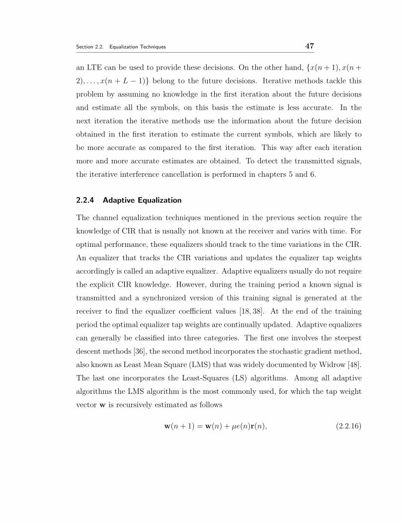
vector w is recursively estimated as follows
w(n+ 1) = w(n) + µe(n)r(n), (2.2.16)
Section 2.3. Cramer Rao Lower Bound 48
where w(n) = [ wo(n) w1(n) · · · wM−1(n) ]T is the tap weight vector estimated
at time index n, µ is the step size, e(n) = d(n)− y(n) is the error between the trans-
mitted and decoded signal at the output of an adaptive equalizer at time n, d(n) is
the training signal and y(n) = wH(n)r(n).
An adaptive equalizer can only track small variations in the channel. If the channel
is fast time varying then the adaptive equalizer can not track the channel variations
that degrade BER performance of the receiver, particularly, when higher constella-
tion points modulation schemes are used [1]. Therefore, in fast time varying channels
conventional block based equalization schemes have to be used that generally require
explicit estimation of the channel parameters.
The efficient estimation of channel parameters is very important to decode the trans-
mitted data accurately. Therefore, before continuing to the estimation techniques to
design an estimator, it is very important to know wether the estimator being designed
is unbiased or biased and if it is unbiased what is its variance about the true value.
An estimator is said to be unbiased iff
E{θ} = θ, a < θ < b (2.2.17)
where a and b represent the end values of an interval that the unknown parameter,
θ, can take on. On the other hand an estimator is said to be biased if
E{θ} = θ − b(θ) (2.2.18)
where b(θ) 6= 0 is the bias in estimation.
2.3 Cramer Rao Lower Bound
To assess the performance of an unbiased estimator to have a lower bound on its
variance is very useful. If an estimator attains this bound for every value of unknown
parameter, θ, to be estimated, then, it is termed the Minimum Variance Unbiased
(MVU) estimator. This lower bound provides the impossibility of determining an

Section 2.3. Cramer Rao Lower Bound 49
estimator, having lower variance than the bound. Among various variance bounds
the Cramer Rao Lower Bound (CRLB) is the easiest to find and most commonly used
in practice. The theory of the CRLB allows the determination of the MVU estimator,
if it exist. If θ is the estimator of θ, then
σ2θ(θ) ≥ CRLBθ(θ) (2.3.1)
where σ2θ(θ) represent the variance of the estimator, θ, that is the best that can be
expected to be done with an unbiased estimator. In order to find the variance of an
unbiased estimator, let us suppose an unbiased estimator, θ of a scalar parameter θ.
Then it can be written as
E{θ} =
∫ ∞
−∞θp(r; θ)dr = θ (2.3.2)
where r represents the N sample receive vector. The regularity condition is
E
{
∂ ln p(r; θ)
∂θ
}
= 0 ∀ θ (2.3.3)
where the E{.} is evaluated with respect to p(r; θ). From (2.3.3) it can be written as
∫ ∞
−∞p(r; θ)
∂ ln p(r; θ)
∂θdr = 0 (2.3.4)
∫ ∞
−∞p(r; θ)
1
p(r; θ)
∂p(r; θ)
∂θdr = 0 (2.3.5)
∂
∂θ
∫ ∞
−∞p(r; θ)dr =
∂1
∂θ= 0 (2.3.6)
Hence, the regularity condition holds true for every value of θ. Differentiation of
(2.3.2) with respect to θ yields
∂
∂θ
∫ ∞
−∞θp(r; θ)dr =
∫ ∞
−∞θ∂p(r; θ)
∂θdr = 1 (2.3.7)
Note that
∂ ln p(r; θ)
∂θ=
1
p(r; θ)
∂p(r; θ)
∂θ(2.3.8)

Section 2.3. Cramer Rao Lower Bound 50
Therefore, using this result (2.3.7) can be written as
∫ ∞
−∞θ∂ ln p(r; θ)
∂θp(r; θ)dr = 1. (2.3.9)
Equation (2.3.4) can be written as
∫ ∞
−∞θ∂ ln p(r; θ)
∂θp(r; θ)dr = 0 (2.3.10)
Subtracting (2.3.10) from (2.3.9) yields
∫ ∞
−∞(θ − θ)
∂ ln p(r; θ)
∂θp(r; θ)dr = 1. (2.3.11)
The Cauchy Schwartz inequality is defined as
(∫
w(r)g(r)h(r)dr
)2
≤∫
w(r)g2(r)dr
∫
w(r)h2(r)dr, provided w(r) ≥ 0 (2.3.12)
and equality holds when g(r) = c h(r), where c is a scalar and not a function of r.
Define,
w(r) = p(r; θ) ,
g(r) = (θ − θ) ,
h(r) =∂ ln p(r; θ)
∂θ.
Squaring (2.3.11) and using the Cauchy Schwartz inequality [30], it can be written as
(∫ ∞
−∞(θ − θ)
∂ ln p(r; θ)
∂θp(r; θ)dr
)2
≤∫ ∞
−∞(θ − θ)2p(r; θ)dr
∫ ∞
−∞
(
∂ ln p(r; θ)
∂θ
)2
p(r; θ)dr
1 ≤ E{
(θ − θ)2}
E
{
(
∂ ln p(r; θ)
∂θ
)2}
(2.3.13)
where E{
(θ − θ)2}
is the definition of the variance of an estimator, θ, therefore
σ2θ(θ) ≥ 1
E
{
(
∂ ln p(r;θ)∂θ
)2} . (2.3.14)

Section 2.3. Cramer Rao Lower Bound 51
In this expression for variance, the expected value of a square term, in the denomi-
nator, is to be found. However, it is more convenient to find the expected value of
a unity power term. Therefore, by differentiating (2.3.4) with respect to θ the unity
power equivalent of this square term can be found as∫ ∞
−∞
∂
∂θp(r; θ)
∂ ln p(r; θ)
∂θdr = 0 (2.3.15)
∫ ∞
−∞
(
∂ ln p(r; θ)
∂θ
∂ ln p(r; θ)
∂θp(r; θ)dr +
∂2 ln p(r; θ)
∂θ2p(r; θ)dr
)
= 0 (2.3.16)
∫ ∞
−∞p(r; θ)
(
∂ ln p(r; θ)
∂θ
)2
dr = −∫ ∞
−∞p(r; θ)
∂2 ln p(r; θ)
∂θ2dr (2.3.17)
E
{
(
∂ ln p(r; θ)
∂θ
)2}
= −E{
∂2 ln p(r; θ)
∂θ2
}
(2.3.18)
Therefore, the variance of the estimator can be written as
σ2θ(θ) ≥ 1
−E{
∂2 ln p(r;θ)∂θ2
} (2.3.19)
Equality is the so called CRLB and the condition for equality is
∂ ln p(r; θ)
∂θ=
1
c(θ − θ) (2.3.20)
where c is a scalar constant whose value may depend on θ. Therefore, this equation
implies that if the log-likelihood function can be written in this form then θ will be
the MVU estimator. By differentiating (2.3.20) again the value of c(θ) can be found
as
∂
∂θ
∂ ln p(r; θ)
∂θ=
∂
∂θ
(
1
c(θ)(θ − θ)
)
(2.3.21)
∂2 ln p(r; θ)
∂θ2= − 1
c(θ)(2.3.22)
c(θ) =1
−E{
∂2 ln p(r;θ)∂θ2
} (2.3.23)
Therefore, if (2.3.20) can be written in general form
∂ ln p(r; θ)
∂θ= I(θ) (g(r) − θ) , (2.3.24)

Section 2.4. Channel Parameter Estimation 52
then g(r) is the MVU estimator. The I(θ) = 1c(θ)
and is termed the Fisher information
[30]. The CRLB derived in this section can easily be extended for vector parameters
and will be used throughout the thesis to assess the performance of the estimators.
2.4 Channel Parameter Estimation
Generally, the parameter estimation in wireless channels includes the estimation of
channel MGs, Frequency Offsets (FOs), phase shift and synchronization pulses. In
this thesis, only the estimation of MGs and FOs is discussed and the remainder of the
parameters are assumed to be known. Channel parameter estimation can be classified
into two broad categories, supervised and non-supervised or blind.
2.4.1 Supervised Parameter Estimation
Supervised or training data assisted (TDA) is a practical parameter estimation tech-
nique in digital mobile communications, it can provide high performance in a fading
environment with large constellations and it has a simple implementation [17,49,50].
Burst digital communication, where the data are transmitted in frames, is used in
various wireless communications systems, such as TDMA, CDMA, and OFDMA. In
the TDA parameter estimation technique a training signal sequence is embedded in-
side the data frames and is more suitable for applications requiring fast and reliable
parameter estimation [21, 51]. In the GSM frame structure, for example, the middle
26 bits in a time slot are dedicated for channel estimation as shown in Figure 2.4.
Nevertheless, this method reduces the effective channel transmission rate as these
extra bits do not contain useful data information bits. TDA parameter estimation
can further be classified into two more categories, parametric, where the sample data
follows a particular probability distribution, and non parametric, where the sample
data does not follow any probability distribution. In the following the parametric and
non-parametric approaches are briefly described.

Section 2.4. Channel Parameter Estimation 53
TS0 TS7 TS6 TS5 TS4 TS3 TS2 TS1
F 3 26 Train 3 F
Frame = 4.615ms
57 Data 57 Data 8.25 G
TS0: Time Slot 0 F: Flag G: Gaurd
Time Slot = 577 us
Figure 2.4. Frame structure of GSM communications.
Maximum Likelihood Estimation: Maximum likelihood estimation (MLE) is the
most popular parametric technique to estimate the parameters. The MLE technique
determines the parameters that maximize the probability (likelihood) of the received
sample data. From a statistical point of view, the MLE technique is considered to
be more robust, versatile, and yields estimators with good statistical properties and
can be applied to most of the data models [30]. Moreover, it provides efficient meth-
ods for quantifying uncertainty through confidence bounds. Although the method-
ology of the MLE is simple, the implementation is computationally expensive. If
r = [ r(0) r(1) · · · r(N − 1) ] is a vector of N received samples with the Proba-
bility Density Function (PDF) p(r ; θ), where θ = [ θ1 θ2 · · · θK ] is a vector of
K unknown constant parameters to be estimated. Then, the likelihood function of
the received samples can be written as
p(r; θ) =N−1∏
i=0
p [r(i); θ1, θ2, ..., θK ] . (2.4.1)
As ln x is a monotonically increasing function of x between 0 and 1, taking the natural
log of (2.4.1) will not affect the maximization, but simplify the problem, therefore
ln[p(r; θ)] =N−1∑
i=0
ln p [r(i); θ1, θ2, ..., θK ] (2.4.2)

Section 2.4. Channel Parameter Estimation 54
Maximizing ln[p(r; θ)], which is much easier to work with than p(r; θ), the MLEs of
the elements of θ are the simultaneous solutions of K equations such that,
∂ ln[p(r; θ)]
∂θi
= 0 ; i = 1, 1, ..., K (2.4.3)
An MLE has three salient properties that are [30].
• It satisfies the condition limN→∞
E{θ} = θ, i.e, it is asymptotically unbiased.
• The distribution of the maximum likelihood estimator is Gaussian.
• It asymptotically attains CRLB. This property of the estimator is termed as
efficiency.
Increase in sample size of a maximum likelihood estimator decreases its variance, this
property is termed as consistency. The draw back of the MLE is its complexity and
it is difficult to apply for the signal models where the noise is not Gaussian.
Example 1: The N received samples in (2.1.1) can be written in vector form as
r = Xh + v (2.4.4)
where
r =[
r(0) r(1) · · · r(N − 1)]T
X =
x(0) x(−1) · · · x(1 − L)
x(1) x(0) · · · x(2 − L)...
. . . . . . · · ·x(N − 1) x(N − 2) · · · x(N − L)
,
h =[
h(0) h(1) · · · h(L− 1)]T
and v =[
v(0) v(1) · · · v(L− 1)]T
.

Section 2.4. Channel Parameter Estimation 55
Here, {x(n)} are transmitted training symbols that are known at the receiver. In
order to estimate h in (2.4.4) the log-likelihood function of r can be written as
ln p(r; h) = ln1
(πσ2)N/2e− (r−Xh)H (r−Xh)
σ2v
=−N2
ln(πσ2) − (r − Xh)H(r − Xh)
σ2v
(2.4.5)
To maximize the likelihood function, differentiating with respect to h (considering
the log-likelihood function is a function of h) yields
∂ ln p(r;h)
∂hH=
1
σ2v
(XHr − XHXh)
=1
σ2v
(XHX){
(XHX)−1XHr − h}
(2.4.6)
Comparing it with (2.3.24) or equating to zero yields the MVU estimator
h = (XHX)−1XHr. (2.4.7)
Example 2: In this example, the joint estimation of h and FO is considered. Here,
it is assumed that the support of the channel is L and each path experiences a DS of
fd. The received sample can be written as
r(n) =L−1∑
l=0
h(l)x(n− l)ej2πfdn + v(n) (2.4.8)
and N received samples in vector form can be written as
r = EoXh + v (2.4.9)
where
Eo =
1 0 0 0
0 ej2πfd 0 0
0 0. . . 0
0 0 0 ej2πfd(N−1)
(2.4.10)

Section 2.4. Channel Parameter Estimation 56
The training signal matrix, X, and MGs vector, h, are defined in the previous ex-
ample. Ignoring the constant terms, as they will not affect the maximization of the
log-likelihood function, for the log-likelihood function to be maximum with respect
to the unknown parameters then
ln p(r;h; fd) = −(r − EoXh)H(r − EoXh) (2.4.11)
or the cost function to minimize is
J(h; fd) = (r − EoXh)H(r − EoXh)
= rHr − rHEoXh − hHXHEHo r + hHXHXh. (2.4.12)
Note that EHo Eo = I. To minimize the cost function with respect to h, by assuming
fd constant, differentiate (2.4.12) with respect to h
∂J(h; fd)
∂h= −XHEH
o r + XHXh, (2.4.13)
equating it to zero yields
h = (XHX)−1XHEHo r. (2.4.14)
In this expression the matrix Eo is unknown and depends on fd, therefore h can
not be estimated. In order to estimate fd, use of (2.4.13) in (2.4.12) yields the cost
function to minimize with respect to fd
J(fd) = rHr − rHEoX(XHX)−1XHEHo r (2.4.15)
The training samples {x(n)} are assumed uncorrelated, therefore XHX ≈ NI. The
minimization of (2.4.15) is equivalent to the maximization of the second term that
can be written as
rHEoXXHEHo r =
γHγ
N
where
γH =[
∑N−1n=0 r(n)ej2πfonx(n) · · · ∑N−1
n=0 r(n)ej2πfonx(n− L+ 1)]
,

Section 2.4. Channel Parameter Estimation 57
and hence
rHEoXXHEHo r =
1
N
N−1∑
n=0
L−1∑
l=0
∣
∣r(n)ej2πfdnx(n− l)∣
∣
2= φ(fd), (2.4.16)
and to estimate DS, fd, the maximum likelihood solution can be written as
fd = arg maxf
φ(f) (2.4.17)
The value of f that maximizes (2.4.17) will be the maximum likelihood estimator
solution for fd and can be used to estimate h in (2.4.14). In order to estimate fd a
grid search method can be used and the accuracy of the estimator depends on the
frequency bin chosen, which is computationally very expensive. However, in practice
a less computationally expensive approach called the Fast Fourier Transform (FFT)
is used.
Least-Squares Estimation: Least-Squares (LSs) estimation is a non-parametric
approach to estimate the parameters and is widely used in practice due to ease of
implementation and optimality in Gaussian noise. Here, no probabilistic assumption
about the data is needed other than the data. Therefore, it can be applied to almost
all types of data model. The disadvantage of the least-squares estimator is that it
does not guarantee the optimality of the estimator. A LSs estimator of an unknown
parameter vector, θ, for a received signal model
r(n) = s(n; θ) + v(n) (2.4.18)
minimizes the Mean Square Error (MSE) between the the deterministic term s(n; θ)
and received data, r(n), as [30]
J(θ) =N−1∑
n=0
[r(n) − s(n; θ)]2 (2.4.19)
Therefore, the estimator
θ = arg minθJ(θ) (2.4.20)

Section 2.5. FO Estimation 58
2.5 FO Estimation
In the above algorithms, to estimate FO, the training based estimation techniques
were considered. However, the FO can be estimated without training data. In the
following, some of the non-TDA estimation techniques are briefly discussed.
2.5.1 Frequency domain transformation
This is the easiest method to established the FOs and is a block based approach to
estimate FOs. Here, the received signal samples are converted into the frequency
domain by taking their discrete Fourier transform (DFT). If the received signal sam-
ples contain more than one FO then the Fourier transform gives peak values at the
FOs provided there is sufficient separation between the offset frequencies. The ampli-
tude of the received samples at different frequencies can be established by using the
discrete Fourier transform relation given by [30,52–54],
F (f) =1
N
N−1∑
n=0
r(n)e−j2πfn (2.5.1)
where F (f) is the complex amplitude of the received signal at frequency f , r(n), is
the received signal sample and N is the number of received samples. The drawback
of using this method is that in the presence of multiple frequency components in
the received signal, it is difficult to find the source corresponding to a particular FO
component. Secondly, this method does not give good performance in the presence
of multipath fading channels.
2.5.2 Sub-space based FO estimation
Sub-space based estimation algorithms such as MUSIC and ESPRIT [55–57] can pro-
vide high resolution frequency estimation at the expense of increased computational
complexity. Sub-spaced based algorithms require eigen or singular value decomposi-
tion of the received sample covariance matrix R to find the signal and noise orthogonal

Section 2.5. FO Estimation 59
sub-spaces i.e., R = VΛVH and V = [VS VN ]. Where Λ is a diagonal matrix of
eigen values of the covariance matrix, while VS and VN contain the basis vectors for
the signal and noise spaces respectively. An inner product of any two vectors from
the orthogonal noise and signal subspaces yields zero and it is this property that is
used to find the FOs of the signal. A draw back in using sub-space based algorithms
is that as the number of frequency components in the received signal increases, the
order of the associated covariance matrix increases. Therefore, to find the singular
value decomposition of a high order covariance matrix extensive computation is re-
quired. The subspace based algorithm MUSIC computes the frequencies of the signal
as the peaks in the MUSIC spectrum estimate given by [56]
SMUSIC(f) =1
sH(f)VNVHNs(f)
(2.5.2)
where s(f) is the frequency scanning vector and is defined by
s(f) =[
1 e−j2πf ... e−j2πfM
]T
(2.5.3)
and M is the order of the covariance matrix.
2.5.3 Un-supervised Parameter Estimation
In an un-supervised or blind parameter estimation technique, a training signal is
theoretically assumed not to be needed. Hence, it has the potential to increase the
overall capacity of the communication system. Here, the cost function based on some
already known quantity, such as the modulus or energy of the transmitted signal
is optimized to find some parameters. Blind algorithms generally take substantially
more time to estimate the parameters and assume the channel is not changing rapidly.
Therefore, they are not good for burst communication, where small numbers of bits
are available. Although they have much potential where the channel is very slowly
changing, as in fixed telephone networks. A number of blind parameter estimators is
given in [58–60] and the references therein.

Section 2.6. Summary 60
2.6 Summary
In this chapter, a foundation was provided to proceed to mitigate the effects of time-
varying multipath channels. First of all the fundamental question: what are the causes
and how the effects of multipath channels are mitigated was answered. To mitigate
the effects of a multipath channel the technology of equalization was introduced and
several linear, nonlinear and adaptive equalization techniques were discussed briefly.
In fast fading channels, it was highlighted that it is difficult for an adaptive equal-
izer to track the channel variations, thereby degrading the BER performance of the
system. Therefore, in the fast fading environment conventional equalizers are used
that require the accurate knowledge of the channel. The performance of these equal-
izers depends on the variance of the channel parameter estimators, therefore, a bench
mark on the variance of an unbiased estimator, the CRLB was derived to assess the
performances of various unbiased estimators. Then some optimal and non-optimal
parameter estimation techniques were discussed briefly.
Chapter 3
PARAMETER ESTIMATION AND
EQUALIZATION IN SISO WITH
FREQUENCY OFFSETS
Wireless transmission is impaired by signal fading, interference and additive noise.
Moreover, the presence of FO introduces the time-variations into the multipath chan-
nel that degrade the BER performance of a communication system, particularly one
based on the assumption that the channel is time-invariant. There are two main
causes for FOs; poor synchronization between the transmitter and the receiver car-
rier frequencies and the motion-induced DS due to the relative motion between the
mobile station and the local scatterers [61]. The reason for poor synchronization could
be due to an error in the crystal oscillator frequency or due to temperature variations.
If the FO is due to temperature variations, then it will be slowly time-varying as the
temperature changes are not very abrupt and may take a longer time to cause the
frequency of the oscillators to drift. The FO due to DS may be random and fast
time-varying. Therefore, the overall FO, fo, can be written as [62].
fo = fd + fse (3.0.1)
where fd is the DS and fse is the frequency synchronization error between the trans-
mitter and the receiver local oscillator frequencies. The estimation of FO and its
exploitation in equalization is crucial to enable accurate decoding of the transmitted
61
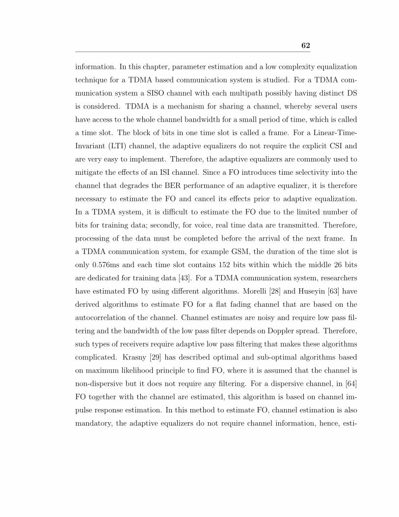
62
information. In this chapter, parameter estimation and a low complexity equalization
technique for a TDMA based communication system is studied. For a TDMA com-
munication system a SISO channel with each multipath possibly having distinct DS
is considered. TDMA is a mechanism for sharing a channel, whereby several users
have access to the whole channel bandwidth for a small period of time, which is called
a time slot. The block of bits in one time slot is called a frame. For a Linear-Time-
Invariant (LTI) channel, the adaptive equalizers do not require the explicit CSI and
are very easy to implement. Therefore, the adaptive equalizers are commonly used to
mitigate the effects of an ISI channel. Since a FO introduces time selectivity into the
channel that degrades the BER performance of an adaptive equalizer, it is therefore
necessary to estimate the FO and cancel its effects prior to adaptive equalization.
In a TDMA system, it is difficult to estimate the FO due to the limited number of
bits for training data; secondly, for voice, real time data are transmitted. Therefore,
processing of the data must be completed before the arrival of the next frame. In
a TDMA communication system, for example GSM, the duration of the time slot is
only 0.576ms and each time slot contains 152 bits within which the middle 26 bits
are dedicated for training data [43]. For a TDMA communication system, researchers
have estimated FO by using different algorithms. Morelli [28] and Huseyin [63] have
derived algorithms to estimate FO for a flat fading channel that are based on the
autocorrelation of the channel. Channel estimates are noisy and require low pass fil-
tering and the bandwidth of the low pass filter depends on Doppler spread. Therefore,
such types of receivers require adaptive low pass filtering that makes these algorithms
complicated. Krasny [29] has described optimal and sub-optimal algorithms based
on maximum likelihood principle to find FO, where it is assumed that the channel is
non-dispersive but it does not require any filtering. For a dispersive channel, in [64]
FO together with the channel are estimated, this algorithm is based on channel im-
pulse response estimation. In this method to estimate FO, channel estimation is also
mandatory, the adaptive equalizers do not require channel information, hence, esti-

Section 3.1. Problem statement 63
mation of the channel and FO increases the complexity of the receiver. Harish [20]
proposed a maximum state accumulation technique of FO estimation that does not
require an explicit estimation of the channel. All the above algorithms, assume that
the FO is identical from each multipath.
In contrast to previous work, in this chapter, equalization for a single transmit and
receive antenna, under a general framework that allows distinct FOs from each multi-
path, is addressed. Such a scenario may arise when either the receiver or the transmit-
ter moves at high speed, thereby, resulting in distinct DSs for the multipaths due to
different angle of arrival. In this scenario, most of the above FO estimation algorithms
cannot be applied. Therefore, for this scenario, exploiting the correlation property
of the transmitted training symbols, an Approximative Maximum Likelihood (AML)
estimator is proposed. Here, unlike the identical DS problem, the distinct DSs can
not be compensated for prior to equalization and have to be accounted for in equalizer
design. Now, it is imperative to use the conventional block-based equalizer design.
In multipath with distinct FO scenario, it is further shown that the conventional
MMSE equalizer is computationally cumbersome as the effective CCM changes de-
terministically between symbols. However, by exploiting the structural property of
these changes, a computationally efficient recursive algorithm for the equalizer design
is proposed.
3.1 Problem statement
Consider a communication system employing a single transmit and receive antenna,
and assume that the signal has propagated through L different paths, each having
different FOs and complex MGs. If the sampling rate is equal to the symbol trans-
mission rate then the received baseband signal can be written as
r(n) = r(n) + v(n) =L−1∑
l=0
hlx(n− l)ej2πfln + v(n), (3.1.1)
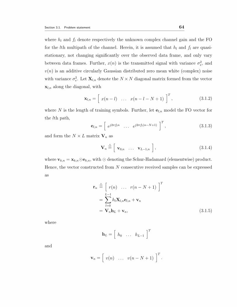
Section 3.1. Problem statement 64
where hl and fl denote respectively the unknown complex channel gain and the FO
for the lth multipath of the channel. Herein, it is assumed that hl and fl are quasi-
stationary, not changing significantly over the observed data frame, and only vary
between data frames. Further, x(n) is the transmitted signal with variance σ2x, and
v(n) is an additive circularly Gaussian distributed zero mean white (complex) noise
with variance σ2v . Let Xl,n denote the N ×N diagonal matrix formed from the vector
xl,n along the diagonal, with
xl,n =[
x(n− l) . . . x(n− l −N + 1)]T
, (3.1.2)
where N is the length of training symbols. Further, let el,n model the FO vector for
the lth path,
el,n =[
ej2πfln . . . ej2πfl(n−N+1)
]T
, (3.1.3)
and form the N × L matrix Vn as
Vn△=[
v0,n . . . vL−1,n
]
, (3.1.4)
where vk,n = xk,n⊙ek,n, with ⊙ denoting the Schur-Hadamard (elementwise) product.
Hence, the vector constructed from N consecutive received samples can be expressed
as
rn△=[
r(n) . . . r(n−N + 1)]T
=L−1∑
l=0
hlXl,nel,n + vn
= VnhL + vn, (3.1.5)
where
hL =[
h0 . . . hL−1
]T
and
vn =[
v(n) . . . v(n−N + 1)]T
.

Section 3.2. Estimation of multipath gains and frequency offsets 65
Here, the problem of interest is given rn and the training symbols {x(n)}, estimate
the unknown parameter vector
θ =[
h0 . . . hL−1 f0 . . . fL−1
]T
△=[
hTL fT
L
]T
(3.1.6)
where fL = [f0 f1 . . . fL−1]T . Here, no explicit knowledge on the channel length is
required, other than the knowledge on its upper bound. For an over modelled system,
the estimates of the additional channel coefficients would be close to zero and in this
way the channel length can potentially be determined. In the next section, to estimate
the unknown MGs and FOs a computationally efficient approach is presented.
3.2 Estimation of multipath gains and frequency offsets
In this section, an approximative maximum likelihood (AML) estimator of the com-
plex MGs and the FOs is outlined. Consider that the received signal, as expressed in
(3.1.5), is only a function of the complex MGs and FOs. The likelihood function, of
the received sample vector, to be maximized can be written as
p(rn|θ) =1
(πσ2v)
Ne
−(rn−VnhL)H(rn−VnhL)σ2
v (3.2.1)
where the probability of an event occurring can be between 0 and 1, and lnx is a
monotonically increasing function for x ǫ {0, 1}. Therefore, the log-likelihood function
will not have any effect on the maximization problem, the log-likelihood function can
be expressed as (ignoring the constant terms)
ln p(rn|θ) = − 1
σ2v
(rn − VnhL)H (rn − VnhL) . (3.2.2)
Maximization of (3.2.2) with respect to hL yields [30]
hL =(
VHn Vn
)−1VH
n rn△= V†
nrn, (3.2.3)

Section 3.2. Estimation of multipath gains and frequency offsets 66
where V†n denotes the Moore-Penrose pseudo-inverse. The FOs are estimated by
minimizing the cost function, J(fL), obtained by substituting equation (3.2.3) into
(3.2.2),
J(fL) = rHn rn − rH
n ΠVnrn, (3.2.4)
where ΠVn= VnV
†n is the projection onto the range space of Vn. By choosing the
training sequence, x(n), such that E{
x∗(n− l)x(n− p)}
= δp−l, where δk denotes
the Kronecker delta function and (·)∗ the conjugate, the n-dimensional minimiza-
tion problem in (3.2.4) may be decoupled into n one-dimensional problems, which
significantly reduces the complexity of the minimization. Note that VHn Vn will be
dominated by the large diagonal terms, with almost negligible contribution from the
off-diagonal terms, if x(n) is chosen as a pseudo-random sequence (as in the case of
a training signal). Thus, VHn Vn ≈ ∑N−1
n=0 |x(n)|2 I△= κI, where κ is constant over
the frame considered, enabling the minimization of (3.2.4) to be approximated as the
maximum of
J ′(fL) = rHVnVHn rn
=L−1∑
p=0
∣
∣
∣
∣
∣
N−1∑
n=0
r∗(n)x(n− p)ej2πfpn
∣
∣
∣
∣
∣
2
(3.2.5)
This is a difficult joint multi-dimensional optimization problem. Therefore, the FO of
an arbitrary individual path s between a transmit and a receive antenna is considered,
for which the contribution to (3.2.5) is
ψs(n) = r∗(n)x(n− s)ej2πfsn
= Qs + c1(n) + c2(n) (3.2.6)

Section 3.3. Numerical Example for Variance of Estimators 67
where
Qs = h∗s |x(n− s)|2 ,
c1(n) = v∗(n)x(n− s)ej2πfsn,
c2(n) =L−1∑
p=0
p 6=s
h∗p(p)x∗(n− p)x(n− s)ej∆2πfpn
∆fp = fs − fp
Moreover, as E{x(n− u)x(n− v)} = 0 for u 6= v,
∣
∣
∣
∣
∣
N−1∑
n=0
ψs(n)
∣
∣
∣
∣
∣
2
≈ N2|hs|2|x(n− s)|4 +N
L−1∑
p=0
p 6=s
|hp|2|x(n− p)|2|x(n− s)|2
= N2ρs +Nρi
≈ N2ρs (For large N) (3.2.7)
Therefore, provided that the ratio between the signal component for which the pa-
rameters are to be estimated, ρs = |hs|2|x(n − s)|4, to the interfering components
ρi =∑L−1
p=0p 6=s
|hp|2|x(n−p)|2|x(n−s)|2, is greater than 1/N , the joint multi-dimensional
maximization problem in (3.2.5) can be reduced over all possible frequencies to the
maximization of the following for each individual frequency
fs = arg maxf
∣
∣
∣
∣
∣
N−1∑
n=0
r∗(n)x(n− s)ej2πfn
∣
∣
∣
∣
∣
2
(3.2.8)
which can be efficiently evaluated using the fast Fourier transform (FFT). Once the
FOs are estimated, the MGs, hk , can be estimated using (3.2.3).
3.3 Numerical Example for Variance of Estimators
In order to assess the performance of the proposed AML estimator, a two-tap chan-
nel with FOs f0 = 0.003 and f1 = 0.005 is considered. This is reasonable as the

Section 3.3. Numerical Example for Variance of Estimators 68
maximum DS for a vehicular speed of 250 km/h (RA250 channels as defined in GSM
standards) at a carrier frequency of 1800 MHz is 416Hz, which corresponds to 0.005
when normalized to the symbol rate of 100 kHz as in GSM [43]. The number of
training samples to estimate MGs and FOs is N = 100. Training samples are as-
sumed binary alphabets. Figures 3.1 and 3.2 show that the mean-square estimation
error as obtained from 104 Monte-Carlo simulations attains the Cramer-Rao lower
bound (CRLB), derived in the Appendix 3A. The complex channel gains h0 and h1
have been assumed to be constant throughout a burst, but may change between the
frames.
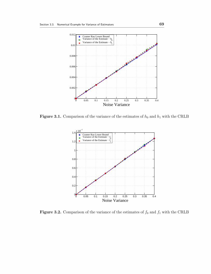
Section 3.3. Numerical Example for Variance of Estimators 69
0 0.05 0.1 0.15 0.2 0.25 0.3 0.35 0.40
0.002
0.004
0.006
0.008
0.01
0.012
Noise Variance
Cramer Rao Lower BoundVariance of the Estimate − h
0Variance of the Estimate − h
1
Figure 3.1. Comparison of the variance of the estimates of h0 and h1 with the CRLB
0 0.05 0.1 0.15 0.2 0.25 0.3 0.35 0.40
0.2
0.4
0.6
0.8
1
1.2
1.4x 10
−7
Noise Variance
Cramer Rao Lower BoundVariance of the Estimate − f
0Variance of the Estimate − f
1
Figure 3.2. Comparison of the variance of the estimates of f0 and f1 with the CRLB

Section 3.4. MMSE equalizer design 70
3.4 MMSE equalizer design
As discussed earlier, identical FOs from each multipath can be compensated for easily
before equalization, distinct FOs are difficult to compensate for easily. Distinct FOs
produce time selectivity in the channel that not only degrades the BER performance
but increases the computational complexity of the classical equalizers.
3.4.1 Equalizer for channels without FOs
In this section, initially the MMSE equalizer for the communication channel not
affected by multiple FOs is considered. Consider the received baseband signal in
(6.2.1), for the case when fp = 0. For an equalizer of length M , the received signal
vector can then be written as
rn = Hxn + ηn, (3.4.1)
where
rn =[
r(n) . . . r(n−M + 1)]T
,
xn =[
x(n) . . . x(n−M − L+ 2)]T
,
ηn =[
v(n) . . . v(n−M + 1)]T
and H is the M × (L+M − 1) CCM,
H =
hTL 0 . . . 0
0 hTL 0
...... 0
. . . 0
0 . . . 0 hTL
(3.4.2)
The MMSE equalizer, wo, [30, 65] for the estimation of x(n) is found by minimizing
the cost function
J(wo) = |x(n) − wHo rn|2 (3.4.3)
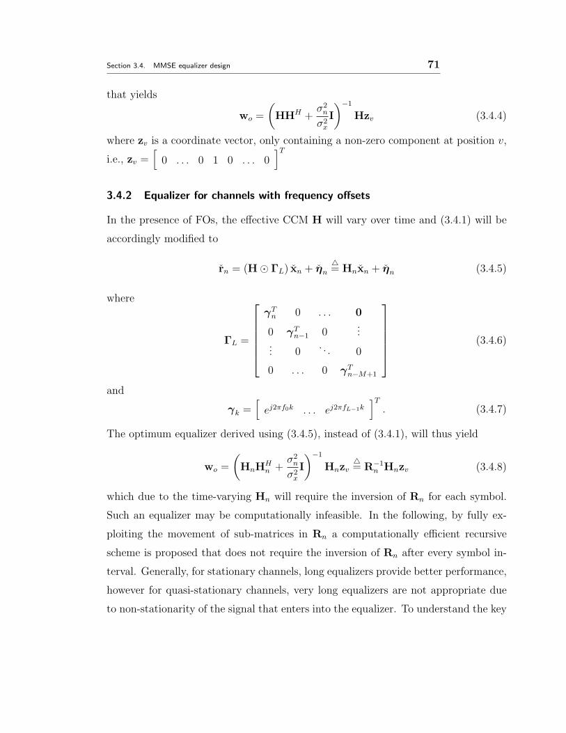
Section 3.4. MMSE equalizer design 71
that yields
wo =
(
HHH +σ2
n
σ2x
I
)−1
Hzv (3.4.4)
where zv is a coordinate vector, only containing a non-zero component at position v,
i.e., zv =[
0 . . . 0 1 0 . . . 0]T
3.4.2 Equalizer for channels with frequency offsets
In the presence of FOs, the effective CCM H will vary over time and (3.4.1) will be
accordingly modified to
rn = (H ⊙ ΓL) xn + ηn
△= Hnxn + ηn (3.4.5)
where
ΓL =
γTn 0 . . . 0
0 γTn−1 0
...... 0
. . . 0
0 . . . 0 γTn−M+1
(3.4.6)
and
γk =[
ej2πf0k . . . ej2πfL−1k
]T
. (3.4.7)
The optimum equalizer derived using (3.4.5), instead of (3.4.1), will thus yield
wo =
(
HnHHn +
σ2n
σ2x
I
)−1
Hnzv△= R−1
n Hnzv (3.4.8)
which due to the time-varying Hn will require the inversion of Rn for each symbol.
Such an equalizer may be computationally infeasible. In the following, by fully ex-
ploiting the movement of sub-matrices in Rn a computationally efficient recursive
scheme is proposed that does not require the inversion of Rn after every symbol in-
terval. Generally, for stationary channels, long equalizers provide better performance,
however for quasi-stationary channels, very long equalizers are not appropriate due
to non-stationarity of the signal that enters into the equalizer. To understand the key

Section 3.4. MMSE equalizer design 72
ideas behind the proposed algorithm, for simplicity, consider a simple example with
only three channel taps and a length three equalizer. Thus,
Rn =
α11 α12 α13
α∗12 α22 α23
α∗13 α∗
23 α33
△=
An
α13
α23
α∗13 α∗
23α33
(3.4.9)
Note that, due to the structure of Rn,
Rn+1 =
β11 β12 β13
β∗12 α11 α12
β∗13 α∗
12 α22
=
β11 β12 β13
β∗12
β∗13
An
(3.4.10)
the Hermitian matrix An will appear in both Rn and Rn+1. This structural property
will hold for any number of channel coefficients and equalizer taps. For the general
case, Rn is written as
Rn =
An cn
cHn bn
(3.4.11)
where An ∈ C(M−1)×(M−1), cn ∈ C(M−1)×1 and bn ∈ R. Provided that the relevant
inverses exist, the inverse of a general block matrix can be expressed as (3.4.12) or
(3.4.13) (see, e.g., [53, 66]).
A C
D B
−1
=
I
0
A−1[
I 0
]
+
−A−1C
I
(
B − DA−1C)−1[
−DA−1 I
]
(3.4.12)
=
0
I
B−1[
0 I
]
+
I
−B−1D
(
A − CB−1D)−1[
I −CB−1]
(3.4.13)
Thus, given A−1n , one can easily obtain R−1
n and R−1n+1, avoiding the matrix inversion.
As An does not appear in Rn+2, it can not be used to find R−1n+2, and the scheme so
far thus only allows for a pairwise computational saving, still requiring the inversion
Section 3.5. Simulations 73
of An+1 to compute R−1n+2 efficiently. However, further exploiting the structure of Rn,
one may compute A−1n+1 efficiently from R−1
n+1 using the following lemma.
Lemma 1: Let
H11 H12
H21 H22
=
A11 A12
A21 A22
−1
(3.4.14)
where dim {Hkl} = dim {Akl}. Then, provided that the relevant inverses exist, the
inverse of matrix A11 can be written as the Schur complement of H22, i.e.,
A−111 = H11 − H12H
−122 H21 (3.4.15)
The proof is given in Appendix 3B. At time n, let us find the inverse of submatrix
An, and use it respectively to find the inverses of Rn and Rn+1 using (3.4.12) and
(3.4.13). Since the inverse of Rn+1 is known, the inverse of the new top left hand corner
submatrix, An+1, can be found by using Lemma 1. Once found the inverse of An+1
can be used to compute the inverse of Rn+2 using (3.4.13). This is called a forward
and backward recursion method to estimate the transmitted symbols. Therefore, the
explicit inverse of the matrix An is needed only once and thereafter, the equalizer is
updated for every symbol with the forward and backward recursions method using
(3.4.13) and Lemma 1. Note that for this problem, H22 is a scalar.
3.5 Simulations
In order to demonstrate the benefits of employing FOs in equalization, a two path
wireless communication channel and an equalizer of length 10 is considered. It is
assumed that the channel is quasi-stationary. The FOs have been initially set to 0.003
and 0.005, and at every burst n they have been changed according to the random walk
model, fl(n) = fl(n− 1) + 0.0001u(n), where u(n) is a zero mean real Gaussian noise
with unity variance. The complex channel gains h0 and h1 have been assumed to be
constant throughout a burst, but change between the frames. The training signal is
assumed to have a binary alphabet while the data symbols in the burst have been
Section 3.5. Simulations 74
drawn from an 8-PSK constellation. Here, three scenarios are considered. In the first
scenario, the FOs associated with the first and the second paths are set f0=0.003 and
f1=0.005, and a recursive equalizer is designed as explained previously. In the second
scenario, to equalize the channel effects a decision directed scheme is adopted, where
the least mean square (LMS) algorithm is used to control the equalizer parameters.
Here, the LMS equalizer is initialized with the correct MMSE solution, found at the
end of the training interval. In the last scenario an equalizer is designed ignoring the
effect of FOs. The results depicted in Figure 3.3 show the superior performance of our
proposed scheme over the decision directed scheme and an equalizer not considering
the effect of FOs. In all the simulation, a training signal of length 142 is considered
for the estimation of the channel parameters including the FOs. The proposed scheme
can also be employed in a GSM system. Here, the number of pilot symbols available
in a burst is only 26. With this training length the channel can be estimated very
efficiently, but to estimate FO this length is insufficient. However, the performance of
the FO estimator can be enhanced, by concatenating the pilot symbols from a number
of recent past bursts. To illustrate this, GSM burst transmission through a two path
time varying channel identical to that used in the previous simulation is simulated.
A normal burst in GSM consists of 116 encrypted data symbols and 26 pilot symbols
in the middle [43]. At every burst the MGs h0 and h1 were estimated using the
pilot symbols, but the FOs have been estimated using 142 symbols from the previous
burst obtained with the retrieved data symbols together with the pilot symbols, in
this way to estimate FOs 5 previous successive bursts are used. To avoid occasional
FO estimation error, the FO estimates are filtered through a moving median filter of
length five. The BER performance of our proposed scheme for a BPSK modulation
scheme is identical to the performance of a GSM communication channel without
FOs as shown in Figure 3.4.

Section 3.5. Simulations 75
0 2 4 6 8 10 12 14 16 18 2010
−2
10−1
100
8PSK constellations
Eb/No
BE
R
MMSE Equalizer when frequency offsets are accountedDecesion Directed EqualizerMMSE Equalizer when frequency offsets are not accounted
Figure 3.3. Bit error rate performance for MMSE equalizers with and without FO
estimation, and a decision directed adaptive equalizer
0 1 2 3 4 5 6 7 8 9 1010
−3
10−2
10−1
100
Eb/No
BE
R
BPSK constellations
The proposed equalizerThe conventional equalizer for zero frequency offsets
Figure 3.4. Bit error rate performance of MMSE equalizers for a GSM system

Section 3.6. Summary 76
3.6 Summary
In this chapter, the estimation and equalization of a frequency selective channel with
distinct FOs was considered. This problem could arise, when the receiver or trans-
mitter moves with very high speed with different paths experiencing distinct DSs, due
to different angle of arrival. By exploiting the correlation property of the transmitted
pilot signal, an AML estimator was provided and it was shown that the estimation
error variance attained the CRLB. Since, in multipath and multiple FO scenario, the
effective CCM varies deterministically between symbols, a recursive scheme to design
the optimum equalizer for every symbol is provided. The simulation results demon-
strated the superior performance of the proposed scheme over an equalization scheme
that did not consider the effects of multiple FOs.
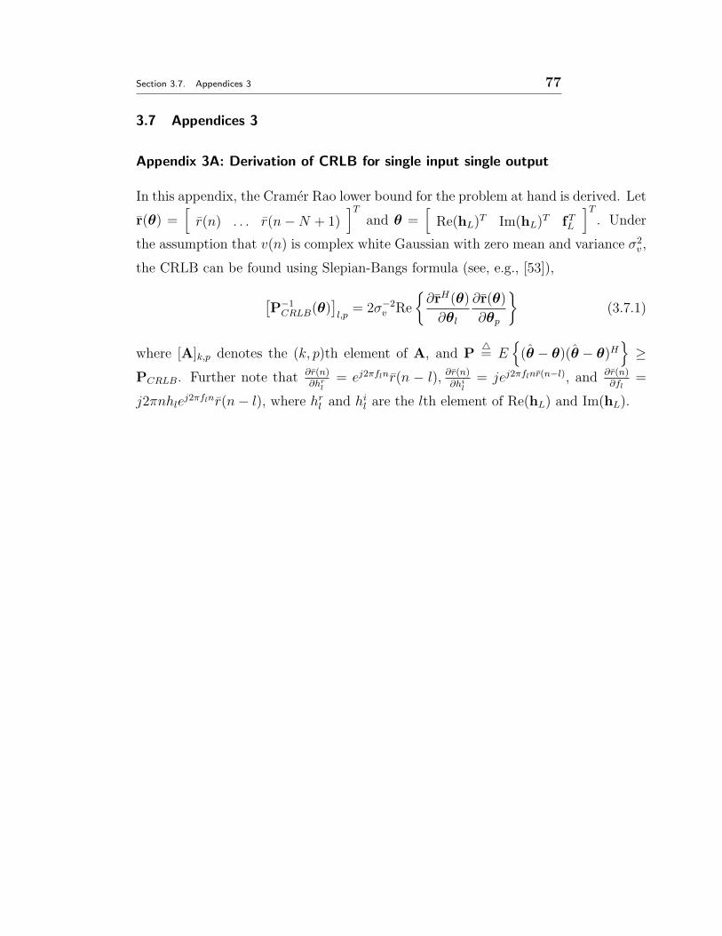
Section 3.7. Appendices 3 77
3.7 Appendices 3
Appendix 3A: Derivation of CRLB for single input single output
In this appendix, the Cramer Rao lower bound for the problem at hand is derived. Let
r(θ) =[
r(n) . . . r(n−N + 1)]T
and θ =[
Re(hL)T Im(hL)T fTL
]T
. Under
the assumption that v(n) is complex white Gaussian with zero mean and variance σ2v ,
the CRLB can be found using Slepian-Bangs formula (see, e.g., [53]),
[
P−1CRLB(θ)
]
l,p= 2σ−2
v Re
{
∂rH(θ)
∂θl
∂r(θ)
∂θp
}
(3.7.1)
where [A]k,p denotes the (k, p)th element of A, and P△= E
{
(θ − θ)(θ − θ)H}
≥PCRLB. Further note that ∂r(n)
∂hrl
= ej2πflnr(n − l), ∂r(n)
∂hil
= jej2πflnr(n−l), and ∂r(n)∂fl
=
j2πnhlej2πflnr(n− l), where hr
l and hil are the lth element of Re(hL) and Im(hL).

Section 3.7. Appendices 3 78
Appendix 3B: Proof of Lemma 1
Using the block matrix inversion lemma, as expressed in (3.4.12) and (3.4.13), (3.4.14)
can be written as (see, e.g., [53, 66])
H11 = A−111 + A−1
11 A12∆−1A A21A
−111 (3.7.2)
H12 = −A−111 A12∆
−1A (3.7.3)
H21 = −∆−1A A21A
−111 (3.7.4)
H22 = ∆−1A (3.7.5)
where ∆A = A22 −A21A−111 A12 is the Schur complement of A11. Substituting (3.7.5)
into (3.7.4), and (3.7.3) into (3.7.2), yields
H21 = −H22A21A−111 (3.7.6)
H11 = A−111 − H12A21A
−111 (3.7.7)
Substituting (3.7.6) into (3.7.7) yields
H11 = A−111 + H12H
−122 H21 (3.7.8)
and hence (3.4.15), which concludes the proof.

Chapter 4
PARAMETER ESTIMATION AND
EQUALIZATION IN MIMO WITH
FREQUENCY OFFSETS
To increase the channel capacity and reliability of a communication system, the in-
formation data can be transmitted and received by using a number of transmit and
receive antennas [67]. This configuration of the communication system is called a
MIMO system. Recent research in communication theory [68] has demonstrated
that large gains in capacity and reliability of communications over wireless channels
can potentially be achieved by exploiting spatial diversity through MIMO anten-
nas [69–71]. Spatial diversity can be used to either increase the capacity or enhance
coverage in a wireless communication system. In the first case, multiple antennas are
used at the transmitter and the receiver to form multiple spatial channels to transmit
multiple data streams through various spatial modes, which is termed data multiplex-
ing [31, 32, 72]. In the second case, multiple antennas are used to transmit multiple
copies of the same data so that a better BER performance can be obtained at very
low SNR [73, 74]. This is exploited to increase the coverage in a wireless commu-
nication system. Therefore, multiple antennas at both the transmitter and receiver
are very likely to play a key role in future high data rate wireless communication
systems. Often, MIMO transmission schemes proposed in the literature are based
79
Section 4.1. Problem Statement 80
on somewhat idealized assumptions. Such as most MIMO transmission schemes are
designed for frequency-flat channels [33, 73]. However, if there are multipath signals
with large propagation delays, then the assumption of frequency-flat channel might
not be valid, depending on the symbol duration.
Besson et al. [33] discussed the estimation of FOs in MIMO flat fading channels with
distinct FOs between each transmitter and receiver. This chapter extend this work
for MIMO frequency selective channels that allows distinct FOs for each multipath
between each transmit and receive antenna. As discussed in chapter 1, the perfor-
mance of such multiple antenna based systems may seriously degrade in the presence
of FOs. Therefore, it is of importance to determine these FOs and to take them into
account for in the equalizer design. In this scenario, to estimate the FOs and MGs, an
AML estimator is proposed that exploits the correlation property of the transmitted
training sequence. In order to assess the performance of the proposed estimator the
corresponding CRLB is determined, and used as a benchmark for the performance
of the proposed estimator. Furthermore, multiple FOs introduce deterministic time
variations in the channel, which are exploited to design a low complexity MIMO
recursive MMSE equalizer to account for symbol-by-symbol variations in the CCM.
4.1 Problem Statement
Consider a MIMO communication system with nT transmit and nR receive antennas,
where the signal between any two transmit and receive antennas has propagated
through a total of L different paths, with each path possibly having different FO. If
the sampling rate at the receive antenna k is equal to the symbol transmission rate
then the received baseband signal can be written as
rk(m) = uk(m) + vk(m), (4.1.1)

Section 4.1. Problem Statement 81
where
uk(m) =
nT∑
l=1
L−1∑
p=0
hkl(p)ejωklpmxl(m− p), (4.1.2)
for m = n, . . . , n−N + 1, k = 1, . . . , nR, where N is the number of symbols received,
hkl(p) and ωklp are respectively the MGs and FOs between the receive antenna k and
the transmit antenna l, for the multipath p; these are assumed to be quasi-stationary,
i.e., they do not change significantly over an observed data frame, but may change be-
tween the frames. Here, {xl(m)} is the training signal sequence, transmitted from the
lth transmit antenna and vk(m) is assumed an additive zero mean circularly Gaussian
distributed, spatially and temporally uncorrelated, white noise with variance σ2v . Let
Xlp = diag{
xlp
}
, where diag{q} denotes a diagonal matrix with the vector q along
the diagonal, and
xlp =[
xl(n− p) · · · xl(n− p−N + 1)]T
(4.1.3)
ekl(p) =[
ejωklpn · · · ejωklp(n−N+1)
]T
(4.1.4)
hkl =[
hkl(0) · · · hkl(L− 1)]T
(4.1.5)
where the vector ekl(p) contains the FO between the receive antenna k and the trans-
mit antenna l, for the multipath p and hkl is the vector of MGs between the receive
antenna k and the transmit antenna l. Furthermore, suppose that
Vkl =[
Xl0ekl(0) · · · Xl(L−1)ekl(L− 1)]
, N × L (4.1.6)
hk =[
hTk1 hT
k2 · · · hTknT
]T
, nTL× 1 (4.1.7)
Vk =[
Vk1 Vk2 · · · VknT
]
. N × nTL (4.1.8)
Using these identities, the N received samples in (4.1.1) can be written in vector form
as
rk =[
rk(n) · · · rk(n−N + 1)]T
= Vkhk + vk. (4.1.9)
Section 4.2. Estimation of Multipath Gains and Frequency Offsets 82
To estimate the various MGs and the FOs, suppose
ωkl =[
ωkl0 ωkl1 · · · ωkl(L−1)
]T
(4.1.10)
and ωk =[
ωTk1 ωT
k2 · · · ωTknT
]T
nTL× 1 (4.1.11)
then, the unknown parameter vector, θk, corresponding to receive antenna k, to be
estimated can be written as θk =[
hTk ωT
k
]T
. In the next section, the problem of
estimating θk is considered.
4.2 Estimation of Multipath Gains and Frequency Offsets
In this section, an approximate maximum likelihood (AML) estimator is outlined,
which fully exploits the structure of the transmitted training sequence. Since the
noise, vk(n), at the receive antenna is spatially uncorrelated, the parameters asso-
ciated with each receiver can be estimated independently from the received signal.
Considering (4.1.9), the likelihood function of rk can be written as [30]
p(rk| θk) =1
(πσ2v)
Ne− (rk−Vkhk)H(rk−Vkhk)
σ2v , (4.2.1)
Taking the natural logarithm and ignoring the constant terms, as they will not affect
the maximization of the likelihood function, (4.2.1) can be written as
ln p(rk| θk) = − 1
σ2vk
(rk − Vkhk)H (rk − Vkhk) . (4.2.2)
In order to estimate parameter vector, θk, maximization of (4.2.1) is equivalent to the
minimization of (4.2.2) (as the minus sign is omitted in the log-likelihood function)
with respect to hk and yields
hk = (VHk Vk)
−1VHk rk, (4.2.3)
then, inserting hk into (4.2.2) yields the cost function to minimize with respect to the
FOs
J(ωklp) = rHk rk − rH
k Vk(VHk Vk)
−1VHk rk. (4.2.4)

Section 4.2. Estimation of Multipath Gains and Frequency Offsets 83
Note that minimizing (4.2.4) requires an nTL-dimensional minimization. However,
choosing the training sequence {xl(n)} such that
E {x∗l (n− u)xd(n− v)} = δu−vδl−d, (4.2.5)
this minimization can be decoupled into nTL one-dimensional minimizations. Con-
sidering (??), note that VHk Vk will be dominated by the large diagonal terms, with al-
most negligible contribution from the off-diagonal terms. Thus, VHk Vk ≈∑N−1
n=0 |xl(n)|2 I△=
κI, where κ is constant over the frame considered, enabling us to approximate the
minimum of (4.2.4) as the maximum of
J ′(ωklp) = rHk VkV
Hk rk
=
nT∑
l=1
L−1∑
p=0
∣
∣
∣
∣
∣
N−1∑
n=0
r∗k(n)xl(n− p)ejωklpn
∣
∣
∣
∣
∣
2
. (4.2.6)
Maximizing J ′(ωklp) is equivalent to maximizing all individual terms of the above
outer sum. Consider a given path s from the transmit antenna q to the receive
antenna k, the contribution of this path to the cost function, J ′(ωklp), can be written
as
ψkqs(n) = r∗k(n)xq(n− s)ejωkqsn
and using (4.1.1) ψkqs(n) = h∗kq(s) |xq(n− s)|2 + c1(n) + c2(n), (4.2.7)
where
c1(n) = v∗k(n)xq(n− s)ejωkqsn
c2(n) =
nT∑
l=1
L−1∑
p=0
p 6=s| l=q
h∗kl(p)x∗l (n− p)xq(n− s)ej∆ωklpn,
and ∆ωklp = ωkqs−ωklp. The first term in ψkqs(n) corresponds to the signal power for
the path s, and as E{x∗l (n−u)xd(n−v)} = 0 for u 6= v, or l 6= d, it will be significantly
larger than the contribution from the interference term, c2(n), constructed from all

Section 4.3. Numerical Example for the Variance of the Estimators 84
paths except p 6= s when transmit antenna l = q. Thus, each of the terms in the
outer sum of (4.2.6) will be maximized for ω = ωkqs, suggesting the AML estimator
for ωkqs, for q = 1, . . . , nT , and s = 0, . . . , L− 1, as
φkqs(ω) =
∣
∣
∣
∣
∣
N−1∑
n=0
r∗k(n)xq(n− s)ejωn
∣
∣
∣
∣
∣
2
(4.2.8)
ωkqs = arg maxω
φkqs(ω), (4.2.9)
which can be efficiently evaluated using the FFT. Once the FOs are estimated, the
MGs, hk , can be estimated by inserting the estimated values of the FOs in (4.2.3).
It can be noted that the AML for FOs does not provide the block based solution but
for MGs, the AML solution is block based.
4.3 Numerical Example for the Variance of the Estimators
To illustrate the theoretical findings a numerical example is provided. Consider a
case with maximum vehicular speed of 250km/h, at a carrier frequency of 1800MHz
(RA250 channels as defined in GSM standard [43]), this corresponds to the maxi-
mum DS of 0.005 when normalized to the symbol rate of 100kbits/sec, which will be
different for different angles of arrivals. For higher carrier frequency or speed, the
normalized frequency will further increase. In order to see the performance of the
proposed estimator, a case using two transmit and two receive antennas is simulated.
Here, it is considered that there are two paths between each transmit and receive an-
tenna, allowing eight different paths and correspondingly eight different FOs. Using
the assumption of a quasi-stationary channel, the channel parameters, hkl(p), and the
FOs, ωklp, remain constant throughout the training burst interval, but may change
according to the Rayleigh distribution between the bursts. BPSK signals are used for
training data, the length of the training data from each antenna is 200 samples. The
training signals transmitted from each antenna are assumed uncorrelated. In order
to estimate the FOs, an FFT based method is used, therefore, the difference between

Section 4.3. Numerical Example for the Variance of the Estimators 85
any two FOs is assumed to be greater than 1/N. In the simulation, parameters are
estimated and the variances of the estimators are compared with the corresponding
CRLB, which is derived in Appendix 4A. Figures 4.1 and 4.2 depict the variance of
the estimators for the MGs and the FOs, respectively. The simulation results show
that the proposed estimator attains the CRLB. It can be noticed that the variance of
the estimation error sometimes goes slightly below the CRLB. The reason for this can
be attributed to the fact that an FFT based grid search method is used to estimate
the FOs. The performance of this method relies on the chosen resolution of the FFT
and hence the estimate of the FO. Therefore, for the variance of the estimation error
to match the theoretical CRLB, the resolution should be infinitely small so that the
frequency estimate is unbiased. As a consequence of the non-ideal resolution and
hence the bias in the frequency estimate the error variance may sometimes go a little
below the theoretical CRLB which assumes exact frequency knowledge.

Section 4.3. Numerical Example for the Variance of the Estimators 86
5 10 15 20 2510
−6
10−4
10−2
5 10 15 20 2510
−6
10−4
10−2
varia
nce
of th
e es
timat
or (
:) a
nd C
RLB
(−)
5 10 15 20 2510
−6
10−4
10−2
5 10 15 20 2510
−6
10−4
10−2
SNR
h10
h11
h20
h21
Figure 4.1. Comparison of the variance of the estimates of channel gains (dashed
line) with the corresponding CRLB (solid line).
5 10 15 20 2510
−10
10−8
10−6
f10
5 10 15 20 2510
−10
10−8
10−6
varia
nce
of th
e es
timat
or (
:) a
nd C
RLB
(−)
f11
5 10 15 20 2510
−10
10−8
10−6
f20
5 10 15 20 2510
−10
10−8
10−6
SNR
f21
Figure 4.2. Comparison of the variance of the estimates of FOs (dashed line) with
the corresponding CRLB (solid line).

Section 4.4. A MIMO Recursive MMSE Equalizer Design 87
4.4 A MIMO Recursive MMSE Equalizer Design
In order to design a recursive MIMO equalizer for the transmitted symbols from
antenna l, the equalizer baseband model given in Figure 4.3 is used.
+
+
+
+
+
11w
12w
13w
21w
22w
23w
1( )y n
2( )y n
1( )x n
2( )x n
1( )r n
2( )r n
3( )r n
1( )v n
2( )v n
3( )v n
Figure 4.3. A two transmitter and three receiver MIMO transmitter and receiver
baseband system.
From the figure, the equalizer output for the symbol transmitted from antenna l can
be written as
yl(n) =[
wTl1 wT
l2 · · · wTlnR
]
r1m
r2m
...
rnRm
(4.4.1)
where
wlk =[
w∗lk(0) w∗
lk(1) · · · w∗lk(M − 1)
]T
is the length M equalizer coefficient vector to decode xl(n) from the received samples,
rkm =[
rk(n) rk(n− 1) · · · rk(n−M + 1)]
, at the antenna k. By rearranging
the individual equalizer coefficients and received samples in (4.4.1), the equalizer
output can be written as
yl(n) = wHrm (4.4.2)
= wHHcxm + wHvm, (4.4.3)
Section 4.4. A MIMO Recursive MMSE Equalizer Design 88
where
w =[
w(0)Tw(1)T · · · w(M − 1)T
]T
, 1 × nRM
w(l) =[
w11(l) w12(l) · · · w1nR(l)]T
, 1 × nR
rm =[
rT (n) · · · rT (n−M + 1)]T
and r(n) =[
r1(n) · · · rnR(n)
]T
. More-
over, Hc is the nRM × nT (M + L − 1) CCM and xm is the nT (M + L − 1) × 1
transmitted signal vector and are defined as
Hc =
Hn
H(n−1)
. . .
H(n−M+1)
,
Hn =[
hn1 hn
2 · · · hnnR
]T
,
hnk =
[
hnk(0)T
hnk(1)T · · · hn
k(L− 1)T]T
,
hnk(p) =
[
hk1(p)ejωk1pn · · · hknT
(p)ejωknT pn]T
xm =[
xT (n) . . . xT (n−M − L+ 2)]T
x(n) =[
x1(n) . . . xnT(n)
]T
Finally, vm =[
vT (n) · · · vT (n−M + 1)]T
and v(n) =[
v1(n) · · · vnR(n)
]T
.
Remark 1. Here, to estimate the transmitted symbols the condition nRM ≥nT (M + L− 1) must be satisfied or
nR ≥ nT
(
1 +L− 1
M
)
, (4.4.4)
which implies that in a multipath channel nR > nT . This result contrasts with the
result mentioned in [69] that says nR = nT . Moreover, M ≥(
nT
nR−nT(L− 1)
)
.
The length M equalizer is obtained by minimizing the mean square error cost function
J = E{|yl(n) − xl(n− d)|2}, (4.4.5)

Section 4.4. A MIMO Recursive MMSE Equalizer Design 89
where l ∈ (1, 2, ..., nT ) and d ∈ (0, 1, ...,M + L− 2). Therefore,
w =
(
HcHHc +
σv2
σ2x
I
)−1
Hczv△= R−1Hczv, (4.4.6)
where zv is the nT (M + L − 1) × 1 coordinate vector, only containing a non-zero
element at position v, i.e.,
zv =[
0 · · · 0 1 0 · · · 0]T
. (4.4.7)
The position of the non-zero element in zv determines the equalizer corresponding to
the various transmitters l ∈ (1, 2, ..., nT ) and retrieval delays d ∈ (0, 1, ...,M +L− 2).
For example the one at position nTd+ l will design an equalizer to decode the trans-
mitted signal from antenna l with delay d. The derivation of the equalizer coefficient
vector is given in Appendix 4B.
Once (HcHHc + σv
2
σ2xI)−1Hc is known, the equalizer coefficient values corresponding
to the signal transmitted from antenna l can be found by just multiplying with the
corresponding zv. Due to FOs, the CCM Hc changes after every symbol. Therefore,
it is necessary to update the equalizer coefficient values at every symbol, which is
typically computationally infeasible. To deal with this problem, exploiting the struc-
tural movement of the submatrices in R a computationally efficient recursive scheme
is proposed. This is an extension of the single user result presented in the previous
chapter to the multiuser system considered herein. To emphasize the fact that R
changes at every symbol time n, subscript n in (4.4.6), is used as follows
wn = R−1n Hc(n)zv. (4.4.8)
and
wn+1 = R−1n+1Hc(n+ 1)zv. (4.4.9)
A close inspection of Hc(n) reveals that the matrices Rn and Rn+1 can be written as
follows
Section 4.4. A MIMO Recursive MMSE Equalizer Design 90
Rn =
Gn Cn
CHn
Bn
(4.4.10)
Rn+1 =
Dn En
EHn
Gn
(4.4.11)
where Gn ∈ CnR(M−1)×nR(M−1), Bn ∈ CnR×nR , Dn ∈ CnR×nR , Cn ∈ CnR(M−1)×nR ,
and En ∈ CnR×nR(M−1). Note how the Hermitian matrix Gn moves from the top left
corner to the bottom right corner from time n to n + 1. Further, if the inverse of
Gn, is known, then one could find the inverses of Rn and Rn+1 using the matrix
inversion lemma (see, e.g., [53]), yielding a computationally efficient update of w. As
Gn will not appear in Rn+2, it can not be used to find the inverse of Rn+2. Thus, the
scheme so far only allows for a pairwise computational saving, still requiring inver-
sion of Gn+1, to find the inverse of Rn+2 efficiently. However, further exploiting the
structure, one may compute the inverse of Gn+1 efficiently from the inverse of Rn+1
using the following lemma obtained in the previous chapter.
Let
Q11 Q12
Q21 Q22
−1
=
H11 H12
H21 H22
(4.4.12)
Here, dim{Hkl} = dim{Qkl}, where dim{.} denotes the dimension of matrix. Then,
provided the relevant inverses exist, the inverse of matrix Q11 can be written as the
Schur complement of H22, i.e.,
Q−111 = H11 − H12H
−122 H21 (4.4.13)
Therefore, starting at time n, the inverse of the sub-matrix Gn is found. The inverses
of Rn and Rn+1 are then found using the matrix inversion lemma. Once the inverse
Section 4.5. Simulation 91
of Rn+1 is known, the inverse of Gn+1 is found using (4.4.13). Further, the inverse
of Gn+1 can then be used to find the inverse of Rn+2, and so on. This is called a
forward and backward recursion method to find the inverse of the matrix Rn at every
symbol time n. Thus, the explicit inverse of the sub-matrix Gn is needed only once
at the start; thereafter, only the inverse of H22 is required after every symbol, which
significantly reduces the complexity of finding the inverse of Rn from O(n3R M3) to
O(n3R).
Remark 2. If only one path exists between any two transmit and receive antennas,
then the matrix Hc(n)HHc (n) will be block diagonal, enabling the inverse to be found
by taking the inverse of individual blocks in Hc(n)HHc (n).
Remark 3. For single transmit and single receive antenna schemes with distinct FOs
for each path, H22 is only a scalar as shown in Chapter 3. Hence, for this case, the
proposed recursive method does not require any explicit matrix inversion, whereas
the conventional methods require inversion of an M ×M matrix at every symbol.
4.5 Simulation
In order to demonstrate the benefits of employing FOs in equalization, a MIMO
channel is considered. In this simulation a 2 transmit and 3 receive antenna system
is considered. The number of multipaths between each transmit and receive antenna
is assumed equal to 2. The equalizer is designed using 4 taps. The FOs are initially
chosen to be of the order of 10−2, but are changed at every burst according to a
random walk model fk(n) = fk(n−1)+0.001u(n), where u(n) is the Gaussian random
variable with zero mean and variance equal to 1. For simulations, three scenarios are
considered. In the first scenario, FOs associated with each multipath are set to zero
and the design equalizer is based on the MMSE criterion. In the second scenario,
distinct FOs are considered from each multipath and are changed according to a
random walk model after each frame. To compensate for the effects of multiple FOs,
the proposed recursive equalizer is used that account for FOs in equalizer design. In

Section 4.5. Simulation 92
the third scenario, a channel with FOs as in the second scenario is considered but
the designed MMSE equalizer ignores the effects of FOs in the equalizer design. The
bottom curve depicted in Figure 4.4 shows the benchmark performance in the first
scenario, while the middle curve shows the performance of the proposed algorithm in
the second scenario and finally the top curve shows the performance of an equalizer
that does not accounts for FOs. The performance of the proposed recursive equalizer
is close to the bench mark performance and in the third scenario the performance of
the equalizer not accounting FOs is independent of SNR.
0 1 2 3 4 5 6 7 8 9 1010
−3
10−2
10−1
100
SNR
Pro
babi
lity
of b
it er
ror
Frequency offsets with our proposed correctionNo frequency offsetsFrequency offsets without correction
Figure 4.4. Bit error rate performance comparison of the proposed scheme account-
ing for FOs in the equalizer design with the conventional equalizer scheme ignoring the
FOs in the equalizer design. For bench mark the simulation result of a conventional
scheme when there is no FO in the channel is also shown.
Section 4.6. Summary 93
4.6 Summary
In this chapter, the estimation problem of the MGs and FOs for the frequency selec-
tive MIMO channel with distinct FO was addressed. By exploiting the correlation
property of the transmitted pilot signal an AML estimator was proposed that de-
composed the nTL dimensional FOs estimation maximization problem into nTL one
dimensional FO estimation maximization problems. The performances of the esti-
mators were validated by comparing their variances with the corresponding CRLB,
which was also derived. The estimators were found to be both computationally and
statistically efficient. Then, the structural movements of the matrices inside the big
matrix Rn was demonstrated at every symbol and a recursive equalizer was proposed
that reduced the computational complexity significantly. Finally, simulation results
showed substantial improvement in the performance, when the FOs were considered
in the equalizer design, as opposed to an equalization without consideration of FOs.
Section 4.7. Appendices 4 94
4.7 Appendices 4
Appendix 4A: Derivation of Cramer Rao Lower Bound for MIMO
This section is devoted to the derivation of the Cramer Rao lower bound for the
estimators of MGs and FOs. Stacking all the received samples from time n to (n −N + 1), from all antennas, (4.1.1) can be written in vector form as
r = u + v, (4.7.1)
where
r =[
r(n)T · · · r(n−N + 1)T
]
r(n) =[
r1(n) · · · rnR(n)
]T
with u and v formed similarly. Denote the unknown desired vector parameters
η△=[
ηT1 ηT
2 ... ηTnR
]T
, (4.7.2)
where
ηk
△=[
Re(hk)T Im(hk)
T ωTk
]T
. (4.7.3)
Since the noise sequence vk(n) is spatially uncorrelated, the Fisher Information Matrix
(FIM) for the estimation of η can be found using Slepian-Bangs formula (see, e.g, [30],
[53]).
F(k, l) =2
σ2v
Re
(
∂uH
∂ηk
∂u
∂ηlT
)
=2
σ2v
ReN−1∑
n=0
(
∂uH(n)
∂ηk
∂u(n)
∂ηlT
)
, (4.7.4)
where
∂uH
∂ηk
=
∂uH
∂Re(hk)
∂uH
∂Im(hk)
∂uH
∂ωk
(3nTL× nRN)
∂u
∂ηTl
=[
∂u
∂Re(hlT )
∂u
∂Im(hlT )
∂u∂ωl
T
]
(nRN × 3nTL)

Section 4.7. Appendices 4 95
Here, k, l = 1, 2, ..., nR. The FIM can be written as
F =
F(1, 1) F(1, 2) · · · F(1, nR)
F(2, 1) F(2, 2) · · · F(2, nR)...
.... . .
...
F(nR, 1) F(nR, 2) · · · F(nR, nR)
(4.7.5)
where F(k, l) denotes the (k, l)th sub-matrix of the FIM corresponding to the parame-
ters ηk and ηl. From (4.7.4), it can be noted that F(k, l) = 0 whenever k 6= l. Hence,
there is a decoupling between the estimation error in parameters corresponding to
two different receive antennas and the FIM is block diagonal, which justifies that the
parameters corresponding to each receive antenna can be estimated independently.
Let Fk = F(k, k), the FIM of size 3nTL × 3nTL corresponding to the estimation of
ηk = [Re(hk)T Im(hk)
T ωTk ]T , then Fk can be represented as
Fk =2
σ2v
Fk[Re(hk), Re(hk)] Fk[Re(hk), Im(hk)] Fk[Re(hk),ωk]
Fk[Im(hk), Re(hk)] Fk[Im(hk), Im(hk)] Fk[Im(hk),ωk]
Fk[ωk, Re(hk)] Fk[ωk, Im(hk)] Fk[ωk,ωk]
(4.7.6)
and the elements of Fk can be found using the differentials
∂uk(n)
∂Rehkl(p)= ejωklpnxl(n− p) (4.7.7a)
∂uk(n)
∂Imhkl(p)= jejωklpnxl(n− p) (4.7.7b)
∂uk(n)
∂ωklp
= jnhkl(p)ejωklpnxl(n− p) (4.7.7c)

Section 4.7. Appendices 4 96
Introduce
Uk = PHk Pk
Pk = [ pk1(0) · · · pk1(L− 1) · · · pknT(L− 1)]
pkl(p) = Xlpekl(p)
Dn = diag (0, 1, · · · , N − 1)
Dh = diag (hk1(0), · · · hk1(L− 1), · · · , hknT(L− 1))
Tk = PHk DnPkDh
Sk = DHh PH
k D2nPkDh
B = [Re(Sk − THk U−1
k Tk)]−1
The individual elements corresponding to the estimation of ηk can be found from
(4.7.4). Therefore, the initial row of the submatrices in (4.7.6) can be written as
Fk [Re(hk), Re(hk)] = Re[
PHk Pk
]
(4.7.8)
Fk [Re(hk), Im(hk)] = −Im[
PHk Pk
]
(4.7.9)
Fk [Re(hk),ωk] = −Im[
PHk DnPkDh
]
(4.7.10)
The second row of matrices can be written as
Fk [Im(hk), Re(hk)] = Im[
PHk Pk
]
(4.7.11)
Fk [Im(hk), Im(hk)] = Re[
PHk Pk
]
(4.7.12)
Fk [Im(hk),ωk] = Re[
PHk DnPkDh
]
(4.7.13)
Similarly, the third row of matrices can be written as
Fk [ωk, Re(hk)] = −Im[
PHk DnPkDh
]H(4.7.14)
Fk [ωk, Im(hk)] = Re[
PHk DnPkDh
]H(4.7.15)

Section 4.7. Appendices 4 97
Fk [ωk,ωk] = Re[DHh PH
k D2nPkDh] (4.7.16)
In compact form (4.7.6) can be written as
Fk =2
σv2
Re(Uk) −Im(Uk) −Im(Tk)
Im(Uk) Re(Uk) Re(Tk)
−Im(Tk)T Re(Tk)
T Re(Sk)
(4.7.17)
Note that there is a coupling in the estimation error between the channel parameters
and the FOs. The CRLB is obtained as the inverse of the FIM, i.e.,
CRLB(ηk) = F−1k . (4.7.18)
The inverse of Fk can be calculated by using the matrix inversion lemma, i.e,
CRLB(ηk) =σv
2
2
Re(U−1k ) −Im(U−1
k ) 0
Im(U−1k ) Re(U−1
k ) 0
0 0 0
+
Im(U−1k Tk)
−Re(U−1k Tk)
I
[
Re(Sk − THk U−1
k Tk)]−1
×[
Im(U−1k Tk)
T −Re(U−1k Tk)
T I
]
(4.7.19)
From (4.7.19), the CRLB associated with the FOs becomes
CRLB(ωk) =[
Re(Sk − THk U−1
k Tk)]−1
, (4.7.20)
and the CRLB for the real and the imaginary parts of the MGs are given as
CRLB[Re(hk)] =[
Re(U−1k ) + Im(U−1
k Tk)BIm(U−1k Tk)
T]
(4.7.21)
CRLB[Im(hk)] =[
Re(U−1k ) +Re(U−1
k Tk)BRe(U−1k Tk)
T]
(4.7.22)

Section 4.7. Appendices 4 98
Appendix 4B: Derivation of the MMSE Equalizer
Figure 4.3 allows the output of the equalizer, to decode the transmitted signal from
antenna l, to be written as
yl(n) = wHrm
= wHHcxm + wHvm (4.7.23)
Suppose the equalizer is designed to retrieve the transmitted signal, x(n), with delay
d. Then, the mean square error can be written as
J(w) = E{|yl(n) − xl(n− d)|2}
= E{|wHrm − xl(n− d)|2}
= E{wHrmrHmw − wHHcxmx
∗l (n− d) − xl(n− d)xH
mHHc w + σ2
x}
= wH(
HcHcHσ2
x + σ2vI)
w − E{wHHcxmx∗l (n− d) + xl(n− d)xH
mHHc w − σ2
x}
(4.7.24)
Differentiation with respect to w yields the MMSE equalizer
w =
(
HcHHc +
σv2
σ2x
I
)−1
HcE
x1(n)
x2(n)...
xnT(n)...
x1(n−M − L+ 2)
x2(n−M − L+ 2)...
xnT(n−M − L+ 2)
x∗l (n− d)
(4.7.25)
Chapter 5
ITERATIVE EQUALIZATION FOR
OFDM SCHEMES
Broadband wireless access technologies can offer bit rates of tens of mega bits per
second to residential and business subscribers and are attractive and economical alter-
natives to broadband wired access technologies [75]. In such environments multipath
interference can be severe, which raises the question of what types of anti-multipath
measures are necessary. OFDM has been proposed as an effective anti-multipath
technique because it offers good performance at low signal processing complexity [76].
Originally, OFDM was anticipated for time invariant channels, such as fixed wire-line
telephone systems, where the multipath interference is severe [34]. However, the wire-
less mobile channels are generally time variant and one of the principal disadvantages
of OFDM is its vulnerability to time variant channels. Time selectivity of the channel
introduces frequency dispersion, i.e. loss of orthogonality between the sub-carriers.
In most of the previous literature on OFDM, the time selectivity of the channels is ig-
nored and time selectivity due only to DS is accounted for that can easily be cancelled
before equalization [77–82]. Modern wireless communication systems are expected to
operate at high carrier frequencies to provide high data rate services to mobile users.
Wireless systems that operate at very high frequencies employ smaller wavelengths,
implying that their sensitivity to physical movements grows proportionally [26], and
thereby may give rise to a non-sinusoidal time-varying frequency selective channel.
99

100
Another reason for time selectivity of the channels is due to the desire to increase
the capacity of an OFDM system. In OFDM based systems, data are transmitted in
frames, each frame consists of a number of data bits and some extra guard bits are
embedded in each frame. These extra bits do not carry any useful information. To
increase capacity long length frames are preferred to reduce the loss due to redundant
bits in each frame. Channel variation is more likely during such large length frames.
Therefore, the primary advantage of OFDM, i.e. interference free operation, can not
carry over to important future systems. Consequently, future mobile systems have
to deal with time-varying channels. Mitigation of the time selectivity of the channel
using an MMSE equalizer is discussed in [24,83], the drawback of these algorithms is
their complexity of O(N2), which makes them impractical for large N . In [19], Philip
Schniter, pre-processed the received signal by multiplying with window coefficients
that render the Inter-Carrier-Interference (ICI) response sparse, and thereby squeezes
the significant coefficients into the 2D+ 1 central diagonals of an ICI matrix. In this
work, it is found that D = fdN + 1, where fd is the normalized Doppler shift in the
carrier frequency and N is the number of carriers used to transmit an OFDM symbol.
The complexity of this algorithm is O(D2N) and as such increases considerably with
the DS.
In previous chapters, equalization of Linear Time Variant (LTV) channels was consid-
ered, where the time-variations in MGs of the channel were sinusoidal. In contrast to
previous chapters, this chapter considers a Rayleigh fading channel based on Jakes’
model [26], where the time selectivity in the channel is non-sinusoidal, however, a
modified WSSUS channel model is proposed in [84]. To deal with such time selec-
tivity of the channel, a new approach is proposed, which exploits the sparsity of the
CCM. Examining the time domain model of the received OFDM signal reveals that
the CCM is sparse and has similar structure to that after preprocessing of the received
samples [19]. The number of non-zero elements in a row of the CCM depends on the
length of channel taps L, which for a wireless channel may typically varies from 4 to

Section 5.1. A Brief Overview of an OFDM System 101
6 [85]. This characteristic of the CCM can help to design a low complexity OFDM
equalizer for time-varying frequency selective channels. In a higher scattering envi-
ronment, channel shortening algorithms for a doubly selective channel can be used to
shorten the channel length, investigation of them will be the part of my future work.
5.1 A Brief Overview of an OFDM System
OFDM is very similar to the well known and used technique of frequency division
multiplexing (FDM), it uses the same principle of FDM to allow multiple messages
to be sent over a single radio channel. It is different from FDM in several ways. In
conventional FDM broadcasting, each radio station transmits on a different frequency
and the separation between any two frequencies is kept high so that the carriers do
not interfere with each other. However, there is no coordination or synchronization
between the stations. On the other hand in OFDM, the data from each source
are simultaneously transmitted on different densely packed orthogonal subcarriers
that constitute an OFDM signal. All the subcarriers within the OFDM signal are
time and frequency synchronized to each other to ensure the interference between
the subcarriers is ideally equal to zero. These subcarriers overlap in the frequency
domain but do not cause ICI due to the orthogonal nature of the subcarriers.
Figure 5.1 shows the construction of an OFDM signal with eight subcarriers, the
binary signals from each information source modulate the amplitude of a different
subcarrier, and then all subcarriers are combined together to form an OFDM signal.
The baseband frequency of each subcarrier is chosen to be an integral multiple of the
inverse of the OFDM signal time so that the subcarriers have an integral number of
cycles per symbol. The subcarriers are thereby orthogonal to each other. Note that
the phase of all these subcarriers is assumed zero.
In OFDM the overall system bandwidth is broken up into N orthogonal sub-carriers,
the data are transmitted on these sub-carriers resulting in a symbol rate that is N
times lower than that of a single carrier system. For a fixed channel, orthogonal

Section 5.1. A Brief Overview of an OFDM System 102
−101
c 1 f 1
−101
c 2 f 2
−101
c 3 f 3
−101
c 4 f 4
−101
c 5 f 5
−101
c 6 f 6
−101
c 7 f 7
−101
c 8 f 8
−100
10
Sum
Time
Sum
f
Frequency 0 0
T
0
1/T
1
2/T
3/T
Figure 5.1. Time and frequency response of an 8 carrier OFDM system. Subplots
c1 to c8 show the subcarriers, f1 to f8 show the corresponding magnitudes of the
frequency spectrum occupied by each station and the bottom two show the sum of
time waveforms and frequency spectrum.
spacing among the carriers prevents the demodulator from seeing frequencies other
than their own. OFDM systems transmit low-rate signals simultaneously over a
single transmission path. Low symbol rate makes OFDM resistant to the effects of
ISI caused by multipath propagation. The effects of ISI on an OFDM signal can
be further improved by the addition of a guard period to the start of each symbol
in the time domain that yields more robustness to multipath spread. The guard
period is generally a cyclic copy of the last bits of the actual data being transmitted.
The length of the cyclic prefix is kept at least equal to L − 1; under this condition,
a linear convolution of the transmitted sequence and the channel is converted to a
circular convolution. By doing this the effects of ISI are easily and completely removed
provided the length condition is not violated. Moreover, the approach enables the
receiver to use the FFT for OFDM implementation [86]. The basic baseband model

Section 5.1. A Brief Overview of an OFDM System 103
of a conventional OFDM system is given in the Figure 5.2. Here, the source data
IFFT l
PT
S
ST
P
FFT
LTIChannel
s(0)s(1)
s(N-1)x(N-1)
x(N-L+1)
x(n) r(n)
r(0)
r(N-L+1)
r(1)
ˆ(0)s
ˆ( 1)s N −
FDE
Figure 5.2. A basic baseband OFDM system, transmitting subsequent blocks of N
complex data and the receiver removing the cyclic prefix and performing frequency
domain equalization.
to be transmitted are converted into blocks, each of N symbols. Then, the Inverse
Fast Fourier transform (IFFT) stage converts each block into the time domain block
by performing an IFFT operation. Before transmission the last L symbols in the
time domain block, termed a cyclic prefix (CP), are prefixed to each time domain
block. After the addition of CP the new block is termed as an OFDM symbol. To
transmit the symbols serially, the OFDM symbol is passed through the stage called
Parallel to Serial (PTS). The transmitted symbols travelled through the channel and
at the receiver passed through a stage called Serial to Parallel (STP) that constructs
blocks of receive samples each after N + L symbols. The first L samples in each
received block contribute to the symbols in the previous OFDM symbol. Therefore,
to remove Inter-Block-Interference (IBI) the first L samples from each received block
are removed. In order to perform Frequency Domain Equalization (FDE), an FFT is
performed on the received time domain samples to convert them into the frequency
domain. The frequency domain received samples are passed through the FDE stage
that performs MMSE equalization to obtain frequency domain transmitted symbols.

Section 5.2. Problem Statement 104
5.2 Problem Statement
The complex OFDM transmission and reception model used in this chapter is given in
Figure 5.3. First of all a data block of N symbols is converted into the time domain by
applying an IFFT operation, time interleaving is performed and a CP of length L is
added at the head of the time interleaved samples. The whole block of data is termed
as a random-OFDM symbol. If the {s(k)} are the i.i.d symbols to be transmitted and
Source
IFFT
&Add CP
PTS
LTVChannel
STP&
DiscardCP
(0)s (0)x (0)xɶ
MMSEEqualizer
&FFT
IFFT&
Up-datePriors
(0)s
ˆ(0)xɶ
( 1)s N −
ˆ(0)s
ˆ( 1)x N −ɶ( 1)x N L+ −ɶ
(0)xɶ
(0)r
diag( )xcɶ
( 1)s N − ( 1)x N −
Π
( 1)r N −
( 1)x N −ɶ
ˆ( 1)s N −
1−Π
Π
Figure 5.3. A basic baseband OFDM system, transmitting subsequent blocks of N
complex data and an iterative detection of the transmitted data.
the {x(n)} are the time samples after IFFT operation then the relationship between
them can be described by the following N -point DFT operation,
x(n) =1√N
N−1∑
k=0
s(k)ej 2πN
kn (5.2.1)
where the term 1√N
is used to normalize the FFT and IFFT operations. The N
samples of the sequence {x(n)} in vector form can be written as x = FHs, where F is
the DFT matrix of order N and s is the frequency domain signal vector. If the signal
has propagated through L different paths, then the received baseband signal at time
n after removing the cyclic prefix can be written as
r(n) =L−1∑
l=0
h(n, l)x(〈n− l〉N) + v(n), (5.2.2)
where x(.) denotes the interleaved samples, h(n, l) is the unknown complex MG for
the lth channel tap and v(n) is the complex white Gaussian noise at sample time

Section 5.2. Problem Statement 105
n. Herein, it is assumed that h(n, l) is a complex Gaussian random variable. The
estimation of the parameters of time-variant and time invariant channels is discussed
in [83] and [1]. Throughout this chapter, it is assumed as in [19] that perfect knowledge
of the channel is available, so only frequency domain transmitted signals are estimated
in this work. The received samples in vector form can be written as
r = Hx + v = HFHs + v, (5.2.3)
Applying the FFT to (5.2.3), the frequency domain sample vector denoted by R can
be written as
R = FHFHs + Fv = Hdfs + Fv (5.2.4)
where, H is the CCM of size N × N , Hn,l = h(n, 〈n − l〉N) and Hdf is the ICI
matrix. The MMSE equalizer for the estimation of symbols {s(k)} can be found by
minimizing E{‖s − Wrf‖2} yielding
W = (HHdfHdf + σ2
nIN)−1HHdf (5.2.5)
where σ2n is the variance of the noise. If in (5.2.4) the channel is LTI then the ICI
matrix, Hdf , is diagonal and to estimate the symbols {s(k)}, L-MMSE equalization
requires the inversion of a diagonal matrix, which is computationally inexpensive.
On the other hand, if the channel is LTV then the matrix Hdf is not diagonal, a con-
sequence of which is that ICI is introduced. Hence, L-MMSE equalization requires
the inversion of an N ×N Hermitian matrix that needs O(N2) operations, which is
infeasible for large N and yields poor BER performance [83].
To improve the BER performance, the frequency domain samples can indirectly be
estimated from the transmitted time domain samples. In this scheme, the channel
effects can be mitigated by using a length M equalizer and M can be much higher
than the length of channel. Since the CCM changes after every symbol interval, there-
fore new equalizer coefficient values are required for each symbol. The computational

Section 5.3. Equalization 106
complexity to find the length M equalizer is O(M3), thereby the computational com-
plexity to estimate N samples will be O(NM3). However, as shown in Figure 5.4,
if modulo-N indexing is assumed then the structure of H reveals that the individual
symbol x(n) contributes only to the observation samples r(n) to r(n+L−1). There-
fore, applying modulo-N indexing in the sequel, it can be noted that these are the
only required samples to estimate x(n) and in vector form these received samples can
be written as,
rn = Hnx + vn, (5.2.6)
where
rn =[
r(n) r(n+ 1) · · · r(n+ L− 1)]T
,
matrix Hn contains L rows of the matrix H from n to n+ L− 1 and
vn =[
v(n) v(n+ 1) · · · v(n+ L− 1)]T
.
5.3 Equalization
Figure 5.3 illustrates the transmitter and the receiver structure used in this chapter,
where the equalization has been split into two stages:-
(i) In the first stage the CP is removed and by exploiting the sparsity of the CCM,
a length L, MMSE equalizer is designed and transmitted time domain samples are
estimated.
(ii) In the second stage performing the FFT on the estimated time domain samples,
obtained from first stage, frequency domain symbols are estimated and the corre-
sponding a posteriori values of the means are determined. The second stage passes
the a posteriori values of means to the first stage for better estimation of time domain
samples. These two stages iteratively exchange their information learned from each
other until the specified number of iterations has passed. The first and second stages
are separated by a random interleaver and de-interleaver of length N that help to
de-correlate the correlated outputs between the stages.

Section 5.3. Equalization 107
L
L-1
Figure 5.4. Diagonal like structure of the channel convolution matrix, H, showing
the sparsity. The dots represent the non-zero elements.
5.3.1 MMSE Equalization
In order to design a length L MMSE equalizer, it is assumed that the noise is tem-
porally uncorrelated and circularly distributed. Therefore E{vn} = 0, E{vnvnH} =
σ2nIL and E{x(n)vn} = 0. Moreover, define x(n) = E{x(n)}, x = E{x}, cx =
[ cx(0) cx(1) · · · cx(N − 1) ] and cx(n) = Cov[x(n), x(n)]. The length L MMSE
equalizer, wn, for the estimates of x(n) can be derived by minimizing the cost func-
tion,
J(wn) = E{|(x(n) − wHn rn)|2}. (5.3.1)
By defining ˆx(n) and ¯x(n) respectively the estimated and mean values of the in-
terleaved sample x(n), ¯x the mean value of interleaved sample vector x, cx is the
variance vector of {x(n)} and hn is the nth column of the matrix Hn the generalized
MMSE equalizer coefficient vector can be found by minimizing (5.3.1) as (derived in
Appendix 5A)
wn =(
Hndiag(cx)HHn + σ2
nIL
)−1hncx(n) (5.3.2)
and estimate (derived in Appendix 5B)
ˆx(n) = ¯x(n) + wHn (rn − Hn
¯x). (5.3.3)

Section 5.3. Equalization 108
The estimated samples {ˆx(n)} are de-interleaved to obtain samples {x(n)}. If the
samples {x(n)}, are known the values of symbols {s(k)} can be found as
s(k) = iHk Fx = iHk F
N−1∑
n=0
inx(n), (5.3.4)
where ik is the kth column of an identity matrix of size N × N . Therefore, the
equalizer can be translated in terms of s(k) as
wn =(
HnFHdiag(cs)FHH
n + σ2nIL
)−1HnF
Hdiag(cs)Fin (5.3.5)
and the estimate of s(k) becomes
s(k) = iHk F
N−1∑
n=0
inx(n)
= iHk F
N−1∑
n=0
in[
x(n) + wHn (rn − Hnx)
]
= s(k) + iHk F
N−1∑
n=0
inwHn
[
HnFH(s − s) + vn
]
. (5.3.6)
Suppose that V be the vector of dimension N × 1 of frequency domain noise samples,
then
vn =
iHn
iHn+1
...
iHn+L−1
FHV = InFHV .
By defining the matrix
Q = F
N−1∑
n=0
inwHn HnF
H (5.3.7)
and
P = F
N−1∑
n=0
inwHn InF
H (5.3.8)

Section 5.3. Equalization 109
the equation (5.3.6) can be written as
s(k) = s(k) + iHk Q(s − s) + iHk PV . (5.3.9)
The time domain estimated values obtained in the first stage have high probability
of error. To estimate any particular transmitted symbol, the estimator cancels the
interference from the other (or extrinsic) symbols. In estimation, on the basis of
interference cancellation, the performance of the estimator depends on the accuracy of
the mean values of the extrinsic symbols. Therefore, the mean values after estimation,
i.e. posteriori means, can be found by finding the a posteriori probabilities of the
time domain transmitted symbols. Since the transmitted time domain symbols do
not have finite constellation points, it is difficult to find their posteriori probabilities.
Therefore, time domain estimated samples are converted into the frequency domain
where they have finite constellations. From these frequency domain estimated samples
the a posteriori means are found, which are then converted into the time domain by
an IFFT operation.
5.3.2 Iterative Algorithm
At the start, all the a priori mean values of the symbols {s(k)} are initialized to zero
so that all samples means are, {x(n)} = 0 and diag(cs) = IN = diag(cx). To find the
a posteriori values the following important steps are highlighted:
Step 1: To estimate x(n), only extrinsic information is used. Therefore, ¯x(n) = 0
and cx(n) = 1 and the estimates {ˆx(n)} are found using (5.3.2) and (5.3.3), then the
estimates are de-interleaved to obtain {x(n)}.
Step 2: In the second stage, to obtain the frequency domain estimates, {s(n)}, the
FFT is performed on samples {x(n)}.
Step 3: Since the constellation of frequency domain symbols have finite alphabets, in
Section 5.3. Equalization 110
order to determine the a posteriori values of {s(k)} and {cs(k)}, it is more convenient
to work with Log-Likelihood-Ratios (LLR)s. The a priori and a posteriori LLRs of
s(k) are defined as [87]
L[s(k)] = lnPr{s(k) = 1}Pr{s(k) = −1} (5.3.10)
and
L[s(k)|s(k)] = lnPr{s(k) = 1|s(k)}Pr{s(k) = −1|s(k)}
. (5.3.11)
The difference between the a posteriori and a priori LLRs, also called the extrinsic
information, of s(k) is
△L[s(k)] = L[s(k)|s(k)] − L[s(k)]
= lnp{s(k) = 1|s(k)}p{s(k) = −1|s(k)}
− lnp{s(k) = 1}p{s(k) = −1} . (5.3.12)
Using Bayes’ theorem, p(a|b) = p(b|a)p(a)p(b)
, (5.3.12) can be written as
△L[s(k)] = lnp{s(k)|s(k)=1}p{s(k) = 1}
p{s(k)|s(k)=−1}p{s(k) = −1} − lnp{s(k) = 1}p{s(k) = −1}
= lnp{s(k)|s(k)=1}p{s(k)|s(k)=−1}
= L[s(k)|s(k)], (5.3.13)
therefore
L[s(k)|s(k)] = L[s(k)] + L[s(k)|s(k)]. (5.3.14)
To find L[s(k)|s(k)], it is assumed that the probability density function (PDF) of s(k)
is Gaussian with variance σ2s and can be written as
p{s(k)} =1
√
2πσ2s
exp
(
−(s(k) − E{s(k)})(s(k) − E{s(k)})H
2σ2s
)
. (5.3.15)
Therefore, the conditional PDF of s(k) becomes
p{s(k)|s(k)=b} =1
√
2πσ2s |s(k)=b
exp
(
−(s(k) −mk(b))(s(k) −mk(b))H
2σ2s |s(k)=b
)
,(5.3.16)

Section 5.3. Equalization 111
where mk(b) = E{s(k)|s(k)=b} and σ2s |s(k)=b = Cov[s(k), s(k)|s(k)=b] are respectively
the conditional mean and variance of s(k). Here, a binary phase shift keying (BPSK)
system is considered for which b = {+1,−1}, for higher constellation systems, such
as Quadrature Phase Shift Keying and 8PSK, the derivations are similar. Note
E{s|s(k)=b} = E{s + ik(b− s(k))} = s + ik(b− s(k)). Therefore from (5.3.9)
mk(b) = E{iHk Q(s − ik(s(k) − b) − s)}
= Qk,kb+ s(k)(1 − Qk,k). (5.3.17)
To estimate s(k), only the extrinsic information is used, therefore, setting L[s(k)] = 0,
yields s(k) = 0 and cs(k) = 1. In (5.3.17), it can be noted that mk(b) depends on the
particular value of b. Similarly, it can be shown that the conditional variance of s(k)
becomes,
σ2s |s(k)=b = E{(s(k) −mk(b))(s(k) −mk(b))
H}
= E{(s(k) − Qk,kb)(s(k) − Qk,kb)H}
= E{s(k)s(k)H |s(k)=b} − |Qk,k|2
= iHk Q diag(cs)QHik + σ2
n|Pk,k|2 − |Qk,k|2. (5.3.18)
Unlike the mean, variance of the estimator is independent of b, therefore when writing
variance in the sequel the conditional value is omitted. Now everything is available
for L[s(k)|s(k)], therefore
L[s(k)|s(k)] = −(s(k) −mk(+1))2
σ2s
+(s(k) −mk(−1))2
σ2s
= 4Re{s(k)Q∗
k,k}σ2
s
(5.3.19)
Step 4: Once the LLRs are obtained, the a posteriori values for s(k) and cs(k) are
obtained as [87]
s(k)|s(k) = Pr{s(k) = +1|s(k)} − Pr{s(k) = −1|s(k)}
= tanh
(
L[s(k)|s(k)]
2
)
(5.3.20)
cs(k)|s(k) = 1 − s(k)|2s(k). (5.3.21)

Section 5.4. Complexity of the Algorithm 112
Step 5: The terms obtained from (5.3.20) and (5.3.21) are transformed into the time
domain to determine the a posteriori values of {x(n)} and {cx(n)}. Hence, the re-
sulting values are interleaved to use in (5.3.2) and (5.3.3) in the following iteration.
Step 6: Proceed to step 1 for the next iteration until the desired BER is obtained or
the specified number of iterations has elapsed. Table 5.1 shows the overall iterative
algorithm used for the simulations.
5.4 Complexity of the Algorithm
Although the size of matrix Hn is L×N , it contains only 2L− 1 non-zero columns.
In each iteration to find the equalizer coefficient values, wn, the algorithm requires
the computation of (Hndiag(cx)HHn + σ2
nIL)−1hn. The computation of diag(cx) =
FHdiag(cs)F requires N logN operations and must be performed once per iteration,
given diag(cx) the computation of Hndiag(cx)HHn requires O(L2) operations and must
be performed N times per iteration. The size of the matrix (Hndiag(cx)HHn +σ2
nIL)−1
is L × L and it is Hermitian, therefore it will require O(L2) operations to be per-
formed N times per iteration. In order to estimate ˆx(n), the computation of Hn¯x
requires O(L2) operations and must be performed N times per iteration. To find
the a posteriori values of Cov[s(k), s(k)] the values of iHk Q diag(cs)QHik, Qk,k and
Pk,k; k = 0, 1, ..., N − 1 are required and can be computed explicitly from the ex-
pressions for Q and P in the computations of O(LN) or O(N logN) [88]. Hence, to
estimate N symbols, only [O(N logN) + O(NL2)] operations are required.

Section 5.4. Complexity of the Algorithm 113
Table 5.1. MMSE-Iterative algorithm for OFDM
L = zeros(N, 1)
¯x = zeros(N, 1)
diag(cx) = IN
while iter ≤ max− iter
Q = zeros(N,N)
P = zeros(N,N)
diag(cx) = FHdiag(cs)F
for n = 1 : N
C = diag(cx) ; ¯x(n) = 0 ; C(n, n) = 1
wn = (HnCHHn + σ2I)−1Hnin
ˆx(n) = ¯x(n) + wH(rn − Hn¯x)
Q = Q + inwHn Hn
P = P + inwHn In
end
Q = FQFH
P = FPFH
x =∏−1(ˆx) ; s = FHx
for k = 1 : N
σ2s(k) = iHk Q diag(cs)Q
Hik + σ2n|Pk,k|2 − |Qk,k|2
△L(k) =4Re(s(k)Q∗
k,k)
σ2s(k)
L(k) = L(k) + △L(k)
s(k) = tanh(L(k)/2)
cs(k) = 1 − s(k)2
end
x = FH s ; ¯x =∏
(x)
end
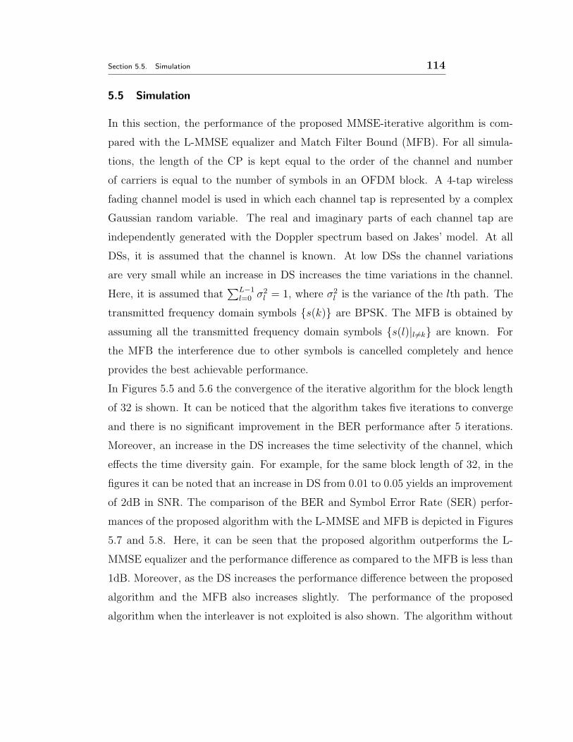
Section 5.5. Simulation 114
5.5 Simulation
In this section, the performance of the proposed MMSE-iterative algorithm is com-
pared with the L-MMSE equalizer and Match Filter Bound (MFB). For all simula-
tions, the length of the CP is kept equal to the order of the channel and number
of carriers is equal to the number of symbols in an OFDM block. A 4-tap wireless
fading channel model is used in which each channel tap is represented by a complex
Gaussian random variable. The real and imaginary parts of each channel tap are
independently generated with the Doppler spectrum based on Jakes’ model. At all
DSs, it is assumed that the channel is known. At low DSs the channel variations
are very small while an increase in DS increases the time variations in the channel.
Here, it is assumed that∑L−1
l=0 σ2l = 1, where σ2
l is the variance of the lth path. The
transmitted frequency domain symbols {s(k)} are BPSK. The MFB is obtained by
assuming all the transmitted frequency domain symbols {s(l)|l 6=k} are known. For
the MFB the interference due to other symbols is cancelled completely and hence
provides the best achievable performance.
In Figures 5.5 and 5.6 the convergence of the iterative algorithm for the block length
of 32 is shown. It can be noticed that the algorithm takes five iterations to converge
and there is no significant improvement in the BER performance after 5 iterations.
Moreover, an increase in the DS increases the time selectivity of the channel, which
effects the time diversity gain. For example, for the same block length of 32, in the
figures it can be noted that an increase in DS from 0.01 to 0.05 yields an improvement
of 2dB in SNR. The comparison of the BER and Symbol Error Rate (SER) perfor-
mances of the proposed algorithm with the L-MMSE and MFB is depicted in Figures
5.7 and 5.8. Here, it can be seen that the proposed algorithm outperforms the L-
MMSE equalizer and the performance difference as compared to the MFB is less than
1dB. Moreover, as the DS increases the performance difference between the proposed
algorithm and the MFB also increases slightly. The performance of the proposed
algorithm when the interleaver is not exploited is also shown. The algorithm without

Section 5.5. Simulation 115
the interleaver outperforms the L-MMSE equalizer, but it is poor when compared to
the MFB.
For the OFDM block length of 64, Figures 5.9 and 5.10 compare the BER and SER
performances of the iterative algorithm with the L-MMSE and MFB. As compared
to the block length of 32, more extrinsic information is available in the block length
of 64 to estimate any arbitrary transmitted symbol. Therefore, in the figures approx-
imately 2dB improvement in the SNR can be noticed.
To find the posteriori mean and variance of the frequency domain symbols, the pos-
teriori variance of the estimator, cov(s(k), s(k)), is required. By sacrificing some
performance gain, the computations of calculating the variance of estimator can be
saved. Therefore, if the variance of the estimator is supposed equal to one, it will
decrease the overall computational complexity. Figures 5.9 and 5.10 also show the
simulation results when Cov(s(k), s(k))|s(k) = 1 for all k. The performance gap is less
than 1dB.
Finally, Figure 5.11 shows the improvement in the BER performance, for a fixed value
of SNR, as the DS or the number of carriers in an OFDM block is increased.

Section 5.5. Simulation 116
0 5 10 1510
−4
10−3
10−2
10−1
SNR
BE
R
fd = 0.01
1st Iter.
2nd Iter.
3rd Iter.
4th Iter.
5th Iter.
Figure 5.5. Bit-error-rate performance of the MMSE-iterative algorithm after dif-
ferent numbers of iterations at DS of 0.01.
0 5 10 1510
−4
10−3
10−2
10−1
SNR
BE
R
fd = 0.05
1st Iter.
2nd Iter.
3rd Iter.
4th Iter.
5th Iter.
Figure 5.6. Bit-error-rate performance of the MMSE-iterative algorithm after dif-
ferent numbers of iterations at DS of 0.05.

Section 5.5. Simulation 117
0 5 1010
−4
10−3
10−2
10−1
BE
R
fd=0.001
0 5 1010
−4
10−3
10−2
10−1
SNR
fd=0.01
0 5 1010
−4
10−3
10−2
10−1
fd=0.05
MFBInterleavingNo InterleavingL−MMSE
Figure 5.7. BER performance comparison of the MMSE-iterative algorithm, after
five iterations and at different DSs, with the L-MMSE equalizer and MFB.
0 5 1010
−2
10−1
100
SE
R
fd=0.001
0 5 1010
−2
10−1
100
SNR
fd=0.01
0 5 1010
−2
10−1
100
fd=0.05
MFBInterleavingNo InterleavingL−MMSE
Figure 5.8. SER performance comparison of the MMSE-iterative algorithm, after
five iterations and at different DSs, with the L-MMSE equalizer and MFB.
Section 5.5. Simulation 118
0 2 4 6 8 10 1210
−4
10−3
10−2
10−1
BE
R
fd=0.001
MFBInterleavingLow complexity InterleavingNo InterleavingLow complexity no interleavingL−MMSE
0 2 4 6 8 10 1210
−4
10−3
10−2
10−1
SNR
fd=0.01
0 2 4 6 8 10 1210
−4
10−3
10−2
10−1
fd=0.05
Figure 5.9. BER performance comparison of the MMSE-iterative algorithm, after
five iterations and at different DSs, with the L-MMSE equalizer and MFB.
0 5 1010
−3
10−2
10−1
100
SE
R
fd=0.001
MFB
Interleaving
Low complexity Inter.
No Interleaving
Low complexity no inter.
L−MMSE
0 5 1010
−3
10−2
10−1
100
SNR
fd=0.01
0 5 1010
−3
10−2
10−1
100
fd=0.05
Figure 5.10. SER performance comparison of the MMSE-iterative algorithm, after
five iterations and at different DSs, with the L-MMSE equalizer and MFB.

Section 5.5. Simulation 119
0 0.02 0.04 0.06 0.08 0.110
−4
10−3
10−2
10−1
fd
BE
R
N = 8N = 16N = 32N = 64N = 128
Figure 5.11. Bit-error-rate performance using an MMSE-iterative algorithm after
five iterations at different DSs for different number of carriers in an OFDM block.

Section 5.6. Summary 120
5.6 Summary
In this chapter, the design of a low complexity OFDM iterative receiver, for a doubly
selective channel, was studied. The equalization was divided into two stages; the first
stage estimated the transmitted time domain symbols, with a length L MMSE equal-
izer, and then passed the estimated values to the second stage. In the second stage,
an FFT was applied on the estimated time domain symbols to convert them into the
frequency domain. Then, the means and variances of the transmitted frequency do-
main symbols were determined. The time domain means and variances were obtained
from the frequency domain means and variances using FFT and IFFT operations. In
order to obtain more accurate estimates, the time domain means and variances were
passed to the first stage to use in the following iteration. The first stage used these
values to update equalizer coefficient values and cancel the interference and provided
more accurate estimates. Thereby both stages iteratively exchanged their informa-
tion learnt from each other. To de-correlate the correlated outputs from both stages
an interleaver was introduced. The simulation results demonstrated the superior per-
formance of the proposed iterative scheme over the linear MMSE equalization, that
is not only computationally expensive but had poor performance. Importantly, the
new scheme had performance very close to the MFB. Moreover, unlike the iterative
method proposed in [19], the computational complexity of the proposed algorithm
was independent of DSs, and did not require any preprocessing and could work for a
large range of DSs, without increasing the computational complexity.

Section 5.7. Appendices 5 121
5.7 Appendices 5
Appendix 5A: Derivation of General MMSE Equalizer
From (5.2.6) it can be written as
rn = Hnx + vn,
to estimate time domain samples {x(n)}, the MMSE equalizer can be found by min-
imizing the cost function
J(wn) = E{|x(n) − wHn rn|2}
= E{x(n)x∗(n) − x(n)rHn wn − wH
n rnx∗(n) + wH
n rnrHn wn}. (5.7.1)
To minimize the cost function, J(wn), differentiate with respect to wn and equate to
zero to yield
E{rnx∗(n)} = E{rnr
Hn }wn (5.7.2)
E{(Hnx + vn)x∗(n)} = E{(Hnx + vn)(Hnx + vn)H}wn (5.7.3)
HnE{xx∗(n)} =(
E{HnxxHHHn + vnv
Hn })
wn (5.7.4)
HnCov[x(n), x(n)]in =(
HnE{xxH}HHn + E{vnv
Hn })
wn (5.7.5)
hncx(n) = [HnCov(x,x)HHn + σ2
vIL]wn (5.7.6)
and therefore the equalizer coefficient vector can be determined as
wn = (Hndiag(cx)HHn + σ2
vIL)−1hncx(n)
Section 5.7. Appendices 5 122
Appendix 5B: Derivation of General Estimator
The samples {x(n)} can be estimated by
x(n) = wHn rn (5.7.7)
and the expected value of the estimator can be written as
E{x(n)} = wHn Hnx (5.7.8)
If the estimator is unbiased then E{x(n)} = x(n), therefore, subtracting (5.7.8) from
(5.7.7) yields
x(n) = x(n) − wHn (rn − Hnx) (5.7.9)
Chapter 6
ITERATIVE EQUALIZATION FOR A
SINGLE CARRIER WITH CYCLIC
PREFIX SCHEME
OFDM is an attractive technique for achieving high bit rate transmission over wireless
channels and provides low complexity channel equalization over severe time invariant
multipath environments [89, 90]. However, an OFDM signal has very high Peak to
Average Power Ratio (PAPR) that has limited its application, since high PAPR re-
quires an expensive transmitter power amplifier [91]. In the worst case scenario, peak
transmitted power may be up to N times the average power, where N is the num-
ber of subcarriers used to transmit the OFDM block [92]. These large peaks cause
saturation in power amplifiers. The conventional methods to reduce the PAPR are
to use a linear power amplifier or back off the operating point of a non-linear power
amplifier. Both of these methods result in a significant power efficiency penalty. To
reduce PAPR the work in [91, 93] deliberately clips the OFDM signal before ampli-
fication, which mitigates the PAPR but introduces some performance degradation.
Cimini in [94,95] has presented a suboptimal strategy to tackle this problem.
Single Carrier with Cyclic Prefix (SCCP) is a closely related transmission scheme that
possesses most of the benefits of OFDM but does not have PAPR problem, thereby
eliminating the need for an expensive transmitter power amplifier that can operate
123

Section 6.1. A Brief Overview of the SCCP System 124
linearly over a wide range of signal amplitudes. On top of that the use of single carrier
transmission has several attractive features, which are given below [76,90,96]:
1. When combined with CP, its performance with FDE is similar to that of OFDM,
even for very long channel delay spread.
2. Single carrier modulation is a well proven technology in many existing wireless
and wire-line applications and its radio frequency requirements are well known.
Therefore, this chapter provides the application of iterative algorithm, presented in
the last chapter for OFDM, for SCCP systems.
6.1 A Brief Overview of the SCCP System
The basic baseband model of a conventional SCCP transmission and reception system
is shown in Figure 6.1. Here, similar to OFDM, the data are transmitted in blocks
and a CP is appended at the beginning of each data block. By doing this the effects of
IBI are completely removed. Moreover, for an SCCP system, this approach enables
the receiver to use the FFT and IFFT for FDE [86]. The data block is passed
through a PTS stage to transmit the symbols serially. At the receiver N + L −1 successive samples are collected and passed through an STP stage. Then, the
first L − 1 received samples are removed that contribute to the symbols from the
previous block. In FDE, the received time samples are converted into frequency
domain and an MMSE equalization is performed to estimate the frequency domain
transmitted symbols. If the channel is LTI then due to the presence of a diagonal
ICI matrix the computational complexity of the equalization is O(N). To obtain
the transmitted time domain symbols an inverse FFT is performed on the estimated
frequency domain symbols. The relationship between the time and frequency domain
symbols is given in (5.2.1). However, similar to OFDM an SCCP system is very
sensitive to time selectivity of the channel that disturbs the orthogonality of the ICI
matrix. For FDE, the time selectivity increases the computational complexity and

Section 6.2. Problem Statement 125
l
PT
S
ST
P
FFT
LTIChannel
x(0)x(1)
x(N-1)
x(N-L+1)
x(n) r(n)
r(0)
r(N-L+1)
r(1)
IFFT
ˆ (0)x
ˆ (1)x
x
FDE
(N-1)(N-1)
s
ˆ(0)s
Figure 6.1. A basic baseband SCCP scheme, transmitting subsequent blocks of N
data symbols and the receiver is performing frequency domain equalization, where L
is the support of channel.
decreases the BER performance due to the emergence of the off diagonal terms in the
ICI matrix. FDE for SCCP in a frequency selective channel is discussed in [76,90,97].
In most of the algorithms given in these papers, it is assumed that the channel is
only frequency selective. In order to perform FDE in SCCP systems operating over a
doubly selective channel, Schniter et al. [88], pre-processed the time domain received
signal by multiplying with window coefficients that squeeze the significant coefficients
in the ICI matrix into the 2D+1 central diagonals. Here, it is found thatD = fdN+1,
where fd is the DS due to the relative motion between the transmitter and receiver
and N is the number of symbols used to transmit an SCCP block of data. The
complexity of this algorithm increases as the DS increases. In contrast to this work,
as discussed in previous chapter, examining the time domain model of the received
SCCP signal too reveals that the CCM is already sparse and has similar structure to
that after preprocessing of the received samples [19,88].
6.2 Problem Statement
The iterative SCCP communication system used in this chapter is given in Figure
6.2. Before deriving the receiver, an intuitive explanation of its operation is discussed.
Initially, all data to be transmitted are converted into blocks and a CP is added in
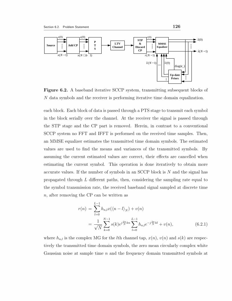
Section 6.2. Problem Statement 126
Source Add CPPTS
LTVChannel
STP&
DiscardCP
(0)x (0)x
MMSEEqualizer
Up-datePriors
ˆ(0)x
ˆ( 1)x N −( 1)x N L+ −
(0)x
(0)r
diag( )xc
( 1)x N − ( 1)r N −
( 1)x N −
Figure 6.2. A baseband iterative SCCP system, transmitting subsequent blocks of
N data symbols and the receiver is performing iterative time domain equalization.
each block. Each block of data is passed through a PTS stage to transmit each symbol
in the block serially over the channel. At the receiver the signal is passed through
the STP stage and the CP part is removed. Herein, in contrast to a conventional
SCCP system no FFT and IFFT is performed on the received time samples. Then,
an MMSE equalizer estimates the transmitted time domain symbols. The estimated
values are used to find the means and variances of the transmitted symbols. By
assuming the current estimated values are correct, their effects are cancelled when
estimating the current symbol. This operation is done iteratively to obtain more
accurate values. If the number of symbols in an SCCP block is N and the signal has
propagated through L different paths, then, considering the sampling rate equal to
the symbol transmission rate, the received baseband signal sampled at discrete time
n, after removing the CP can be written as
r(n) =L−1∑
l=0
hn,lx(〈n− l〉N) + v(n)
=1√N
N−1∑
k=0
s(k)ej 2πN
kn
L−1∑
l=0
hn,le−j 2π
Nkl + v(n), (6.2.1)
where hn,l is the complex MG for the lth channel tap, x(n), v(n) and s(k) are respec-
tively the transmitted time domain symbols, the zero mean circularly complex white
Gaussian noise at sample time n and the frequency domain transmitted symbols at

Section 6.2. Problem Statement 127
frequency k. By assuming the perfect knowledge of CIR, the N received samples in
vector form can be written as
r = Hx + v = HFHs + v. (6.2.2)
For FDE, the received time domain sample vector, r, is multiplied with the FFT
matrix that yields the frequency domain samples
Fr = FHFHs + Fv = Hdfs + Fv, (6.2.3)
where H is the CCM of size N ×N , the nth row and lth column entry of the matrix
H can be written as Hn,l = hn,〈n−l〉N . Similarly, as defined in the previous chapter, F
is the FFT matrix of size N ×N , Hdf is the ICI matrix and s is a vector of frequency
domain transmitted symbols. The MMSE equalizer for the estimation of s can be
found by minimizing E{‖s − WFr‖2} yielding
W = (HHdfHdf + σ2
nIN)−1HHdf (6.2.4)
where W is an equalizer coefficient matrix to decode all the frequency domain trans-
mitted symbols and σ2n is the variance of the noise. For frequency domain equalization,
if in (6.2.3) the channel is LTI then the matrix Hdf will be diagonal. Thereby, in or-
der to estimate the sequence of samples {s(k)}, the L-MMSE equalizer requires the
inversion of a diagonal matrix that is computationally inexpensive. Furthermore, to
estimate the sequence of transmitted symbols {x(n)}, an IFFT is performed on the
sequence of estimated samples {s(k)}.On the other hand, in a LTV channel the matrix H is not circulant, therefore the
matrix Hdf is not diagonal, a consequence of which is that ICI is introduced. Hence
the L-MMSE equalizer requires the inversion of an N ×N matrix that needs O(N2)
operations, which is infeasible for large N and yields poor BER performance [83].
However, as shown in Figure 5.4, if modulo-N indexing is assumed, then the struc-
ture of H reveals that the individual symbol x(n) contributes only to the observation

Section 6.3. Symbol Estimation 128
samples r(n) to r(n + L − 1). Therefore, considering modulo-N indexing in the se-
quel, it can be noted that these are the only samples required to estimate x(n) and
in vector form these received samples can be written as,
rn = Hnx + vn, (6.2.5)
where
rn =[
r(n) r(n+ 1) · · · r(n+ L− 1)]T
,
matrix Hn contains L rows of the matrix H from n to n+ L− 1 and
vn =[
v(n) v(n+ 1) · · · v(n+ L− 1)]T
.
6.3 Symbol Estimation
Similar to OFDM in the last chapter, to estimate the transmitted time domain sym-
bols, the sparsity present in the CCM is exploited to design a length L MMSE equal-
izer. As discussed in Chapter 5, in OFDM the time domain transmitted symbols have
a high number of unknown constellation points as a consequence of the IFFT opera-
tion on the symbols to be transmitted. Therefore, it was impractical to find the LLRs
of the time domain samples and frequency domain samples were obtained in order
to find the LLRs. In contrast, in SCCP, the transmitted time domain symbols have
finite constellation points. Therefore, the LLRs can be found without using frequency
domain samples. On this basis, next a low complexity MMSE-iterative algorithm is
described.
6.3.1 MMSE Equalizer
To find the MMSE equalizer for an SCCP system, the derivations of the previous chap-
ter are followed. The noise is assumed temporally uncorrelated, circularly distributed
and zero mean, therefore E{vn} = 0, E{vnvnH} = σ2
nIL and E{x(n)vn} = 0. Fur-
ther, define x(n) = E{x(n)}, x = E{x}, cx = [ cx(0) cx(1) · · · cx(N − 1) ] and

Section 6.3. Symbol Estimation 129
cx(n) = Cov[x(n), x(n)]. The MMSE equalizer, wn, of length L for the soft estimates
of x(n) can be derived by minimizing the cost function,
J(wn) = E{|x(n) − wHn rn|2}, (6.3.1)
which yields the MMSE equalizer coefficient vector, wn, and estimator x(n) as derived
in Appendix 5A and 5B,
wn =(
Hndiag(cx)HHn + σx
2IL
)−1hncx(n) (6.3.2)
x(n) = x(n) + wHn (rn − Hnx) (6.3.3)
with the assumption that {x(n) 6= 0}, the mean values of the estimates of the in-
dividual symbols can not be equal to zero, in (6.3.2) hn is the nth column of Hn.
For better estimates the a posteriori mean values {x(k)} can be found to cancel their
effects when finding any particular transmitted symbol. The posteriori mean values
require the a posteriori probabilities, which are found in the next section.
6.3.2 Iterative Algorithm
For better estimates, it is intended to determine the a posteriori values of {x(n)} and
{cx(n)} to use in (6.3.2) and (6.3.3) in the next iteration. To find these values the
following steps are required to form the proposed iterative algorithm.
Step 1: In the first iteration, all mean values are initialized to zero i.e. {x(n)} = 0
that corresponds to diag(cx) = IN , then, the estimate x(n) is obtained using (6.3.2)
and (6.3.3).
Step 2: As mentioned in the previous chapter, with the assumption of BPSK signals,
it is more convenient to work with the LLRs rather than the probabilities [98]. The
a priori and a posteriori LLRs of x(n) are defined as
L[x(n)] = ln(Pr{x(n) = 1}Pr{x(n) = −1}) (6.3.4)

Section 6.3. Symbol Estimation 130
and
L[x(n)|x(n)] = ln(Pr{x(n) = 1|x(n)}Pr{x(n) = −1|x(n)})
. (6.3.5)
The difference between the a posteriori and a priori LLRs (which is the extrinsic
information) of x(n), as derived in the previous chapter, is
△L[x(n)] = L[x(n)|x(n)] − L[x(n)] = L[x(n)|x(n)]
= lnp{x(n)|x(n)=1}p{x(n)|x(n)=−1}
. (6.3.6)
In order to find the extrinsic LLR, L[x(n)|x(n)], it is assumed that the probability
density function (PDF) of x(n) is Gaussian with variance σ2x and can be written as
p{x(n)} =1√
2πσx
exp
(
−(x(n) − E{x(n)})(x(n) − E{x(n)})H
2σ2x
)
. (6.3.7)
Therefore the conditional PDF, when the transmitted signal x(n) = b ǫ {+1,−1}, of
x(n) becomes
p{x(n)|x(n)=b} =1√
2πσx
exp
(
−(x(n) −mn(b))(x(n) −mn(b))H
2σ2x|x(n)=b
)
, (6.3.8)
where mn(b) = E{x(n)|x(n)=b} and σ2x|x(n)=b = Cov[x(n), x(n)|x(n)=b], which are the
conditional mean and variance of x(n).
Throughout the iterative receiver process, to estimate x(n) only the extrinsic infor-
mation is used. Which implies that, when estimating x(n), the a priori information is
set as x(n) = 0 and cx(n) = 1 in equations (6.3.2) and (6.3.3). Hence, the conditional

Section 6.3. Symbol Estimation 131
mean can be determined by using (6.3.3) as
E{x(n)|x(n)=b} = E{
x(n) + wHn (rn − Hnx)
}
|x(n)=b
= wHn Hn
x(0)
. . .
b+ x(n) − x(n)
. . .
x(N)
− wHn Hnx
= wHn Hninb+ wH
n Hnx − wHn Hnx
= wHn hnb (6.3.9)
It should be noted that mn(b) depends on the particular value of b. Similarly, it can
be shown that the conditional variance of x(n) becomes
σ2x|x(n)=b = E{x(n)xH(n)|x(n)=b} −mn(b)mn(b)H
= E{x(n)xH(n)|x(n)=b} − wHn hnh
Hn wn (6.3.10)
within which the term
E{x(n)xH(n)|x(n)=b} = wHn (Hndiag(cx)H
Hn + σ2
nIL)wn|x(n)=b (6.3.11)
Substituting (6.3.2) in (6.3.11) yieldsE{x(n)xH(n)|x(n)=b} = wHn hn. Therefore (6.3.10)
becomes
σ2x|x(n)=b = wH
n hn − wHn hnh
Hn wn. (6.3.12)

Section 6.3. Symbol Estimation 132
Note that unlike the mean the variance of the estimator is independent of b, and the
difference between the a posteriori and the a priori LLR of x(n) becomes
△L [x(n)] = ln
[
exp(
− (x(n)−mn(+1))2
σ2x|x(n)=+1
)]
[
exp(
− (x(n)−mn(−1))2
σ2x|x(n)=−1
)]
= −(x(n) − wHn hn)2
σ2x|x(n)=+1
+(x(n) + wH
n hn)2
σ2x|x(n)=−1
= 4Re{x(n)}1 − hH
n wn
. (6.3.13)
Therefore, the a posteriori LLR of x(n)
L[
x(n)|x(n)
]
= L [x(n)] + △L [x(n)] . (6.3.14)
Step 3: Exploiting (6.3.14) and using the property Pr{x(n) = 1|x(n)} +
Pr{x(n) = −1|x(n)} = 1 the posteriori values for x(n) and cx(n) are obtained as
x(n)|x(n) = Pr{
x(n) = +1|x(n)
}
− Pr{
x(n) = −1|x(n)
}
= tanh
(
L[
x(n)|x(n)
]
2
)
(6.3.15)
and
cx(n)|x(n) =∑
bǫ{+1,−1}(b− x(n)|x(n))
2Pr(x(n) = b|x(n))
= 1 − x(n)|2x(n). (6.3.16)
Note that equations (6.3.15) and (6.3.16) update the values of x(n) and cx(n) in
(6.3.2) and (6.3.3) in Step 1.
Step 4: Steps 1 to 3 are repeated until the specified number of iterations has elapsed.
The Table 6.1 shows the overall iterative algorithm used for the simulations.

Section 6.4. Complexity of the Algorithm 133
Table 6.1. MMSE-Iterative algorithm for SCCP
L = zeros(N, 1)
x = zeros(N, 1)
diag(cx) = IN
while iter ≤ max− iter
for n = 1 : N
x(n) = 0 ; cx(n) = 1
wn = (Hndiag(cx)HHn + σ2I)−1hn
x(n) = x(n) + wH(rn − Hnx)
△L(k) = 4Re{x(n)}1−hH
n wn
L(k) = L(k) + △L(k)
x(n) = tanh(L(k)/2)
cx(n) = 1 − x(n)2
end
6.4 Complexity of the Algorithm
6.4.1 Linear Time Variant Channel
In each iteration, to find the equalizer coefficient values wn, the algorithm requires
the inversion of [Hndiag(cx)HHn + σ2
nIL] that needs O(L2) operations and must be
performed N times per iteration. Although the dimensions of matrix Hn are L ×N , it contains only 2L − 1 non-zero columns. The product term inside the matrix
Hndiag(cx)HHn can be computed in O(L2) operations as a consequence of the sparsity
within the channel convolution matrix. Once wn is obtained the estimation of x(n)
requires the computation of Hnx that also needs O(L2) operations and must be
repeated N times per iteration. Therefore, to estimate N symbols only O(NL2)
computations per iteration are required.

Section 6.5. Simulation 134
6.4.2 Linear Time Invariant Channel
In an LTI channel the FDE requires O(2N log2N) operations, while the proposed
algorithm requires O(L2N) operations per iteration. Therefore, the complexity of the
proposed algorithm for a small length of channel (≤5) is identical to the complexity
of the FDE but the performance is better.
6.5 Simulation
In this section, the performance of the proposed low complexity MMSE-iterative
algorithm is compared with the L-MMSE equalizer and MFB. The length of the CP
is kept equal to the length of the channel. A 4-tap wireless fading channel model is
used in which each channel tap is represented by a complex Gaussian random variable.
The real and imaginary parts of each channel tap are independently generated with
the Doppler spectrum based on Jakes’ model. Here, it is assumed that∑L−1
l=0 σ2l =
1, where σ2l is the variance of the lth path. The transmitted symbols {x(n)} are
BPSK. The MFB is obtained from the model given in (6.2.2) by assuming the symbols
{x(l)|l 6=n} are known. In Figures 6.3 and 6.4 respectively, the convergence of the
proposed iterative algorithm is analyzed for slow and fast time varying channels, for
the SCCP block length of 32. From the figures it can be seen that the algorithm
converges after five iterations and there is no significant change after five iterations.
Moreover, for fast time varying channels it converges slightly faster. Figures 6.5 and
6.6 respectively compare the BER and SER performance of the iterative algorithm
with the L-MMSE equalizer and MFB for the SCCP block length of 32. At low
DS, for example fd = 0.001, the channel changes very slowly and in this case the
performances of the iterative method and the L-MMSE equalizer are close to each
other. However, as the large DS introduces significant time selectivity into the channel
the proposed algorithm outperforms the L-MMSE equalizer. Figure 6.7 repeats the
simulation in Figure 6.5 for the SCCP block length of 64. By comparing the results
of these figures, it can be concluded that using long length SCCP blocks of data

Section 6.5. Simulation 135
appears to yield better performance. For example, considering the performance of
the iterative algorithm for the SCCP block length of 32 and 64 for the DS of 0.05. The
algorithm for the SCCP block length of 64 yields 1dB gain in SNR. The reason for
this gain is due to the fact that to estimate a symbol x(n), more extrinsic information
is available. In Figure 6.8, the performance of the proposed algorithm is compared
with the FDE for the case of an LTI channel. Even in the case of an LTI channel,
the iterative method outperforms the FDE by at least 1dB.

Section 6.5. Simulation 136
0 5 10 1510
−4
10−3
10−2
10−1
SNR
BE
R
fd = 0.001
1st Iter.
2nd Iter.
3rd Iter.
4th Iter.
5th Iter.
6th Iter.
7th Iter.
8th Iter.
9th Iter.
10th Iter.
Figure 6.3. BER performance of the iterative algorithm after different number of
iterations at slow fading fd = 0.001.The number of symbols in a SCCP block is 32.
0 5 10 1510
−4
10−3
10−2
10−1
SNR
BE
R
fd = 0.05
1st Iter.
2nd Iter.
3rd Iter.
4th Iter.
5th Iter.
6th Iter.
7th Iter.
8th Iter.
9th Iter.
10th Iter.
Figure 6.4. BER performance of the iterative algorithm after different number of
iterations at fast fading fd = 0.05. The number of symbols in a SCCP block is 32.

Section 6.5. Simulation 137
0 5 10 1510
−4
10−3
10−2
10−1
BE
R
fd=0.001
MFBIterativeFDE
0 5 10 1510
−4
10−3
10−2
10−1
SNR
fd=0.01
0 5 10 1510
−4
10−3
10−2
10−1
fd=0.05
Figure 6.5. Bit error rate performance comparison of the proposed iterative algo-
rithm after five iterations with the L-MMSE equalizer and MFB at different DSs.
The number of symbols in one block is 32 and the length of the channel is 4.
0 5 10 1510
−3
10−2
10−1
100
SE
R
fd=0.001
MFB
Iterative
FDE
0 5 10 1510
−3
10−2
10−1
100
SNR
fd=0.01
0 5 10 1510
−3
10−2
10−1
100
fd=0.05
Figure 6.6. Symbol error rate performance comparison of the proposed iterative
algorithm after five iterations with the L-MMSE equalizer and MFB at different DSs.
The number of symbols in one block is 32 and the length of the channel is 4.

Section 6.5. Simulation 138
0 5 10 15
10−4
10−3
10−2
10−1
fd = 0.01
BE
R
FDEIterativeMFB
0 5 10 15
10−4
10−3
10−2
10−1
fd = 0.05
SNR0 5 10 15
10−4
10−3
10−2
10−1
fd = 0.1
Figure 6.7. BER performance comparison of the proposed iterative algorithm after
five iterations with the L-MMSE equalizer and MFB at different DSs. The number
of symbols in one block is 64 and the length of the channel is 4.
0 2 4 6 8 10 12
10−3
10−2
10−1
SNR
BE
R
FDE5th−IterMFB
Figure 6.8. BER performance comparison of the proposed iterative algorithm for
an LTI channel after five iterations with the FDE and MFB. In both equalizations,
the number of symbols in one block is 32 and the length of the channel is 4.

Section 6.6. Summary 139
6.6 Summary
In this chapter the design of a low complexity iterative SCCP receiver for LTV and LTI
channels has been considered. The proposed algorithm exploits the sparsity present
in the CCM to design a length L MMSE equalizer. In contrast to FDE, the proposed
algorithm does not involve the IFFT and FFT operations. The simulation results
demonstrate the superiority of the proposed scheme over the L-MMSE equalizer,
which is not only computationally expensive but has poor performance. On the other
hand, unlike the iterative method proposed in [88], the computational complexity
of the proposed algorithm is independent of DS, does not require preprocessing and
can work for a large range of DSs without increasing the computational complexity
significantly. The computational complexity of the proposed algorithm depends on the
length of the channel that can be reduced by applying channel shortening algorithms.

Chapter 7
CONCLUSION AND FUTURE
WORK
7.1 Conclusion
With the advent of multimedia services in mobile communication the demand for
high data rate is continuously increasing. High data rate transmission on a bandlim-
ited channel gives rise to ISI, the effects of which can be mitigated by employing
an equalizer at the receiver. On the other hand, for high data rate transmission
the signals are transmitted on very high frequencies that in a mobile environment
introduces significant DSs in the carrier frequencies, which is one of the main rea-
sons for time variations in frequency selective channels. Time variation in frequency
selective channels degrades the BER performance of communication systems and in-
creases the computational burden on the receiver. In fast time-varying channels with
higher order modulation schemes, adaptive equalizers may not perform well. There-
fore, block based equalizers are preferred but they require the channel parameters.
In fast time-varying channels the estimation of channel parameters becomes a chal-
lenging problem. Therefore, in this thesis the parameter estimation and equalization
techniques for doubly selective channels have been developed and analyzed.
This thesis started with a simple time-varying deterministic channel, where the rela-
tive motion between the transmitter and receiver was very high and various multipaths
experienced different DSs due to different angle of arrival. Distinct DSs introduced
140

Section 7.1. Conclusion 141
sinusoidal time-variations in each multipath of the channel. At first, the equalization
of a wireless SISO channel that allowed multipath with distinct DSs was considered.
For this scenario, to mitigate the effects of the channel, the equalizer coefficient val-
ues required the knowledge of CSI and FOs. To estimate the FOs using MLE was an
L dimensional maximization problem, where L is the support of the channel. How-
ever, exploiting the correlation property of the transmitted training sequence the L
dimensional maximization problem was split into L one dimensional maximization
problems. To validate the performance of FOs and CSI estimators, the CRLB was
derived and the performance of the estimators was compared with this bound. The
estimators were found to be statistically efficient. Moreover, distinct FOs could not
be compensated for prior to equalization (as in conventional equalizations), therefore,
they were accounted for in the equalizer design. By doing this, the equalizer design
required the inversion of an M ×M matrix to decode each symbol, where M was
the number of equalizer taps. To reduce the computational burden on the receiver, a
novel equalization structure was proposed that exploited the deterministic structural
movements of the matrices in CCM, using matrix inversion lemmas and a corollary
derived from these matrix inversion lemmas. The proposed algorithm did not require
the inversion of an M×M matrix, rather the inversion of an (M−1)×(M−1) matrix
was performed only at the start of the frame, for rest of the symbols no inversion was
required.
Then the equalization of a SISO channel with multipath and multiple FOs was ex-
tended for multi-user transmission systems where the channel was modelled as a
multiple-input and multiple-output frequency selective system. Here, estimation of
FOs was an nRL dimensional problem. But due to uncorrelated training symbols from
each transmit antenna, the problem was split into nRL one dimensional maximization
problems. Here, again due to distinct DSs, the equalizer required the inversion of an
nRM × nRM matrix. But, exploiting the structural movements of the matrices as
in the SISO system the computational complexity was reduced significantly. In this
Section 7.1. Conclusion 142
case, at the start of the frame the inversion of a (M − 1)nR × (M − 1)nR matrix was
required, but for rest of the symbols in the frame, only the inversion of an nR × nR
matrix was required.
In the rich scattering environment or when there was motion of physical objects
between the transmitter and the receiver, the CCM did not change deterministically
and the structural movements of the matrices could not be seen. In this scenario the
channel was assumed to follow the Rayleigh fading model. Therefore, in the next
step, the equalization of a general doubly selective channel was studied. For the
equalization of a doubly selective channel, an OFDM scheme was considered, since
it is more sensitive to the time selectivity of the channel. Here, it was assumed that
the channel was known at the receiver. In OFDM, a time-varying channel intro-
duced ICI that increased the computational complexity to O(N3) and degraded the
BER performance of the receiver. For an OFDM doubly selective channel, using the
time and frequency samples a low complexity iterative algorithm was proposed. This
algorithm exploited the sparsity present in the CCM to design a length L MMSE
equalizer to decode the transmitted time domain samples, where L was the number
of multipaths. The time domain samples were estimated on the basis of interference
cancellations. Here, the time domain samples did not have finite constellation due
to the IFFT operation therefore, it was difficult to find the mean values. In order to
find the mean values, the estimated time domain samples were passed to the second
stage where the frequency domain symbols were found. As the frequency domain
symbols had finite constellations, it was easy to find the mean values. Mean val-
ues obtained in the second stage were converted into the time domain and passed
back to the first stage. Both of these stages shared their information learnt from
each other iteratively and worked independently. To make the outputs of each stage
independent of each other, a random interleaver and a de-interleaver were introduced.
Section 7.2. Future Work 143
Finally, the iterative equalization of a Rayleigh fading channel for a SCCP system
was considered. In contrast to the equalization of an OFDM channel, this algorithm
worked only with time domain samples. In an SCCP system, at the transmitter no
IFFT is performed on the signals to be transmitted, therefore, the transmitted time
domain samples have finite constellations. In the proposed algorithm for SCCP, at
the receiver, in contrast to conventional FDE, no FFT and IFFT was performed.
To estimate the time domain samples a length L MMSE equalizer is designed and
time domain samples were obtained by cancelling the interfering symbols obtained
in the previous iteration. From the estimated time domain symbols the a posteriori
probabilities were found and used to find the a posteriori means of the transmit-
ted symbols. In the following iteration these mean values were used to cancel the
interfering symbols when estimating symbols for obtaining more accurate values.
7.2 Future Work
The work presented in this thesis can be extended in a number of directions, includ-
ing specific issues related to the algorithms presented. The proposed low complex-
ity equalization presented in first two contribution chapters can be extended to the
DFE, wherein, exploiting the structural movement in the convolution matrix could
be challenging, but the DFE could provide a much better performance. Moreover,
the presented FO estimation and correction can be employed in Ultra Wide Band
(UWB), where the problem is more challenging due to wide spectrum of the signal.
In the last two chapters iterative algorithms are presented and a critical issue of
estimation of time-varying channels was ignored. In our on-going work, the estima-
tion of time-varying channels is being considered.
The proposed iterative algorithms also resemble turbo equalization, in on-going work
the performance gap between the turbo equalization and the proposed algorithm when

Section 7.2. Future Work 144
coding is applied is being considered.
Here, the computational complexity of the algorithm increases linearly with the length
of the channel. This can limit the application of the algorithm only to small length
channels. In on-going work, it is being tried to develop algorithms that do not in-
crease the computational complexity linearly with the channel length. Time domain
channel shortening algorithms for doubly selective channels can also be found.
The work of iterative equalization could also be extended to MIMO OFDM.

BIBLIOGRAPHY
[1] S. Ahmed, S. Lambotharan, A. Jakobsson, and J. A. Chambers, “Parameter esti-
mation and equalization techniques for communication channels with multi-path and
multiple frequency offsets,” IEEE Trans. Commun., vol. 53, pp. 219–223, Feb. 2005.
[2] S. Ahmed, S. Lambotharan, A. Jakobsson, and J. A. Chambers, “MIMO frequency
selective channels with multiple frequency offsets: Estimation and detection tech-
niques,” IEE Commun. Proceedings, pp. 489– 494, Aug. 2005.
[3] S. Ahmed, S. Lambotharan, A. Jakobsson, and J. A. Chambers, “Parameter Es-
timation and Equalization Techniques for MIMO Frequency Selective Channels with
Multiple Frequency Offsets,” European Signal Processing Conference, Vienna, Aus-
tria, Sep. 2004.
[4] S. Ahmed, S. L. M. Sellathurai, and J. A. Chambers, “Low Complexity Iterative
Method of Equalization for OFDM in wireless channels with Multiple Frequency
Offsets,” European Signal Processing Conference, Antalya, Turkey, Sep. 2005.
[5] S. Ahmed, M. Sellathurai, and J. A. Chambers, “Low complexity iterative method
of equalization for OFDM in doubly selective channels,” sumitted to IEEE Trans.
Wireless Commun., Jul. 2005.
[6] S. Ahmed, M. Sellathurai, and J. A. Chambers, “Low complexity iterative method
of equalization for OFDM in time varying channels,” accepted for 39th Asilomar
145

Bibliography 146
Conference on Signals, Systems and Computers, Pacific Groves, California USA.,
Oct. 2005.
[7] S. Ahmed, M. Sellathurai, S. Lambotharan, and J. A. Chambers, “Parameter esti-
mation and equalization techniques for communication channels with multi-path and
multiple frequency offsets,” accepted for IEEE Signal Processing Letters.
[8] E. Ayanoglu, K. Y. Eng, M. J. Karol, Z. L. P. Pancha, M. Veeraraghavan, and
C. B. Woodworth, “Mobile Infra-structure,” Bell-Labs Technical Journal, pp. 143–
161, 1996.
[9] T. Ojanpera and R. Prasad, Wideband CDMA for Third Generation Mobile Com-
munications. Artech House, 1998.
[10] S. Ohmori, Y. Yamao, and N. Nakajima, “The future generation of mobile com-
munications based on broadband access technologies,” IEEE Commun. Magazines,
vol. 38, pp. 134–149, Dec. 2000.
[11] T. S. Rappaport, Wireless Communications Principles and Practice. Upper Saddle
River, N.J.: Prentice-Hall, 2002.
[12] R. Pirhonen, T. Rautava, and J. Penttinen, “TDMA convergence for packet data
services,” IEEE Personnel Communication Magazine, vol. 6, pp. 68–73, June 1999.
[13] M. Zeng, A. Annamalai, and V. K. Bargava, “Harmonization of third-generation
mobile systems,” IEEE Commun. Magazines, pp. 94–104, Dec. 2000.
[14] H. Holma and A. Toskala, WCDMA for UMTS. New York, N.Y.: John Wiley
and Sons, Inc., 2004.
[15] W. Mohr and W. Konhauser, “Access network evaluation beyond third generation
mobile communications,” IEEE Commun. Magazines, vol. 38, pp. 122–133, Dec. 2000.

Bibliography 147
[16] B. D. Woerner, J. H. Reed, and T. S. Rappaport, “Simulation issues for future
wireless modems,” IEEE Commun. Magazines, pp. 42 – 53, Jul. 1994.
[17] J. G. Proakis, Digital Communications. McGraw-Hill, Inc., 1989.
[18] S. Qureshi, “Adaptive equalization,” IEEE Proceedings, vol. 73, pp. 1349–1387,
Sep. 1985.
[19] P. Schniter, “Low-Complexity Equalization of OFDM in Doubly Selective Chan-
nels,” IEEE Trans. on Signal Processing, vol. 52, pp. 1002–1010, April 2004.
[20] H. Viswanathan and R. Krishnamoorthy, “A frequency offset estimation technique
for frequency selective fading channels,” IEEE Commun. Letters, vol. 5, pp. 166–168,
April 2001.
[21] P. Stoica and O. Besson, “Training sequence design for frequency offset and fre-
quency selective channel estimation,” IEEE Trans. Commun., vol. 51, pp. 1910– 1917,
Nov. 2003.
[22] K. E. Scott and E. B. Olasz, “Simultaneously clock phase and frequency offset
estimation,” IEEE Trans. Commun., vol. 43, pp. 2263–2270, July 1995.
[23] H. Murata and S. Yoshida, “Maximum-likelihood sequence estimation receiver
with joint frequency offset and delay profile estimation technique ,” Global Telecom-
munications Conference (GLOBECOM 98)., vol. 6, pp. 3455 – 3459, Nov. 1998.
[24] X. Cai and G. B. Giannakis, “ Low-complexity ICI Suppression for OFDM over
Time and Frequency-Selective Rayleigh Fading Channels ,” Asilomar Conference on
Signals, Systems and Computers, vol. 2, pp. 1822 – 1826, Nov 2002.
[25] S. Haykin, Communication Systems. John Wiley and Sons, Inc.
[26] W. C. Jakes, Microwave Mobile Communications. Wiley IEEE Press, May, 1994.
Bibliography 148
[27] C. Toker, “Signal Processing Algorithms and Architectures for Communication
Transceivers,” PhD thesis, University of London, Sep. 2004.
[28] M. Morelli, U. Mengali, and G. M. Vitetta, “Further results in carrier frequency
estimation for transmissions over flat fading channels,” IEEE Commun. Letters, vol. 2,
pp. 327–330, Dec. 1998.
[29] L. Krasny, H. Arslan, D. Koilpillai, and S. Chennakeshu, “Doppler spread esti-
mation for wireless mobile radio systems,” IEEE Commun. Letters, vol. 5, pp. 197 –
199, May 2001.
[30] S. M. Kay, Fundamentals of Statistical Signal Processing, Estimation Theory. En-
glewood Cliffs, N.J.: Prentice-Hall, 1993.
[31] A. Paulraj and C. Papadias, “Space time processing for wireless communications,”
IEEE Signal Processing Magazine, vol. 14, pp. 49–83, Nov. 1997.
[32] A. Naguib, N. Seshadri, and A. R. Calderbank, “Increasing data rate over wireless
channels,” IEEE Signal Processing Magazine, vol. 17, pp. 76–92, May 2000.
[33] O. Besson and P. Stoica, “On parameter estimation of MIMO flat-fading channels
with frequency offsets,” IEEE Trans. Signal Processing, vol. 51, pp. 602–613, March
2003.
[34] J. A. C. Bingham, ADSL, VDSL, and Multicarrier Modulation. New York: John
Wiley and Sons, Inc., 2000.
[35] T. Starr, J. M. Cioffi, and P. J. Silverman, Understanding Digital Subscriber Line
Technology. Upper Saddle River, N.J.: Prentice-Hall, 1999.
[36] R. W. Lucky, “Automatic equalization for digital Communication,” Bell System
Technical Journal, vol. 46, pp. 547–588, Nov. 1965.
Bibliography 149
[37] J. G. Proakis and J. Miller, “An adaptive receiver for digital signaling through
channels with inter-symbol-interference,” IEEE Trans. on Inform. Theory, vol. 15,
pp. 484–497, Jul. 1969.
[38] S. Qureshi, “Adaptive equalization,” IEEE Transaction on Signal Processing,
vol. 20, pp. 9–16, Mar. 1982.
[39] J. G. Proakis, “Adaptive equalization for TDMA digital mobile radio,” IEEE
Trans. on Vehicular Technology, vol. 40, pp. 333–341, May 1991.
[40] G. D. Forney, “The Viterbi algorithm,” IEEE Proceedings, vol. 61, pp. 268–278,
Mar. 1978.
[41] H. Chen, R. Perry, and K. Buckley, “On MLSE algorithms for unknown fast
time-varying channels,” IEEE Trans. Commun., vol. 51, pp. 730–734, May 2003.
[42] J. T. Chen, A. Paulraj, and U. Reddy, “Multichannel maximum-likelihood se-
quence estimation (MLSE) equalizer for GSM using a parametric channel model,”
IEEE Trans. Commun., vol. 47, pp. 53–63, Jan. 1999.
[43] “Multiplexing and multiple access on radio path,” 3GPP TS 45.002 (V5.9.0),
April 2003.
[44] V. D. Trajkovic, P. B. Rapajic, and R. A. Kennedy, “Low-complexity iterative
decoding with decision-aided equalization for magnetic recording channels,” To appear
in IEEE Signal Processing Letters.
[45] W. Zi-Ning and J. M. Cioffi, “Low-complexity iterative decoding with decision-
aided equalization for magnetic recording channels,” IEEE Journal on Selected Areas
in Commun, vol. 19, pp. 699 – 708, Apr. 2001.
[46] C. A. Belfiori and J. H. Park, “Decision feed-back equalizer,” IEEE Proc., vol. 67,
pp. 1143–1156, Aug. 1979.

Bibliography 150
[47] A. C. Raul, P. B. Schniter, J. Balakrishnan, and C. R. Johnson, “Tutorial on de-
cision feed-back equalizer,” (www.ece.osu.edu/schniter/research.html), pp. 1–20, Jul.
1998.
[48] B. Widrow and S. D. Stearns, Adaptive Signal Processing. Englewood Cliffs, N.J.:
Prentice-Hall, 1985.
[49] A. R. S. Bahai and M. Sarraf, “A frequency offset estimation technique for nonsta-
tionary channels,” International Conference on Acoustics, Speech, and Signal Process-
ing (ICASSP), vol. 5, pp. 3897 – 3900, April 1997.
[50] A. R. S. Bahai and M. Sarraf, “A frequency offset estimation technique for wireless
channels,” First IEEE Signal Processing Workshop on Signal Processing Advances in
Wireless Commun., pp. 397 – 400, April 1997.
[51] W. Y. Kuo and M. P. Fitz, “Frequency offset compensation of pilot symbol assisted
modulation in frequency flat fading,” IEEE Trans. Commun., vol. 45, pp. 1412 – 1416,
Nov. 1997.
[52] A. V. Oppenheim and R. W. Schafer, Discrete-Time Signal Processing. Prentice-
Hall, 1989.
[53] P. Stoica and R. Moses, Introduction to Spectral Analysis. Upper Saddle River,
N.J.: Prentice Hall, 1997.
[54] B. Porat, A Course in Digital Signal Processing. New York, N.Y.: John Wiley
and Sons, Inc., 1997.
[55] A. Eriksson, P. Stoica, and T. Soderstrom, “Asymptotical analysis of MUSIC and
ESPRIT frequency estimates,” IEEE International Conference on Acoustics, Speech
and Signal Processing (ICASSP), vol. 4, pp. 556 – 559, Apr. 1993.
[56] S. Haykin, Adaptive Filter Theory (2nd edition). Englewood Cliffs, N.J.: Prentice
Hall, Inc., 1991.
Bibliography 151
[57] G. Strang, Linear algebra and its applications, 3rd Ed. Thomson Learning, Inc,
1988.
[58] E. Serpedin, A. Chevreuil, G. B. Giannakis, and P. Loubaton, “Blind channel
and carrier frequency offset estimation using periodic modulation precoders,” IEEE
Trans. Signal Processing, vol. 48, pp. 2389–2405, Aug. 2000.
[59] Y. Ma and Y. Huang, “Blind estimation of carrier frequency offset for OFDM
in unknown multi-path channels,” IEE Electronics Letter, vol. 39, pp. 128–130, Jan.
2003.
[60] M. Ghogho and A. Swami, “Blind frequency-offset estimator for OFDM systems
transmitting constant-modulus symbols,” IEEE Commun. Letters, vol. 6, pp. 343 –
345, Aug. 2003.
[61] S. Haykin and M. Moher, Modern Wireless Communications. Upper Saddle River,
N. J.: Prentice Hall, Inc., 2005.
[62] D. K. Hong, Y. J. Lee, D. Hong, and C. Kang, “Robust frequency offset esti-
mation for pilot symbol assisted packet CDMA with MIMO antenna system,” IEEE
Commun. Letters, vol. 6, pp. 262–264, June 2002.
[63] L. Krasny, H. Arslan, D. Koilpillai, and S. Chennakeshu, “Optimal and suboptimal
algorithms for Doppler spread estimation in mobile radio systems,” IEEE Interna-
tional Symposium on Personal, Indoor and Mobile Radio Communications (PIMRC
2000), vol. 2, pp. 1295 – 1299, Sep. 2000.
[64] A. R. S. Bahai and M. Sarraf, “Frequency offset estimation in frequency selective
fading channels,” Vehicular Technology Conference (VTC), vol. 3, pp. 1719 – 1723,
May 1997.
[65] Markku, J. Heihhila, P. Komulainen, and J. Lilleberg, “Interference suppression in
Bibliography 152
CDMA downlink through adaptive channel equalization,” IEEE Vehicular Technology
Conference, 1999-Fall.
[66] T. Kailath and A. H. Sayed, Fast Reliable Algorithms for Matrices with Structure.
Philadelphia, USA: SIAM, 1999.
[67] M. A. Jensen and J. W. Wallace, “A review of antennas and propagation for
MIMO wireless communications,” IEEE Trans. Antennas and Propagation, pp. 2810–
2824, Nov. 2004.
[68] C. E. Shannon and W. Weaver, The Mathematical Theory of Communication.
Urbana: University of Illinois Press, 1962.
[69] J. Mietzner and P. A. Hoeher, “Boosting the performance of wireless communi-
cation systems: theory and practice of multiple-antenna techniques,” IEEE Commu-
nications Magazine, pp. 40 – 47, Oct. 2004.
[70] G. J. Foschini and M. G. Gans, “On limits of wireless communications in a fad-
ing environment when using multiple antennas,” Wireless Personal Communications,
pp. 311–335, Mar. 1998.
[71] I. E. Telatar, “Capacity of multi-antenna Gaussian channels,” European Transac-
tions on Telecommunications, pp. 585–595, Nov. 1999.
[72] G. J. Foschini, “Layered space-time architecture for wireless communication in a
fading environment when using multi-element antennas,” Bell Labs. Technical Jour-
nal, pp. 41–59, Autumn 1996.
[73] S. M. Alamouti, “A simple transmit diversity technique for wireless communica-
tions,” IEEE Transaction on Selected Areas in Communications, vol. 16, pp. 1451–
1458, Oct. 1998.

Bibliography 153
[74] V. Tarokh, H. Jafarkhani, and A. R. Calderbank, “Space time block codes from
orthogonal design,” IEEE Transactions on Information Theory, vol. 45, pp. 1456–
1467, July 1999.
[75] D. E. A. Clarke and T. Kanada, “Broadband: The last mile,” IEEE Commun.
Magazine, vol. 31, pp. 94–100, Mar. 93.
[76] H. Sari, G. Karam, and I. Jeanclaude, “Frequency domain equalization of mobile
radio and terrestrial broadcast channels,” In Proc. Globcom Conference, San Fran-
cisco, pp. 1–5, Nov. 1994.
[77] M. Morelli and U. Mengali, “An improved frequency offset estimator for OFDM
applications,” IEEE Commun. Letters, vol. 45, pp. 75–77, Mar. 1999.
[78] M. Morelli, “Timing and frequency synchronization for the uplink of an OFDMA
System,” IEEE Trans. Commun., vol. 52, pp. 296 – 306, Feb. 2004.
[79] J. J. Beek, P. O. Borjesson, M. L. Boucheret, D. Landstrom, J. M. Arenas, and
P. Odling, “A time and frequency synchronization scheme for multiuser OFDM,”
IEEE Journals on Selected Areas of Commun., vol. 17, pp. 1378 – 1389, Nov. 1999.
[80] J. C. Lin, “Maximum-likelihood frame timing instant and frequency offset esti-
mation for OFDM communication over a fast Rayleigh-fading channel,” IEEE Trans.
Vehicular Technology, vol. 52, pp. 1049 – 1062, July 2003.
[81] J. J. Beek, P. O. Borjesson, and M. Sandell, “Non-data-aided carrier frequency
offset estimation for OFDM and downlink DS-CDMA systems,” IEEE Trans. Signal
Processing, vol. 45, pp. 1800–1805, Jul. 1997.
[82] P. H. Moose, “A technique for orthogonal frequency division multiplexing fre-
quency offset correction,” IEEE Trans. Commun., vol. 42, pp. 2908–2914, Oct. 1994.

Bibliography 154
[83] Y. S. Choi, P. J. Voltz, and F. A. Cassara, “On Channel Estimation and Detection
for Multi-carrier Signals in Fast and Selective Rayleigh Fading Channels ,” IEEE
Trans. Commun, vol. 49, pp. 1375 – 1387, Aug 2001.
[84] Y. R. Zheng and C. Xiao, “Simulation models with correct statistical properties
for Rayleigh fading channels,” IEEE Trans. Commun., pp. 920–928, June. 2003.
[85] B. Sklar, “Rayleigh fading channels in mobile digital communication systems Part
II: Mitigation,” IEEE Commun. Magazine, vol. 35, pp. 102–109, Jul. 1997.
[86] G. L. Stuber, J. R. Barry, S. W. Mclaughlin, and M. A. Ingram, “Broadband
MIMO-OFDM wireless Commun.,” Proc. IEEE, vol. 92, pp. 271 – 294, Feb. 2004.
[87] M. Tuchler, R. Koetter, and A. C. Singer, “Turbo equalization: Principles and
new results,” IEEE Trans. Commun., vol. 50, pp. 754–766, May. 2002.
[88] P. Schniter and H. Liu, “Iterative Equalization for Single-Carrier Cyclic-Prefix in
Doubly-Dispersive Channels,” Asilomar Conference on Signals, Systems and Com-
puters, vol. 1, pp. 502 – 506, Nov. 2003.
[89] I. Koffman and V. Roman, “Broadband wireless access solutions based on OFDM
access in IEEE 802.16,” IEEE Communications Magazine, pp. 96–103, Apr. 2002.
[90] H. Sari, G. Karam, and I. Jeanclaude, “Transmission techniques for digital terres-
trial TV broadcasting,” IEEE Communications Magazine, vol. 33, pp. 100–109, Feb.
1995.
[91] X. Li and L. J. C. Jr., “Effects of clipping and filtering on the performance of
OFDM,” IEEE Commun. Lett., vol. 2, p. 131133, May 1998.
[92] M. E. R. Khan and K. M. Ahmed, “A novel technique for peak to average power
ratio reduction in OFDM systems,” Canadian Conference on Electrical and Computer
Engineering, vol. 1, pp. 165–168, May 1996.
Bibliography 155
[93] R. O. Neill and L. N. Lopes, “Envelope variations and spectral splatter in clipped
multicarrier signals,” in Proc. PIMRC95, p. 7175, Jun. 1995.
[94] J. L. J. Cimini and N. R. Sollenberger, “Peak-to-average power ratio reduction of
an OFDM signal using partial transmit sequences,” IEEE Commun. Letters, vol. 4,
pp. 86–88, Mar. 2000.
[95] J. L. J. Cimini and N. R. Sollenberger, “Peak-to-average power ratio reduction of
an OFDM signal using partial transmit sequences,” IEEE International Conference
on Communications, vol. 1, pp. 511–515, Jun. 1999.
[96] G. Kadel, “Diversity and equalization in frequency domain - A robust and flexible
receiver technology for broadband mobile communications system,” IEEE Vehicular
Technology Conference, vol. 2, pp. 894 – 898, May 1997.
[97] D. Falconer, S. L. Ariyavisitakul, A. B. Seeyar, and B. Edison, “Frequency Do-
main Equalization for Single-Carrier Broadband Wireless Systems,” IEEE Commun.
Magazine, pp. 58–66, Apr. 2002.
[98] R. Koetter, A. C. Singer, and M. Tuchler, “Turbo equalization,” IEEE Signal
Processing Magazine, vol. 21, pp. 67 – 80, Jan. 2004.


