

Equilibrium Dynamics in Markets for Lemons�
Diego Morenoy John Woodersz
December 24, 2011
Abstract
Akerlof (1970)�s discovery that competitive markets for lemons generate
ine¢ cient outcomes has important welfare implications, and rises fundamental
questions about the role of time, frictions, and micro-infrastructure in market
performance. We study the equilibria of centralized and decentralized dynamic
markets for Lemons, and show that if markets are short lived and frictions are
small, then decentralized markets perform better. If markets are long lived, the
limiting equilibrium of a decentralized market generates the static competitive
surplus, whereas a centralized market has competitive equilibria where low
quality trades immediately and high quality trades with delay, which generate
a greater surplus.
�We gratefully acknowledge �nancial support from Spanish Ministry of Science and Innovation,
grants SEJ2007-67436 and ECO2011-29762.yDepartamento de Economía, Universidad Carlos III de Madrid, [email protected] of Economics, University of Technology Sydney, [email protected].
1

Notation Chart
The Market
� : good quality, � 2 fH;Lg:u� : value to buyers of a unit of � -quality.
c� cost to sellers of � -quality.
q� : fraction of sellers of � -quality in the market.
t: a date at which the market is open, t 2 f1; :::; Tg:�: traders�discount factor.
u(q) = quH + (1� q)uL:�S = (1� qH)uL:
�q =cH � uLuH � uL , i.e., u(�q) = c
H .
Decentralized Market Equilibrium
r�t : reservation price of sellers of � -quality at date t:
��t : probability that a seller of � -quality who is matched at date t trades.
m�t : stock of � -quality sellers in the market at date t:
q�t : fraction of � -quality sellers in the market at date t:
V �t : expected utility of a seller of � -quality at date t:
V Bt : expected utility of a buyer at date t:
SDE: surplus in a decentralized market equilibrium �see equation (2).
��t : probability of a price o¤er of r�t at date t:
q̂ =cH � cLuH � cL , i.e., u(q̂)� c
H = (1� q̂)(uL � cL).
Dynamic Competitive Equilibrium
s�t : supply of � -quality good at date t;
ut: expected value to buyers of a unit supplied at date t:
dt: demand at date t:
SCE: surplus in a dynamic competitive equilibrium �see equation (3).
2

1 Introduction
Akerlof�s �nding that competitive markets for lemons generate ine¢ cient outcomes
is a cornerstone of the theory of markets with adverse selection. The prevalence
of adverse selection in modern economies, from real good markets like housing or
cars markets, to insurance markets or to markets for �nancial assets, warrants large
welfare implications of this result, and calls for research on fundamental questions
that remain open: How do dynamic markets perform? Does adverse selection improve
or deteriorate over time? How illiquid are the di¤erent qualities in the market? What
is the role of frictions in alleviating or aggravating adverse selection? Which market
structures (e.g., centralized markets, or markets where trade is bilateral) perform
better? Is there a role for government intervention? Our analysis attempts to provide
an answer to these questions.
A partial solution to the adverse selection problem is the introduction of multiple
markets for the good, di¤erentiated by time. In this setting, if sellers are not too
patient, then there is a dynamic competitive equilibrium in which both low and high
quality units of the good trade: Low quality units trade immediately at a low price
and high quality units trade with delay, but at a high price. Sellers of low quality
prefer to trade immediately at the low price rather than su¤er the delay necessary
to obtain the high price. This dynamic competitive equilibrium yields more than
surplus than obtained in the static competitive equilibrium and hence partially solves
the Lemons problem. However, this solution fails (as we show) if players are patient
relative to the horizon of the market: If the market is open for �nite time and sellers
are su¢ ciently patient, then only low quality units of the good trade in the dynamic
competitive equilibrium, just as was the case in the static Akerlo�an market.
The present paper studies decentralized trade, in which buyers and sellers match
and then bargain bilaterally over the price, as a solution to the Lemons problem. We
show that when the market is open for �nite time, then decentralized trade yields more
than the dynamic (and static) competitive surplus. We characterize the dynamics of
prices and trading patterns over time in the unique decentralized market equilibrium.
We also study the asymptotic properties of equilibrium as trading frictions vanish.
In the market we study there is an equal measure of buyers and seller initially in
the market, and there is no further entry over time. Buyers are homogeneous, but
3
sellers may have a unit of either high or low quality. A seller knows the quality of
his good, but quality is unknown to buyers prior to purchase. Each period every
agent remaining in the market is matched with positive probability with an agent
of the opposite type. Once matched, a buyer makes a take-it-or-leave-it price o¤er
to his partner. If the seller accepts, then they trade at the o¤ered price and both
agents exit the market. If the seller rejects the o¤er, then both agents remain in the
market at the next period to look for a new match. Traders discount future gains.
The possibility of not meeting a partner, the discounting of the future gains, and the
�nite duration of the market constitute trading �frictions.�
We show that when traders are su¢ ciently patient, then there is unique decentral-
ized market equilibrium: In the �rst period buyers make only �low�price o¤ers (i.e.,
o¤ers which are accepted only by low quality sellers) and non-serious o¤ers which are
rejected by both types of sellers. In the last period, buyers make only low price o¤ers
and �high�price o¤ers (i.e., o¤ers which are accepted by both types of sellers). In
the intervening periods, buyer make all three types of price o¤ers. Thus we provide a
complete characterization of the trading patterns that may arise in equilibrium. Since
low and high quality sellers trade at di¤erent rates, the average quality of the units
remaining in the market changes over time: It rises quickly after the �rst period,
it rises slowly in the intermediate periods, and it makes buyers indi¤erent between
o¤ering the price accepted only by low quality sellers and the price accepted by both
type of sellers in the last period.
We also relate the decentralized market equilibrium to the competitive outcome.
We show that when frictions are small, then low quality sellers obtain less than their
competitive payo¤, high quality sellers obtain their competitive payo¤ (of zero), and
buyers obtain more than their competitive payo¤. Total surplus exceeds the both
the static and dynamic competitive surplus, and thus decentralized trade provides a
partial solution to the Lemons problem when centralized trade does not. As frictions
vanish (but holding the time horizon �xed), the payo¤ to low quality sellers increases,
while the payo¤ to buyers decreases, but the total surplus remains asymptotically
above the competitive surplus.
A property of equilibrium is that there is a long interval where most (but not all)
price o¤ers are non-serious, with the market for the good illiquid. As frictions vanish,
4

in the limit equilibrium has a �bang-wait-bang�structure: There is trade in the �rst
and last period, but the market is completely illiquid in the intervening periods.
Our �nal results concern the structure of equilibrium of in�nitely-lived markets.
We show that in this setting there are multiple dynamic competitive equilibria, and we
characterize the equilibrium that maximizes the surplus. When players are patient,
there is a decentralized market equilibrium in which in the �rst period buyers make
both low and non-serious prices o¤ers, and forever afterward they make both high,
low, and non-serious price o¤ers. As frictions vanish, in the limit all traders obtain
their competitive payo¤, only low quality units trade, and all of these units trade in
the �rst period.
Related Literature
There is a large literature that examines the mini-micro foundations of competitive
equilibrium. This literature has established that in markets for homogenous goods
decentralized trade tends to yield competitive outcomes when trading frictions are
small �see, e.g., Gale (1987) or Binmore and Herrero (1988) when bargaining is un-
der complete information, and by Serrano and Yosha (1996) or Moreno and Wooders
(1999) when bargaining is under incomplete information. Several papers by Wright
and co-workers have studied decentralized markets with adverse selection motivated
by questions from monetary economics �see, e.g., Velde, Weber and Wright (1999).
More recently Blouin (2003) studies a decentralized market for lemons analogous to
the one in the present paper. He assumes that the expected utility of a random
unit is above the cost of high quality, and obtains results di¤erent from ours: he
�nds, for example, that each type of trader obtains a positive payo¤ (and therefore
payo¤s are not competitive) even as frictions vanish. (In our setting, for the parame-
ter con�gurations considered in Blouin (2003) the equilibrium outcome approaches
the competitive equilibrium in which all units trade at a price equal to the cost of
high quality.) This discrepancy arises because in Blouin�s setting only one of three
exogenously given prices may emerge from bargaining.1 (In our model, prices are
determined endogenously without prior constraints.) Moreno and Wooders (2006)
study the steady states of decentralized market for lemons with stationary entry, and
1Blouin (2003), however, obtains results for a market that operates over an in�nite horizon, a
case that seems intractable with fully endogenous prices.
5
�nds that stationary equilibrium payo¤s are competitive as frictions vanish.
The paper is organized as follows. Section 2 describes our market for lemons.
Section 3 introduces a de�nition of dynamic competitive equilibrium and derives its
properties. Section 4 describes a market where trade is decentralized, and introduces a
notion of dynamic decentralized equilibrium. Section 5 presents results describing the
properties of dynamic decentralized equilibria. Section 6 presents results for in�nite
lived markets for Lemons. Section 7 concludes with a discussion of static e¢ cient
mechanisms. Proofs are presented in the Appendix.
2 A Market for Lemons
Consider a market for an indivisible commodity whose quality can be either high or
low. There is an equal measure of buyers and sellers present at the market open,
which we normalize to one, and there is no further entry. A fraction qH 2 (0; 1) ofthe sellers are endowed with a unit of high-quality, whereas a fraction qL = 1� qH ofthe sellers are endowed with a unit of low-quality. A seller knows the quality of his
good, but quality is unobservable to buyers. Preferences are characterized by values
and costs: the cost to a seller of a unit of high (low) quality is cH (cL); the value to
a buyer of a high (low) quality unit of the good is uH (uL). Thus, if a buyer and a
seller trade at the price p; the buyer obtains a utility of u� p and the seller obtainsa utility of p� c, where u = uH and c = cH if the unit traded is of high quality, andu = uL and c = cL if it is of low quality. A buyer or a seller who does not trade
obtains a utility of zero.
We assume that both buyers and sellers value high quality more than low quality
(i.e., uH > uL and cH > cL), and that each type of good is more valued by buyers
than by sellers (i.e., uH > cH and uL > cL). Also we restrict attention to markets
in which the Lemons problem arises; that is, we assume that the expected value to a
buyer of a randomly selected unit of the good, given by
u(qH) := qHuH + qLuL < cH ;
is below the cost of high quality, cH . Equivalently, we may state this assumption as
qH < �q :=cH � uLuH � uL : (1)
6
In this market, the Lemons problem arises since only low quality trades in the
unique (static) competitive equilibrium, even though there are gains to trade for both
qualities �see Figure 1. For future references, we describe this equilibrium in Remark
1 below.
Figure 1 goes here.
Remark 1. In the unique static competitive equilibrium of the market all low quality
units trade at the price uL, and none of the high quality trade. Thus, the gains to
trade to low quality sellers is �vL = uL � cL, and the gains to trade to high qualitysellers and to buyers are �vH = �vB = 0, and thus the surplus, �S = qL(uL � cL), iscaptured by low quality sellers.
3 A Decentralized Market for Lemons
Consider a market for lemons as that described in Section 2 in which trade is bilateral.
The market opens for T consecutive periods. Agents discount utility at a common
rate � 2 (0; 1], i.e., if a unit of quality � trades at date t and price p, then the buyerobtains a utility of �t�1(u� � p) and the seller obtains a utility of �t�1(p� c� ). Eachperiod every buyer (seller) in the market meets a randomly selected seller (buyer)
with probability � 2 (0; 1). A matched buyer proposes a price at which to trade. Ifthe proposed price is accepted by the seller, then the agents trade at that price and
both leave the market. If the proposed price is rejected by the seller, then the agents
split and both remain in the market at the next period. A trader who is unmatched in
the current period also remains in the market at the next period. An agent observes
only the outcomes of his own matches.
In this market, a pure strategy for a buyer is a sequence of price o¤ers (p1; :::; pT ) 2RT+. A pure strategy for a seller is a sequence of reservation prices r = (r1; :::; rT ) 2RT+; where rt is the smallest price that the seller accepts at time t 2 f1; :::; Tg.2
A pro�le of buyers�strategies may be described by a sequence � = (�1; :::; �T );
where �t is a c.d.f. with support on R+ specifying the probability distribution of2Ignoring, as we do, that a trader may condition his actions on the history of his prior matches
is inconsequential �see Osborne and Rubinstein (1990), pages 154-162.
7

price o¤ers at date t 2 f1; :::; Tg. Given �; the maximum expected utility at date t
of a seller of quality � 2 fH;Lg is V �T+1 = 0; and for t � T it is de�ned recursively as
V �t = maxx2R+
��
Z 1
x
(pt � c� ) d�t(pt) +�1� �
Z 1
x
d�t(pt)
��V �t+1
�:
In this expression, the payo¤ to a seller of � -quality who receives a price o¤er pt is
pt� c� if pt is at least his reservation price x, and it is �V �t+1; his continuation utility,otherwise. Since all the seller of � quality have the same maximum payo¤, then
their equilibrium reservation prices are identical. Therefore we restrict attention to
strategy distributions in which all sellers of the type � 2 fH;Lg use the same sequenceof reservation prices r� 2 RT+.Let (�; rH ; rL) be a strategy distribution and let t 2 f1; :::; Tg: The probability
that a seller of quality � 2 fH;Lg who is matched at date t trades is
��t =
Z 1
r�t
d�t;
the stock of � -quality sellers in the market is
m�t+1 = (1� ���t )m�
t ;
with m�1 = q
� ; and the fraction of � -quality sellers in the market is
q�t =m�t
mHt +m
Lt
:
The maximum expected utility to buyer at date t is V BT+1 = 0; and for t � T it is
de�ned recursively as
V Bt = maxx2R+
8<:� X�2fH;Lg
q�t I(x; r�t )(u
� � x) +
0@1� � X�2fH;Lg
q�t I(x; r�t )
1A �V Bt+19=; ;
where I(x; y) is the indicator function whose value is 1 if x � y; and 0 otherwise. Inthis expression, the payo¤ to a buyer who o¤ers the price x is u� � x when matchedto a � -quality seller who accepts the o¤er (i.e., I(x; r�t ) = 1), and it is �V Bt+1, her
continuation utility, otherwise.
A strategy distribution (�; rH ; rL) is a decentralized market equilibrium (DE) if
for each t 2 f1; :::; Tg:
8

(DE:�) r�t � c� = �V �t+1 for � 2 fH;Lg; and
(DE:B) �P
�2fH;Lg q�t I(pt; r
�t )(u
��pt)+�1� �
P�2fH;Lg q
�t I(pt; r
�t )��V Bt+1 = V
Bt for
every pt in the support of �t:
Condition DE:� ensures that each type � seller is indi¤erent between accepting or
rejecting an o¤er of his reservation price. Condition DE:B ensures that price o¤ers
that are made with positive probability are optimal.
The surplus realized in a market equilibrium can be calculated as
SDE = V B1 + qHV H1 + qLV L1 . (2)
4 Decentralized Market Equilibrium
In this section we study the equilibria of a decentralized market. Proposition 1
establishes basic properties of decentralized market equilibria.
Proposition 1. If (�; rH ; rL) is a DE, then for all t 2 f1; :::; Tg:
(1.1) rHt = cH > rLt and q
Ht+1 � qHt .
(1.2) Only the high price pt = cH , or the low price pt = rLt ; or negligible prices
pt < rLt may be o¤ered with positive probability.
The intuition for these results is straightforward: Since buyers make price o¤ers,
they keep sellers at their reservation prices.3 Sellers�reservation prices at T are equal
to their costs, i.e., r�T = c� , since agents who do not trade obtain a zero payo¤.
Thus, buyers never o¤er a price above cH at T , and therefore the expected utility of
high-quality sellers at T is zero, i.e., V HT = 0: Hence rHT�1 = cH : Also, since delay is
costly (i.e., �� < 1), low-quality sellers accept price o¤ers below cH ; i.e., rLT�1 < cH .
A simple induction argument shows that rHt = cH > rLt for all t. Obviously, prices
p > rHt ; accepted by both types of buyers, or prices in the interval (rLt ; r
Ht ); accepted
only by low-quality sellers, are suboptimal, and are therefore made with probability
zero. Moreover, since rHt > rLt the proportion of high-quality sellers in the market
(weakly) increases over time (i.e., qHt+1 � qHt ) as high-quality sellers (who only accept3This is a version of the Diamond Paradox in our context.
9
o¤ers of rHt ) may exit the market at a slower rate than low-quality sellers (who accept
o¤ers of both rHt and rLt ).
In a decentralized market equilibrium a buyer may o¤er: (i) a high price, p = rHt =
cH , which is accepted by both types of sellers, thus getting a unit of high quality with
probability qHt and of low quality with probability qLt = 1 � qHt ; or (ii) a low pricep = rLr , which is accepted by low quality sellers and rejected by high quality sellers,
thus trading only if the seller in the match has a unit of low quality (which occurs
with probability qLt ); or (iii) a negligible price, p < rLt ; which is rejected by both types
of sellers. In order to complete the description of a decentralized market equilibrium
we need to determine the probabilities with which each of these three price o¤ers are
made.
Let (�; rH ; rL) be a market equilibrium. Recall that ��t is the probability that
a matched � -quality seller trades at date t (i.e., gets an o¤er greater than or equal
to r�t ). For � 2 fH;Lg denote by ��t the probability of a price o¤er equal to r�t :Since the probability of o¤ering a price greater than cH is zero by Proposition 1,
then the probability of a high price o¤er is �Ht = �Ht : And since prices in the interval
(rLt ; rHt ) are o¤ered with probability zero, then the probability of a low price o¤er is
�Lt = �Lt ��Ht :Hence the probability of a negligible price o¤er is 1�
��Ht + �
Lt
�= 1��Lt :
Thus, ignoring the inconsequential distribution of negligible price o¤ers, henceforth
we describe a decentralized market equilibrium by a collection (�H ; �L; rH ; rL):
Our next remark follows immediately from Proposition 1 and the discussion above.
It states that in a decentralized market that opens for a single period, only low
price o¤ers are made and only low quality trades. Thus, the basic properties of a
static Lemons market are the same whether trade is centralized or decentralized �see
Remark 1 above.
Remark 2. If T = 1, then the unique DE is (�H ; �L; rH ; rL) = (0; 1; cH ; cL). Hence
all matched low quality sellers trade at the price uL; and none of the high quality
sellers trade. Traders�expected utilities are V L1 = �(uL� cL) and V H1 = V B1 = 0; and
the surplus, S = qL�(uL � cL), is captured by low quality sellers.
In a market that opens for a single period, the sellers�reservation prices are their
costs. Thus, a buyer�s payo¤ is u(qH)� cH if he o¤ers cH and is (1� qH)(uL � cL) if
10

he o¤ers cL: Let q̂ be the fraction of high quality sellers in the market that makes a
buyer indi¤erent between these two o¤ers; i.e.,
q̂ :=cH � cLuH � cL :
It is easy to see that �q < q̂: Since qH < �q by assumption, then �q < q̂ implies qH < q̂;
and therefore low price o¤ers are optimal.
Proposition 2 below establishes that if frictions are small, then a market that
opens for two or more periods has a unique decentralized market equilibrium, and it
identi�es which prices are o¤ered at each date. (Precise expressions for the equilib-
rium reservation prices and mixtures over price o¤ers are provided in the Appendix.)
The following de�nition makes it precise what we mean by frictions being small.
We say that frictions are small when � and � are su¢ ciently close to one that:
(SF:1) ��(cH � cL) > uL � cL; and
(SF:2) ����1� qH
�q̂ � q̂ + qH
�(cH � cL) > qH (1� q̂) (uL � cL):
Since cH � cL > uL � cL, then (SF:1) holds for � and � su¢ ciently close to one.Also note that if � = 1; then (SF:2) reduces to �(cH � cL) > uL� cL, which holds for� close to one. Hence (SF:2) also holds for � and � close to one.
Proposition 2. If T > 1 and frictions are small, then the following properties
uniquely determine a DE:
(2.1) Only low and negligible prices are o¤ered at date 1, i.e., �H1 = 0; �L1 > 0; and
1� �L1 � �H1 > 0.
(2.2) High, low and negligible prices are o¤ered at intermediate dates, i.e., �Ht > 0;
�Lt > 0; and 1� �Ht � �Lt > 0 for t 2 f2; :::; T � 1g:
(2.3) Only high and low prices are o¤ered at the last date, i.e., �HT > 0; �LT > 0; and
1� �HT � �LT = 0.
Moreover, if �T�1�(cH � cL) > uL � cL, this is the unique DE.Proposition 2 describes the trading patterns that arise in equilibrium: At the �rst
date some matched low quality sellers trade and no high quality sellers trade. At
the intermediate dates, some matched sellers of both types trade. At the last date
all matched low quality sellers and some matched high quality sellers trade. This
11

requires that some buyers make negligible price o¤ers, i.e., o¤ers which they know
will be rejected, at every date except the last. And at every date but the �rst, there
are transactions at di¤erent prices, since buyers o¤er with positive probability both
rHt = cH and rLt < c
H .
Realizing that several di¤erent price o¤ers must be made at each date is key to
understanding the structure of equilibrium when frictions are small:
Suppose, for example, that all buyers made negligible o¤ers at date t, i.e., 1��Ht ��Lt = 1: Let t
0 be the �rst date following t where a buyer makes a non-negligible price
o¤er. Since there is no trade between t0 and t; then the distribution of qualities is the
same at t0 and t; i.e., qHt = qHt0 . Thus, an impatient buyer is better o¤ by o¤ering at
date t the price she o¤ers at t0; which implies that negligible prices are suboptimal at
t: Hence 1� �Ht � �Lt < 1.Suppose instead that all buyers o¤er the high price rHt = c
H at some date t, i.e.,
�Ht = 1. Then the reservation price of low-quality sellers will be near cH , and above
uL, prior to t. Hence a low price o¤er (which if accepted buys a unit of low quality,
whose value is uL) is suboptimal prior to t. But if only high and negligible o¤ers are
made prior to t, then qHt = qH ; and a high price o¤er is suboptimal at t since qHt < �q.
Hence �Ht < 1.
Finally, suppose that all buyers o¤er the low price rLt at some date t < T , i.e.,
�Lt = 1. Then all matched low quality sellers trade, and hence � near one implies
qHt+1 > q�, and therefore qHT > q�. But qHT > q� implies that rHT = cH is the only
optimal price o¤er at date T , which contradicts that �HT < 1. Hence �Lt < 1.
Since the expected utility of a random unit supplied at date 1 is less than cH by
assumption, then high price o¤ers are suboptimal at date 1; i.e., �H1 = 0. At date
T the sellers� reservation prices are equal to their costs. Hence a buyer obtains a
positive payo¤ by o¤ering the low price. Since a buyer who does not trade obtains
zero, then negligible price o¤ers are suboptimal at date T , i.e., �HT + �LT = 1.
More involved arguments establish that all three types of price o¤ers � high,
low, and negligible �are made in every date except the �rst and last (i.e., �Ht > 0,
�Lt > 0, and 1� �Ht � �Lt > 0 for t 2 f2; : : : ; T � 1g). Identifying the probabilities ofthe di¤erent price o¤ers is delicate: Their past values determine the current market
composition, and their future values determine the sellers� reservation prices. In
12

equilibrium, the market composition and the sellers�reservation prices make buyers
indi¤erent between all three price o¤ers at each intermediate date. In the proof of
Lemma 3 in the Appendix we derive closed form expressions for these probabilities.
Proposition 3 below shows that the surplus generated by a decentralized market
equilibrium is greater than the (static) competitive equilibrium surplus. Of course,
an implication of adverse selection in our setting is that the competitive equilibrium
is ine¢ cient since only low quality units trade. Units of both qualities trade in the
DE, although with delay. The loss that results from delay in trading low quality units
is more than o¤set by the gains realized from trade of high quality units. (In the next
section we study the outcomes of dynamic competitive equilibria.)
Proposition 3. In the equilibrium described in Proposition 2 the traders� payo¤s
are V H1 = 0;
V L1 =�1� �T�1� (1� q̂)
� �uL � cL
�;
and
V B1 = �T�1� (1� q̂)�uL � cL
�;
and the surplus is
SDE =�qL + �T�1�qH (1� q̂)
� �uL � cL
�> �S:
Thus, the payo¤ to buyers (low quality sellers) is above (below) their competitive
payo¤, and decreases (increases) with T and increases (decreases) with � and �.
Also, the surplus is above the competitive surplus, and decreases with T and increases
with � and �.
The comparative statics for buyer payo¤ are intuitive: In equilibrium negligible
price o¤ers are optimal for buyers at every date except the last. In other words,
only at the last date does a buyer capture any gains to trade. Hence buyer payo¤ is
increasing in �. Also decreasing T or increasing in � reduces delay costs and therefore
increases buyer payo¤. Low quality sellers capture surplus whenever high price o¤ers
are made, i.e., at every date except the �rst. The probability of a high price o¤er
decreases with both � and �, and thus their surplus also decreases.
Surplus is increasing in � and �, and it is decreasing in T . Thus shortening the
horizon over which the market operates is advantageous. Indeed, surplus is maximized
when T = 2.
13
Proposition 4 below identi�es the probabilities of high, low, and negligible price
o¤ers as frictions vanish. A remarkable feature of equilibrium is that at every in-
termediate date all price o¤ers are negligible; that is, all trade concentrates at the
�rst and last date. Thus, the market freezes, and both qualities become completely
illiquid. And since the market is active for only two dates (the �rst and the last),
not surprisingly the equilibrium is independent of T (so long as it is at least two and
�nite).
Proposition 4. If T > 1, as � and � approach one the probabilities of price o¤ers
approach (~�H ; ~�L) given by
(4.1) ~�H1 = 0 < ~�L1 =
q̂ � qHq̂ � q̂qH < 1.
(4.2) ~�H1 = ~�Lt = ~�
Ht = 0 for 1 < t < T .
(4.3) ~�HT =q̂(uL � cL)cH � cL > 0; and ~�LT = 1� ~�HT > 0.
Hence trade concentrates in the �rst and last dates. Moreover, the payo¤ to buyers
remains above their competitive payo¤ and approaches
~V B = (1� q̂)�uL � cL
�;
the payo¤ to low quality sellers remains below their competitive payo¤ and approaches
~V L = q̂�uL � cL
�;
and the surplus remains above the competitive surplus and approaches
~SDE =�qL + qH (1� q̂)
� �uL � cL
�;
independently of T .
We consider now decentralized markets that open for in�nitely many periods, i.e.,
such that T =1. In these markets, given a strategy distribution (�; rH ; rL) one cal-culates the sequence of traders�expected utilities by solving a dynamic optimization
problem. The de�nition of decentralized market equilibrium, however, remains the
same.
14
Proposition 5 identi�es a DE when frictions are small. This equilibrium is the
limit, as T approaches in�nity, of the equilibrium described in Proposition 2. Al-
though there are multiple equilibria when T = 1,4 this limiting equilibrium is a
natural selection since for every �nite T the DE identi�ed in Proposition 2 is the
unique equilibrium for su¢ ciently large � and �.
Proposition 5. If T =1 and frictions are small, then the limit of the sequence of
the DE identi�ed in Proposition 2, which is given by
(5.1) rHt = cH , rLt = u
L for all t,
(5.2) �H1 = 0; �L1 =
�q � qH� (1� qH) �q , and
(5.3) �Lt = 0; �Ht =
1� ���
uL � cLcH � uL for t > 1,
is a DE. In this equilibrium the traders�payo¤s are V B1 = V H1 = 0 and V L1 = uL�cL,
and the surplus is
SDE1 = qL(uL � cL) = �S;
independently of the values of � and �.
In equilibrium all units trade eventually. At the �rst date only some matched low
quality seller trade. At subsequent dates, matched sellers of both types trade with
the same constant probability. The traders�payo¤s are competitive independently of
� and � and hence so is the surplus. This holds even if frictions are non-negligible,
provided they are su¢ ciently small.5
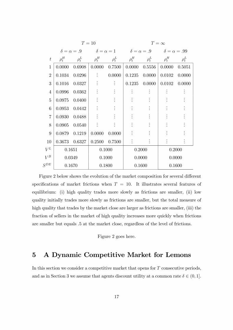
The examples in Table 1 illustrate our results for a market with uH = 1, cH = :6,
uL = :4, cL = :2, and qL = :2. It is easy to verify that frictions are small (i.e.,
both SF:1 and SF:2 hold) for these examples, although the su¢ cient condition in
Proposition 2 for uniqueness does not hold when � = � = :9. When the market is of
�nite duration (e.g., T = 10) buyers make low and negligible o¤ers at the market open,
4For example, there are DE similar to the one identi�ed in Proposition 5, except that there in
no trade in a single period.5In a market with stationary entry, Moreno and Wooders (2010)�s show that the surplus are com-
petitive as frictions vanish, but are above the competitive surplus when frictions are non-negligible.
In a continuous time version of the same model, Kim (2011) �nds the surplus to be competitive even
if frictions are non-negligible.
15

they make high and low price o¤ers at the market close, and they primarily make
negligible price o¤ers at intermediate dates. As frictions vanish, the market freezes
at intermediate dates as all price o¤ers are negligible. The surplus realized with
decentralized trading exceeds the static competitive surplus (of qL(uL � cL) = :16 ),and it is does so even in the limit as frictions vanish. Even as frictions vanish, not all
units trade.
In contrast, when the market is open inde�nitely, then decentralized trading yields
exactly the competitive surplus independently of the magnitude of frictions, so long
as they are small. At the market open, only low and negligible price o¤ers are made;
at every subsequent date only high and negligible price o¤ers are made, although
most o¤ers are negligible. As � approaches one, the probability of a high price o¤er
approaches zero (the market freezes). However, so long as � is less then one, the
probability of trading at each date is positive and constant, and thus all units trade
eventually.6
6When T =1 and � approaches one, then the expected delay for a high quality seller before he
trades approaches in�nity. Nonetheless, the gains to trade realized by trading high quality units is
asymptotically positive since the players are becoming perfectly patient.
16
T = 10 T =1� = � = :9 � = � = 1 � = � = :9 � = � = :99
t �Ht �Lt �Ht �Lt �Ht �Lt �Ht �Lt
1 0.0000 0.6908 0.0000 0.7500 0.0000 0.5556 0.0000 0.5051
2 0.1034 0.0296... 0.0000 0.1235 0.0000 0.0102 0.0000
3 0.1016 0.0327...
... 0.1235 0.0000 0.0102 0.0000
4 0.0996 0.0362...
......
......
...
5 0.0975 0.0400...
......
......
...
6 0.0953 0.0442...
......
......
...
7 0.0930 0.0488...
......
......
...
8 0.0905 0.0540...
......
......
...
9 0.0879 0.1219 0.0000 0.0000...
......
...
10 0.3673 0.6327 0.2500 0.7500...
......
...
V L 0.1651 0.1000 0.2000 0.2000
V B 0.0349 0.1000 0.0000 0.0000
SDE 0.1670 0.1800 0.1600 0.1600
Figure 2 below shows the evolution of the market composition for several di¤erent
speci�cations of market frictions when T = 10. It illustrates several features of
equilibrium: (i) high quality trades more slowly as frictions are smaller, (ii) low
quality initially trades more slowly as frictions are smaller, but the total measure of
high quality that trades by the market close are larger as frictions are smaller, (iii) the
fraction of sellers in the market of high quality increases more quickly when frictions
are smaller but equals .5 at the market close, regardless of the level of frictions.
Figure 2 goes here.
5 A Dynamic Competitive Market for Lemons
In this section we consider a competitive market that opens for T consecutive periods,
and as in Section 3 we assume that agents discount utility at a common rate � 2 (0; 1].
17

The supply and demand schedules are de�ned as follows. Let p = (p1; :::; pT ) 2 RT+be a sequence of prices. The gains to trade to sellers of quality � 2 fH;Lg is
v� (p) = maxt2f1;:::;Tg
f0; �t�1(pt � c� )g;
where �t�1(pt � c� ) is the gain to trade to a � -quality seller who supplies at t; andzero is the utility of not trading. The supply of � -quality good, S� (p); is the set of
sequences s� = (s�1; :::; s�T ) 2 RT+ satisfying:
(S:1)XT
t=1s�t � q� ,
(S:2) s�t > 0 implies �t�1(pt � c� ) = v� (p), and
(S:3)�XT
t=1s�t � q�
�v� (p) = 0.
Condition S:1 requires that no more of good � than is available, q� , is supplied.
Condition S:2 requires that supply is positive only in periods where it is optimal to
supply. Condition S:3 requires that supply be equal to the total amount available,
q� ; if the gain to trade for a � -quality seller is positive (i.e., when v� (p) > 0).
Denote by ut 2 [uL; uH ] the expected value to buyers of a unit drawn at randomfrom those supplied at date t. If u = (u1; :::; uT ) is a sequence of buyers�expected
values, then the gains to trade to a buyer is
vB(p; u) = maxt2f1;:::;Tg
f0; �t�1(ut � pt)g;
where �t�1(ut � pt) is the gain to trade to a buyer who demands a unit of the goodat t, and zero is the utility to not trading. The market demand, D(p; u), is the set of
sequences d = (d1; :::; dT ) 2 RT+ satisfying:
(D:1)XT
t=1dt � 1,
(D:2) dt > 0 implies �t�1(ut � pt) = vB(p; u), and
(D:3)�XT
t=1dt � 1
�vB(p; u) = 0.
ConditionD:1 requires that the total demand of good does not exceed the measure
of buyers, which we normalized to one. Condition D:2 requires that demand be
positive only at dates where buying is optimal. Condition D:3 requires that demand
be equal to the measure of buyers when buyers have positive gains to trade (i.e., when
vB(p; u) > 0).
18

With this notation in hand we introduce a notion of dynamic competitive equi-
librium along the lines in the literature �see e.g., Wooders (1998), Janssen and Roy
(2004), and Moreno and Wooders (2001).
A dynamic competitive equilibrium (CE) is a pro�le (p; u; sH ; sL; d) such that sH 2SH(p); sL 2 SL(p), and d 2 D(p; u); and for each t 2 f1; :::; Tg:
(CE:1) sHt + sLt = dt; and
(CE:2) sHt + sLt = dt > 0 implies ut =
uHsHt + uLsLt
sHt + sLt
.
Condition CE:1 requires that the market clear at each date, and condition CE:2
requires that the expectations described by the vector u are correct whenever there is
trade. For a market that opens for a single date (i.e., if T = 1); our de�nition reduces
to Akerlof�s.
The surplus generated in a CE, (p; u; sH ; sL; d), may be calculated as
SCE =X
�2fH;Lg
TXt=1
s�t �t�1(u� � c� ): (3)
As our next proposition shows, there a CE where all low quality units trade at
date 1 at the price uL, and none of the high quality units trade. Every CE has these
properties if traders are su¢ ciently patient.
Proposition 6. There is a CE in which all low quality units trade immediately at
the price uL and none of the high quality units trade, e.g., (p; u; sH ; sL; d) given by
pt = ut = uL for all t, sL1 = d1 = qL, and sH1 = sHt = sLt = dt = 0 for t > 1 is a
CE. In these equilibria the traders�gains to trade to low quality sellers is uL� cL, thegains to trade to high quality sellers and buyers is zero, and the surplus is
SCE = qL(uL � cL) = �S:
Moreover, if �T�1(cH � cL) > uL � cL, then every CE has these properties.
The intuition for why high quality does not trade when traders are patient is clear:
If high quality were to trade at t � T , then pt must be at least cH . Hence the gainsto trade to low quality sellers is at least �T�1(cH � cL) > uL � cL > 0, and thereforeall low quality sellers trade at prices greater than uL. But at a price p 2 (uL; cH)
19
only low quality sellers supply, and therefore the demand is zero. Hence all trade
is at prices of at least cH . Since u(qH) < cH by assumption, and all low quality is
supplied, there must be a date at which there is trade and the expected utility of a
random unit supplied is below cH . This contradicts that there is demand at such a
date. Given that there is not trade of high quality, the low quality sellers are the
short side of the market and therefore capture the entire surplus, i.e., the price is uL.
Proposition 7 below establishes that if traders are su¢ ciently impatient, then
there are dynamic competitive equilibria where high quality trades. Thus, the market
eventually recovers from adverse selection, e.g., in long-lived competitive markets the
adverse selection problem is less severe.
Proposition 7. If �T�1�uH � cL
�� uL � cL, then there are CE in which all units
trade.
The inequality of Proposition 7 holds for any discount factor when the market
remains open for in�nitely many periods. In this case, there are dynamic competitive
equilibria where all qualities trade. Our constructions in the proof of Proposition
7 suggest the high quality may have to trade with an increasingly long delay as the
discount factor approaches one. Thus, the question arises whether the surplus realized
from trading high quality units is positive, and how large it is, as � approaches one.
Proposition 8 provides an answer to these questions.
Proposition 8. If T =1; then as � approaches one the maximum surplus that canbe realized in a CE, ~SCE; is at least the surplus that can be realized in a DE, and is
greater that the competitive surplus, i.e.,
~SCE � ~SDE > �S:
Even though high quality units trade with an increasingly long delay as � ap-
proaches one, there are competitive equilibria that realize a surplus above the static
competitive surplus �S. Interestingly, as frictions vanish a market that opens for an
in�nite number of periods has dynamic competitive equilibria that generate the same
surplus as that of a decentralized market that opens for �nitely many periods. In
contrast, the CE of a market that opens for �nitely many periods generates the static
competitive surplus for discount factors su¢ ciently close to one.
20

6 Discussion
As propositions 1 to 7 show, the performance of dynamic market for lemons di¤ers
depending on the horizon over which they remain open and on the market infrastruc-
ture. When friction are small, a decentralized market that operates over a �nite
horizon is able to recover partially from adverse selection: some high quality units
and most low quality units trade, and the surplus is above the static competitive sur-
plus. As friction vanish some high quality units continue to trade, and all low quality
units trade, although some of these units trade with delay. Interestingly, trade tends
to concentrate in the �rst and last date, and the traders payo¤s and surplus does not
depend on the market duration; i.e., the surplus and payo¤s are the same whether
the market opens for just two periods, or a large but �nite number of periods, as
in the intermediate periods buyers make negligible price o¤ers; the waiting time is
necessary for low quality sellers to have a reservation price su¢ ciently low.
Dynamic competitive (centralized) markets that open for a �nite number of peri-
ods do not perform well when frictions are small as in equilibrium only low quality
trades �the equilibrium outcomes of these markets are the same as those of a static
competitive market. Dynamic competitive markets that open for an in�nite num-
ber of periods, however, have more e¢ cient equilibria where all low quality units and
some high quality units trade, and the surplus is above the static competitive surplus.
It is remarkable that the surplus realized in the most e¢ cient dynamic compet-
itive equilibrium of a market that open for in�nitely many periods is the same as
that generated in a decentralized market that open for �nitely many periods. Thus,
as friction vanish (i.e., as � and � approach one) an in�nitely (�nitely) lived central-
ized markets generates the same surplus as a �nitely (in�nitely) lived decentralized
markets. Table 2 below summarizes these results.
~S ~SDE ~SCE
T <1�qL + qH (1� q̂)
�(uL � cL) qL(uL � cL)
T =1 qL(uL � cL)�qL + qH (1� q̂)
�(uL � cL)
Table 2: Surplus as friction vanish.
It is worth noting that neither a decentralized market, nor a dynamic competi-
tive market is able to yield the surplus that may be realized by a (static) e¢ cient
21
mechanism (i.e., a mechanism that maximizes the surplus over all incentive compat-
ible and individually rational mechanisms). In our context, a mechanism is de�ned
by a collection [(pH ; zH); (pL; zL)]; specifying for each quality report � 2 fH;Lg amoney transfer from the buyer to the seller, p� 2 R+; and a probability that theseller transfers the good to the buyer, z� 2 [0; 1].7
An e¢ cient mechanism is a solution to the problem
max(p;z)2R2+�[0;1]2
qHzH(uH � cH) + qLzL(uL � cL)
subject to
p� � z�c� � p� � z�c� for each � ; � 2 fH;Lg; (IC:�)
qHzHuH + qLzLuL � (qHpH + qLpL) � 0; (IR:B)
p� � z�c� � 0 for each � 2 fH;Lg: (IR:�)
The constraint IC:� guarantees that the mechanism is incentive compatible, i.e., it
is optimal for a type � seller to report his type truthfully. The constraints IR:B
and IR:� guarantee that participating in the mechanism is individually rational for
buyers and sellers; i.e., that no trader obtains a negative expected payo¤.
It is straightforward to show that the e¢ cient mechanism satis�es zL = 1 > zH =
qL(uL � cL)=�cH � cL � qH(uH � cL)
�; and generates a surplus of
S� = qL(uL � cL) + qH(uH � cH)cH � qHuH � (1� qH)cL q
L(uL � cL):
Obviously, S� > qL(uL � cL); since qHuH + (1� qH)cL < u(qH) < cH by assumption.By Proposition 2 the surplus in a decentralized market increases with � and �:
Hence using the limiting surplus provided in Proposition 3 we have
S� � SDE > S� � ~SDE
=qH(uH � cH)2(uL � cL)
(uH � cL) (cH � (1� qH)cL � qHuH)> 0:
7By the Revelation Principle, we can restrict attention to �direct�mechanisms. Also note that
there is no need for buyers to report to the mechanism since they have no private information.
22
Hence, a decentralized market is not able to generate the surplus of a static e¢ cient
mechanism.8
As for the relation between the surplus generated in a long lived competitive
market and that a the static e¢ cient mechanism, we have
S� � SCE > S� � ~SCE = S� � ~SDE > 0:
Figure 2 below provides graphs of the mappings S�; S and �S????
Discuss: For markets for lemons with stationary entry, Janssen and Roy (2002
and 2000?) ...have shown that the only stationary dynamic competitive equilibrium
is the repetition of the static competitive equilibrium.9 Thus, time alone does not
explain the di¤erence in surplus realized under centralized and decentralized trade.
Discuss: Camargo and Lester
7 Appendix: Proofs
We begin by establishing a number of lemmas.
Lemma 1. Assume that T > 1, and let (�; rH ; rL) be a DE. Then for each t 2f1; :::; Tg:
(L1:1) �t(maxfrHt ; rLt g) = 1:
(L1:2) q�t > 0 for � 2 fH;Lg:
(L1:3) rHt = cH > rLt ; V
Bt > 0 = V Ht , and V
Lt � �(cH � cL):
(L1:4) qHt+1 � qHt :
(L1:5) �t(cH) = 1:
(L1:6) �t(p) = �t(rLt ) for all p 2 [rLt ; cH):
(L1:7) �LT = 1:
8Gale (1996) studies the properties of the competitive equilibria of markets with adverse selection
where agents exchange contracts specifying a price and a probability of trade, and shows that even
with a complete contract structure, equilibria are not typically incentive-e¢ cient.9They also �nd non-stationary equilibria, however, where all qualities trade although with delay.
The authors do not evaluate the surplus realized at these equilibria �they focus on the issue of price
volatility.
23
(L1:8) If �Lt = �Ht ; then q
�t+1 = q
�t+1 for � 2 fH;Lg:
Proof: Let t 2 f1; :::; Tg.We prove L1:1: Write �p = maxfrHt ; rLt g, and suppose that �t(�p) < 1. Then there
is p̂ > �p in the support of �t: Since I(�p; r�t ) = I(p̂; r�t ) = 1 for � 2 fH;Lg, we have
V Bt � �X
�2fH;Lg
q�t I(�p; r�t )(u
� � p̂) +
241� � X�2fH;Lg
q�t I(�p; r�t )
35 �V Bt+1= �
X�2fH;Lg
q�t (u� � �p) + (1� �) �V Bt+1
> �X
�2fH;Lg
q�t (u� � p̂) + (1� �) �V Bt+1
= �X
�2fH;Lg
q�t I(p̂; r�t )(u
� � p̂) +
241� � X�2fH;Lg
q�t I(p̂; r�t )
35 �V Bt+1;which contradicts DE:B.
We prove L1:2 by induction: Let � 2 fH;Lg: We have q�1 = q� > 0: Assume thatq�k > 0 for some k � 1; q�k+1 > 0: Since � 2 (0; 1); we have (1� ���k)q�k > 0: Hence
q�k+1 =(1� ���k)q�kqLk + q
Lk
> 0:
We prove L1:3 by induction. Because V �T+1 = 0 for � 2 fB;H;Lg; then DE:Hand DE:L imply
rHT = cH + �V HT+1 = c
H > cL = rLT = cL + �V LT+1:
Hence �T (cH) = 1 by L1:1, and therefore V HT = 0 and V LT � �(cH � cL): Moreover,0 < qLT
�uL � cL
�� V BT : Assume that L1:3 holds for k � T ; we show that it holds for
k � 1: Since V Hk = 0; DE:H implies rHk�1 = cH + �V Hk = cH : Since V Lk = �(c
H � cL);then DE:L implies rLk�1 = c
L + �V Lk � (1 � ��)cL + ��cH < cH : Hence �k(cH) = 1by L1:1, and therefore V Hk�1 = 0 and V
Lk�1 � �(cH � cL). Also V Bk+1 � �V Bk > 0:
In order to prove L1:4; note that L1:2 implies �Ht � �Lt . Hence
qHt+1 =
�1� ��Ht
�qHt�
1� ��Ht�qHt +
�1� ��Lt
�qLt� qHt :
As for L1:5; it is a direct implication of L1:1 and L1:2:
24
We prove L1:6: Suppose that �t(p) > �t(rLt ) for some p 2 (rLt ; rHt ): Then there isp̂ in the support of �t such that rLt < p̂ < r
Ht : Since I(p̂; r
Lt ) = 1 and I(p̂; r
Ht ) = 0; we
have
V Bt � �X
�2fH;Lg
q�t I(rLt ; r
�t )(u
� � rLt ) +
241� � X�2fH;Lg
q�t I(rLt ; r
�t )
35 �V Bt+1= �qLt
�uL � rLt
�+�1� �qLt
��V Bt+1
> �qLt�uL � p̂
�+�1� �qLt
��V Bt+1
= �X
�2fH;Lg
q�t I(p̂; r�t )(u
� � p̂) +
241� � X�2fH;Lg
q�t I(p̂; r�t )
35 �V Bt+1;which contradicts DE:B.
We prove �LT = 1: Suppose by way of contradiction that �LT < 1: Then there is
p̂ < cL in the support of �T : Since I(p̂; rHt ) = 0; and VBT+1 = 0; we have VT (p̂) = 0:
However, VT (cL) = qLT�uL � cL
�> 0 by L1:3; which contradicts DE:B.
We prove L1:8: We have Hence �Lt = �Ht implies
q�t+1 =(1� ���t ) q�t�
1� ��Ht�qHt +
�1� ��Lt
�qLt=
q�tqHt + q
Lt
= q�t . �
Proof of Proposition 1. Follows from lemmas L1:3; L1:5 and L1:6 above. �
As argued above, L1:5 and L1:6 imply that in a market equilibrium the only
price o¤ers that may be made with positive probability each date t are cH ; rLt ; and
prices below rLt : Therefore the distribution of transaction prices is determined by the
probabilities of o¤ering these prices, given by �Ht = �Ht , �
Lt = �
Lt ��Ht ; and 1��Ht ��Lt ;
respectively. Lemma 2 establishes some properties that these probabilities have in a
DE.
Lemma 2. Assume that T > 1, and let (�H ; �L; rH ; rL) be a DE. Then:
(L2:1) �HT + �LT = 1.
(L2:2) �Ht + �Lt > 0 for each t 2 f1; :::; Tg.
(L2:3) �H1 = 0 < �L1 :
Proof: Since �HT + �LT = �
LT ; then L2:1 follows from L1:7:
25
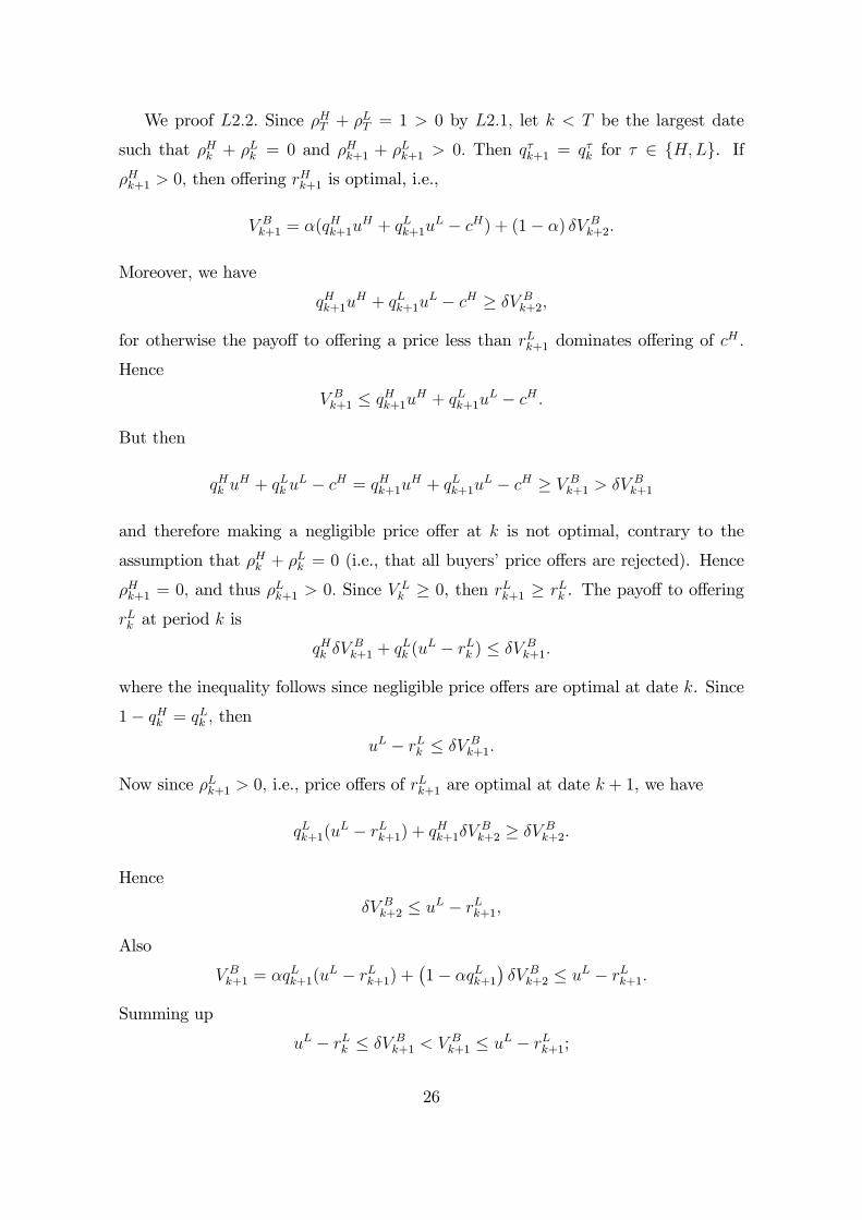
We proof L2:2: Since �HT + �LT = 1 > 0 by L2:1; let k < T be the largest date
such that �Hk + �Lk = 0 and �Hk+1 + �
Lk+1 > 0: Then q�k+1 = q�k for � 2 fH;Lg. If
�Hk+1 > 0; then o¤ering rHk+1 is optimal, i.e.,
V Bk+1 = �(qHk+1u
H + qLk+1uL � cH) + (1� �) �V Bk+2:
Moreover, we have
qHk+1uH + qLk+1u
L � cH � �V Bk+2;
for otherwise the payo¤ to o¤ering a price less than rLk+1 dominates o¤ering of cH :
Hence
V Bk+1 � qHk+1uH + qLk+1uL � cH :
But then
qHk uH + qLk u
L � cH = qHk+1uH + qLk+1uL � cH � V Bk+1 > �V Bk+1
and therefore making a negligible price o¤er at k is not optimal, contrary to the
assumption that �Hk + �Lk = 0 (i.e., that all buyers�price o¤ers are rejected). Hence
�Hk+1 = 0; and thus �Lk+1 > 0: Since V
Lk � 0, then rLk+1 � rLk . The payo¤ to o¤ering
rLk at period k is
qHk �VBk+1 + q
Lk (u
L � rLk ) � �V Bk+1:
where the inequality follows since negligible price o¤ers are optimal at date k. Since
1� qHk = qLk ; thenuL � rLk � �V Bk+1:
Now since �Lk+1 > 0; i.e., price o¤ers of rLk+1 are optimal at date k + 1, we have
qLk+1(uL � rLk+1) + qHk+1�V Bk+2 � �V Bk+2:
Hence
�V Bk+2 � uL � rLk+1;
Also
V Bk+1 = �qLk+1(u
L � rLk+1) +�1� �qLk+1
��V Bk+2 � uL � rLk+1:
Summing up
uL � rLk � �V Bk+1 < V Bk+1 � uL � rLk+1;
26
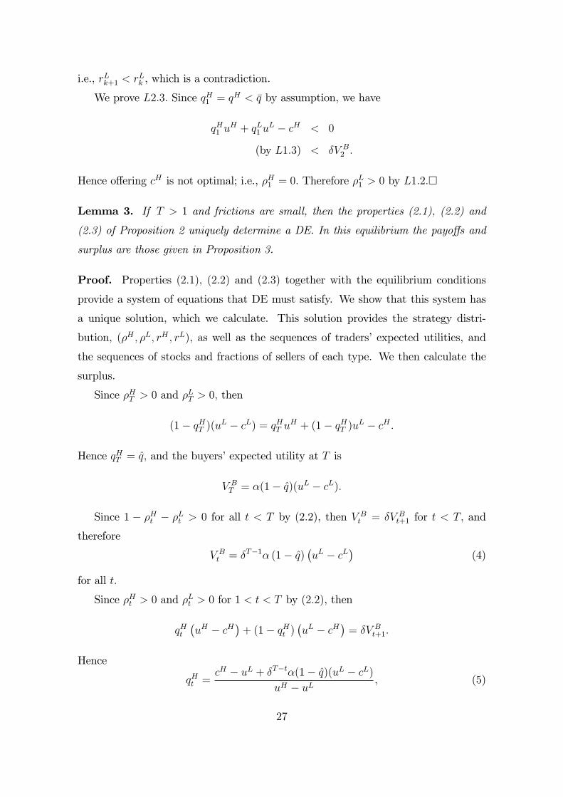
i.e., rLk+1 < rLk , which is a contradiction.
We prove L2:3: Since qH1 = qH < �q by assumption, we have
qH1 uH + qL1 u
L � cH < 0
(by L1:3) < �V B2 :
Hence o¤ering cH is not optimal; i.e., �H1 = 0: Therefore �L1 > 0 by L1:2:�
Lemma 3. If T > 1 and frictions are small, then the properties (2.1), (2.2) and
(2.3) of Proposition 2 uniquely determine a DE. In this equilibrium the payo¤s and
surplus are those given in Proposition 3.
Proof. Properties (2:1); (2:2) and (2:3) together with the equilibrium conditions
provide a system of equations that DE must satisfy. We show that this system has
a unique solution, which we calculate. This solution provides the strategy distri-
bution, (�H ; �L; rH ; rL), as well as the sequences of traders�expected utilities, and
the sequences of stocks and fractions of sellers of each type. We then calculate the
surplus.
Since �HT > 0 and �LT > 0; then
(1� qHT )(uL � cL) = qHT uH + (1� qHT )uL � cH :
Hence qHT = q̂; and the buyers�expected utility at T is
V BT = �(1� q̂)(uL � cL):
Since 1 � �Ht � �Lt > 0 for all t < T by (2:2), then V Bt = �V Bt+1 for t < T; and
therefore
V Bt = �T�1� (1� q̂)�uL � cL
�(4)
for all t:
Since �Ht > 0 and �Lt > 0 for 1 < t < T by (2:2), then
qHt�uH � cH
�+ (1� qHt )
�uL � cH
�= �V Bt+1:
Hence
qHt =cH � uL + �T�t�(1� q̂)(uL � cL)
uH � uL ; (5)
27

for 1 < t < T; and qHT = q̂ by L4:3.
Since �Lt > 0 and 1� �Ht � �Lt > 0 for t < T by (2:2), then
�qLt�uL � rLt
�+ (1� �qLt )�V Bt+1 = �V Bt+1;
i.e.,
�V Bt+1 = uL � rLt :
Hence for t < T we have
rLt = uL � �T�t�(1� q̂)(uL � cL); (6)
and rLT = cL.
Since rLt � cL = �V Lt+1 for all t by DE:L; then
uL � cL � �T�t�(1� q̂)(uL � cL) = �V Lt+1:
Reindexing we get
V Lt =uL � cL�
� �T�t�(1� q̂)(uL � cL); (7)
for t > 1: And since �H1 = 0 by (2:1), then
V L1 = �VL2 =
�1� �T�1� (1� q̂)
� �uL � cL
�: (8)
Again since rLt � cL = �V Lt+1 for all t; then the expected utility of a low-quality
seller is
V Lt = ��Ht (c
H � cL) + (1� ��Ht )�V Lt+1;
i.e.,
V Lt � �V Lt+1 = ��Ht (cH � cL � �V Lt+1):
Using equation (7), then for 1 < t < T we have
V Lt � �V Lt+1 =�1� ��
��uL � cL
�:
Hence �1� ��
��uL � cL
�= ��Ht (c
H � cL � �V Lt+1):
Solving for �Ht yields
�Ht =1� ���
uL � cL
cH � uL + �T�t�(1� q̂)(uL � cL)(9)
28

for 1 < t < T: Recall that �H1 = 0: Clearly �Ht > 0: Further, since ���cH � uL
�>
uL � cL; then�Ht < (1� �)
uL � cL�� (cH � uL) < 1:
Since low �LT�1 > 0 and 1 � �LT�1 � �HT�1 > 0 by (2:2), then uL � rLT�1 = �V BT :
Hence
V LT = ��HT (c
H � cL);
implies
��(1� q̂)(uL � cL) = uL � cL � ���HT (cH � cL).
Solving for �HT yields
�HT =uL � cL � ��(1� q̂)(uL � cL)
�� (cH � cL) = (1� ��(1� q̂)) (uL � cL)�� (cH � cL) : (10)
Since 0 < 1� �� (1� q̂) < 1; and ���cH � cL
�> (uL � cL), then 0 < �HT < 1:
Finally, we compute �Lt : For each t 2 f1; : : : ; T � 1g, we have
qHt+1 =(1� ��Ht )qHt
(1� ��Ht )qHt + (1� �(�Lt + �Ht ))qLt:
Solving for �Lt we obtain
�Lt = (1� ��Ht )qHt+1 � qHt
�qHt+1 (1� qHt )(11)
for t < T: Since 1 � qHt+1 � qHt and �Ht < 1; then �Lt > 0: And since �
�cH � uL
�>
���cH � uL
�> uL � cL, then
uL � cLcH � uL < � < 1;
and
(1� �) uL � cLcH � uL < 1:
Using (5), for t > 1 we have
qHt+1 � qHt�qHt+1 (1� qHt )
=(1� �)�T�t�1(1� q̂)(uL � cL)
cH � uL + �T�t�1�(1� q̂)(uL � cL)
�uH � uL
uH � cH � �T�t�(1� q̂)(uL � cL)
�< (1� �)(1� q̂)(u
L � cL)cH � uL
�uH � uL
uH � cH � (1� q̂)(uL � cL)
�= (1� �) u
L � cLcH � uL
< 1:
29
Hence �Lt < 1: Since
��1� qH
�> 1�
�1� (1� q̂) uL � cL
� (cH � uL)
�qH
q̂> 1� q
H
q̂
by SF:2; using (5) again and noticing that �H1 = 0; and qH2 � q̂ as shown above we
have
�L1 =qH2 � qH
qH2 � (1� qH)<
qH2 � qH
qH2
�1� qH
q̂
� = qH2 � qH
qH2 � qHqH2q̂
< 1:
Finally, �LT + �HT = 1 implies
�LT = 1� �HT = 1�uL � cL
�� (cH � uL) (1� ��(1� q̂)) : (12)
Since 0 < �HT < 1 as shown above, we have 0 < �LT < 1.
Using equations (4) and (8), noticing that qH + qL = 1; we can calculate the
surplus as
S =�qL + �T�1�qH (1� q̂)
� �uL � cL
�: � (13)
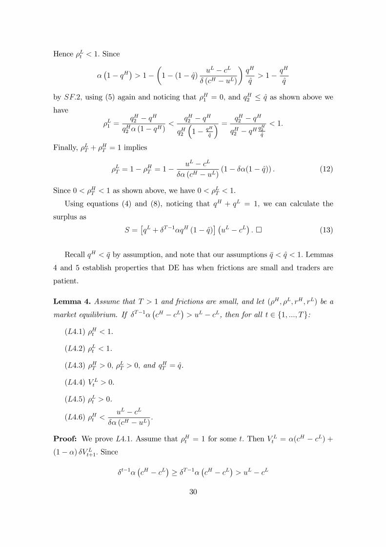
Recall qH < �q by assumption, and note that our assumptions �q < q̂ < 1: Lemmas
4 and 5 establish properties that DE has when frictions are small and traders are
patient.
Lemma 4. Assume that T > 1 and frictions are small, and let (�H ; �L; rH ; rL) be a
market equilibrium. If �T�1��cH � cL
�> uL � cL, then for all t 2 f1; :::; Tg:
(L4:1) �Ht < 1.
(L4:2) �Lt < 1.
(L4:3) �HT > 0; �LT > 0; and q
HT = q̂.
(L4:4) V Lt > 0.
(L4:5) �Lt > 0.
(L4:6) �Ht <uL � cL
�� (cH � uL) :
Proof: We prove L4:1: Assume that �Ht = 1 for some t: Then VLt = �(cH � cL) +
(1� �) �V Lt+1: Since
�t�1��cH � cL
�� �T�1�
�cH � cL
�> uL � cL
30
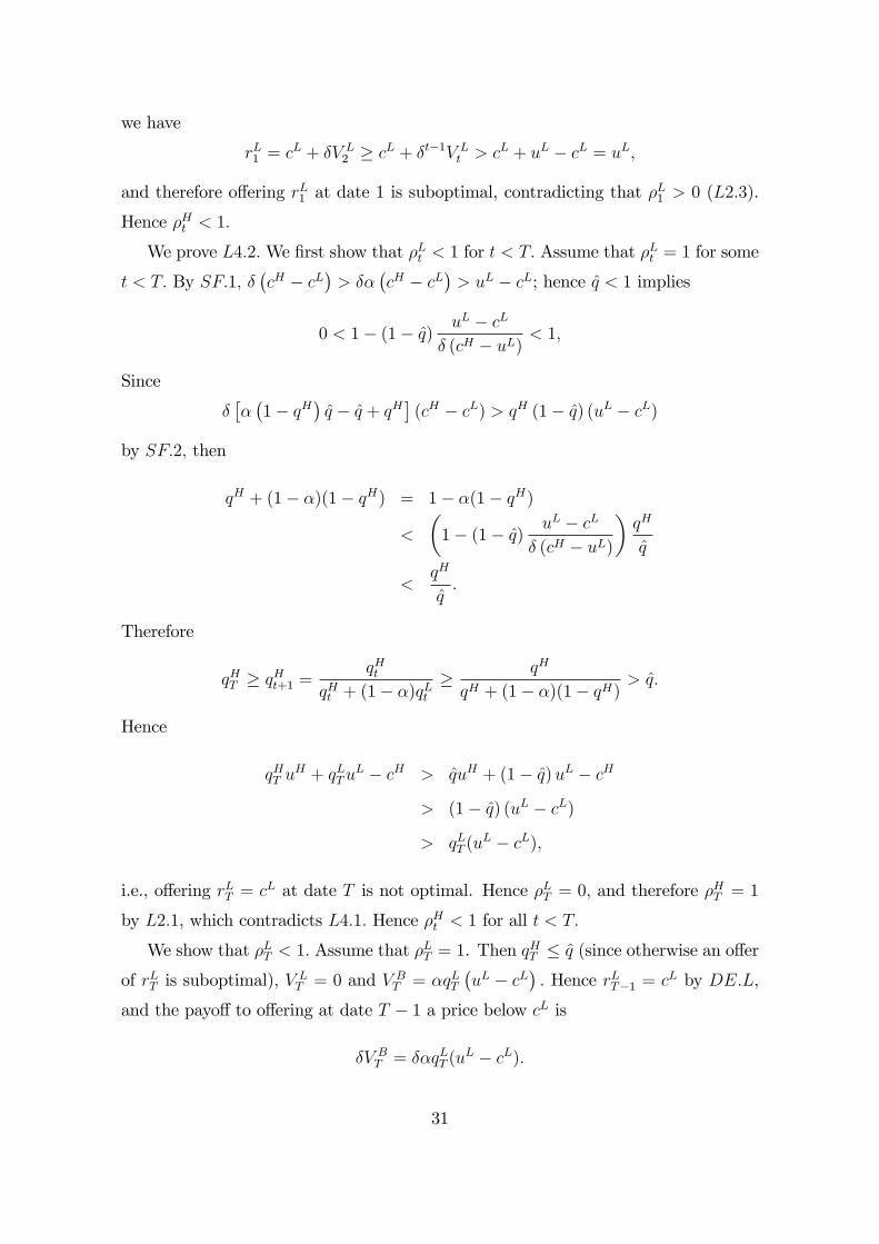
we have
rL1 = cL + �V L2 � cL + �t�1V Lt > cL + uL � cL = uL;
and therefore o¤ering rL1 at date 1 is suboptimal, contradicting that �L1 > 0 (L2:3).
Hence �Ht < 1:
We prove L4:2:We �rst show that �Lt < 1 for t < T: Assume that �Lt = 1 for some
t < T: By SF:1; ��cH � cL
�> ��
�cH � cL
�> uL � cL; hence q̂ < 1 implies
0 < 1� (1� q̂) uL � cL� (cH � uL) < 1;
Since
����1� qH
�q̂ � q̂ + qH
�(cH � cL) > qH (1� q̂) (uL � cL)
by SF:2; then
qH + (1� �)(1� qH) = 1� �(1� qH)
<
�1� (1� q̂) uL � cL
� (cH � uL)
�qH
q̂
<qH
q̂:
Therefore
qHT � qHt+1 =qHt
qHt + (1� �)qLt� qH
qH + (1� �)(1� qH) > q̂:
Hence
qHT uH + qLTu
L � cH > q̂uH + (1� q̂)uL � cH
> (1� q̂) (uL � cL)
> qLT (uL � cL);
i.e., o¤ering rLT = cL at date T is not optimal. Hence �LT = 0; and therefore �
HT = 1
by L2:1, which contradicts L4:1: Hence �Ht < 1 for all t < T:
We show that �LT < 1: Assume that �LT = 1. Then q
HT � q̂ (since otherwise an o¤er
of rLT is suboptimal); VLT = 0 and V BT = �qLT
�uL � cL
�: Hence rLT�1 = c
L by DE:L,
and the payo¤ to o¤ering at date T � 1 a price below cL is
�V BT = ��qLT (uL � cL):
31

Hence
qLT�1(uL � cL) + qHT�1�V BT � �V BT = qLT�1(u
L � cL)�1� ��qLT
�> 0;
i.e., the payo¤ to o¤ering cL at date T � 1 is greater than that of o¤ering less thancL. Therefore �LT�1+ �
HT�1 = 1. Since q
HT�1 � qHT by L1:4 and qHT � q̂; then the payo¤
to o¤ering cH at T � 1 is
qHT�1uH + qLT�1u
L � cH � qHT uH + qLTu
L � cH
� qLT (uL � cL)
� qLT�1(uL � cL)
< qLT�1(uL � cL) + qHT�1�V BT ;
where the last term is the payo¤to o¤ering cL at T�1. Hence �HT�1 = 0; and therefore�LT�1 = 1, which contradicts that �
LT�1 < 1 as shown above. Hence �
LT < 1.
We prove L4:3:We have �HT < 1 by L4:1; and therefore L2:1 implies �LT > 0: Since
�LT < 1 by L4:2, then �HT > 0 by L2:1. Now, since both high price o¤ers and low price
o¤ers are optimal at date T; and reservation prices are rHT = cH and rLT = c
L; we have
qHT uH + qLTu
L � cH = qLT (uL � cL);
i.e.,
qHT uH + (1� qHT )uL � cH = (1� qHT )(uL � cL):
Hence
qHT =cH � cLuH � cL = q̂:
We prove L4:4 by induction. By L4:3; V LT = ��HT�cH � cL
�> 0: Assume that
V Lk+1 > 0 for some k � T: Since rLk � cL = �V Lk+1 by DE:L; then we have
V Lk = ���Hk�cH � cL
�+ �Lk
�rLk � cL
��+�1� �
��Hk + �
Lk
���V Lt+1
= ��Hk�cH � cL
�+�1� ��Hk
��V Lk+1
> 0:
We prove L4:5: Suppose by way of contradiction that �Lt = 0 for some t: Since
�LT > 0 by L4:3; then t < T: Also �Lt = 0 implies �
Ht > 0 by L2:2: Since �
Ht < 1 by
L4:1; then buyers are indi¤erent at date t between o¤ering cH or less than rLt , i.e.,
qHt uH + qLt u
L � cH = �V Bt+1 < V Bt+1:
32

We show that �Ht+1 = 0: Suppose that �Ht+1 > 0; then
V Bt+1 = ��qHt+1u
H + qLt+1uL � cH
�+ (1� �)�V Bt+2:
Hence
qHt uH + qLt u
L � cH < ��qHt+1u
H + qLt+1uL � cH
�+ (1� �)�V Bt+2;
But �Lt = 0 implies qHt+1 = q
Ht ; and therefore
qHt+1uH + qLt+1u
L � cH < �V Bt+2;
i.e., o¤ering cH yields a payo¤ smaller than o¤ering less than rLt+1; which contradicts
that �Ht+1 > 0:
Since �Ht+1 = 0; then DE:L implies
V Lt+1 = ��Lt+1�rLt+1 � cL
�+�1� ��Lt+1
��V Lt+2
= �V Lt+2;
and since V Lt+1 > 0 by L4:4; hence VLt+2 > 0; and therefore DE:L implies
rLt = cL + �V Lt+1 = c
L + �2V Lt+2 < cL + �V Lt+2 = r
Lt+1:
We show that these facts: �Ht+1 = 0 < �Lt+1 < 1 and rLt < rLt+1 are incompatible,
thereby proving that �Lt > 0:
The payo¤ to o¤ering rLt at period t is
qHt �VBt+1 + q
Lt (u
L � rLt ) � �V Bt+1;
where the inequality follows since negligible price o¤ers are optimal (because �Lt =
0 < �Ht < 1). Noticing that qHt = 1� qLt ; this inequality becomes
uL � rLt � �V Bt+1:
Since 0 < �Lt+1 < 1; i.e., price o¤ers of rLt+1 and of less than r
Lt+1 are optimal, we have
V Bt+1 = �qLt+1(u
L � rLt+1) +�1� �qLt+1
��V Bt+2 = �V
Bt+2:
Hence
V Bt+1 = uL � rLt+1:
33

Summing up
uL � rLt � �V Bt+1 < V Bt+1 = uL � rLt+1;
i.e., rLt � rLt+1, which contradicts rLt < rLt+1.We prove L4:6: Since V Lt � 0; and rLt � cL = �V Lt+1 by DE:L; we have
V Lt = ���Ht�cH � cL
�+ �Lt
�rLt � cL
��+�1� �
��Ht + �
Lt
���V Lt+1
� ��Ht�cH � cL
�:
Since �Lt > 0 by L4:5 (i.e., price o¤ers of rLt are optimal), and V
Bt > 0 by L1:2; then
uL > rLt : Hence
uL � cL > rLt � cL = �V Lt+1 � ���Ht�cH � cL
�;
i.e.,
�Ht <uL � cL
�� (cH � uL) : �
Lemma 5. Assume that T > 1 and frictions are small, and let (�H ; �L; rH ; rL) be a
market equilibrium. If �T�1��cH � cL
�> uL � cL, then �Ht+1 > 0 and �Lt + �Ht < 1
for all t 2 f1; :::; T � 1g.
Proof: Let t 2 f1; :::; T � 1g: We proceed by showing that (i) �Ht > 0 implies
�Lt + �Ht < 1, and that (ii) �Lt + �
Ht < 1 implies �Ht+1 > 0: Then Lemma 5 follows
by induction: Since �H1 = 0 by L2:3 and �L1 < 1 by L4:2; then �H1 + �L1 < 1; and
therefore �H2 > 0 by (ii). Assume that the claim holds for k 2 f1; :::; T � 1g; we showthat �Hk+1 + �
Lk+1 < 1 and �
Hk+2 > 0: Since �
Hk+1 > 0; then �
Hk+1 + �
Lk+1 < 1 by (i), and
therefore �Hk+2 > 0 by (ii).
We establish (i), i.e., �Ht > 0 implies �Lt + �
Ht < 1. Suppose not; let t < T be the
�rst date such that �Ht > 0 and �Lt + �
Ht = 1. Since �
Lt + �
Ht = 1 (i.e., all low quality
34
seller who are matched trade) and qHt � qH1 = qH by L1:4; then L4:6 implies
qHt+1 =
�1� ��Ht
�qHt
(1� ��Ht ) qHt + (1� �)qLt
>
�1� uL � cL
� (cH � uL)
�qHt�
1� uL � cL� (cH � uL)
�qHt + (1� �)qLt
>
�1� uL � cL
� (cH � uL)
�qH�
1� uL � cL� (cH � uL)
�qH + (1� �)(1� qH)
;
where the �rst and second inequality hold since qHt+1 is decreasing in �Ht and increasing
in qHt (and qH > qHt ). Since
����1� qH
�q̂ � q̂ + qH
�(cH � cL) > qH (1� q̂) (uL � cL)
by SF:2, then we have�1� uL � cL
� (cH � uL)
�qH + (1� �)(1� qH) = � uL � cL
� (cH � uL)qH + 1� �(1� qH)
< � uL � cL� (cH � uL)q
H + 1��1�
�1� (1� q̂) uL � cL
� (cH � uL)
�qH
q̂
�=
qH
q̂
�1� uL � cL
� (cH � uL)
�:
Hence
qHt+1 >
�1� uL � cL
� (cH � uL)
�qH�
1� uL � cL� (cH � uL)
�qH
q̂
= q̂ = qT ;
which contradicts L1:4:
Next we prove (ii), i.e., �Lt + �Ht < 1 implies �
Ht+1 > 0. Suppose not; let t < T be
such that �Lt + �Ht < 1 and �
Ht+1 = 0: Since �
Lt > 0 by L4:5, then o¤ers of r
Lt and of
less than rLt are optimal at date t, and we have
uL � rLt = �V Bt+1:
Since �Ht+1 = 0 we have
V Lt+1 = �VLt+2:
35
Therefore L4:4 implies
rLt+1 = cL + �V Lt+2 = c
L + V Lt+1 > cL + �V Lt+1 = r
Lt :
Since 0 < �Lt+1 < 1 by L4:2 and L4:5, then o¤ers of rLt+1 and of less than rLt+1 are
optimal at t+ 1; i.e.,
uL � rLt+1 = �V Bt+2;
and
V Bt+1 = �VBt+2:
Summing up
uL � rLt = �V Bt+1 < V Bt+1 = �V Bt+2 = uL � rLt+1;
i.e.,
rLt > rLt+1;
which is a contradiction. �
Proof of propositions 2 and 3. (2:1) follows from L2:3 and L4:2: (2:2) follows
from L4:5 and Lemma 5. (2:3) follows from L2:1 and L4:3:???
Proof of Proposition 4. We have ~�H1 = lim�;�!1 �H1 = 0; and for 1 < t < T; using
(9) above we have
~�Ht = lim�;�!1
�Ht = lim�;�!1
1� ���
uL � cL
cH � uL + �T�t�(1� q̂)(uL � cL)= 0:
Also (10) yields
~�HT = lim�;�!1
�HT =uL � cLcH � uL q̂:
Since
lim�;�!1
qHt = lim�;�!1
cH � uL + �T�t�(1� q̂)(uL � cL)uH � uL = q̂;
for t > 1; then (11) yields
~�Lt = lim�;�!1
�Lt = lim�;�!1
(1� ��Ht )qHt+1 � qHt
�qHt+1 (1� qHt )= 0:
for 1 < t < T: Also
~�L1 = lim�;�!1
�L1 =q̂ � qHq̂ � q̂qH :
36
And (12) yields
~�LT = lim�;�!1
�LT = 1�uL � cLcH � uL q̂:
Note that the limiting values (~�H ; ~�L) form a sequence probability distributions, i.e.,
~�Ht ; ~�Lt < 0 and ~�
Ht + ~�
Lt < 1 for all t 2 f1; :::; Tg. (However, one can show that for
� = � = 1 there are multiple decentralized market equilibria.)
As for traders�expected utilities, (4) implies
~V Bt = lim�;�!1
�T�t� (1� q̂)�uL � cL
�= (1� q̂)
�uL � cL
�;
(7) implies
~V L1 = lim�;�!1
�1� �T�1� (1� q̂)
� �uL � cL
�= q̂
�uL � cL
�;
and ~V Ht = lim�;�!1 VHt = 0:
Finally, using (13) we get
S = lim�;�!1
�qL(uL � cL) + qH�T�1�(1� q̂)(uL � cL)
�=�qL + qH (1� q̂)
�(uL � cL): �
Proof of Proposition 5. Assume that T = 1; and frictions are small. We showthat the strategy distribution (�H ; �L; rH ; rL) given by rHt = cH , rLt = uL for all t;
�H1 = 0;
�L1 =�q � qH
� (1� qH) �q ;
and �Lt = 0;
�Ht =1� ���
uL � cLcH � uL
for t > 1 forms a decentralized market equilibrium.
Since q̂ > �q; SF:2 implies
��1� qH
�> 1�
�1� (1� q̂) uL � cL
� (cH � uL)
�qH
q̂
> 1� qH
q̂
> 1� qH
�q:
Then 0 < �L1 < 1: As ���cH � uL
�> uL � cL by SF:1; we have 0 < �Ht < 1 for all
t > 1 �recall that � < 1 by assumption. Since rHt = cH , rLt = u
L; then the expected
37

utilities buyers and high quality sellers are V Bt = V Ht = 0: For t > 1 low quality
sellers expected utility is V Lt = (uL � cL)=� . Then rHt = cH and rLt = uL satisfy
DE:H and DE:L; respectively. Using �H1 and �L1 we have
qH2 =qH
qH + (1� ��L1 )(1� qH)= �q:
And since �Lt = 0 for t > 1; then qHt = q
H1 = �q: Hence
qHt�uH � cH
�+ (1� qHt )
�uL � cH
�= 0:
Since rLt = uL; then the payo¤ to a low price o¤er is also zero. Then high, low and
negligible price o¤ers are optimal at date t > 1. Moreover, since V Bt = 0; then low
and negligible price o¤ers are optimal and date 1: Hence any distribution of price
o¤ers � such that �Ht and �Lt have the values de�ned above satis�es DE:B: Therefore
the strategy distribution de�ned is a decentralized market equilibrium. �
In lemmas 5 and 6 we establish some basic properties of dynamic competitive
equilibria.
Lemma 6. In every CE, (p; u; sH ; sL; d), we haveXftjsHt >0g
sLt < qL:
Proof. Let (p; u; sH ; sL; d) be a CE. For all t such that sHt > 0 we have
�t�1(pt � cH) = vH(p) � 0
by (S:2). Hence pt � cH : Also dt > 0 by CE:1; and therefore
vB(p) = �t�1(ut � pt) � 0
implies
0 � ut � pt � ut � cH ;
i.e., ut � cH = u(�q): ThussHt
sHt + sLt
� �q:
38
Hence
(1� �q)X
ftjsHt >0g
sHt � �qX
ftjsHt >0g
sLt :
Since XftjsHt >0g
sHt � qH < �q;
then
(1� �q)qH � (1� �q)X
ftjsHt >0g
sHt � �qX
ftjsHt >0g
sLt � qHX
ftjsHt >0g
sLt ;
i.e., XftjsHt >0g
sLt � 1� �q < 1� qH = qL: �
Lemma 7. Let (p; u;mH ;mL;mB) be a CE. If sH�t > 0 for some �t, then there is t < �t
such that sLt > 0 = sHt ; and
�t�1(uL � cL) � ��t�1(cH � cL):
Proof. Let (p; u; sH ; sL; d) be a CE, and assume that sH�t > 0: Then ��t�1(p�t�cH) =
vH(p) � 0 by S:2; and therefore p�t � cH :Hence vL(p) � ��t�1(p�t�cL) � �
�t�1(cH�cL) >0, and therefore
TXt=1
sLt = qL
by (S:3). SinceP
ftjsHt >0gsLt < q
L by Lemma 6, there there is t̂ such that sLt̂> 0 = sHt :
Hence dt̂ > 0 by CE:1 implies ut̂ = uL by CE:2; and pt̂ � uL by D:2. Also sLt̂ > 0
implies vL(p) = �t̂�1(pt̂ � cL) � ��t�1(p�t � cL) by S:2. Thus
�t̂�1(uL � cL) � �t̂�1(pt̂ � cL) � ��t�1(p�t � cL) � �
�t�1(cH � cL):
Since uL < cH this inequality implies t̂ < �t: �
Proof of Proposition 6. Let (p; u; sH ; sL; d) be a CE, and assume that �T�1(uH�cL) > uL � cL:
39
We show that sHt = 0 for all t 2 f1; : : : ; Tg. Suppose that sHt > 0 for some t.
Then Lemma 7 implies that there is t0 < t such that
uL � cL � �t0�1(uL � cL) � �t�1(cH � cL) � �T�1(cH � cL);
which is a contradiction.
We show that pt � uL for all t. If pt < uL for some t, then
vB(p; u) = maxt2f1;:::;Tg
(0; �t�1(ut � pt)) > 0;
and thereforePT
t=1 dt = 1. Since sHt = 0 for all t, then CE:1 implies
qL =TXt=1
sLt =
TXt=1
(sHt + sLt ) =
TXt=1
dt = 1;
which contradicts qL = 1� qH < 1. Hence pt � uL for all t.We now show that p1 = uL and sL1 = d1 = qL. Suppose sLt > 0. Then sHt = 0
implies ut = uL. By CE:1 we have dt > 0 and thus
�t�1(ut � pt) = �t�1(uL � pt) � 0
by D:2. This inequality, and pt � uL for all t, imply that pt = uL. If t > 1, then
p1 � uL implies p1� cL > �t�1(pt� cL), which contracts S:2. Hence sLt = 0 for t > 1.Since p1 � cL > 0, then vL(p) > 0 and thus
PTt=1 s
Lt � qL = 0 by S:3, which implies
that sL1 = qL. CE:1 and sH1 = 0 then implies d1 = q
L. �
Proof of Proposition 7. Assume that �T�1�uH � cL
�<�uL � cL
�: We show that
the pro�le (p; u; sH ; sL; d) given by pt = ut = uL for t < T; and pT = uT = uH ;
sH1 = 0; sL1 = q
L = d1; sLt = s
Ht = dt = 0 for 1 < t < T; s
HT = dT = q
H ; sLT = 0 is a
CE.
For high quality sellers we have vH(p) = �T�1(pT � cH) = �T�1(uH � cH) >0 > �t�1(pt � cH) for t < T; and hence SH(p) = f(0; :::; 0; qH)g: For low quality
sellers we have vL(p) = p1 � cL = uL � cL > �t�1(pt � cH) for t > 1: (In particular,uL�cL > �T�1(pT�cH) = �T�1(uH�cH).) Hence SH(p) = f(qL; 0; :::; 0)g: For buyers,vB(p; u) = 0 = �t�1(ut � pt) for all t: Hence D(p; u) = fd 2 RT+ j
PTt=1 dt � 1g; and
(qL; 0; :::; 0; qH) 2 D(p; u): Finally, note that buyers�value expectations at dates 1and T; u1 and uT ; are correct. Thus, the pro�le de�ned is a CE.
40

Assume that �T�1�uH � cL
���uL � cL
�:We show that the pro�le (p; u; sH ; sL; d)
given by pt = ut = uL for t < T;and pT = uT = �1�T�uL � cL
�+ cL; sH1 = 0;
sL1 = qL � q = d1; sLt = sHt = dt = 0 for 1 < t < T; and sHT = qH ; sLT = q; and
dT = q + qH ; where
q =
��uL � cL
�� �T�1(uH � cL)
�qH�
�T�1 (uL � cL)� (uL � cL)� ;
is a CE. Note that since qH < �q (i.e. u(qH) = qHuH + (1 � qH)uL < cH), and
uL � cL � �T�1�cH � cL
�� 0 by assumption, then
1� qH ���uL � cL
�� �T�1(uH � cL)
�qH�
�T�1 (uL � cL)� (uL � cL)�
=(uL � cL)� �T�1
�qHuH + (1� qH)uL � cL
���T�1 � 1
�(cL � uL)
>(uL � cL)� �T�1
�cH � cL
���T�1 � 1
�(cL � uL)
� 0;
and therefore q < qL:
For high quality sellers we have
vH(p) = �T�1(pT � cH)
= �T�1(�1�T�uL � cL
���cH � cL
�)
=�uL � cL
�� �T�1
�cH � cL
�)
> 0
> �t�1(pt � cH)
for all t < T: Hence SH(p) = f(0; :::; 0; qH)g: For low quality sellers we have
vL(p) = p1 � cL
= uL � cL
= �T�1(�1�T�uL � cL
�+ cL � cL)
= �T�1(pT � cL)
> �t�1(pt � cH)
> 0:
41
for all 1 < t < T: Hence SH(p) = f(sL1 ; 0; :::; sLT ) j sL1 + sLT = qLg: For buyers,vB(p; u) = 0 = �t�1(ut � pt) for all t: Hence D(p; u) = fd 2 RT+ j
PTt=1 dt � 1g;
and (qL; 0; :::; 0; qH) 2 D(p; u): Finally, we show that buyers value expectations arecorrect at dates 1 and T . Clearly u1 = uL is the correct expectation as only low
sellers supply at date 1. As for uT we have
ut =sHT
sHT + sLT
uH +sLT
sHT + sLT
uL
=qH
qH + quH +
q
qH + quL
= �1�T�uL � cL
�+ cL�1: �
Proof of Proposition 8. Assume that T =1: Consider the pro�le (p; u; sH ; sL; d)given by pt = ut = uL for t < �T ; and pt = ut = uH for t > �T , sH1 = 0; s
L1 = d1 = q
L;
sH�T = d �T = qH ; sL�T = 0; and s
Ht = s
Lt = dt = 0 for t =2 f1; �Tg; where �T is the unique
date satisfying
��T�2 �uH � cL� > uL � cL � � �T�1 �uH � cL�
By following the steps of the �st part of the proof of Proposition 7, it is easy to
see that this pro�le is a CE. The surplus is readily calculated as
SCE =X
�2fH;Lg
TXt=1
s�t �t�1(u� � c� ) = qL(uL � cL) + qH� �T�1(uH � cH):
We show that the surplus in this equilibrium approaches the surplus generated in a
decentralized market equilibrium with �nite T as friction vanish, ~SDE; we establishes
the proposition. In order to calculate the surplus as � approaches, note that
��T�2 >
uL � cLuH � cL � �
�T�1
i.e.,
1
ln �ln
�uL � cLuH � cL
�+ 1 � �T <
1
ln �ln
�uL � cLuH � cL
�+ 2:
Since
lim�!1
��
1ln �
ln�uL�cLuH�cL
�+1
�= lim
�!1
��
1ln �
ln�uL�cLuH�cL
�+2
�=uL � cLuH � cL
42

then
lim�!1
��T�1 =
uL � cLuH � cL :
Substituting, we have
lim�!1
SCE = qL(uL � cL) + qH(uH � cH) uL � cLuH � cL
=�qL + qH(1� q̂)
�(uL � cL)
= ~SDE:
43

References
[1] Akerlof, G., The Market for �Lemons�: Quality Uncertainty and the Market
Mechanism, Quarterly Journal of Economics (1970) 84, 488-500.
[2] Binmore, K. and M. Herrero (1988), Matching and Bargaining in Dynamic Mar-
kets, Review of Economic Studies (1988) 55, 17-31.
[3] Bilancini, E., and L. Boncinelli, Dynamic adverse selection and the size of the
informed side of the market, manuscript (2011).
[4] Blouin, M. , Equilibrium in a Decentralized Market with Adverse Selection,
Economic Theory (2003) 22, 245-262.
[5] Blouin, M., and R. Serrano , A Decentralized Market with Common Values
Uncertainty: Non-Steady States,�Review of Economic Studies (2001) 68, 323-
346.
[6] Camargo, B., and B. Lester, Trading dynamics in decentralized markets with
adverse selection, manuscript (2011).
[7] Gale, D.,Limit Theorems for Markets with Sequential Bargaining, Journal of
Economic Theory (1987) 43, 20-54.
[8] Gale, D., Equilibria and Pareto Optima of Markets with Adverse Selection, Eco-
nomic Theory 7, (1996) 207-235.
[9] Jackson, M., and T. Palfrey, E¢ ciency and voluntary implementation in markets
with repeated pairwise bargaining,�Econometrica (1999) 66, 1353-1388.
[10] Janssen, M., and S. Roy, Dynamic Trading in a Durable Good Market with
Asymmetric information,� International Economic Theory (2002) 43, 257 -
282.
[11] Kim, K., Information about sellers� past behavior in the market for lemons,
manuscript. 2011.
[12] Moreno, D., and J. Wooders, Prices, Delay and the Dynamics of Trade, Journal
of Economic Theory (2002) 104, 304-339.
44

[13] Moreno, D., and J. Wooders, Decentralized trade mitigates the lemons problem,
International Economic Review (2010) 51: 383-399.
[14] Moreno, D., and J. Wooders, The E¢ ciency of Centralized and Decentralized
Markets for Lemons, University of Arizona Working Paper (2001), 01-03 �
http://econ.arizona.edu/docs/Working_Papers/Misc%20Years/quality_y2.pdf.
[15] Morris, S., and H.S. Shin, Contagious adverse selection, manuscript 2011.
[16] Osborne, M., and A. Rubinstein, Bargaining and Markets, Academic Press, New
York, 1990.
[17] Rubinstein, A., and A. Wolinsky, Equilibrium in a Market with Sequential Bar-
gaining,�Econometrica (1985) 53, 1133-1150.
[18] Rubinstein, A., and A. Wolinsky, Decentralized Trading, Strategic Behavior and
the Walrasian Outcome, Review of Economic Studies (1990) 57, 63-78.
[19] Serrano, R., and O. Yosha, Decentralized information and the walrasian outcome:
a pairwise meetings market with private values,�manuscript, 1996.
[20] Wilson, C., The Nature of Equilibrium in Markets with Adverse Selection, The
Bell Journal of Economics (1980) 11, 108-130.
[21] Wolinsky, A., Information Revelation in a Market with Pairwise Meetings,
Econometrica (1990) 58, 1-23.
[22] Wooders, J., Walrasian Equilibrium in Matching Models,�Mathematical Social
Sciences (1998) 35, 245-259.
45
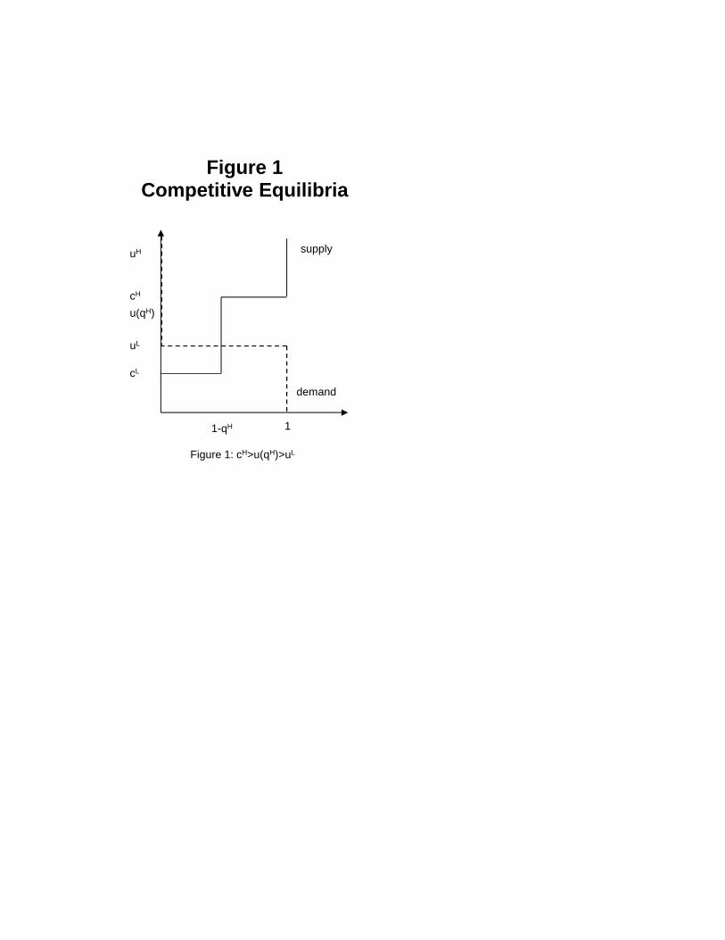
1
cL
uL
cH
uH
u(qH)
Figure 1: cH>u(qH)>uL
1-qH
supply
demand
Figure 1Competitive Equilibria

0.00
0.05
0.10
0.15
0.20
1 2 3 4 5 6 7 8 9 10 11
Figure 2(a): High Quality Stocks
d=a=.8
d=a=.9
d=a=1
0.00
0.10
0.20
0.30
0.40
0.50
0.60
0.70
0.80
1 2 3 4 5 6 7 8 9 10 11
Figure 2(b): Low Quality Stocks
d=a=.8
d=a=.9
d=a=1
0.00
0.10
0.20
0.30
0.40
0.50
0.60
0 1 2 3 4 5 6 7 8 9 10
Figure 2(c): Proportion of High Quality in the Market
d=a=.8
d=a=.9
d=a=1


