

ES159/259
Ch. 6 Single Variable Control

ES159/259
Single variable control
• How do we determine the motor/actuator inputs so as to command the end effector in a desired motion?
• In general, the input voltage/current does not create instantaneous motion to a desired configuration
– Due to dynamics (inertia, etc)– Nonlinear effects
• Backlash
• Friction
– Linear effects• Compliance
• Thus, we need three basic pieces of information:1. Desired joint trajectory
2. Description of the system (ODE = Ordinary Differential Equation)
3. Measurement of actual trajectory

ES159/259
SISO overview
• Typical single input, single output (SISO) system:
• We want the robot tracks the desired trajectory and rejects external disturbances
• We already have the desired trajectory, and we assume that we can measure the actual trajectories
• Thus the first thing we need is a system description
ES159/259
SISO overview
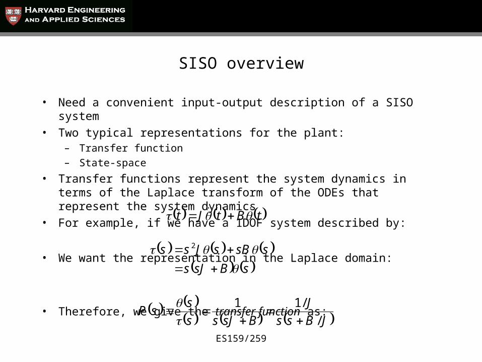
• Need a convenient input-output description of a SISO system
• Two typical representations for the plant:– Transfer function– State-space
• Transfer functions represent the system dynamics in terms of the Laplace transform of the ODEs that represent the system dynamics
• For example, if we have a 1DOF system described by:
• We want the representation in the Laplace domain:
• Therefore, we give the transfer function as:
tBtJt
sBsJs
ssBsJss
2
JBss
J
BsJss
ssP
/
/11

ES159/259
Review of the Laplace transform
• Laplace transform creates algebraic equations from differential equations
• The Laplace transform is defined as follows:
• For example, Laplace transform of a derivative:
– Integrating by parts:
0
dttxesx st
0
dtdt
tdxe
dt
tdxtx stLL
00
0
xssx
dttxestxedt
tdx stst
L

ES159/259
Review of the Laplace transform
• Similarly, Laplace transform of a second derivative:
• Thus, if we have a generic 2nd order system described by the following ODE:
• And we want to get a transfer function representation of the system, take the Laplace transform of both sides:
002
02
2
2
2
xsxsxsdtdt
txde
dt
txdtx st
LL
tFtkxtxbtxm
sFskxxssxbxsxsxsm
tFtxktxbtxm
0002
LLLL
ES159/259
Review of the Laplace transform
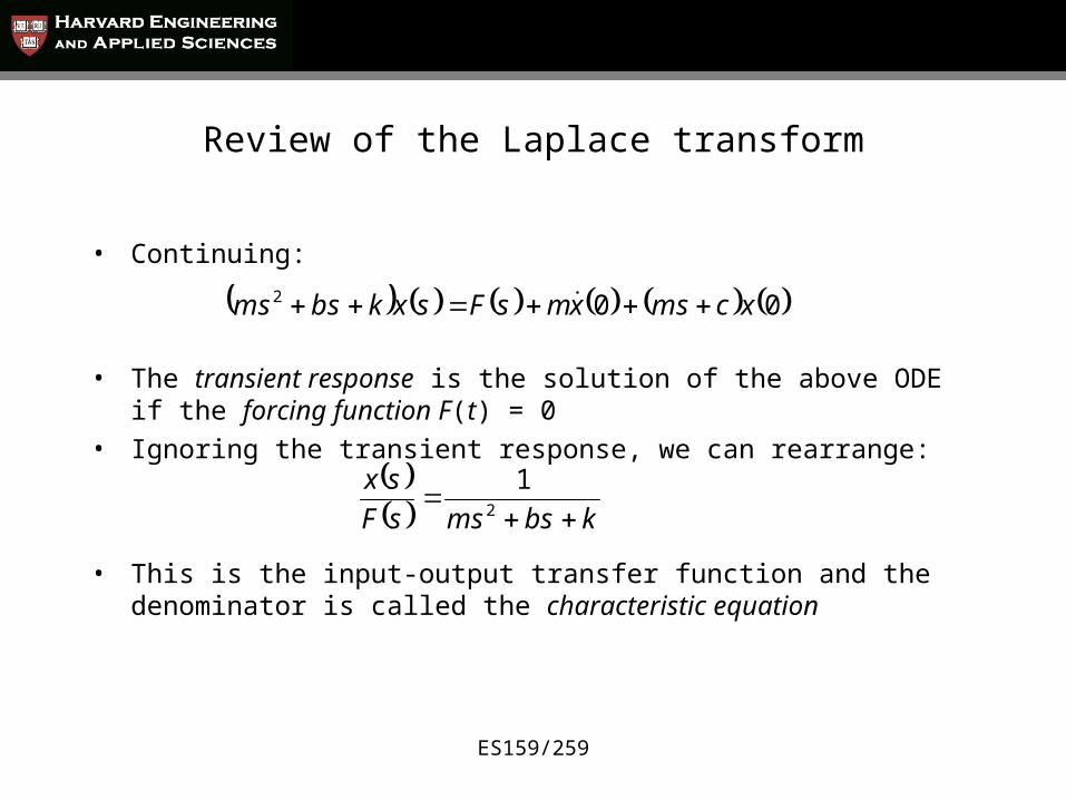
• Continuing:
• The transient response is the solution of the above ODE if the forcing function F(t) = 0
• Ignoring the transient response, we can rearrange:
• This is the input-output transfer function and the denominator is called the characteristic equation
002 xcmsxmsFsxkbsms
kbsmssF
sx
2
1

ES159/259
Review of the Laplace transform
• Properties of the Laplace transform– Takes an ODE to a algebraic equation– Differentiation in the time domain is multiplication by s in the Laplace
domain– Integration in the time domain is multiplication by 1/s in the Laplace domain– Considers initial conditions
• i.e. transient and steady-state response
– The Laplace transform is a linear operator

ES159/259
Review of the Laplace transform
• for this class, we will rely on a table of Laplace transform pairs for convenience
Time domain Laplace domain
step
tx
0
dttxetxsx stL
tx 0xssx
tx 002 xsxsxs
Ct 2s
C
s
1
tcos22 s
s
tsin22
s

ES159/259
Review of the Laplace transform
Time domain Laplace domain
tHtx sxe s
txe at asx
atx
C tC
a
sx
a
1

ES159/259
SISO overview
• Typical single input, single output (SISO) system:
• We want the robot tracks the desired trajectory and rejects external disturbances
• We already have the desired trajectory, and we assume that we can measure the actual trajectories
• Thus the first thing we need is a system description

ES159/259
SISO overview
• Need a convenient input-output description of a SISO system
• Two typical representations for the plant:– Transfer function– State-space
• Transfer functions represent the system dynamics in terms of the Laplace transform of the ODEs that represent the system dynamics
• For example, if we have a 1DOF system described by:
• We want the representation in the Laplace domain:
• Therefore, we give the transfer function as:
tBtJt
sBsJs
ssBsJss
2
JBss
J
BsJss
ssP
/
/11

ES159/259
System descriptions
• A generic 2nd order system can be described by the following ODE:
• And we want to get a transfer function representation of the system, take the Laplace transform of both sides:
• Ignoring the transient response, we can rearrange:
• This is the input-output transfer function and the denominator is called the characteristic equation
tFtkxtxbtxm
sFskxxssxbxsxsxsm
tFtxktxbtxm
0002
LLLL
002 xcmsxmsFsxkbsms
kbsmssF
sx
2
1

ES159/259
Example: motor dynamics
• DC motors are ubiquitous in robotics applications
• Here, we develop a transfer function that describes the relationship between the input voltage and the output angular displacement
• First, a physical description of the most common motor: permanent magnet…
am iK 1torque on the rotor:

ES159/259
Physical instantiationstator
rotor(armature)
commutator

ES159/259
Motor dynamics
• When a conductor moves in a magnetic field, a voltage is generated– Called back EMF:
– Where m is the rotor angular velocitymb KV 2
armature inductancearmature resistance
baa VVRi
dt
diL

ES159/259
Motor dynamics
• Since this is a permanent magnet motor, the magnetic flux is constant, we can write:
• Similarly:
• Km and Kb are numerically equivalent, thus there is one constant needed to characterize a motor
amam iKiK 1
dt
dKKV m
bmb
2
torque constant
back EMF constant

ES159/259
Motor dynamics
• This constant is determined from torque-speed curves– Remember, torque and displacement are work conjugates
– 0 is the blocked torque

ES159/259
Single link/joint dynamics
• Now, lets take our motor and connect it to a link
• Between the motor and link there is a gear such that:
• Lump the actuator and gear inertias:
• Now we can write the dynamics of this mechanical system:
Lm r gam JJJ
riK
rdt
dB
dt
dJ L
amL
mm
mm
m
2
2

ES159/259
Motor dynamics
• Now we have the ODEs describing this system in both the electrical and mechanical domains:
• In the Laplace domain:r
iKdt
dB
dt
dJ L
amm
mm
m
2
2
dt
dKVRi
dt
diL m
baa
r
ssIKssBsJ L
ammmm
2
ssKsVsIRLs mba

ES159/259
Motor dynamics
• These two can be combined to define, for example, the input-output relationship for the input voltage, load torque, and output displacement:

ES159/259
Motor dynamics
• Remember, we want to express the system as a transfer function from the input to the output angular displacement
– But we have two potential inputs: the load torque and the armature voltage
– First, assume L = 0 and solve for m(s):
sIK
ssBsJa
m
mmm 2 ssKsVs
K
sBsJRLsmbm
m
mm 2
mbmm
mm
KKBsJRLss
K
sV
s

ES159/259
Motor dynamics
• Now consider that V(s) = 0 and solve for m(s):
• Note that this is a function of the gear ratio– The larger the gear ratio, the less effect external torques have on the
angular displacement
mbmmL
m
KKBsJRLss
rRLs
s
s
/
RLs
ssKsI mb
a
r
s
RLs
ssKKssBsJ Lmbm
mmm
2

ES159/259
Motor dynamics
• In this system there are two ‘time constants’– Electrical: L/R
– Mechanical: Jm/Bm
• For intuitively obvious reasons, the electrical time constant is assumed to be small compared to the mechanical time constant
– Thus, ignoring electrical time constant will lead to a simpler version of the previous equations:
RKKBsJs
r
s
s
mbmmL
m
/
/1
RKKBsJs
RK
sV
s
mbmm
mm
/
/

ES159/259
Motor dynamics
• Rewriting these in the time domain gives:
• By superposition of the solutions of these two linear 2nd order ODEs:
RKKBsJs
r
s
s
mbmmL
m
/
/1
RKKBsJs
RK
sV
s
mbmm
mm
/
/
tVRKtRKKBtJ mmmbmmm //
tRtRKKBtJ Lmmbmmm /1/
tRtVRKtRKKBtJ Lmmmbmmm /1//
J B tu td

ES159/259
Motor dynamics
• Therefore, we can write the dynamics of a DC motor attached to a load as:
– Note that u(t) is the input and d(t) is the disturbance (e.g. the dynamic coupling from motion of other links)
• To represent this as a transfer function, take the Laplace transform:
tdtutBtJ
sDsUsBsJs 2
ES159/259
Setpoint controllers
• We will first discuss three initial controllers: P, PD and PID– Both attempt to drive the error (between a desired trajectory and the actual
trajectory) to zero
• The system can have any dynamics, but we will concentrate on the previously derived system

Proportional Controller
ES159/259
teKtu p
tEKsU p
• Control law:
– Where e(t) = d(t) - (t)
• in the Laplace domain:
• This gives the following closed-loop system:
pK

ES159/259
PD controller
• Control law:
– Where e(t) = d(t) - (t)
• in the Laplace domain:
• This gives the following closed-loop system:
teKteKtu dp
tEsKKsU dp

ES159/259
PD controller
• This system can be described by:
• Where, again, U(s) is:
• Combining these gives us:
• Solving for gives:
BsJs
sDsUs
2
sssKKsU ddp
BsJs
sDsssKKs
ddp
2
pd
ddp
ddppd
ddpdp
KsKBJs
sDssKKs
sDssKKsKsKBJs
sDssKKssKKsBsJs
2
2
2

ES159/259
PD controller
• The denominator is the characteristic polynomial• The roots of the characteristic polynomial determine the performance of
the system
• If we think of the closed-loop system as a damped second order system, this allows us to choose values of Kp and Kd
• Thus Kp and Kd are:
• A natural choice is = 1 (critically damped)
02
J
Ks
J
KBs pd
02 22 ss
BJK
JK
d
p
2
2

ES159/259
PD controller
• Limitations of the PD controller:– for illustration, let our desired trajectory be a step input and our disturbance
be a constant as well:
– Plugging this into our system description gives:
– For these conditions, what is the steady-state value of the displacement?
– Thus the steady state error is –D/Kp
– Therefore to drive the error to zero in the presence of large disturbances, we need large gains… so we turn to another controller
s
DsD
s
Csd ,
pd
dp
KsKBJss
DCsKKs
2
pp
p
pd
dp
spd
dp
sss K
DC
K
DCK
KsKBJs
DCsKK
KsKBJss
sDCsKKs
2020limlim
ES159/259
PID controller
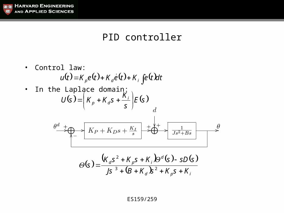
• Control law:
• In the Laplace domain:
dtteKteKteKtu idp
sEs
KsKKsU i
dp
ipd
dipd
KsKsKBJs
ssDsKsKsKs
23
2

ES159/259
PID controller
• The integral term eliminates the steady state error that can arise from a large disturbance
• How to determine PID gains1. Set Ki = 0 and solve for Kp and Kd
2. Determine Ki to eliminate steady state error
• However, we need to be careful of the stability conditions
J
KKBK pd
i
ES159/259
PID controller
• Stability– The closed-loop stability of these systems is determined by the roots of the
characteristic polynomial– If all roots (potentially complex) are in the ‘left-half’ plane, our system is
stable• for any bounded input and disturbance
– A description of how the roots of the characteristic equation change (as a function of controller gains) is very valuable
• Called the root locus

Summary• Proportional
– A pure proportional controller will have a steady-state error– Adding a integration term will remove the bias– High gain (Kp) will produce a fast system– High gain may cause oscillations and may make the system unstable– High gain reduces the steady-state error
• Integral– Removes steady-state error– Increasing Ki accelerates the controller– High Ki may give oscillations– Increasing Ki will increase the settling time
• Derivative– Larger Kd decreases oscillations– Improves stability for low values of Kd
– May be highly sensitive to noise if one takes the derivative of a noisy error– High noise leads to instability
ES159/259


