

Udo Ebert*
Ethical inequality measures and the redistribution of income when needs differ
January 2005
* Address: Department of Economics, University of Oldenburg, D-26111 Oldenburg, Germany
Tel.: (+49)441-798-4113
Fax: (+49)441-798-4116
e-mail: [email protected]

Abstract
The paper considers social welfare functions and ethical inequality measures for linear
inequality concepts when households may differ in needs. The welfare functions are nested,
i.e. separable in the level of welfare attained by the homogeneous subpopulations, and possess
a homogeneity property depending on the inequality concept imposed. Several principles of
transfers between different household types are introduced and systematically examined.
Their implications for the form of welfare functions and inequality measures are derived. The
corresponding classes are completely described.
Keywords: Welfare functions, inequality measures, inequality concepts, differences in needs,
transfer principles, axiomatization.
JEL codes: D63, I31

- 1 -
1. Introduction1
The principle of progressive transfers postulates that the redistribution of (a small amount of)
income from a richer individual to a poorer one increases the level of social welfare and
decreases the degree of inequality. The idea goes back to Pigou and was generalized by
Dalton (1920). The principle is without doubt the foundation stone of a normative theory of
redistribution: Whenever one income distribution is more equal than another one (with the
same average income) – measured by Lorenz dominance, it can be generated by a finite series
of progressive transfers from the original income distribution. In this case, however, the indi-
viduals considered have to be identical in every respect but possibly income. Things become
much more complicated if we assume that the economic units under consideration may also
differ with respect to further attributes: For instance households can have different size or
needs. Then it is not at all clear what kind of income transfer may improve welfare and
equality since two variables – income and needs – have to be taken into account. Furthermore,
the concept of inequality used has to be taken into consideration, as well.
The objective of this paper is to investigate some principles of redistribution in a hetero-
geneous framework systematically and to discuss their implications for the measurement of
welfare. Moreover we translate these results to the measurement of inequality and derive the
corresponding ethical inequality measures. We also examine various inequality concepts. The
underlying framework can be described simply: a typical household can be characterized by
its income and its type. (Both variables can in principle be observed!) We assume throughout
the paper that household types can be ranked by needs.
Then a transfer principle has at first to compare the situation of the households involved:
which one is ‘richer’, and which one ‘poorer’? Here the notions of ‘rich’ and ‘poor’ have to
take into consideration the living standards, i.e. the level of income and the household’s
needs. Thus the principles crucially depend on the comparability of these information. The
weakest principle is only able to compare the level of income and needs separately, i.e. a
household can be identified as the ‘richer’ one if its income is higher and if it is less needy.
Thus the ranking of living standards is a dominance criterion and is incomplete. The strongest
one is able to compare the situation of households with arbitrary incomes and needs. Here a
complete ordering of the living standard of households is given. Between these extremes two
further possibilities are discussed. Then in a second step, when the measuring of ‘richer’ and
‘poorer’ has been clarified, the transfer itself has to be defined. 1 I would like to thank Patrick Moyes for helpful comments.

- 2 -
We examine a general class of social welfare orderings. The corresponding welfare functions
are nested: at first the level of welfare of all households having the same type is determined.
Then these welfare levels are aggregated to an overall welfare ordering in the second step.
This class contains the set of separable welfare functions as proper subclass. Since ethical
inequality measures are to be derived, the welfare orderings have to possess an appropriate
homogeneity property depending on the inequality concept chosen. In the paper we consider
linear inequality concepts (which are the only coherent inequality views, cf. Ebert (2004)), i.e.
we derive measures according to the relative, absolute, intermediate, and reference-point
inequality view.
The transfer principles introduced have different power. The weakest one only assumes that
income and needs can be ranked. Another one allows to compare the income of different
household types by using one-sided bounds. A third one is based on two-sided bounds.
Finally, the strongest principle is formulated on the basis of an equivalent income function. It
corresponds to the between-type transfer principle used in the literature. The transfer prin-
ciples are imposed in two different ways: at first only transfers between two particular house-
hold types are considered. In a second step transfers between arbitrary subpopulations are
admitted. The implications of these principles for the form of welfare orderings and inequality
measures are derived for a fixed population. Furthermore, depending on the transfer principle
imposed the corresponding classes are described completely. As expected, the weaker the
transfer axiom the greater is the corresponding class of measures. We obtain some classes
which have not yet been presented in the literature.
There are few papers dealing with this topic: Ebert (1995) introduces one generalized Pigou-
Dalton principle for the measurement of relative inequality. Ebert (1997) is concerned with an
analogous principle for absolute inequality. Shorrocks (1995) is primarily interested in some
(incomplete) welfare and inequality orderings. In Ebert (2004) a different approach is used:
here equivalent income functions and weights reflecting the type of household are given a
priori and then a between-type transfer principle is imposed on a class of welfare and
inequality orderings. To sum up, a systematic and general analysis of transfer principles for
linear inequality concepts is still missing.
The paper is organized as follows: Section 2 introduces the notation. Section 3 presents the
framework. In section 4 the transfer principles are defined and discussed. Their implications
are investigated. Section 5 concludes.

- 3 -
2. Notation
We investigate a heterogeneous population. There are 2n ≥ types of household having
different composition and/or needs. So we face n homogeneous subpopulations. We will
assume that a household of type i comprises i adults, but this assumption is not necessary.
Each subpopulation , 1,...,i i n= , consists of in households of type i. The total number of
households is denoted by 1
:n
ii
N n=
= ∑ . It is important that the household types can be ranked
by needs. They are numbered by increasing needs. We assume that the income ijX and the
type i of a household j can be observed. Of course, households can vary in income. Each
income has to be feasible, i.e. ij dX ∈Ω , where ( ),d dΩ = ∞ denotes the set of feasible
incomes. For 0d = we obtain 0 ++Ω = and for d = −∞ the set −∞Ω = . Incomes are either
bounded from below or may be arbitrary. We can interpret d as minimum or reference
income. If income is negative it is assumed that a household is able to survive by getting
credit or by using savings. If ij dX ∈Ω the income i
jX d− is called normalized income for
d ∈ . It is the amount of income of household j measured with respect to the minimum
(reference) income.
Let ( )1 ,..., i
i
ni i in dX X X= ∈Ω denote an income vector of subpopulation i. A vector of incomes
for the overall population is given by ( )1,..., n NX X X= ∈Ω . The average income of X is
denoted by ( ) ijX X Nµ = ΣΣ . Furthermore, let k1 denote a vector of k ones. An ordering
defined on NdΩ is represented by d , where ~d and d denote its symmetric and, respec-
tively, asymmetric part.
3. Welfare and inequality
In the following we describe the framework we are interested in and prove a number of
general results. They will provide the background for the analysis performed in the next
section. At first we will introduce social welfare orderings. Then the class of coherent
inequality concepts is presented and the derivation of ethical inequality measures is discussed.
If an inequality measure has to be consistent with one of the inequality concepts examined,
the underlying welfare ordering has to satisfy a homogeneity property. Therefore the class of
feasible welfare orderings is determined. It turns out that the corresponding welfare functions

- 4 -
are well-structured. They allow us to describe the corresponding class of ethical inequality
orderings/measures precisely.
3.1 Welfare orderings
We will confine ourselves to a particular class of social welfare orderings Wd defined on N
dΩ
which can be represented by nested social welfare functions. Therefore in a first step we
define a social welfare ordering iWd for each subpopulation , 1,...,i i n= . We assume that it
can be represented by
( ) ( )1
1
1 ini i
i i i jji
X V V Xn
ξ −
=
=
∑ (1)
where :i dV Ω → is an increasing, strictly concave household utility function and where
( )1iV t− denotes its inverse function. It turns out that ( )i
i Xξ is the equally distributed equiva-
lent income (EDEI) of iX : if given to each household in subpopulation i this income yields
the same level of welfare as iX . Because of the concavity of iV the ordering iWd satisfies the
(usual) principle of progressive transfers (the subpopulation is homogeneous!). In the second
step we assume that the social welfare ordering Wd is defined on the vector
( ) ( )( )11 ,..., n
nX Xξ ξ and that it can be represented by a welfare function
( ) ( )( )1
1
ni
i i ii
W X V n V Xβ ξ−
=
= ∑ (2)
where V is again strictly increasing and concave, and where 1,..., nβ β are strictly positive
welfare weights. The basic idea underlying this construction can be described as follows: sub-
population i’s EDEI ( )ii Xξ is the representative income of a household of this type. Since
there are in households in this subpopulation (we have to take into account the size of the
subpopulation!) its total contribution to social welfare is ( )( )ii inV Xξ . It is weighted by iβ
which is to reflect the needs of household type i. Furthermore, the welfare function at this
level is also separable. If we replace ( )ii Xξ by its proper definition we see that the welfare

- 5 -
function ( )W X is a nested function having two levels. Since all functions involved are linear
or concave ( )W X is strictly increasing and concave.2
Below, we require a social income function for the definition of ethical inequality orderings.
The function represents the minimal amount of (aggregate) income that is just sufficient to
yield the level of social welfare implied by a given income distribution (if total income is
distributed optimally among households). We define it in analogy to an individual expenditure
function in consumer theory by:
( )11 ,..., 1 1
: mini
nnn
nnij
i j
C Xλ λ
λ= =
= ∑ ∑ (3a)
s.t. ( ) ( )11 ,...,
n
nnW W Xλ λ = . (3b)
Obviously there is a relationship to the concept of EDEI for homogeneous subpopulation. If
there is only one subpopulation the value of the social income function is equal to the EDEI
multiplied by the number of households. It is easy to see that the optimal incomes ijλ , for
1,..., ij n= , have to be identical (since iV is concave). Therefore ( )C X can also be repre-
sented by
( )1,...,
1
minn
n
i ii
C X nλ λ
λ=
= ∑ (4a)
s.t. ( ) ( )11 ,...,
nn n nW W Xλ λ =1 1 . (4b)
3.2 Inequality concepts
Inequality measures (representing inequality orderings) are usually invariant with respect to a
certain type of admissible transformation of incomes. Relative inequality measures do not
change if all incomes are altered proportionally and absolute measures are invariant w.r.t. to
adding the same amount to all incomes. In other words they are consistent with an inequality
concept. We will examine the class of coherent inequality concepts (Ebert (2004a)). They
have to satisfy two properties: path-independence and transfer-consistency. The first one
requires that the composition of two admissible transformations is also admissible. Then 2 Another possibility of defining an ordering W
d is to use a separable welfare function from the beginning and
to consider ( ) ( )( )1 ii jW X V V X−= ΣΣ . Then there is only one level. It turns out that both forms coincide if
and only if we define ( ) ( )i iV t V tβ= for 1, ...,i n= .

- 6 -
‘having the same degree of inequality’ is a transitive relation. The second one postulates that
if a (sequence of) progressive transfers is needed in order to obtain one distribution from
another one, then so it is the case after applying the same admissible transformation to both
distributions. It requires that a change in the size of incomes (admissible transformation) and a
redistribution of income are compatible with one another. This criterion implies in particular
that Lorenz dominance (appropriately defined) is preserved if the distributions involved are
transformed by admissible transformations.
It turns out that there is exactly one coherent inequality concept dJ for every NdΩ . The
admissible transformations have to be linear. We obtain the functions
( ) ( )dT t t d dλ λ= − + for dt∈Ω and λ ++∈ if d ∈ and (5a)
( )T t tα α−∞ = + for t −∞∈Ω and α ∈ if d = −∞ (5b)
which define the transformations
( ) ( ) ( )( )11: ,...,
n
d d d nnT X T X T Xλ λ λ= and ( ) ( ) ( )( )1
1: ,...,n
nnT X T X T Xα α α
−∞ −∞ −∞= .
For 0d = and d = −∞ we get the relative and, respectively, absolute inequality concept, for
0d < the intermediate one and for 0d > reference-point inequality. They are discussed in
more detail in Ebert (2004a).
3.3 Ethical inequality orderings
Ethical inequality orderings are derived from social welfare orderings. Suppose that Wd is a
social welfare ordering for d ∈ . Then a corresponding inequality ordering Id can be
defined by means of the relative welfare loss due to inequality. It is calculated on the basis of
the normalized income per household:
( ) ( )( ) ( )( )( )
:d
X d C X N dI X
X dµ
µ− − −
=−
for d ∈ . (6a)
Similarly, we consider the absolute welfare loss per household for d = −∞
( ) ( ) ( )I X X C X Nµ−∞ = − . (6b)
These indicators determine the corresponding inequality orderings uniquely.
But the orderings have to be consistent ( dJ -invariant) with the inequality concept dJ , i.e.

- 7 -
( )~ I ddX T Xλ for all N
dX ∈Ω and if dλ ++∈ ∈ (7a)
and
( )~ I dX T Xα−∞ for NdX ∈Ω and α ∈ . (7b)
We call a social welfare ordering dJ -homogeneous with respect to the admissible trans-
formations if for all , NdX Y ∈Ω :
( ) ( )~ ~W d W dd dX Y T X T Yλ λ⇔ for all λ ++∈ if d ∈ (8a)
and, respectively,
( ) ( )~ ~W WX Y T X T Yα α−∞ −∞
−∞ −∞⇔ for all α ∈ if d = −∞ (8b)
and get3
Proposition 1
Id is dJ -invariant if and only if the corresponding ordering W
d is dJ -homogeneous.
Therefore dJ -homogeneity is a crucial property of the welfare orderings we want to consider.
3.4 Homogeneous welfare orderings
We restrict ourselves to the class of dJ -homogeneous welfare orderings which can be
described precisely:
Proposition 2
a) Wd is dJ -homogeneous if and only if iW
d and the overall ordering defined on
( ) ( )( )11 ,..., n
nX Xξ ξ are dJ -homogeneous.
b) For d ∈ : Wd is dJ -homogeneous if and only if there are ( )1, ,..., ,1nε ε ε ∈ ∞ and
1 21, ,..., nβ β β ++= ∈ such that Wd is represented by4
( ) ( )1
1 1
1 ii
inn
ii id j
i jh h i
nW X X d dn n
εε εεβ
β= =
= − + Σ ∑ ∑ for N
dX ∈Ω . (9a)
3 All proofs have been relegated to the Appendix. 4 If an exponent is equal to zero we have to use the corresponding geometric mean.
- 8 -
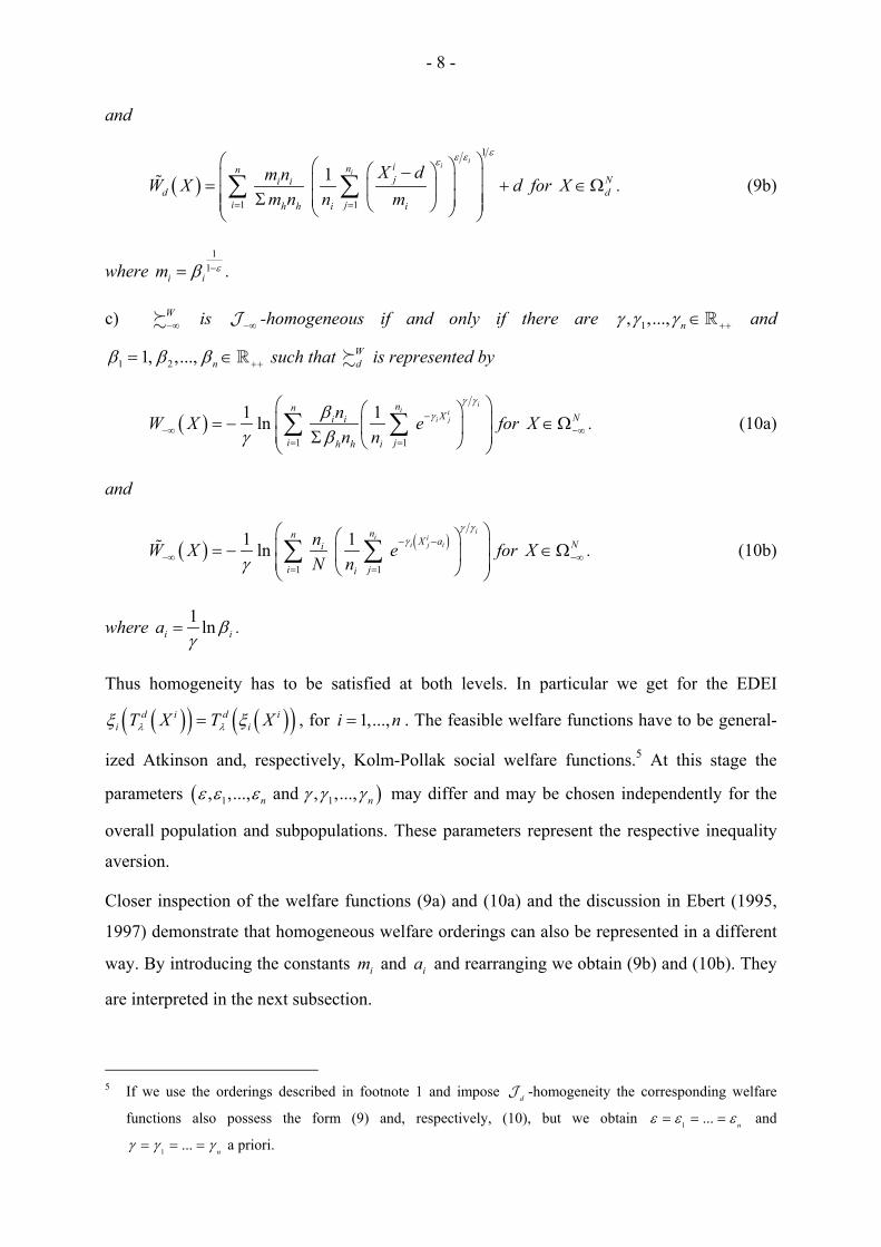
and
( )
1
1 1
1i
ii inn
ji id
i jh h i i
X dm nW X dm n n m
εε εε
= =
− = + Σ ∑ ∑ for N
dX ∈Ω . (9b)
where 1
1i im εβ −= .
c) W−∞ is −∞J -homogeneous if and only if there are 1, ,..., nγ γ γ ++∈ and
1 21, ,..., nβ β β ++= ∈ such that Wd is represented by
( )1 1
1 1lni
i ii j
nnXi i
i jh h i
nW X en n
γ γγβ
γ β−
−∞= =
= − Σ ∑ ∑ for NX −∞∈Ω . (10a)
and
( ) ( )1 1
1 1lni
i ii j i
nnX ai
i ji
nW X eN n
γ γγ
γ− −
−∞= =
= − ∑ ∑ for NX −∞∈Ω . (10b)
where 1 lni ia βγ
= .
Thus homogeneity has to be satisfied at both levels. In particular we get for the EDEI
( )( ) ( )( )d i d ii iT X T Xλ λξ ξ= , for 1,...,i n= . The feasible welfare functions have to be general-
ized Atkinson and, respectively, Kolm-Pollak social welfare functions.5 At this stage the
parameters ( )1 1, ,..., and , ,...,n nε ε ε γ γ γ may differ and may be chosen independently for the
overall population and subpopulations. These parameters represent the respective inequality
aversion.
Closer inspection of the welfare functions (9a) and (10a) and the discussion in Ebert (1995,
1997) demonstrate that homogeneous welfare orderings can also be represented in a different
way. By introducing the constants im and ia and rearranging we obtain (9b) and (10b). They
are interpreted in the next subsection.
5 If we use the orderings described in footnote 1 and impose dJ -homogeneity the corresponding welfare
functions also possess the form (9) and, respectively, (10), but we obtain 1 ... nε ε ε= = = and
1 ... nγ γ γ= = = a priori.
- 9 -
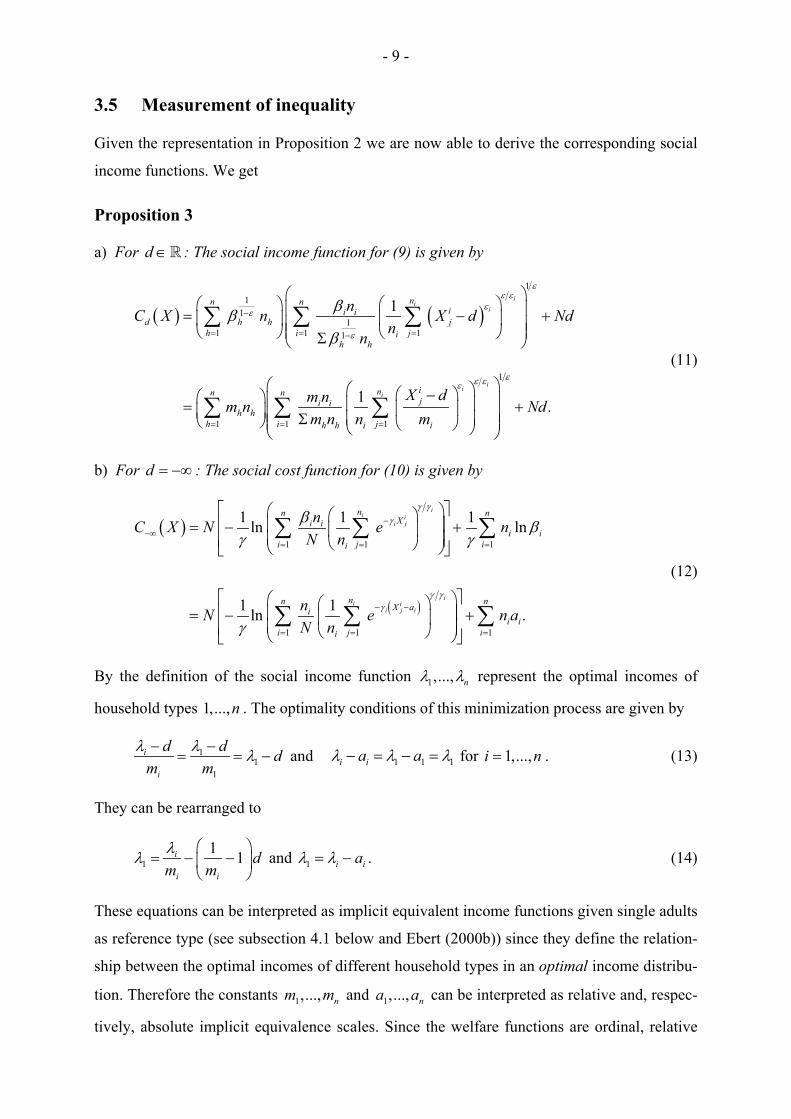
3.5 Measurement of inequality
Given the representation in Proposition 2 we are now able to derive the corresponding social
income functions. We get
Proposition 3
a) For d ∈ : The social income function for (9) is given by
( ) ( )1
11
11 1 11
1
1 1 1
1
1 .
ii
i
iii
nn nii i
d h h jh i ji
h h
inn nji i
h hh i jh h i i
nC X n X d Ndnn
X dm nm n Ndm n n m
εε ε
εε
ε
εε εε
βββ
−
= = =−
= = =
= − + Σ
− = + Σ
∑ ∑ ∑
∑ ∑ ∑
(11)
b) For d = −∞ : The social cost function for (10) is given by
( )
( )
1 1 1
1 1 1
1 1 1ln ln
1 1ln .
ii i
i j
ii i
i j i
nn nXi i
i ii j ii
nn nX ai
i ii j ii
nC X N e nN n
nN e n aN n
γ γγ
γ γγ
β βγ γ
γ
−−∞
= = =
− −
= = =
= − +
= − +
∑ ∑ ∑
∑ ∑ ∑
(12)
By the definition of the social income function 1,..., nλ λ represent the optimal incomes of
household types 1,...,n . The optimality conditions of this minimization process are given by
11
1
i
i
d d dm m
λ λ λ− −= = − and 1 1 1i ia aλ λ λ− = − = for 1,...,i n= . (13)
They can be rearranged to
11 1i
i i
dm mλλ
= − −
and 1 i iaλ λ= − . (14)
These equations can be interpreted as implicit equivalent income functions given single adults
as reference type (see subsection 4.1 below and Ebert (2000b)) since they define the relation-
ship between the optimal incomes of different household types in an optimal income distribu-
tion. Therefore the constants 1,..., nm m and 1,..., na a can be interpreted as relative and, respec-
tively, absolute implicit equivalence scales. Since the welfare functions are ordinal, relative

- 10 -
scales are unique up to a scale factor; absolute scales can be changed by adding a constant.
Therefore, without loss of generality we can choose household type 1 (single adults) as
reference type by setting 1 1m = and 1 0a = . ( )ij iX d m− and, respectively, i
j iX a− then
represents the implicit equivalent income of a representative equivalent adult in household j of
type i. For , 0d d∈ ≠ we get a combination of relative and absolute scales.
Using the definition of inequality measures presented in subsection 3.3 and the result of
Proposition 3 we are now able to describe the inequality orderings more precisely.
Proposition 4
The social welfare functions (9) and (10) imply
( ) ( )
1
1 1
11ii
i innji i
d di jh h i i
X dm nI X Xm n n m
εε εε
µ= =
− = − Σ ∑ ∑ (15)
and
( ) ( ) ( )1 1
1 1lni
i ii j i
nnX ai
i ji
nI X X eN n
γ γγµ
γ− −
−∞ −∞= =
= + ∑ ∑ (16)
where
( )1 1
i innji
di j h h i
X dmXm n m
µ= =
−= Σ ∑ ∑ and ( ) ( )
1 1
1 innij i
i j
X X aN
µ−∞= =
= −∑ ∑ , (17) + (18)
respectively.
We will come back to these representations of the inequality measures in section 5. Now we
turn to a systematic discussion of transfer principles and of their implications.
4. Redistribution
The starting point of the following analysis is the Pigou-Dalton principle for homogeneous
populations. It requires that a progressive transfer (i.e. a transfer from a richer to a poorer
individual which does not reverse the ranking of incomes) improves social welfare (and
decreases inequality). In our framework things are more complicated since the households
belonging to different subpopulations have different needs. These differences in needs have to
be taken into account, as well, when income is redistributed.

- 11 -
In this section we will introduce four different types of progressive transfers between different
subpopulations. They will differ with respect to the assumption made on the comparability of
living standards which depend on income and needs.
4.1 Transfer principles
The first kind of transfer takes into account only the ranking of income and needs. We intro-
duce
WBT(d) A transfer of income 0δ > changing ikX to i
kX δ− and 1ilX + to 1i
lX δ+ + is a
Weak Between-Type Progressive Transfer if 1i ik lX Xδ δ+− > + .
The transfer redistributes income from a less needy and richer household to a needier and
poorer household such that after redistributing income the first one is still richer than the
second one. Here only information about the ranking of income and needs is required. Needs
are not compared in a cardinal manner and it is clear that after the redistribution of income the
household receiving the transfer is still worse off than the other one. The richer household is
definitely better off than the poorer one, i.e. its income is higher and it is less needy. The
definition can be employed for any d ∈ and d = −∞ . Furthermore, the condition compar-
ing incomes is equivalent to a formulation based on normalized incomes:
( ) ( )1i ik lX d X dδ δ+− − > + − for d ∈ . (19)
This kind of transfer is similar to Hammond’s equity principle (which is applied to utility
levels; cf. Hammond (1976)). It is identical with the transfer P3 used in Ebert (2000a) and
also plays a role in Bourguignon (1989).
Sometimes one is willing to compare the living standards of households belonging to different
subpopulations ‘a little bit’; a(n upward) transfer from a household of type i to a household of
type 1i + may even be desirable if the income of the recipient is a bit higher in the end than
the income of the donor. The problem is to define the term ‘a bit higher’. Formally we intro-
duce
UBT(d) Assume that 1ir < . A transfer of income 0δ > changing ikX to i
kX δ− and 1ilX + to
1ilX δ+ + is an Upward Between-Type Progressive Transfer if
( ) ( )1i ik i lX d r X dδ δ+ − − > + − .

- 12 -
In this case the constant ir determines the term ‘a bit’ precisely (in a relative way, i.e. by a
ratio of incomes). The definition of this transfer is based on normalized income and is valid
for d ∈ . For d = −∞ we define
UBT(−∞ ) Assume that 0ib < . A transfer of income 0δ > changing ikX to i
kX δ− and 1ilX +
to 1ilX δ+ + is an Upward Between-Type Progressive Transfer if
( ) ( )1i ik l iX X bδ δ+− > + + .
Here the constant ib determines the bound.
If 1ir = or 0ib = the transfer UBT(d) coincides with WBT(d). Thus an upward between-type
progressive transfer is an extension of the latter type of transfer. It is easy to see that constants
ir or ib can really be chosen in practice. For instance two adults need a higher level of income
than a single adult in order to be as well off. A constant 10 11ir = means that a transfer from
the single to the couple is admissible as long as the couple’s (resulting) income is less than
110 % of the single person’s income.
If a needier household’s income is high enough we can also redistribute income to a less
needy one. E.g. if a couple’s income is (more than) twice as high as a single adult’s income it
seems to be better off. Therefore we introduce
DBT(d) Assume that 1is > . A transfer of income 0δ > changing 1ilX + to 1i
lX δ+ − and ikX
to ikX δ+ is a Downward Between-Type Progressive Transfer if
( ) ( )1i il i kX d s X dδ δ+ − − > + −
for d ∈ and
DBT(−∞ ) Assume that 0ic > . A transfer of income 0δ > changing 1ilX + to 1i
lX δ+ − and
ikX to i
kX δ+ is a Downward Between-Type Progressive Transfer if
( ) ( )1i il k iX X cδ δ+ − > + + .
The interpretation of this kind of transfer is analogous.

- 13 -
Finally we assume that we are able to compare living standards completely. Suppose that an
equivalent income function6 E is explicitly defined in the following way: Choosing household
type 1 (single adults) as reference type we introduce an equivalent income function E as a
vector of n functions :i d dE Ω →Ω , where ( )iE t denotes the income a single adult requires
in order to be as well off as a household with i adults and household income t. (Here it is
assumed implicitly that all members belonging to a household attain the same living
standard.) The functions iE have to satisfy some properties which allow us to make meaning-
ful comparisons.
(i) ( )1E t t=
(ii) ( )iE t is continuous and strictly increasing in t
(iii) ( )iE t is strictly decreasing in i
(iv) ( )iE t is an invertible function.
For an interpretation of these properties see e.g. Ebert (2000b).
( )iE t is called equivalent income. Then a household of type i is better off than a household of
type h if and only if ( ) ( )i hi j h kE X E X> for any , 1,...,h i n∈ . If ( ) ( )i h
i j h kE X E X= the living
standards are the same. When an equivalent income function is given the living standards
(equivalent incomes) of arbitrary households and household types can be compared. Then we
define an appropriate transfer for d ∈ or d = −∞ by
SBT(d) A transfer of income 0δ > changing ikX to i
kX δ− 1 1 to i il lX X δ+ + − and 1i
lX + to
1ilX δ+ + to i i
k kX X δ + is a Strong Between-Type Progressive Transfer if
( ) ( )11
i ii k i lE X E Xδ δ+
+− > + ( ) ( )11
i ii l i kE X E Xδ δ++
− > + .
It is the ‘usual’ Between-Type Progressive Transfer used in the literature (see e.g. Ebert
(2004b)).
After having introduced four different kinds of transfers we define the corresponding
Principles of Transfers which will be denoted by the same acronyms. They require that the
respective transfer improves social welfare (and decreases inequality).
6 See Donaldson and Pendakur (2004)

- 14 -
In the following we will always assume that the social welfare ordering Wd can be repre-
sented by a welfare function satisfying (9a) and, respectively, (10a). The implications for the
representation (9b) and (10b) are discussed in section 5.
4.2 Two subpopulations
Since we want to analyze the implications of the transfer principles in detail we at first
consider two subpopulations i and 1i + . It is clear that the results depend on the principle
chosen and the inequality concept considered. The latter determines a class of feasible social
welfare orderings (see Proposition 2). Given this class of welfare orderings and the social
welfare functions which represent them we can describe the implications of a transfer
principle by two conditions: The parameters ( 1, ,i iε ε ε + and, respectively, 1, ,i iγ γ γ + ) have to be
related and we obtain a condition on the weights 1,i iβ β + .
(a) Principle WBT
Starting with d ∈ we obtain
Proposition 5a
Wd satisfies WBT(d) for d ∈ if and only if
[ 1i iε ε ε+ ≤ ≤ for 1 0iε + > , (20a)
1 0i iε ε ε+ = ≤ < for 1 0iε + ≤ and 0iε > (20b)
1i iε ε ε+ = = for 1 0iε + ≤ and 0iε ≤ , (20c)
and
1
1
11
1 1i i
i i
i ii in n
ε ε ε εε ε
β β+
+
− −
++
≤
].
In this case we have to distinguish several cases as far as the parameters are concerned: It
turns out that the parameter (inequality aversion) of the receiver 1iε + must not exceed (be
higher than) the parameter (inequality aversion) of the total population ε which in turn must
be less (higher) than or equal to the donor’s parameter (inequality aversion) iε . In other words
the inequality aversion of the needier subpopulation has to be weakly higher than the aversion
of the less needy one. This is true as long as the parameters are strictly positive. If at least one

- 15 -
is nonpositive, two or all three parameters have to be identical. Otherwise it is impossible to
satisfy WBT(d). Furthermore we get a condition on the weights iβ and 1iβ + . It may also
depend on the size of the subpopulations involved. The condition requires that the weight of
the needier subpopulation is greater than the other one.
For d = −∞ we obtain a clearer result:
Proposition 5b
Wd satisfies WBT ( )−∞ if and only if 1i iγ γ γ += = and 1i iβ β +≤ .
In this case all parameters have to be identical and the coefficients have to be nondecreasing
in needs.
(b) Principle UBT
We know that UBT is a more general transfer principle than WBT since here an additional
bound is given. In this case the conditions on the weights iβ and 1iβ + are stricter:
Proposition 6
a) Wd satisfies UBT(d) for d ∈ if and only if (20) and
1
1 11
1
1 1i i
i i
i i ii i
rn n
ε ε ε εε ε
εβ β+
+
− −
−+
+
≤
.
b) Wd satisfies UBT(−∞ ) if and only if 1i iγ γ γ += = and 1
i ibi ieγβ β +≤ .
Since 1ir < and 0ib < the increase of 1iβ + measured with respect to iβ has to be even larger
than above.
(c) Principle DBT
As one would expect the results for downward transfers are essentially analogous. We have to
replace (20) by
1i iε ε ε +≤ ≤ for 0iε > (21a)
10i iε ε ε += ≤ < for 0iε ≤ and 1 0iε + > (21b)
1i iε ε ε += = for 0iε ≤ and 1 0iε + ≤ . (21c)
Then we obtain
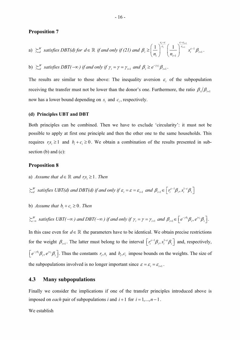
- 16 -
Proposition 7
a) Wd satisfies DBT(d) for d ∈ if and only if (21) and
1
1 11
1
1 1i i
i i
i i ii i
sn n
ε ε ε εε ε
εβ β+
+
− −
−+
+
≥
.
b) Wd satisfies DBT(−∞ ) if and only if 1i iγ γ γ += = and 1
i ici ie γβ β−
+≥ .
The results are similar to those above: The inequality aversion iε of the subpopulation
receiving the transfer must not be lower than the donor’s one. Furthermore, the ratio 1i iβ β +
now has a lower bound depending on is and ic , respectively.
(d) Principles UBT and DBT
Both principles can be combined. Then we have to exclude ‘circularity’: it must not be
possible to apply at first one principle and then the other one to the same households. This
requires 1i ir s ≥ and 0i ib c+ ≥ . We obtain a combination of the results presented in sub-
section (b) and (c):
Proposition 8
a) Assume that d ∈ and 1i ir s ≥ . Then
Wd satisfies UBT(d) and DBT(d) if and only if 1i iε ε ε += = and 1 1
1 ,i i i i ir sε εβ β β− −+ ∈
b) Assume that 0i ib c+ ≥ . Then
W−∞ satisfies UBT(−∞ ) and DBT(−∞ ) if and only if 1i iγ γ γ += = and 1 ,i ib c
i i ie eγ γβ β β−+ ∈ .
In this case even for d ∈ the parameters have to be identical. We obtain precise restrictions
for the weight 1iβ + . The latter must belong to the interval 1 1,i i i ir sε εβ β− − and, respectively,
,i ib ci ie eγ γβ β− . Thus the constants ,i ir s and ,i ib c impose bounds on the weights. The size of
the subpopulations involved is no longer important since 1i iε ε ε += = .
4.3 Many subpopulations
Finally we consider the implications if one of the transfer principles introduced above is
imposed on each pair of subpopulations i and 1i + for 1,..., 1i n= − .
We establish

- 17 -
Proposition 6* [7*]
a) Wd satisfies UBT(d) [DBT(d)] for 1,..., 1i n= − and d ∈ if and only if
( 1 2 1...n nε ε ε ε ε−≤ = = = ≤ for 0nε >
or 1 2 1...n nε ε ε ε ε−= = = = ≤ for 0nε ≤ and 1 0ε >
or 1 ... nε ε ε= = = otherwise)
[ 1 2 1... n nε ε ε ε ε−≤ = = = ≤ for 1 0ε >
or 1 2 2... nε ε ε ε ε= = = = ≤ for 1 0ε ≤ and 0nε >
or 1 ... nε ε ε= = = otherwise]
and
1
1 1 11 1 2 1
1
1( , i i ir rn
ε εε
ε εβ β β β
−
− −+
≤ ≤
for 2,..., 2,i n= − and 11 1
1n
n
n n nn
rn
ε εε
εβ β
−
−− −
≤
)
1
1 1 11 1 2 1
1
1[ , i i is sn
ε εε
ε εβ β β β
−
− −+
≥ ≥
for 2,..., 2,i n= − and 11 1
1n
n
n n nn
sn
ε εε
εβ β
−
−− −
≥
].
b) W−∞ satisfies UBT(−∞ ) [DBT(−∞ )] for 1,..., 1i n= − if and only if
1 ... nγ γ γ= = = and
1i ib
i ieγβ β +≤ for 1,..., 1i n= −
[ 1i ic
i ie γβ β−+≥ for 1,..., 1i n= − ].
This proposition is easily proved by repeated application of the respective results derived in
subsection 4.2. It is important to note that Proposition 6* also presents the outcome for an
application of WBT(d) and WBT(−∞ ) (set 1ir ≡ and 0ib ≡ ). It turns out that the parameters
iε have to be identical to ε for 2,..., 1i n= − (since these subpopulations may be the receiver
and the donor of a transfer). The inequality aversion for the neediest and least needy sub-
population may differ from ε . If UBT(d) and DBT(d) are applied simultaneously (for d ∈ )
this property vanishes. We obtain
Proposition 8*
a) Assume that d ∈ and 1, 1, 1i i i ir s rs< > ≥ for 1,...,i n= .

- 18 -
Wd satisfies UBT(d) and DBT(d) for 1,..., 1i n= − if and only if 1 ... nε ε ε= = = and
1 11 ,i i i i ir sε εβ β β− −+ ∈ for 1,..., 1i n= − .
b) Assume that 0, 0, 0i i i ib c b c< > + ≥ .
W−∞ satisfies UBT(−∞ ) and DBT(−∞ ) for 1,..., 1i n= − if and only if 1 ... nγ γ γ= = = and
1 ,i ib ci i ie eγ γβ β β−+ ∈ for 1,..., 1i n= − .
Proposition 8* extends the results derived in Ebert (1995, 1997) to inequality concepts 0d ≠
and d ≠ −∞ .
Finally we examine the Strong Between-Type Transfer Principle. In this case the living
standard of arbitrary subpopulations can be compared. We get
Proposition 9
a) Wd satisfies SBT(d) for 1,..., 1i n= − and d ∈ if and only if 1 ... nε ε ε= = = ,
1 21 ... nβ β β= ≤ ≤ ≤ , and ( ) ( )1i iE t t d dεβ −= − + for 1,...,i n= .
b) W−∞ satisfies SBT(−∞ ) for 1,..., 1i n= − if and only if 1 ... nγ γ γ= = = , 1 21 ... nβ β β≤ ≤ ≤ ,
and ( ) 1 lni iE t t βγ
= − for 1,...,i n= .
In this case the welfare ordering and the equivalent income function used in the transfer
principle SBT are closely related. One has to employ relative and, respectively, absolute
equivalence scales. These scales are already uniquely implied by the welfare weights iβ .
Then these equivalence scales and the implicit scales (see subsection 3.5) are identical.
5. Discussion and conclusion
Section 4 has dealt with the characterization of some classes of social welfare orderings.
Therefore the results are described in terms of the coefficients of the corresponding welfare
functions (9a) and (10a). For a description of the inequality measures it seems to be easier to
use the ‘implicit’ equivalence scales. Therefore we have to translate the restrictions imposed
on the coefficients into corresponding restrictions for scales. Since 1i im εβ −= and, respec-
tively, iai eγβ = , we obtain the following equivalences:

- 19 -
1 1i i i im mβ β + +≤ ⇔ ≤ ,
[ ]1 11 1, ,i i i i i i i i i ir s m m r s mε εβ β β− −+ + ∈ ⇔ ∈ for d ∈
and
1 1i i i ia aβ β + +≤ ⇔ ≤ ,
[ ]1 1, ,i ib ci i i i i i i ie e a a b a cγ γβ β β−+ + ∈ ⇔ ∈ − + for d = −∞ .
These conditions allow us to describe the implications of the transfer principles for the
measurement of inequality.
The analysis presented above characterizes several (new) classes of welfare orderings and
inequality orderings. Suppose, for example, that one wants to impose the transfer principle
WBT and adheres to the relative inequality view. Then, for two different types, welfare
functions of the following form satisfy this principle:
( )1
2
1 1
1 ii
in
ii j
i ji
Xn
εε εε
β= =
∑ ∑
for 1 21β β= ≤ and 2 1ε ε ε≤ ≤ .
Choosing 1 3 4ε = , 1 2ε = , 2 1 4ε = , and 2 2β = we get the inequality measure
( ) ( ) ( )1 2
221 42 3 23 41
01 11 2
1 1 2 111 2 1 2 2
n nj
jj j
XI X X X
n nµ
= =
= − + + + ∑ ∑
which is a relative measure and allows us to treat the subpopulations differently. This form of
inequality measure has not yet been discussed in the literature.
The objective of the paper was to characterize several classes of ethical inequality measures
when households may differ in needs and household types can be ranked by needs. The
starting point of the analysis is the distribution of household income. Whereas in practice the
distribution of household income is often adjusted in order to take into account differences in
needs (by introducing weights and equivalizing incomes), here social welfare orderings are
directly defined on the income distribution observed. In this framework two-level welfare
orderings have been considered: In a first step the level of welfare of all households having
the same type is determined. In a second step these welfare levels are aggregated to an overall
welfare ordering which can accordingly be represented by a two-level welfare function.

- 20 -
Since we are interested in the derivation of ethical inequality measures we had at first to
choose the class of inequality concepts. In this paper the set of linear or coherent concepts is
examined. Then one has to describe the way an inequality measure is derived from a welfare
function. It is defined as the welfare loss per household due to inequality by means of the
social income function. Since the ethical inequality measures have to be consistent with the
respective inequality concept the corresponding welfare function has to satisfy an appropriate
homogeneity property. Given the class of nested welfare orderings and an inequality concept,
the corresponding subclass of feasible welfare functions and inequality measures has been
characterized precisely.
Then four transfer principles (concerning the transfer of income between different household
types) have been introduced and examined. They possess different power and define therefore
different subclasses of welfare functions and inequality measures. As expected, the weaker
the transfer the greater is the corresponding class of inequality measures.
To sum up, the systematic analysis of this paper allows us to make a reasonable choice among
several transfer principles in a heterogeneous population (for linear inequality concepts). The
functional structure of the corresponding inequality measures has been completely derived.
New possibilities have opened up.

- 21 -
References
Aczél, J. (1966), Lectures on Functional Equations and Their Applications, Academic Press,
New York.
Bourguignon, F. (1989), Family size and social utility. Income distribution dominance
criteria, Journal of Econometrics 42, 67-80.
Dalton, H. (1920), The measurement of inequality of income, Economic Journal 30, 348-361.
Donaldson, D. and K. Pendakur (2004), Equivalent-expenditure functions and expenditure-
dependent equivalence scales, Journal of Public Economics 88, 175-208.
Ebert, U. (1995), Income inequality and differences in household size, Mathematical Social
Sciences 30, 37-55.
Ebert, U. (1997), Absolute inequality indices and equivalence differences, in: S. Zandvikili
(Ed.), Taxation and Inequality, Research on Economic Inequality, Vol. 7, JAI Press,
131-152.
Ebert, U. (2000a), Sequential generalized Lorenz dominance and transfer principles, Bulletin
of Economic Research 52, 113-122.
Ebert, U. (2000b), Equivalizing incomes: a normative approach, International Tax and Public
Finance 7, 619-640.
Ebert, U. (2004a), Coherent inequality views: linear invariant measures reconsidered,
Mathematical Social Sciences 47, 1-20.
Ebert, U. (2004b), Social welfare, inequality, and poverty when needs differ, Social Choice
and Welfare 23, 415-448.
Eichhorn, W. (1978), Functional Equations in Economics, Addison-Wesley, Reading.
Hammond, P.J. (1976), Equity, Arrow’s conditions, and Rawl’s difference principle,
Econometrica 44, 793-804.
Shorrocks, A.F. (1995), Inequality and welfare evaluation of heterogeneous income
distribution. Discussion Paper, University of Essex.

- 22 -
APPENDIX
Proof of Proposition 1
We consider ( )( )ddI T Xλ for d ∈ . Then
( )( ) ( )( )( ) ( )( )( )( )( )
( )( ) ( )( )( )( )( )
ddd
d
X d d d C X d d N dI T X
X d d d
X d C X d d N dX d
λ
µ λ λ
µ λ
λ µ λ
λ µ
− + − − − + −=
− + −
− − − + −=
−
1 1 1 11 1
1 1
and
( ) ( )( )( )( ) ( )( )
( )( ) ( )( ) ( )( ) ( )( )
dd d
d d
d d d dd d d d
I X I T X
C X d d N d C X N d
C T X N T C X N C T X T C X
λ
λ λ λ λ
λ λ
=
⇔ − + − = −
⇔ = ⇔ =
1 1
where ( ) ( ):d dC X C X N= .
Now suppose that ~WdX Y . Then ( ) ( )d dW X W Y= and therefore by definition
( ) ( )d dC X C Y= and thus ( )( ) ( )( )d dd dC T X C T Yλ λ= . The latter equation implies that
( ) ( )~d W ddT X T Yλ λ , i.e. homogeneity of W
d with respect to dJ .
We obtain for d = −∞
( )( ) ( )( ) ( )( )
( ) ( )( ) .
d d d
d
I T X T X C T X N
X C T X N
α α α
α
µ
µ α
−∞ −∞
−∞
= −
= + −
Therefore again
( ) ( )( ) ( )( ) ( )( ).d d dI X I T X C T X T C Xα α α−∞ −∞ −∞ −∞= ⇔ =
The rest of the proof is the same as above.
Proof of Proposition 2
a) Obvious
b) (i) We at first prove that

- 23 -
( )( ) ( )( )d dT X T Xλ λξ ξ=
for a dJ -homogeneous welfare ordering. By definition ( )~WdX Xξ 1 and
( ) ( )( )~d W ddT X T Xλ λξ 1 . dJ -homogeneity implies that ( ) ( )( )~d W d
dT X T Xλ λ ξ 1 which proves
the claim.
(ii) We consider
( ) ( ) ( )1
1
1 ini i i
i i j iji
W X V V X Xn
ξ−
=
= =
∑ .
dJ -homogeneity (see (i)) implies that
( )( ) ( )1 1
1 1
1 1i in nd i d i
i i j i i jj ji i
V V T X T V V Xn nλ λ
− −
= =
=
∑ ∑
and therefore
( )( ) ( )1
1 1
1 1 .i in n
d i d ii j i i i j
j ji i
V T X V T V V Xn nλ λ
−
= =
=
∑ ∑
Setting ( )1: ij i j
i
t V Xn
= we get
( )( )( )1 1
1 1
1 .i in n
d di i i j i i j
j ji
V T V n t V T V tn λ λ
− −
= =
=
∑ ∑
Theorem 1 and its Corollary in Aczel (1966), p. 142 imply that there are constants ( )a λ and
( )b λ such that
( )( )( ) ( ) ( )1di iV T V t a t bλ λ λ− = + .
Now we replace t by ( )1: is V t−= and obtain
( )( ) ( ) ( ) ( )i iV s d d a V s bλ λ λ− + = + .
Define r s d= − and ( ) ( ): if t V t d= + . Then
( ) ( ) ( ) ( )i iV r d a V r d bλ λ λ+ = + + and ( ) ( ) ( ) ( )f r a f r bλ λ λ= + .

- 24 -
The solution of this equation is given by Theorem 2.7.3 in Eichhorn (1978): There are
0, 0,ρ ε≠ ≠ and σ such that
( ) ( ) ( ) ( ), , 1f t t a bε ε ερ σ λ λ λ ρ λ= + = = −
or ( ) ( ) ( )log , 1, logf t t a bρ σ λ λ ρ λ= + = = .
This implies the structural form of iW , and analogously of W.
(iii) Now we define 1
1:i im εβ −= and obtain i i im m εβ −= . Using Proposition 2b we consider
( ) ( )
( ) ( )
1 1 1 1
1 1 1 1
1 1
1 1 .
i ii i
i i
iiii i
ii
n nn ni i
i i j i i i ji j i ji i
in nn nji
i i i j i ii j i ji i i
n X d mm n X dn n
X dm n m X d m n
n n m
ε ε ε εε εε
ε εεε εεε ε ε
β −
= = = =
−
= = = =
− = −
− = − =
∑ ∑ ∑ ∑
∑ ∑ ∑ ∑
Changing the normalization from h hnβΣ to h hm nΣ we obtain the result.
c) The proof of (10a) runs along the same lines. See also Proposition 2 in Ebert (1997).
Now we define 1: lni ia βγ
= and obtain iai eγβ = . Using Proposition 2c we consider
( ) ( )
1 1 1 1
1 1 1 1
1 1
1 1
i ii ii i
i j i ji
i ii i ii
i j ii ji i
n nn nX Xa
i i ii j i ji i
n nn nX aXa
i ii j i ji i
n e e n en n
n e e n en n
γ γ γ γγ γγ
γ γ γ γγγγ γ γ
β − −
= = = =
− −−
= = = =
=
= =
∑ ∑ ∑ ∑
∑ ∑ ∑ ∑
which proves the result.
Proof of Proposition 3
a) We consider
1
minn
i ii
n λ=∑ s.t. ( ) ( )
11 ,...,nd n n n dW W Xλ λ =1 1 .
Introducing the Lagrange parameter κ and the Lagrange function L we obtain
( )1
1 11 1 0i i ii
i h h i i
m n dnm n m m
εε ε λκ
λ ε
−− ∂ −
= − = ∂ Σ …L

- 25 -
and therefore
ji
i j
ddm m
λλ −−= for , 1,...,i j n= or 1
i
i
d dm
λ λ−= − .
Then
( ) ( )
( )
1
1 11 1
1 1
1,...,i
ii
i n
nni i
d n n ni jh h i
m nW d dm n n
d d
εε εελ λ λ
λ λ
= =
= − + Σ
= − + =
∑ ∑1 1
and by assumption
1
11 1
1i
ii inn
ji i
i jh h i i
X dm n dm n n m
εε εε
λ= =
− = + Σ ∑ ∑ .
The FOC’s imply that ( )1i im d dλ λ= − + and therefore
( ) ( )( ) ( )1 11 1 1
.n n n
d i i i i i ii i i
C X n n m d d m n d Ndλ λ λ= = =
= = − + = − +∑ ∑ ∑
b) For d = −∞ we similarly derive
i i j ja aλ λ− = − for , 1,...,i j n= .
See also Ebert (1997).
Proof of Proposition 5
Set 1ir = or 0ib = and use Proposition 6.
Proof of Proposition 6
a) Exponents
(i) UBT(d) is satisfied if and only if 1d di ik l
W WX X +
∂ ∂<
∂ ∂ for 1i i
k i lX r X +> .
The inequality is equivalent to
( ) ( ) ( ) ( )1 11 11 111
i i i ii i i ii ii k i l
h h h h
X X X Xn n
ε ε ε ε ε εβ βξ ξβ β
+ +− − − −+ +++<
Σ Σ. (*)

- 26 -
Leaving ikX constant and letting ( )ii Xξ → ∞ implies that 0iε ε− ≤ . Similarly
( )11
ii Xξ ++ → ∞ (for constant 1i
lX+ ) yields 1 0iε ε +− ≥ . Thus we obtain 1i iε ε ε+ ≤ ≤ .
(ii) 1 0iε + ≤ : In this case ( )11 0i
i Xξ ++ → if 1 0i
jX+ → for all j l≠ . Therefore 1 0iε ε +− ≤ .
Then we get 1 0iε ε += ≤ .
(iii) 0ε ≤ : Then 1 0iε ε+ ≤ ≤ and thus 1iε ε += by (ii).
(iv) 0iε ≤ : By the same argument we obtain 0iε ε− ≥ and therefore iε ε= and
1i iε ε ε+ = = .
Weights
(i) Suppose that 1 0iε + >
Since 0iε ε− ≤ the LHS of (*) is maximal (given ikX and 1i
lX+ ) if 0i
jX → for all j k≠ .
Then the LHS tends to ( )1
11i
iii ii
k kh h i
X Xn n
ε εεεβ
β
−
− Σ
.
Analogously, since 1 0iε ε +− ≥ the RHS is minimal if 1 0ijX+ → for j l≠ (given i
kX ). Then
the following inequality has to be fulfilled:
( ) ( )1
11 111
1
1 1i i
i ii ii k i l
i i
X Xn n
ε ε ε εε εε ε
β β+
+
− −
− −++
+
≤
.
It is equivalent to
( ) ( )1
1 1111
1
1 1i i
i i i ii i l k
i i
X Xn n
ε ε ε εε ε εε
β β+
+
− −−−+
++
≤
.
Since 1 0ε − < the RHS is minimal for given 1ilX+ if 1i i
k i lX r X +→ .
We obtain
1
1 11
1
1 1i i
i i
i i ii i
rn n
ε ε ε εε ε
εβ β+
+
− −
−+
+
≤
.
(ii) 1 0iε + ≤ and 0iε > : Then 1iε ε += implies

- 27 -
11
1i
i
i i ii
rn
ε εε
εβ β
−
−+
≤
.
(iii) 0iε ≤ : Then 11i i ir
εβ β −+ ≤ .
b) Exponents
UBT(−∞ ) is satisfied if and only if 1i ik l
W WX X +
∂ ∂<
∂ ∂ for 1i i
k l iX X b+> + .
The inequality is equivalent to
( ) ( ) ( ) ( )1 11 1 11 .i ii ii i i ii k i lX XX Xi i
h h h h
e e e en n
γ γ ξ γ γ ξγ γβ ββ β
+ ++ + +− − − −− −+<
Σ Σ (**)
Leaving ikX constant and letting ( )ii Xξ → ∞ implies that 0iγ γ− ≥ . Similarly
( )11
ii Xξ ++ → ∞ (for constant 1i
lX+ ) yields 1 0iγ γ +− ≤ . Therefore 1i iγ γ γ +≤ ≤ .
Then it is possible to consider ( )ii Xξ → ∞ and ( )11
ii Xξ ++ → −∞ . We obtain 1i iγ γ γ+ ≤ ≤
and therefore 1i iγ γ γ += = .
Weights
Then
1
11
i ii k i lX X
i ie eγ γβ β+
+− −+< .
The RHS of (**) is maximal (for given 1ilX+ ) if 1i i
k l iX X b+= + . Thus
( )1 11
1
i ii l i i lX b X
i ie eγ γβ β+ +
+− + −
+≤ and 1i ib
i i eγβ β + ≤
Proof of Proposition 7
This case can be handled by switching the indices and the inequality sign in the proof of
Proposition 6. Then we obtain
a) Exponents
(i) General case: 1i iε ε ε +≤ ≤
(ii) 0iε ≤ : Then iε ε=

- 28 -
(iii) 0ε ≤ implies iε ε=
(iv) 1 0iε + ≤ yields 1i iε ε ε += =
Weights
Here we get
1
1 11
1
1 1i i
i i
i i ii i
sn n
ε ε ε εε ε
εβ β+
+
− −
−+
+
≥
and thus
1
1 11
1
1 1i i
i i
i i ii i
sn n
ε ε ε εε ε
εβ β+
+
− −
−+
+
≥
.
b) Exponents
1i iγ γ γ+ = =
Weights
Then
1
11
i ii l i kX X
i ie eγ γβ β+
+− −+ < .
The LHS is maximal if 1i il k iX X c+ = + . Thus
1
1
iii k i
i kX c X
i ie eγ γβ β
+ − + −
+ ≤ and 1ic
i i eγβ β+ ≤ .
Proof of Proposition 8
a) We obtain 1i iε ε ε += = and thus
1 11i i i i ir sε εβ β β− −+≤ ≤ .
The constants ir and is have to be chosen appropriately; i.e. it must not be possible that
BOTH transfers are feasible. That would be the case if
( )1i i ik i l i i kX r X s r X+> > .
This condition cannot be met if 1i ir s ≥ . In this case the interval 1 1,i i i ir sε εβ β− − is nonvoid.

- 29 -
We similarly obtain 1 ,i ib ci i ie eγ γβ β β−+ ∈ and 0i ib c+ ≥ .
Proof of Proposition 9
(i) Using the representation (11) we obtain
1 1 1 1
1 1
1 1 1 1 1
1 1
i ii i i
ii
i i ij jd i i k
i i iik h h i i i i i i i i
i ij ji i
h h i i i i
X d X dW m n X dm nX m n n m n m n m m
X d X dm nm n n m n m
εε ε ε εε ε ε
εε εε
ε εε ε
− −−
−
− − ∂ Σ − = Σ ⋅ Σ ⋅ ⋅ ∂ Σ
− −Σ = Σ ⋅ Σ Σ
1 1
.i
i iik
i
X dm
ε εε ε−− − ⋅
Now suppose that δ is redistributed from ikX to 1i
lX+ .
Then
1d di ik l
W WX X +
∂ ∂<
∂ ∂
if and only if 1i iε ε ε += = and 1
1
i ik l
i i
X d X dm m
+
+
− −≤ for ( ) ( )1
1i i
i k i lE X E X ++≥ .
We get an analogue if ( ) ( )11
i ii l i kE X E X++ ≥ and therefore
1
1
i ik l
i i
X d X dm m
+
+
− −= for ( ) ( )1
1i i
i k i lE X E X ++= .
This has to be true for 1,..., 1i n= − .
Therefore
( ) ( )1 11
ii k l lE X E X X= =
and
( ) ( )
1
iii k ik
i ki
E X dX d E X dm m
−−= = − .
We obtain

- 30 -
( )i
i ki k
i i
X dE X dm m
= + −
and ( ) 1 1
1 1
ii k
i k
i i
X dE X dε εβ β− −
= + −
.
Property (iii) of the equivalent income function implies that 1 2 ... nβ β β≤ ≤ ≤ .
(ii) Using the representation (12) we obtain
( )
( ) ( ) ( )
( )
( )
( )
1
1
1 1 1 1
1
1 1 .1
ii i
i j i i k i
ii
i j i
iii k i i
i j i
ii
i j i
X a X aiii
X ak i i ii
i
X aX a
X a ii
i
W n e eX N n nn e
N n
e eN nn e
N n
γ γγ γ
γ γγ
γ γγγ
γ γγ
γ γγ γ
−− − − −−∞
− −
−− −− −
− −
∂= − ⋅ Σ ⋅ ⋅ − ∂
Σ Σ
= ⋅ Σ
Σ Σ
Now suppose that δ is redistributed from ikX to 1i
lX+ .
Then 1i ik l
W WX X−∞ −∞
+
∂ ∂<
∂ ∂ if and only if i jγ γ γ= = and ( ) ( )1
1 1i i
i k i i l iX a X ae eγ γ ++ +− − − −
<
for ( ) ( )11
i ii k i lE X E X +
+≥ .
We get an analogous result if ( ) ( )11
i ii l i kE X E X++ ≥ and therefore 1
1i ik i l iX a X a+
+− = − for
( ) ( )11
i ii k i lE X E X +
+= . This has to be true for 1,..., 1i n= − .
Therefore
( ) ( )1 11
ii k l lE X E X X= = and ( ) ( )1
i i ik i i k i kX a E X a E X− = − = .
Now observe that 1 lni ia βγ
= . Property (iii) of the equivalent income function again implies
that 1 2 ... na a a≤ ≤ ≤ .


