


EVALUATING THE IMPACTS OF CLIMATE CHANGE
AND CLIMATE VARIABILITY ON POTATO
PRODUCTION IN BANISOGOSOGO, FIJI.
by
Moleen Monita Nand
A thesis submitted in fulfilment of the requirements
for the degree of Master of Science in Climate Change
at the University of the South Pacific (USP)
Copyright © 2013 by Moleen Monita Nand
Pacific Centre for Environment and Sustainable Development (PACE-SD)
The University of the South Pacific
September, 2013


xvii
Dedication
Dedicated to the farmers of Fiji
�च�तनीया ह �वपदां आदावेव ��त��या
न कूपखननं यु�त ं�द��ते वि�हना गहेृ
The effect of disasters should be thought of beforehand (that is, before they actually
occur.) It is not appropriate to start digging a well when the house is ablaze with fire
(Sanskrit) (Paranjape, 2013).

xviii
Acknowledgment
Conducting this research had been a journey of intellectual discovery for me and like
most research, I have also benefited from meeting many interesting people. These
people have contributed ideas, co mments as well as considerable professional,
inspirational and motivational support.
First and foremost, I would like to take this opportunity to thank PACE-SD through
the AusAID Climate Leader’s Program for providing me with Masters Scholarship
by thesis which enabled me to conduct this research. Secondly, I am very grateful for
my principal supervisor, Dr. Anjeela Jokhan for her valuable insight in my research
with the thorough revision of my thesis. I would also like to take this opportunity to
thank other members of my team, Dr. Morgan Wairiu who helped me in the initial
stages of proposal write up and Mr. Viliamu Iese, my co-supervisor and DSSAT
adviser, who helped me in my fieldwork, advised me on my thesis write-up and also
for his help in the use of DSSAT v4.5 crop modeling component. Also, I would like
to acknowledge Mrs. Reema Prakash and Dr. Dan Orcherton who helped me in my
write up. I also express my sincere gratitude to Dr. Upendra Singh (my external
supervisor) from International Fertiliser Development Center, Alabama, U.S.A, who
helped me put together my proposal for this research and also helped me calibrate the
DSSAT SUBSTOR Potato model.
Much thanks also goes to Mr. Sai for the logistics of personnel and equipment. I am
very grateful to the Nand Family and the Kumar family for helping me with the acco
mmodation and field-work. I would also like to acknowledge the staff of FSTE, USP;
Mrs. Arieta Banivalu, Mr. Dinesh Kumar, Dr. G. Brodie, Ms. Artila Devi and PACE-
SD staff members: Hilda, Mr. Nasoni Roko, Mr. Sumeet Naidu, Mrs. Vijaya, Mrs.
Nirupa, Dr. Helene and Professor Elisabeth. I would also like to show my
appreciation to the staff of Nacocolevu Research Station and Koronivia Research
Station for providing information on potato experimental plot design and soil data
and staff of Fiji Meteorological Services and Sugar Research Institute of Fiji for
providing the weather data.
I am very grateful to my friends and colleagues: Bipen, Linda, Kilifi, Lucille, Semi,
Sam, Ranjila, Priya, Shirleen, Diana, Sharon, Linda and Ravi. I am also very

xix
appreciative of my research assistant, a wise colleague and a very dear friend, Mr.
Prashneel Kumar, for his valuable help and support throughout this research.
xx
Abstract
This research evaluated how climate change and climate variability affects potato
production in Fiji. It also investigated which crop management strategies optimised
potato yield in both current and future climate scenario. The study was conducted
using the Decision Support System for Agrotechnology Transfer (DSSAT) v4.5
SUBSTOR Potato model. Three experimental replicate plots using the cultivar
Desiree were located in Banisogosogo, Fiji. The values for LAI, fresh and dry weight
of aboveground and belowground plant components (stem, leaves, roots and tubers)
were taken for four progressive harvest (T1, T2, T3 and T4). Prior to the calibration
process, the model’s simulated values did not agree the observed values. This was
because the model had never been tested in the Tropics for Desiree variety. The
DSSAT SUBSTOR Potato model was calibrated using the local experimental field
data, local soil and weather data of the growing season. The calibration steps
involved the recalculation of soil water content and the recalibration of genetic-co-
efficient to suit the temperature and daylength regime similar to the experimental
conditions. The value for R2 for replicate plot 1, replicate plot 2 and replicate plot 3
were R2= 0.88, R2= 0.66 and R2= 0.92 respectively. The calibration showed that the
simulated data was in good agreement with the observed data. The DSSAT
SUBSTOR Potato model was simulated under current climate conditions for
Banisogosogo, Koronivia and Nacocolevu using Desiree variety. The three locations
gave different tuber yield. The potential yield obtained for Banisogosogo, Koronivia
and Nacocolevu were 5561 kg/ha, 9811 kg/ha and 8347 kg/ha respectively while the
non-potential yield for Banisogosogo, Koronivia and Nacocolevu were 4478 kg/ha,
4373 kg/ha and 5405 kg/ha respectively. Other significant findings to emerge from
this simulation was that the optimum row spacing should be 30 cm or 40 cm and the
optimum planting depth of 1.5 cm or 2 cm is required to optimise the yield.
Likewise, under climate variability simulation, the percentage difference for tuber
dry yield shows variation. Neutral year gave the highest yield for Banisogosogo and
Nacocolevu (3527.85 kg/ha and 2880 kg/ha respectively) with El Niño giving a
percentage difference of 61.4% and 29.94% respectively. On the other hand, El Niño
provided the highest yield for Koronivia (4465.2 kg/ha) with La Niña providing a
percentage difference of 31.19%. Furthermore, future climate simulations were also

xxi
conducted with Pacific Climate Change Science Programme for medium (A1B) and
high (A2) emission scenarios for 2030, 2055 and 2090 using Desiree for the three
locations. The three locations showed a similar trend. Under future emission
scenarios, the LAI and the tuber initiation day increased while the tuber production
(tuber dry and fresh weight) decreased. Under Banisogosogo future climate
simulations, no tuber yield was noticed under 2055 potential simulation and 2090
simulations for A1B and A2 emission scenario. Koronivia simulations indicated that
no tuber yield was noticed under 2090 potential simulation for A1B and A2 emission
scenario while under Nacocolevu simulations, the tuber yield was possible under all
emission scenario. The optimisation treatments indicated that optimum planting
depth of 1.5 cm or 4 cm is required to optimise yield. Simulations were also
conducted for Sebago and Russet Burbank variety. This simulation indicated that
Sebago gave higher yields under current and future climate scenario whereas Russet
Burbank gave zero or negligible yield under future climate scenario.
xxii
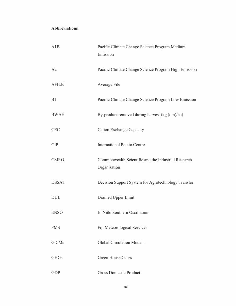
Abbreviations
A1B Pacific Climate Change Science Program Medium
Emission
A2 Pacific Climate Change Science Program High Emission
AFILE
Average File
B1 Pacific Climate Change Science Program Low Emission
BWAH By-product removed during harvest (kg (dm)/ha)
CEC Cation Exchange Capacity
CIP International Potato Centre
CSIRO
Commonwealth Scientific and the Industrial Research
Organisation
DSSAT Decision Support System for Agrotechnology Transfer
DUL Drained Upper Limit
ENSO El Niño Southern Oscillation
FMS Fiji Meteorological Services
G CMs Global Circulation Models
GHGs
Green House Gases
GDP Gross Domestic Product

xxiii
G2 Leaf Expansion Rate ( cm2/m2/d)
G3 Tuber Growth Rate (g/m2/d)
IBSNAT The International Benchmark Sites Network for
Agrotechnology Transfer
IPCC International Panel on Climate Change
LAI Leaf Area Index
LL Lower Limit
NAO Northern Atlantic Oscillation
NASA National Aeronautics and Space Administration
PACE-SD Pacific Centre for Environment and Sustainable
Development
PAR Photosynthetically Active Radiation
PCCSP Pacific Climate Change Science Program
PD Determinancy
PDO Pacific Decadal Oscillation
pH Percentage Hydrogen
PICs Pacific Island Countries
xxiv
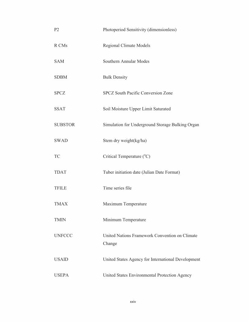
P2 Photoperiod Sensitivity (dimensionless)
R CMs Regional Climate Models
SAM Southern Annular Modes
SDBM Bulk Density
SPCZ SPCZ South Pacific Conversion Zone
SSAT Soil Moisture Upper Limit Saturated
SUBSTOR Simulation for Underground Storage Bulking Organ
SWAD Stem dry weight(kg/ha)
TC Critical Temperature (oC)
TDAT Tuber initiation date (Julian Date Format)
TFILE Time series file
TMAX Maximum Temperature
TMIN Minimum Temperature
UNFCCC United Nations Framework Convention on Climate
Change
USAID United States Agency for International Development
USEPA United States Environmental Protection Agency

xxv
UWAD Tuber dry weight (kg/ha)
UYAD Tuber fresh weight (t/ha)
UWAH Tuber dry weight (kg/ha)
UYAH Tuber fresh weight (t/ha)
xxvi
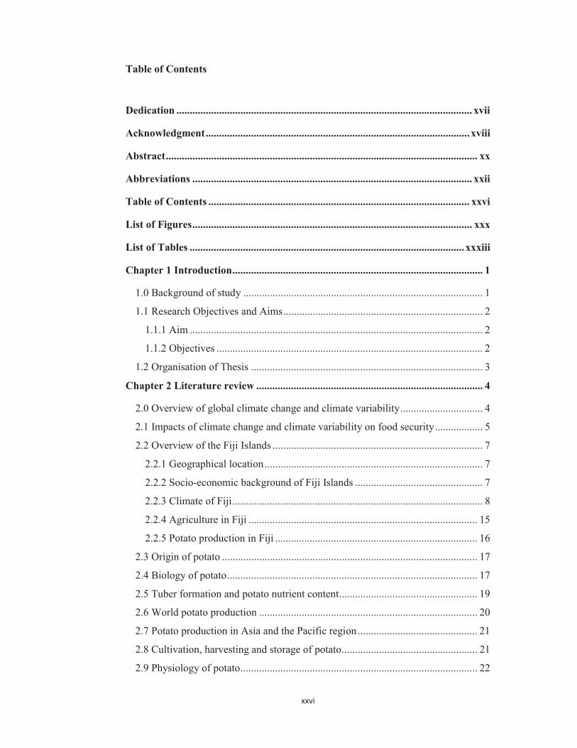
Table of Contents
Dedication ............................................................................................................... xvii
Acknowledgment ................................................................................................... xviii
Abstract ..................................................................................................................... xx
Abbreviations ......................................................................................................... xxii
Table of Contents .................................................................................................. xxvi
List of Figures ......................................................................................................... xxx
List of Tables ....................................................................................................... xxxiii
Chapter 1 Introduction .............................................................................................. 1
1.0 Background of study .......................................................................................... 1
1.1 Research Objectives and Aims ........................................................................... 2
1.1.1 Aim .............................................................................................................. 2
1.1.2 Objectives .................................................................................................... 2
1.2 Organisation of Thesis ....................................................................................... 3
Chapter 2 Literature review ..................................................................................... 4
2.0 Overview of global climate change and climate variability ............................... 4
2.1 Impacts of climate change and climate variability on food security .................. 5
2.2 Overview of the Fiji Islands ............................................................................... 7
2.2.1 Geographical location .................................................................................. 7
2.2.2 Socio-economic background of Fiji Islands ................................................ 7
2.2.3 Climate of Fiji .............................................................................................. 8
2.2.4 Agriculture in Fiji ...................................................................................... 15
2.2.5 Potato production in Fiji ............................................................................ 16
2.3 Origin of potato ................................................................................................ 17
2.4 Biology of potato .............................................................................................. 17
2.5 Tuber formation and potato nutrient content .................................................... 19
2.6 World potato production .................................................................................. 20
2.7 Potato production in Asia and the Pacific region ............................................. 21
2.8 Cultivation, harvesting and storage of potato. .................................................. 21
2.9 Physiology of potato ......................................................................................... 22

xxvii
2.10 Climate model system in prediction of agriculture and crop growth ............. 24
2.11 Implication of study ....................................................................................... 28
Chapter 3 Calibration of DSSAT SUBSTOR Potato Model ................................ 29
3.0 DSSAT overview ............................................................................................. 29
3.1 Methodology .................................................................................................... 30
3.1.1 Experimental site ....................................................................................... 30
3.1.2 Climate trends of field site ......................................................................... 31
3.1.3 Reason for site selection ............................................................................ 31
3.1.4 Data collection, treatments and importations ............................................ 31
3.1.5 Rainfed and nitrogen response experiment................................................ 37
3.1.6 DSSAT SUBSTOR Potato model calibration ........................................... 38
3.1.7 Genetic co-efficient adjustments ............................................................... 39
3.1.8 Analysis and outputs .................................................................................. 40
3.2 Results .............................................................................................................. 40
3.2.1 Soil information and water content recalculation ...................................... 41
3.2.2 Weather information .................................................................................. 42
3.2.3 Experimental file ....................................................................................... 44
3.2.4 Calibration ................................................................................................. 45
3.3 Discussion ........................................................................................................ 51
3.4 Recommendation .............................................................................................. 57
3.5 Experiment limitation ....................................................................................... 57
Chapter 4 Simulation of Desiree potato variety growth and yield in three
different sites (Banisogosogo, Koronivia and Nacocolevu) in Fiji using the
calibrated DSSAT SUBSTOR Potato Model ......................................................... 59
4.0 Introduction ...................................................................................................... 59
4.1 Methodology .................................................................................................... 61
4.1.1 Simulation sites .......................................................................................... 61
4.1.2 Reason for site selection ............................................................................ 62
4.1.3 Data collection, treatments and importations ............................................ 63
4.1.3 Model simulation under current climatic and potential conditions ........... 63
4.1.4 Optimisation treatment through sensitivity analysis.................................. 65
4.1.5 Climate variability (El Niño Southern Oscillation) ................................... 66
4.1.6 Data analysis .............................................................................................. 67

xxviii
4.2 Results .............................................................................................................. 67
4.2.1 Weather data .............................................................................................. 67
4.2.2 Simulation results for Desiree ................................................................... 69
4.2.3 Optimisation treatments ............................................................................. 77
4.2.4 Climate variability (El Niño Southern Oscillation) simulation ................. 81
4.3 Discussion ........................................................................................................ 85
4.3.1 Desiree potential simulation ...................................................................... 85
4.3.2 Desiree non-potential simulation ............................................................... 85
4.3.3 Optimisation treatments ............................................................................. 90
4.3.4 ENSO effect ............................................................................................... 94
4.4 Recommendations ............................................................................................ 95
4.5 Challenges faced .............................................................................................. 98
Chapter 5 Simulating the impacts of future climatic scenario on potato
production in Fiji using the calibrated DSSAT SUBSTOR Potato model ......... 99
5.0 Introduction ...................................................................................................... 99
5.1 Methodology .................................................................................................. 102
5.1.1 Simulation sites ........................................................................................ 102
5.1.2 Data collection, treatments and importations .......................................... 102
5.1.3 Optimisation treatments ........................................................................... 103
5.1.4 Model output analysis .............................................................................. 103
5.2 Results ............................................................................................................ 103
5.2.1 Future climate simulations ....................................................................... 104
5.2.2 Optimisation treatments ........................................................................... 113
5.3 Discussion ...................................................................................................... 116
5.3.1 Potential simulations ................................................................................ 116
5.3.2 Non-potential simulations ........................................................................ 119
5.3.3 Optimisation treatments ........................................................................... 124
5.4 Recommendations .......................................................................................... 129
5.5 Research limitations ....................................................................................... 130
Chapter 6 Simulating the performance of potential potato varieties under
current and future climates in Banisogosogo, Fiji Islands. ................................ 132
6.0 Introduction .................................................................................................... 132
6.1 Methodology .................................................................................................. 133
xxix
6.1.1 Model simulation under current climate .................................................. 133
6.1.2 Model simulation under future climatic conditions ................................. 134
6.1.3 Model output analysis .............................................................................. 134
6.2 Results ............................................................................................................ 135
6.2.1 Current climate simulations ..................................................................... 135
6.2.2 Optimisation treatments ........................................................................... 141
6.2.3 Climate variability (El Niño Southern Oscillation) simulation ............... 144
6.2.2 Future climate simulations ....................................................................... 147
6.3 Discussion ...................................................................................................... 154
6.3.1 Current climate simulations ..................................................................... 154
6.3.2 Future climate simulation ........................................................................ 159
6.4 Recommendations .......................................................................................... 166
6.4.1 Current climate simulation ...................................................................... 166
6.4.2 Future climate simulation for Sebago variety .......................................... 166
6.4.2 Future climate simulation for Russet Burbank variety ............................ 167
6.5 Research limitations ....................................................................................... 167
Conclusion .............................................................................................................. 168
Bibliography ........................................................................................................... 171
Appendices .............................................................................................................. 198
Appendix 1: Calibration ....................................................................................... 198
Appendix 2: Current climate simulations ............................................................. 201
Appendix 3: Future climate simulations .............................................................. 213
Appendix 4: Simulation of other potato varieties ................................................ 260

xxx
List of Figures
Figure 2.0 shows Fiji’s location in the Pacific…………………………… 8
Figure 2.1 shows the number of cyclones passing within 400km of
Suva…………………………………………………………………………
10
Figure 2.2 shows the southern oscillation graph…………………………… 11
Figure 2.3 shows the South Pacific Convergence Zone and Intertropical
Convergence Zone…………………………………………………………..
11
Figure 2.4 shows the mean annual temperatures and rainfall for Suva and
Nadi………………………………………………………………………….
12
Figure 2.5 shows the atmospheric concentration of atmospheric carbon
dioxide for all three emission scenarios……………………………………..
14
Figure 2.6 shows the transfer and spread of potatoes……………………… 17
Figure 3.0 shows the location of experimental site (Banisogosogo)………. 30
Figure 3.1 showing collection of sample soil and marking
of replicate plot ……………………………………………………………
33
Figure 3.2 shows the design of the experimental replicate plot……………. 34
Figure 3.3 shows tuber initiation during T1……………………………… 35
Figure 3.4 shows measurement of LAI using AccuPAR
LP-80 and tubers during T2……………………………………................
35
Figure 3.5 shows tubers at T2 and pest infections………………………. 35
Figure 3.6 shows nematode infection , beetle infection
(Papuana spp.) and pest Quantula striata………………………………..
36
Figure 3.7 shows tubers during final harvest………………………………. 36
Figure 3.8 shows the daily rainfall for Banisogosogo from
January to September, 2012…………………………………………………
43
Figure 3.9 shows the daily maximum and minimum temperature for
Banisogosogo from January to September, 2012………………………….
44
Figure 3.10 shows the simulated and observed for Desiree
before calibration……………………………………………………………
47
Figure 3.11 shows the potential and observed calibration results for
Desiree ………………………………………………………………
49
Figure 3.12 shows the evaluation of potato yield (dry matter in kg/ha) at
Banisogosogo Fiji for year 2012…………………………………………….
50
Figure 4.0 shows the location of three simulation sites……………………. 62

xxxi
Figure 4.1 shows the monthly average rainfall for Banisogosogo,
Koronivia and Nacocolevu…………………………………………………..
68
Figure 4.2 shows the monthly average maximum and minimum
temperature for Banisogosogo, Koronivia and Nacocolevu……………….
68
Figure 4.3 shows Banisogosogo potential and non-potential simulations
for stem weight, LAI, tuber fresh weight, leaf weight, tops weight and
tuber dry weight……………………………………………………………..
71
Figure 4.4 shows Koronivia potential and non-potential simulations for
LAI, leaf weight, stem weight, tuber fresh weight, tuber dry weight and
tops weight…………………………………………………………………..
72
Figure 4.5 shows Nacocolevu potential and non-potential simulations for
LAI, leaf weight, stem weight, tuber fresh weight, tuber dry weight and
tops weight…………………………………………………………………..
73
Figure 4.6 shows the impact of precipitation, total water and nitrogen
content in soil on non-potential tuber dry yield and LAI for Desiree in
Banisogosogo over the growing season………………………………….
74
Figure 4.7 shows the impact of precipitation, total water and nitrogen
content in soil on non-potential tuber dry yield and LAI for Desiree in
Koronivia over the growing season………………………………………
75
Figure 4.8 shows the impact of precipitation, total water and nitrogen
content in soil on non-potential tuber dry yield and LAI for Desiree in
Nacocolevu over the growing season……………………………………
76
Figure 5.0 shows the potential future climate simulations for
Banisogosogo for LAI, leaf weight, stem weight, tuber fresh weight, tops
weight, tuber dry weight and tuber fresh weight……………………………
107
Figure 5.1 shows the non-potential future climate simulation for
Banisogosogo under A1B and A2 emission scenario for LAI, leaf weight,
stem weight, tuber fresh weight, tuber dry weight and tops weight………..
108
Figure 5.2 shows the Koronivia potential future climate simulations for
LAI, leaf weight, stem weight, tuber fresh weight, tuber dry weight and
tops weight…………………………………………………………………..
109
Figure 5.3 shows the Koronivia non-potential future climate simulations
for LAI, leaf weight, stem weight, tuber fresh weight, tuber dry weight and
xxxii
tops weight…………………………………………………………………. 110
Figure 5.4 shows the Nacocolevu potential future climate simulations for
LAI, leaf weight, stem weight, tuber fresh weight, tuber dry weight and
tops weight…………………………………………………………………
111
Figure 5.5 shows the Nacocolevu non-potential future climate simulation
for LAI, leaf weight, stem weight, tuber fresh weight, tuber dry weight and
tops weight…………………………………………………………………..
112
Figure 6.0 shows Banisogosogo potential and non-potential simulations
for Sebago for LAI, leaf weight, stem weight, tuber dry and fresh weight
and tops weight……………………………………………………………...
137
Figure 6.1 shows the Banisogosogo potential and non-potential
simulations for Russet Burbank for LAI, leaf weight, stem weight, tuber
dry and fresh weight and tops weight……………………………………….
138
Figure 6.2 shows the impact of precipitation, total water and nitrogen
content in soil on non-potential tuber dry yield and LAI for Sebago in
Banisogosogo over the growing season…………………………………….
139
Figure 6.3 shows the impact of precipitation, total water and nitrogen
content in soil on non-potential tuber dry yield and LAI for Russet Burbank
in Banisogosogo over the growing season…………………………………..
140
Figure 6.4 shows Banisogosogo future climate potential simulations for
Sebago for LAI, leaf weight, stem weight, tuber dry and fresh weight and
tops weight…………………………………………………………………..
148
Figure 6.5 shows Banisogosogo future climate non-potential simulations
for Sebago for LAI, leaf weight, stem weight, tuber dry and fresh weight
and tops weight……………………………………………………………...
149
Figure 6.6 shows Banisogosogo future climate potential simulations for
Russet Burbank for LAI, leaf weight, stem weight, tops weight, tuber fresh
and tuber dry weight under A1B and A2 emission scenario………………..
152
Figure 6.7 shows Banisogosogo future climate non potential simulations
for Russet Burbank for LAI, leaf weight, stem weight, tops weight, tuber
fresh and tuber dry weight under A1B and A2 emission scenario…………
153

xxxiii
List of Tables
Table 2.0 Shows the climate trends in Fiji from 1961- 2010………………. 13
Table 2.1 shows the projected average annual air temperature change for
Fiji under low emission scenario (B1), medium emission scenario (A1B)
and high emission scenario (B2) ……………………………………………
15
Table 2.2 shows the taxonomy of potato…………………………………… 18
Table 3.0 shows the planting information………………………………….. 39
Table 3.1 shows the DSSAT SUBSTOR Potato model input and data
requirement.………………............................................................................
40
Table 3.2 shows the chemical properties of Banisogosogo soil for each
replicate plot…………………………………………………………………
41
Table 3.3 shows the physical properties of Banisogosogo soil for each
replicate plot…………………………………………………………………
42
Table 3.4 shows the recalculated water content of bulk density, lower limit
of extractable soil water, drained upper limit and saturation for
Banisogosogo soil…………………………………………………………..
42
Table 3.5 shows Banisogosogo monthly average weather data…………… 43
Table 3.6 shows the values for AFile (Average File)……………………… 44
Table 3.7 shows the values for Time Series file (Tfile)…………………… 45
Table 3.8 shows the simulation results for Desiree before calibration…….. 46
Table 3.9 shows the recalibration of genetics co-efficient………………… 48
Table 3.10 shows the simulation results after calibration
for Desiree ………………………………………………………………….
48
Table 4.0 shows the summary of simulations at Banisogosogo, Koronivia
and Nacocolevu……………………………………………………………...
64
Table 4.1 shows the irrigation application during simulations at
Banisogosogo, Koronivia and Nacocolevu………………………………….
65
Table 4.2 shows the fertiliser application during simulations at
Banisogosogo, Koronivia and Nacocolevu…………………………………
65
Table 4.3 shows the average monthly maximum temperature, minimum
temperature and rainfall for Banisogosogo, Koronivia and Nacocolevu….
69

xvii
Table 4.4 shows the potential (non-limiting for water and nitrogen) and non-
potential (limiting for water and nitrogen) simulation results of current climate
for Banisogosogo, Koronivia and Nacocolevu………………………...
70
Table 4.5 shows the yield at different planting time for Banisogosogo,
Koronivia and Nacocolevu……………………………………………………..
77
Table 4.6 shows the yield at different row spacing……………………………. 78
Table 4.7 shows the yield under different irrigation application and irrigation
amount…………………………………………………………………………...
78
Table 4.8 shows the planting depth with corresponding yield………………… 79
Table 4.9 shows the application of fertiliser (banded beneath surface) and
corresponding yield for Banisogosogo using weather data of 2012……………
79
Table 4.10 shows the optimum fertiliser and irrigation management simulation
for Banisogosogo using weather data of 2012………………………………….
80
Table 4.11 shows the application of fertiliser (banded beneath surface) and
corresponding yield for Koronivia using weather data of 2010.……………….
80
Table 4.12 shows the corresponding yield of optimum fertiliser and irrigation
management for Koronivia using weather data of 2010………………………..
80
Table 4.13 shows the application of fertiliser (banded beneath surface) and
corresponding yield for Nacocolevu using weather data of 2010………………
81
Table 4.14 shows the corresponding yield of optimum fertiliser and irrigation
management for Nacocolevu using weather data of 2010………………………
81
Table 4.15 shows the impact of ENSO on potato yield for non-potential
Banisogosogo simulation from 1983-2012……………………………………...
82
Table 4.16 shows the 7 year average for ENSO yield for Banisogosogo……… 82
Table 4.17 shows the impact of ENSO on potato yield for non-potential
Koronivia simulation from 1990 to 2010……………………………………….
83
Table 4.18 shows the 5 Year average for ENSO yield for Koronivia………….. 83
Table 4.19 shows the impact of ENSO on potato yield for non-potential
Nacocolevu simulation from 1990-2010………………………………………..
84
Table 4.20 shows the 5 Year average for ENSO yield for Nacocolevu………. 84
Table 5.0 shows the environment modification climatic parameters…………... 102
Table 5.1 shows the Banisogosogo simulation results of future climate
simulation………………………………………………………………………..
104

xviii
Table 5.2 shows the Koronivia simulation results of future
climate simulation……………………………………………………….............
105
Table 5.3 shows Nacocolevu simulation results of future climate
simulation……………………………………………………………………….
105
Table 5.4 shows the optimisation treatments at Banisogosogo..……………… 113
Table 5.5 shows the optimisation treatments at Koronivia…………………….. 114
Table 5.6 shows the optimisation treatments at Nacocolevu…………………… 115
Table 6.0 shows the genetic co-efficient of Sebago and
Russet Burbank………………………………………………………………….
133
Table 6.1 Shows Sebago, Russet Burbank and Desiree potential
and non-potential simulation under current climate simulations for
Banisogosogo……………………………………………………………………
135
Table 6.2 shows the yield at different planting time for Banisogosogo……… 141
Table 6.3 shows the yield at different row spacing for Banisogosogo………. 142
Table 6.4 shows the yield under different irrigation application and irrigation
amount for Banisogosogo……………………..................................................
142
Table 6.5 shows the planting depth with corresponding yield for
Banisogosogo……………………………………………………………………
143
Table 6.6 shows the application of fertiliser (banded beneath surface) and
corresponding yield for Banisogosogo for Sebago variety………………….....
143
Table 6.7 shows the optimum fertiliser and irrigation management for
Banisogosogo for Sebago variety…………………………………………….....
143
Table 6.8 shows the application of fertiliser (banded beneath surface) and
corresponding yield for Banisogosogo for Russet Burbank……………………
144
Table 6.9 shows the optimum fertiliser and irrigation management for
Banisogosogo for Russet Burbank………………………………………………
144
Table 6.10 shows the impact of ENSO on potato yield for Sebago variety at
Banisogosogo from 1983-2012………………………………………………….
145
Table 6.11 shows the 7 year average for ENSO yield for Banisogosogo for
Sebago variety. The highest yield was obtained by the neutral
years……………………………………………………………………………..
146
Table 6.12 shows the impact of ENSO on potato yield for Banisogosogo for
Russet Burbank from 1983-2010……………………………………………….
146
xix
Table 6.13 shows 7 year average for ENSO yield for Banisogosogo for Russet
Burbank. The highest yield was obtained under neutral
year………………………………………………………………………………
147
Table 6.14 shows the Banisogosogo future climate simulation for Sebago
variety……………………………………………………………………………
147
Table 6.15 shows the optimisation treatments for Sebago…………………….. 151
Table 6.16 shows Banisogosogo simulation results of future climate simulation
for Russet Burbank Variety for A1B and A2 emission
scenario…………………………………………………………………………..
151
Table 6.17 shows the optimisation treatments for Russet Burbank…………… 154

1
Chapter 1 Introduction
1.0 Background of study
Potato was first introduced in Fiji by European settlers in 1860’s and since then the
consumption of potatoes has increased. Potato has been cultivated in Fiji for many
years but only on a small scale. Only recently (1960’s onwards), potato was given a
priority in research programmes. Since then, potato trials have been conducted in
Sigatoka Valley, Nadi, Ba and Nadarivatu to investigate suitable cultivar, row
spacing, plant growth and yield, disease tolerance including intercropping. Tests
were conducted to identify suitable varieties for cultivation in Fiji in collaboration
work with the International Potato Centre (CIP) in the 1980’s. Research has also
been conducted on better ways of producing and making accessible seed including
vegetative planting resources for farmers by numerous scientists over the decades in
Fiji (Autar, 2009). Currently, Fiji imports around 16 000 tonnes of potatoes annually
valued at $17 million. Under its Import Substitution programme, the government of
Fiji aims to reduce its potato imports and boost local food production (Mudaliar,
2007; Fiji Times Online, 2010; The Fijian Government, 2010).
This study was set out to evaluate the impacts of climate change and climate
variability on potato production in Fiji and to help identify strategies to optimise
potato yield and identify which varieties of potato can perform better under current
and future climatic conditions of Fiji. Many Pacific Island Countries (PICs) are
among the first to suffer the impacts of climate change. Subsistence and commercial
agriculture are being adversely affected by climate change in PICs (Asian
Development Bank, 2009; Wairiu et al., 2012). Some of the challenges to agriculture
and crop production in PICs include: lack of consideration of climate change in
current development strategies and activities (Quity, 2012). There is also low level of
awareness on climate change, inadequate capacity at community, national and
regional level to develop and implement adaptation strategies. Not only these, but
limited resources and inaccessibility on reliable data on climate change impact on the
region and as well as the lack of resource allocation in agricultural sector are also
some of the challenges faced by the agricultural sector (Wairiu et al., 2012).

2
The motivation for this study arose when I was given an assignment to develop a
research proposal with the theme of climate change and sustainable development.
With the knowledge that food security is an important issue for climate change, I
began to research on the impacts of climate change on staple crops. Coincidently,
potato was being reintroduced to Fiji during that time. However, the fate of potato
industry remained uncertain. Therefore, I decided to look into crop modeling which
not only helps to predict the behavior of the biological system but can also be used
for agronomic efficiency and to promote environmental management. At the same
time, the crop model software Decision Support System for Agrotechnology Transfer
(DSSAT) v4.5 was introduced in Pacific Centre for Environment and Sustainable
Development (PACE-SD) for the students to utilise for research projects. It is hoped
that this research will assist the agricultural sector to improve the yield of potatoes
and to support farmer’s livelihood and to provide food security for Fiji using modern
technology.
1.1 Research Objectives and Aims
1.1.1 Aim
This study investigates how climate change and climate variability affects potato
production in Fiji.
1.1.2 Objectives
The objectives of this study are to:
� calibrate the DSSAT SUBSTOR Potato Model’s performance in
Banisogosogo, Fiji using Desiree variety.
� simulate potato production under current climatic condition and optimise crop
management to maximise potato yield under current conditions.
� simulate potato production under future climatic scenario and to optimise
crop management strategies to maximise potato yield under stressful
conditions.
� identify other potato varieties that may perform better under Fiji’s current and
future conditions using simulation approach.

3
1.2 Organisation of Thesis
This thesis is divided into six chapters. Chapter 1 provides background information
and states the aims and research objectives. Chapter 2 is a literature review and sets
the context of how climate change and climate variability affects food security,
overview of Fiji Islands and potato production in Fiji. It also gives information on
origin, history, distribution and cultivation of potatoes, the use of climate model
systems in prediction of agriculture and crop growth and implication of study.
Chapter 3 calibrates the DSSAT SUBSTOR Potato model in Banisogosogo Fiji using
Desiree variety. Chapter 4 discusses how current climate and climate variability has
had an impact on potato production in Banisogosogo, Koronivia and Nacocolevu and
what strategies are used to maximise potato yield. Chapter 5 describes how future
climate change (Pacific Climate Change Science Program emission scenario for
medium emission (A1B) and high emission (B2) for 2030, 2055 and 2090) will
affect potato production in Banisogosogo, Koronivia and Nacocolevu and what could
be some of the strategies to maximise potato yield. Finally, Chapter 6 states which
cultivar can perform better in Fiji’s current and future climate conditions.

4
Chapter 2 Literature review
2.0 Overview of global climate change and climate variability
According to the United Nations Framework Convention on Climate Change
(UNFCCC), climate change is defined as a “change in the climate which is attributed
directly or indirectly to human activity that alters the composition of global
atmosphere and which is in additional to natural climate variability observed over
comparable time periods” (Intergovernmental Panel on Climate Change, 2001;
United Nations Framework Convention on Climate Change, 2012). Climate
variability is defined as “variation in the mean state and other statistics (such as
standard deviation, the occurrence of extremes) of the climate on all temporal and
spatial scales beyond that of individual weather events over a period of time, for
example, month, season or a year” (Intergovernmental Panel on Climate Change,
2001; World Meteorological Organisation, 2003).
The Intergovernmental Panel on Climate Change (IPCC), in its Climate Change
2007: Synthesis Report, stated that “warming of the climate system is unequivocal,
as is now evident from observations of increases in global average air and ocean,
widespread melting of snow and ice and rising global average sea level”. The IPCC
has acknowledged changes in atmospheric concentration of greenhouse gases
(GHGs), land cover and solar radiation to alter the energy balance of the climate
system and act as the key drivers of climate change (Intergovernmental Panel on
Climate Change, 2007a). The global concentrations of greenhouse gases (GHGs),
such as, carbon dioxide, methane and nitrous dioxide has increased noticeably owing
to anthropogenic causes since 1750’s and now far exceed the pre-industrial values.
The global atmospheric concentration of carbon dioxide has increased from 280 ppm
from pre-industrial times to 379 ppm in 2005 which surpasses by far the natural
range over the last 650, 000 years as determined for ice-cores. The primary reasons
for the global increase in the atmospheric concentration of carbon dioxide are due to
changes in fossil fuel usage and changes in land use patterns whereas the reason for
increase in the concentrations of methane and nitrous oxide is due to agriculture.
Since 1850, eleven of the last twelve years (1995-2006), rank amongst the twelve
warmest years on record. Evidence also exists for the changes in global circulation,
for example, the poleward shift and strengthening of the westerly winds and
noticeable changes in ocean biogeochemistry and salinity. Precipitation events will
5
also be strengthened in a warmer world, with the extensive increase in heavy
precipitation events and increased likelihood of flooding. Warming is also consistent
with sea-level rise. The global average sea level rose at an average rate of 1.8 mm
[1.3 to 2.3 mm] per year over 1961-2003 (Intergovernmental Panel on Climate
Change, 2007b). North Atlantic has noted fluctuations in westerlies and storm track
and these are fluctuations are described by the Northern Atlantic Oscillation (NAO).
In the Southern Hemisphere, due to robust warming over the Antarctic Peninsula
and, to a lesser extent, cooling over the continental parts of Antarctica, there has been
a change in circulation related to an increase in Southern Annular Modes (SAM)
from 1960s to the present (Solomon et al., 2007).
In the Pacific, changes have also been noticed in the ocean-atmosphere interactions.
On interannual time scales, El Niño Southern Oscillation (ENSO) is the dominant
form of global-scale variability. The shift in climate in 1976-1977, is related to the
phase change in Pacific Decadal Oscillation (PDO). This brought about more El
Niño events and variations in the evolution of ENSO, which affected many areas.
Over the 20th century, the Pacific has experienced considerable low frequency
atmospheric variability, with extended periods of weakened circulations (1900-1924,
1947-1976) also periods of strengthened circulations (1925-1946, 1977-2005).
Interannual variability, such as ENSO and North Atlantic Oscillation (NAO), can
also be related to regional average sea level rise (Solomon et al., 2007). Models also
indicate that there is a tendency for more warming in the central and east Pacific than
in the west. Although this east west difference in warming is usually less than a
degree in multi-model ensemble (Boer et al., 2001).
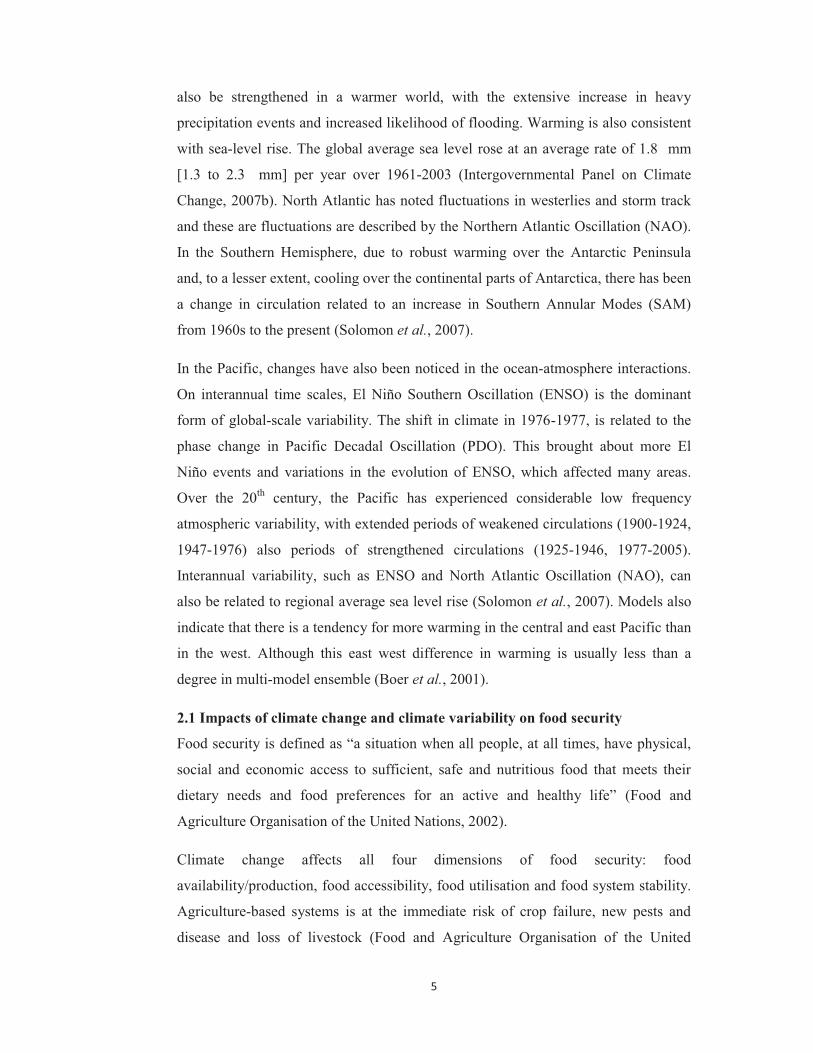
2.1 Impacts of climate change and climate variability on food security
Food security is defined as “a situation when all people, at all times, have physical,
social and economic access to sufficient, safe and nutritious food that meets their
dietary needs and food preferences for an active and healthy life” (Food and
Agriculture Organisation of the United Nations, 2002).
Climate change affects all four dimensions of food security: food
availability/production, food accessibility, food utilisation and food system stability.
Agriculture-based systems is at the immediate risk of crop failure, new pests and
disease and loss of livestock (Food and Agriculture Organisation of the United

6
Nations, 2008a). The rise in global mean average temperature will have an impact on
agronomic productions, such as, changes in growing seasons. Sea level rise will
diminish the quantity of land accessible for agriculture (Darwin, 2001). Due to
climate change agriculture has to compete with other sectors for land, water and also
investment of time and money (Schi mmelpfennig et al., 1996). In developing
countries, almost 11% of arable land be could be affected by climate change (Food
and Agriculture Organisation of the United Nations, 2007). Climate change impacts
can be divided into two impact categories: biophysical impacts and socio-economic
impacts. Biophysical impacts include: physiological effects on crops, pasture, forests
and livestock, changes in the quality and quantity of land, soil and water resources,
increased weed and pest challenges, changes in the spatial and temporal distribution
of impacts, rise in sea level, changes to ocean acidity, increased intensity and
frequency of storms, drought and flooding, altered hydrological cycles and changes
in precipitation have implication for future food availability (Food and Agriculture
Organisation of the United Nations, 2007). On the other hand, socio-economic
impacts consist of: decline in yields and production, reduced marginal GDP from
agriculture, fluctuation in world market prices, increase in the number of people at
risk at geographical distribution of trade regimes, migration and civil unrest (Food
and Agriculture Organisation of the United Nations, 2007). Due to multiple socio-
economic and bio-physical factors affecting food systems and food security, the
capacity for a food system to diminish its vulnerability to climate change is not
uniform as this will require better systems of food production, food distribution and
economic access for food systems to be able to manage with climate change. The key
to addressing these challenges can be conducted through developing a framework
system which deliberates all stresses to the food system such as social stress, political
stress and environmental stress and the communities can learn from past experience
of environmental stress, relevant past adaptation measures and indigenous
knowledge (Gregory et al., 2005).
Climatic variability will bring additional challenges (Gregory et al., 2005). Short
term rainfall variability can pose as a major risk factor. It can lead to soil moisture
deficits, crop damage and crop disease all related to distribution of rainfall and
associated humidity (Ludi, 2009).

7
2.2 Overview of the Fiji Islands
2.2.1 Geographical location
The Fiji Islands comprises of more than 330 islands and has an overall land area of
18 300 km2 and an Economic Exclusive Zone of 1.3 million km2. The geographical
co-ordinates of the Fiji Islands are between longitude 175oEast and 178oWest and
latitude 15o and 22oSouth. It is located about 2100 km north of Auckland, New
Zealand. The biggest island is Viti Levu (10 429 km2), which covers 57% of the total
land area and Vanua Levu which covers 5556 km2. The capital of Fiji is Suva with
the center of politics and economy in Fiji. Other main islands include Taveuni (470
km2), Kadavu (411 km2), Gau (140 km2) and Koro (104 km2) (Pacific Islands
Climate Change Assistance Programme and Fiji Country Team, 2005; Vanualailai
and UNFCCC Consultant, 2008; GEF et al., 2009; Australian Bureau of Meterology
and CSIRO, 2011). The geography of Fiji is dominated by mountainous terrain and
due to earthquakes and volcanic eruptions, the terrain of Fiji is somewhat rugged.
The highest point is Mount Tomanivi which is 1324m. The larger islands of Fiji,
such as Viti Levu and Vanua Levu, are as a result of volcanic activities of the past
whereas the smaller islands are made up of coral reefs. The flora and fauna of the
island is determined by the tropical climate of the islands (Maps of World, 2010,
2011).
2.2.2 Socio-economic background of Fiji Islands
Fiji became independent in 1970 after being a British Colony for nearly a century
(CIA World Factbook, 2012a). It is blessed with natural resources such as timber,
gold, copper, fish, offshore oil and hydro-power (Maps of World, 2010, 2011). The
Fijian population comprises several ethic groups such as Fijian, Indian descendents,
Chinese, European and others (Pacific Islands Climate Change Assistance
Programme and Fiji Country Team, 2005). From July 2011, the estimated population
of Fiji stands at 890, 057 (Index Mundi, 2012). In recent years, there has been an
increasing trend of urbanisation which has led to the development of major squatter
settlements around town areas (Pacific Islands Climate Change Assistance
Programme and Fiji Country Team, 2005). Fiji’s Gross Domestic Product (GDP) at
current basic price for 2010 was estimated to grow at 7.9%. This is an increase from
8.8% from 2009 when the growth rate was considered to be -0.9%. The Transport

8
Storage sector and the Communication sector were the largest contributors to the
growth in GDP which accounted for 15.6% of the GDP followed by Manufacturing
sector and Wholesale and Retail sector which contributed 15.0% and 11% of the
GDP respectively (Bureau of Statistics, 2011).
Figure 2.0 shows Fiji’s location in the Pacific. Source: (Maps of World, 2012)
2.2.3 Climate of Fiji
2.2.3.1 Current climate
The annual average temperature of Fiji is between 20oC-27oC. The variations in the
temperature from one season to another are relatively small and can strongly be
linked to changes in the surrounding ocean temperature. Between the coolest months
(July and August) and the warmest months (January to February), the average
temperature difference is only about 2°C-4°C (Fiji Meterological Services, 2012).
The mean night temperature of Fiji can be as low as 18oC (in the central parts of the
main islands, the temperatures can be as low as 15oC) whereas the maximum mean
day time temperatures can be as high as 32oC. Past records also indicate that extreme
temperatures as low as 8°C and as high as 39.4 °C have been documented in Fiji (Fiji
9
Meterological Services, 2012). The inter-annual variations in temperature are low,
generally ranging from ± 0.5 °C about the long term mean (Pacific Islands Climate
Change Assistance Programme and Fiji Country Team, 2005).
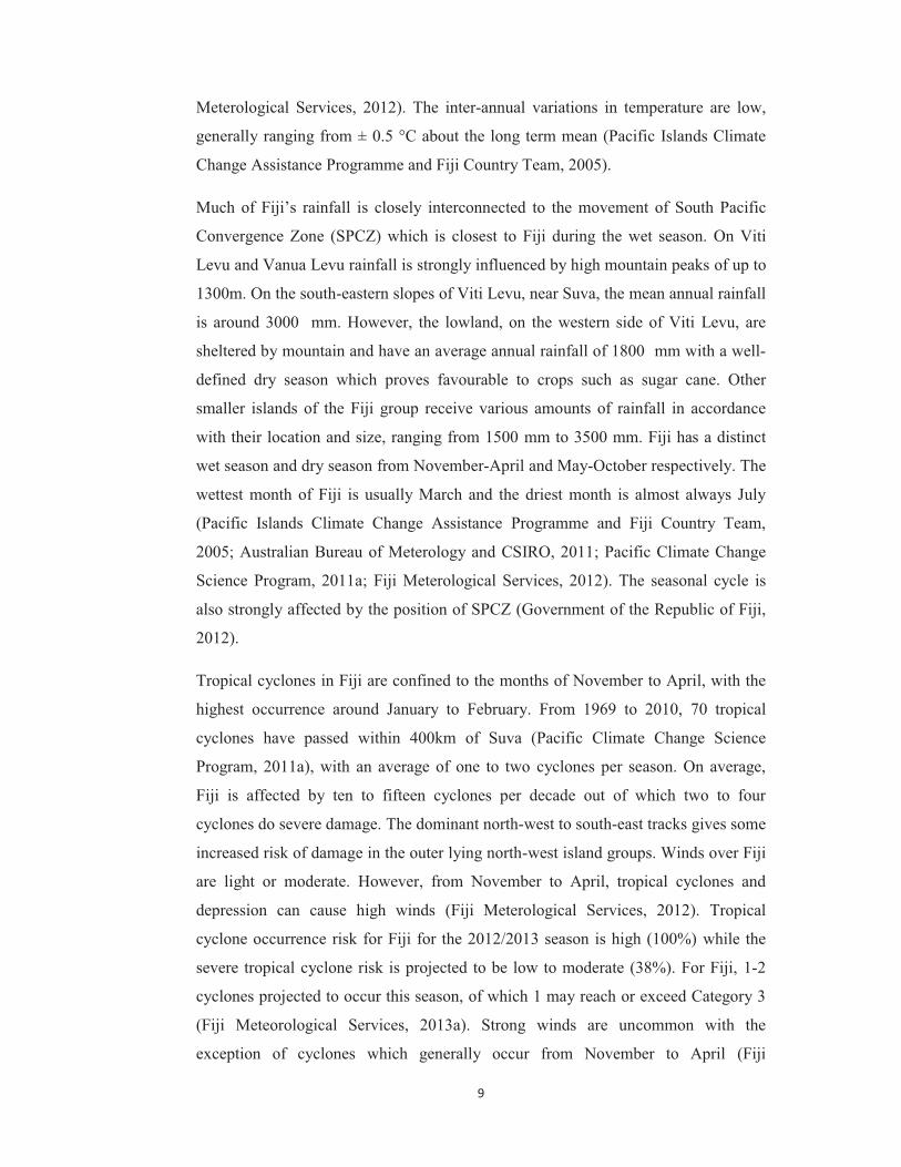
Much of Fiji’s rainfall is closely interconnected to the movement of South Pacific
Convergence Zone (SPCZ) which is closest to Fiji during the wet season. On Viti
Levu and Vanua Levu rainfall is strongly influenced by high mountain peaks of up to
1300m. On the south-eastern slopes of Viti Levu, near Suva, the mean annual rainfall
is around 3000 mm. However, the lowland, on the western side of Viti Levu, are
sheltered by mountain and have an average annual rainfall of 1800 mm with a well-
defined dry season which proves favourable to crops such as sugar cane. Other
smaller islands of the Fiji group receive various amounts of rainfall in accordance
with their location and size, ranging from 1500 mm to 3500 mm. Fiji has a distinct
wet season and dry season from November-April and May-October respectively. The
wettest month of Fiji is usually March and the driest month is almost always July
(Pacific Islands Climate Change Assistance Programme and Fiji Country Team,
2005; Australian Bureau of Meterology and CSIRO, 2011; Pacific Climate Change
Science Program, 2011a; Fiji Meterological Services, 2012). The seasonal cycle is
also strongly affected by the position of SPCZ (Government of the Republic of Fiji,
2012).
Tropical cyclones in Fiji are confined to the months of November to April, with the
highest occurrence around January to February. From 1969 to 2010, 70 tropical
cyclones have passed within 400km of Suva (Pacific Climate Change Science
Program, 2011a), with an average of one to two cyclones per season. On average,
Fiji is affected by ten to fifteen cyclones per decade out of which two to four
cyclones do severe damage. The dominant north-west to south-east tracks gives some
increased risk of damage in the outer lying north-west island groups. Winds over Fiji
are light or moderate. However, from November to April, tropical cyclones and
depression can cause high winds (Fiji Meterological Services, 2012). Tropical
cyclone occurrence risk for Fiji for the 2012/2013 season is high (100%) while the
severe tropical cyclone risk is projected to be low to moderate (38%). For Fiji, 1-2
cyclones projected to occur this season, of which 1 may reach or exceed Category 3
(Fiji Meteorological Services, 2013a). Strong winds are uncommon with the
exception of cyclones which generally occur from November to April (Fiji
10
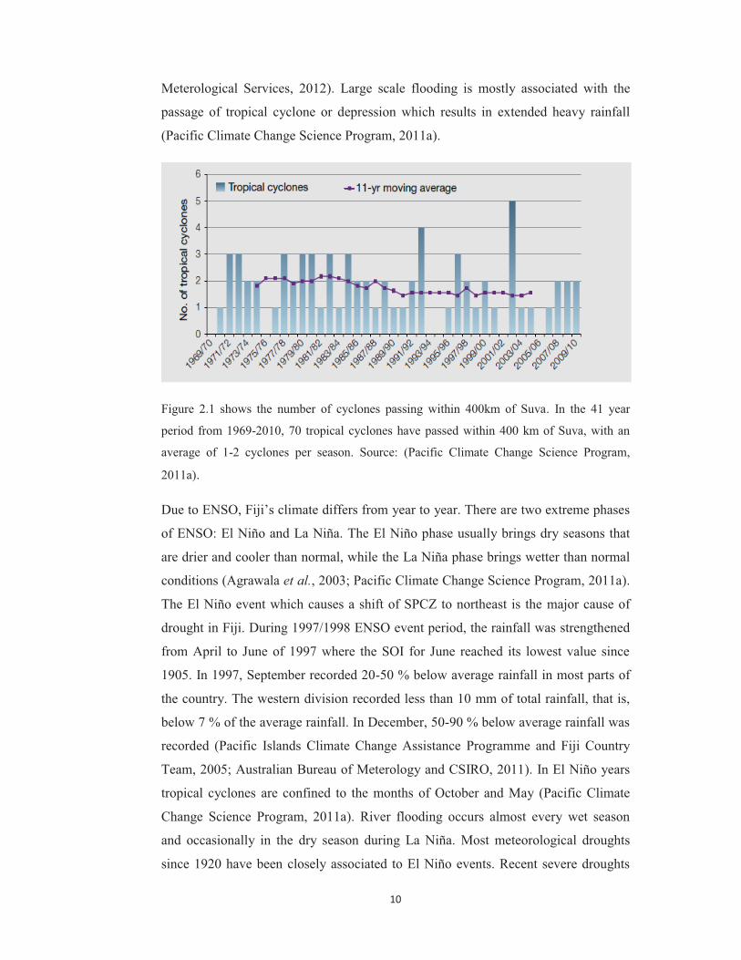
Meterological Services, 2012). Large scale flooding is mostly associated with the
passage of tropical cyclone or depression which results in extended heavy rainfall
(Pacific Climate Change Science Program, 2011a).
Figure 2.1 shows the number of cyclones passing within 400km of Suva. In the 41 year
period from 1969-2010, 70 tropical cyclones have passed within 400 km of Suva, with an
average of 1-2 cyclones per season. Source: (Pacific Climate Change Science Program,
2011a).
Due to ENSO, Fiji’s climate differs from year to year. There are two extreme phases
of ENSO: El Niño and La Niña. The El Niño phase usually brings dry seasons that
are drier and cooler than normal, while the La Niña phase brings wetter than normal
conditions (Agrawala et al., 2003; Pacific Climate Change Science Program, 2011a).
The El Niño event which causes a shift of SPCZ to northeast is the major cause of
drought in Fiji. During 1997/1998 ENSO event period, the rainfall was strengthened
from April to June of 1997 where the SOI for June reached its lowest value since
1905. In 1997, September recorded 20-50 % below average rainfall in most parts of
the country. The western division recorded less than 10 mm of total rainfall, that is,
below 7 % of the average rainfall. In December, 50-90 % below average rainfall was
recorded (Pacific Islands Climate Change Assistance Programme and Fiji Country
Team, 2005; Australian Bureau of Meterology and CSIRO, 2011). In El Niño years
tropical cyclones are confined to the months of October and May (Pacific Climate
Change Science Program, 2011a). River flooding occurs almost every wet season
and occasionally in the dry season during La Niña. Most meteorological droughts
since 1920 have been closely associated to El Niño events. Recent severe droughts

11
have occurred in 1987, 1992, 1997-98, 2003 and 2010 (Pacific Climate Change
Science Program, 2011a).
Figure 2.2 shows the southern oscillation graph. The SOI is shown in bars while the 5 month
running mean is shown in continuous pink line. The figure shows that SOI has risen from -
3.6 in February to +11.1 in March. Source: (Fiji Meteorological Services, 2013b).
Figure 2.3 shows the South Pacific Convergence Zone and Intertropical Convergence Zone.
The arrow indicates near surface winds while the blue shading represents the band of rainfall
convergence zone, the red dashed oval represents the Western Pacific warm pool while the H
represents high pressure system. Source: (Pacific Climate Change Science Programe,
2011b).

12
Since 1950, both the annual minimum and maximum temperatures have increased in
both Suva and Nadi. The maximum temperature has increased at a rate of 0.15oC per
decade and 0.18 oC per decade in Suva and Nadi Airport respectively. Since 1950,
there is no clear trend in seasonal or annual rainfall in Suva and Nadi (Pacific
Climate Change Science Program, 2011a). There is also increasing variability
between El Niño and La Niña-like conditions in Fiji (Agrawala et al., 2003). Recent
analysis of surface temperature data in Fiji suggests that 1990s were the warmest
years on record (relative to 1961-1990 average) (Lal, 2004).
Figure 2.4 shows the mean annual temperatures and rainfall for Suva and Nadi. Light blue,
dark blue and grey bars indicate El Niño, La Niña and neutral years respectively. Source:
(Pacific Climate Change Science Programe, 2011a).
13
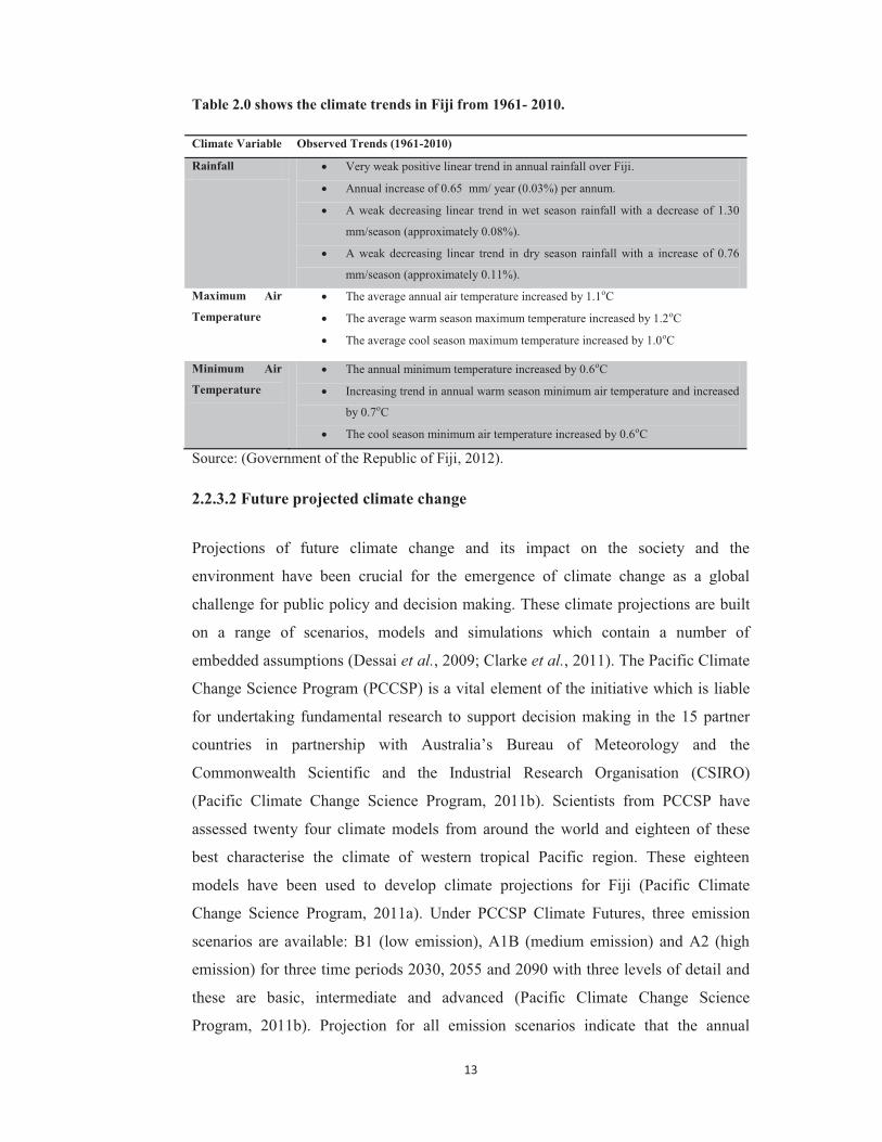
Table 2.0 shows the climate trends in Fiji from 1961- 2010.
Climate Variable Observed Trends (1961-2010)
Rainfall � Very weak positive linear trend in annual rainfall over Fiji.
� Annual increase of 0.65 mm/ year (0.03%) per annum.
� A weak decreasing linear trend in wet season rainfall with a decrease of 1.30
mm/season (approximately 0.08%).
� A weak decreasing linear trend in dry season rainfall with a increase of 0.76
mm/season (approximately 0.11%).
Maximum Air
Temperature
� The average annual air temperature increased by 1.1oC
� The average warm season maximum temperature increased by 1.2oC
� The average cool season maximum temperature increased by 1.0oC
Minimum Air
Temperature
� The annual minimum temperature increased by 0.6oC
� Increasing trend in annual warm season minimum air temperature and increased
by 0.7oC
� The cool season minimum air temperature increased by 0.6oC
Source: (Government of the Republic of Fiji, 2012).
2.2.3.2 Future projected climate change
Projections of future climate change and its impact on the society and the
environment have been crucial for the emergence of climate change as a global
challenge for public policy and decision making. These climate projections are built
on a range of scenarios, models and simulations which contain a number of
embedded assumptions (Dessai et al., 2009; Clarke et al., 2011). The Pacific Climate
Change Science Program (PCCSP) is a vital element of the initiative which is liable
for undertaking fundamental research to support decision making in the 15 partner
countries in partnership with Australia’s Bureau of Meteorology and the
Commonwealth Scientific and the Industrial Research Organisation (CSIRO)
(Pacific Climate Change Science Program, 2011b). Scientists from PCCSP have
assessed twenty four climate models from around the world and eighteen of these
best characterise the climate of western tropical Pacific region. These eighteen
models have been used to develop climate projections for Fiji (Pacific Climate
Change Science Program, 2011a). Under PCCSP Climate Futures, three emission
scenarios are available: B1 (low emission), A1B (medium emission) and A2 (high
emission) for three time periods 2030, 2055 and 2090 with three levels of detail and
these are basic, intermediate and advanced (Pacific Climate Change Science
Program, 2011b). Projection for all emission scenarios indicate that the annual

14
average air temperature and sea surface temperature will increase in the future for
Fiji. It is also projected that increase in mean temperature will also result in an
increase in the number of hot days and warm nights and a decline in cooler weather.
However, there are some uncertainties concerning rainfall and drought projections as
model results are not consistent. Projections from these models indicate that there is
likely to be a decrease in the number of tropical cyclones by the end of 21st century.
However, the intensity of cyclones will increase. There is also likely to be a 2%-11%
increase in the average maximum wind speed of cyclone and an increase of rainfall
intensity of about 20% within the 100km of cyclone centre (Australian Bureau of
Meterology and CSIRO, 2011; Pacific Climate Change Science Program, 2011a).
Recognising the seriousness of climate change concerns, the PICs are implementing
the Pacific Islands Framework on Climate Change 2006-2015. This will aid in
addressing issues of improving the understanding of climate change and providing
training, education and awareness on this matter (Pacific Climate Change Science
Program, 2010). Although the practice of reporting multi-model ensemble climate
projections is well covered, there is still discussion in regards to the most appropriate
levels of evaluating models performance (Irving et al., 2011). Due to the level of
uncertainty attached with climate change projection, it makes it challenging for the
local government to prioritise its commitment to adaptation (SMEC Australia, 2010).
Figure 2.5 shows the atmospheric concentration of atmospheric carbon dioxide for all three
emission scenarios. The projections for amostpheric cardon dioxide concentrations for each
scenario are shown as blue, green and orange. The projections for 2030, 2055 and 2090
(relative to 1990) were calculated using the average value of the 20 year periods 2020-2039,
2046-2065 and 2080-2099 (relative to 1980-1999) to minimise the effect of natural

15
variabilty. The grey bars represent the 20 year periods. Source: (Australian Bureau of
Meterology and CSIRO, 2011; Kumar, 2011).
Table 2.1 shows the projected average annual air temperature change for Fiji under
low emission scenario (B1), medium emission scenario (A1B) and high emission
scenario (B2).
Note: Values represent 90% of the range of models and changes are relative to average
of the period of 1980-1999.
2030 (oC) 2055 (oC) 2090 (oC)
Low Emission Scenario (B1) 0.2-1.0 0.5-1.5 0.7 -2.1
Medium Emission Scenario (A1B) 0.2-1.2 0.9-1.9 1.3-2.9
High Emission Scenario (B2) 0.4-1.0 1.1-1.7 2.0-3.2
Source: (Pacific Climate Change Science Program, 2011a).
2.2.4 Agriculture in Fiji
Agriculture, which was once considered a major stronghold of Fiji’s economy, now
comprises only 16.1 % of the nation’s GDP (CIA World Factbook, 2012b). In 2010
the contribution of the agricultural sector declined by 9.8 % (Bureau of Statistics,
2011). One of the main crops of Fiji is sugar cane which occupies more than 50% of
the arable land and contributes to 9 % of the GDP. The sugar industry engages
almost 13% of the labour force and generates almost 30 % of the export (Rosillo-
Calle and Woods, 2003; Food and Agriculture Organisation, 2009). However, this
industry is facing many challenges such as low investments, uncertain leaseholds and
land ownership rights along with the government’s political instability (CIA World
Factbook, 2012a). Also, the horticultural sector such as ginger, tropical fruits, root
crops and vegetables is now considered the fastest growing agricultural sector.
Traditional tree crops such as cocoa and copra have been deteriorating over the past
decades. Fiji’s import substitution industries consists of rice, dairy, poultry, beef,
pork and tobacco (Food and Agriculture Organisation, 2009).
16
2.2.5 Potato production in Fiji
In recent years, the cultivation of potatoes in lowland tropics, such as Fiji, has gained
popularity. These areas were previously considered unsuitable for potato production
(Iqbal, 1991). More than half of the potatoes in developing countries are cultivated in
warm tropical climates (Midmore and Rhoades, 1988). To maximise potato yield in
the lowland tropics which is characterised by high temperature and high solar
radiation, it is important to maintain high foliage productivity as long as possible
given the fact that growth, development and yield of potatoes is guided by factors
such as high soil and high air temperature, plant density, water stress, availability of
nutrients and the utilisation of solar radiation (Allen, 1978; Ewing, 1981b).
In Fiji, potato was first introduced by European settlers in 1860’s. It was first grown
in Rewa and the crop spread to the Western Division. Between 1937 and 1940, Up
To Date and Early Rose varieties were considered as suitable for local consumption.
Varieties that were suggested in the 1940’s were Brownell and Bismarck (Autar,
2009). Fiji potato acreage in 1981 was around 9 hectares which represented a decline
since 1960 (Iqbal, 1982). Some potential areas for potato production have been
identified and these are Navai, Nadrau Province, Nausori Highlands and Sigatoka
Valley (Autar, 2009). However, one of the major challenges faced by the potato
industry is that of bacterial wilt. To overcome this challenge, the Department of
Agriculture ran a number of unsuccessful experiments with a number of varieties
over the past years. Since the 1970’s, there were introduction of resistant varieties of
potatoes from Mauritius and the International Potato Center (CIP) of Peru. During
1980 and 1991, potatoes worth FJ$2.63 million and FJ$5 million respectively were
imported into Fiji (Autar, 2009). There has always been a potential to grow potatoes
in Fiji, primarily, as a substitute for imports whereby saving foreign exchange.
However, production over the years has varied both in terms of hectare planted and
yield obtained. Variable yield have been obtained in Fiji ranging from 5t/ha to
25t/ha. Production of potatoes is confined to months of May-June to September to
October. In Fiji, Lands Development Authority was a central body that was
responsible for organising large scale planting in mid-1960’s in Nadarivatu, Nausori
Highlands and Sigatoka Valley. Sigatoka Valley has been considered the major
center of production for potatoes with the largest area of production at 134 hectares.
Unfortunately, the Nausori Highlands and Nadarivatu scheme had to come to a stop

17
in 1969 due to high incidence of bacterial wilt. Other challenges to successful growth
of potatoes include: blackleg and root rot, no provision for irrigation during dry
seasons, the attitude of farmers (farmers do not regard potato production as a
business) and potato seeds storage (Iqbal, 1982).
2.3 Origin of potato
Potato, Solanum tuberosum L., is a food crop that is cultivated and consumed
worldwide. It is a basic food source and primary source of income for many of the
communities (Ovchinnikova et al., 2011). Potato made its way around the globe in
the 16th century when the Spanish brought it to Europe from South American Andes.
It later found its way to Asia in the 17th century and to Africa in the 19th century
(Food and Agriculture Organisation of the United Nations, 2008c, d).
Figure 2.6 shows the transfer and spread of potatoes. Source: (The Natural History Museum,
2012).
2.4 Biology of potato
Solanum tuberosum is an herbaceous annual with short vegetative period that grows
up to 100 cm tall and produces a tuber called a potato (Food and Agricultural
Organisation of the United Nations, 2008). It belongs to the family of flowering
plants (Food and Agriculture Organisation of the United Nations, 2008c, d).

18
Table 2.2 shows the taxonomy of potato.
Taxonomic Rank Latin Name
Kingdom Plantae
Phylum Anthophyta
Division Magnoliopsida
Order Solanales
Family Solanaceae
Genus Solanum
Species tuberosa
Common names Potato, tater, spud, tuber
Source: (Bradley, 2009).
In potato, the development of the sprout is dependent on the ageing processes of seed
tuber and is vital for the growth and performance that are taking place in the seed
tuber. This development can be influenced by external factors such as light,
photoperiod, temperature and relative humidity. Many stems can result from a seed
tuber depending on the number of buds. For the duration of the first growing period,
these stems share resources from the same seed tuber and later these stems become
independent units and compete with each other for resources such as light, water and
nutrients. The stems of below-ground part of potatoes are typically round and
massive, whereas in the upper part it is hollow and angular. The potato plant has a
central leaf per node. The early leaves are small but the latter leaves are alternate and
pinnate compound with three or four pairs of large ovate elliptical leaflets with much
smaller leaves found in between. Daylength and temperature also have an influence
on the number of leaves. Long day length and high temperature increase the number
of leaves on secondary stem (Struik, 2007a). At higher temperature, the effect of
photoperiod is stronger. Tuberisation starts before all stolons have been formed. The
tubers begin as stolon swelling and go through different phases of tuber set, tuber
growth and tuber maturation. However, when induction to tuberisation is interrupted,
they can show secondary growth, especially when the plant is exposed to heat or
irregular water supply. The potato has a fibrous root system. The root system is
rather weak and the water and nutrient use efficiency in potato are low. Hence, the

19
crop is very sensitive to drought and poor soil structure. The roots occur not only on
the stems but also on stolons and the tubers (Struik, 2007a).
The potato plant has five growth stages and these are: sprout development, plant
establishment, tuber initiation, tuber bulking and tuber maturation. Depending on the
planting date, physiological age of the seed tubers, cultivar and other environmental
factors, stages I and II last from 30 to 70 days. The period between emergence and
tuber initiation is reduced by short days and temperatures less than 20ºC. The ideal
temperature for the second stage is considered to be between 16ºC-18ºC (van
Heemst, 1986). The third stage, which is tuber initiation, is when tubers start to form
stolon tips. In the fourth stage, the tuber cells start to enlarge due to accumulation of
water, nutrients and carbohydrates. When the conditions are favorable, elongation of
stolons stops and tuber elongation begins (Xu et al., 1998). Depending on the
cultivar, tuber bulking can last up to three months. Tuber maturation is the final stage
where photosynthesis slowly declines, leaves begin to turn yellow, tuber growth
slows and the vines die (Alberta Agriculture Food and Rural Development
Department., 2005).
2.5 Tuber formation and potato nutrient content
Tuber dry matter concentration and tuber size are the two important aspects of
potato. When a tuber is initiated as swelling stolon tip, the dry matter concentration
is about 11%. As the tuber size increases, the dry matter increases along with the
starch. The final dry matter concentration depends on the cultivar, length of growing
seasons, water availability, solar intensity and the average temperature during the
growing season (Haverkort and Verhagen, 2008).
During tuber enlargement, the tuber stores large quantities of carbohydrates (starch
which is 20% of fresh weight) (Fernie and Willmitzer, 2001) and substantial amounts
of proteins and are also low in fat (Food and Agriculture Organisation of the United
Nations, 2008i). It also contains toxins, either natural (example glycoalkaloids) or
food-borne toxins (example acrylamide) (Haase, 2008) and significant amounts of
iron, potassium, zinc, vitamin B and traces of manganese, chromium, selenium and
molybdenum and about half of the daily adult requirement of vitamin C which
enhances iron absorption. An average serving of potatoes with skin has 10 percent of
recommended daily intake of fiber (International Potato Center, 2008a). Potatoes

20
also contribute important amounts of dietary fiber (up to 3.3 %), ascorbic acid (up to
42 mg/100g), potassium (up to 693.8 mg/100g), total caroteniods (up to 2700
mcg/100g) and antioxidant phenols such as chlorogenic acid (up to 1570 mcg/100g)
(Burlingame et al., 2009).
2.6 World potato production
Since the 1960’s, substantial changes have occurred in potato production, types of
potato crops grown and yield in Northern Britain. There is already evidence that
farmers in the northern latitude have already began to adapt to climatic changes such
as warmer temperatures (Plauborg et al., 2010). In the early 1990, majority of the
potatoes were cultivated and consumed in Europe, North America and the former
countries of the Soviet Union. There has been a major increase in potato production
and demand in Asia, Africa and Latin America from 30 million tonnes in 1960 to
more than 165 million tonnes in 2007. One third of the potatoes are now harvested in
China and India (Food and Agricultural Organisation of the United Nations, 2008)
growing 22 % of all potatoes (Jansky et al., 2009). In addition, in harsher climates,
potatoes can produce more nutritious food than any other major crop – up to 85 % of
the crop is edible human food compared to 50 % in cereals. Over the last 10 years,
world potato production has increased at an annual rate of 4.5% and this rate will
increase strongly in the future. This growth has exceeded the production of many
other major food commodities in developing countries (Food and Agricultural
Organisation of the United Nations, 2008).
Potato is regarded as the “frontline in the fight against world hunger and poverty”
(Food and Agricultural Organisation of the United Nations, 2008). The International
Year of Potatoes has contributed to the following United Nations Millennium
Development Goals (MDGs): Goal 1-Eradicate extreme hunger and poverty, Goal 4-
Reduce child mortality, Goal 5-Improve maternal health, Goal 7-Ensure
environmental sustainability and Goal 8-Develop a global partnership for
development (Chiru et al., 2008; Food and Agriculture Organisation of the United
Nations, 2008f, e, b; Thornton et al., 2010). Potato is included in The International
Treaty on Plant Genetic Resources for Food and Agriculture that aims at the
“conservation and sustainable use of crop plant diversity and fair and equitable
21
sharing of benefits derived from their use” (Food and Agriculture Organisation of the
United Nations, 2008a).
2.7 Potato production in Asia and the Pacific region
In many places, such as the highlands of southern China and Vietnam, potato is
emerging as an offseason crop and is being planted as a rotation crop such with rice
and maize. Likewise, in the lowlands of Bangladesh and eastern India, potato is
emerging as a winter cash crop. In Philippines and Indonesia, potato production
satisfies the need for domestic and regional snack food industries. Potato has also
become an important crop in Asia and the Pacific (Changchui, 2008). Three broad
bands of potato production are clearly visible in the Asia-Pacific Region. The first
one runs from west to east across the sup-tropical lowlands of the major river basins
in South Asia and includes Bangladesh, India and Pakistan. The second band runs
from interior of China and ends at Siberian border of Russia. The last band is
characterised by productivity in the Pacific which includes Australia and New
Zealand (Pandey, 2008) and Fiji (Autar, 2009).
In the developing world, potato is crucial to food security. The production of
potatoes has doubled in the last 20 years. Overall the consumption of potatoes has
increased from 9-15 kg/capita and by 2020 the demand for potatoes is anticipated to
double that of 1993. In the Tropics, the farmers can harvest 15-25 tonnes of potatoes
within 90 days of planting. However, there are many challenges that the potato
production faces in the Tropics and Potato Late Blight is one of them affecting 3
million hectares of potato producing land with an estimated damage of $2.75 billion
annually (Food and Agriculture Organisation, 2008).
2.8 Cultivation, harvesting and storage of potato.
Loam or sandy loam soils that are rich in organic matter with good drainage and
aeration and with a pH of 5.2 and 6.4 are appropriate for potato cultivation. In most
cases the soil requires three ploughings with regular hallowing and rolling so that the
soil is well aerated, has good drainage and is soft. Cultivation of potato without
tillage assistances to restore soil fertility, increase potato yields and reduce the need
for fertiliser and fuel (Food and Agriculture Organisation of the United Nations,
2008g). Potato is usually grown from “seed potato”, that are small tubers or pieces of

22
tubers sown to a depth of 5-10 cm. A good seed would usually be disease free, well
sprouted and about 30-40 grams in weight. Small, single eyed seeds are planted 25
cm to 30 cm apart in furrows 60-90 cm apart (Iqbal, 1982). Upon germination, shoots
usually emerge within 21 days. Development of potato canopy takes about 4 weeks
during which weeds must be controlled in order to give the potato crop a
“competitive advantage”. By this time the primary roots have elongated to about 4-6
inches long. During the phase of emergence, nutrients are supplied to the plant
directly from the seed reserves (Lang et al., 1999). Potato cultivation requires very
little labour. Upon maturity, tubers are easily detached from their stolons. The leaves
start to turn yellow indicating maturity. To facilitate harvesting, the potato vines
should be removed two weeks before the potatoes are dug up. Potatoes are usually
harvested using a spading fork. During harvesting it is important to avoid bruising or
other injury which may provide entry points for disease. Proper storage of potatoes is
also vital. If the potatoes are to be stored before consumption, they should be left in
the soil so that the skin of the potato thickens which will prevent storage disease and
shrinkage due to water loss. On the other hand, when left in the ground for too long,
potatoes become susceptible to fungal incrustation called black scurf (Food and
Agricultural Organisation of the United Nations, 2008).
2.9 Physiology of potato
Meteorological factors govern crop productivity by influencing its transpiration,
photosynthesis and respiration in ways to control its growth and development of the
particular crop throughout its physiological cycle at a given site (Pereira et al., 2008).
Among the main environmental factors that govern the growth and development of
plant comprises global solar radiation flux density, air temperature and available soil
water content (Coelho and Dale, 1980), solar radiation, radiation use efficiency,
harvest index (Iqbal, 1991), air temperature, soil temperature, photoperiod, soil
moisture and crop water use (World Meteorological Organisation, 2010).
Potato uses water rather efficiently and has a high harvest index of about 0.75 as
compared to cereals which has a harvest index of 0.5 (Vos and Haverkort, 2007b).
Adequate water is essential for high tuber yield and good tuber quality (World
Meteorological Organisation, 2010). Potatoes usually face water stress due to their
shallow root system (Curwen, 1993). Seventy percent of water uptake occurs at 0.3
23
m and 100 % for upper 0.4 m to 0.6m soil depth (Food and Agriculture Organisation
of the United Nations 2012). For best yields, a 150 day crop requires 500 mm-700
mm of water (Food and Agricultural Organisation of the United Nations, 2008).
Excessive soil moisture can result in seed-piece decay and erratic plant development,
fungal infections such as potato blight, rots and wilts (World Meteorological
Organisation, 2010).
There is a positive relationship between intercepted radiation and the quantity of dry
matter produced (Haverkort, 2007b), the number of tubers (Firman and Daniels,
2011), biomass partitioning (Hoogenboom et al., 1985), leaf area index (LAI) and
the percentage of ground covered by the canopy (Haverkort, 2007a). Tuberisation is
also favourable when plants are exposed to shorter days (Zaag et al., 1986; Garner
and Blake, 1989; Iqbal, 1991; Jackson, 1999; Haverkort, 2007a). LAI is also a
significant property of plant canopy. It is the area of leaves (m2) per area of soil (m2)
(Haverkort, 2007a). Leaf area index of 3-4 is adequate to intercept most of the
incident radiation for maximising the yields of tubers that are grown under temperate
conditions (Harris, 1983).
Temperature also plays a critical role in tuber formation. Potato production is best
suited to temperatures of tropical highlands of 15-18 ºC (Haverkort, 1990). However,
the optimal temperature for potato production is 22 ºC (Burton, 1981). Warm
temperatures favour vegetative growth (Ewing and Struik, 1992) while cool
temperature favour tuber growth (Ewing, 1981c; Khedher and Ewing, 1985). Cool
night temperatures are required by potatoes for tuberisation. Changes in temperature
and rainfall pattern affects root crops (Gawander, 2007). Positive effects of elevated
carbon dioxide have also been observed on the yield (Wheeler et al., 1991;
Schapendonk et al., 1995; Miglietta et al., 1998; Rosenzweig and Hillel, 1998; Te
mmerman et al., 2000; Lawson et al., 2001b; Te mmerman et al., 2002; Persson et
al., 2003; Te mmerman et al., 2007; Bindi, 2008).
Nitrogen uptake efficiency of potatoes under current best practice management is
approximately 65 %, an efficiency rate which is comparable to that of corn and
wheat (Lang et al., 1999). The first in-season nitrogen application should occur after
tuber initiation as during this stage 30-40 % of nitrogen has been taken up. It is also

24
crucial to maintain nitrogen levels during tuber bulking which is considered as an
important stage in potato development (Lang et al., 1999). The requirement of
nitrogen fertiliser ranges from 2.5 to 5.9 kg ha-1 per tonne of tuber yield (Hagman et
al., 2009). To cater for the nitrogen needs of this crop, nitrogen fertilisers can be
supplied in many ways: ammonia, nitrate, urea (Bucher and Kossmann, 2007).
Nitrogen uptake is also cultivar specific (Love et al., 2005; Fontes et al., 2010).
There are also many pests of potatoes that can reduce both tuber yield and quality
(Food and Agriculture Organisation of the United Nations, 2008h), such as Colorado
potato beetle (Leptinotarsa decemlineata), potato tuber moth (Phthorimaea
operculella), leaf miner fly (Liriomyza huidobrensis), serious soil pests of potato in
the temperate regions, such as, Globodera pallid and G. rostochiensis, potato Late
Blight (Phytophthora infestans) (Świeżyński and Zimnoch-Guzowska, 2001;
International Potato Center, 2008a; Cooke et al., 2011), bacterial wilt and Potato
Blackleg (International Potato Center, 2008b) and aphids as virus vectors (Food and
Agriculture Organisation of the United Nations, 2008d). Due to climate change, the
break out period of pest and disease will become earlier than expected (Hannukkala
et al., 2007) with expansion into areas that were previously safe from this disease.
Little effort has been made to document the non-targeted impacts of pesticides on
potatoes (Thornton et al., 2010) .
2.10 Climate model system in prediction of agriculture and crop growth
The most managed ecosystem in the world is agriculture (Stoorvogel et al., 2004).
Agriculture deals with diverse range of issues, such as, sustaining agricultural
livelihoods, protecting water quality and other resources and climate change
mitigation strategies. All these demand the need to create information to make
informed decision on how agricultural systems respond to changes in external
stimuli, such as, changes in technology, policies and climate change (Stoorvogel et
al., 2004). A lot of emphasis is being employed in estimating crop productivity as a
function of climatic elements by different weather models (Pereira et al., 2008). Crop
modeling began since 1960’s (Bouman et al., 1996) and has extensively developed
over the last 30 years (Kumar et al., 2000). Crop simulation models are a
representation of a simplified crop production system made up of non-linear
mathematical equations to provide a systematic analysis of the crop production

25
system (Easterling et al., 1996). Crop growth models are complex as they require a
series of complex interaction between soil, plant, weather and growth reducing
factors such as pest, disease and weeds (Singh, 1999). These need to be accurately
represented in order to produce a reliable picture. The crop models used today are of
a multi-disciplinary approach with environmental impact models and economic
models linked together (Bosello and Zhang, 2005). A total of 104 countries were
reported having utilised modeling done at individual sites within these countries
(Rivington and Koo, 2010). Crop models aim to explain crop development and
behaviour, yield and quality as a function of environmental variables, genetic
variables and disease (MacKerron, 2007). In most crop models, growth and
development are driven by solar radiation. However, in some models, temperature
plays a more dominant role than solar radiation (MacKerron, 2007). Crop modeling
requires input data of weather, soil, crop management data and pest data
(Chakrabarti, 2005). Some of the widely accepted plant physiology models include
CERES-Maize, CERES-Wheat, CERES- Rice (Singh et al., 1993), SOYGRO (Jones
et al., 1988), SIM-POTATO (Bosello and Zhang, 2005), CropSyst (Stockle et al.,
2003), EPIC model (Bulatewicz et al., 2009; Pumijumnong and Arunrat, 2012),
APSIM (Cheeroo-Nayamuth, 1999), Tradeoff Analysis Model (Stoorvogel et al.,
2004) and CANEGRO (Cheeroo-Nayamuth, 1999). Models can also be linked to
other models to gather more information on crop growth and development (Roth et
al., 1991).
Potato crop modeling developed and started in the late 1970’s. The earliest potato
models attempted to represent the typical characteristics of potatoes such as growth
pattern, effect of temperature, day length and cultivar (Ng N and Loomis, 1984).
Later, potato models looked at approximation of potato yield based on solar radiation
and the length of growing season (MacKerron, 2007). Growth rate in many potato
models is calculated on the basis of light interception (Haverkort and MacKerron,
1995). Numerous efforts have been made to simulate potato growth and development
(Te mmerman et al., 2007), leaf area index (Van Delden A et al., 2001; Gonzalez-
Sanpedro et al., 2009), tuber fresh weight (Medany, 2006), comparison of present
yield and predicted yield using the climate change data (Abdrabbo et al., 2010), to
study the interaction of water and nitrogen supply and weather variability (Bowen,
2003), the influence of water supply and potential evaporation on growth and

26
development of potatoes and the effect of length and temperature on potato growth
and development (MacKerron, 2007) and pathogenic fungus infection on potatoes
(Iglesias et al., 2007). A common figure of models is that they are usually location
and cultivar specific. Hence, by limiting the geographical locations, the
environmental inputs required to run the model also becomes limited (Griffin et al.,
1993). Although tuber initiation is sensitive to photoperiod, a number of models
ignore the effect of photoperiod on tuber initiation. Other models, such as POMOD
(Kadaja and Tooming, 2004), SIMPOTATO (Rosenzweig et al., 1996), LINTUL
(Haverkort et al., 2004), AQUACROP (Patel et al., 2008), TUBERPRO and
LINTUL-POTATO (Kooman and Haverkort, 1995) also exist that can be used to
determine potential potato yield.
One of the most widely used crop model is Decision Support System for
Agrotechnology Transfer (DSSAT) which was developed by International
Benchmark Sites Network for Agrotechnology Transfer (IBSNAT). The DSSAT
model incorporates 27 different crop models, such as, cereal grain, legumes and root
crops (Hoogenboom, 2003). DSSAT has been registered in 100 countries (Rivington
and Koo, 2010). The IBSNAT crop models were used to estimate how climate
change will affect crops at 112 sites in 18 countries, representing key production
areas and vulnerable regions at low, mid and high latitudes. DSSAT was successful
in predicting the relative nitrogen rates and potato nitrogen uptake for six different
fertility scenarios centered on different organic and inorganic nitrogen source
combinations (Snapp and Fortuna, 2003). The DSSAT SUBSTOR Potato model has
a great potential to simulate potato growth and evaluating potential changes in
management in many regions (Griffin et al., 1993). It also has the capability to
simulate on a daily basis the growth and development potato crop using data such as
on climate, soil, management and cultivar (Jones et al., 2003; Knox et al., 2010). The
DSSAT SUBSTOR Potato model is branched into four main sub-models which are:
phonological development, biomass formation and portioning, soil water and
nitrogen balance which work simultaneously to provide a realistic description of the
plant-soil-atmosphere system. The genetic-coefficient is used by the model to control
development phases, such as, tuber initiation, leaf area development and tuber
growth rate. The DSSAT SUBSTOR model has been extensively used for global
crop studies and recently for climate change impacts. The reason for its widespread

27
use is due to its ability to simulate canopy response to temperature and radiation
change to incorporate the direct effects of atmospheric carbon dioxide on potato
production (Knox et al., 2010). The DSSAT SUBSTOR Potato model has also been
validated in many areas and used to simulate physiological processes and yield of
potatoes under current climatic and future conditions (Bowen et al., 1998;
International Potato Center, 1999; Fleisher et al., 2003; Štastna and Dufkova, 2008;
Abdrabbo et al., 2010; Knox et al., 2010). To simulate the response of different plant
organs and processes over a wide temperature range, the DSSAT SUBSTOR Potato
model uses zero to one relative temperature functions based on mean daily air or soil
temperature. The timing of tuber initiation in the DSSAT SUBSTOR Potato model is
a function of cultivar response to temperature and photoperiod, plant nitrogen status
and soil water status. The DSSAT SUBSTOR Potato model does not simulate the
development of individual leaves but rather the development of the entire canopy
(Griffin et al., 1993). The model also shows poor performance for LAI (as compared
to tuber initiation) due to lack of disease or insect defoliation subroutines in the
model (Griffin et al., 1993; Parry, 2007). The simulation of tuber yield by
SUBSTOR model is also accurate (Griffin et al., 1993).
Crop simulation models have become accurate enough and have become widely
accepted (Easterling et al., 1996). A number of opportunities are now available
through the use of crop models, such as, determining the potential and attainable
yield for various crops, optimising crop management, evaluating the impact of
climate change, forecasting crop yields, estimation of crop growth and yield under
climate variability and increasing the efficiency of multi-environment testing (Singh,
1999), promotes interdisciplinary collaboration (Chakrabarti, 2005), for decision
support system, education and training, research for crop genetic improvement,
policy development (Rivington and Koo, 2010) and statistical links between weather
and yield can also be useful for economic modeling (Roberts et al., 2013).
While crop models have been successful tools in application, they all have their
weakness and fail under certain circumstances (Graeff et al., 1999). The complexity
of real world cannot fully expressed in any model (Raisanen, 2007). Agricultural
interactions are complex that are not fully understood. Hence, the models are a crude
representation of reality. Model quality is also depended on the quality of scientific

28
data used in model development, calibration and validation. When models are
applied in new situations, model calibration and validation are needed to verify the
model because all processes are not understood and the model contains parameter
adjustments to new situations (Cheeroo-Nayamuth, 1999). Other drawbacks
encountered in the use of crop models include the availability of reliable data as
input (Singh, 1999), lack of skilled manpower, lack of knowledge on computer and
computer language, limited awareness and acceptance towards modeling, existing
complexity of biological systems are hard to replicate in models giving rise to
uncertainties and errors, models developed for one specific region cannot be used in
another region until the model is calibrated (Chakrabarti, 2005) and difficulty in
simulating root mass (MacKerron, 2007).
2.11 Implication of study
This research aims to investigate the impact of climate change and climate variability
on Potato production in Fiji. The DSSAT SUBSTOR Potato model was calibrated for
the first time in Fiji using Desiree variety. Potato growth, development and yield
were assessed under current weather conditions and climate variability. Potato
production was also simulated under future climatic scenario using PCCSP medium
(A1B) and high (A2) emission scenarios. Optimisation treatment for crop
management strategies were also carried out for current and future climatic
conditions to sustain potato yields. Finally, through Sensitivity Analysis the best
cultivar was identified for both current and future climatic conditions. It is hoped that
this research will help us to understand the impacts of climate change and climate
variability on potato production in Fiji. It will advise policy makers and farmers on
suitable adaptation measures to improve potato production and contribute to
improvement in livelihood and food security. Furthermore, since this is the first time
that DSSAT SUBSTOR Potato model was calibrated in the Tropical region, it will
deliver an insight on its performance in simulating potato growth in warmer climates.
This knowledge will also help crop model developers to re-adjust crop models and
their performance to real variables in the Tropics. This research will also contribute
to the awareness of impacts of climate change on root crops in the Pacific Island
Countries which will be important for UNFCCC documents such as IPCC reports.

29
Chapter 3 Calibration of DSSAT SUBSTOR Potato Model
3.0 DSSAT overview DSSAT is a personal computer-based program comprising of crop models and data
base management programs for climate, soil and crop management practices
(Rosenzweig and Parry, 1994). Based on the soil-plant-atmosphere dynamics, the
DSSAT crop models can simulate growth, development and yield (Jones et al.,
2003). For data input, daily weather data, soil surface and soil profile information,
and detail crop management data is required by the model. The weather conditions
that are needed to run the model include daily values for minimum and maximum air
temperature, total precipitation, and total solar radiation. Other variables that are
required include latitude to calculate day length and carbon dioxide concentration of
the atmosphere (Hoogenboom et al., 1985).
Before a model is simulated for a particular region, it should be calibrated and
validated. Calibration and validation are two different processes. Calibrated models
have become a significant tool for economic research and policy analysis (Cooley,
1997). Model calibration is defined as adjusting an already existing model to a
reference system. It is necessary to calibrate the model in order to get reliable results
since the model is based on abstractions, idealisation and many disputable
assumptions (Hofmann, 2005). In calibration, model parameters and coding are
changed in order to obtain the best fit for simulation versus observed data (Boote,
1999).
One important task in working with models is testing their performance in wide
range of circumstances so that one is able to identify their scope of validity and
limitations. This is because simulation models are site and crop specific in nature and
cannot be utilised in other areas unless validated under local conditions (Ahmed and
Fayyaz-ul-Hassan, 2011). However, the process of evaluation can be time consuming
and challenging because it requires the collection of large data sets such as weather
data, soil data, crop and field management information over long time periods
(St’astna et al., 2002). A research conducted in Malawi from 1990-1993 aimed to
validate the CERES-Maize model. The results showed that the model worked

30
reasonably well with grain yield (Singh et al., 2002). Various components of
CERES-Rice model have also been validated (Singh and Ritchie, 1993). To validate
the DSSAT SUBSTOR Potato model, that is, to compare model simulated yield to
observed data, formatted yield data is required (Thorpa et al., 2008). The comparison
of simulated and observed data requires retrieval of observed data and converting it
to DSSAT SUBSTOR Potato model format, and comparing simulated outcomes with
observed values (Abdrabbo et al., 2010).
3.1 Methodology
3.1.1 Experimental site
The potato experimental replicate plot was located in Banisogosogo, Rakiraki
(longitude 17˚ 22' 00" South and latitude 178˚ 9' 00" East) (National Geospatial-
Intelligence Agency, 2012b). Rakiraki, which is on the main island of Viti Levu, is a
district in Ra province which is situated halfway between Suva and Nadi along the
Kings Road on the Northern Coast of Viti Levu, Fiji’s largest Island (Urbita, 2012).
Figure 3.0 shows the location of experimental site (Banisogosogo). The experimental plot is
located in the Western Division of Viti Levu. Source: (GoogleEarth, 2012).
31
3.1.2 Climate trends of field site
Banisogosogo (Rakiraki) is located on the Western side of Viti Levu. The Western
Division is the dry zone and is subjected to large seasonal and inter-annual climatic
variation. The annual average surface air temperature increase for Penang (Rakiraki)
is 0.17 oC, with an increase of 0.05 oC per decade. The average yearly rainfall in
Rakiraki is about 2000 mm. During the winter weather in this area, it is clear or
partly cloudy with plenty of sunshine and a well-developed west to north-westerly
winds by day and south easterlies are prominent wind at night and in all months
except for August to March. From August to March the wind is mostly from north
westerly quarter. The nights are relatively cool in this season. However, during
summer there is thunderstorm activity which is responsible for brief but intense
rainfall (Gawander et al., 2012). According to the hybrid climate data obtained from
Fiji Meteorological Services (FMS) and National Aeronautics and Space
Administration (NASA), the average maximum temperature is 29.09 oC while the
average minimum temperature is 22.4 oC.
3.1.3 Reason for site selection
Banisogosogo was selected as the site for experimental replicate plot to calibrate the
DSSAT SUSTOR Potato model because the Agriculture Department of Fiji has
started to distribute potato seeds to farmers at Rakiraki for potato cultivation. This
site was also selected due to logistic reasons, that is, the land owner of the
experimental replicate plot was a family friend which ensured that the experimental
replicate plot was not disturbed.
3.1.4 Data collection, treatments and importations
3.1.4.1 Weather data
The 30 year climatic data for Penang, Rakiraki (which represented weather data of
the experimental replicate plot), such as, daily maximum temperature (Tmax) (oC)
and minimum temperature (Tmin) (oC), and precipitation ( mm) were collected from
the Sugar Research Institute of Fiji (SRIF) and FMS. Solar radiation of the
experimental site was downloaded from the NASA website. When the weather data
had missing values for rainfall and/or temperature they were replaced with NASA
data creating a “hybrid” weather data. The DSSAT format weather data was created

32
in Excel worksheet. This excel worksheet was then imported into WeatherMan tool
in DSSAT. WeatherMan has the ability to produce complete sets of weather data
historically or synthetically created records (Singh et al., 2002).
3.1.4.2 Soil data
There were three replicate experimental plots. Soil samples were collected from each
replicate plot. Using randomised complete block design, nine random sampling pits
were dug, three in each replicate plot. One sample per layer was taken from each
sampling pit of each replicate plot. The soil samples were taken from 0-40 cm, 40-
100 cm and +100 cm. The soil samples were placed in a bucket and samples were
mixed. Stones, plant materials were removed while mixing. From the bucket, 1 kg of
soil was removed and it was placed in sampling bags and sealed tightly. This was
then given to Koronivia Research Station for chemical analysis (pH, organic carbon
and Cation Exchange Capacity). This was done before the planting began. The soil
data was entered into SBuild tool of DSSAT SUBSTOR Potato model.
The soil characteristics that are needed to run the model include albedo of bare soil,
soil surface runoff (expressed as runoff curve number), first stage soil evaporation,
water permeability and drainage from profile. For each layer the following variables
are required: layer thickness, saturated soil water content, drained upper limit of
extractable plant water (field capacity), permanent wilting point, initial soil water
content at the start of soil water balance simulation and relative root weighing factor
(Hoogenboom et al., 1985).
DSSAT’s SBuild tool estimates the above input based texture and organic matter
when actual measurements are not available. Default Medium Silty Clay from
DSSAT soil database was used to calculate model inputs. A conversion factor based
on measured (Banisogosogo soil) and estimated (default soil) bulk density was used
to recalculate the bulk density, soil lower limit, soil upper drainage limit and the soil
saturation for the Banisogosogo soil (replicate plot 1, replicate plot 2 and replicate
plot 3). The conversion factor was calculated by dividing the Default Medium Silty
Clay soil by the bulk density of replicate plot 1, Banisogosogo soil. This gave us the
conversion factor. The replicate plot 1 bulk density was then multiplied by the
conversion factor to obtain the recalculated bulk density. The same procedure was

33
repeated for Lower Limit, Drained Upper Limit and Saturation. This procedure was
used to ensure the values for soil lower limit, drained upper limit, and the saturated
water content were realistic and not biased by the high clay content of Banisogosogo
soil. The calculated values for the lower limit < than drained upper limit < saturated
water content < pore volume fraction.
3.1.4.3 Experimental replicate plot
The experimental replicate plot was located in Banisogosogo, Rakiraki, Fiji. Potato
seeds were planted in 11 rows and 17 columns with a row spacing of 75 cm and 30
cm within the rows (Agriculture Department of Fiji, 2009). The experimental
replicate plot had a length of 7.5 m and a width of 4.8 m (total area was 36 m2 or
0.0036 hectares). Rows 1 and 11 acted as border plants. Rows 2-4 were replicate plot
1, rows 5-7 were replicate plot 2, rows 8-10 were replicate plot 3. Ten columns
allowed harvesting of 2 plants per row, that is, 6 plants for each replicate plot (T1,
T2, T3) with a total of 18 plants for each sampling time and T4 allowed harvesting of
4 plants per row, that is, 12 plants per replicate plot with a total harvest of 36 plants.
The potatoes were planted on 2nd of July 2012 at a depth of 1.5 cm.
Figure 3.1 shows collection of sample soil (left) and marking of replicate plot (right).
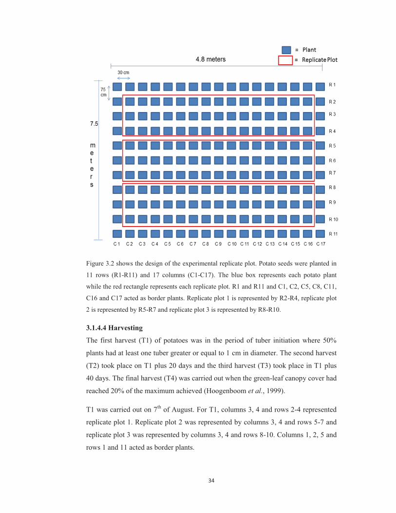
34
Figure 3.2 shows the design of the experimental replicate plot. Potato seeds were planted in
11 rows (R1-R11) and 17 columns (C1-C17). The blue box represents each potato plant
while the red rectangle represents each replicate plot. R1 and R11 and C1, C2, C5, C8, C11,
C16 and C17 acted as border plants. Replicate plot 1 is represented by R2-R4, replicate plot
2 is represented by R5-R7 and replicate plot 3 is represented by R8-R10.
3.1.4.4 Harvesting
The first harvest (T1) of potatoes was in the period of tuber initiation where 50%
plants had at least one tuber greater or equal to 1 cm in diameter. The second harvest
(T2) took place on T1 plus 20 days and the third harvest (T3) took place in T1 plus
40 days. The final harvest (T4) was carried out when the green-leaf canopy cover had
reached 20% of the maximum achieved (Hoogenboom et al., 1999).
T1 was carried out on 7th of August. For T1, columns 3, 4 and rows 2-4 represented
replicate plot 1. Replicate plot 2 was represented by columns 3, 4 and rows 5-7 and
replicate plot 3 was represented by columns 3, 4 and rows 8-10. Columns 1, 2, 5 and
rows 1 and 11 acted as border plants.
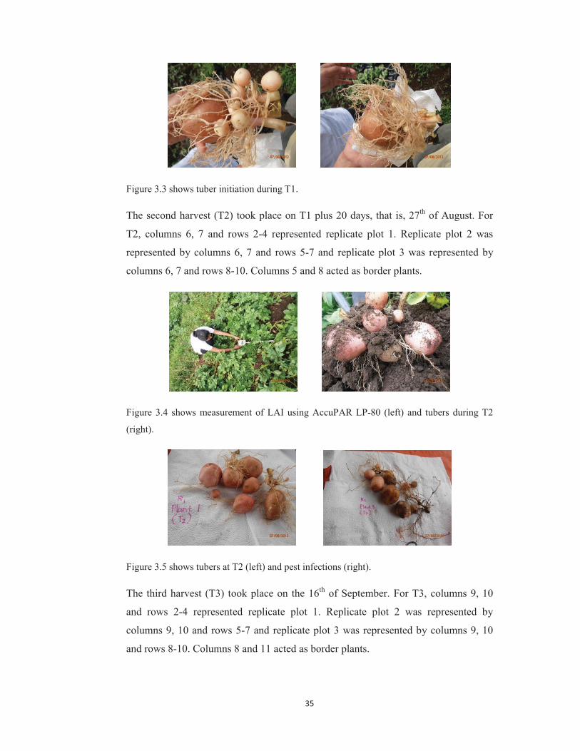
35
Figure 3.3 shows tuber initiation during T1.
The second harvest (T2) took place on T1 plus 20 days, that is, 27th of August. For
T2, columns 6, 7 and rows 2-4 represented replicate plot 1. Replicate plot 2 was
represented by columns 6, 7 and rows 5-7 and replicate plot 3 was represented by
columns 6, 7 and rows 8-10. Columns 5 and 8 acted as border plants.
Figure 3.4 shows measurement of LAI using AccuPAR LP-80 (left) and tubers during T2
(right).
Figure 3.5 shows tubers at T2 (left) and pest infections (right).
The third harvest (T3) took place on the 16th of September. For T3, columns 9, 10
and rows 2-4 represented replicate plot 1. Replicate plot 2 was represented by
columns 9, 10 and rows 5-7 and replicate plot 3 was represented by columns 9, 10
and rows 8-10. Columns 8 and 11 acted as border plants.

36
Figure 3.6 shows nematode infection (left), beetle infection (Papuana spp.) (center) and pest
Quantula striata.(right).
T4 was carried out on 20th of September. Columns 12-15 and rows 2-4 represented
replicate plot 1. Replicate plot 2 was represented by columns 12-15 and rows 5-7 and
replicate plot 3 was represented by columns 12-15 and rows 8-10. Columns 11, 16,
17 acted as border plants. For each harvest (T1, T2, T3), 2 plants per row were
harvested from each replicate plot, giving a harvest of 6 plants per replicate plot with
a total of 18 plants harvested for all 3 replicate plots. T4 allowed harvesting of 4
plants per row, that is, 12 plants per replicate plot with a total harvest of 36 plants.
Figure 3.7 shows tubers during final harvest and pest infection (right).
3.1.4.5 Fresh aboveground biomass collection
For the aboveground biomass (stem and leaves), the stems were cut as closely to the
ground as possible with a garden pruner. The above ground mass was cleaned by
washing it in a bucket of water until all the dirt was removed. This was then blotted
dry with tissue paper. The weight of the whole above ground biomass was taken on a
digital scale and recorded. The leaves and stems were then separated and weighed
individually. The number of stems and compound leaves for each plant was also
recorded.

37
3.1.4.6 Fresh belowground biomass collection
To take the below ground mass (roots and tubers), the belowground mass was first
cleaned by washing it in a bucket of water until all the dirt was removed and blotted
dry with tissue paper. The whole belowground mass was recorded. The roots, tubers
and mother tuber were then separated and weighed individually. The number of
tubers per plant was also recorded.
3.1.4.7 Dry biomass
The weight of empty brown paper bag was taken. Individual plant components were
then put in brown paper bag and labeled with a pencil. This was then oven dried in
Ontherm Thermotec 2000 at 70oC regularly until the weight was stabilised.
3.1.4.8 Leaf Area Index (LAI)
A portable leaf area meter (LAW-A) was used to calculate the LAI. The LAI for T1
was calculated by using the formula: LAI = (LAM. N)/A, where, N represents the
number of leaves in the plant and A is the area occupied by one plant (Blanco and
Folegatti, 2003).
From T2, the leaf area index was taken using AccuPAR LP-80. The AccuPAR LP -
80 was first configured by entering information such as longitude, latitude, date/time,
daylight saving time, leaf distribution and the external sensor constant. The external
sensor was then attached to AccuPAR LP-80. When the PAR readings were above
600 µmol/m2s and the probe and the external sensor were leveled and the AccuPAR
was calibrated. Only 3 segments out of 8 segments in the probe were activated and
an external sensor was allowed to make simultaneous readings both above and below
canopy. The probe was extended from one mid row to the next mid row. This
allowed to obtain a good representative sample of the area below and between rows
(Decagon Devices, 2006).
3.1.5 Rainfed and nitrogen response experiment
The Rainfed and Nitrogen Response Experiment were also created to determine the
nitrate and ammonia levels in the soil in order to calibrate the model.
38
3.1.6 DSSAT SUBSTOR Potato model calibration
3.1.6.1. AFile (Average File)
AFile was used to generate the measured data for simulation comparison. The
average of T4 harvest was used to create AFile. Data was entered into Excel
Worksheet and imported into DSSAT SUBSTOR Potato model under Experimental
data. The following are the information that was entered into AFile excel:
� TRNO- treatment number (each replicate plot was considered as a
treatment)
� UWAH- tuber dry weight (kg/ha)
� UYAH- tuber fresh weight (t/ha)
� LAIX- leaf area index, maximum
� BWAH- by product removed during harvest (kg (dm)/ha)
� TDAT- tuber initiation date (Julian Date Format)
� HDAT-harvest date (Julian Date Format)
3.1.6.2. TFile (Time Series File)
TFile, or Time Series Data, was created by taking into consideration the average of
all the T series, that is, T1, T2, T3 and T4. Data was entered into Excel Worksheet.
This data was imported into DSSAT SUBSTOR Potato model under Experimental
data. The following are the information that was entered into TFile excel:
� TRNO- treatment number (for each replicate plot T1, T2, T3 and T4 data was
considered)
� Date- for each Time Series in Julian Date Format
� LAID- leaf area index
� UWAD- tuber dry weight (kg/ha)
� UYAD- tuber fresh weight (t/ha)
� LWAD- leaf dry weight(kg/ha)
� SWAD- stem dry weight(kg/ha)

39
3.1.7 Genetic co-efficient adjustments
Since the DSSAT SUBSTOR Potato model had never been tested in the Tropical
regions before, the genetic co-efficient was adjusted directly in the Genetic File by
comparing the simulation results for phenology (tuber initiation, maturity) and
growth (tuber numbers, yield) with observed results.
A similar procedure for the collection of field-data has been described in previous
studies (Manrique and Bartholomew, 1991; Manrique et al., 1991; Medany, 2006;
Štastna and Dufkova, 2008; Abdrabbo et al., 2010; Knox et al., 2010).
Table 3.0 shows the planting information. This information was required to run
DSSAT SUBSTOR Potato model for calibration.
Variable Information
Cultivar Desiree
Starting Date June 1st 2012
Planting Date July 2nd 2012
Harvest Date September 20th 2012
Planting Method Dry seed
Planting Distribution Rows
Row Spacing 75 cm
Plant Population (m2) 4.4
Planting Depth 1.5 cm
Irrigation 14 mm in 4 application
N-fertiliser (N.P.K fertiliser) 80kg/ha in 2 application (5 grams per plant, banded
beneath the surface at 5 cm depth)

40
Table 3.1 shows the DSSAT SUBSTOR Potato model input and data requirement.
Input
Daily weather Daily Tmax and Tmin (oC), precipitation ( mm) and solar radiation (MJ m-2d-1)
Site Latitude, albedo, surface runoff
Soil (by layer) pH, organic carbon content, depth of each layer ( cm), drained upper limit water
content, saturated water content, bulk density
Cultivar Variety name and genetic co-efficient
Management Planting date, population density, planting depth, row spacing
Development Emergence, floral initiation, maturity date
Water balance Soil water content
Nitrogen Soil nitrogen content
Source: (Singh et al., 1990).
3.1.8 Analysis and outputs
The DSSAT SUBSTOR Potato Model was calibrated using the local experimental
field data, local soil and weather data of the growing season (minimum data set). The
genetic co-efficient was recalibrated directly in the Genetic File (as mentioned in
section 3.1.7) in order to obtain new values for genetic co-efficient parameters. These
inputs were then used in model runs and adjusted in order to obtain a best fit between
simulated and observed data. All summary outputs, graphical outputs and initial
analysis were done in DSSAT 4.5 Output and SBUILD Program. Other statistical
analysis was conducted in 2007 Microsoft Excel Spreadsheet. All these outputs are
provided in the Results section.
3.2 Results
This chapter describes the steps taken to calibrate the DSSAT SUBSTOR Potato
model. The field experiment was carried out at Banisogosogo, Fiji during the potato
growing season (July-September) of 2012 using Desiree variety. Three minimum
data sets were needed to evaluate the model and these included soil data, weather
data and crop management data.
The simulation results before calibration indicated that the simulated values were not
in agreement with the observed values (Table 3.8 and Figure 3.10). The calibration
process included the recalculation of soil water content (Table 3.4) and recalibration

41
of the genetic-co-efficient of Desiree variety (Table 3.9). However, after calibration,
the results showed that there was a good agreement between simulation and observed
values (Table 3.10, Figures 3.11 and 3.12).
3.2.1 Soil information and water content recalculation
The soil samples were collected on 2nd July 2012. For soil data, soil chemical and
physical properties were analysed. The chemical test was conducted for pH,
electrical conductivity (EC), percentage of total carbon and nitrogen, cation
exchange capacity (CEC), exchangeable potassium (K) and moisture levels for each
layer of the three replicate plots. Replicate plot 2 shows the highest percentage of
carbon and nitrogen.
Table 3.2 shows the chemical properties of Banisogosogo soil for each replicate plot.
Replicate Plot pH EC (mS/ cm)
Total C (%)
Total N (%)
CEC ( cmol(+)/kg)
Exchangeable K (me/100g)
Moisture
Replicate plot 1 (0-40 cm)
6.5 0.1 2.32 0.19 40.85 0.75 8.2
Replicate plot 1 (40-100)
6.9 0.07 1.92 0.16 43.43 0.24 7.6
Replicate plot 1 (100-110 cm)
7.0 0.06 1.74 0.14 38.96 0.2 8.3
Replicate plot 2 (0-40 cm)
6.7 0.1 3.51 0.29 41.27 0.84 9.0
Replicate plot 2 (40-100)
7.0 0.06 2.27 0.19 37.43 0.24 6.1
Replicate plot 2 (100-110 cm)
7.1 0.05 1.74 0.14 43.71 0.21 8.1
Replicate plot 3 (0-40 cm)
6.8 0.09 2.14 0.18 36.49 0.56 8.8
Replicate plot 3 (40-100)
7.0 0.06 2.32 0.19 43.49 0.21 8.2
Replicate plot 3 100-110 cm)
7.2 0.06 1.74 0.14 43.94 0.2 8.1
The results for physical properties (Table 3.3) indicated that the overall texture of the
soil was clay. There was very low percentage of silt in the soil.

42
Table 3.3 shows the physical properties of Banisogosogo soil for each replicate plot.
Replicate Plot Clay (%)
( <0.002 mm)
Silt (%)
(0.002-0.06
mm)
Sand (%)
(0.06-2 mm)
Texture
Replicate plot 1 (0-40 cm) 57 23 20 Clay
Replicate plot 1 (40-100) 59 22 19 Clay
Replicate plot 1 (100-110
cm)
44 31 25 Clay
Replicate plot 2 (0-40 cm) 48 25 27 Clay
Replicate plot 2 (40-7.1100) 57 22 21 Clay
Replicate plot 2 (100-110
cm)
56 11 33 Clay
Replicate plot 3 (0-40 cm) 59 25 16 Clay
Replicate plot 3 (40-100) 51 26 23 Clay
Replicate plot 3 (100-110
cm)
63 9 28 Clay
Due to high percentage of clay in the soil, the bulk density, lower limit, drained
upper limit and saturation were recalculated using a conversion factor from Default
Medium Silty Clay to adjust the water level in the soil for model calibration process.
Table 3.4 shows the recalculated water content of bulk density, lower limit of
extractable soil water, drained upper limit and saturation for Banisogosogo soil.
Bulk Density Drained Lower Limit Drained Upper Limit Saturation
Soil
depth
( cm)
Rep 1 Rep 2 Rep 3 Rep 1 Rep 2 Rep 3 Rep 1 Rep 2 Rep 3 Rep 1 Rep 2 Rep 3
0-40 1.24 1.25 1.25 0.26 0.256 0.267 0.40 0.407 0.408 0.51 0.521 0.519
40-
100
1.25 1.23 1.23 0.29 0.294 0.271 0.43 0.435 0.417 0.52 0.516 0.497
100-
110
1.23 1.27 1.22 0.21 0.248 0.273 0.34 0.357 0.357 0.51 0.501 0.49
3.2.2 Weather information
The weather information of the growing season indicated that the highest solar
radiation, Tmax, Tmin and rainfall were received beginning of the year (January,
February and March). On the other hand, during the planting season, which was from
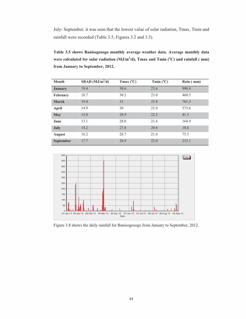
43
July- September, it was seen that the lowest value of solar radiation, Tmax, Tmin and
rainfall were recorded (Table 3.5, Figures 3.2 and 3.3).
Table 3.5 shows Banisogosogo monthly average weather data. Average monthly data
were calculated for solar radiation (MJ/m2/d), Tmax and Tmin (oC) and rainfall ( mm)
from January to September, 2012.
Month SRAD (MJ/m2/d) Tmax (oC) Tmin (oC) Rain ( mm)
January 19.4 30.6 23.6 990.4
February 18.7 30.2 23.0 460.5
March 19.4 31 23.8 761.3
April 14.9 30 23.0 575.6
May 15.0 28.9 22.3 41.3
June 13.1 28.0 21.6 164.9
July 14.2 27.8 20.6 18.6
August 16.2 28.7 21.6 75.3
September 17.7 28.9 22.0 215.1
Rain
Date01-Jan-12 29-Jan-12 28-Feb-12 30-Mar-12 30-Apr-12 01-Jun-12 01-Jul-12 29-Jul-12 28-Aug-12 29-Sep-12
500
450
400
350
300
250
200
150
100
50
0
Figure 3.8 shows the daily rainfall for Banisogosogo from January to September, 2012.

44
TMAXTMIN
Date01-Jan-12 28-Jan-12 28-Feb-12 30-Mar-12 30-Apr-12 31-May-12 01-Jul-12 29-Jul-12 28-Aug-12 29-Sep-12
3432302826242220181614121086420
Figure 3.9 shows the daily maximum and minimum temperature for Banisogosogo from
January to September, 2012.
3.2.3 Experimental file
The crop data, that is, LAI and fresh and dry aboveground and belowground biomass
were entered into the DSSAT SUBSTOR Potato model as an experimental file. The
experimental file included the AFile and the TFile. The AFile was the average final
harvest value (T4) from each treatment (TRNO), for tuber dry weight (UWAH),
tuber fresh weight (UYAH), leaf are index, (LAIX), by product removed during
harvest (BWAH), tuber initiation date (TDAT) and harvest date (HDAT). The date
of TDAT and HDAT was in Julian Date Format. The results showed that the tuber
fresh weight was the highest for treatment 2 and 3 at 19.97 t/ha while the tuber dry
weight is highest for treatment 3 at 2452 kg/ha (Table 3.6).
Table 3.6 shows the values for AFile (Average File).
TRNO UWAH
(kg/ha)
UYAH
(t/ha)
LAIX BWAH
(kg/ha)
TDAT HDAT
1 2196 17.55 0.5 1007 219 263
2 2080 19.97 0.5 989 219 263
3 2452 19.97 0.2 970 219 263
The TFile was the harvest values from each time series (T1, T2, T3 and T4). The
values for tuber fresh weight (UYAD), leaf area index (LAID), tuber dry weight
(UWAD), leaf dry weight (LWAD), stem dry weight (SWAD) and tops dry weight
(CWAD) were recorded in TFile. Table 3.7 indicates that T2 value showed an
45
increase in tuber fresh weight and tuber dry weight. The highest tuber dry weight was
obtained at T3. The leaf, stem and tops weight increased for T2 and then decreased
for T3 and T4.
Table 3.7 shows the values for Time Series file (TFile).
TRNO DATE UYAD
(t/ha)
LAID UWAD
(kg/ha)
LWAD
(kg/ha)
SWAD
(kg/ha)
CWAD
(kg/ha)
1 02219 0.49 0.14 19.4 813 363 1176
1 02239 16.4 2.28 1987 785 518 1303
1 02259 24.9 2.01 2588 354 595 949
1 02263 17.5 0.54 2196 486 521 1007
2 02219 1.09 0.012 95 555 300 855
2 02239 19.2 2.88 2109 1068 737 1805
2 02259 16.9 1.65 4270 340 483 823
2 02263 19.9 0.51 2081 455 534 989
3 02219 1.17 0.22 101 439 350 789
3 02239 16.9 2.41 2200 1132 879 2011
3 02259 11.3 0.64 2967 229 382 611
3 02263 19.4 0.23 2452 405 565 970
3.2.4 Calibration
The DSSAT SUBSTOR Potato Model was calibrated using the local experimental
field data, local soil and weather data of the growing season. When the simulation
was conducted for Desiree before calibration, it was seen that the simulated and the
measured values are not in agreement (Table 3.8 and Figure 3.10).
Figure 3.4 shows the simulated values (represented by line on graph) and observed
values (represented by points on graph) for Desiree variety for LAI (a), leaf weight
(b), stem weight (c), tuber fresh weight (d), tops weight (e) and tuber dry weight (f)
before calibration for the three replicates plot. The simulation indicated that the
variety Desiree has not been calibrated before as the simulated and the observed
values for each variable were not aligned together.

46
For the calibration process, the water level in the soil, that is, bulk density, drained
lower and upper limit and the saturation level were recalculated (Table 3.4) and
genetic co-efficient was also recalibrated (Table 3.9).
Table 3.8 shows the simulation results for Desiree before calibration. Replicate plot 1 Replicate plot 2 Replicate plot 3
Variable Simulated Measured Simulated Measured Simulated Measured
Tuber Initiation Day (dap) 50 35 50 35 50 35
Physiological Maturity Day -99 79 -99 79 -99 79
Tuber Dry Weight (kg\ha)
harvest
1769 2196 1918 2080 1833 2452
Tuber Fresh Weight (t\ha)
harvest
8.55 17.55 9.59 19.97 9.17 19.97
Leaf Area Index (LAI) 4.16 0.5 5.50 0.5 4.52 0.2
The genetic co-efficient of Desiree variety was recalibrated to Desiree-tropics to
achieve a match between the simulated and observed values (Table 3.9). The
recalibration of genetic-co-efficient was done for G2, P2 and TC to suit the
temperature and daylength regime similar to the experimental conditions.
The DSSAT SUBSTOR Potato model was calibrated using data from 2012 season
experimental replicate plot in Banisogosogo, Fiji. The model was calibrated for tuber
dry weight. Since replicate plot 2 had a higher value of soil organic carbon and
nitrogen content (Table 3.2), it simulated the highest tuber dry yield (as shown by
Table 3.10) and the simulation of replicate plot 2 by the model also showed much
more accuracy (that is, the simulated and the observed values are much closer as
indicated by Figure 3.5) as compared to the other replicate plots. However, in the
final harvest, the observed value of T4 (2080 kg/ha), was not in good agreement with
the simulated value (4478 kg/ha). This may be due to the fact that during T3 and T4
harvest, the replicate plot was heavily infected with pest such as nematodes, beetle
(Papuana spp.) and beetle larvae and snail (Quantula striata).

47
Figure 3.10 shows the simulated and observed for Desiree before calibration.
a) LAI b) Leaf weight
c) Stem weight d) Tuber fresh weight
e) Tops weight f) Tuber dry weight
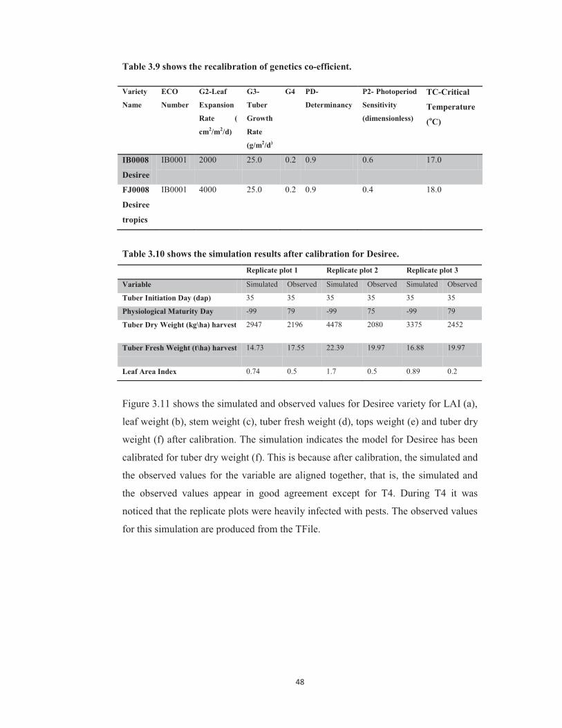
48
Table 3.9 shows the recalibration of genetics co-efficient.
Variety
Name
ECO
Number
G2-Leaf
Expansion
Rate (
cm2/m2/d)
G3-
Tuber
Growth
Rate
(g/m2/d)
G4 PD-
Determinancy
P2- Photoperiod
Sensitivity
(dimensionless)
TC-Critical
Temperature
(oC)
IB0008
Desiree
IB0001 2000 25.0 0.2 0.9 0.6 17.0
FJ0008
Desiree
tropics
IB0001 4000 25.0 0.2 0.9 0.4 18.0
Table 3.10 shows the simulation results after calibration for Desiree. Replicate plot 1 Replicate plot 2 Replicate plot 3
Variable Simulated Observed Simulated Observed Simulated Observed
Tuber Initiation Day (dap) 35 35 35 35 35 35
Physiological Maturity Day -99 79 -99 75 -99 79
Tuber Dry Weight (kg\ha) harvest 2947 2196 4478 2080 3375 2452
Tuber Fresh Weight (t\ha) harvest 14.73 17.55 22.39 19.97 16.88 19.97
Leaf Area Index 0.74 0.5 1.7 0.5 0.89 0.2
Figure 3.11 shows the simulated and observed values for Desiree variety for LAI (a),
leaf weight (b), stem weight (c), tuber fresh weight (d), tops weight (e) and tuber dry
weight (f) after calibration. The simulation indicates the model for Desiree has been
calibrated for tuber dry weight (f). This is because after calibration, the simulated and
the observed values for the variable are aligned together, that is, the simulated and
the observed values appear in good agreement except for T4. During T4 it was
noticed that the replicate plots were heavily infected with pests. The observed values
for this simulation are produced from the TFile.

49
Figure 3.11 shows the potential and observed calibration results for Desiree.
a) LAI b) Leaf weight
d) Stem weight c) Tuber fresh weight
e) Tops weight f) Tuber dry weight

50
Linear regression function was also calculated for tuber dry weight. The straight line
represents the linear regression function which relates the observed and simulated
tuber yield. The linear regression analysis helps to evaluate the model performance
by providing information on the slope (biasness) and the coefficient of determination
(R2), which provides information on how well the model (simulated values) agrees
with the observed values.
Figure 3.12 shows the evaluation of potato yield (dry matter in kg/ha) at Banisogosogo Fiji
for year 2012. The R2 for replicate plot 1 was 0.88 (y=1.62x-143.02), the R2 for replicate
plot 2 was 0.66 (y=0.99x+674.02) and the R2 for replicate plot 3 was 0.92 (y=1.11x+21.04).
The calibration of the DSSAT SUBSTOR Potato model gave a very close agreement
between the simulated and observed yields. The highest R2 value was for replicate
plot 3 (R2= 0.92) followed by replicate plot 1 (R2= 0.88) and replicate plot 2 (R2=
0.66) indicating a positive relationship between the simulated yield and the observed
yield. Replicate plot 2 had the lowest values for R2. As indicated by Table 3.7, the
value for T4 (2081 kg/ha) was much smaller than T3 value (4270 kg/ha). This may
be due to the impact of pests during T3 and T4. This gives rise to lower value of R2
for replicate plot 2.

51
3.3 Discussion
Trial and error field experiments approach for agrotechnology transfer is not only
time consuming but also costly. Hence, the use of system simulations and decision
support systems for agrotechnology transfer has been adopted and promoted (Singh
et al., 2002). The DSSAT SUBSTOR Potato model is site and cultivar specific.
Hence, before using the model in a new location, it has to be recalibrated (Singh et
al., 1998). The DSSAT SUBSTOR Potato model was calibrated by adapting soil
(water and nitrogen content), weather and management practises into model input
files. The tuber yield and the cultivar were used as evaluation parameters. This was
done to assess the accuracy and sensitivity of the model (Štastna and Dufkova,
2008).
Tables 3.2 and 3.3 show the chemical and physical properties of Banisogosogo soil.
Replicate plot 1 had the lowest pH (6.5-7.0) followed by replicate plot 2 (6.7-7.1)
and replicate plot 3 (6.8-7.2), while the highest organic carbon and nitrogen were
evident in replicate plot 2. The texture of the soil was clay. The optimum pH for
potato cultivation was 5.5-6.0 and the crop preferred high organic matter soils (Singh
et al., 1998).
The minimum weather data input required for the model are solar radiation (MJ
m2/d), maximum and minimum temperature (oC) and precipitation ( mm) (Rezzoug
et al., 2008). From the monthly average temperature of Banisogosogo (Table 3.5)
and the Weatherman Output of rainfall and temperature (Figure 3.8 and 3.9
respectively), the trend suggests that the highest solar radiation (19.4 MJ/m2/d, 18.7
MJ/m2/d and 19.4 MJ/m2/d), maximum temperature (30.6 oC, 30.2 oC and 31 oC),
minimum temperature (23.6 oC, 23.0 oC and 23.8 oC) and rainfall (990.4 mm, 460.5
mm and 761.3 mm) were received in the beginning of the year (January, February
and March respectively) while the lowest temperature (27.8 oC and 20.6 oC for
maximum temperature and minimum temperature respectively) and rainfall (18.6
mm) were recorded in July. Since the lowest average monthly temperature was
recorded in July (27.8 oC day/20.6 oC night), this indicates that July was a good time
for potato cultivation. Cool night temperatures are required by potatoes for
tuberisation. Ideal overnight temperatures are between 15-18 oC (Levy and Veilleux,

52
2007). The optimum amount of rainfall needed for potato cultivation was 50-75 cm
(Singh et al., 1998).
The soil water module used by DSSAT SUBSTOR Potato model is based on
Ritchie’s water balance model. The plant available soil water is determined from
drained upper limit and lower limit of plant extractable soil water for the given soil
(Ritchie, 1981a, b) and the nitrogen balance is simulated using the CERES N model
(Godwin and Singh, 1998) where at each growth stage of the crop, soil water or
nitrogen stress will affect the growth of the crop and hence the final yield (Knox et
al., 2010). The soil water content was recalculated and a nitrogen response
experiment was created to determine the amount of ammonia and nitrate in the soil.
The first calibration step involved adjusting the soil water content, that is, the
Drained Upper Limit (DUL), Lower Limit (LL), Soil Moisture Upper Limit
Saturated (SSAT) and Bulk Density (SDBM). This was manually recalculated using
a conversion factor from Default Medium Silty Clay. The algorithm used in SBuild
was unable to differentiate tropical soils with high clay content and aggregation due
to iron oxides as in Banisogosogo form the soil with similar clay content without
aggregation. Hence, Default Medium Silty Clay with similar water holding capacity
to the Banisogosogo soil was used to calculate a conversion factor for the new values
of bulk density, drained lower limit, drained upper limit and saturation (Table 3.4).
Likewise, AFile and TFile were also created under Experiment Data. AFile
represented the average values of the final harvest (T4) while the TFile represented
the average values of all the harvest, that is, T1, T2, T3 and T4. Table 3.6 of AFile
shows that the highest tuber dry weight (UWAD) was 2452 kg/ha which was
obtained from treatment 3 (replicate plot 3) and tuber fresh weight (UYAH) was
19.97 t/ha which was obtained from treatment 2 (replicate plot 2) and 3 (replicate
plot 3). Table 3.6 also indicates that treatment 3 gave the lowest leaf area index value
(LAIX) at harvest value of 0.2 and also by-product removed from harvest (BWAH)
at 970 kg/ha. On the other hand, TFile (Table 3.7) shows that the tuber fresh weight
starts to increase for each replicate plot from T2. T2 represents biomass partitioning
to competing organs or tubers. The partitioning to tubers is favoured by low
temperature, short photoperiod and low to moderate soil moisture and nitrogen
levels. In the DSSAT SUBSTOR Potato model the tubers are given the first priority

53
to accessible assimilate from photosynthesis and reserved carbohydrate pool. This
eliminates the need to directly estimate partitioning co-efficient to allocate carbon. In
non-limiting conditions, growth demands are met while in limiting conditions the
growth for leaves and vines are reduced and tubers are given the priority (Griffin et
al., 1993). It was also seen that LAI was the highest for T2 for each replicate plot
followed by a decline in T3 and T4. T2 is a stage where 90-100 % of the daily
acquired assimilates are partitioned to tubers. The length of T2 depends on the
relative tuber growth rate, which determines the rate of partitioning of dry matter
between the tubers and the rest of the plant (Haverkort, 2007a). The leaf weight
(except for leaf weight in replicate plot 1) and the stem weight were the highest for
T2 followed by a decline in T3. The model also assumes that the stem and leaves are
main sink for assimilates. However, as plants matures, majority of the assimilates are
transferred to the organ sinks (Singh et al., 1998). The tuber dry weight also
increased for T2 and T3 and declined for T4.
When simulation was conducted for the Desiree variety, it was seen that the
simulated values were not in agreement with the measured values (as shown by
Table 3.8 and Figure 3.10), for example, the simulated tuber initiation day was 50
days after planting while the measured tuber initiation day was 35 days after
planting. The genetic co-efficient of Desiree was recalibrated to Desiree-tropics to
achieve a match between the simulated and observed values of tuber initiation day,
tuber dry yield, tuber fresh yield and leaf area index. Under the genetic co-efficient
parameters, photoperiod sensitivity to tuber initiation is represented by P2 and the
critical temperature above which tuber initiation is inhibited is represented by TC
(oC). G2 (cm 2 m -2 d-1) represents leaf area expansion rate in degree days. G2 is
currently equivalent to 2000 cm 2 m -2 d-1 for all cultivars due to lack of evidence to
contrary. G3 (g m-2 d-1) is potential tuber growth rate. The level of determinacy of the
cultivar is defined by PD (Griffin et al., 1993). There was also notable difference
between the genetic co-efficient of Desiree and Desiree-tropics, that is, between the
original and the calibrated values, for example, changes were made to the leaf
expansion rate (G2) from 2000 cm2 m-2 d-1 to 4000 cm2 m-2 d-1, the value of
photoperiod was changed from 0.6 to 0.4 and the value for critical temperature (TC)
was changed from 17.0-18.0 oC (as shown by Table 3.9). After the calibration of the
genetic co-efficient, the simulated and the measured valued appeared much closer (as

54
shown in Table 3.10). The genetic co-efficient was derived iteratively through the
manipulation of the coefficient to achieve a match between the simulated and
observed values (Fraisse et al., 2001; Rezzoug et al., 2008). The cultivar parameters
were changed individually and the results were compared with the original and
previous run until the cultivar parameter modification gave the best output where the
simulated values matched the observed values. Formal sensitivity analysis was not
conducted in our evaluation but it was done directly in the Genetic Co-efficient file.
The reason for this is that when a formal Sensitivity Analysis was conducted, G2
values were not allowed to go beyond 3000 (maximum value), which shows that the
potato model, particularly the Desiree cultivar, has not been calibrated in the Tropic
regions. Hence, this calibration was done to suit the Tropical region and this brought
about marked improvement in the performance of the model. Most of the species
parameters are developed by modelers from experience of model calibration (Asadi
and Clemente, 2003) while some are developed from optimisation data sets (Gri mm
et al., 1993).
The calibration changes were associated with genetic co-efficient (specific to the
cultivar used) and soil parameters associated with the soil’s upper and lower limits.
The SUBSTOR Potato model subroutines and codes were not changed during the
calibration process. The adjustments to the genetic co-efficient are justified given the
Desiree variety has not been grown under temperature and daylength regime similar
to the experimental conditions. The lowered P2 value indicates greater photoperiod
sensitivity and the increased TC reflects higher temperature tolerance of Desiree
variety. These changes should not affect the performance of Desiree variety under
previously tested conditions. The higher G2 value in Table 3.9 used in the current
study requires verification and multi-location and trials. The simulated results show
that the differences are between the “calibrated” and the “original” model is
associated with changes in genetic co-efficient. The days for the tuber emergence and
harvest are identical; however, the changes are associated with the duration of the
tuber growth- 15 days longer for calibrated model. This combined with the LAI
effect led to higher tuber yield.
It is important for a crop model to accurately predict observed variation in yield,
before modelling climate impact on future yield. The DSSAT SUBSTOR Potato

55
model has been used internationally for crop studies and for climate change impact
studies (Knox et al., 2010). The DSSAT SUBSTOR Potato model has been tested in
various environments and has performed well when simulated data has been
compared with observed data (Bowen, 2003). However, such tests have been
conducted using only a few cultivars under temperate and subtropical/high altitude
environments. The DSSAT SUBSTOR Potato model was calibrated using data from
2012 season experimental replicate plot in Banisogosogo, Fiji. This allowed
comparison of model outputs to observed experimental results and field
measurements of the real system (Huang et al., 2009). Since replicate plot 2 had a
higher value of soil organic carbon content (Table 3.2), it simulated the highest tuber
dry yield (as shown by Table 3.10) and the simulation of replicate plot 2 by the
model also showed much more accuracy (that is, the simulated and the observed
values are much closer as indicated by Figure 3.11) as compared to the other
replicate plots. However, in the final harvest, the measured value of T4 (2080 kg/ha),
was not in good agreement with the simulated value (4478 kg/ha). This may be due
to the fact that during T3 and T4 harvest, the experimental replicate plot was heavily
infected with pest such as nematodes, beetle (Papuana spp.) and beetle larvae and
snail (Quantula striata) (Figures 3.5, 3.6 and 3.7). Due to the lack of disease or lack
of insect defoliation subroutines within the model (Griffin et al., 1993), the simulated
and measured values for T4 were not in agreement. The DSSAT SUBSTOR Potato
model was calibrated for tuber dry yield. The calibration results indicated that the
model is in good agreement with tuber dry weight. The DSSAT model has been
validated in Egypt and was successful in simulating current yield under different
irrigation levels and future yield under A1, A2, B1 and B2 for 2025, 2050, 2075 and
2100 (Medany, 2006). The model has also been validated for tuber initiation which
shows a strong linear relationship was apparent between simulated and observed data
for tuber initiation (Griffin et al., 1993). The model shows great potential for
simulating growth from experimental data (Singh et al., 1998). Since the model has
only been calibrated for tuber dry weight, the leaf area index was overestimated for
T1 and underestimated for T2, T3 and T4 (as shown by Figure 3.11). Leaf area index
is considered a key variable when calibrating models as it accounts for the leaf area
that intercepts the incoming radiation and it also takes part in major physiological
processes such as evapotranspiration, photosynthesis and biogenic emissions. High
LAI is important for potatoes for higher rates of tuber bulking for extended periods

56
which gives rise to higher yields (Geremew et al., 2008). In many crop monitoring
studies, in situ LAI have been used to calibrate crop models but the in situ LAI
measurements seemed inadequate as they are usually available for a limited number
of fields and dates (Gonzalez-Sanpedro et al., 2009). The DSSAT SUBSTOR Potato
model does not take into consideration the simulation of individual leaves but rather
the development of the entire canopy. The simulation of leaf growth is poorer than
the simulation of tuber initiation with a correlation co-efficient of 0.47. This model
tends to over-estimate the leaf area (Griffin et al., 1993; Fleisher et al., 2000). The
leaf weight, stem weight and the tuber fresh weight showed underestimation for T1
and T2 and overestimation for T3, and T4. Replicate plot 2 for top weight showed
different response when compared to all the other replicate plots. Replicate plot 2
was underestimated for T1 and T2 whereas overestimated for T3 and T4. Unlike
CERES-Maize model which has been extensively used in the Tropics (Singh et al.,
1990), the DSSAT SUBSTOR Potato model has been extensively tested in the
temperate regions. It is yet to be tested in the coastal regions, South-East Asia and
the Tropics (Singh et al., 1998).
Figure 3.12 shows the evaluation of potato yield (dry matter in kg/ha) at
Banisogosogo Fiji for the year 2012. The straight line represents the linear regression
function which relates the observed and simulated tuber yield and the coefficient of
determination (R2), which, assesses how well the shape of the simulation matches the
shape of the observed data (Knox et al., 2010). The highest R2 value is for replicate
plot 3 (R2= 0.92) followed by replicate plot 1 (R2= 0.88) and replicate plot 2 (R2=
0.66) indicating a positive relationship between the simulated yield and the observed
yield. It can also be said that each replicate plot is different. Replicate plot 2 has the
lowest values for R2. This might be due to factors not considered in the model, such
as, that of pest and disease (Griffin et al., 1993). As indicated by Table 3.7, the dry
matter (kg/ha) for replicate plot 2, the value for T4 (2081 kg/ha) is much smaller than
T3 value (4270 kg/ha) due to the impact of pests. This gives rise to lower value of R2
for replicate plot 2. Another difference highlighted by (Štastna and Dufkova, 2008) is
due to physiological difference projected into genetic parameters of the cultivar,
change in crop management and nutrient supply. In an experiment by (Štastna and
Dufkova, 2008), the validation for Rosara cultivar showed accuracy between
simulated and observed tuber yield (R2=0.97) while Karin showed lower value (R2=
57
0.43). The authors also stated that the use of model under extreme conditions, such
as, dry years showed that the model tend to underestimate tuber yield (Štastna and
Dufkova, 2008). This accurate simulation of tuber yield is critical as tuber yield are
not only economically important but is also affected by every process simulated in
the model, such as, the rate of development, intercepted radiation and use efficiency,
biomass partitioning, fertility and soil water status.
3.4 Recommendation
Several issues were identified for the usefulness and the improvement of the DSSAT
SUBSTOR Potato model. To begin with, further work is needed to test the DSSAT
SUBSTOR Potato model performance in the Tropics with vigorous multi-location
trials using suitable “tropical” varieties. The simulation of potato growth across the
diverse environment and different cultivars must also take into consideration the
effect of temperature, photoperiod and intercepted radiation. The application of the
model to a specific geographical location reduces the effectiveness of the model by
limiting the environmental inputs (Griffin et al., 1993).
Although the DSSAT SUBSTOR Potato model is now calibrated for tuber dry
weight, it is recommended that studies be conducted to further validate tuber weight,
LAI, leaf weight, stem weight and tuber weight under stress-free/minimal stress
conditions.
3.5 Experiment limitation
The following are the limitations of the experiment. Firstly, the soil water content
had to be manually recalculated using a conversion factor. The SBuild program
should be modified based on the soil data from the tropics. This also highlights the
need for actual measurement of the lower limit of plant extractable soil water and
drained upper limit under the field conditions for tropical soils.
The DSSAT SUBSTOR Potato model does not take into consideration the impact of
pest and disease on the tuber yield (Griffin et al., 1993). As indicated by the results,
T3 andT4 were badly affected by pests. More attention to pest and disease control is

58
needed for experimental trials, particularly those used for model validation since
most models do not simulate pest and disease effect.
Also, the DSSAT SUBSTOR Potato model does not read the year 2012 for the
measured data in PlantGro. The graph had to be exported to Excel and the Date had
to be manually changed from 2009 to 2012. Due to this, the Statics table did not give
any statistical value. It is recommended that the DSSAT SUBSTOR model should be
upgraded so that it is much easier to get the Statics whereby saving time.
The weather data imported into WeatherMan was also a combination of FMS and
NASA data. It was observed that the NASA values were slightly higher than the
FMS values. Investment in automated weather stations that determine daily solar
radiation, temperature, rainfall, humidity and wind would verify the quality of NASA
data.
Furthermore, the LAI was calculated during T1 using leaf area meter. However, from
T2-T4 the LAI was calculated using AccuPAR LP-80. Due to this, the model was not
calibrated for LAI.
59
Chapter 4 Simulation of Desiree potato variety growth and yield in three
different sites (Banisogosogo, Koronivia and Nacocolevu) in Fiji using the
calibrated DSSAT SUBSTOR Potato model
4.0 Introduction
Agricultural decision makers need increasing amount of information to meet
increasing demands for agricultural products and increased pressure on natural
resources for instance land and water (Jones et al., 2003). They also need to better
understand the possible outcomes of their decisions to assist them develop plans and
policies that meet their goals (Jones et al., 1998).
Many crop models have been used to study the growth and development of potatoes.
AquaCrop model has been used to study constraints limiting crop production and
water productivity in India. The model demonstrated good agreement between the
simulated and the observed values of belowground mass. However, the model proved
to be less satisfactory for aboveground mass and when simulating yield under high
water stress (Patel et al., 2008). An agrometeorological model was used to estimate
potential tuber yield in State of São Paulo, Brazil. The simulated and observed tuber
dry matter showed high correlation. However, the model underestimated the yield of
irrigated potato by less than 10 % (Pereira et al., 2008).
DSSAT has been developed to evaluate growth, production, resource use and the
risk linked with crop management practices (Jones et al., 1998). Crop models can
also be used to study variation in cultivar response to the environment (White, 1998).
The CERES crop model in DSSAT has been tested over a wide range of environment
and has also been used to simulate cereal crop growth and development with the
yields being within an acceptable limit of ±5 % to 15 % of measurable yields
(Ritchie et al., 1998).
The DSSAT SUBSTOR Potato model had been developed as a CERES-type model
and uses soil water and nitrogen dynamics that are used in other CERES type
models. The DSSAT SUBSTOR Potato model is successful in predicting potato
production (Abdrabbo et al., 2010) and has been tested in various environments with
good performance through comparison of simulated data with observed data (Bowen,
2003). The DSSAT SUBSTOR Potato model has a great potential to simulate potato
growth and evaluating possible changes in management in many regions (Griffin et

60
al., 1993). This model has also been validated in many areas and used to simulate
physiological processes and yield of potatoes under current climate and future
conditions (Bowen et al., 1998; International Potato Center, 1999; Fleisher et al.,
2003; Štastna and Dufkova, 2008; Abdrabbo et al., 2010; Knox et al., 2010). It has
also been extensively used internationally for crop studies and recently for climate
change impacts (Knox et al., 2010). The DSSAT SUBSTOR Potato model can be
used to simulate on a day-to-day basis the growth and development of the potato
crop using information on climate, soil, management and cultivar (Jones et al., 2003;
Knox et al., 2010). The SUBSTOR Potato model also has the ability to simulate
growth under potential conditions and non-potential (water limiting and water and
nitrogen limiting) conditions (Singh et al., 1998). It assumes that tuber initiation (T1)
is a function of daylength, temperature, water and nitrogen status in soil. Tuber
initiation by early cultivars are less sensitive to high temperatures and long daylength
as compared to late cultivars (Singh et al., 1998). The deficiency or excess of
nitrogen is based on above-ground tissue nitrogen concentrations. There is delay in
development under excess nitrogen conditions (Singh et al., 1998). The impact of
weather variability on a given management option can also be analysed by DSSAT
SUBSTOR Potato model by running the model with many years of weather data
(Bowen, 2003).
Application of crop models for simulating crop growth and yield play a crucial role
in addressing issues of food supply (yield forecasting) and also the risk associated
with weather variability (Thornton and Wilkens, 1998). Simulation models can also
be used as an educational tool for the understanding of biological processes (Ortiz,
1998). The model can also be used to enhance the use of resources for improved crop
production and profitability (Ritchie et al., 1998). This type of agronomic research
increases the productivity of farmers so that they can compete with the global market
and also helps protect the environment through the sustainable use of natural
resources (International Potato Center, 2006). There is a need to simulate potato
production in Fiji using current and historical weather data. This will lead to an
understanding of how current weather data and extreme events affect potato
production around Fiji. This Chapter presents the findings of simulating potato
growth in three sites around Fiji using the calibrated DSSAT SUBSTOR Potato
model. The use of DSSAT on the effect of climate variability on crop production
61
system is now considered part of decision support system in resource management
(United Nations, 2002). The impact of ENSO can also be studied in DSSAT through
multiple runs. These simulations can facilitate the task of optimising crop growth and
yield and suggesting recommendations on these crop management strategies.
Through these, policies and technologies can be identified that can take advantage of
positive opportunities or help in the reduction of adverse impacts of extreme weather
impacts. Also, improvements in forecast skills of ENSO can improve disaster
preparedness and improve production decisions of farmers (Valdivia et al., 2000).
4.1 Methodology
4.1.1 Simulation sites
The simulation sites for current climate included Banisogosogo, Koronivia and
Nacocolevu. Information on geographical location and reason for site selection for
Banisogosogo was provided in Chapter 3. Nacocolevu (also known as Sigatoka
Valley), is located between (18˚05'52.36" S, 177˚31'49.46" E). Sigatoka Valley is
located in Fiji’s western drier zone (Borrower, 2005). The western division is the dry
zone and is subjected to large seasonal and inter-annual climatic variation. Sigatoka
receives annual average to about 2000 mm. During the winter weather in these areas,
it is clear or partly cloudy with abundance of sunshine and a strong west to north-
westerly winds by day and south easterlies are prominent wind at night and in all
months except for August to March, the wind is mostly from north westerly quarter.
The nights are quite cool in this season. However, during summer there is
thunderstorm activity which is responsible for brief but intense rainfall (Gawander et
al., 2012). The average maximum temperature of Nacocolevu is 29.7oC while the
average minimum temperature is 21oC (Fiji Meteorological Services, 2013c)
The third site is Koronivia, in Nausori, which is located between (18˚03'00" S,
178˚32'00" E) (National Geospatial-Intelligence Agency, 2012a). Nausori is located
on the windward side of Viti Levu (Nausori Town Council, 2011). The climate
conditions of Nausori are often warm and humid. Nausori receives annual rainfall of
2000 mm annually while the higher range of Naitasiri receives an average rainfall of
6000 mm annually. During heavy rainfall, low lying areas of Rewa Delta are heavily
affected. The average temperature range of Nausori is from 28-30 oC. The cyclones
are normally confined to the wet season (Nausori Town Council, 2011).

62
4.1.2 Reason for site selection
Banisogosogo and Nacocolevu were selected for simulation purposes because these
are potato cultivating areas. Sigatoka Valley is considered the major center for potato
production at 134 hectares (Iqbal, 1982). The area also has soil which is suitable for
potato production (Autar, 2009; Macfarlane, 2009). Hence, simulation was
conducted to evaluate the impact of climate variability and to investigate how
growth, development and yield are affected by weather and soil of these areas.
Furthermore, Koronivia was selected as a simulation site to see if this site can be
considered as a potato cultivation area. It is also interesting because Koronivia is
located on the southern part of Viti Levu and also where Koronivia Agriculture
Research Station is located.
Figure 4.0 shows the location of three simulation sites. Source: (GoogleEarth, 2012).

63
4.1.3 Data collection, treatments and importations
4.1.3.1 Weather data
The 30 year climatic data for Penang (Banisogosogo), Koronivia and Nacocolevu,
such as, daily maximum temperature (oC), minimum temperature (oC) and
precipitation (mm) were collected from the Sugar Research Institute of Fiji (SRIF)
and Fiji Meteorological Services (FMS). Solar radiation of the experimental site was
also downloaded from NASA website. The weather data had missing values which
were replaced with NASA data creating a “hybrid” weather data. The DSSAT format
weather data was created in 2007 Excel worksheet. This Excel worksheet was then
imported into WeatherMan tool in DSSAT.
4.1.3.2 Soil data
As discussed in Chapter 3, soil samples of Banisogosogo were given to Koronivia
Research Station for analysis. The soil data of Koronivia and Nacocolevu were
recorded from secondary sources, that is, written reports which were provided by
Koronivia Research Station. Information on soil physical and chemical properties,
such as, colour, pH, nitrogen and organic carbon content, cation exchange capacity
(CEC) and base saturation for each layer was noted. These soil data were entered into
SBuild tool of DSSAT SUBSTOR Potato model.
4.1.3 Model simulation under current climatic and potential conditions
The calibrated DSSAT SUBSTOR Potato model (from Chapter 3) was used to create
potential and non-potential simulations for Banisogosogo, Koronivia and
Nacocolevu. The simulations were created using site specific current weather
conditions and soil physical and chemical information. Banisogosogo simulation was
conducted with available weather and soil data, that is, weather data of 1960-2012,
with Banisogosogo Replica 2 soil using the calibrated DSSAT SUBSTOR Potato
model. Koronivia potential and non-potential simulations were run using weather
data from 1961-2010 with Koronivia Silt Loam Soil. Nacocolevu potential and non-
potential simulations were conducted using weather data from July 1972-2010 with
Nacocolevu Rolling Phase Soil.
The crop management practices used was the same as in Chapter 3. The date of
irrigation application, the amount of irrigation application and the method of

64
application were similar in all sites. There were four irrigation applications using
Drip or Trickle method. Fertiliser amount of 80 N kg/ha was applied in 2 splits.
Similar fertiliser application techniques were used for all the sites. This information
is summarised in Table 4.0, Table 4.1 and Table 4.2. For potential simulations, the
model assumed that there was no water or nitrogen stress and that the plant was
grown under perfect conditions while non-potential simulation assumed that there
was water and nitrogen stress.
Table 4.0 shows the summary of simulations at Banisogosogo, Koronivia and
Nacocolevu.
Site Banisogosogo Koronivia Nacocolevu
Soil Name Banisogosogo Replica 2
Soil
Koronivia Silt Loam Nacocolevu Soil,
Rolling Phase
Weather Station Penang Nausori Nacocolevu
Cultivar Desiree Desiree Desiree
Planting Date 2nd July 2nd July 2nd July
Planting Method Dry seed Dry seed Dry seed
Planting Distribution Rows Rows Rows
Plant Population
(seedling) (m2)
5 5 5
Row Spacing ( cm) 75 75 75
Planting Depth ( cm) 1.5 1.5 1.5
CO2 Concentration Actual CO2, Mauna
Loa, Hawaii
Actual CO2, Mauna
Loa, Hawaii
Actual CO2, Mauna
Loa, Hawaii

65
Table 4.1 shows the irrigation application during simulations at Banisogosogo,
Koronivia and Nacocolevu.
Site Date (dd/ mm/yyyy) Irrigation ( mm) Operation
Banisogosogo,
Koronivia, Nacocolevu
02/07/2012
13/07/2012
05/08/2012
10/09/2012
1.6
4
4
4
Drip or Trickle
Drip or Trickle
Drip or Trickle
Drip or Trickle
Table 4.2 shows the fertiliser application during simulations at Banisogosogo,
Koronivia and Nacocolevu.
Site Date (dd/
mm/yyyy)
Fetriliser
Material
Fertiliser Application Depth
( cm)
N
Amount
(kg/ha)
Banisogosogo,
Koronivia,
Nacocolevu
02/07/2012
23/07/2012
Diammonium
phosphate
Diammonium
phosphate
Banded beneath
surface
Banded beneath
surface
5
5
40
40
4.1.4 Optimisation treatment through sensitivity analysis
The optimisation treatments were simulated for planting time, row spacing, irrigation
treatment, fertiliser treatment and planting depth to optimise potato yield at each
simulation site using the DOS method in Sensitivity Analysis in DSSAT SUBSTOR
Potato model. The weather data of 2012 was used for all optimisation treatments
(except planting time) for Banisogosogo non-potential simulation with 2nd July 2012
as default run. The optimisation treatments (except planting time) for Koronivia and
Nacocolevu non-potential simulations were run with 2010 weather data with 2nd July
2010 as default run. The planting times for all three sites were simulated with 2009
weather data with 2nd July 2009 as default run. When using 2010 weather data for
optimisation of planting date, it was noted that there were no yield for October,

66
November and December as 2011 weather data was not available. It was assumed
that the crop will be harvested in 90 days. Hence, this optimisation treatment was
conducted with 2009 weather data.
In this simulation, all other crop management details remained the same except for
the optimisation treatment. The optimisation for planting time was simulated on the
first day of the month (except for January which was carried out on the 2nd of
January due to the start of simulation date which needs to be before the planting
date). It was assumed that the harvest day was 90 days after planting. The
optimisations for row spacing were simulated at 30 cm, 40 cm, 50 cm, 80 cm and
100 cm with 75 cm as a default run. For irrigation and fertiliser optimisation, water
and nitrogen stress days were recorded from initial non-potential simulation. The
irrigation optimisations were simulated on a fortnightly basis and three days before
water stress from non-potential simulation. The irrigation treatments were at 1.6 mm,
4.0 mm, 6.4 mm, 8.0 mm, 9.6 mm, 12.0 mm, 14.0 mm, and 16.0 mm with default run
as 1.4 mm and 6.0 mm (refer to Table 4.1). The fertiliser optimisation was carried
out from 60 N kg/ha to 300 N kg/ha at 60 N kg/ha interval (this was applied in 3
splits, one on the day of planting and the other 2 splits were simulated 3 days before
the nitrogen stress from non-potential simulation) with default run as 80 N kg/ha
applied in 2 splits at 5 cm (Table 4.2). The optimisation for planting depth was also
conducted from 2 cm to 10 cm at interval of 2 cm with default run of 1.5 cm. Finally,
the optimum application of fertiliser and irrigation from the fertiliser and irrigation
simulations were noted and these treatments were also simulated together to see if
the yield was optimised.
4.1.5 Climate variability (El Niño Southern Oscillation)
The impact of climate variability, El Niño Southern Oscillation (ENSO) state, on
potato yield in Fiji was also studied. To conduct the simulation for ENSO years, for
the Simulation Options, under General tab, the number of years were changed to
make the model run for that number of years. Banisogosogo simulation was
conducted from 1983-2012 while Koronivia and Nacocolevu simulation was
conducted from 1990-2010. The Fiji Meteorological Services helped to identify the
ENSO state from 1983-2012. The percentage difference was also calculated with
neutral year as a baseline.
67
4.1.6 Data analysis
The above inputs (soil data, weather data and crop management data) were used to
run simulation for the three locations. All summary outputs, graphical and initial
analysis were done in DSSAT v4.5 Output. Other statistical analysis was conducted
in Microsoft 2007 Excel Spreadsheet. These outputs are presented in the Results
section.
4.2 Results
This section describes the simulation of Desiree potato variety growth and yield
under current climate conditions in three different sites, that is, Banisogosogo,
Koronivia and Nacocolevu using the calibrated DSSAT SUBSTOR Potato Model.
The simulations were conducted with the site specific soil data, site specific weather
data and crop management practices. Under potential simulation, Koronivia gives the
highest tuber yield while Nacocolevu gave the highest tuber yield under non-
potential simulation. The impact of climate variability, ENSO state, was also studied
on potato yield for the three locations. Differences in the yield were noticed for
ENSO simulation for the three locations due to differences in weather data and the
water and nitrogen stress faced under El Niño, La Niña and neutral years. In addition
to these, optimisation treatments also investigated which crop management practices,
such as planting date, row spacing, irrigation treatment, fertiliser treatment, optimum
irrigation and optimum fertiliser treatment and planting depth can optimise potato
yield.
4.2.1 Weather data
Site specific “hybrid” weather data for Banisogosogo, Koronivia and Nacocolevu
was imported into WeatherMan tool in DSSAT. The monthly averages for the three
sites indicated that the potato growing season (July-September) received lower
values of average monthly maximum temperature, minimum temperature and rainfall
as compared to months earlier than the potato growing season and later than the
potato growing season (Figures 4.1 and 4.2 and Table 4.3).

68
Figure 4.1 shows the monthly average rainfall for Banisogosogo, Koronivia and Nacocolevu.
Figure 4.2 shows the monthly average maximum and minimum temperature for
Banisogosogo, Koronivia and Nacocolevu.

69
Table 4.3 shows the average monthly maximum temperature, minimum temperature
and rainfall for Banisogosogo, Koronivia and Nacocolevu.
Banisogosogo Koronivia Nacocolevu
Tmax
(oC)
Tmin
(oC)
Rainfall
( mm)
Tmax (oC) Tmin (oC) Rainfall
( mm)
Tmax
(oC)
Tmin
(oC)
Rainfall
( mm)
January 30.4 23.9 409.6 30.3 23.2 354.8 31.3 22.3 174.5
February 30.5 23.8 361.7 30.7 23.4 272.5 31.5 22.7 156.8
March 30.5 23.7 411.7 30.4 23.2 369.8 31.3 22.7 157.4
April 29.7 23.3 302.1 29.4 22.6 343.5 30.5 21.7 160.5
May 28.7 22.3 146.9 28 21.3 228.3 29.3 20 153.9
June 28.1 21.6 99.9 27.3 20.7 163.9 28.5 18.9 152.8
July 27.6 20.7 52.1 26.4 20.0 136.1 27.5 17.9 162.6
August 27.8 20.9 74.3 26.4 19.9 147.7 27.6 17.9 184.5
September 28.4 21.5 101.3 26.8 20.4 174.9 28 18.5 170.7
October 29 22.3 104.4 27.7 21.1 214.5 29.2 19.6 200.1
November 29.7 23 173.6 28.7 21.9 249.8 30.4 20.9 185
December 30.2 23.5 272.9 29.6 22.6 277.2 31.1 21.7 181
Annual Average 29.2 22.54 209.21 28.47 21.69 244.41 29.68 20.4 169.98
Season Average 27.93 21.03 75.9 26.53 20.1 152.9 27.7 18.1 147.48
4.2.2 Simulation results for Desiree
The current climate simulations were conducted for Banisogosogo, Koronivia and
Nacocolevu using Desiree variety. The simulations were run using site-specific soil
data, site-specific weather data and crop management practices. The results indicated
that the potential yield is higher than the non-potential yield. The potential tuber dry
weight for Banisogosogo was 6651 kg/ha while the non-potential tuber dry weight
was 4478 kg/ha. Koronivia simulation indicated that the potential tuber dry weight
was 9811 kg/ha but the non-potential tuber dry was 4373 kg/ha. Under Nacocolevu
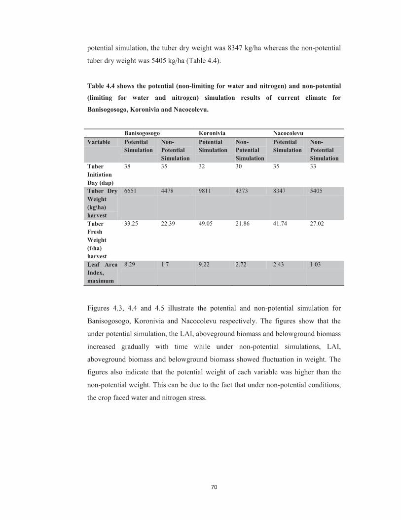
70
potential simulation, the tuber dry weight was 8347 kg/ha whereas the non-potential
tuber dry weight was 5405 kg/ha (Table 4.4).
Table 4.4 shows the potential (non-limiting for water and nitrogen) and non-potential
(limiting for water and nitrogen) simulation results of current climate for
Banisogosogo, Koronivia and Nacocolevu.
Banisogosogo Koronivia Nacocolevu Variable Potential
Simulation Non-Potential Simulation
Potential Simulation
Non-Potential Simulation
Potential Simulation
Non-Potential Simulation
Tuber Initiation Day (dap)
38 35 32 30 35 33
Tuber Dry Weight (kg\ha) harvest
6651 4478 9811 4373 8347 5405
Tuber Fresh Weight (t\ha) harvest
33.25 22.39 49.05 21.86 41.74 27.02
Leaf Area Index, maximum
8.29 1.7 9.22 2.72 2.43 1.03
Figures 4.3, 4.4 and 4.5 illustrate the potential and non-potential simulation for
Banisogosogo, Koronivia and Nacocolevu respectively. The figures show that the
under potential simulation, the LAI, aboveground biomass and belowground biomass
increased gradually with time while under non-potential simulations, LAI,
aboveground biomass and belowground biomass showed fluctuation in weight. The
figures also indicate that the potential weight of each variable was higher than the
non-potential weight. This can be due to the fact that under non-potential conditions,
the crop faced water and nitrogen stress.

71
Figure 4.3 shows Banisogosogo potential and non-potential simulations for stem weight,
LAI, tuber fresh weight, leaf weight, tops weight and tuber dry weight.
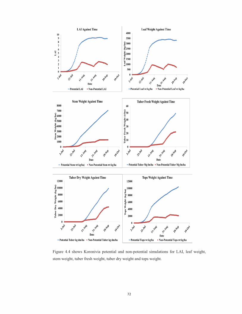
72
Figure 4.4 shows Koronivia potential and non-potential simulations for LAI, leaf weight,
stem weight, tuber fresh weight, tuber dry weight and tops weight.

73
Figure 4.5 shows Nacocolevu potential and non-potential simulations for LAI, leaf weight,
stem weight, tuber fresh weight, tuber dry weight and tops weight.

74
Impact of precipitation, total water content of the soil, nitrate content of the soil and
nitrogen leached from the soil were also studied on non-potential tuber dry weight
and LAI for Banisogosogo (Figure 4.6), Koronivia (Figure 4.7) and Nacocolevu
(Figure 4.8).
Figure 4.6 shows the impact of precipitation, total water and nitrogen content in soil on non-
potential tuber dry yield and LAI for Desiree in Banisogosogo over the growing season.
The Banisogosogo simulation (Figure 4.6) indicated that upon application of nitrogen
fertiliser, the nitrate level in the soil increased. The figure shows that LAI (a) started
to increase a few days after planting (9th of July). The LAI reached its maximum
(1.7) around 20th of August and 26th of September. The LAI decreased around 20th of
a) LAI
b) Tuber dry weight

75
August. Around the same time the tuber dry weight (b) started to increase gradually
until the harvest day.
Figure 4.7 shows the impact of precipitation, total water and nitrogen content in soil on non-
potential tuber dry yield and LAI for Desiree in Koronivia over the growing season.
For Koronivia simulation (Figure 4.7), it was seen that precipitation levels increased
gradually and around 30th August when the precipitation levels were high and the
nitrate levels decreased in the soil. The LAI (a) showed fluctuation over the growing
season with the maximum LAI (2.5 and 2.72) being achieved on 9th of August and 5th
of September respectively. The tuber dry weight (b) increased when the LAI dropped
the first time (10th of August) and it continued to increase gradually until the 30th of
a) LAI
b) Tuber dry weight

76
August, however, a sharp increase in tuber dry weight occurred after 30th of August.
The figure also shows the trend for total nitrate and water in the soil.
Figure 4.8 shows the impact of precipitation, total water and nitrogen content in soil on non-
potential tuber dry yield and LAI for Desiree in Nacocolevu over the growing season.
Figure 4.8 illustrates that Nacocolevu water content was consistent throughout the
planting season. The precipitation increased gradually over time and the figure also
indicated that the total nitrate leached from the soil also increased gradually over
time. The LAI (a) increased steadily until the 17th of August where the maximum
a) LAI
b) Tuber dry weight

77
LAI was attained at 1. After the 7th of August the LAI decreased. On the other hand,
the tuber dry weight (b) increased steadily over time. The figure shows that the total
water content in the soil was consistent over time with some nitrogen leaching
experienced as precipitation increased.
4.2.3 Optimisation treatments
The optimisation simulations were conducted to investigate which crop management
option maximised tuber yield. The optimisation simulation was conducted for
planting time, row spacing, irrigation treatment, fertiliser treatment, optimum
fertiliser and optimum irrigation treatment and also planting depth. In general, the
results indicated that different crop management strategies maximised yield in
different locations.
Table 4.5 shows the optimum planting time for Desiree variety for Banisogosogo,
Koronivia and Nacocolevu. The optimum planting time for Banisogosogo was May
while the optimum planting time for Koronivia and Nacocolevu was August.
Table 4.5 shows the yield at different planting time for Banisogosogo, Koronivia and
Nacocolevu.
Yield (kg/ha)
Planting Time Banisogosogo Koronivia Nacocolevu
January 2 18 395 63
February 1 13 607 208
March 1 289 2223 1444
April 1 2109 4117 4006
May 1 5356 1959 1280
June 1 4567 4103 1135
July 2 (default run) 3698 6703 4823
August 1 4329 7956 7612
September 1 967 3824 5899
October 1 2523 7384 3375
November 1 316 2088 3197
December 1 179 1137 234
The table below (Table 4.6) shows the optimum row spacing for Desiree variety for
Banisogosogo, Koronivia and Nacocolevu. The optimisation for row spacing was
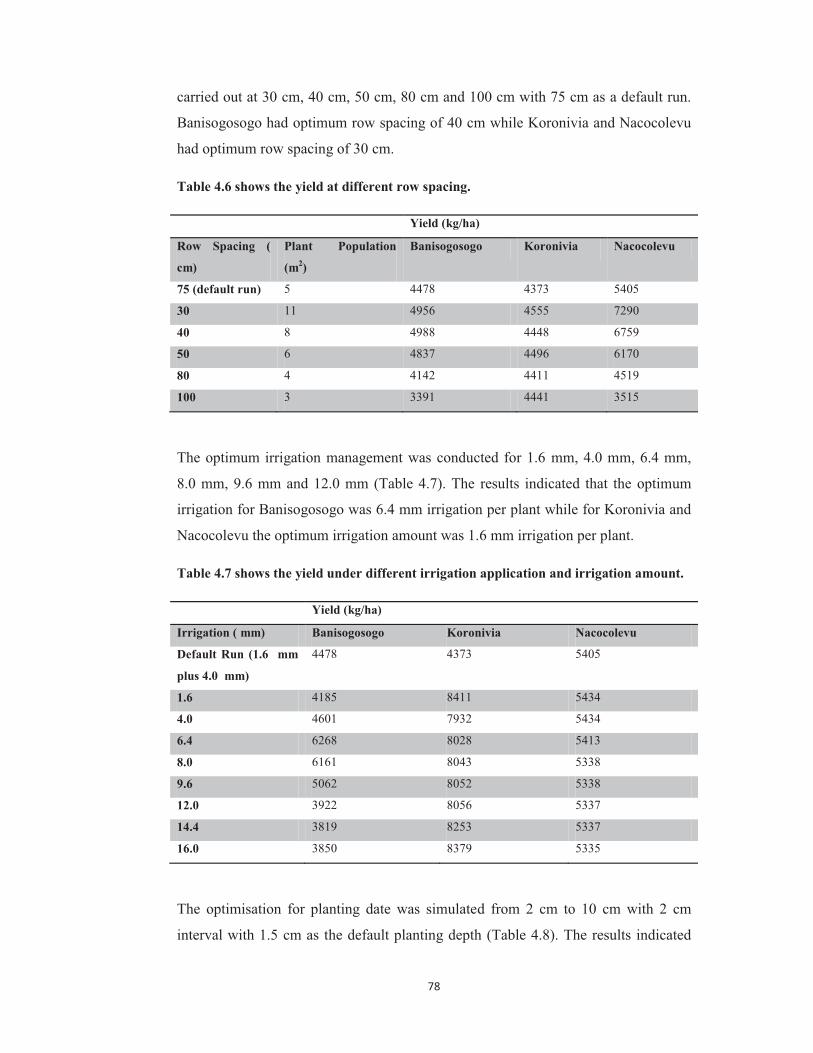
78
carried out at 30 cm, 40 cm, 50 cm, 80 cm and 100 cm with 75 cm as a default run.
Banisogosogo had optimum row spacing of 40 cm while Koronivia and Nacocolevu
had optimum row spacing of 30 cm.
Table 4.6 shows the yield at different row spacing.
Yield (kg/ha)
Row Spacing (
cm)
Plant Population
(m2)
Banisogosogo Koronivia Nacocolevu
75 (default run) 5 4478 4373 5405
30 11 4956 4555 7290
40 8 4988 4448 6759
50 6 4837 4496 6170
80 4 4142 4411 4519
100 3 3391 4441 3515
The optimum irrigation management was conducted for 1.6 mm, 4.0 mm, 6.4 mm,
8.0 mm, 9.6 mm and 12.0 mm (Table 4.7). The results indicated that the optimum
irrigation for Banisogosogo was 6.4 mm irrigation per plant while for Koronivia and
Nacocolevu the optimum irrigation amount was 1.6 mm irrigation per plant.
Table 4.7 shows the yield under different irrigation application and irrigation amount.
Yield (kg/ha)
Irrigation ( mm) Banisogosogo Koronivia Nacocolevu
Default Run (1.6 mm
plus 4.0 mm)
4478 4373 5405
1.6 4185 8411 5434
4.0 4601 7932 5434
6.4 6268 8028 5413
8.0 6161 8043 5338
9.6 5062 8052 5338
12.0 3922 8056 5337
14.4 3819 8253 5337
16.0 3850 8379 5335
The optimisation for planting date was simulated from 2 cm to 10 cm with 2 cm
interval with 1.5 cm as the default planting depth (Table 4.8). The results indicated
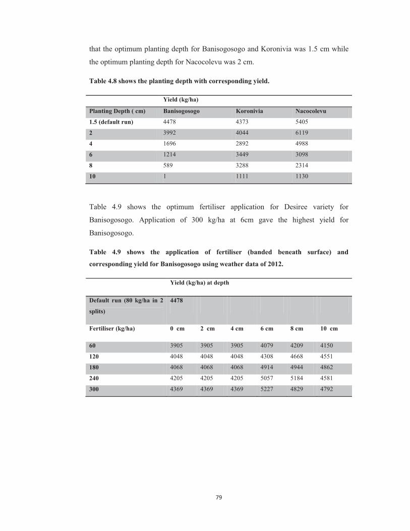
79
that the optimum planting depth for Banisogosogo and Koronivia was 1.5 cm while
the optimum planting depth for Nacocolevu was 2 cm.
Table 4.8 shows the planting depth with corresponding yield.
Yield (kg/ha)
Planting Depth ( cm) Banisogosogo Koronivia Nacocolevu
1.5 (default run) 4478 4373 5405
2 3992 4044 6119
4 1696 2892 4988
6 1214 3449 3098
8 589 3288 2314
10 1 1111 1130
Table 4.9 shows the optimum fertiliser application for Desiree variety for
Banisogosogo. Application of 300 kg/ha at 6cm gave the highest yield for
Banisogosogo.
Table 4.9 shows the application of fertiliser (banded beneath surface) and
corresponding yield for Banisogosogo using weather data of 2012.
Yield (kg/ha) at depth
Default run (80 kg/ha in 2
splits)
4478
Fertiliser (kg/ha) 0 cm 2 cm 4 cm 6 cm 8 cm 10 cm
60 3905 3905 3905 4079 4209 4150
120 4048 4048 4048 4308 4668 4551
180 4068 4068 4068 4914 4944 4862
240 4205 4205 4205 5057 5184 4581
300 4369 4369 4369 5227 4829 4792

80
Table 4.10 shows that the yield is higher than default run and fertiliser optimisation
yield but not higher than irrigation yield.
Table 4.10 shows the optimum fertiliser and irrigation management simulation for
Banisogosogo using weather data of 2012.
Optimum Fertiliser and Irrigation Management
Fertiliser Application (kg/ha at 6 cm) Irrigation Application ( mm) Yield (kg/ha)
300 kg/ha 6.4 mm 5719
The optimum fertiliser application for Desiree variety for Koronivia indicated that
application of 300 kg/ha at 6 cm gave the highest yield for Koronivia (Table 4.11).
Table 4.12 indicated that the yield was higher than default run and fertiliser
optimisation yield but not higher than irrigation yield.
Table 4.11 shows the application of fertiliser (banded beneath surface) and
corresponding yield for Koronivia using weather data of 2010.
Yield (kg/ha) at depth
Default run (80 kg/ha in 2
splits at 5 cm)
4373
Fertiliser (kg/ha) 0 cm 2 cm 4 cm 6 cm 8 cm 10 cm
60 3987 3987 3987 3972 3989 3987
120 3792 3792 3792 3705 4038 4080
180 4037 4037 4037 3840 3796 3768
240 4406 4406 4406 4144 4344 4368
300 4426 4426 4426 4389 4398 4564
Table 4.12 shows the corresponding yield of optimum fertiliser and irrigation
management for Koronivia using weather data of 2010.
Fertiliser Application (kg/ha at
10 cm)
Irrigation Application ( mm) Yield (kg/ha)
300 kg/ha 1.6 4602

81
For Nacocolevu, application of 300 kg/ha at 10 cm gave the highest yield (Table
4.13). The results obtained also indicated that higher yield was obtained under
optimum fertiliser and optimum irrigation treatment (Table 4.14).
Table 4.13 shows the application of fertiliser (banded beneath surface) and
corresponding yield for Nacocolevu using weather data of 2010.
Yield (kg/ha) at depth
Default run (80 kg/ha in 2
splits)
5405
Fertiliser (kg/ha) 0 cm 2 cm 4 cm 6 cm 8 cm 10 cm
60 2594 2594 2594 2741 2922 3038
120 5036 5036 5036 5295 5551 5659
180 7077 7077 7077 6666 7597 7657
240 7393 7393 7393 7519 7650 7690
300 7649 7649 7649 7801 7895 7925
Table 4.14 shows the corresponding yield of optimum fertiliser and irrigation
management for Nacocolevu using weather data of 2010.
Fertiliser Application (kg/ha
at 10 cm)
Irrigation Application ( mm) Yield (kg/ha)
300 kg/ha 1.6 8343
300 kg/ha 4.0 8344
4.2.4 Climate variability (El Niño Southern Oscillation) simulation
The impact of climate variability was also studied on potato yield for the three
locations. Differences in the yield were noticed due to differences in weather data
and the water and nitrogen stress faced under El Niño, La Niña and neutral years for
the three locations. Under Banisogosogo and Nacocolevu simulation, neutral year
received the highest average yield (Tables 4.16, 4.20) while under Koronivia
simulation, El Niño received the highest average yield (Table 4.18).

82
Table 4.15 shows the impact of ENSO on potato yield for non-potential Banisogosogo
simulation from 1983-2012.
El
Niño
Water
Stress
N
Stress
Yield
(kg/ha)
La
Niña
Water
Stress
N
Stress
Yield
(kg/ha)
Neutral Water
Stress
N
Stress
Yield
(kg/ha)
1987 0.62 1.24 2129 1988 0.89 0.40 627 1983 - 0.06 6885
1991 0.15 0.28 779 1996 0.49 0.13 2846 1984 0.45 0.30 3216
1992 0.55 0.23 1934 1998 0.63 0.32 747 1985 0.30 0.14 3816
1993 0.09 0.09 473 1999 0.04 0.07 5500 1986 0.35 0.19 2362
1994 0.08 0.34 957 2000 0.22 0.16 4591 1989 0.33 0.15 5147
1997 0.08 0.21 826 2008 0.61 0.39 1465 1990 0.12 0.16 6179
2002 - 0.07 7744 2012 0.35 0.16 3816 1995 1.05 0.46 642
2004 0.07 0.08 5799 2001 0.58 0.20 3011
2006 0.48 0.10 3692 2003 0.46 0.25 816
2010 0.66 0.28 1407 2005 0.39 0.19 2514
2007 0.8 0.25 766
2009 0.23 0.36 2687
Table 4.16 indicates 7 year average for ENSO yield in Banisogosogo. The results
indicated that highest average yield was obtained under neutral year, with El Niño
giving a percentage difference of 61.4 % while La Niña gave a percentage difference
of 13.88 %.
Table 4.16 shows the 7 year average for ENSO yield for Banisogosogo.
7 Year Average Yield (kg/ha) Percentage Difference (%)
El Niño (1987-2002) 1868.71 61.4
La Niña (1988-2012) 3070 13.88
Neutral Year (1983- 1995) 3527.85

83
Table 4.17 shows the impact of ENSO on potato yield for non-potential Koronivia
simulation from 1990 to 2010.
El
Niño
Water
Stress
N
Stress
Yield La
Niña
Water
Stress
N
Stress
Yield Neutral Water
Stress
N
Stress
Yield
1991 0.41 0.39 6487 1996 0.69 0.18 1651 1990 0.18 0.31 5911
1992 0.58 0.18 4497 1998 0.98 0.12 757 1995 0.45 0.29 3837
1993 0.55 0.21 2056 1999 0.03 0.45 3754 2001 0.45 0.20 5147
1994 0.78 0.34 2709 2000 0.06 0.47 4188 2003 0.75 0.12 3857
1997 0.30 0.42 6577 2008 0.63 0.21 5284 2005 0.50 0.18 2691
2002 0.21 0.38 6107 2007 - - 3964
2004 0.07 0.49 5330 2009 0.46 0.23 5532
2006 0.56 0.23 6257
2010 0.93 0.55 4424
For 5 year average for ENSO yield in Koronivia, the results indicated that highest
average yield was obtained under El Niño at 4465.2 kg/ha with the lowest yield in La
Niña at 3126.8 kg/ha (Table 4.18).
Table 4.18 shows the 5 Year average for ENSO yield for Koronivia.
5 Year Average Yield (kg/ha) Percentage Difference
(%)
El Niño (1991-1997) 4465.2 -4.17
La Niña (1996-2008) 3126.8 31.19
Neutral Year (1990-2005) 4282.6
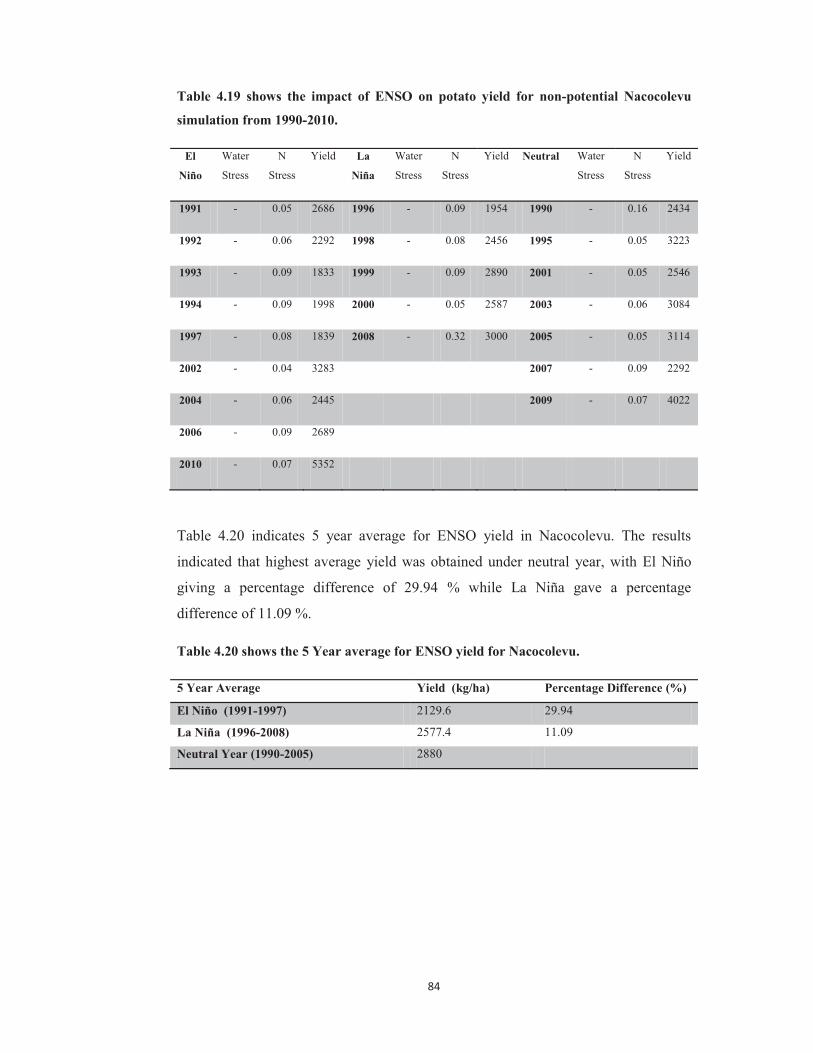
84
Table 4.19 shows the impact of ENSO on potato yield for non-potential Nacocolevu
simulation from 1990-2010.
El
Niño
Water
Stress
N
Stress
Yield La
Niña
Water
Stress
N
Stress
Yield Neutral Water
Stress
N
Stress
Yield
1991 - 0.05 2686 1996 - 0.09 1954 1990 - 0.16 2434
1992 - 0.06 2292 1998 - 0.08 2456 1995 - 0.05 3223
1993 - 0.09 1833 1999 - 0.09 2890 2001 - 0.05 2546
1994 - 0.09 1998 2000 - 0.05 2587 2003 - 0.06 3084
1997 - 0.08 1839 2008 - 0.32 3000 2005 - 0.05 3114
2002 - 0.04 3283 2007 - 0.09 2292
2004 - 0.06 2445 2009 - 0.07 4022
2006 - 0.09 2689
2010 - 0.07 5352
Table 4.20 indicates 5 year average for ENSO yield in Nacocolevu. The results
indicated that highest average yield was obtained under neutral year, with El Niño
giving a percentage difference of 29.94 % while La Niña gave a percentage
difference of 11.09 %.
Table 4.20 shows the 5 Year average for ENSO yield for Nacocolevu.
5 Year Average Yield (kg/ha) Percentage Difference (%)
El Niño (1991-1997) 2129.6 29.94
La Niña (1996-2008) 2577.4 11.09
Neutral Year (1990-2005) 2880

85
4.3 Discussion
4.3.1 Desiree potential simulation
The potential simulation showed a higher tuber fresh yield, tuber dry yield and LAI
as compared to non-potential simulation for the three areas (Table 4.4). Under
potential simulation, the model assumed that there was no water and nitrogen stress
on the growth and development stages of the plant (refer to Appendix 2A, Table
2.5A, Table 2.6 A, Table 2.9A and 2.10A, Table 2.13A and Table 2.14A). However,
the tuber initiation day (days after planting) for potential simulation occurred after
the non-potential simulation. The model also showed that potato grown in three
location simulated different yield. One reason for the difference in tuber yield for the
three sites can be the soil status and the weather for each site. It was also noticed that
when the aboveground weight (LAI, leaf weight, tops weight and the stem weight)
decreased, the belowground weight (tuber weight) started to increase around the
same time (Figures 4.3, 4.4 and 4.5). This can be due to all the carbohydrates being
partitioned to tuber growth following tuber initiation (Fleisher et al., 2003).
4.3.2 Desiree non-potential simulation
The Banisogosogo non-potential simulation indicated the tuber initiation day was 35
days after planting. The simulated tuber dry weight was 4478 kg/ha and tuber fresh
weight of 22.39 t/ha. The results also indicated that the maximum LAI was 1.7
(Table 4.4). The emergence date was 6th of July which was 7 days after planting
(Appendix 2A, Table 2.7A). The tuber forms around the 9th of August, which was 35
days after planting. The crop was harvested after 80 days, that was, on 20th of
September (Appendix 2A, Table 2.7A). Figure 4.3 and 4.6 indicated that from the
planting date (2nd of July) the LAI increased around the 10th of August. From the
planting day until 10th of August, the LAI, leaf weight, stem weight and tops weight
increased in value. After 10th August to 19th of September, the LAI, leaf weight, stem
weight and tops weight started to decrease while the tuber dry weight started to
gradually increase from 10th of August to 30th of August. From 30th of August to 19th
September there was a sharp increase in the tuber dry weight. The precipitation
increased around 30th of August which also increased the total water content in the
soil. Figure 4.6 also showed an increase in total nitrate rate over time. This can be
due to application of nitrogen fertilisers (on 7th and 23rd of July nitrogen fertiliser was

86
applied which also shows an increase in nitrate rate). The decrease in LAI can be
linked to transfer of photosynthate from the aboveground to the belowground. This
affected the LAI and other aboveground components such as leaf weight and tops
weight. The average leaf area or the ability to maintain complete soil cover by the
canopy during the growing season affects the tuber yield (Boyd et al., 2002). The
stem and leaves are main sink for assimilates. However, as plants mature, these
assimilate are relocated to the organ sinks (Dwelle and Love, 1993; Singh et al.,
1998), in this case the potato tubers. Table 4.3 indicated that the Banisogosogo had
the highest average maximum and minimum temperature for the growing season at
27.93 oC and 21.03 oC respectively with minimum rainfall at 75.9 mm for the
growing season. In tropical highlands, potato production is suitable under
temperature range of 15-18 ºC (Haverkort, 1990) or around 22 ºC (Burton, 1981).
The carbon assimilation and water use efficiency range of potatoes is between 16˚C-
25ºC and the optimal temperature for net photosynthesis at 25 ºC (Ku et al., 1977). In
lowland tropics, the potential yields of potato tubers are highest at daylength less
than 12 hours and average temperature of 20-23˚C (Zaag et al., 1986; Jackson,
1999). For cultivar Desiree, there was an increase in tuber number between the
temperature ranges of 15-23 ºC. Under temperatures of 2 oC and above 30 oC, the
growth and development of potatoes is not possible (Garner and Blake, 1989;
Haverkort, 2007a). The ideal soil temperature for tuber development is around 15oC-
18oC (Levy and Veilleux, 2007). Leaf appearance shows optimal values at an
average daily temperature of about 28 oC (Fleisher et al., 2006a). Regardless of night
temperature, the rate of leaf appearance peaks at 20 oC (Vos, 1995). High
temperatures gave higher specific leaf area as compared to the cool temperatures
(Midmore and Prange, 1991). The optimum temperature is also dependent on
photoperiod (Wheeler, 2006). Kennebec cultivar had a leaf area with a quadratic
relationship with temperature with the largest area at 16.6 oC and 22.1 oC. Main-stem
leaves accounted for > 50 % of the total leaf area at temperatures < 22 oC. However,
the proportion of axillary stem leaf area increased with temperature (Fleisher et al.,
2006b). Higher root temperatures affects the transfer dry matter partitioning to the
haulm (Struik et al., 1989). In cultivar Desiree, cool temperatures gave the largest
number of possible tuber sites whereas high air temperatures decreased the stolon
number and stolon weight (Struik et al., 1989). Results also indicated that there was
presence of nitrogen and water stress (refer to Appendix 2A, Table 2.7A and 2.8A).

87
Nitrogen stress (0.16) began on 9th of August, which was the time that tuber began to
form, followed by 20th of September. Water stress began on the 20th of September,
which was the date of harvest. From the development phase of tuber initiation until
maturity, sufficient water is required for high tuber yield and quality (World
Meteorological Organisation, 2010). Water stress significantly affects stolonisation
and tuberisation as compared to tuber bulking and tuber enlargement stages (Hassan
et al., 2002). Water scarcity can limit yield. Water availability depends on factors
such as the amount and distribution of rainfall, water holding capacity of the soil and
the root-depth (Vos and Haverkort, 2007a). Drought reduces leaf expansion and light
interception affecting dry matter accumulation (Gordon et al., 1997). However, the
initial vegetative stages is not sensitive to early season water stress (Nasseri and
Baramloo, 2009; Ayas and Korukçu, 2010). Application time of nitrogen fertiliser is
also considered important for yield (Hagman et al., 2009). Under current best
management practices, nitrogen uptake efficiency of potatoes is approximately 65 %.
Insufficient level of nitrogen leads to delay in growth whereas excess level of
nitrogen leads to unnecessary increase in the shoot/root ratio that might adversely
impact the gain of other nutrients and water (Bucher and Kossmann, 2007). Altering
nitrogen supply affects tuberisation (Jackson, 1999). Under high nitrogen supply
there is early development and initiation of potatoes crops through seed tuber pre-
sprouting (Möller and Reents, 2007). The protein content of the tubers is also
affected by nitrogen supply (Ozturk et al., 2010). There is rapid nitrogen uptake in
the early season and it progressively slows down or stops (Allison and Allen, 2004).
Under Koronivia non potential simulation, the simulated tuber initiation day was 30
(as shown by Table 4.4). The tuber dry weight was 4373 kg/ha and the tuber fresh
weight was 21.86 t/ha with maximum leaf area index of 2.72. The date of emergence
was 8th of July, which was 6 days after planting (refer to Appendix 2A, Table
2.11A). The tuber started to form around the 1st of August, which was 30 days after
planting. The crop was harvested after 80 days which was 20th of September. Figures
4.4 and 4.7 indicated that from the time of planting (2nd July) the LAI, leaf weight,
stem weight and tops weight increased until the 10th of August. From 10th of August
to 30th August the LAI, leaf weight, stem weight and tops weight decreased and
increased until the 12th of September and decreased until 19th of September. The
tuber dry weight increased when the LAI dropped the first time (10th of August) and
88
it continued to increase gradually until the 30th of August, however, a sharp increase
in tuber dry weight occurred after 30th of August. Precipitation levels increased
gradually and it was also noticed that around 30th August when the precipitation
levels were high and the nitrate levels in the soil decreased. There was presence of
nitrogen and water stress on 1st of August and 20th of September (refer to Appendix
2A, Table 2.12A), during the stages of tuber initiation and harvest respectively.
Depletion of soil water to less than 65% of available water can result in reduction of
yield (Government of Alberta, 2011). The amount of tuber set per stem is decreased
due to increased period of water stress before tuber initiation (MacKerron and
Jefferies, 1986). This can also lead to tuber physiological disorders such as brown
centre, hollow heart, translucent end, secondary growth and growth cracks
(MacKerron and Jefferies, 1985; MacKerron and Waister, 1985; Rex and Mazza,
1989). The first physiological response of the plant, due to water stress, is stomatal
closure to further protect the leaves from more water loss. The canopy temperature
increases as a consequence of reduced evaporative cooling of the leaves and this
leads to reduced carbon dioxide diffusion into the leaves. Due to these,
photosynthesis is reduced whereby reducing the production of starch and sugar and
the transfer of these products from the leaves to the tubers (Davies and J., 1991; King
and Stark, 1997; Bruhn, 2002; Yordanov et al., 2003). The yield and quality of
potato tubers depend on maximising the steady accumulation of photosynthetic
products in the tubers. Lack of water reduces tuber expansion (King and Stark,
1997). Nitrogen is considered the limiting factor in potato growth and development.
Nitrogen deficiency is characterised by yellow leaves, stunted growth and lower
production yields (Bowen et al., 1997).
The non-potential simulation of Nacocolevu indicated that the simulated tuber
initiation day was 33 days after planting. The simulated dry tuber weight was 5405
kg/ha and tuber fresh weight was 27.02 t/ha with maximum leaf area index of 1.03.
The emergence day was 9th of July (refer to Appendix 2A, Table 2.15A). Tuber
initiation started on 4th of August, which was 33 days after planting. The crop was
harvested 80 days after planting, that is, 20th of September. Figures 4.5 and 4.8
showed that the LAI, leaf weight, stem weight and tops weight increased from the
time of planting until 10th August. A drop in LAI, leaf weight, stem weight and tops
weight were noticed after 10th August until the harvest day which was 19th of
89
September. The graph also showed that the tuber dry weight started to increase
sharply after 10th of August. Initially, there was a fast increase in tuber weight
followed by a decrease in growth rate during senescence (Scott and Wilcockson,
1978). The soil water content at Nacocolevu was consistent throughout the planting
season. The precipitation increased gradually over time and the figure also indicated
that the total nitrate leached from the soil also increased gradually over time. Table
4.3 indicated that Nacocolevu had the average maximum and minimum temperature
for the growing season at 27.7 oC and 18.1 oC respectively with rainfall at 147.48
mm for the growing season. Optimum final leaf size is obtained at relatively low
temperatures. Individual leaf size increases with a decrease in temperature well
below the optimum temperature. The leaf appearance rate and leaf expansion rate are
at its optimum below temperatures of 25 oC (Struik, 2007b). The optimum growth
rate of sprout is at 20 ºC or slightly higher (Klemke and Moll, 1990) while a base
temperature of 2 ºC was required for sprout extension (MacKerron and Waister,
1985). A delay and reduction in sprout growth is caused by temperatures lower than
20ºC (Firman et al., 1992). Stolon formation and stolon yield is reduced by high soil
temperatures (Midmore, 1984b). Under 32/27 ºC there was no underground tuber
development or in some cases, the stolons grew out of the hot soil and formed aerial
tubers (Reynolds and Ewing, 1989). A fluctuation of soil temperature can lead to
heat sprouts, chain tubers and secondary growth of tubers (Ewing, 1981a).
Temperature above 25 ºC or more can delay or even impede emergence, reduce plant
survival rate and even reduce the number of main stems per plant (Midmore, 1984a).
The size of root system is reduced at 30 ºC due to a decline in cell division followed
by cessation of root elongation (Sattelmacher et al., 1990). There was nitrogen stress
during the periods of emergence-begin tuber and planting-harvest (refer to Appendix
2A, Table 2.16A). Approximately 85 % of total nitrogen uptake occurs by 45-65
days after emergence (British Potato Council, 2012). Figure 4.8 indicates that there
was consistent water in the soil and the precipitation level also increased over time.
Hence, there was no water stress (refer to Appendix 2A, Table 2.16A). Farmers
should also be mindful of pests also cause reduction in yield (Haverkort, 2007a).

90
4.3.3 Optimisation treatments
The optimisation of planting time was conducted to see which months are suitable
for planting potatoes. Table 4.5 suggested that planting of potato in Banisogosogo
during the months of May and June gave higher yield at 5356 kg/ha and 4567 kg/ha
respectively as compared to other months. These months gave the highest yield
because these months had relatively cool night temperature. The month of May had
average minimum temperature of 21.8 oC during emergence and tuber formation,
21.4 oC between tuber formation and maturity and 21.7oC from planting to harvest.
Under non-potential conditions, the yield at Banisogosogo for the month of July was
4478 kg/ha while under optimisation treatment, the yield of potatoes in year 2009
was 3698 kg/ha. One reason for this can be the difference in high average solar
radiation received during July in 2012. In 2012, the month of July received average
minimum temperature of 20.5 oC during emergence and tuber formation, 21.8 oC
between tuber formation and maturity and 21.3 oC from planting to harvest with
high solar radiation (13.9 MJ/m2, 17.6 MJ/m2, 16.2 MJ/m2 respectively for each
development phase) and rainfall (53.4 mm, 80.5 mm and 134.3 mm respectively for
each development phase) while in 2009, the month of July received average
minimum temperature of 21.6oC during emergence and tuber formation, 21.0 oC
between tuber formation and maturity and 21.3 oC from planting to harvest with
high solar radiation (14.5 MJ/m2, 16.8 MJ/m2, 15.6 MJ/m2 respectively for each
development phase) and rainfall (69.7 mm, 128.7 mm and 203.2 mm respectively for
each development phase). Potatoes require cool night temperatures for tuberisation.
Optimum overnight temperatures are between 15-18 oC, above 22 oC will adversely
affect tuber development (Levy and Veilleux, 2007; Food and Agriculture
Organization of the United Nations, 2008). Cool temperatures also have the highest
rate of relative partitioning of potato tubers (Struik, 2007b). Also, these months
received high solar radiation. Planting of potatoes in months of high solar radiation
will produce more tubers per stem (Firman and Daniels, 2011). On the other hand,
the preferred planting month for Koronivia was August with a tuber yield of 7956
kg/ha. This was because the month of August had low maximum and minimum
temperatures as compared to other months. Under non-potential conditions (weather
data of 2010), the yield at Koronivia for the month of July was 4373 kg/ha while
under optimisation yield for July was 6703 kg/ha. The yield under optimisation

91
treatment for July was higher as compared to non-potential simulation because in
July 2009 the average maximum temperature was lower with high rainfall. The
average maximum temperature in July 2009 was 26.0 oC during emergence and tuber
formation, 26.6oC between tuber formation and maturity and 26.4 oC from planting
to harvest and high rainfall (66.1 mm, 403.4 mm and 506.4 mm respectively for
each development phase) whereas in July 2010 the average maximum temperature
was 26.5 oC during emergence and tuber formation, 27.8oC between tuber formation
and maturity and 27.3 oC from planting to harvest and high rainfall (94.2 mm, 155.2
mm and 253.3 mm respectively for each development phase). Finally, Nacocolevu
optimised planting month was August with a yield of 7612 kg/ha. This may be due to
the fact that August received low average maximum and minimum temperatures and
high average solar radiation as compared to other months. The month of August
received average solar radiation of 15.4 MJ/m2 from emergence to tuber formation,
18.1 MJ/m2 from tuber formation until maturity and from planting to harvest an
average of 17.0 MJ/m2 of solar radiation. The non-potential yield in July (with 2010
weather data) was 5405 kg/ha while under optimisation treatments (weather data of
2009) the yield was 4823 kg/ha. The non-potential simulation received higher
average rainfall as compared to optimisation treatment. The rainfall received in July
2010 was 138.7 mm, 264.4 mm and 475.6 mm for during emergence and tuber
formation, between tuber formation and maturity and from planting to harvest
respectively while in July 2009 the rainfall received was 135.0 mm, 267.6 mm and
424.6 mm for during emergence and tuber formation, between tuber formation and
maturity and from planting to harvest respectively.
Likewise, optimisation was also conducted for row spacing. Table 4.6 showed that
optimised row spacing should be 40 cm in Banisogosogo. Row spacing of 40 cm
gave a yield of 4988 kg/ha whereas a row spacing of 75 cm (as suggested by the
Agricultural Ministry) gave a yield of 4478 kg/ha. Increasing the row spacing beyond
80 cm decreased the yield. Koronivia simulation indicated that a row spacing of 30
cm, produced the highest yield (4555 kg/ha) as compared to the 75 cm of row
spacing which produced a yield of 4373 kg/ha. Nacocolevu simulation also
suggested that the highest yield of potato can be obtained at 30 cm with a yield of
7290 kg/ha. Beyond the optimised plant spacing there was a decrease in yield. It is
uncertain in what way spacing of potato plants will affect growth (Iqbal, 1991).

92
However, studies in Philippines indicated that an increase in plant population and
was proportional to increase in the amount of intercepted solar radiation giving
higher tuber yield (Zaag and Demaganate, 1987; Midmore, 1988).
Potato water use rate begins at 0.4 mm per day while a fully sprouted potato plant
uses 7 mm of water per day (Government of Alberta, 2011). The results indicated
that for the three locations the default irrigation application did not give the highest
yield. Under Banisogosogo irrigation optimisation, irrigation of 6.4 mm per plant
gave the highest yield at 6268 kg/ha. The optimisation treatment for Koronivia and
Nacocolevu indicated that application of 1.6 mm of water per plant gave the highest
yield at 8411 kg/ha and 5434 kg/ha respectively. It was also noticed that under
Nacocolevu irrigation optimisation, there was not much change in potato yield. This
was because no water stress was noted under non-potential run and also in the
optimisation simulations. The total water content of Nacocolevu soil also remained
consistent. Even in normal conditions of watering, water stress occurs at noon due to
high transpiration rates (Posadas et al., 2008). Leaf dry matter is the most responsive
parameter to irrigation treatments (Geremew et al., 2008). It is predicted that world-
wide average crop yield will increase by approximately 50 % if water supply to the
crops is optimised (Posadas et al., 2008).
Furthermore, the optimisation simulation also indicated that planting depth also
affected tuber yield. Table 4.8 suggested that to obtain the highest yield of potato, the
seeds should be planted at 1.5 cm for Banisogosogo and Koronivia. However, at
Nacocolevu, potato seeds should be planted at 2 cm, which gives a yield of 6119
kg/ha. If potato were planted beyond the optimised planting depth, the potato yield
decreased. The planting depth should be adjusted to the most important factor which
is the soil moisture and soil temperature. It should also be noted that deep planting
protects the tuber from disease and pests (Cortbaoui, 1988).
The results of fertiliser treatment indicated that to obtain the highest yield in
Banisogosogo 300 kg/ha of fertiliser should be applied at a depth of 6 cm which
gave a yield of 4972 kg/ha (Table 4.9). Koronivia simulation, Table 4.11, indicated
that application of 300 kg/ha fertiliser at 10 cm depth gave the highest yield of 4564
kg/ha. Under Nacocolevu simulation, Table 4.13, the optimisation treatment

93
indicated that application of 300 kg/ha of fertiliser at 10 cm beneath the surface gave
the highest yield of 7925 kg/ha. It was also noticed that the model gave the same
yield for fertiliser application at 0 cm, 2 cm and 4 cm. Generally, for upland crops,
surface application (0 cm) will be similar to application up to top layer soil. If the
soil layer 1 is 5 cm deep, the model will show very little or no difference between 0-
5 cm applications. However, at 6 cm soil layer, the model to starts to show
difference. The only exception to the above is when soils have high pH (pH >8). The
nitrogen fertiliser requirement ranges from 2.5-5.9 kg ha-1 per tonne of tuber yield
(Hagman et al., 2009). Higher rates of nitrogen increases yield until some maximum
yield is reached but there is delay in the onset of tuber bulking (Vos, 2009).
However, excessive nitrogen application adversely affects the availability of
moisture by elevating salt levels. During the initial stages, excessive nitrogen
application, can delay the transition of shoot accumulation to shoot translocation of
nitrogen to tubers. The first in-season nitrogen application should occur after tuber
initiation as during this stage 30-40% of nitrogen has been taken up. During tuber
bulking, the nitrogen levels should be maintained as this is considered as a crucial
stage in potato development (Lang et al., 1999). Nitrogen treatments should take into
account nutrient reserves and applied organic manures whereby maximising the
economic value of the crop and minimising the environmental impact (Farming and
Wildlife Advisory Group, 2012). Nitrogen application increase tuber quality only to
a certain amount and has an impact on leaf area index, plant height and stem number
(Kuruppuarachi et al., 1989). Nitrogen fertiliser application and soil nitrogen
availability enhances the rate of canopy development and radiation absorption
(Stalham and Allison, 2011). However, the availability of soil nitrogen is determined
by nitrogen mineralisation and nitrogen leaching process (Oliveira, 2000). When the
canopy ceases to take up nitrogen it starts to export nitrogen to the potato tubers
(Allison and Allen, 2004).
The model is also a good measure for studying the interaction of water management
under different management practices and nitrogen supply (Bowen, 2003). When the
optimum nitrogen application and the optimum irrigation application were simulated
together for the three locations, it was noticed that the yield decreased for
Banisogosogo and Koronivia but increased for Nacocolevu. One reason for was that
when the optimum amount of irrigation and fertiliser that has been obtained

94
separately are combined and run as a simulation (both inputs are changed
simultaneously), there is interaction between water and nitrogen and this will not
necessarily give the optimum yield.
4.3.4 ENSO effect
Climate variability measured in inter-annual and inter-season scales is one of the
significant factors that affect agricultural production. Most plants are particularly
sensitive to changes in environmental conditions during ENSO which affect growth
stages such as flowering and grain filling (Baethgen and Magrin, 2000). ENSO has
an impact on weather which in turn affects our crop yield (Legler et al., 1999). The
simulation was conducted for the last 30 years, that is, the simulation was run from
1983. The assumption here was that the fertiliser and the irrigation application
remained same throughout the 30 year period. The results, as shown by Table 4.15,
indicated that there was a high occurrence of neutral years (12 out of 30 years) and a
low occurrence of La Niña years (7 out of 30 years). The neutral year was used as a
baseline to calculate the percentage difference. The average of the first 7 years of the
ENSO state yield was taken and it was found out that neutral year had the highest 7
year average yield (3527 kg/ha) and El Niño had the lowest 7 year average yield
(1868.71 kg/ha with percentage difference at 61.4%) while La Niña simulated an
average yield of 3070 kg/ha with a percentage difference of 13.88% (Table 4.16).
One reason for the low yield in El Niño phase was the high level of water and
nitrogen stress faced by the plant. The warm ENSO periods cause significant
reduction in potato yields (Orlove et al., 2000). In Fiji, El Niño is associated with dry
spells where the rainfall is significantly below average. More than 80% of the El
Niño in Fiji were between 1920 and 2005 and these were associated with drought
(Fiji Meterological Services, 2010). The lowest yields produced were in 1991, 1993,
1994, and 1997 which were El Niño years. One reason for this can be due to decrease
in soil moisture (Poveda et al., 2001). El Niño induced drought can pose a major
agricultural risk for rainfed crops (Yokoyama, 2002). During an El Niño event, the
cyclonic activity increases between Fiji and Tahiti and the drought conditions prevail
from Southwest Pacific to Southeast Asia (Grove and Chappell, 2000). For
Koronivia simulation, the ENSO simulation was run from 1990 to 2010, a total of 21
years. Table 4.18 shows the average over the first 5 years. El Niño year gave the
highest yield at 4465.2 kg/ha, La Niña gave the lowest yield at 3126.8 kg/ha with a
95
percentage difference at 31.19 % and neutral year simulated an average yield of
4282.6 kg/ha. The lowest yield was recorded during 1998 which was also a La Niña
year. This can be due to the fact that heavy rainfall in this year caused the soil
moisture to reach maximum level in response to wetter than normal conditions
(Poveda et al., 2001) whereby causing low yield. For Nacocolevu simulation, it was
found out that neutral year gave the highest average yield at 2880 kg/ha while lowest
average yield was recorded during El Niño period with a yield of 2129.6 kg/ha at
29.94-% percentage difference while La Niña simulated an average yield of 2577.4
kg/ha with a percentage difference of 11.09 %. As shown by Table 4.19 and Table
4.20, El Niño recorded the lowest yield due to high nitrogen stress the crop faced in
this phase. However, one of the limitations of such kind of study is the small number
of years with accessible daily data that is required by the simulation models. The
number of years for each ENSO state is reduced as there is separate consideration of
El Niño and La Niña years. Scientists have improved existing models or developed
new weather generators linked to ENSO phases to overcome such limitations (Singh
et al., 2002). A study conducted in Uruguay highlighted that the yield of maize is
reduced twice as much in La Niña years as compared to neutral years (Baethgen,
1998). During ENSO years, the timing of maize sowing date also had to be adjusted.
El Niño years required early sowing dates while La Niña years required a delay in
sowing dates (Magrin et al., 1999)
4.4 Recommendations
It is recommended that the planting time should be adjusted based on the weather
conditions of a site, such as, maximum and minimum temperature and the amount of
rainfall a site receives which is suitable for potato cultivation. For example,
Banisogososo optimum planting time was April, May and June and the optimum
planting time for Koronivia was September. It can also be said that due to changes in
weather, the optimum planting date for each site can also change. Hence, sound
recommendations should not be provided based on a single year simulation. If the
agricultural officers can simulate the planting date for a particular area they can
advise the farmers on the planting time to obtain the highest yield. Planting too early
or too late in the season can lead to slow emergence, decreased plant vigor, delayed
canopy development and reduced time available in tuber bulking (Dwelle and Love,
1993).

96
From all the simulations conducted, it was found out that to obtain the highest yield,
a row spacing of either 30 cm or 40 cm is recommended. Planting closer than
optimal plant spacing can limit the photosynthetic capacity and bulking rates of
individual tubers would decrease which gives smaller tubers. On the other hand, a
row spacing wider than optimal can lengthen the time for full canopy development
which can reduce carbohydrate supply to tubers (Dwelle and Love, 1993). A
decrease in between-row spacing was effective in increasing tuber yield in hot
tropics (World Meteorological Organisation, 2010).
From the optimisation treatments it is recommended that planting depth should be
1.5 cm at Banisogosogo and Koronivia to obtain the highest yield while the
optimised yield is obtained at 2 cm of planting depth at Nacocolevu.
Nitrogen is considered the limiting factor in potato growth and development. It is
recommended that nitrogen fertiliser should be applied based on the soil nitrogen
content and also the amount of rainfall a site receives. Model simulation can also
predict the time of nitrogen stress. Hence, application of nitrogen fertiliser should
take place a few days before the stress. The simulation shows that to obtain the
highest yield 300 kg/ha of fertiliser should be applied at a depth of 6 cm, 8 cm and 10
cm at Banisogosogo, Koronivia and Nacocolevu respectively. Application of soil
organic matter also improves and stabilises the soil structure so that the soils can
absorb higher amount of water without causing surface run, which can result in soil
erosion and even flooding. Soil organic matter also improves water absorption
capacity of the soil for during extended droughts. A no or low tilled soil is ideal for
preserving the structure of soil for fauna and related macrospores such as
earthworms, termites and root channels. The surface mulch cover protects the soil
from high temperatures and excess evaporation losses and can reduce the water
requirement by 30%. Organic agriculture increases soil organic carbon content,
reduces mineral fertilisation and reduces on farm organic costs (Food and
Agriculture Organization of the United Nations, 2007). Furthermore, management
practices such as planting population density, use of mulch and irrigation can alter
the soil temperature within the root zone that can affect stolonisation, tuber initiation
bulking and tuber enlargement. Application of mulch also reduces soil temperature at
15 cm depth by 1.5-4.5 ºC, which results in faster emergence, earlier canopy
development and higher tuber yields (Mahmood et al., 2002).
97
Furthermore, it is recommended that irrigation should be applied taking into
consideration the weather of the site and the soil structure, for example, for
Banisogosogo the optimised irrigation application is at 6 mm while in Nacocolevu
the optimised irrigation application is at 1.6 mm. When the soil moisture drops below
critical level, it can either reduce or stop canopy or tuber growth and shortens the
tuber bulking period causing a variety of tuber defects. On the other hand, excessive
irrigation can cause a reduction in tuber reduction by restricting plant physiological
activity, nutrient uptake and disease susceptibility (Dwelle and Love, 1993). There
are currently many alternatives available to reduce water loss and enhance water
productivity, such as, that of drip irrigation, improved varieties, growing alternative
crop species and better timing of crop cycle in the season (Vos and Haverkort,
2007b). Factors such as crop appearance, soil water tension, the rate of crop
evapotranspiration, precipitation and the amount of water applied should be kept in
mind. If farmers have knowledge of these factors, irrigation can be well balanced
resulting in high yields of better quality tubers (Pereira and C.C. Shock, 2006). The
optimisation simulations of a particular area through sensitivity analysis can inform
its users of the best irrigation amount and methods that should be applied to get the
best yield. For example, the best irrigation option in Banisogosogo was the
application of 8 mm of irrigation per plant whereas the simulation for Koronivia
indicated that increasing the irrigation amount increased the yield.
It is recommended that El Niño and La Niña years, farmers should be mindful of the
weather conditions, particularly, the amount of rainfall and the average temperature
for a site. Taking these factors into consideration, the farmers should plan their
planting time so that the crop faces minimum stress. Adjustment in cropping calendar
based on crop simulation studies and in response to these climate variability is one
way of managing climate variability in crop production (United Nations, 2002). The
El Niño events have been increasing in frequency over the last 40 years (Yokoyama,
2002). It would be desirable to have experiments conducted over many years (Singh
et al., 2002). These forecast will only be helpful to farmers if they are accurate,
relevant and timely (Stern and Easterling, 1999) and address the current needs of
users (Finan, 1999; Food and Agriculture Organization of the United Nations, 2007).

98
4.5 Challenges faced Given below is a list of challenges that was faced while conducting research on this
section.
� The field site initially selected for this research had to be changed. This is due
to the fact that this site was flood prone and a new site had to be selected.
� The weather data that was received from Fiji Meteorological Services had
missing data. These missing data were replaced with NASA values to allow
successful model simulations.
� The number of years under ENSO simulation was different. Hence, it became
difficult to compare results of different sites.
� Model simulates as high yield for Koronivia as Nacocolevu. More research
needs to be done at both Koronivia and Nacocolevu stations to calibrate and
validate the model outputs.
99
Chapter 5 Simulating the impacts of future climatic scenario on potato
production in Fiji using the calibrated DSSAT SUBSTOR Potato model
5.0 Introduction
Climate change is affecting all areas of development and livelihood, from
subsistence food production in the rural communities for food security to commercial
and industrial development in urban centers. It will also affect economic activities of
PICs and lead to changes in international supply and delivery of food to islands
whereby having implications for food security in the Pacific Island Region
(Secretariat of the Pacific Community and CSIRO, 2011)
However, quantifying the impacts of future climatic projections on Pacific Island
root crops is a major challenge due to limited available tools and high uncertainties
in Global Climate model projections for the PICs. The latter challenges have been
addressed by the results from Pacific Climate Change Science Program (PCCSP).
They managed to deliver better country level estimates of timing and magnitude of
such future potential climate changes (Secretariat of the Pacific Community and
CSIRO, 2011). Scientists from Pacific Climate Change Science Program have
evaluated twenty four global climate models and eighteen of these best characterise
the climate of Western Tropical Pacific region. These eighteen models have used to
develop climate projections for Fiji. Under PCCSP Climate Futures, three emission
scenarios are available and these are B1 (low emission), A1B (medium emission) and
A2 (high emission) for three time period 2030, 2055 and 2090 (Pacific Climate
Change Science Program, 2011b).
It has been observed that the south-west Pacific has become drier while the central
equatorial Pacific is receiving more rainfall. The projections indicate that these
trends will continue over many decades. The region is already experiencing changes
in temperature and rainfall due to annual and decadal variability such as ENSO. In
the next 15-25 years, ENSO is expected to remain the most dominant influence on
the region’s climate and also food production, after which the climate change signal
will become more pronounced. Climate projections also indicate that the intensity of
extreme events will increase. This will increase the risk of crop losses and food
production. However, the degree of loss will also depend on adaptation responses
100
and risk reduction measures put in place across the food productions system.
Postharvest quality of the crop is also going to be affected by climate change. For
example, increases in temperature and carbon dioxide will cause tuber malformation
and occurrence of common scab on potatoes. Harvesting of mature crops can also be
delayed due to unfavorable weather conditions which can promote development of
rot. Storage of food under high temperatures can also promote rot and poor quality
(Secretariat of the Pacific Community and CSIRO, 2011).
CERES-Rice model responds well to changes in temperature, atmospheric
concentration of carbon dioxide, nitrogen management and seasonal and varietal
differences (Singh and Ritchie, 1993). Climate change crop simulation studies
showed that an increase in temperature will shorten the life cycle of maize and rice.
The short growing season will reduce the yield of maize as confirmed by CERES
Maize model while CERES-Rice model predicted an increase in rice. Water stress
and selection of soil will further have an impact on crop’s life cycle. Drought prone
soil with lower water holding capacity will hasten maturity and yield will be reduced
due to water stress. Future precipitation will have an impact on leaching losses of
nitrogen and soil erosion (Singh et al., 1990).
Potatoes will be particularly sensitive to future climate changes, both directly from
changes in temperature and rainfall and indirectly by modifying soil water balance
by affecting the amount of water available to plants and also have an impact on other
soil land management practices such as seedbed preparation, spraying and harvesting
(Knox et al., 2010). The potato cultivation area in the (sub) tropics will suffer a
major reduction in tuber yield with limited adaptation strategies in these regions
(Hijmans, 2003b). The impact of climate change such as carbon dioxide,
precipitation, solar radiation and maximum and minimum temperature levels can be
studied in DSSAT using Environmental Modifications in the WeatherMan (Jones et
al., 2003). The DSSAT SUBSTOR Potato model was employed in Egypt to study
climate change impacts on two cultivars, namely, Dezareah and Valour, under 2050
A1 emission scenario to predict potato yield. The simulation indicated that potato
yield will decrease by 11-13 % under A1 emission scenario compared to 2005/2006
season. The highest tuber yield for both the cultivars were obtained with irrigation
levels of 100 % with CSIRO and Had CM3 models (Abdrabbo et al., 2010). The
101
DSSAT SUBSTOR Potato model and Global Circulation Models (G CM) were used
to evaluate the impact of climate change on crop growth, yield and irrigation
requirements using Maris Piper cultivar in England. The authors stated that if the
current management practices, such as fertiliser application, remain unchanged, the
impact of climate change for 2050 will be relatively minor (+3 % to +6 %).
However, under optimum irrigation and fertiliser management conditions, the
potential yields will increase by an average of 13%-16%. The study also stated that
the seasonal irrigation demand for irrigation will increase by 14-30 % (Knox et al.,
2010). The DSSAT SUBSTOR Potato model and MAGICC/SCENGEN software
were used to study the impact of climate change on tuber fresh yield under different
sowing dates for four climate change scenarios, A1, A2, B1 and B2 for 2025, 2050,
2075 and 2100 in Egypt (using 2005/2006 as a baseline) on Valour cultivar. Under
first cultivation timing (January 1st, January 15th and January 30th) yield reduction
was noted by -1.41 % to -3.98 % while an increase in yield was noted for second
cultivation timing (September 30th, October 15th and October 30th). The loss in yield
was reduced in the second cultivation when the cultivation timing was changed from
January 30th to January 15th. Under all emission scenarios, 100 % water levels gave
the highest yield while 80% water level gave the highest water efficiency (Medany,
2006). The DSSAT SUBSTOR Potato model was also used for adaptation purposes
under controlled environment hydroponic production of potato (cultivar Norland)
under elevated carbon dioxide concentrations in Ohio, New Jersey. Adjustments
were made to cultivar difference, genetic-co-efficient, radiation use efficiency and
light absorption and changes to leaf senescence, carbon mass balancing and the
response of crop growth to elevated carbon dioxide levels (Fleisher et al., 2003).
This chapter will discuss the impact of future climatic scenario, PCCSP A1B and A2
emission scenario, on potato production for 2030, 2055 and 2090. It will also focus
on simulated crop management strategies using the calibrated DSSAT SUBSTOR
Potato model to maximise potato yield under stressful conditions in three sites in Fiji.
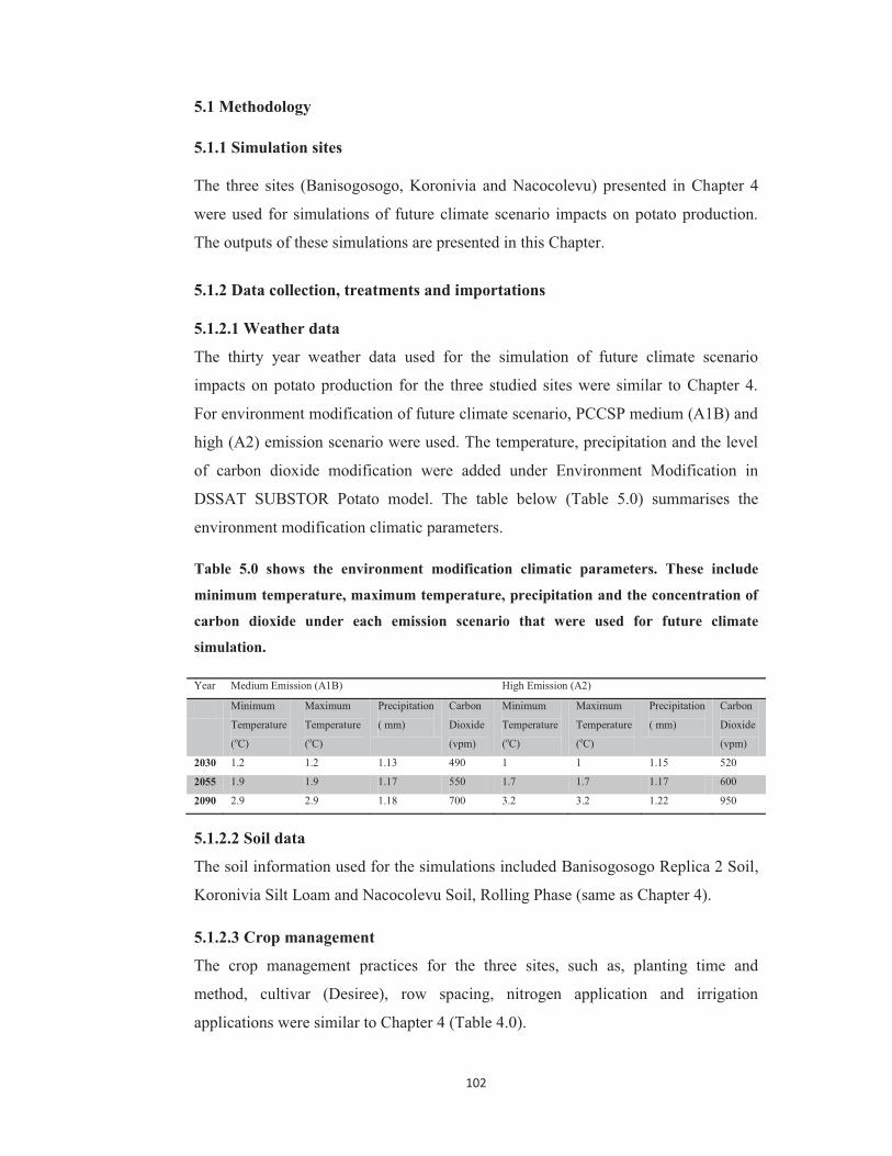
102
5.1 Methodology
5.1.1 Simulation sites
The three sites (Banisogosogo, Koronivia and Nacocolevu) presented in Chapter 4
were used for simulations of future climate scenario impacts on potato production.
The outputs of these simulations are presented in this Chapter.
5.1.2 Data collection, treatments and importations
5.1.2.1 Weather data
The thirty year weather data used for the simulation of future climate scenario
impacts on potato production for the three studied sites were similar to Chapter 4.
For environment modification of future climate scenario, PCCSP medium (A1B) and
high (A2) emission scenario were used. The temperature, precipitation and the level
of carbon dioxide modification were added under Environment Modification in
DSSAT SUBSTOR Potato model. The table below (Table 5.0) summarises the
environment modification climatic parameters.
Table 5.0 shows the environment modification climatic parameters. These include
minimum temperature, maximum temperature, precipitation and the concentration of
carbon dioxide under each emission scenario that were used for future climate
simulation.
Year Medium Emission (A1B) High Emission (A2)
Minimum
Temperature
(oC)
Maximum
Temperature
(oC)
Precipitation
( mm)
Carbon
Dioxide
(vpm)
Minimum
Temperature
(oC)
Maximum
Temperature
(oC)
Precipitation
( mm)
Carbon
Dioxide
(vpm)
2030 1.2 1.2 1.13 490 1 1 1.15 520
2055 1.9 1.9 1.17 550 1.7 1.7 1.17 600
2090 2.9 2.9 1.18 700 3.2 3.2 1.22 950
5.1.2.2 Soil data
The soil information used for the simulations included Banisogosogo Replica 2 Soil,
Koronivia Silt Loam and Nacocolevu Soil, Rolling Phase (same as Chapter 4).
5.1.2.3 Crop management
The crop management practices for the three sites, such as, planting time and
method, cultivar (Desiree), row spacing, nitrogen application and irrigation
applications were similar to Chapter 4 (Table 4.0).
103
5.1.3 Optimisation treatments
The simulation for optimisation of crop managements (planting date, row spacing,
planting depth and irrigation and fertiliser amount) to maximise Desiree growth and
yield was conducted using Sensitivity Analysis Option in the DSSAT SUBSTOR
Potato model with available weather and soil data. Weather data of 2012 was used to
conduct Banisogosogo optimisation treatments (except for planting time). The
Koronivia and Nacocolevu optimisation was conducted with 2010 weather data. The
planting time for all three sites was conducted with 2009 weather data. The
optimisation treatments and default runs were similar to optimisation treatments in
Chapter 4.
5.1.4 Model output analysis
The above inputs (soil data, weather data and crop management data) were used to
run the simulations for future climate impacts on potato growth and yield. All
summary outputs, graphical and initial analysis were done in DSSAT 4.5 Output.
Other statistical analysis was conducted in Microsoft 2007 Excel Spreadsheet. These
outputs are presented in the results section.
5.2 Results
The impacts of future climatic scenario were simulated on potato production in Fiji
using calibrated DSSAT SUBSTOR Potato model. In this study, two PSSCP climate
scenarios were used. The emission scenario included medium emission scenario
(A1B) and high emission scenario (A2) for three time periods (2030, 2055 and
2090). The weather data of Banisogosogo, Koronivia and Nacocolevu were modified
under the Environment Modification in DSSAT SUBSTOR Potato model. These
modification included changes in minimum temperature, maximum temperature,
precipitation and the concentration of carbon dioxide under each emission scenario
as stated by PSSCP Country Reports (Fiji). The results are divided into two sections;
(i) the future climate simulations with potential and non-potential production and (ii)
the optimisation treatments.
The future climate simulation, for the three locations, indicated that the number of
days for tuber initiation increased while the tuber fresh and dry weight decreased.
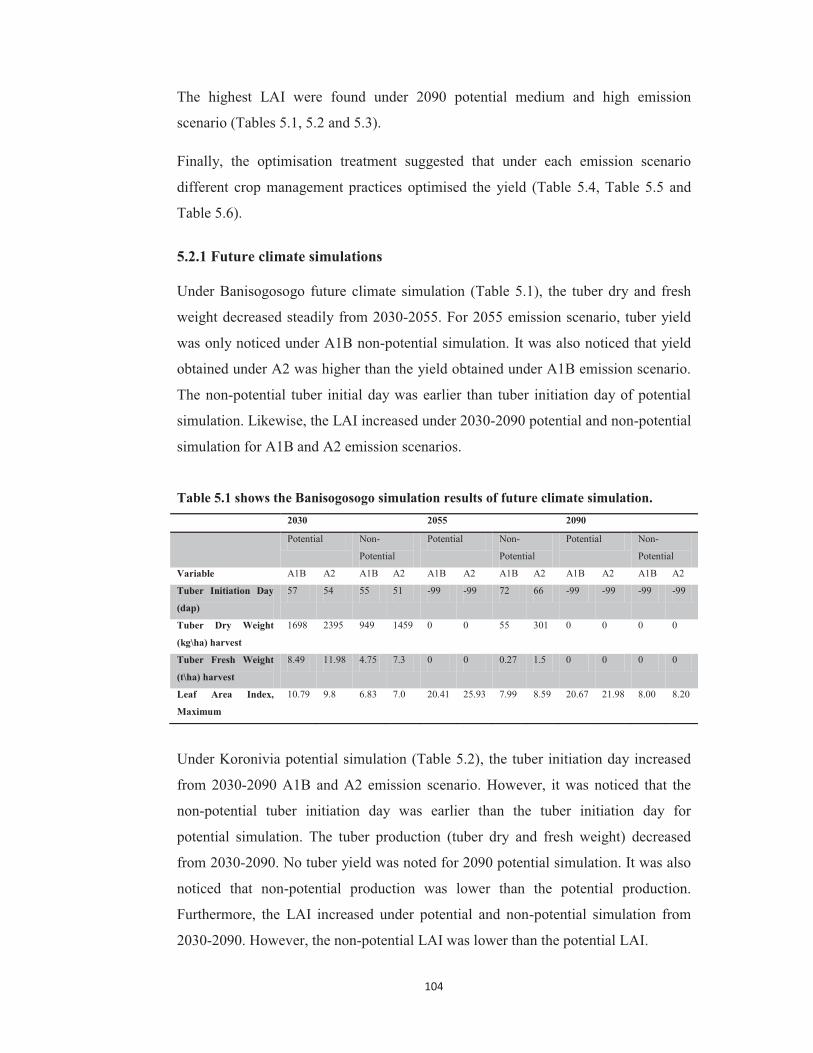
104
The highest LAI were found under 2090 potential medium and high emission
scenario (Tables 5.1, 5.2 and 5.3).
Finally, the optimisation treatment suggested that under each emission scenario
different crop management practices optimised the yield (Table 5.4, Table 5.5 and
Table 5.6).
5.2.1 Future climate simulations
Under Banisogosogo future climate simulation (Table 5.1), the tuber dry and fresh
weight decreased steadily from 2030-2055. For 2055 emission scenario, tuber yield
was only noticed under A1B non-potential simulation. It was also noticed that yield
obtained under A2 was higher than the yield obtained under A1B emission scenario.
The non-potential tuber initial day was earlier than tuber initiation day of potential
simulation. Likewise, the LAI increased under 2030-2090 potential and non-potential
simulation for A1B and A2 emission scenarios.
Table 5.1 shows the Banisogosogo simulation results of future climate simulation. 2030 2055 2090
Potential Non-
Potential
Potential Non-
Potential
Potential Non-
Potential
Variable A1B A2 A1B A2 A1B A2 A1B A2 A1B A2 A1B A2
Tuber Initiation Day
(dap)
57 54 55 51 -99 -99 72 66 -99 -99 -99 -99
Tuber Dry Weight
(kg\ha) harvest
1698 2395 949 1459 0 0 55 301 0 0 0 0
Tuber Fresh Weight
(t\ha) harvest
8.49 11.98 4.75 7.3 0 0 0.27 1.5 0 0 0 0
Leaf Area Index,
Maximum
10.79 9.8 6.83 7.0 20.41 25.93 7.99 8.59 20.67 21.98 8.00 8.20
Under Koronivia potential simulation (Table 5.2), the tuber initiation day increased
from 2030-2090 A1B and A2 emission scenario. However, it was noticed that the
non-potential tuber initiation day was earlier than the tuber initiation day for
potential simulation. The tuber production (tuber dry and fresh weight) decreased
from 2030-2090. No tuber yield was noted for 2090 potential simulation. It was also
noticed that non-potential production was lower than the potential production.
Furthermore, the LAI increased under potential and non-potential simulation from
2030-2090. However, the non-potential LAI was lower than the potential LAI.

105
Table 5.2 shows the Koronivia simulation results of future climate simulation. 2030 2055 2090
Potential Non-Potential Potential Non-
Potential
Potential Non-
Potential
Variable A1B A2 A1B A2 A1B A2 A1B A2 A1B A2 A1B A2
Tuber Initiation Day
(dap)
42 40 37 36 49 47 45 43 -99 -99 54 62
Tuber Dry Weight
(kg\ha) harvest
5909 6935 2369 2713 2615 4246 1578 2290 0 0 617 233
Tuber Fresh Weight
(t\ha) harvest
29.54 34.68 11.84 13.56 13.08 21.23 7.89 11.45 0 0 3.08 1.16
Leaf Area Index,
Maximum
12.68 11.99 4.03 3.98 16.83 20.14 4.7 4.81 35.41 38.41 6.04 6.92
For Nacocolevu simulations (Table 5.3), tuber yield was possible under 2030, 2055
and 2090 potential and non-potential simulation for A1B and A2 emission scenario.
Eventhough, production was possible under all emission scenario, a steady decrease
in tuber fresh and tuber dry weight was noted for both potential and non-potential
simulation. The results also suggest that non-potential production was lower than
potential production. The tuber initiation day also increased from 2030-2090
emission scenarios. It was also noted that the non-potential tuber initiation day were
earlier than potential simulation. Similarly, the LAI increased from 2030-2090 with
potential simulation showing higher value.
Table 5.3 shows Nacocolevu simulation results of future climate simulation.
2030 2055 2090
Potential Non-Potential Potential Non-
Potential
Potential Non-
Potential
Variable A1B A2 A1B A2 A1B A2 A1B A2 A1B A2 A1B A2
Tuber Initiation Day
(dap)
41 40 40 39 47 44 45 44 63 69 61 63
Tuber Dry Weight
(kg\ha) harvest
6584 7370 4908 5521 4093 6187 1993 2949 586 93 523 314
Tuber Fresh Weight
(t\ha) harvest
32.92 36.85 24.54 27.61 20.46 30.93 9.96 14.75 2.93 0.46 2.62 1.57
Leaf Area Index,
Maximum
6.87 6.64 3.55 3.19 7.81 8.34 5.00 4.69 12.07 15.64 5.68 5.74
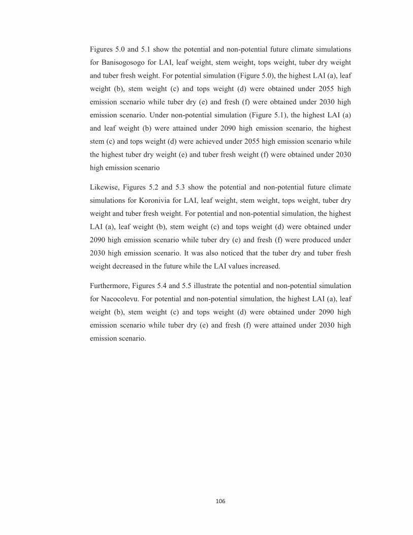
106
Figures 5.0 and 5.1 show the potential and non-potential future climate simulations
for Banisogosogo for LAI, leaf weight, stem weight, tops weight, tuber dry weight
and tuber fresh weight. For potential simulation (Figure 5.0), the highest LAI (a), leaf
weight (b), stem weight (c) and tops weight (d) were obtained under 2055 high
emission scenario while tuber dry (e) and fresh (f) were obtained under 2030 high
emission scenario. Under non-potential simulation (Figure 5.1), the highest LAI (a)
and leaf weight (b) were attained under 2090 high emission scenario, the highest
stem (c) and tops weight (d) were achieved under 2055 high emission scenario while
the highest tuber dry weight (e) and tuber fresh weight (f) were obtained under 2030
high emission scenario
Likewise, Figures 5.2 and 5.3 show the potential and non-potential future climate
simulations for Koronivia for LAI, leaf weight, stem weight, tops weight, tuber dry
weight and tuber fresh weight. For potential and non-potential simulation, the highest
LAI (a), leaf weight (b), stem weight (c) and tops weight (d) were obtained under
2090 high emission scenario while tuber dry (e) and fresh (f) were produced under
2030 high emission scenario. It was also noticed that the tuber dry and tuber fresh
weight decreased in the future while the LAI values increased.
Furthermore, Figures 5.4 and 5.5 illustrate the potential and non-potential simulation
for Nacocolevu. For potential and non-potential simulation, the highest LAI (a), leaf
weight (b), stem weight (c) and tops weight (d) were obtained under 2090 high
emission scenario while tuber dry (e) and fresh (f) were attained under 2030 high
emission scenario.
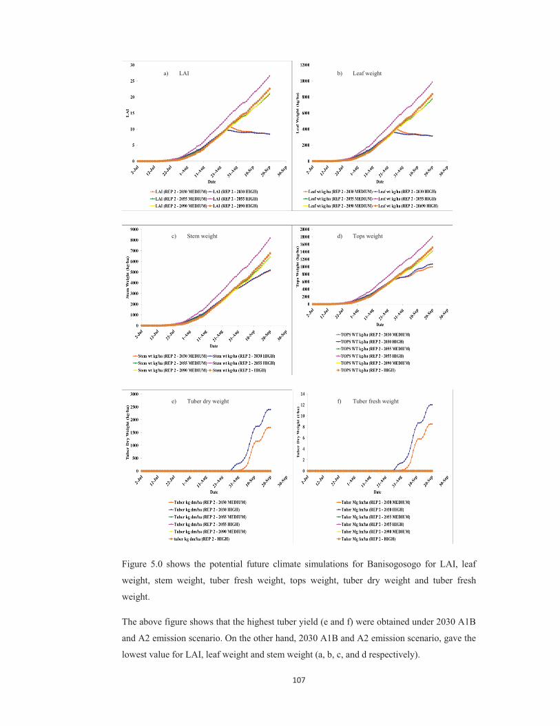
107
Figure 5.0 shows the potential future climate simulations for Banisogosogo for LAI, leaf
weight, stem weight, tuber fresh weight, tops weight, tuber dry weight and tuber fresh
weight.
The above figure shows that the highest tuber yield (e and f) were obtained under 2030 A1B
and A2 emission scenario. On the other hand, 2030 A1B and A2 emission scenario, gave the
lowest value for LAI, leaf weight and stem weight (a, b, c, and d respectively).
a) LAI b) Leaf weight
c) Stem weight
e) Tuber dry weight f) Tuber fresh weight
d) Tops weight

108
Figure 5.1 shows the non-potential future climate simulation for Banisogosogo under A1B
and A2 emission scenario for LAI, leaf weight, stem weight, tuber fresh weight, tuber dry
weight and tops weight.
The above figure illustrates that highest tuber weight (e and f) were achieved under 2030 A2,
followed by 2030 A1B, 2055 A2 and 2050 A1B emission scenario.
a) LAI
f) Tuber fresh weight
b) Leaf weight
c) Stem d) Tops weight
e) Tuber dry weight

109
Figure 5.2 shows the Koronivia potential future climate simulations for LAI, leaf weight,
stem weight, tuber fresh weight, tuber dry weight and tops weight.
The above figure shows that tuber yield (e and f) is possible under 2030-2055 A1B and A2
emission scenario while the highest LAI was recorded under 2090 A2 emission scenario.
a) LAI b) Leaf weight
c) Stem weight d) Tops weight
e) Tuber dry weight f) Tuber fresh weight

110
Figure 5.3 shows the Koronivia non-potential future climate simulations for LAI, leaf
weight, stem weight, tuber fresh weight, tuber dry weight and tops weight.
The above figure shows that under future climate, tuber yield is possible under 2030-2090
A1B and A2 emission scenario.
a) LAI b) Leaf weight
c) Stem weight d) Tops weight
e) Tuber dry weight f) Tuber fresh weight

111
Figure 5.4 shows the Nacocolevu potential future climate simulations for LAI, leaf weight,
stem weight, tuber fresh weight, tuber dry weight and tops weight.
The above figure shows that tuber yield is possible under 2030-2090 A1B and A2 emission
scenario.
a) LAI b) Leaf weight
c) Stem weight d) Tops weight
e) Tuber dry weight f) Tuber fresh weight

112
Figure 5.5 shows the Nacocolevu non-potential future climate simulation for LAI, leaf
weight, stem weight, tuber fresh weight, tuber dry weight and tops weight.
The figure above shows that under future climate, tuber yield is possible under 2030-2090
A1B and A2 emission scenario.
a) LAI b) Leaf weight
c) Stem weight d) Tops weight
e) Tuber dry weight f) Tuber fresh weight
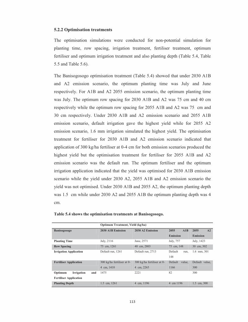
113
5.2.2 Optimisation treatments
The optimisation simulations were conducted for non-potential simulation for
planting time, row spacing, irrigation treatment, fertiliser treatment, optimum
fertiliser and optimum irrigation treatment and also planting depth (Table 5.4, Table
5.5 and Table 5.6).
The Banisogosogo optimisation treatment (Table 5.4) showed that under 2030 A1B
and A2 emission scenario, the optimum planting time was July and June
respectively. For A1B and A2 2055 emission scenario, the optimum planting time
was July. The optimum row spacing for 2030 A1B and A2 was 75 cm and 40 cm
respectively while the optimum row spacing for 2055 A1B and A2 was 75 cm and
30 cm respectively. Under 2030 A1B and A2 emission scenario and 2055 A1B
emission scenario, default irrigation gave the highest yield while for 2055 A2
emission scenario, 1.6 mm irrigation simulated the highest yield. The optimisation
treatment for fertiliser for 2030 A1B and A2 emission scenario indicated that
application of 300 kg/ha fertiliser at 0-4 cm for both emission scenarios produced the
highest yield but the optimisation treatment for fertiliser for 2055 A1B and A2
emission scenario was the default run. The optimum fertiliser and the optimum
irrigation application indicated that the yield was optimised for 2030 A1B emission
scenario while the yield under 2030 A2, 2055 A1B and A2 emission scenario the
yield was not optimised. Under 2030 A1B and 2055 A2, the optimum planting depth
was 1.5 cm while under 2030 A2 and 2055 A1B the optimum planting depth was 4
cm.
Table 5.4 shows the optimisation treatments at Banisogosogo.
Optimum Treatment, Yield (kg/ha)
Banisogosogo 2030 A1B Emission 2030 A2 Emission 2055 A1B
Emission
2055 A2
Emission
Planting Time July, 2116 June, 2571 July, 757 July, 1423
Row Spacing 75 cm, 1261 40 cm, 2803 75 cm, 148 30 cm, 302
Irrigation Application Default run, 1261 Default run, 2713 Default run,
148
1.6 mm, 301
Fertiliser Application 300 kg/ha fertiliser at 0-
4 cm, 1410
300 kg/ha fertiliser at 0-
4 cm, 2265
Default value,
1166
Default value,
300
Optimum Irrigation and
Fertiliser Application
1475 2221 82 300
Planting Depth 1.5 cm, 1261 4 cm, 1196 4 cm 1196 1.5 cm, 300
114
The Koronivia optimisation treatment (Table 5.5) showed that under 2030 and 2055
AIB and A2 emission scenario, the optimum planting time was August while under
2090 A1B and A2 emission scenario, the optimum planting time changed to July.
The optimum row spacing for 2030 A1B and A2 was 100 cm and 40 cm respectively
while 2055 A1B and A2 emission scenario, the optimum row spacing was 100 cm
and 80 cm respectively. A row spacing of 30 cm was required to produce the highest
yield under 2090 A1B and A2 emission scenario. Under 2030 A1B and A2 emission
scenario, 16.0 mm irrigation per plant gave the highest yield. Under 2055 A1B and
A2 emission scenario, 6.4 mm irrigation and default irrigation produced the highest
yield respectively whereas under 2090 A1B and A2 emission scenario, 1.6 mm per
plant irrigation attained the highest yield. The fertiliser optimisation treatment for
2030 A1B and A2 emission scenario indicated that application of 300 kg/ha fertiliser
at 0-4 cm for both emission scenarios simulated the highest yield. The optimisation
treatment for fertiliser for 2055 A1B and A2 emission scenario was application of 60
kg/ha fertiliser at 0-4 cm and default application of fertiliser respectively while
under 2090 A1B and A2 emission scenario, 60 kg/ha fertiliser produced the highest
yield. The optimum fertiliser and the optimum irrigation application indicated that
the yield was optimised for 2090 emission scenario. Under all emission scenarios,
the optimum planting depth was 1.5 cm.
Table 5.5 shows the optimisation treatments at Koronivia.
Optimum Treatment, Yield (kg/ha) Koronivia 2030 A1B
Emission 2030 A2 Emission
2055 A1B Emission
2055 A2 Emission
2090 A1B Emission
2090 A2 Emission
Planting Time August, 6692
August,7827 August, 3590
August, 5961
July, 1911 July, 1570
Row Spacing 100 cm, 2451
40 cm, 2803
100 cm, 1687
80 cm, 2331
30 cm, 667 30 cm, 291
Irrigation Application
16.0 mm, 3885
16.0 mm, 4911
6.4 mm, 2005
Default run, 2990
1.6 mm, 721
1.6 mm, 251
Fertiliser Application
300 kg/ha fertiliser at 0, 2, 4 cm, 2914
300 kg/ha fertiliser at 0, 2, 4 cm, 3400
60 kg/ha fertiliser at 0, 2, 4 cm, 2014
Default run, 2990
60 kg/ha fertiliser at 8 and 10 cm, 773
60 kg/ha fertiliser at 0-6 cm and 8 cm, 351
Optimum Irrigation and Fertiliser Application
3449 4342 1932 2100 779 401
Planting Depth 1.5 cm, 2369
1.5 cm, 2713
1.5 cm, 1578
1.5 cm, 300 1.5 cm, 617 1.5 cm, 233

115
The Nacocolevu optimisation treatment (Table 5.6) shows that under 2030 AIB and
A2 emission scenario, the optimum planting time was August while under 2055-
2090 A1B and A2 emission scenario, June was the optimum planting time. The
optimum row spacing for 2030 A1B and A2 was 75 cm and 100 cm respectively and
optimum row spacing for 2055 A1B and A2 was 100 cm and 40 cm respectively.
The optimum row spacing for 2090 A1B and A2 was 30 cm. Under 2030 A1B and
A2 emission scenario, 6.4 mm irrigation per plant and default irrigation simulated the
highest yield respectively. Under 2055 A1B and A2 emission scenario, 8.0 mm
irrigation and 16.0 mm irrigation gave the highest yield respectively. Under 2090
A1B and A2 emission scenario, 9.6 mm irrigation per plant and 16.0 mm irrigation
per plant produced the highest yield. The optimisation treatment for fertiliser for
2030 A1B and A2 emission scenario indicated that application of 300 kg/ha fertiliser
at 8 cm and default fertiliser application attained the highest yield respectively. The
optimisation treatment for fertiliser for 2055-2090 A1B and A2 emission scenario
was application of 60 kg/ha fertiliser. The optimum fertiliser and the optimum
irrigation application indicated that the yield was only optimised for 2030 A1B
emission scenario. Under 2030-2090 A1B and A2, the optimum planting depth was
1.5 cm.
Table 5.6 shows the optimisation treatments at Nacocolevu.
Optimum Treatment, Yield (kg/ha) Nacocolevu 2030 A1B
Emission 2030 A2 Emission
2055 A1B Emission
2055 A2 Emission
2090 A1B Emission
2090 A2 Emission
Planting Time August, 8178
August, 8522
June, 8141 June, 9385 June, 4729 June, 3634
Row Spacing 75 cm, 4908
100 cm, 6417
100 cm, 2182
40 cm, 3145
30 cm, 604 30 cm, 315
Irrigation Application
6.4 mm, 5125
Default run, 5521
8 mm, 2458 16 mm, 3131
9.6 mm, 680
16 mm, 320
Fertiliser Application
300 kg/ha fertiliser at 8 cm , 4997
Default run, 5611
60 kg/ha fertiliser at 6 cm, 3397
60 kg/ha fertiliser at 10 cm, 3946
60 kg/ha fertiliser at 0-4 cm, 1144
60 kg/ha fertiliser at 0-4 cm cm, 749
Optimum Irrigation and Fertiliser Application
5818 5549 3325 3808 974 612
Planting Depth 1.5 cm, 4908
1.5 cm, 5521
1.5 cm, 1993
1.5 cm, 2949
1.5 cm, 523 1.5 cm, 314

116
5.3 Discussion
5.3.1 Potential simulations
The Banisogosogo Desiree potential tuber yield was only possible under 2030
medium and 2030 high emission scenario. The Banisogosogo potential simulations
showed that under 2030 medium emission scenario the emergence day was 10th of
July (8 days after planting), tuber initiation day was 28th of August (57 days after
planting) with tuber dry yield of 1698 kg/ha, tuber fresh yield of 8.49 t/ha and LAI
was 10.79. Under 2030 high emission scenario, the emergence day was 10th of July,
tuber initiation day was 25th of August (54 days after planting) with tuber dry weight
of 2395 kg/ha, tuber fresh weight of 11.98 t/ha and LAI of 9.8. In other words, the
tuber initiation occurred three days earlier in 2030 high emission scenario compared
to 2030 medium emission scenario. This was because the projected temperature for
high emission scenario (1.2 oC) was less than the projected medium emission
scenario (1 oC). High temperatures caused an increase in abnormal tuber behavior,
chain tuber formation, secondary growth, growth cracks, heat sprouts, heat necrosis
and translucent ends. There is also reduction in starch, sucrose and dry matter content
of the tubers (Struik, 2007b). Above 30 oC, the net assimilation of potatoes fell below
zero and yield reduction occurs. There is reduction in partitioning of assimilation in
the tubers and improved partitioning at the haulm at high temperature (Levy and
Veilleux, 2007). It was also noted that the tuber initiation day and the maximum LAI
decreased from 2030 medium emission scenario to 2030 high emission scenario.
Under 2055 and 2090 medium and high emission scenario there was no tuber yield
but the LAI was higher under high emission scenario (Table 5.1). One reason for no
tuber yield can be due to the high average maximum and minimum temperatures
faced during the growing season which inhibited tuber initiation stage. As shown in
Figure 5.0, under 2030 medium and high emission scenario, the LAI and leaf weight
increased in weight from the planting date (2nd of July) until 25th of August. After
25th of August, the LAI and leaf weight started to decrease until the harvest date
while the tuber weight started to increase from 25th of August to the harvest date.
Under other emission scenarios (2055 and 2090 medium and high emission), there
was steady increase in LAI, leaf weight, stem weight and tops weight while there
was no tuber weight. Positive effects of elevated carbon dioxide has been observed
on potato yield (Schapendonk et al., 1995; Miglietta et al., 1998; Rosenzweig and

117
Hillel, 1998; Temmerman et al., 2000; Craigon et al., 2002; Te mmerman et al.,
2007; Hogy and Fangmeier, 2009a) but these increase in yields are highly species
dependent (Kimball, 1983). Tuber numbers also increased (P< 0.05) under elevated
carbon dioxide, particularly in the smaller size categories, that is, < 35 mm category
(Lawson et al., 2001b; K.Persson et al., 2003). The tuber quality also increased under
elevated carbon dioxide, that is, increase in the dry matter and starch concentration
(Donnelly et al., 2001; Vorne et al., 2002; Bucher and Kossmann, 2007; Te
mmerman et al., 2007), the concentrations of fructose, glucose and total reducing
carbohydrates were also positively related to carbon dioxide levels (Hogy and
Fangmeier, 2009b). One hypothesis that can be drawn from potatoes is that increased
sucrose availability under elevated carbon dioxide feeds forward to the production
and activity of the sink organs whereby resulting in increased yield (Te mmerman et
al., 2002). However, the concentration of nitrogen decreased (Fangmeier et al.,
2002). Doubling of carbon dioxide also caused earlier flowering, increased leaf area,
specific leaf weight, canopy density, plant height and accelerated crop maturation
rate (Krupa and Kickert, 1993). Conversely, elevated carbon dioxide had a negative
impact on tuber quality causing tuber malformation to increase by 62.8 % (Hogy and
Fangmeier, 2009b).
Under Koronivia potential simulations, 2030 medium emission scenario showed that
the emergence day was 9th of July (7 days after planting), tuber initiation day was
13th of August (42 days after planting) with tuber dry weight of 5909 kg/ha, tuber
fresh weight was 29.54 t/ha and LAI of 12.68. Under 2030 high emission scenario,
the emergence day was 9th of July, tuber initiation day was 11th of August (40 days
after planting) with tuber dry weight and fresh weight of 6935 kg/ha and 34.68 t/ha
and LAI of 11.99. The emission scenario of 2030 high emission showed a greater
yield as compared to 2030 medium emission scenario due to difference in
temperature increase and precipitation levels. It can also be said that for 2030 high
emission scenario, the tuber initiation day was earlier than 2030 medium emission
scenario. However, the LAI value was higher under 2030 medium emission scenario.
Under 2055 medium emission scenario it was shown that the emergence day was 10th
of July, tuber initiation day was 20th of August (49 days after planting) with tuber dry
weight and fresh weight of 2615 kg/ha and 13.08 t/ha and LAI of 16.83. The results
of 2055 high emission scenario indicated that the emergence day was 10th of July,

118
tuber initiation day was 18th of August (47 days after planting) with a tuber dry yield
of 4246 kg/ha, tuber fresh weight of 21.33 t/ha and LAI of 20.14. Under 2090
medium and high emission scenario, the emergence date was 12th of July and 13th of
July respectively. However, there were no tuber yield but the value of LAI was very
high (Table 5.2). This can be due to the high average maximum and minimum
temperatures experienced during the growing season which inhibited tuber initiation
development stage. Figure 5.2 indicated that under 2030 medium and high emission
scenario, the LAI, leaf weight and tops weight increased from the day of planting.
However, there was a decline in weight from 10th of August and 12th of August under
2030 medium and 2030 high emission scenario respectively. Under these emission
scenarios, tuber weight started to increase around the same time. For 2055 medium
and high emission scenario, the LAI, leaf weight and tops weight increased from the
day of planting until from 18th of August and 17th of August under 2030 medium and
2030 high emission scenario respectively. Under these emission scenarios, tuber
weight started to increase around the same time. Medium and high emission of 2090
showed gradual increase in LAI, leaf weight, stem weight and tops weight over time
with no tuber yield. Plants that are exposed to higher temperatures have smaller,
shorter, narrower and abundant leaves (Ewing and Struik, 1992). Warm temperatures
promotes vegetative growth while cool temperatures promotes tuber growth (Ewing,
1981c; Khedher and Ewing, 1985).
Nacocolevu produced yields in both medium and high emission scenarios from 2030
to 2090. The highest average temperature was experienced under 2090 medium and
high emission scenario which was 21.8 oC and 22.1 oC respectively. The optimum
temperature for potato production is 22 ºC (Burton, 1981). Table 5.3 indicated that
under 2030 medium emission scenario, the emergence day was 10th of July, tuber
initiation day was 12th of August (41 days after planting), the tuber dry weight was
6584 kg/ha, tuber fresh weight of 32.92 t/ha and LAI was 6.87. The results from
2030 high emission scenario indicated that the emergence day was 10th of July,
initiation of tuber was 11th of August (40 days after planting) with tuber dry weight
of 7370 kg/ha, tuber fresh weight was 36.85 t/ha and LAI of 6.64. The LAI also
decreased from 2030 medium emission to 2030 high emission. Under 2055 medium
emission scenario, the emergence day was 11th of July, tuber initiation day was 18th
of August (47 days after planting) with tuber dry weight and fresh weight was 4093

119
kg/ha and 20.46 t/ha and LAI of 7.81. The high emission of 2055 indicates that the
emergence day was 10th of July, tuber initiation day was 15th of August (44 days
after planting) with tuber dry weight of 6187 kg/ha, tuber fresh weight of 30.93 t/ha
with LAI of 8.34. The tuber dry yield decreased from year 2030 to 2055. The LAI
increased from the emission scenario of 2030 to 2055. Similar results are seen as LAI
increased from 2055 medium emission to 2055 high emission scenario. Finally, the
simulation for 2090 medium scenario indicated that the emergence day was 12th of
July, 3rd of September (63 days after planting) was noted for tuber initiation day.
Under this emission scenario, the tuber dry yield was 586 kg/ha with tuber fresh
weight of 2.93 t/ha and LAI of 12.07. Under 2090 high emission scenario it was seen
that the emergence day was 13th of July, tuber initiation day was 9th of September (63
days after planting) with tuber dry weight of 93 kg/ha, tuber fresh weight of 0.46 t/ha
and LAI of 15.64. Figure 5.4 showed that under 2030 and 2055 medium and high
emission scenario, the LAI, leaf weight, stem weight and tops weight increased from
the day of planting until 31st of August where a decline in weight was noticed. While
the tuber fresh weight started to increase from the 11th of August, 13th of August, 16th
of August, 19th of August and 4th of September for 2030 high, 2030 medium, 2055
high, 2055 medium and 2090 medium emission scenario respectively.
5.3.2 Non-potential simulations
Unlike Banisogosogo Desiree potential simulation which gave tuber yield only under
2030 emission scenario, Banisogosogo Desiree non-potential simulation showed that
tuber yield was sustained under 2030 medium and high emission scenario and 2055
medium and high emission scenario. The growth, development and yield of potatoes
are guided by factors such as high soil and high air temperature, plant density, water
stress, availability of nutrients and the utilisation of solar radiation (Allen, 1978;
Ewing, 1981b). The results from 2030 medium emission indicated that the
emergence day was 11th of July (9 days after planting), tuber initiation day was 26th
of August (55 days after planting) (Table 5.1). The tuber dry weight was 949 kg/ha,
tuber fresh weight of 4.75 t/ha and LAI of 6.83. The non-potential simulation shows
that the crop underwent water stress on 20th September (80 days after planting) and
nitrogen stress on 26th August (55 days after planting) and 20th September (refer to
Appendix 3.A for crop and soil status and environmental and stress factors for
Banisogosogo, Koronivia and Nacocolevu). Under 2030 high emission scenario, the
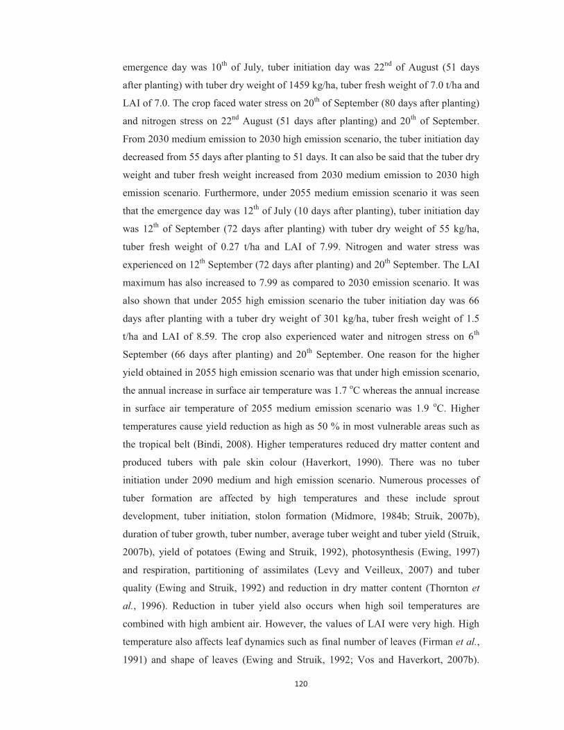
120
emergence day was 10th of July, tuber initiation day was 22nd of August (51 days
after planting) with tuber dry weight of 1459 kg/ha, tuber fresh weight of 7.0 t/ha and
LAI of 7.0. The crop faced water stress on 20th of September (80 days after planting)
and nitrogen stress on 22nd August (51 days after planting) and 20th of September.
From 2030 medium emission to 2030 high emission scenario, the tuber initiation day
decreased from 55 days after planting to 51 days. It can also be said that the tuber dry
weight and tuber fresh weight increased from 2030 medium emission to 2030 high
emission scenario. Furthermore, under 2055 medium emission scenario it was seen
that the emergence day was 12th of July (10 days after planting), tuber initiation day
was 12th of September (72 days after planting) with tuber dry weight of 55 kg/ha,
tuber fresh weight of 0.27 t/ha and LAI of 7.99. Nitrogen and water stress was
experienced on 12th September (72 days after planting) and 20th September. The LAI
maximum has also increased to 7.99 as compared to 2030 emission scenario. It was
also shown that under 2055 high emission scenario the tuber initiation day was 66
days after planting with a tuber dry weight of 301 kg/ha, tuber fresh weight of 1.5
t/ha and LAI of 8.59. The crop also experienced water and nitrogen stress on 6th
September (66 days after planting) and 20th September. One reason for the higher
yield obtained in 2055 high emission scenario was that under high emission scenario,
the annual increase in surface air temperature was 1.7 oC whereas the annual increase
in surface air temperature of 2055 medium emission scenario was 1.9 oC. Higher
temperatures cause yield reduction as high as 50 % in most vulnerable areas such as
the tropical belt (Bindi, 2008). Higher temperatures reduced dry matter content and
produced tubers with pale skin colour (Haverkort, 1990). There was no tuber
initiation under 2090 medium and high emission scenario. Numerous processes of
tuber formation are affected by high temperatures and these include sprout
development, tuber initiation, stolon formation (Midmore, 1984b; Struik, 2007b),
duration of tuber growth, tuber number, average tuber weight and tuber yield (Struik,
2007b), yield of potatoes (Ewing and Struik, 1992), photosynthesis (Ewing, 1997)
and respiration, partitioning of assimilates (Levy and Veilleux, 2007) and tuber
quality (Ewing and Struik, 1992) and reduction in dry matter content (Thornton et
al., 1996). Reduction in tuber yield also occurs when high soil temperatures are
combined with high ambient air. However, the values of LAI were very high. High
temperature also affects leaf dynamics such as final number of leaves (Firman et al.,
1991) and shape of leaves (Ewing and Struik, 1992; Vos and Haverkort, 2007b).
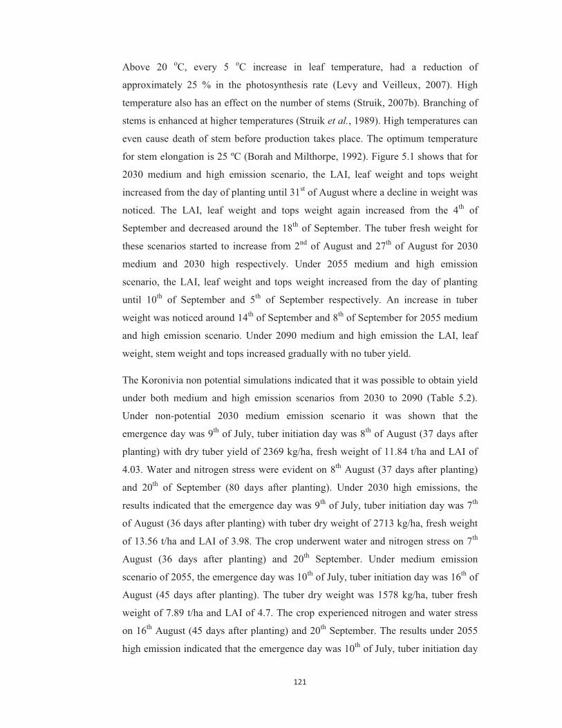
121
Above 20 oC, every 5 oC increase in leaf temperature, had a reduction of
approximately 25 % in the photosynthesis rate (Levy and Veilleux, 2007). High
temperature also has an effect on the number of stems (Struik, 2007b). Branching of
stems is enhanced at higher temperatures (Struik et al., 1989). High temperatures can
even cause death of stem before production takes place. The optimum temperature
for stem elongation is 25 ºC (Borah and Milthorpe, 1992). Figure 5.1 shows that for
2030 medium and high emission scenario, the LAI, leaf weight and tops weight
increased from the day of planting until 31st of August where a decline in weight was
noticed. The LAI, leaf weight and tops weight again increased from the 4th of
September and decreased around the 18th of September. The tuber fresh weight for
these scenarios started to increase from 2nd of August and 27th of August for 2030
medium and 2030 high respectively. Under 2055 medium and high emission
scenario, the LAI, leaf weight and tops weight increased from the day of planting
until 10th of September and 5th of September respectively. An increase in tuber
weight was noticed around 14th of September and 8th of September for 2055 medium
and high emission scenario. Under 2090 medium and high emission the LAI, leaf
weight, stem weight and tops increased gradually with no tuber yield.
The Koronivia non potential simulations indicated that it was possible to obtain yield
under both medium and high emission scenarios from 2030 to 2090 (Table 5.2).
Under non-potential 2030 medium emission scenario it was shown that the
emergence day was 9th of July, tuber initiation day was 8th of August (37 days after
planting) with dry tuber yield of 2369 kg/ha, fresh weight of 11.84 t/ha and LAI of
4.03. Water and nitrogen stress were evident on 8th August (37 days after planting)
and 20th of September (80 days after planting). Under 2030 high emissions, the
results indicated that the emergence day was 9th of July, tuber initiation day was 7th
of August (36 days after planting) with tuber dry weight of 2713 kg/ha, fresh weight
of 13.56 t/ha and LAI of 3.98. The crop underwent water and nitrogen stress on 7th
August (36 days after planting) and 20th September. Under medium emission
scenario of 2055, the emergence day was 10th of July, tuber initiation day was 16th of
August (45 days after planting). The tuber dry weight was 1578 kg/ha, tuber fresh
weight of 7.89 t/ha and LAI of 4.7. The crop experienced nitrogen and water stress
on 16th August (45 days after planting) and 20th September. The results under 2055
high emission indicated that the emergence day was 10th of July, tuber initiation day

122
was 14th of August (43 days after planting) with tuber dry weight was 2290 kg/ha,
tuber dry weight of 11.45 t/ha and LAI of 4.81. The crop faced nitrogen and water
stress on 14th August (43 days after planting) and 20th September. Furthermore,
under medium emission of 2090 it was noted that the emergence day was 12th of
July, tuber initiation day was 25th of August (54 days after planting) with tuber dry
weight of 617 kg/ha, tuber fresh weight of 3.08 t/ha and LAI of 6.04. The crop
suffered nitrogen and water stress on 25th August (85 days after planting) and 20th
September. Under 2090 high emission scenario, the emergence day was 13th of July,
tuber initiation day was 2nd of September (62 days after planting). The simulated
tuber dry weight was 233 kg/ha with tuber fresh weight of 1.16 t/ha and LAI of 6.92.
Water and nitrogen stress were seen on 2nd September (62 days after planting) and
20th September. Figure 5.3 shows that LAI, leaf weight and stem weight were the
highest under 2090 medium emission scenario and lowest under 2030 high emission
scenario. The final dry matter concentration depends on the cultivar, length of
growing seasons, water availability, solar intensity and the average temperature
during the growing season (Haverkort and Verhagen, 2008). Figure 5.3 showed that
the LAI, stem weight, leaf weight and tops weight increased from the day of planting
until around 9th of August. After 9th of August it experienced a decline in weight 28th
of August, after which it again increased in weight around 5th of September and then
decreased in weight around 5th of September. The figure also showed that the tuber
weight increased from 22nd of August and after 28th of August there was a sharp
increase in tuber weight until harvest. Overall, the tuber fresh and tuber dry weight
was highest under 2030 high emission scenario, followed by 2030 medium emission
scenario, 2055 high emission, 2055 medium emission, 2090 medium emission and
the lowest under 2090 high emission scenario. High temperatures significantly affect
potato growth and development (Food and Agriculture Organization of the United
Nations, 2008). Projections from simulation models indicate that higher temperatures
will reduce agronomic outputs. Farmers need to be mindful of local climate and their
ability to mitigate and adapt to these changing conditions (Mendelsohn and Dinar,
1999). Another significant finding from this study was that under potential
simulations production of potatoes is only possible from 2030-2055 under both
medium and high emission scenario while under non-potential simulation,
production of potato was possible from 2030 to 2090 under both medium and high
emission scenario. It can be said that the tuber initiation day was the earliest under

123
2030 high emission followed by 2030 medium emission, 2055 high emission, 2055
medium emission, 2090 medium emission and finally 2090 high emission. It was
also noticed that LAI increased from 2030-2090. Under elevated carbon dioxide
there is an increase in leaf number due to shift in temporal crop development
(Lawson et al., 2001c).
Nacocolevu non potential simulations show that it was possible to obtain yield under
both medium and high emission scenarios from 2030 to 2090 (Table 5.3). One reason
for this can be that there was no evidence of water stress in Nacocolevu during the
potato growing season. Under non-potential 2030 medium emission scenario it was
shown that emergence day was 10th of July, tuber initiation day was 11th of August
(40 days after planting) with dry tuber yield of 4908 kg/ha, fresh weight of 24.54 t/ha
and LAI of 3.55. Nitrogen stress was evident on 11th August (40 days after planting)
and 20th of September (80 days after planting). Under 2030 high emissions, the
results indicated that the emergence day was 10th of July, tuber initiation day was
10th of August (39 days after planting) with tuber dry weight of 5521 kg/ha, tuber
fresh weight of 27.61 t/ha and LAI of 3.19. The crop underwent nitrogen stress on
10th August (39 days after planting) and 20th September. Under medium emission
scenario of 2055, the emergence day was 11th of July, tuber initiation day was 16th of
August (45 days after planting). The tuber dry weight was 1993 kg/ha, tuber fresh
weight of 9.96 t/ha and LAI of 5.0. The plant underwent nitrogen stress under 16th
August (45 days after planting) and 20th September. For 2055 high emission it was
seen that the emergence day was 11th of July, tuber initiation day was 15th of August
(44 days after planting). The tuber dry weight was 2949 kg/ha, tuber fresh weight of
14.75 t/ha and LAI of 4.69. Nitrogen stress was evident on the plant on 15th of
August (44 days after planting) and 20th of September. Under medium emission of
2090, it was noted that the emergence day was 13th of July, the tuber initiation day
was 1st of September (61 days after planting) with tuber dry weight of 523 kg/ha and
tuber fresh weight of 2.62 t/ha and LAI of 5.68. Nitrogen stress was seen on 1st
September (61 days after planting) and 20th September. Under 2090 high emission
scenario the emergence day was 13th of July, tuber initiation day was 3rd of
September (63 days after planting). The simulated tuber dry weight was 314 kg/ha,
tuber fresh weight of 314 t/ha and LAI of 5.74. Nitrogen stress was seen on 3rd of
September (63 days after planting) and 20th September. Figure 5.5 indicated that the
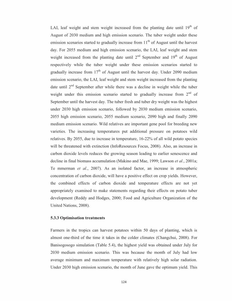
124
LAI, leaf weight and stem weight increased from the planting date until 19th of
August of 2030 medium and high emission scenario. The tuber weight under these
emission scenarios started to gradually increase from 11th of August until the harvest
day. For 2055 medium and high emission scenario, the LAI, leaf weight and stem
weight increased from the planting date until 2nd September and 19th of August
respectively while the tuber weight under these emission scenarios started to
gradually increase from 17th of August until the harvest day. Under 2090 medium
emission scenario, the LAI, leaf weight and stem weight increased from the planting
date until 2nd September after while there was a decline in weight while the tuber
weight under this emission scenario started to gradually increase from 2nd of
September until the harvest day. The tuber fresh and tuber dry weight was the highest
under 2030 high emission scenario, followed by 2030 medium emission scenario,
2055 high emission scenario, 2055 medium scenario, 2090 high and finally 2090
medium emission scenario. Wild relatives are important gene pool for breeding new
varieties. The increasing temperatures put additional pressure on potatoes wild
relatives. By 2055, due to increase in temperature, 16-22% of all wild potato species
will be threatened with extinction (InfoResources Focus, 2008). Also, an increase in
carbon dioxide levels reduces the growing season leading to earlier senescence and
decline in final biomass accumulation (Makino and Mae, 1999; Lawson et al., 2001a;
Te mmerman et al., 2007). As an isolated factor, an increase in atmospheric
concentration of carbon dioxide, will have a positive effect on crop yields. However,
the combined effects of carbon dioxide and temperature effects are not yet
appropriately examined to make statements regarding their effects on potato tuber
development (Reddy and Hodges, 2000; Food and Agriculture Organization of the
United Nations, 2008).
5.3.3 Optimisation treatments
Farmers in the tropics can harvest potatoes within 50 days of planting, which is
almost one-third of the time it takes in the colder climates (Changchui, 2008). For
Banisogosogo simulation (Table 5.4), the highest yield was obtained under July for
2030 medium emission scenario. This was because the month of July had low
average minimum and maximum temperature with relatively high solar radiation.
Under 2030 high emission scenario, the month of June gave the optimum yield. This
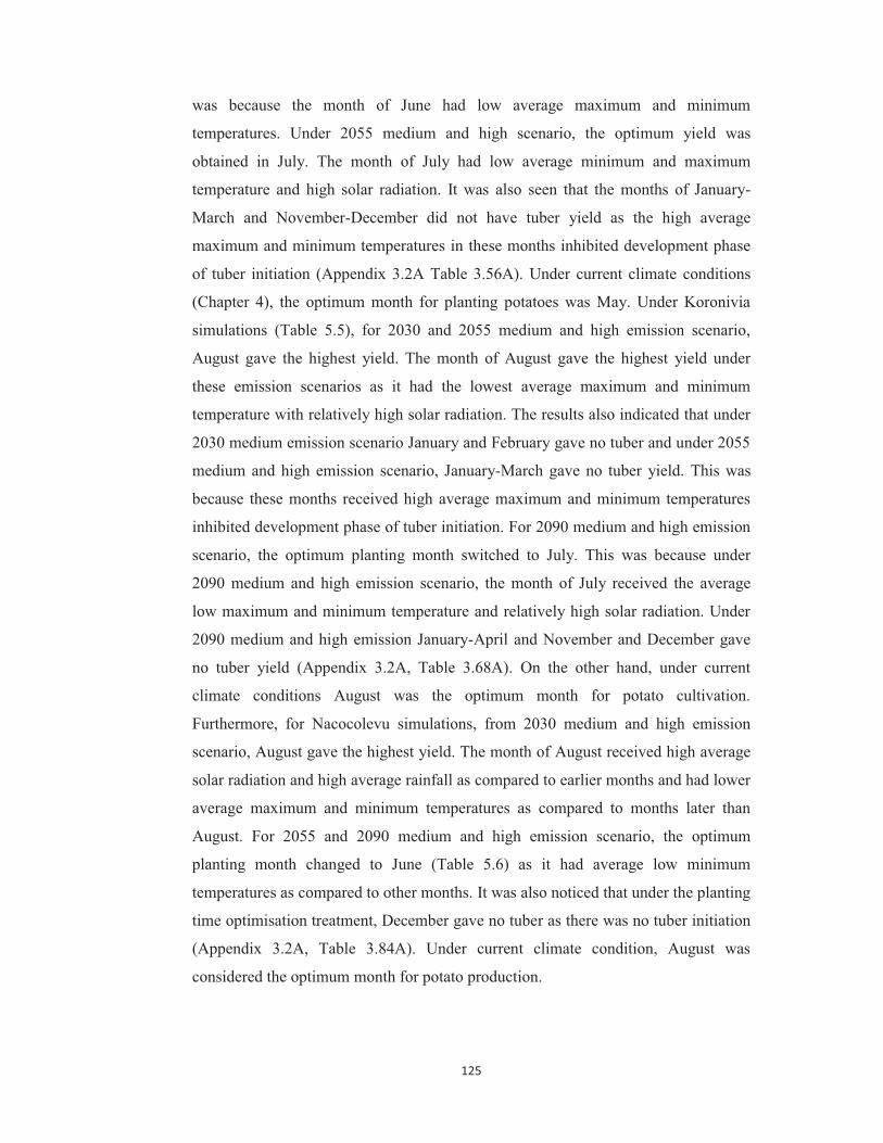
125
was because the month of June had low average maximum and minimum
temperatures. Under 2055 medium and high scenario, the optimum yield was
obtained in July. The month of July had low average minimum and maximum
temperature and high solar radiation. It was also seen that the months of January-
March and November-December did not have tuber yield as the high average
maximum and minimum temperatures in these months inhibited development phase
of tuber initiation (Appendix 3.2A Table 3.56A). Under current climate conditions
(Chapter 4), the optimum month for planting potatoes was May. Under Koronivia
simulations (Table 5.5), for 2030 and 2055 medium and high emission scenario,
August gave the highest yield. The month of August gave the highest yield under
these emission scenarios as it had the lowest average maximum and minimum
temperature with relatively high solar radiation. The results also indicated that under
2030 medium emission scenario January and February gave no tuber and under 2055
medium and high emission scenario, January-March gave no tuber yield. This was
because these months received high average maximum and minimum temperatures
inhibited development phase of tuber initiation. For 2090 medium and high emission
scenario, the optimum planting month switched to July. This was because under
2090 medium and high emission scenario, the month of July received the average
low maximum and minimum temperature and relatively high solar radiation. Under
2090 medium and high emission January-April and November and December gave
no tuber yield (Appendix 3.2A, Table 3.68A). On the other hand, under current
climate conditions August was the optimum month for potato cultivation.
Furthermore, for Nacocolevu simulations, from 2030 medium and high emission
scenario, August gave the highest yield. The month of August received high average
solar radiation and high average rainfall as compared to earlier months and had lower
average maximum and minimum temperatures as compared to months later than
August. For 2055 and 2090 medium and high emission scenario, the optimum
planting month changed to June (Table 5.6) as it had average low minimum
temperatures as compared to other months. It was also noticed that under the planting
time optimisation treatment, December gave no tuber as there was no tuber initiation
(Appendix 3.2A, Table 3.84A). Under current climate condition, August was
considered the optimum month for potato production.

126
Row spacing also had an impact on tuber yield. As indicated in Table 5.4
Banisogosogo 2030 medium emission scenario results of row spacing indicated that
to maximise potato yield, a row spacing of 75 cm was suitable. The results 2030 high
emission scenario of row spacing indicated that a row spacing of 40 cm produced
the highest yield of 2803 kg/ha. Under 2055 medium and high emission scenario, it
was noted that a row spacing of 75 cm and 30 cm gave the highest yield respectively
(Appendix 3A, Table 3.57). Table 5.5 shows that under Koronivia 2030 medium
emission scenario, the simulation of row spacing indicated that maximum yield can
be achieved at a row spacing of 100 cm which simulated a yield of 2451 kg/ha.
Under 2030 high emission scenario, row spacing of 40 cm gave the highest tuber
yield. For 2055 medium emission scenario, row spacing of 100 cm produced the
highest yield. The results of 2055 high emission scenario indicated that a row
spacing of 80 cm produced the highest yield at 2331 kg/ha. For 2090 medium and
high emission scenario, row spacing of 30 cm gave the highest yield (Appendix 3A,
Table 3.69). For Nacocolevu 2030 medium emission scenario, the simulation of row
spacing indicated that maximum yield can be achieved at a row spacing of 75 cm
which gave a yield of 4908 kg/ha. Under 2030 medium emission, the simulation of
row spacing has shown that increasing the row spacing increased the tuber yield.
Hence, at row spacing of 100 cm, the highest yield tuber yield was obtained at 6417
kg/ha. For Nacocolevu 2055 medium emission scenario a row spacing of 100 cm
gave the highest yield. For Nacocolevu 2055 high emission scenario simulation, the
results of row spacing indicated that a row spacing of 40 cm gave the highest yield at
3145 kg/ha. For Nacocolevu 2090 medium emission scenario simulation, the results
of row spacing indicated that row spacing of 30 cm gave the highest yield under
2090 medium emission. Increasing the row spacing decreased the tuber yield. Under
2090 high emission scenario, the row spacing indicated that under 30 cm and 50 cm
of row spacing gave the highest yield (315 kg/ha). The lowest yield was achieved
under 100 cm (Table 5.6 and Appendix 3A, Table 3.85).
Likewise, optimisation simulation was also conducted for fertiliser treatment. The
results for Banisogosogo 2030 medium and high emission scenario fertiliser
treatment indicated that application of 300 kg/ha fertiliser at 0-4 cm simulated the
highest yield (1410 kg/ha and 2265 respectively). Under 2055 medium emission
results for fertiliser treatment indicated that default run gave the highest yield at 148

127
kg/ha while under 2055 high emission scenario, 60 kg/ha at 0-4 cm gave the highest
yield at 304 kg/ha (Appendix 3.2A, Tables 3.60A, 3.62A, 3.64A and 3.66A). For
Koronivia simulations, under 2030 medium and high emission scenario and 2055
medium emission scenario, fertiliser optimisation results indicated that application of
300 kg/ha fertiliser at depth of 0 cm, 2 cm and 4 cm gave maximum yield. For 2055
high emission scenario, default run produced the highest yield at 2990 kg/ha. For
2090 medium emission scenario, application of 60 kg/ha fertiliser at 8 and 10 cm
simulated the highest yield at 773 kg/ha while under 2090 high emission scenario
fertiliser optimisation treatment indicated that maximum yield of tuber can be
obtained under 60 kg/ha of fertiliser treatment at 0-6 cm and 8 cm (Appendix 3.2A,
Tables 3.72A, 3.74A, 3.76A, 3.78A, 3.80A and 3.82A). For Nacocolevu 2030
medium, the fertiliser optimisation results indicated that application of 300 kg/ha
fertiliser at depth of 8 cm gave maximum yield of 4997 kg/ha. Under 2030 high
emission, the default run gave the highest yield. For Nacocolevu 2055 medium
emission scenario simulation, the optimum fertiliser treatment indicated that
application of 60 kg/ha of fertiliser at 6 cm gave maximum yield at 3397 kg/ha.
Under Nacocolevu 2055 high emission scenario simulation, the results of fertiliser
treatment indicated that application of 60 kg/ha fertiliser at 10 cm simulated the
highest yield at 3946 kg/ha. Finally Nacocolevu 2090 and high medium emission
scenario simulation, the fertiliser optimisation treatment indicated that maximum
yield of tuber can be obtained under 60 kg/ha of fertiliser treatment at 0 cm, 2 cm
and 4 cm with tuber yield of 1144 kg/ha and 749 kg/ha respectively (Table 5.6,
Appendix 3.2A, Tables 3.88A, 3.90A, 3.92A, 3.94A, 3.96A and 3.98A).
Furthermore, optimisation was also conducted for irrigation application. Table 5.5
indicates that for Banisogosogo irrigation optimisation, under 2030 medium and high
emission scenario and 2055 medium emission scenario, the default run gave the
highest yield while under 2055 high emission scenario, 1.6 mm of irrigation per plant
gave the highest yield at 301 kg/ha (also refer to Appendix 3.2A, Table 3.58A).
Under 2030 medium and 2030 high emission scenario for Koronivia, the results of
the irrigation optimisation in general suggested that an increase in irrigation levels
increased yield. Hence, the highest yield was obtained at 16 mm and the lowest yield
was obtained at 1.6 mm. Under 2055 medium emission scenario, the results indicated
that application of irrigation of 6.4 mm per plant produced the highest yield at 2005

128
kg/ha. The lowest yield was recorded at 1.6 mm irrigation with tuber yield at 1874
kg/ha. Under 2055 high emission scenario, the results from irrigation simulation
indicated that the highest yield was obtained under default run at 721 kg/ha. For 2090
medium and high emission scenario, the irrigation treatment indicated that increasing
the amount of irrigation decreased the tuber yield hence the highest yield was
obtained under irrigation application of 1.6 mm (Table 5.5 and also refer to
Appendix 3A, Table 3.70A). For all emission scenario at Nacocolevu, under 2030
medium emission scenario, 6.4 mm of irrigation gave the highest yield at 5125 kg/ha
while under 2030 high emission scenario the default run gave the highest yield.
Under 2055 medium emission scenario, application of 8 mm irrigation per plant gave
the highest yield at 2458 kg/ha while under 2055 high emission scenario, application
of 16.0 mm gave the highest yield ay 3131 kg/ha. For 2090 medium and high
emission scenario, application of 9.6 mm and 16.0 mm gave the highest yield
respectively.
In addition to these, optimisation treatment was also conducted for optimum
irrigation and optimum fertiliser simulations. It was noticed that under Banisogosogo
simulations, higher yields were only obtained under 2030 high emission scenario
(Table 5.5). For Koronivia simulations it was noticed that, only 2090 medium and
high emission scenario managed to optimise the tuber yield (Table 5.6). Under
Nacocolevu simulations, only 2030 medium and high emissions optimised the yield.
Finally, optimisation was conducted to investigate how planting depth affected tuber
yield. Banisogosogo 2030 medium emission scenario, planting depth of 1.5 m gave
the highest yield. It was also noted that increasing the planting depth decreased the
yield. Planting depth of 8 m and 10 cm failed to produce any yield. Under 2030 high
emission scenario, a depth of 4 cm simulated the highest yield of 1196 kg/ha.
Planting potatoes at a depth of 1.5 cm and 6 cm gave the same yield at 1166 kg/ha.
Planting of potatoes at a depth of 8 cm gave the lowest yield. Under 2055 medium
emission scenario, planting depth of 4 cm attained the highest yield of 1196 kg/ha.
Planting potatoes at a depth of 8 cm gave the lowest yield at 32 kg/ha. Under 2055
high emission scenario, the best depth to plant potatoes for maximum yield was at
1.5 cm which gave a yield of 300kg/ha. Increasing the planting depth decreased the
yield. The results also indicated that planting potatoes at 4 cm, 6 cm and 8 cm gave
no yield (also refer to Appendix 3A, Table 3.59A). For Koronivia and Nacocolevu

129
simulations it was noticed that under all emission scenarios, potato seeds should be
planted at 1.5 cm to achieve the highest yield. Increasing the depth of planting
decreased the yield of potatoes (also refer to Appendix 3A, Tables 3.71A and Table
3.87A).
5.4 Recommendations
Climate change will lead to changes in planting dates. It is recommended that
cultivation timing for Banisogosogo under 2030 medium emission scenario should
take place in July to obtain the highest yield while under 2030 high emission
scenario, the planting time should be June. Under 2055 medium and high emission
scenario the cultivation timing should be July. For Koronivia, it is recommended that
under 2030-2055 medium and high emission scenario, the planting time should be
August while under 2090 medium and high emission scenario, the planting time
should be July. The cultivation timing for Nacocolevu under 2030 medium and high
emission scenario should be August while under 2055-2090 medium and high
emission scenario, the planting time should be July. Planting time is projected to take
place earlier than anticipated as the thermal environment experienced by the crop
canopies would be more favourable (Singh et al., 2009; Knox et al., 2010). Changes
in the amount photoperiod due to changes in planting time has not been taken into
account (Hijmans, 2003a).
Irrigation levels also have to be adjusted with changes in the climate. In some
climatic conditions, such as, Banisogosogo required minimal irrigation such as that
of default irrigation and irrigation of 1.6 mm per plant. Koronivia 2030 medium and
high emission scenario required irrigation of 16.0 mm per plant while 2055 medium
and high emission scenario required 6.4 mm and default irrigation respectively.
Under 2090 medium and high emission scenario, 1.6 mm of irrigation per plant is
required. Nacocolevu 2030 medium and high emissions, required irrigation of 6.4
mm and default irrigation respectively. The emission scenarios of 2055 medium and
high required 8.0 mm and 16.0 mm of irrigation respectively. Under 2090 medium
and high emission scenario, irrigation application of 9.6 mm and 16.0 mm was
required respectively. If irrigation is not available in the future during the tuber
bulking phase, then the potato industry will not be viable and husbandry issue will
cease to be relevant (Holden and Brereton, 2006). Water management is also seen as

130
a key area that requires adaptation for climate change. A wide range of agricultural
water management practices and technologies are available to buffer the production
risks. Improving water efficiency requires an understanding of how plants balance
their water status in relation to evaporation demand under different soil conditions
(Stalham and Allison, 2011). Improved irrigation technology is one option to
improve water efficiency (Vos and Haverkort, 2007b). Other options include
effective use of rainfall, encouraging deeper rooting of crops, introducing drought
tolerant varieties and soil modifying soil structure to improve water retention (Knox
et al., 2010) and partial root zone drying (Shahnazari et al., 2008; Jovanovica et al.,
2010a). Partial root drying zone treatment resulted in the increase of nitrogen, starch
content and antioxidant activity in the potato tubers (Jovanovica et al., 2010b).
To maximise potato yield in future climatic scenario, fertiliser application levels and
application depth has to be adjusted to suit the change in climatic conditions. In some
climatic conditions, such as, Banisogosogo 2030 medium and high emission
scenario, high fertiliser levels are required while in other future climate scenario,
such as, Koronivia and Nacocolevu 2055-2090 medium and high emission, low
fertiliser levels are required. For potato, halving of nitrogen application rates could
be achieved only if irrigation water was used (Holden and Brereton, 2006).
Finally, it is also important to pay attention to planting depth under future climatic
scenario. In many cases, it was noted that either 1.5 cm or 2 cm were suitable for
planting potatoes. Increasing the planting depth (6 cm and 8 cm) gave no tuber yield.
5.5 Research limitations
One of the major challenges faced in this research was getting hold of the weather
data. Hence, different locations were run with different number of weather data, for
example, Banisogosogo simulation was conducted with weather data of 1960-2012,
Koronivia potential and non-potential simulations were run using weather data from
1961-2010 and Nacocolevu potential and non-potential simulations were conducted
using weather data from July 1972-2010. The different number of weather data used
in these simulations made it difficult to compare one site with another site. The
calibration of the DSSAT SUBSTOR Potato model was conducted only for
Banisogosogo. To obtain more accurate results, the model should have also been
vcalibrated for Koronivia and Nacocolevu.
131
Secondly, under all the simulations, it is assumed that the crop management practices
and the soil physical and chemical properties remained unchanged.
Also, it was noticed that the Plantgro.Output did not provide 2090 high emission
graphics. Hence, Excel was used to merge 2090 high emission scenario graphics into
all the graphs.
Finally, for future research, it is suggested that DSSAT v4.6 be used as it has a better
response to carbon dioxide concentration and better response to radiation use
efficiency.
132
Chapter 6 Simulating the performance of potential potato varieties under
current and future climates in Banisogosogo, Fiji Islands.
6.0 Introduction
There is a need to identify potato varieties in Fiji which may perform better under
current and future climatic conditions. Most of the countries in the Asia and Pacific
region are utilising potato varieties that were bred for growing conditions of Europe
or United States. These varieties are not adapted to the agroclimatic conditions of the
country where they are grown. Since many of these countries do not have suitable
research and development systems for native varieties, the cultivation of exotic
varieties cannot be stopped. However, these exotic varieties should be evaluated first
before they are recommended for large scale production (Singh, 2008).
Climate change poses a great challenge for breeders. To address these challenges,
development of new skills and qualification are required as potato breeding has
become more rooted in basic science and to be more receptive to public concerns
(Bonnel, 2008). Therefore, it is very important to monitor potato growth and forecast
its yield well before the harvest so that planners, decision makers and the
government can focus on its import and export and also redistribute food in times of
disasters. Forecasting the yields is also important in regions with climatic
uncertainties (Bala and Islam, 2008).
Climate change has created the need for adapting to several characteristics at once.
There is an urgent need to breed new potato varieties that are better adapted to
changing climatic conditions. The CIP is focusing on breeding short season potato
varieties for farmers to avoid adverse conditions such as hot, dry periods and heavy
rainfall. The CIP is evaluating the genetic resources of its collection of potatoes and
also of new varieties which are in process of being bred in regards to water and
temperature stress (InfoResources Focus, 2008). The adaptation of potato to a wide
range of environmental conditions is necessary to sustain variation and diversity in
potatoes (Bradshaw, 2007). If such adaptation measures are not taken, the potato
production, under the impact of climate change and global warming may decline by
3.16% in 2020 and 13.72% in 2050 (Singh et al., 2009).

133
This chapter will discuss what other varieties of potato can be cultivated in Fiji under
current climate and future climate conditions.
6.1 Methodology
6.1.1 Model simulation under current climate
6.1.1.1 Simulation site
The site for simulation for other varieties performance in Fiji was Banisogosogo,
Rakiraki (as in Chapters 3 and 4).
6.1.1.2 Data collection, treatments and importations
The weather data and soil data for the studied site used in these simulations was
similar as in Chapter 4. The crop management practices for planting time and
method, row spacing, nitrogen application and irrigation applications presented in
Chapter 4 were also used in these simulations. The baseline variety was Desiree
(Chapters 3, 4 and 5). The other cultivars used for these simulations are Sebago and
Russet Burbank (Genetic co-efficient in Table 6.0)
Table 6.0 shows the genetic co-efficient of Sebago and Russet Burbank.
Variety Name ECO
Number
G2
G3 G4 PD P2 TC
Desiree
tropics
IB0001 4000 25.0 0.2 0.9 0.4 18.0
Sebago IB0001 1500 22.5 0.20 0.90 0.10 19.0
Russet
Burbank
IB0001 2000 26.0 0.20 0.90 0.6 17.0
6.1.1.3 Reasons for cultivar selection
The cultivars selected for the simulation were Sebago and Russet Burbank. Sebago
variety was selected for this simulation because it has been planted in Fiji before and
the Ministry of Agriculture is thinking of reintroducing it in Fiji. Sebago variety is a
90 day crop which can yield up to 9 t/ha (Autar, 2009). Russet Burbank was selected
for this simulation as a possible recommendation for potato production. It is a late
maturity crop and requires 140 to 150 days season to produce maximum yields (The
Potato Association for America, 2009).
134
6.1.1.4 Optimisation treatments
The optimisation of crop managements, such as, planting date, row spacing, planting
depth and irrigation and fertiliser amount to maximise Sebago and Russet Burbank
growth and yield was conducted using Sensitivity Analysis Option in the DSSAT
SUBSTOR Potato model. The Banisogosogo optimisation simulations were
conducted with 2012 weather data except for planting time which was conducted
with 2009 weather data. The baseline variety is Desiree (Chapters 4 and 5).
6.1.2 Model simulation under future climatic conditions
6.1.2.1 Simulation site
The simulation site (Banisogosogo) presented in Chapter 4 was used for simulations
of future climate scenario impacts on potato production. The outputs of these
simulations are presented in the Results section of this Chapter.
6.1.2.2 Data collection, treatments and importations
The weather data for Banisogosogo and the PCCSP climate emission scenarios used
for the studied site in these simulations was the same as presented in Chapter 5. The
soil information for the studied site used in these simulations was the same as in
Replica 2 soil, Banisogosogo in Chapters 4 and 5. The crop management practices,
such as, planting time, nitrogen application and irrigation applications presented in
Chapter 4 were also used in these simulations.
6.1.2.3 Optimisation treatments
The simulation for optimisation of crop managements (planting date, row spacing,
planting depth, irrigation application and fertiliser amount) to maximise Sebago and
Russet Burbank growth and yield was conducted using Sensitivity Analysis Option
in the DSSAT SUBSTOR Potato model. The Banisogosogo optimisation was
simulated using the 2012 weather data except for planting time which was conducted
with 2009 weather data.
6.1.3 Model output analysis
The above inputs (soil data, weather data and crop management data) were used to
run the simulations for future climate impacts on potato growth and yield. All
summary outputs, graphical and initial analysis were done in DSSAT 4.5 Output.

135
Other statistical analysis was conducted in Microsoft 2007 Excel Spreadsheet. These
outputs are presented in the Results section.
6.2 Results
This section describes the simulation of Sebago and Russet Burbank potato variety
growth and yield under current climate conditions in Banisogosogo using the DSSAT
SUBSTOR Potato Model. The impact of climate variability, El Niño Southern
Oscillation (ENSO) state, was also studied on potato yield for the two potato
varieties. In addition to these, optimisation treatments were also conducted to
investigate which crop management practices, such as planting date, row spacing,
irrigation treatment, fertiliser treatment, optimum irrigation and optimum fertiliser
treatment and planting depth can optimise potato yield.
6.2.1 Current climate simulations
The current climate simulation was conducted for Banisogosogo for Sebago and
Russet Burbank varieties (Table 6.1). The weight for potential production was higher
as there was no water and nitrogen stress faced by the plant. Under non-potential
conditions, the plant faced water and nitrogen stress which reduced the above-ground
and below-ground biomass. The results show that Sebago variety had earlier tuber
initiation day and higher tuber dry weight and tuber fresh weight under potential
production while Desiree had higher tuber fresh weight and tuber dry weight under
non-potential conditions. Russet Burbank variety had higher LAI.
Table 6.1 Shows Sebago, Russet Burbank and Desiree- tropics potential and non-
potential simulation under current climate simulations for Banisogosogo.
Banisogosogo
Variety Sebago Russet Burbank Desiree
Variable Potential Non-
Potential
Potential Non-
Potential
Potential Non-
Potential
Tuber Initiation Day (dap) 33 31 53 50 38 35
Tuber Dry Weight (kg\ha)
harvest
7777 2686 2885 1922 6651 4478
Tuber Fresh Weight (t\ha)
harvest
38.88 13.43 14.43 9.61 33.25 22.39
Leaf Area Index 6.14 0.45 8.44 5.88 8.29 1.7
136
Figures 6.0 and 6.1 also illustrate the same above information (Table 6.0), that is, the
potential and non-potential simulation for Banisogosogo for Sebago and Russet
Burbank respectively. These figures show that under potential simulation, soon after
the planting date, the LAI, aboveground biomass and belowground biomass
increased gradually with time while under non-potential simulations, LAI,
aboveground biomass and belowground biomass showed fluctuation in weight (due
to water and nitrogen stress). Under the simulation for Russet Burbank (Figure 6.1),
the figure shows that there was not much difference between the values obtained for
potential and non-potential simulation (as compared to Sebago variety).
Impact of precipitation, total water content of the soil, nitrate content of the soil and
nitrogen leached from the soil was also studied on non-potential tuber dry weight and
LAI for Sebago (Figure 6.2) and Russet Burbank (Figure 6.3). Figure 6.2 shows the
impact of precipitation ( mm), total water ( mm) content of the soil, nitrate content of
the soil (kg/ha) and nitrogen leached (kg/ha) from the soil on LAI (a) and tuber dry
weight (b). The LAI (a) achieved its maximum (0.4) on 25th of August and declined
afterwards. The tuber dry weight (b) increased gradually from 2nd of August until the
harvest day. The graph also shows the trend for total nitrogen and water in the soil.
Figure 6.3 indicates the impact of precipitation ( mm), total water ( mm) content of
the soil, nitrate content of the soil (kg/ha) and nitrogen leached (kg/ha) from the soil
on LAI (a) and tuber dry weight (b). The LAI increased gradually with time until the
30th of August after which it experienced a fluctuation in LAI value. This can be due
to water stress (decrease in extractable water) and nitrogen stress (decrease in NO3
level) faced by the plant. The tuber dry weight increased steadily with time after 22nd
of August until the harvest day.

137
Figure 6.0 shows Banisogosogo potential and non-potential simulations for Sebago for LAI,
leaf weight, stem weight, tuber dry and fresh weight and tops weight.

138
Figure 6.1 shows the Banisogosogo potential and non-potential simulations for Russet
Burbank for LAI, leaf weight, stem weight, tuber dry and fresh weight and tops weight.

139
Figure 6.2 shows the impact of precipitation, total water and nitrogen content in soil on non-
potential tuber dry yield and LAI for Sebago in Banisogosogo over the growing season.
a) LAI
b) Tuber dry weight

140
Figure 6.3 shows the impact of precipitation, total water and nitrogen content in soil on non-
potential tuber dry yield and LAI for Russet Burbank in Banisogosogo over the growing
season.
a) LAI
b) Tuber dry weight
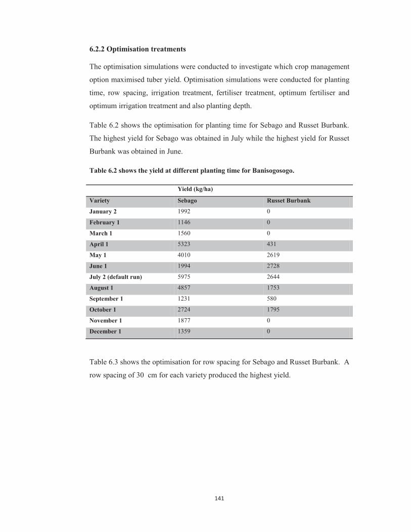
141
6.2.2 Optimisation treatments
The optimisation simulations were conducted to investigate which crop management
option maximised tuber yield. Optimisation simulations were conducted for planting
time, row spacing, irrigation treatment, fertiliser treatment, optimum fertiliser and
optimum irrigation treatment and also planting depth.
Table 6.2 shows the optimisation for planting time for Sebago and Russet Burbank.
The highest yield for Sebago was obtained in July while the highest yield for Russet
Burbank was obtained in June.
Table 6.2 shows the yield at different planting time for Banisogosogo.
Yield (kg/ha)
Variety Sebago Russet Burbank
January 2 1992 0
February 1 1146 0
March 1 1560 0
April 1 5323 431
May 1 4010 2619
June 1 1994 2728
July 2 (default run) 5975 2644
August 1 4857 1753
September 1 1231 580
October 1 2724 1795
November 1 1877 0
December 1 1359 0
Table 6.3 shows the optimisation for row spacing for Sebago and Russet Burbank. A
row spacing of 30 cm for each variety produced the highest yield.
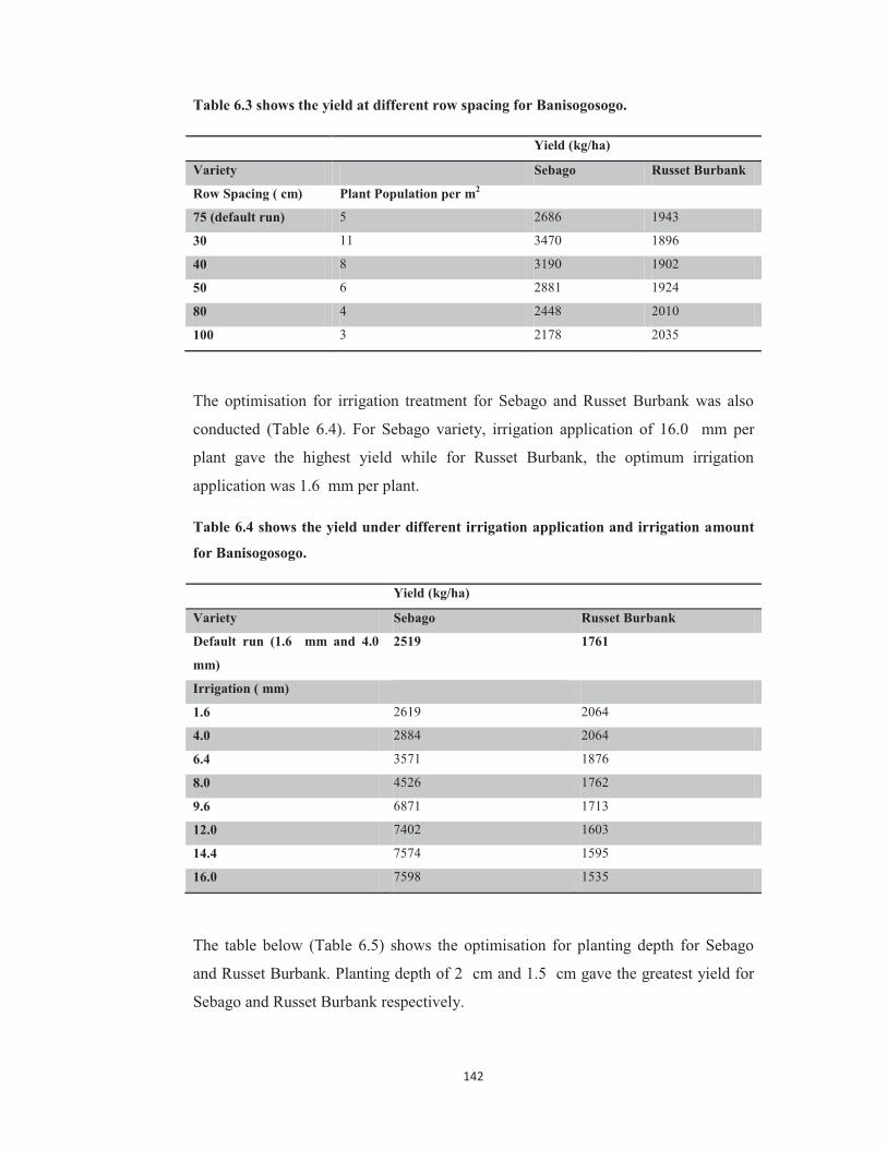
142
Table 6.3 shows the yield at different row spacing for Banisogosogo.
Yield (kg/ha)
Variety Sebago Russet Burbank
Row Spacing ( cm) Plant Population per m2
75 (default run) 5 2686 1943
30 11 3470 1896
40 8 3190 1902
50 6 2881 1924
80 4 2448 2010
100 3 2178 2035
The optimisation for irrigation treatment for Sebago and Russet Burbank was also
conducted (Table 6.4). For Sebago variety, irrigation application of 16.0 mm per
plant gave the highest yield while for Russet Burbank, the optimum irrigation
application was 1.6 mm per plant.
Table 6.4 shows the yield under different irrigation application and irrigation amount
for Banisogosogo.
Yield (kg/ha)
Variety Sebago Russet Burbank
Default run (1.6 mm and 4.0
mm)
2519 1761
Irrigation ( mm)
1.6 2619 2064
4.0 2884 2064
6.4 3571 1876
8.0 4526 1762
9.6 6871 1713
12.0 7402 1603
14.4 7574 1595
16.0 7598 1535
The table below (Table 6.5) shows the optimisation for planting depth for Sebago
and Russet Burbank. Planting depth of 2 cm and 1.5 cm gave the greatest yield for
Sebago and Russet Burbank respectively.

143
Table 6.5 shows the planting depth with corresponding yield for Banisogosogo.
Yield (kg/ha)
Variety Sebago Russet Burbank
Planting Depth ( cm)
1.5 (default run) 2686 1943
2 3011 1696
4 2739 453
6 1846 325
8 2686 0
10 2686 0
Table 6.6 shows the optimisation for fertiliser treatment for Sebago variety. The
highest yield for Sebago was obtained using 300 kg/ha at 10 cm. The results also
indicated that the yield obtained for optimum fertiliser and optimum irrigation
simulation was higher than default value and optimised irrigation yield but lower
than optimised fertiliser yield (Table 6.7).
Table 6.6 shows the application of fertiliser (banded beneath surface) and
corresponding yield for Banisogosogo for Sebago variety.
Yield (kg/ha) at depth
Default run (80 N kg/ha in
2 splits at 5 cm)
2577
Fertiliser (kg/ha) 0 cm 2 cm 4 cm 6 cm 8 cm 10 cm
60 2579 2579 2579 2652 2758 2826
120 2622 2622 2622 2787 3004 3136
180 2640 2640 2640 2895 3241 3409
240 2646 2646 2646 2992 3432 3671
300 2648 2648 2648 3109 3607 4359
Table 6.7 shows the optimum fertiliser and irrigation management for Banisogosogo
for Sebago variety.
Fertiliser Application (kg/ha at 10 cm) Irrigation Application ( mm) Yield (kg/ha)
300 kg/ha 16.0 2645

144
The table below shows the optimisation for fertiliser treatment for Russet Burbank
variety (Table 6.8). The highest yield for Russet Burbank was obtained using 300
kg/ha under 0-4 cm. Under the optimum fertiliser and optimum irrigation treatments,
the yield obtained was higher than the default value but lower than the optimum
fertiliser yield (Table 6.9).
Table 6.8 shows the application of fertiliser (banded beneath surface) and
corresponding yield for Banisogosogo for Russet Burbank.
Yield (kg/ha) at depth
Default run (80 N kg/ha in
2 splits at 5 cm)
1990
Fertiliser (kg/ha) 0 cm 2 cm 4 cm 6 cm 8 cm 10 cm
60 1915 1915 1915 1903 1888 1877
120 2008 2008 2008 1995 1837 1778
180 2369 2369 2369 2400 2256 2033
240 2402 2402 2402 2305 2132 2126
300 2420 2420 2420 2173 2018 1999
Table 6.9 shows the optimum fertiliser and irrigation management for Banisogosogo
for Russet Burbank.
Fertiliser Application (kg/ha at x cm) Irrigation Application ( mm) Yield (kg/ha)
300 at 0 cm 1.6 1959
300 at 2 cm 1.6 2381
300 at 4 cm 1.6 2381
300 at 0 cm 4.0 1923
300 at 2 cm 4.0 2348
300 at 4 cm 4.0 0
6.2.3 Climate variability (El Niño Southern Oscillation) simulation
The impact of climate variability was also studied on Sebago and Russet Burbank
potato yield for Banisogosogo. Differences in the yield were noticed during El Niño,
La Niña and neutral years. For Sebago cultivar, average El Niño years gave the
lowest yield (7 year average) at 2124 kg/ha (percentage difference 63.43%) while La
Niña produced an average yield of 2883.43 kg/ha at 34.77 % (Table 6.11). On the
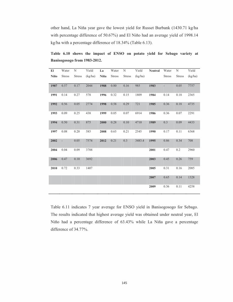
145
other hand, La Niña year gave the lowest yield for Russet Burbank (1430.71 kg/ha
with percentage difference of 50.67%) and El Niño had an average yield of 1998.14
kg/ha with a percentage difference of 18.34% (Table 6.13).
Table 6.10 shows the impact of ENSO on potato yield for Sebago variety at
Banisogosogo from 1983-2012.
El
Niño
Water
Stress
N
Stress
Yield
(kg/ha)
La
Niña
Water
Stress
N
Stress
Yield
(kg/ha)
Neutral Water
Stress
N
Stress
Yield
(kg/ha)
1987 0.57 0.17 2044 1988 0.80 0.16 985 1983 - 0.05 7757
1991 0.14 0.27 578 1996 0.32 0.15 1809 1984 0.14 0.18 2365
1992 0.56 0.05 2774 1998 0.58 0.29 721 1985 0.36 0.18 4735
1993 0.09 0.25 438 1999 0.05 0.07 6914 1986 0.36 0.07 2291
1994 0.50 0.31 875 2000 0.28 0.10 4710 1989 0.3 0.09 4433
1997 0.08 0.20 585 2008 0.65 0.21 2545 1990 0.17 0.11 6368
2002 - 0.05 7574 2012 0.21 0.3 3483.4 1995 0.86 0.34 708
2004 0.04 0.09 3788 2001 0.47 0.2 2960
2006 0.47 0.10 3692 2003 0.45 0.26 759
2010 0.72 0.33 1407 2005 0.31 0.16 2085
2007 0.65 0.14 1328
2009 0.36 0.11 4258
Table 6.11 indicates 7 year average for ENSO yield in Banisogosogo for Sebago.
The results indicated that highest average yield was obtained under neutral year, El
Niño had a percentage difference of 63.43% while La Niña gave a percentage
difference of 34.77%.

146
Table 6.11 shows the 7 year average for ENSO yield for Banisogosogo for Sebago
variety. The highest yield was obtained by the neutral years.
7 Year Average Yield (kg/ha) Percentage Difference
(%)
El Niño (1987-2002) 2124 63.43
La Niña (1988-2012) 2883.43 34.77
Neutral Year (1983- 1995) 4096.86
Table 6.12 shows the yield obtained under each ENSO state and water and nitrogen
stress faced during the ENSO state. Russet Burbank variety appeared to be more
stable variety for El Niño years.
Table 6.12 shows the impact of ENSO on potato yield for Banisogosogo for Russet
Burbank from 1983-2010.
El Niño
Water Stress
N Stress
Yield (kg/ha)
La Niña
Water Stress
N Stress
Yield (kg/ha)
Neutral Water Stress
N Stress
Yield (kg/ha)
1987 0.65 0.23 2151 1988 1.00 0.33 292 1983 - 0.02 1786
1991 0.43 0.30 1243 1996 0.32 0.18 2526 1984 0.48 0.28 1658
1992 0.70 0.13 1070 1998 0.73 0.33 698 1985 0.35 0.12 1323
1993 0.10 0.25 543 1999 0.03 0.03 1497 1986 0.35 0.16 2700
1994 0.59 0.31 1055 2000 0.29 0.22 2355 1989 0.31 0.21 4381
1997 0.07 0.17 2152 2008 0.82 0.32 402 1990 0.14 0.14 4434
2002 - 0.06 5773 2012 0.19 0.17 2245 1995 1.00 0.55 530
2004 - 0.07 6746 2001 0.59 0.17 1996
2006 0.53 0.08 3939 2003 0.59 0.28 973
2010 1.00 0.40 1172 2005 0.44 0.18 2727
2007 0.87 0.30 339
2009 0.27 0.34 1689
Table 6.13 indicates 7 year average for ENSO yield in Banisogosogo for Russet
Burbank. The results indicated that highest average yield was obtained under neutral
year, the percentage difference for El Niño was 18.34% while La Niña gave a
percentage difference of 50.67%.

147
Table 6.13 shows 7 year average for ENSO yield for Banisogosogo for Russet Burbank.
The highest yield was obtained under neutral year.
7 Year Average Yield (kg/ha) Percentage Difference
(%)
El Niño (1987-1997) 1998.14 18.34
La Niña (1988-2008) 1430.71 50.67
Neutral Year (1983- 1990) 2401.7
6.2.2 Future climate simulations
The impacts of future climatic scenario on Sebago and Russet Burbank were
simulated in Banisogosogo using DSSAT SUBSTOR Potato model. In this study two
PSSCP climate scenarios were used (similar to Chapter 5). The results are divided
into two sections; (i) the future climate simulations with potential and non-potential
production and (ii) the optimisation treatments.
6.2.2.1 Banisogosogo Sebago simulation
For Banisogosogo potential simulations (Table 6.14), under future emission scenario,
the tuber initiation day and LAI increased while the tuber fresh and dry weight
decreased. However, there was no tuber production noted under 2090 potential
simulation. It was also noticed that the tuber initiation day was earlier for non-
potential simulation as compared to potential simulation. The LAI values for non-
potential simulation were lower when compared to potential simulation.
Table 6.14 shows the Banisogosogo future climate simulation for Sebago variety. 2030 2055 2090 Potential Non-Potential Potential Non-Potential Potential Non-Potential Variable Medium High Medium High Medium High Medium High Medium High Medium High Tuber Initiation Day (dap)
41 39 39 37 53 51 52 47 -99 -99 57 -99
Tuber Dry Weight (kg\ha) harvest
4835 5511 2947 3703 2068 3333 1485 2566 0 0 19 0
Tuber Fresh Weight (t\ha) harvest
24.17 27.56 14.73 18.52 10.34 16.66 7.42 12.83 0 0 0.09 0
Leaf Area Index
6.13 6.12 2.37 2.43 9.33 11.46 4.55 4.71 22.05 23.87 6.93 8.33

148
Figure 6.4 shows Banisogosogo future climate potential simulations for Sebago for LAI, leaf
weight, stem weight, tuber dry and fresh weight and tops weight.
The above simulation indicates that tuber dry yield (e) and tuber fresh weight (f) was
only possible for 2030-2055 A1B and A2 emission scenario. The above figure also
shows that the highest tuber yields were obtained under 2030 A1B and A2 emission
scenario. On the other hand, 2030 A1B and A2 emission scenario, gave the lowest
a) LAI b) Leaf weight
c) Stem weight d) Tops weight
e) Tuber dry weight f) Tuber fresh weight

149
value for LAI, leaf weight and stem weight (a, b, c, and d respectively) while
vegetative growth was highest for 2090 A1B and A2 emission scenario.
Figure 6.5 shows Banisogosogo future climate non-potential simulations for Sebago for LAI,
leaf weight, stem weight, tuber dry and fresh weight and tops weight.
a) LAI b) Leaf weight
c) Stem weight d) Tops weight
e) Tuber dry weight f) Tuber fresh weight
150
The above figure illustrates that tuber dry weight (e) and tuber fresh weight (f) under
non-potential simulation was possible for 2030-2055 A1B and A2 emission scenarios
and 2090 A2 emission scenario. However, the yield for 2090 A2 emission scenario
was very low.
6.2.2.2 Optimisation treatments
The optimisation treatment was conducted for non-potential simulation for Sebago
and Russet Burbank to investigate which crop management strategies maximised the
tuber yield under future climate scenario. Optimisation simulation was conducted for
planting time, row spacing, irrigation treatment, fertiliser treatment, optimum
fertiliser and optimum irrigation treatment and also planting depth. The results
suggest that under each emission scenario different crop management practices
optimise the yield (Table 6.15 and Table 6.17).
The Banisogosogo optimisation treatment showed that under 2030 AIB and A2
emission scenario, the optimum planting time was June while for 2055 AIB and A2
and 2090 A1B emission scenario, the optimum planting time was July. The optimum
row spacing for 2030 A1B and A2 was 30 cm whereas the optimum row spacing for
2055 A1B and A2 was 40 cm and 100 cm respectively. The optimum row spacing
for 2090 A1B was 30 cm. Under 2030 A1B and A2 emission scenario, 6.4 mm
irrigation produced the highest yield but for 2055 and 2090 A1B emission scenario,
1.6 mm irrigation gave the highest yield. The optimisation treatment for fertiliser for
2030 A1B and A2 emission scenario indicated that application of 300 kg/ha fertiliser
at 10 cm and application of 300 kg/ha fertiliser at 8 cm simulated the highest yield
respectively. In 2055 A1B and A2 emission scenario, the optimum fertiliser
application was 300 kg/ha fertiliser at 0-4 cm while in 2090 A1B emission scenario,
the optimum fertiliser application was 60 kg/ha fertiliser at 0-4 cm. The optimum
fertiliser and the optimum irrigation application indicated that the yield was not
optimised for 2030 and 2055 A1B and A2 emission scenario. However, the optimum
fertiliser and the optimum irrigation application did optimise the yield for 2090 A1B
emission scenario. Under 2030-2055 A1B and A2 and 2090 A1B emission scenario,
the optimum planting depth was 1.5 cm.

151
Table 6.15 shows the optimisation treatments for Sebago.
Optimum Treatment, Yield (kg/ha) Banisogosogo 2030 A1B
Emission 2030 A2 Emission
2055 A1B Emission
2055 A2 Emission
2090 A1B Emission
Planting Time June, 5004 June, 6085 July, 2840 July, 4015 July, 597 Row Spacing 30 cm, 2988 30 cm, 4081 40 cm, 1493 100 cm, 2603 30 cm, 18 Irrigation Application
6.4 mm, 5251 6.4 mm, 6465 1.6 mm, 1673 1.6 mm, 2656 1.6 mm, 20
Fertiliser Application
300 kg/ha fertiliser at 10 cm, 4256
300 kg/ha fertiliser at 8, 5367
300 kg/ha fertiliser at 0-4 cm, 2241
300 kg/ha fertiliser at 0-4 cm, 3089
60 kg/ha fertiliser at 0-4 cm, 38
Optimum Irrigation and Fertiliser Application
4641 5749 2211 3130 911
Planting Depth 1.5 cm, 2947 1.5 cm, 3703 1.5 cm, 1485 1.5 cm, 2566 1.5 cm, 17
6.2.2.3 Russet Burbank variety simulations
For Banisogosogo Russet Burbank potential simulations (Table 6.16) tuber yield was
only possible under 2030 A2 non-potential simulations. Tuber dry weight obtained
under this scenario was 37 kg/ha while the tuber fresh weight obtained was 0.19 t/ha.
However, this tuber yield was negligible. The LAI under all emission scenarios was
very high. Figures 6.6 and 6.7 represent the same tabulated information. These
graphs show that under potential and non-potential simulation there was very high
vegetative or above-ground growth.
Table 6.16 shows Banisogosogo simulation results of future climate simulation for
Russet Burbank Variety for A1B and A2 emission scenario. 2030 2055 2090 Potential Non-
Potential Potential Non-
Potential Potential Non-
Potential Variable A1B A2 A1B A2 A1B A2 A1B A2 A1B A2 A1B A2 Tuber Initiation Day (dap)
-99 -99 -99 74 -99 -99 -99 -99 -99 -99 -99 -99
Tuber Dry Weight (kg\ha) harvest
0 0 0 37 0 0 0 0 0 0 0 0
Tuber Fresh Weight (t\ha) harvest
0 0 0 0.19 0 0 0 0 0 0 0 0
Leaf Area Index
19.14 19.76 9.70 9.26 19.01 24.64 9.01 10.32 19.08 20.65 7.55 7.75
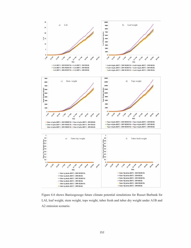
152
Figure 6.6 shows Banisogosogo future climate potential simulations for Russet Burbank for
LAI, leaf weight, stem weight, tops weight, tuber fresh and tuber dry weight under A1B and
A2 emission scenario.
a) LAI b) Leaf weight
c) Stem weight d) Tops weight
e) Tuber dry weight f) Tuber fresh weight
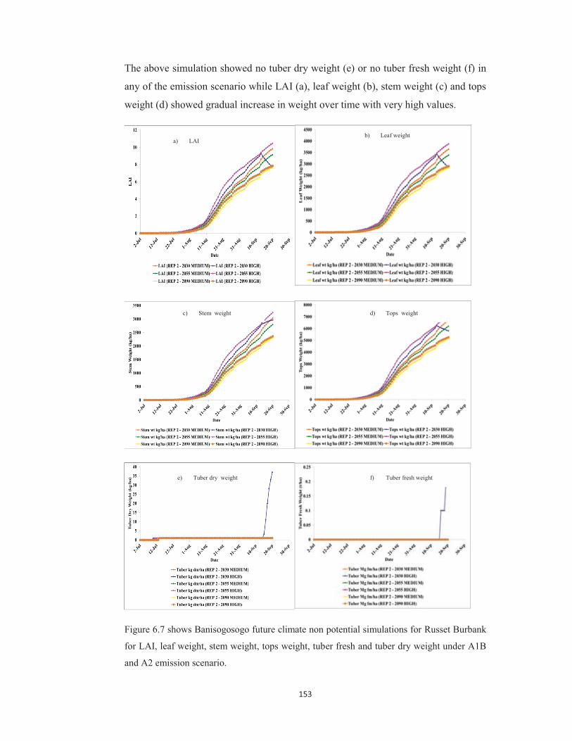
153
The above simulation showed no tuber dry weight (e) or no tuber fresh weight (f) in
any of the emission scenario while LAI (a), leaf weight (b), stem weight (c) and tops
weight (d) showed gradual increase in weight over time with very high values.
Figure 6.7 shows Banisogosogo future climate non potential simulations for Russet Burbank
for LAI, leaf weight, stem weight, tops weight, tuber fresh and tuber dry weight under A1B
and A2 emission scenario.
a) LAI b) Leaf weight
c) Stem weight d) Tops weight
e) Tuber dry weight f) Tuber fresh weight
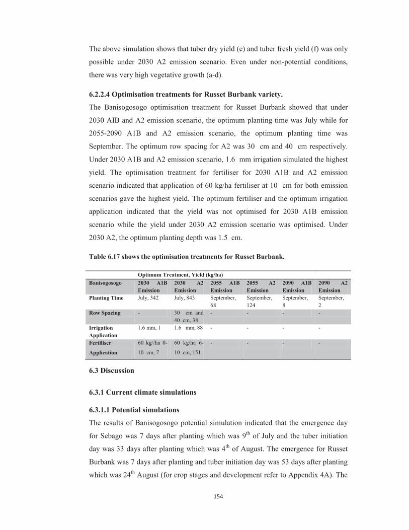
154
The above simulation shows that tuber dry yield (e) and tuber fresh yield (f) was only
possible under 2030 A2 emission scenario. Even under non-potential conditions,
there was very high vegetative growth (a-d).
6.2.2.4 Optimisation treatments for Russet Burbank variety.
The Banisogosogo optimisation treatment for Russet Burbank showed that under
2030 AIB and A2 emission scenario, the optimum planting time was July while for
2055-2090 A1B and A2 emission scenario, the optimum planting time was
September. The optimum row spacing for A2 was 30 cm and 40 cm respectively.
Under 2030 A1B and A2 emission scenario, 1.6 mm irrigation simulated the highest
yield. The optimisation treatment for fertiliser for 2030 A1B and A2 emission
scenario indicated that application of 60 kg/ha fertiliser at 10 cm for both emission
scenarios gave the highest yield. The optimum fertiliser and the optimum irrigation
application indicated that the yield was not optimised for 2030 A1B emission
scenario while the yield under 2030 A2 emission scenario was optimised. Under
2030 A2, the optimum planting depth was 1.5 cm.
Table 6.17 shows the optimisation treatments for Russet Burbank.
Optimum Treatment, Yield (kg/ha) Banisogosogo 2030 A1B
Emission 2030 A2 Emission
2055 A1B Emission
2055 A2 Emission
2090 A1B Emission
2090 A2 Emission
Planting Time July, 342 July, 843 September, 68
September, 124
September, 8
September, 2
Row Spacing - 30 cm and 40 cm, 38
- - - -
Irrigation Application
1.6 mm, 1 1.6 mm, 88 - - - -
Fertiliser
Application
60 kg//ha 0-
10 cm, 7
60 kg/ha 6-
10 cm, 151
- - - -
6.3 Discussion
6.3.1 Current climate simulations
6.3.1.1 Potential simulations
The results of Banisogosogo potential simulation indicated that the emergence day
for Sebago was 7 days after planting which was 9th of July and the tuber initiation
day was 33 days after planting which was 4th of August. The emergence for Russet
Burbank was 7 days after planting and tuber initiation day was 53 days after planting
which was 24th August (for crop stages and development refer to Appendix 4A). The

155
tuber fresh weight for Sebago and Russet Burbank was 38.88 t/ha and 14.43 t/ha with
tuber dry weight as 7777 kg/ha and 2885 kg/ha respectively (refer to Table 6.1). The
leaf area index for Sebago was 6.14 while for Russet Burbank it was 8.44. As shown
in Figure 6.0 for Sebago, LAI, leaf weight, stem weight, tops weight, tuber fresh and
tuber dry weight increased steadily with time. Figure 6.1 indicated that the LAI and
leaf weight for Russet Burbank increased initially and decreased after 23rd of August.
The tuber fresh weight started to increase around 23rd of August. The drop in LAI
and leaf weight can be due to transfer of photosynthate from the leaves to the tubers.
For Russet Burbank, tuber initiation occurred during early flowering (Dwelle and
Love, 1993), the maximum bulking rate has been recorded at 7-8 cwt/A-day and
under optimum growing conditions, the tuber bulking rate is linear from tuber
initiation until maturity or leaf senescence (Kleinkopf et al., 2003).
6.3.1.2 Non-potential simulation
The Banisogosogo Sebago non-potential simulation indicated that the emergence day
was 7 days after planting which was 9th of July. The tuber initiation day was 31 days
after planting which was 2nd of August. Under non-potential conditions the tuber
fresh weight was 13.43 t/ha while the tuber dry weight was 2686 kg/ha with leaf area
index of 0.45. As shown by Figure 6.0, LAI, leaf weight, stem weight and tops
weight all increased from the day of planting until 3rd of August from which there
was a decline in LAI and leaf weight, stem weight and tops weight. On the other
hand, there was an increase in tuber dry and fresh weight after 3rd of August. This
can be due to the transfer of photosynthetic product from the above ground to below
ground. There was also evidence of nitrogen stress on 2nd August and water and
nitrogen stress on 20th September. Figure 6.2 indicated that there was gradual
increase in precipitation and total nitrate rate over time. The increase in total nitrate
can be due to application of nitrogen fertilisers on 7th and 23rd of July. Furthermore,
it also showed that the total nitrate available in the soil increased few days after the
application of fertilisers. This can be due to onset of plant senescence or decay of
aboveground components, such as, leaves and stems, as tubers reached maturity. On
the other hand, Russet Burbank emerged 7 days after planting (9th July). In Russet
Burbank, aged seed accounted for earlier emergence along with an increase of stem
number per plant. However, the seed age did not affect the overall yield (Olsen and
Nolte, 2004). Table 6.1 indicated that the tuber initiation day was 50 days after

156
planting which was 21st of August with tuber fresh weight of 9.61 t/ha, leaf area
index of 5.88 and tuber dry weight of 1922 kg/ha. The optimum soil temperature for
Russet Burbank tuber growth is 16 ºC while the optimum temperature for vine
growth is 25 ºC. At higher temperatures, tuber growth is delayed (Dwelle and Love,
1993). At temperatures of 15 ºC and 24 ºC, Russet Burbank and White Rose, had
higher yield, high starch content and high specific gravity as compared to higher
temperatures (Yamaguchi et al., 1964). Figure 6.1 indicated that LAI, leaf weight
and tops weight increased from the planting day until 30th of August after which it
showed fluctuation in weight and then increased gradually with time. On the other
hand, there was an increase in tuber dry and fresh weight after 23rd of August.
Translocation for Russet Burbank from vine to tubers may account for 10-15 % of
the final yield (Kleinkopf et al., 2003). Figure 6.3 also showed an increase in total
nitrate rate due to application of fertilisers (on 7th and 23rd of July nitrogen fertiliser
was applied which also shows an increase in nitrate rate). However, there was a
decline in nitrate rate and total water content in the soil around 10th of August and the
harvest date. It was seen that the crop underwent water stress on 20th of September
and nitrogen stress on 21st August and 20th September.
It was also noticed from the simulations that there is a huge difference between
potential and non-potential yields for both the varieties. Under potential production,
maximum production was reported with no indication of water and nitrogen stress.
While under non-potential production, the crop was sensitive to water and nitrogen
stress which reduced the crop’s performance and yield.
6.3.1.3 Optimisation treatment
To begin with, optimisation was conducted for planting time to see which month
gave the highest tuber yield. The optimisation for planting time, as shown by Table
6.2, indicated that planting of Sebago variety in Banisogosogo during the month of
July produced the highest yield (5975 kg/ha). This was because the month of July
gave the low average maximum and minimum temperature with adequate rainfall
from planting to harvest. On the other hand, Russet Burbank should be planted in
June which produced tuber dry weight of 2728 kg/ha. The month of June gave the
lowest average maximum and minimum temperature. The results also indicated that
for cultivar Russet Burbank, the months of January, February, March, November and
December produced no tuber. This was because these months had no tuber initiation
157
development phase. As mentioned earlier, low temperature is necessary for tuber
initiation. For cultivar Russet Burbank, which requires more time for tuber initiation,
planting should take place earlier (June) as compared to Sebago (July). Planting too
early in the season can lead to slow emergence, decreased plant vigor, slow tuber
growth rate and susceptibility to seed disease while planting too late in the season
delays canopy development and reduces time available for tuber bulking (Dwelle and
Love, 1993).
Row spacing was also optimised and the yield obtained under each treatment was
noted. The optimisation results for Sebago for Banisogosogo for row spacing
indicated that a row spacing of 30 cm gave the highest yield at 3470 kg/ha. On the
other hand, Russet Burbank simulation in Banisogosogo indicated that a row spacing
of 100 cm produced the highest yield (Table 6.3). Planting closer to optimum reduces
photosynthetic capacity for bulking giving rise to smaller tubers and lower
marketable yields while planting wider than the optimal row spacing can lengthen
the time for full canopy development reducing carbohydrate supply to tubers (Dwelle
and Love, 1993).
Likewise, optimisation was conducted for irrigation application. Banisogosogo
optimisation treatment for irrigation for Sebago indicated that increasing the
irrigation level increased the tuber yield. Hence, the highest tuber yield was obtained
at 16 mm of irrigation while the lowest tuber yield was obtained at 1.6 mm. The
yield of Sebago variety can be increased by maintaining high but safe soil moisture
content throughout the potato growing season (Myhre, 1956). On the other hand, for
Russet Burbank simulation, application of 1.6 mm and 4.0 mm of irrigation per plant
gave the highest yield at 2064 kg/ha (Table 6.4). Water stress can delay the
appearance of particular order of apical branches, the production rate of new leaves,
enhance leaf senescence and there is slowed maturation and compensatory leaf
production upon recovery from transient water stress. As compared to water treated
plants, drought treated plants produced less leaf area 50-83 days after planting (Vos
and Haverkort, 2007b).
The optimisation simulation for Banisogosogo planting depth indicated that planting
of Sebago variety at a depth of 2 cm produced the highest tuber yield (3011 kg/ha).
The lowest tuber yields was obtained at 6 cm (1846 kg/ha) while planting depth of
158
1.5 cm, 6 cm and 8 cm gave the similar tuber yield of 2686 kg/ha. The simulation for
Russet Burbank indicated that increasing the planting depth decreased the tuber yield
(Table 6.5). Planting of Russet Burbank at great depths such as 9 inches (22.86 cm)
greatly reduced tuber yield (Bohl, 2006).
Furthermore, fertiliser treatment was also optimised. As indicated by Table 6.6, the
Banisogosogo fertiliser results for Sebago showed that application of 300 kg/ha
fertiliser at 10 cm gave the highest yield at 4359 kg/ha. Application of fertiliser at 0
cm, 2 cm and 4 cm gave similar yield. On the other hand, Russet Burbank simulation
showed that application of 300 kg/ha fertiliser at 0 cm, 2 cm and 4 cm gave the
highest yield at 2420 kg/ha (Table 6.8). It was also noticed that the yield obtained
under 0-4 cm was similar. This is because surface application (0 cm) will be similar
to application up to top layer soil. The model will show very little or no difference
between first soil layer (0-5 cm) applications. However, at 6 cm soil layer, the model
starts to show difference. For Russet Burbank, LAI of 3.0-3.5 maximises the
interception of sunlight. Under excessive nitrogen fertiliser application for Russet
Burbank, there is increase in vine size above the necessary to maximise the bulking
rate. However, under excessive nitrogen fertiliser application, there is delay in tuber
initiation as much as 10 to 14 days which can reduce yield as much as 90 cwt/A
(Kleinkopf et al., 2003).
Finally optimisation was conducted for optimum fertiliser and optimum irrigation
treatments. When optimum fertiliser application and the optimum irrigation levels for
Sebago and Russet Burbank were combined as a treatment for simulation, the results
suggested that the yield of tuber obtained under this simulation was higher than
default value and optimised irrigation yield but lower than optimised fertiliser yield.
For impacts of ENSO on potato yield simulation neutral year gave the highest tuber
yield for both varieties. For Sebago variety (Table 6.11), average El Niño years gave
the lowest yield (7 year average) at 2124 kg/ha (percentage difference of 63.43%)
while La Niña gave an average yield of 2883.43 kg/ha (percentage difference of
34.77%). El Niño years gave the lowest yield because the crop underwent a lot of
water stress as compared to other ENSO phase (as shown in Table 6.10). On the
other hand, for Russet Burbank variety, La Niña year gave the lowest yield at
1430.71 kg/ha with percentage difference of 50.67% and El Niño gave an average

159
yield of 1998.14 kg/ha with a percentage difference of 18.34% (Table 6.13). As
shown by Table 6.12, La Niña years faced a lot of nitrogen stress which could be one
reason for the low yield obtained. Overall, it can be said that Russet Burbank was a
more stable variety for El Niño events.
6.3.2 Future climate simulation
6.3.2.1 Potential simulations
Banisogosogo Sebago potential simulation (Table 6.14) for 2030 medium emission
scenario indicated that the emergence day was 10th of July (8 days after planting),
tuber initiation day was 12th of August, that is, 41 days after planting. Table 6.14
indicated that the tuber dry weight was 4835 kg/ha with 24.17 t/ha of tuber fresh
weight with LAI of 6.13. For 2030 high emission scenario the results showed that the
emergence day was 10th of July, tuber initiation day was 39 days after planting, that
is, 10th of August, with tuber dry weight of 5511 kg/ha and tuber fresh weight of
27.56 t/ha with LAI of 6.12. The simulation for 2030 high emission scenario showed
that the tuber initiation was 2 days earlier with higher tuber dry and tuber fresh
weight. One reason for this can be the difference in annual temperature increase and
precipitation level in each scenario, that is, 2030 high emission scenario had low
annual temperature increase with higher level of precipitation as compared to 2030
medium emission scenario. Under 2055 medium emission scenario, the emergence
day was 11th of July, tuber initiation day was 53 days after planting, that is 34th of
August, with tuber dry weight of 2068 kg/ha and tuber fresh weight of 10.34 t/ha and
LAI of 9.33. For 2055 high emission scenario, it was seen that the emergence day
was 11th of July, tuber initiation day was 51 days after planting, that is, 22nd of
August. The tuber dry weight was 3333 kg/ha with tuber fresh weight of 16.66 t/ha
with LAI 11.46. There was no tuber yield under 2090 medium and high emission
scenario. As shown by Figure 6.4, under 2030 and 2090 medium and high emission
scenario, the LAI, leaf weight, stem weight and tops weight increased with time
while under 2055 medium and high emission scenario, the LAI increased from the
planting date until the 23rd of August and 21st of August respectively. The tuber
weight increased gradually from 15th August, 11th August, 26th August, 23rd August
for 2030 medium emission, 2030 high emission, 2055 medium emission and 2055
high emission respectively. The figure also showed that 2090 medium emissions had
high vegetative growth while the highest tuber fresh and dry yield was shown by

160
2030 high emission followed by 2030 medium emission, 2055 high emission and
2055 medium emission. On the other hand, it was seen that Russet Burbank under all
emission scenario, the yield was zero with very high vegetative growth and LAI
(Table 6.16 and Figure 6.4).
6.3.2.2 Non potential simulations
Banisogosogo non potential simulations for Sebago for 2030 medium emission
scenario indicated that the emergence day was 11th of July, tuber initiation day was
10th of August (39 days after planting) with tuber dry weight of 2947 kg/ha and tuber
fresh weight of 14.73 t/ha and LAI of 2.37. Water stress was seen on the 20th of
September and nitrogen stress on the 10th of August and 20th of September. For 2030
high emission scenario it was seen that the emergence date was 10th of July, tuber
initiation day was 8th of August (37 days after planting). The harvest for dry weight
was 3703 kg/ha with harvest of fresh weight of 18.52 t/ha and LAI of 2.43. The crop
faced water and nitrogen stress on 8th of August and 20th of September. Availability
of soil nutrients and moisture determines not only the number but also the quality of
tubers that reach maturity (Food and Agricultural Organisation of the United
Nations, 2008). Under elevated carbon dioxide there is limited transpiration which
leads to decreased nitrogen uptake and chlorophyll loss (Bindi et al., 2002). It can be
also seen that the 2030 high emission had an earlier tuber initiation day with higher
dry and fresh tuber yield. Under 2055 medium emission scenario, the emergence day
was 12th of July with tuber initiation at 23rd of August (52 days after planting). The
tuber dry weight was 1485 kg/ha and tuber fresh weight was 7.42 t/ha and LAI of
4.55. It was seen that the crop underwent water and nitrogen stress on 23rd of August
and 20th of September. Furthermore, 2055 high emission scenario indicated that the
emergence day was 11th of July, tuber initiation day was 18th of August (47 days
after planting) with tuber dry weight at 2566 kg/ha, tuber fresh weight at 12.83 t/ha
and LAI of 4.71. The crop underwent water stress on the 20th of September and
nitrogen stress on 18th of August and 20th of September. It can also been seen that
the tuber initiation day increased and the tuber dry weight and fresh weight decreased
under 2055 emission scenario as compared to 2030 emission scenario. For 2090
medium emission scenario, the emergence day was 14th of July, tuber initiation day
was 14th of September (74 days after planting). This emission scenario had very little
tuber yield, with tuber dry weight at 19 kg/ha, tuber fresh weight at 0.09 t/ha and LAI
161
of 6.93. The crop underwent water and nitrogen stress on 14th and 20th of September
respectively. Under 2090 high emission scenario, the emergence day was 14th of
July. However, there was no tuber initiation. Figure 6.5 indicated that LAI, leaf
weight, stem weight and tops weight increased from the day of planting but
experienced a decline in weight on 31st of August, 8th and 13th of September. The
tuber weight increased from 11th of August, 9th of August, 26th of August, 20th of
August for 2030 medium, 2030 high, 2055 medium and 2055 high emission scenario
respectively. The LAI, leaf weight, stem weight and the tops weight were the highest
for 2090 medium emission scenario followed by 2055 high emission scenario, 2055
medium emission scenario, 2030 high emission scenario and 2030 medium emission
scenario. The tuber fresh weight and tuber dry weight indicated that the highest yield
were obtained under 2030 high emission scenario followed by 2030 medium
emission scenario, 2055 high emission scenario, 2055 medium and 2090 medium
emission scenario. Warm temperatures favour vegetative growth while cool
temperature favour tuber growth (Ewing, 1981c; Khedher and Ewing, 1985). On the
other hand, Russet Burbank can only be cultivated under 2030 high emission
scenario. This emission scenario produced negligible yield. The emergence date
under this emission scenario was 10th of July (8 days after planting) with tuber dry
weight of 37 kg/ha, tuber fresh weight of 0.19 t/ha and LAI of 9.26. Under all other
emission scenario, it was observed that there was high LAI but no tuber yield (Table
6.16). Figure 6.7 indicated that under 2030 high emission scenario, the LAI increased
from the day of planting until 13th of September. After 13th of September until the
day of harvest there was a decline in LAI value. For all other scenarios, the LAI
increased gradually with time. The tuber fresh weight for 2030 high emission
scenario increased from 13th of September until 16th of September. From 16th of
September to 17th of September there was no gain in weight. The tuber weight
increased again from 18th of September to the day of harvest. The crop faced water
and nitrogen stress on 20th of September. Finally, it can be said that Sebago was the
best variety to be cultivated in Banisogosogo. The effect of elevated temperature on
potato growth and yield is determined by a combination of factors, such as, between
soil temperature, air temperature, solar radiation and photoperiod (Sarquis et al.,
1996). For Sebago, it was noted that high temperature (32 oC/28 oC, day/night)
promote haulm growth and suppress tuber production (Menzel, 1980, 1983a). At
elevated temperatures dry matter is diverted to shoots rather than tubers (Menzel,

162
1985). Correspondingly, at high shoot and root temperatures tuber formation is
strongly inhibited. Disbudding promoted tuberisation at such cases (Menzel, 1983b).
The yield of potatoes should increase by 10% for every extra 100 ppm CO2 (Bindi,
2008). Under 28 oC and 30 oC, there was a delay in tuber formation for Desiree and
Russet Burbank (Nowak and Colborne, 1989). When Russet Burbank was grown
under 350 of 1000 µmol mol-1, irradiance of 400 or 800µE m-2s-1 photosynthetic
photon flux and photoperiod of 12 or 24 hours, it was seen that tuber yield increased
at elevated carbon dioxide but at lower photosynthetic photon flux (Pereira and C.C.
Shock, 2006). Similarly, another study shows that Russet Burbank tuber yield were
highest at low temperature of 17.5oC, carbon dioxide concentration of 1600µL L-1
and medium light of 455 µmol m-2s-1 (Yandell et al., 1988). The effect of
temperature (25 oC/12 oC and 35 oC/25 oC) on dry matter production of Russet
Burbank, Desiree and DTO-28 was studied for five week, 2 week after tuberisation.
The study showed that tuber growth rate was more affected by high temperature than
the whole plant. The study also showed that all varieties experienced a decline in
tuber dry matter production at high temperature as compared to low temperature with
Russet Burbank experiencing the largest decline (Thornton et al., 1996). When
Russet Burbank is grown under soil temperatures of 15 oC and 24 oC, the yield,
specific gravity and starch content were high while the sugar content was low as
compared to cultivation under higher temperatures (Yamaguchi et al., 1964). An
increase in carbon dioxide concentration leads to 20 % decrease in stomatal
conductance (Olesen and Bindi, 2002; Bradshaw, 2007), enhance water efficiency,
increase C/N ratio and lower dark respiration (Bruhn, 2002; Olesen and Bindi, 2002;
Te mmerman et al., 2007) and increase in photosynthesis (Bindi, 2008). Elevated
concentration of carbon dioxide also causes an imbalance between the source and
sink capacity (Stitt, 1991). Long term exposure to carbon dioxide suppresses
photosynthetic activity and this can be linked to excess carbohydrate accumulation
which leads to repression of photosynthetic genes in the leaf and excess starch which
hinders carbon dioxide diffusion (Makino and Mae, 1999).
6.3.2.3 Optimisation treatments
To begin with, the planting date was optimised for Sebago and Russet Burbank
variety. The optimisation of planting date for Banisogosogo for Sebago indicates that
under 2030 medium and high emission scenario the month of June simulated the
163
highest yield as this month received low average maximum and minimum
temperatures. For 2055 medium and high emission scenario and 2090 medium
emission scenario, the month of July produced the highest yield. This was because
the month of July received the low maximum and minimum temperature with high
average solar radiation and high average rainfall from planting to harvest. The results
indicated that under 2030 medium emission scenario, January, February and March
had no tuber yield while under 2030 high emission scenario, February gave no tuber
yield. Under 2055 medium emission scenario, January-March and November and
December did not produce any tuber yield while under 2055 high emission scenario,
January-March and December produced no tuber yield. Finally, under 2090 medium
emission scenario, January-May and November and December gave no tuber yield
(Appendix 4.4A, Table 4.26A). These months did not produce any tuber yield
because the high average maximum and minimum temperatures inhibited tuber
initiation stage. Under current climate conditions, the month of July was the
optimum month for potato cultivation. On the other hand, Russet Burbank indicated
that under 2030 medium and high emission scenario, July gave the highest yield.
This was because the month of July had low average maximum and minimum
temperature. While under 2055 and 2090 medium and high emission scenario,
September gave the highest yield. Under 2050 medium emission scenario, only the
month of September had tuber initiation stage while under 2055 high emission
scenario, September received the highest average solar radiation. Under 2090
medium and high emission scenario, the highest yield was produced in September
which was 8 kg/ha and 2 kg/ha respectively. This was because only the month of
September had development phase of tuber initiation. The results also indicated that
under 2055 and 2090 emission scenario the months of January-August (except 2055
high emission scenario in which July gave tuber yield of 16 kg/ha), November and
December gave no tuber yield as there was no tuber formation. (Appendix 4.6A,
Table 4.42A). Under current climate conditions, the month of June was the optimum
month for potato production. When comparing the three varieties, it can be said that
Sebago is the better variety to plant as it gives higher tuber yield.
Secondly, the row spacing was also optimised. For Banisogosogo optimised row
spacing (Table 6.15) under 2030 medium emission scenario, the highest yield for
Sebago was obtained under row spacing of 30 cm while the lowest yield was

164
obtained under row spacing of 75 cm (Appendix 4.0A, Table 4.27A). For 2030 high
emission scenario, the highest yield of potatoes was obtained under row spacing of
30 cm at 4081 kg/ha. The row spacing under 2055 medium emission scenario
indicated that under row spacing of 40 cm gave the highest potato yield at 1493
kg/ha. Increasing the row spacing decreased the yield. Under 2055 high emission
scenario, increasing the row spacing increased the yield. Hence, the highest yield was
obtained under 100 cm of row spacing while the lowest yield was obtained under
row spacing of 30 cm. The optimisation of row spacing under 2090 medium
emission scenario indicated that row spacing of 30 cm and 40 cm gave the highest
yield. On the other hand, as shown by Table 6.17, Russet Burbank indicated that
under 2030 high emission scenario, a row spacing of 30 cm and 40 cm gave a yield
of 38 kg/ha. For Desiree, under 2030 medium emission scenario, a row spacing of 75
cm is suitable to optimise yields. The results 2030 high emission scenario of row
spacing indicated that a row spacing of 40 cm produced the highest yield of 2803
kg/ha. Under 2055 medium and high emission scenario, it was noted that a row
spacing of 30 cm produced the highest yield
Optimisation simulation was also conducted for irrigation application. For
Banisogosogo optimised irrigation, as indicated by Table 6.15, under 2030 medium
and high emission scenario, irrigation application of 6.4 mm per plant gave the
highest yield at 5251 kg/ha and 6465 kg/ha. Under 2055 medium and high emission
scenario and 2090 medium emission scenario, irrigation application of 1.6 mm had
the highest yield. On the other hand, for Russet Burbank simulation under 2030
medium and high emission scenario, application of 1.6 mm of irrigation produced
the highest yield (refer to Table 6.17). Under Desiree, Banisogosogo 2030 medium
and high emission scenario and 2055 medium emission scenario indicated that the
default run gave the highest yield while under 2055 high emission scenario irrigation
application of 1.6 mm gave the highest yield (Appendix 4.0A Table 4.28A and
Table 4.44A).
Furthermore, the optimisation was also conducted for fertiliser application. For
Banisogosogo optimised fertiliser application, under 2030 medium and high
emission scenario, the highest yield was obtained under fertiliser application of 300
kg/ha at depth of 10 cm at 4256 kg/ha. To obtain the highest tuber yield under 2055
medium emission scenario, application of 300 kg/ha fertiliser was required at 8 cm

165
whereas under 2055 high emission scenario, the highest yield was obtained under
fertiliser application of 300 kg/ha at depth of 0-4 cm. The optimisation of fertiliser
application under 2090 medium emission scenario indicated that to obtain the highest
yield, 60 kg/ha of fertiliser should be applied at 0-4 cm. For Russet Burbank, it was
noted that under 2030 medium, application of 60 kg/ha fertiliser at 0-10 cm
simulated the highest yield while under 2030 high emission scenario, application of
60 kg/ha at 10 cm gave the highest tuber yield at 151 kg/ha. The results for Desiree
for 2030 medium and high emission scenario fertiliser treatment indicated that
application of 300 kg/ha fertiliser at 0-4 cm gave the highest yield (1475 kg/ha and
2265 respectively). The optimisation treatment also indicated that under 2050
medium and high emission scenario, the default value gave the highest tuber yield.
For Banisogosogo Sebago simulation, when the optimum fertiliser application and
the optimum irrigation application were combined to run the simulation for 2030
medium and high emission scenario. The simulation indicated that the yield is higher
than default run, optimum fertiliser yield but not higher than the optimum irrigation
yield. Under 2055 medium emission scenario, the results indicated that the yield
obtained under this simulation was higher than the default yield and the optimum
irrigation yield but not higher than the optimum fertiliser yield while for 2055
simulation, the treatments gave higher yield than the default treatment, optimum
fertiliser treatment and optimum irrigation treatment. For 2090 medium emission
scenario, the results indicated that the yield obtained under this simulation was
higher than the default value, optimum irrigation yield and optimum fertiliser yield.
For Russet Burbank 2030 medium emission, the results indicated that the yield for
this simulation was higher than default yield and optimum irrigation while under
2030 high emission simulation, the yield was not optimised. The simulation showed
that the yield obtained was higher than the default yield, optimum irrigation yield but
similar to optimum fertiliser yield. For Desiree, optimum nitrogen fertiliser
application and optimum irrigation application only optimised the yield for 2030
medium emission scenario.
To obtain the highest yield of potatoes in Banisogosogo for all three cultivars under
all emission scenario, potatoes should be planted at a depth of 1.5 cm. Increasing the
depth of planting decreased the yield (Appendix 4.0A, Table 4.29A and Table
4.45A).

166
6.4 Recommendations
It is recommended that the DSSAT model should be used for farm based decision
making (Quity, 2012a). This is because the DSSAT model can be used accurately to
simulate results and comprehensive analysis for different cultivars and different soil
types and other crop management strategies such as irrigation practices, and fertiliser
practices (Jones et al., 2010).
6.4.1 Current climate simulation
Under current climate conditions, the planting time of Sebago variety in
Banisogosogo should be July whereas for the Russet Burbank variety the optimum
planting time should be June. Under current climate conditions, both varieties
produced the highest tuber yield under 30 cm of row spacing. Furthermore, Sebago
variety required 16.0 mm of irrigation per plant to give the highest yield while Russet
Burbank required 1.6 mm of irrigation per plant to produce the highest tuber yield.
Planting depth of 2 cm and 1.5 cm gave the greatest yield for Sebago and Russet
Burbank respectively. The fertiliser application for Sebago stated that application of
300 kg/ha at 10 cm will give the highest yield while for Russet Burbank variety
application of 300 kg/ha fertiliser at 0-4 cm produced the highest yield.
6.4.2 Future climate simulation for Sebago variety
Under future climate scenario for Sebago variety, it is recommended that planting
should take place in cooler months. It was seen that the planting time for each
emission scenario varied. Under 2030 AIB and A2 emission scenario, it is
recommended that planting should take place in June while under 2055 AIB, 2055
A2 and 2090 AIB emission scenario, the recommended planting time changes to
July.
The row spacing under future climate scenarios also needs to be adjusted to
maximise yield. It is recommended that the row spacing for 2030 A1B and A2
should be 30cm while the row spacing for 2055 A1B, 2055 A2 and 2090 A1B should
be 40 cm, 100 cm and 30 cm respectively.
Furthermore, the irrigation levels also require adjustments under future climate
scenario to maximise yield. For example, under 2030 A1B and A2 emission scenario,
it is suggested that that irrigation level should be 6.4 mm irrigation per plant while

167
under 2055 A1B and A2 emission scenario, 1.6 mm irrigation per plant is
recommended.
To achieve high yield with fertiliser application, it is suggested that for 2030-2055
A1B and A2 emission scenario, 300 kg/ha fertiliser should be applied but at different
depth for each emission scenario. For 2090 A1B emission scenario, the
recommended fertiliser application is 60 kg/ha at 0-4 cm.
Finally, under all emission scenarios for Sebago variety, it is recommended that the
planting depth should be 1.5 cm.
6.4.2 Future climate simulation for Russet Burbank variety
The yield obtained for future climate simulations for Russet Burbank was zero or
negligible (non-potential 2030 A2 emission) which indicates that planting of Russet
Burbank in the future is not recommended.
6.5 Research limitations
The DSSAT SUBSTOR model should be evaluated for Sebago and Russet Burbank
potato varieties in Fiji. Based on the results of evaluation, recommendation should be
made to farmers about which variety is suitable for cultivation in which area.
Also, the weather file used for these simulations was also a “hybrid” weather file.
The weather data obtained from Fiji Meteorological Services had missing values
which had to be replaced with NASA values to run the simulation. This was found to
be too time consuming and the NASA values were slightly higher than the data
obtained from FMS.
As mentioned in Chapter 5, the graphics for 2090 A2 emission scenario was not
provided by Plant.Gro. Hence, the data had to be manually merged in Excel for all
the graphs. Also, it is suggested that DSSAT v4.6 be used as it has a better response
to carbon dioxide concentration and better response to radiation use efficiency.
168
Conclusion
This research was conducted to assess the impact of climate change and climate
variability on potato production in Fiji and to investigate which crop management
strategies maximised potato yield. The experiment site was located in Banisogosogo,
which is on the western side of Fiji Islands. Potatoes were grown during the months
of July-September 2012. The DSSAT SUBSTOR Potato model was run with site
specific soil data, weather data and crop management data under present and future
climate scenarios (PSSCP A1B and A2 emission scenario) to predict tuber yield.
The initial step involved the calibration of the DSSAT SUBSTOR Potato model.
This process included recalculation of soil inputs and recalibration of genetic co-
efficient. The soil lower limit, drained upper limit and soil saturation were
recalculated to ensure that these values were not biased by the high clay content of
Banisogosogo soil. The genetic co-efficient was also recalibrated given that Desiree
variety has not been grown under temperature and daylength regime similar to the
Fiji tropical experimental conditions. The DSSAT SUBSTOR Potato model was
calibrated for tuber dry weight using Banisogosogo replica 2 soil and weather data of
2012 (Januray-September). The value for R2 for replicate plot 1, replicate plot 2 and
replicate plot 3 was R2=0.88, R2=0.66 and R2=0.92 respectively. This indicates that
there is a positive relationship between the simulated yield and the observed yield.
Once the model was calibrated, current climate simulations were conducted for
Banisogosogo, Koronivia and Nacocolevu using Desiree variety. Under potential
simulation conditions, Koronivia gave the highest tuber yield (9811 kg/ha) while
under non-potential simulation conditions, Nacocolevu gave the highest yield (5405
kg/ha). Sensitivity analysis was also conducted to optimise crop management
practices for the three locations. The optimised crop management practices were site
specific as these depended on the soil composition and weather of that area. For
example, the optimum planting time for Banisogosogo was May (5356 kg/ha) while
the optimum planting time for Koronivia and Nacocolevu is August (7956 kg/ha and
7612 kg/ha). Also, ENSO years of the three locations were identified from the past
30 year climatic data and the impacts of both El Niño and La Niña events on potato
yield were studied. Under Banisogosogo and Nacocolevu simulation, the neutral
years received the highest average yield while under Koronivia simulation, El Niño
received the highest average yield.
169
Future climate simulations were also conducted for Banisogosogo, Koronivia and
Nacocolevu under PCCSP A1B and A2 emission scenario. For future simulations,
the number of days for tuber initiation increased while the tuber fresh and dry weight
decreased. It was also noticed that the highest LAI were found under 2090 potential
medium and high emission scenario. Under Banisogosogo future climate simulations,
no tuber yield was noticed under 2055 potential simulation and 2090 simulations for
A1B and A2 emission scenario. Koronivia simulations indicated that no tuber yield
was noticed under 2090 potential simulation for A1B and A2 emission scenario
while under Nacocolevu simulations, the tuber yield was possible under all emission
scenario. One major finding from these simulations is that the planting depth should
be 1.5 cm to obtain maximum tuber yield.
Current climate and future climate simulations were also conducted for Sebago and
Russet Burbank variety. The simulations indicated that Sebago gave higher yields
under current and future climate scenario whereas Russet Burbank gave negligible
yield under future climate scenario. However, more research needs to be conducted
with these varieties as the model has not been calibrated for these cultivars and the
genetic coefficient for Sebago and Russet Burbank may need modification to capture
high heat and low photoperiod conditions of the Tropics. In general, the DSSAT
SUBSTOR Potato model indicated that the growth and yield of potato under PCCSP
future climate scenarios had declined due to an increase in temperature, carbon-
dioxide concentration and changes in rainfall pattern.
The findings from this study will primarily assist potato farmers and agricultural
officers to identify the impacts of climate change and climate variability on potato
production in Fiji and to identify crop management strategies that will help farmers
maximise the tuber yield from the adverse impacts of climate change and climate
variability. Agronomists are interested in finding out ways and means of estimating
crop yield. Various modeling tools are used in decision making and planning in
agriculture. Crop models, therefore, can be used to forecast yield (potential and
attainable yield) for various crop with regards to season, year and geographical
location. Crop models also pay a crucial role in evaluating adaptation strategies.
These models can help optimise crop management practices, such as, sowing dates,
row spacing and nutrient management, whereby maximising yield. Another useful
quality of crop models is that it can quantify the impacts of climate change on crop
170
production, that is, the impact of increased carbon-dioxide and temperature on crop
development and yield. Apart from these, it can also manage climate change risk
through application of climate prediction, risk analysis and crop insurance.
It is recommended that the DSSAT SUBSTOR Potato model should be tested with
vigorous multi-location trials in Fiji to calibrate and validate the model outputs. Also,
the same study should be conducted with DSSAT v4.6 to look at possible sources of
error and to test model performance. Traditional environment knowledge should also
be integrated with DSSAT SUBSTOR Potato model to provide the best possible
outputs on crop growth, development and yield. The importance of crop models
cannot be under-valued as they will play an increasingly important role in research
understanding, crop management and policy intervention.
171
Bibliography
Abdrabbo M. A. A., Khalil A. A., Hassanien M. K. K. & Abou-Hadid A. F. 2010.
Sensitivity of Potato Yield to Climate Change. Journal of Applied Science
Research, 6, 751-755.
Agrawala S., Ota T., Risbey J., Hagenstad M., Smith J., Aalst M. v., Koshy K. &
Prasad B. 2003. Development and Climate Change in Fiji: Focus on Coastal
Mangroves. Organisation for Economic Co-operation and Development.
Agriculture Department of Fiji. 2009. Potato Production. The Agronomic Practices
of Producing Quality Potatoes
Ahmed M. & Fayyaz-ul-Hassan. 2011. APSIM and DSSAT Models as Decision
Support Tools. Perth, Australia: 19th International Congress on Modelling
and Simulation.
Alberta Agriculture Food and Rural Development Department. 2005. Botany of the
Potato Plant.
Allen E. J. 1978. Plant Density. In: Harris P. M. (ed.) The Potato Crop. London.
Allison M. F. & Allen E. J. 2004. Evaluation of Soil Nitrogen Supply System-
Opportunities for Further Improvemnets to Nitrogen Economy to GB Potato
Crop. British Potato Council.
Asadi M. E. & Clemente R. S. 2003. Evaluation of CERES-Maize of DSSAT Model
to Simulate Nitrate Leaching, Yield and Soil Moisture Content Under
Tropical Conditions. Food, Agriculture and Environment, 3 and 4, 270-276.
Asian Development Bank. 2009. Building Climate Resilience in the Agriculture
Sector in Asia and the Pacific [Online]. Available:
http://www.adb.org/Documents/Books/Building-Climate-Resilience-
Agriculture-Sector/Building-Climate-Resilience-Agriculture-Sector.pdf
[Accessed 12th March 2013].
Australian Bureau of Meterology & CSIRO. 2011. Climate Change in the Pacific:
Scientific Assessment and New Research.
Autar M. L. 2009. Potato Reserach and Production in Fiji. Ministry of Primary
Industries Fiji.
Ayas S. & Korukçu A. 2010. Water-Yield Relationships in Deficit Irrigated Potato.
Journal of Agricultural Faculty of Uludag University, 24, 23-36.

172
Baethgen W. E. 1998. El Niño and La Niña Impacts in Southeastern South America.
Review on the Causes and Consequences of Cold Events: A La Niña Su
mmit., NCAR.
Baethgen W. E. & Magrin G. O. 2000. Applications of Climate Forecasts in the
Agricultural Sector of South East South America. International Forum on
Climate Prediction, Agriculture and Development. New York: International
Research Institute for Climate Prediction
Bala S. K. & Islam A. K. M. S. 2008. Estimation of Potato Yield In and Around
Munshiganj Using Remopte Sensing NDVI Data. Bangladesh: Institute of
Water and Food Management.
Bindi M. 2008. Gain, Losses as Climate Change [Online]. Available:
http://www.potato2008.org/en/perspectives/bindi.html [Accessed 27th
February 2012].
Bindi M., Hacour A., Vandermeiren K., Craigon J., Ojanpera K., Sellden G., Hogy
P., Finnan J. & Fibbi L. 2002. Chrolophyll Concentration of Potatoes Grown
Under Elevated Carbon Dioxide and/or Ozone Concentrations. European
Journal of Agronomy, 17, 319- 335.
Blanco F. F. & Folegatti M. V. 2003. A New Method for Estimating the Leaf Area
Index of Cu cmber and Tomato Plants. Horticulture Brasileria, 21, 666-669.
Boer G. J., Stouffer R. J., Dix M., Noda A., Senior C. A., Raper S., Yap K. S.,
Cubasch U. & Meehl G. A. 2001. Chapter 9: Projections of Future Climate
Change. In: Kim J. W. & Stone J. (eds.) Climate Change 2001: The Scientific
Basis: Contribution of Working Group I to the Third Assessment Report of
the Intergovernmental Panel .
Bohl W. H. 2006. Tuber Tip: Plant at Correct Depth. Idaho Potato Conference
Idaho.
Bonnel E. 2008. Potato Breeding: A Challenge, As Ever! Potato Research, 51, 327-
332.
Boote K. J. 1999. Concepts for Calibrating Crop Growth Models. In: Hoogenboom
G., Wilkens P. W. & Tsuji G. Y. (eds.) DSSAT Version 3.
Borah M. N. & Milthorpe F. L. 1992. Growth of the Potato as Influenced by
Temperature. Indian Journal of Plant Physiology, 5, 53- 72.
Borrower. 2005. Summary Initial Environmental Examination and Environmental
Imapct Managment and Mitigation Plan

173
Bosello F. & Zhang J. 2005. Assessing Climate Change Impacts: Agriculture. CIP –
Climate Impacts and Policy Division. Working Paper N.02.2007.
Bouman B. A. M., H. Van Keulen, Laar H. H. V. & R. Rabbinge. 1996. The School
of Wit Crop Growth Simulation Models: Pedigree and Historical Overview.
Agricultural Systems, 52, 171-198.
Bowen A., Cabrera H., Barrera V & Baigorri G. 1997. CIP Programme Report
1997-1998.
Bowen W., Cabrera H., V.Barrara & G.Baigorria. 1998. Simulating the Response of
Potato to Applied Nitrogen. CIP.
Bowen W. T. 2003. Water Productivity and Potato Cultivation. International
Fertilizer Development Center, Muscle Shoals, Alabama, USA and
International Potato Center (CIP), Quito, Ecuador.
Boyd N., Gordon R. & Martin R. 2002. Relationship Between Leaf Area Index and
Ground Cover in Potato Under Different Management Conditions. Potato
Research, 45, 117-129.
Bradley A. 2009. Potato (Solanum tuberosum) [Online]. Available:
http://bioweb.uwlax.edu/bio203/s2009/bradley_adam/Classification.htm
[Accessed 23 Mrach 2012].
Bradshaw J. E. 2007. Chapter 8: Potato-Breeding Strategy. In: Vreugdenhil D. (ed.)
Potato Biology and Biotechnology. Advances and Perspectives. Scottish Crop
Research Institute, Invergowrie, Dundee DD2 5DA, United Kingdom:
Elsevier Publication.
British Potato Council. 2012. Soil Management for Potatoes. British Potato Council.
Bruhn D. 2002. Plant Respiration and Climate Change. Botanical Institute,
University of Copenhagen.
Bucher M. & Kossmann J. 2007. Molecular Physiology of the Mineral Nutrition of
the Potato. In: Vreugdenhil D. (ed.) Potato Biology and Biotechnology:
Advances and Perspectives.
Bulatewicz T., Jin W., Staggenborg S., Lauwo S., Miller M., Das S., Andresen D.,
Peterson J., Steward D. R. & Welch S. M. 2009. Calibration of a Crop Model
to Irrigated Water Use Using a Genetic Algorithm. Hydrology and Earth
System Sciences, 13, 1467-1483.
Bureau of Statistics. 2011. Fiji's Gross Domestic Product (GDP) 2010. Suva, Fiji.
174
Burlingame B., Mouille B. & Charrondiere R. 2009. Nutrients, Bioactive Non-
Nutrients and Anti- Nutrients in Potatoes. Journal of Food Composition and
Analysis, 22, 494- 502.
Burton G. W. 1981. Challenge in Stress Physiology in Potato. Americal Journal of
Potato Research, 1, 3-13.
Chakrabarti B. 2005. Crop Simulation Models. New Delhi.
Changchui H. Year. Welcome and Introductory Statement. In: Workshop to Co
mmemorate the International Year of Potato, 2008 BAngkok, Thailand.
Cheeroo-Nayamuth B. 1999. Crop Modelling Simulation/Overview. AMAS, 11-26.
Chiru S. C., Olteanu G. & Struik P. C. 2008. Preface to the Special Issue 51 (3/4):
Potato in a Changing World. Potato Research, 51, 215- 216.
CIA World Factbook. 2012a. Fiji [Online]. Available:
https://www.cia.gov/library/publications/the-world-factbook/geos/fj.html
[Accessed 20th December 2012].
CIA World Factbook. 2012b. GDP Composition by Sector [Online]. Available:
https://www.cia.gov/library/publications/the-world-factbook/fields/2012.html
[Accessed 13 May 2012].
Clarke J. M., Whetton P. H. & Hennessy K. J. 2011. Providing Application-Specific
Climate Projections Datasets: CSIRO’s Climate Futures Framework. Climate
Adaptation Flagship, CSIRO Marine and Atmospheric Research, Aspendale,
Victoria, Australia.
Coelho D. T. & Dale R. F. 1980. An energy-crop growth variable and temperature
function for predicting corn growth and development. Planting to silking.
Agronomy Journal, 72, 503-510.
Cooke L. R., Schepers H. T. A. M., Hermansen A., Bain R. A., Bradshaw N. J.,
Ritchie F., Shaw D. S., Evenhuis A., Kessel G. J. T., Wander J. G. N.,
Andersson B., Hansen J. G., Hannukkala A., Naerstad R. & Nielsen B. J.
2011. Epidemiology and Integrated Control of Potato Late Blight in Europe.
Potato Research, 54, 183- 222.
Cooley T. F. 1997. Calibrated Models. University of Rochester.
Cortbaoui R. 1988. Planting Potatoes. Lima, Peru: International Potato Center.
Craigon J., Fangmeier A., Jones M., Donnelly A., Bindi M., Te mmerman L. D.,
Persson K. & Ojanpera K. 2002. Growth and Marketable-Yield Responses of
175
Potato to Increased CO2 and Ozone. European Journal of Agronomy, 17,
273- 289.
Curwen D. 1993. Water Management. In: Rowe R. C. (ed.) Potato Health
Management.
Darwin P. 2001. Climate Change and Food Security. United States Department of
Agriculture.
Davies W. & J. J. Z. 1991. Root Signals and Regulation of Growth and Developmet
of Plants in Drying Soils. Annual Review of Plant Physiology
Plant Molecular Biology, 42, 55- 76.
Decagon Devices. 2006. AccuPAR PAR/LAI ceptometer Model LP-80 Operator’s
Manual Version 10.
Dessai S., Hulme M., Lempert R. & Pielke-Junior R. 2009. Climate Prediction: A
Limit to Adaptation? In: Adger W. N., Lorenzoni I. & O’Brien. K. L. (eds.)
Adapting to Climate Change: Thresholds, Values, Governance,. Cambridge
University Press.
Donnelly A., Lawsonb T., Craigon J., Black C. R., Colls J. J. & Landon G. 2001.
Effects of Elevated CO2 and O3 on Tuber Quality in Potato (Solanum
tuberosum L.). Agriculture, Ecosystem and Environment, 87, 273- 285.
Dwelle R. B. & Love S. L. 1993. Potato Growth and Development. In: Rowe R. C.
(ed.) Potato Health Management,.
Easterling W. E., X i. C., Haysl C., Brandle J. R. & Zhang H. 1996. Improving the
Validation of Model-Simulated Crop Yield Response to Climate Change: An
Application to the EPIC Model. Climate Research, 6, 263-273.
Ewing E. E. 1981a. Heat Stress and the Tuberization Stimulus. Americal Journal of
Potato Research, 58, 31–49.
Ewing E. E. 1981b. Heat Stress and Tuberisation Stimulus. Americal Potato Journal,
58, 31-49.
Ewing E. E. 1981c. Heat Stress and Tuberisation Stimulus. American Potato
Journal, 58, 31-49.
Ewing E. E. 1997. Potato. The Physiology of Vegetable Crops. CAB International,
Wallingford, UK.
Ewing E. E. & Struik P. C. 1992. Tuber formation in potato: Induction, initiation and
growth. Journal of Horticulture, 14, 89-198.

176
Fangmeier A., Te mmerman L. D., Black C., Persson K. & Vorne V. 2002. Effects of
elevated CO2 and/or ozone on nutrient concentrations and nutrient uptake of
potatoes. European Journal of Agrnonomy, 17, 353-368.
Farming and Wildlife Advisory Group. 2012. Environmental Guidance for Potato
Production.
Fernie A. R. & Willmitzer L. 2001. Molecular and Biochemical Triggers of Potato
Tuber Development. Plant Pathology, 127, 1459- 1465.
Fiji Meteorological Services. 2013a. 2012/13 Tropical Cyclone Season Outlook in
the Regional Specialised Meteorological Centre Nadi – Tropical Cyclone
Centre Area of Responsibility Nadi, Fiji Islands: Fiji Meteorological
Services.
Fiji Meteorological Services. 2013b. Fiji Climate Outlook. April to June and July to
September 2013. Fiji Meterological Services.
Fiji Meteorological Services. 2013c. Fiji Climate Summary May 2013. Nadi Airport,
Fiji: Fiji Meteorological Services.
Fiji Meterological Services. 2010. El Niño Southern Oscillation (ENSO) and Its
Impact on Fiji.
Fiji Meterological Services. 2012. Fiji's Climate [Online]. Nadi, Fiji. Available:
http://www.met.gov.fj/climate_fiji.html [Accessed 13 May 2012].
Fiji Times Online. 2010. Potato Scheme to Reduec Imports. Fiji Times.
Finan T. 1999. Drought and Demagoguery: A Political Ecology of Climate
Variability in Northeast Brazil. Workshop Proceedings from Public
Philosophy, Environment, and Social Justice. October 21-22 1999. New
York, USA.: Carnegie Council on Ethics and International Affairs. .
Firman D. M. & Daniels S. J. 2011. Factors Affecting Tuber Numbers Per Stem
Leading to Improved Seed Rate Recommendations. Cambridge University
Farm.
Firman D. M., O'Brien P. J. & Allen E. J. 1991. Leaf and Flower Initiation in Potato
(Solanum tuberosum) Sprouts and Stems in Relation to Number of Nodes and
Tuber Initiation. The Journal of Agricultural Science, 117, 61-74.
Firman D. M., O'Brien P. J. & Allen E. J. 1992. Predicting the Emergence of Potato
Sprouts. The Journal of Agricultural Science, 118, 55-61.
Fleisher D. H., Cavazzoni J., Giacomelli G. A. & C.Ting K. 2000. Adaptation of
SUBSTOR for Hydroponic, Controlled Environment White Potato
177
Production. ASAE Annual International Meeting Milwaukee, Wisconsin,
USA.
Fleisher D. H., Cavazzoni J., Giacomelli G. A. & Ting K. C. 2003. Adaptation of
SUBSTOR for Controlled Environment Potato Production with Elevated
Carbon Dioxide. American Society of Agricultural Engineers, 46, 531-538.
Fleisher D. H., J.Timlin D. & Reddy V. R. 2006a. Temperature Influence On Potato
Leaf And Branch Distribution And On Canopy Photosynthetic Rate. Agron.
J., 98, 1442-1452.
Fleisher D. H., Timlin D. J. & Reddy V. R. 2006b. Temperature Influence on Potato
Leaf and Branch Distribution and on Canopy Photosynthetic Rate. Agronomy
Journal, 98, 1442-1452.
Fontes P. C. R., Braun H., Busato C. & Cecon P. R. 2010. Economic Optimum
Nitrogen Fertilization Rates and Nitrogen Fertilization Rate Effects on Tuber
Characteristics of Potato Cultivars. Potato Research, 53, 167- 179.
Food and Agricultural Organisation of the United Nations. 2008. International Year
of Potato 2008. A New Light on a Hidden Treasure. Rome: Food and
Agricultural Organisation of the United Nations.
Food and Agriculture Organisation. 2008. Buried Treasure: The Potato. Agriculture,
Biosecurity, Nutrition and Consumer Protection Department Food and
Agriculture Organization of the United Nations.
Food and Agriculture Organisation. 2009. Natures Way Cooperative (Fiji) Ltd : A
Case Study of Agriculture for Growth in the Pacific. Food and Agriculture
Organisation.
Food and Agriculture Organisation of the United Nations. 2002. The State of Food
Insecurity in the World 2001. Rome: FAO.
Food and Agriculture Organisation of the United Nations. 2007. Adaptation to
Climate Change in Agriculture, Forestry and Fisheries:Perspective,
Framework and Priorities. Rome.
Food and Agriculture Organisation of the United Nations. 2008a. Climate Change
and Food Security: A Framework Document. Rome: Food and Agriculture
Organisation of United Nations.
Food and Agriculture Organisation of the United Nations. 2008b. The Global Potato
Economy [Online]. Available: http://www.potato2008.org [Accessed 27th
February 2012].

178
Food and Agriculture Organisation of the United Nations. 2008c. International Year
of Potato 2008. New Light on a Hidden Treasure. Rome: Food and
Agriculture Organisation of the United Nations.
Food and Agriculture Organisation of the United Nations. 2008d. Potato and Climate
Change [Online]. Available: www.potato2008.org [Accessed 27th February
2012].
Food and Agriculture Organisation of the United Nations. 2008e. Potato and Food
Price Inflation [Online]. Available: www.potato2008.org [Accessed 27th
February 2012].
Food and Agriculture Organisation of the United Nations. 2008f. Potato and Gender
[Online]. Available: www.potato2008.org [Accessed 27th February 2012].
Food and Agriculture Organisation of the United Nations. 2008g. Potato and Soil
Conservation [Online]. Available: www.potato2008.org [Accessed Accessed
27th February 2012].
Food and Agriculture Organisation of the United Nations. 2008h. Potato Pest and
Disease Management [Online]. Available: www.potato2008.org [Accessed
27th February 2012].
Food and Agriculture Organisation of the United Nations. 2008i. Potatoes, Nutrition
and Diet
[Online]. Available: www.potato2008.org [Accessed 27th February 2012].
Food and Agriculture Organization of the United Nations. 2007. Adaptation to
Climate Change in Agriculture, Forestry and Fisheries:Perspective,
Framework and Priorities. Rome.
Food and Agriculture Organization of the United Nations. 2008. Potato and Climate
Change [Online]. Available: www.potato2008.org [Accessed 27th February
2012].
Fraisse C. W., Sudduth K. A. & Kitchen N. R. 2001. Calibration of the Cere-Maize
Model for Simulating Site Specific Crop Development and Yield on Claypan
Soils. Applied Engineering in Agriculture, 17, 547-556.
Garner N. & Blake J. 1989. The Induction and Development of Potato Microtubers
in vitro on Media Free of Growth Regulating Substances. Annual of Botany,
63, 663-674.
Gawander J. 2007. Impact of Climate Chnage on Sugar-Cane Production in Fiji.
W.M.O.

179
Gawander J. S., Lal M. & Rounds P. 2012. Baseline Climatology of Four Sugar Mill
Stations in Fiji and Current climatic Trends. Sugar Research Institution of
Fiji.
GEF, GIZ & SPREP. 2009. Pacific Adaptation to Climate Change. Fiji Islands.
Report on In-Country Consultations.
Geremew E. B., Steyn J. M. & Annandale J. G. 2008. Comparison Between
Traditional and Scientific Irrigation Scheduling Practices for Furrow Irrigated
Potatoes (Solanum tuberosum L.) in Ethiopia. South African Journal of Plant
and Soil, 25, 42-48.
Godwin D. C. & Singh U. 1998. Nitrogen Balance and Crop Response to Nitrogen in
Upland and Lowland Cropping Systems. In Understanding Options of
Agricultural Production, The Netherlands, Kluwer Academic Publishers and
International Consortium for Agricultural Systems Applications.
Gonzalez-Sanpedro M. C., Toan T. L., Moreno J., Kergoat L. & Rubio E. 2009.
Seasonal Variations of Leaf Area Index of Agricultural Fields Retrieved from
Landsat Data.: CESBIO.
GoogleEarth. 2012. Location of Experimental Site (Banisogosogo) and Simulation
Sites (Koronivia and Sigatoka). GoogleEarth.
Gordon R., Brown D. & Dixon M. 1997. Estimating Potato Leaf Area Index for
Specific Cultivars. Potato Research, 40, 251-266.
Government of Alberta. 2011. Agri-Facts. Practical Information for Albert's
Agriculture Industry. Irrigation Scheduling for Potato in Southern Alberta. .
Government of the Republic of Fiji. 2012. Republic of Fiji National Climate Change
Policy. Suva, Fiji: Secretariat of the Pacific Community.
Graeff S., Link J., Binder J. & Claupein W. 1999. Crop Models as Decision Support
Systems in Crop Production. University Hohenheim, Crop Science (340a)
Germany.
Gregory P. J., Ingram J. S. I. & Brklacich M. 2005. Climate Change and Food
Security. Philosophical Transaction of The Royal Society, 360, 2139- 2148.
Griffin T. S., Johnson B. S. & Ritchie J. T. 1993. A Simulation Model for Potato
Growth and Development: SUBSTOR-Potato Version 2.0. Honolulu, Hawaii:
Department of Agronomy and Soil Science, College of Tropical Agriculture
and Human Resources, University of Hawaii.

180
Gri mm S. S., J. W. Jones, K. J. Boote & Hesketh J. D. 1993. Parameter Estimation
for Predicting Flowering Date of Soybean Cultivars. Crop Science, 33, 137-
144.
Grove R. H. & Chappell J. 2000. El Nino-History and Crisis. Studies from Asia-
Pacific Region.
Haase N. U. 2008. Healthy Aspects of Potatoes as Part of the Human Diet. Potato
Research, 51, 239- 258.
Hagman J. E., Mårtensson A. & Grandin U. 2009. Cultivation Practices and Potato
Cultivars Suitable for Organic Potato Production. Potato Research, 52, 319-
330.
Hannukkala A. O., Kaukoranta T., Lehtinen A. & Rahkonen A. 2007. Late-Blight
Epidemics on Potato in Finland, 1933–2002; Increased and Earlier
Occurrence of Epidemics Associated
with Climate Change and Lack of Rotation. Plant Pathology, 56, 167- 176.
Harris P. M. 1983. The Potential for Producing Root and Tuber Crops from Seeds.
Lima, Peru.
Hassan A. A., Sarkar A. A., Ali M. H. & Karim N. N. 2002. Effect of Deficit
Irrigation at Different Growth Stages on the Yield of Potato Pakistan Journal
of Biological Sciences, 5, 128-134.
Haverkort A. J. 1990. Ecology of Potato Cropping Systems in Relation to Latitude
and Altitude. Agricultural Systems, 32., 251–272.
Haverkort A. J. 2007a. Potato Crop Response to Radiation and Daylength. In:
Vreugdenhil D., Bradshaw J., Gebhardt C., Makerron D. K. L., Govers F.,
Taylor M. A. & A.Ross H. (eds.) Potato Biology and Biotechnology:
Advances and Perspectives.
Haverkort A. J. 2007b. Potato Crop Response to Radiation and Daylength. In:
Vreugdenhil D. (ed.) Potato Biology and Biotechnology: Advances and
Perspectives.
Haverkort A. J., A V., C G. A. & J U. P. W. 2004. Potato-Zoning: A Decision
Support System on Expanding the Potato Industry Through Agro-Ecological
Zoning Using the LINTUL Simulation Approach. In: L M. D. K. & J H. A.
(eds.) Decision Support Systems in Potato Production: Bringing Models to
Practice. Wageningen: Wageningen Academic.

181
Haverkort A. J. & MacKerron D. K. L. 1995. Potato Ecology and Modelling of
Crops under Conditions Limiting Growth, Kluwer, Dordrecht.
Haverkort A. J. & Verhagen A. 2008. Climate Change and Its Repercussions for the
Potato Supply Chain. Potato Research, 51, 223- 237.
Hijmans R. J. 2003a. The Effect of Climate Change on Global Potato Production.
American Journal of Potato Research, 80, 271- 280.
Hijmans R. J. 2003b. The Effect of Climate Change on Global Potato Production.
American Journal of Potato Research, 80, 271-279.
Hofmann M. 2005. On the Complexity of Parameter Calibration in Simulation
Models. JDMS, 2, 217-226.
Hogy P. & Fangmeier A. 2009a. Atmospheric CO2 Enrichment Affects Potatoes: 1.
Aboveground Biomass Production and Tuber Yield. European Journal of
Agronomy, 30, 78- 84.
Hogy P. & Fangmeier A. 2009b. Atmospheric CO2 Enrichment Affects Potatoes: 2.
Tuber Quality Traits. European Journal of Agronomy, 30, 85- 94.
Holden N. M. & Brereton A. J. 2006. Adaptation of Water and Nitrogen
Management of Spring Barley and Potato as a Response to Possible Climate
Change in Ireland. Agricultural Water Management, 82, 297- 317.
Hoogenboom G. 2003. Crop Growth and Development., New York, The Haworth
Press.
Hoogenboom G., Tsuji G. Y., Pickering N. B., Curry R. B., Jones J. W., Singh U. &
Godwin D. C. 1985. Decision Support Sytem to Study Climate Chnage
Impacts on Crop Production. 59.
Hoogenboom G., Wilkens P. W. & Tsuji G. Y. 1999. Chapter 2. Field Methods.
DSSAT v3 Volume 4. University of Hawaii, Honolulu, Hawaii.
Huang Y., Yu Y., Zhang W., Sun W., Liu S., Jiang J., Wu J., Yu W., Wang. Y. &
Yang Z. 2009. Agro-C: A Biogeophysical Model for Simulating the Carbon
Budget of Agroecosystems. Agricultural and Forest Meteorology, 149, 106-
129.
Iglesias I., Rodrı´guez-Rajo F. J. & Me´ndez J. 2007. Evaluation of the Different
Alternaria Prediction Models on a Potato Crop in A Limia (NW of Spain).
Aerobiologia, 23, 27-34.

182
Index Mundi. 2012. Fiji Demographics Profile 2012 [Online]. Available:
http://www.indexmundi.com/fiji/demographics_profile.html [Accessed 20th
December 2012].
InfoResources Focus. 2008. Potatoes and Climate Change. In: Stäubli B., Wenger R.
& Dach. S. W. v. (eds.).
Intergovernmental Panel on Climate Change. 2001. Climate Change 2001: The
Scientific Basis. Contribution of Working Group I to the Third Assessment
Report of the Intergovernmental Panel on Climate Change. In: Houghton J.
T., Ding Y., Griggs D. J., Noguer M., Linden P. J. v. d., Dai X., K.Maskell &
Johnson C. A. (eds.). Cambridge University Press, Cambridge, United
Kingdom and New York, NY, USA,: Intergovernmental Panel on Climate
Change.
Intergovernmental Panel on Climate Change. 2007a. Climate Change 2007:
Synthesis Report.Contribution of WorkingnGroups I, II and III to the Fourth
Assessment Report of the Intergovernmental Panel on Climate Change. In:
Pachauri R. K. & Reisinger A. (eds.). Geneva, Switzerland:
Intergovernmental Panel on Climate Change.
Intergovernmental Panel on Climate Change. 2007b. Summary for
Policymakers.Climate Change 2007: The Physical Science Basis.
Contribution of Working Group I to the Fourth Assessment Report of the
Intergovernmental Panel on Climate Change In: Solomon S., Qin D.,
Manning M., Chen Z., Marquis M., Averyt K. B., M.Tignor & Miller H. L.
(eds.). Cambridge University Press, Cambridge, United Kingdom New York,
NY, USA.: Intergovernmental Panel on Climate Change,.
International Potato Center. 1999. Scenario Analyses with Process-Based Models.
International Potato Center.
International Potato Center. 2006. LIFE - SIM: Livestock Feeding Strategies
Simulation Models. Peru: Natural Resources Management Division.
International Potato Center. 2008a. Nutrition [Online]. Av La Molina 1895, La
Molina. Available: http://cipotato.org/potato/nutrition [Accessed 5th March
2012].
International Potato Center. 2008b. Pests and Disease [Online]. Av La Molina 1895,
La Molina. . Available: http://cipotato.org/potato/pests-and-disease [Accessed
5th March 2012].

183
Iqbal M. 1982. Potato Production in Fiji- Potentials and Contraints. Research
Division, Department of Agriculture, Sigatoka, Fiji.
Iqbal M. 1991. Optimising Potato Solanum tuberosum Plant Density and
Configuration Asd a Sole Crop or Sugarcane Intercrop. Degree of Doctor in
Philosophy, University of the South Pacific.
Irving D. B., Perkins S. E., Brown J. R., Gupta A. S., Moise A. F., Murphy B. F.,
Muir L. C., Colman R. A., Power S. B., Delage F. P. & Brown J. N. 2011.
Evaluating Global Climate Models for the Pacific Island Region. Climate
Research, 49, 169-187.
Jackson S. D. 1999. Multiple Signaling Pathways Control Tuber Induction in Potato.
Plant Physiology, 119, 1-8.
Jansky S. H., Jin L. P., Xie K. Y., Xie C. H. & Spooner D. M. 2009. Potato
Production and Breeding in China. Potato Research, 52, 57- 65.
Jones J. W., Boote K. J., Jagtap S. S., Hoogenboom G. & Wilkerson G. G. 1988.
SOYGRO v5.41: Soybean Crop Growth Simulation Model User’s Guide.
Florida: Agricultural Experiment Station Journal No.8304, University of
Florida: IFAS.
Jones J. W., Tsuji G. Y., Hoogenboom G., Hunt L. A., Thornton P. K., Wilkens P.
W., Imamura D. T., Bowen W. T. & Singh U. 1998. Decision support system
for agrotechnology transfer: DSSAT v3. In: Tsuji G., Hoogenboom G. &
Thornton P. (eds.) Understanding Options for Agricultural Production.
Springer Netherlands.
Jones J. W., Hoogenboom G., Porter C. H., Boote K. J., Batchelor W. D., Hunt L. A.,
Wilkens P. W., Singh U., Gijsman A. J. & Ritchie R. T. 2003. DSSAT
Cropping System Model. European Journal of Agronomy, 18, 235-265.
Jones J. W., Hoogenboom G., Wilkens P. W., Porter C. H. & Tsuji G. Y. 2010.
Decision Support System for Agrotechnology Transfer Version 4.0. Volume 4.
DSSAT v4.5: Crop Model Documentation, University of Hawaii, Honolulu,
HI.
Jovanovica Z., Stikic R., Vucelic-Radovica B., Milena Paukovica, Brocica Z.,
Matovica G., Rovcanina S. & Mojevicb M. 2010a. Partial Root-Zone Drying
Increases WUE, N and Antioxidant Content in Field Potatoes. European
Journal of Agronomy, 33, 124- 131.

184
Jovanovica Z., Stikic R., Vucelic-Radovica B., Paukovica M., Brocica Z., Matovica
G., Rovcanina S. & Mojevicb M. 2010b. Partial Root-Zone Drying Increases
WUE, N and Antioxidant Content in Field Potatoes. European Journal of
Agronomy, 33, 124- 131.
K.Persson, H.Danielsson, G.Sellde & H.Pleijel. 2003. The Effects of Tropospheric
Zone and Elevated Carbon Dioxide on Potato (Solanum tuberosum L.cv
.Bintje ) Growth and Yield. The Science of Total Environment, 310, 191- 201.
Kadaja J. & Tooming H. 2004. Potato Production Model Based on Principle of
Maximum Plant Productivity. Agricultural and Forest Meteorology, 127, 1-
16.
Khedher M. B. & Ewing E. E. 1985. Growth Analysis of Eleven Potato Cultivars
Grown in Greenhouse under Photoperiods With and Without Heat Stress.
American Potato Journal, 62, 537-554.
Kimball B. A. 1983. Carbon Dioxide and Agricultural Yield: An Assemblage and
Analysis of 430 Prior Observations. Agronomy Journal, 75, 779-788.
King B. A. & Stark J. C. 1997. Potato Irrigation Management, University of Idaho.
Kleinkopf G. E., Brandt T. L. & Olsen N. 2003. Physiology of Tuber Bulking. Idaho
Potato Conference.
Klemke T. & Moll A. 1990. Model for Simulation of Potato Growth from Planting to
Emergence. Agricultural Systems, 32, 295-304.
Knox D. J. W., Daccache D. A., Weatherhead D. E. K. & Stalham D. M. 2010.
Climate Change Impacts on the UK Potato Industry. Agriculture and
Horticulture Development Board.
Kooman P. L. & Haverkort A. J. 1995. Modelling Development and Grown of the
Potato Crop Influenced by Temperature and Daylength: LINTUL-POTATO.
In: Haverkort A. J. (ed.) Potato Ecology and Modeling of Crops Under
Conditions Limiting Grown.
Krupa S. V. & Kickert R. N. 1993. The greenhouse effect: the impacts of Carbon
dioxise (CO2), ultraviolet-B (UV-B) radiation and Ozone (O3) on vegetation
(crops). Vegetation, 104/105, 223-238.
Ku S.-B., Edward G. E. & Tanner C. B. 1977. Effects of Light, Carbon Dioxide, and
Temperature on Photosynthesis, Oxygen Inhibition of Photosynthesis, and
Transpiration in Solanum tuberosum. Plant Physiology, 59, 868-872.

185
Kumar R. 2011. Climate Trends and projections in Fiji. Nadi, Fiji: Fiji
Meteorological Services.
Kumar R. N., B.Sailaja & S.R.Voleti. 2000. Crop Modelling with Special Reference
to Rice Crop. Rajendranagar, Hyderabad: Rice Knowledge Management
Portal.
Kuruppuarachi D. S. P., Harris P. M., Si mmond L. & Gunasena H. P. M. 1989.
Potential Productivity of Intensively Irrigated Potatoes in Low Country
Regosol Belt of Sri Lanka. Tropical Agricultural Research, 1, 1-20.
Lal M. 2004. Climate Change in small island developing countries of South Pacific,
Fijian Studies. Special Issue on Sustainable Development, 2.
Lang N. S., Steven R. G., Thorton R. E., Pan W. L. & Victory S. 1999. Potato
Nutrient Management for Central Washington.
Lawson T., Craigon J., Black C. R., Colls J. J., Tulloch A.-M. & Landon G. 2001a.
Effects of Elevated Carbon Dioxide and Ozone on the Growth and Yield of
Potatoes (Solanum tuberosum) Grown in Open-top Chambers. Environmental
Pollution, 11, 479- 491.
Lawson T., Craigon J., Tulloch A.-M., Black C. R., Colls J. J. & Landon G. 2001b.
Photosynthetic Responses to Elevated CO2 and O3 in Field-Grown Potato
(Solanum tuberosum). Journal of Plant Physiology, 158, 309- 323.
Lawson T., Craigon J., Tulloch A. M., Black C. R., Colls J. J. & Landon G. 2001c.
Photosynthetic response to elevated carbon dioxide and ozone on the growth
and yield of potatoes (Solanum tuberosum L.) grown in open top chambers.
Environmental Pollution, 111, 479-491.
Legler D. M., Bryant K. J. & O’Brien J. J. 1999. Impact of ENSO-related Climate
Anomalies on Crop Yields in the U.S. Climatic Change, 42, 351-375.
Levy D. & Veilleux R. 2007. Adaptation of Potato to High Temperatures and
Salinity-A Review. American Journal of Potato Research, 84, 487-506.
Love S., Stark J. & Salaiz T. 2005. Response of Four Potato Cultivars to Rate and
Timing of Nitrogen Fertilizer. American Journal of Potato Research, 82, 21-
30.
Ludi E. 2009. Climate Change, Water and Food Security. Overseas Development
Institute.
Macfarlane D. C. 2009. Country Pasture/Forage Resource Profiles: Fiji. Food and
Agriculture Organisation.

186
MacKerron D. K. L. 2007. Mathematical Models of Plant Growth and Development.
In: Vreugdenhil D. (ed.) Potato and Biotechnology:Advances and
Perspectives.
MacKerron D. K. L. & Jefferies R. A. 1985. Observations on the Effects of Relief of
Later Water Stress in Potato. Potato Research, 28, 349–359.
MacKerron D. K. L. & Jefferies R. A. 1986. The Influence of Early Soil Moisture
Stress on Tuber Numbers in Potato. Potato Research, 29, 299–312.
MacKerron D. K. L. & Waister P. D. 1985. A Simple Model of Potato Growth and
Yield. 1. Model Development and Sensitivity Analysis. Agricultural and
Forest Meteorology, 34, 241-52.
Magrin G. O., M.O.Grondona, I.Travasso M., Boullón D. R., Rodríguez G. R. &
Messina C. D. 1999. ENSO Impacts on Crop Production in the Argentina’s
Pampas Region. 10th Symposium on Global Change Studies.
Mahmood M. M., Farooq K., Hussain A. & Sher R. 2002. Effect of Mulching on
Growth and Yield of Potato Crop. Asian Journal of Plant Science, 1, 132-
133.
Makino A. & Mae T. 1999. Photosynthesis and Plant Growth at Elevated Levels of
CO2. Plant and Cell Physiology, 40, 999-1006.
Manrique L. A. & Bartholomew D. P. 1991. Growth and Yield Performance of
Potato Grown at Three Elevations in Hawaii: II. Dry Matter Production and
Efficiency of Partitioning. Crop Science, 31, 367-372.
Manrique L. A., Kiniry J. R., Hodges T. & Axness D. S. 1991. Dry Matter
Production and Radiation of Potato. Crop Science, 31, 1044- 1049.
Maps of World. 2010. Fiji Geography [Online]. Available:
http://www.mapsofworld.com/fiji/geography/ [Accessed 20th December
2012].
Maps of World. 2011. Fiji Location [Online]. Available:
http://www.mapsofworld.com/fiji/geography/ [Accessed 20th December
2012].
Maps of World. 2012. Fiji [Online]. Available: http://www.vidiani.com/?p=11392
[Accessed 20th December 2012].
Medany M. 2006. Assessment of the Impact of Climate Change and Adaptation on
Potato Production. Egypt: Central Laboratory for Agricultural Climate.

187
Mendelsohn R. & Dinar A. 1999. Climate Change, Agriculture, and Developing
Countries: Does Adaptation Matter? The World Bank Research Observer, 14,
277-293.
Menzel C. M. 1980. Tuberisation in Potato at High Temperatures: Responses to
Gibberellin and Growth inhibitors. Annals of Botany, 46, 259-265.
Menzel C. M. 1983a. Tuberisation in Potato at High Temperatures: Gibberellin
Content and Transport from Buds. Annals of Botany, 52, 697-702.
Menzel C. M. 1983b. Tuberisation in Potato at High Temperatures: Interaction
Between Shoot and Root Temperatures. Annals of Botany, 52, 65-69.
Menzel C. M. 1985. Tuberisation in Potato at High Temperatures: Interaction
between Temperature and Irradiance. Annals of Botany, 555, 35-39.
Midmore D. J. 1984a. Potato (Solanum spp.) in the hot tropics I. Soil temperature
effects on emergence, plant development and yield. Field Crops Research, 8,
255-271.
Midmore D. J. 1984b. Potato (Solanum spp.) in the Hot Tropics. I. Soil Temperature
Effects on eEmergence, Plant Development and Yield. Field Crops Research,
8, 255-271.
Midmore D. J. 1988. Potato (Solanum spp) in the Hot Tropics VI. Plant Population
Effectts on Soil Temperature, Plant Development and Tuber Yield. Fields
Crop Research, 19, 183-200.
Midmore D. J. & Prange R. K. 1991. Sources of Heat Tolerance Amongst Potato
Cultivars, Breeding Lines, and Solanum Species. Euphytica, 55, 235-245.
Midmore D. J. & Rhoades R. E. 1988. Applications of Agrometeorology to the
Producytion of Potatoes in Warm Tropics. Acta Horticulture, 214, 103-132.
Miglietta F., Magliulo V., Bindi M., Cerio L., Vaccaxi F. P., Loduca V. & Peressotti
A. 1998. Free Air C02 Enrichmnet of Potato (Solanum tuberosum L.):
Development, Growth and Yield. Global Change Biology, 4, 163- 172.
Möller K. & Reents H.-J. 2007. Impact of Agronomic Strategies (Seed Tuber Pre-
sprouting, Cultivar Choice) to Control Late Blight (<i>Phytophthora
infestans</i>) on Tuber Growth and Yield in Organic Potato (Solanum
tuberosum L.) Crops. Potato Research, 50, 15-29.
Mudaliar L. 2007. Need for Sustainable Agricultural Development in Fiji via
Engineering Technologies. 3rd Session of UNAPCAEM Meeting. Beijing.

188
Myhre D. L. 1956. Irrigation of Sebago Potatoes at Hastings, Florida. Florida
Agricultural Experiment Station Journal Series, 544, 202-204.
Nasseri A. & Baramloo R. 2009. Potato Cultivar Marfuna Yield and Water Use
Efficiency Responses to Early-Season Water Stress. International Journal of
Agriculture and Biology, 11, 201-204.
National Geospatial-Intelligence Agency. 2012a. Koronivia: Fiji [Online]. Available:
http://www.geographic.org/geographic_names/name.php?uni=-
1750779&fid=1806&c=fiji [Accessed 25th December 2012].
National Geospatial-Intelligence Agency. 2012b. Rakiraki: Fiji [Online]. [Accessed
25th December 2012].
Nausori Town Council. 2011. Weather and Climate. Nausori, Fiji: Nausori Town
Council.
Ng N & Loomis R. S. 1984. Simulation of Growth and Yield of the Potato Crop.
Nowak J. & Colborne D. 1989. In vitro Tuberization and Tuber Proteins as
Indicators of Heat Stress Tolerance in Potato. American Potato Journal, 66,
35-45.
Olesen J. E. & Bindi M. 2002. Consequences of Climate Chnage for European
Agricultural Productivity, Land Use and Policy. European Journal of
Agronomy, 16, 239- 262.
Oliveira C. A. D. S. 2000. Potato Crop Growth as Affected by Nitrogen and Plant
Density. 35, 939-950.
Olsen N. & Nolte P. 2004. Maximising Storage Options for Seed Potatoes.
University of Idaho.
Orlove B. S., Chiang J. C. H. & Cane M. A. 2000. Forecasting Andean Rainfall and
Crop Yield from the Infuence of El Nino on Pleiades visibility. Nature, 402.
Ortiz R. A. 1998. Crop Simulation Models as an Educational Tool. In: Tsuji G.,
Hoogenboom G. & Thornton P. (eds.) Understanding Options for
Agricultural Production. Springer Netherlands.
Ovchinnikova A., Krylova E., Gavrilenko T., Smekalova T., Zhuk M., Knapp S. &
Spooner D. 2011. Taxonomy of Cultivated Potatoes (Solanum section Petota:
Solanaceae). Botanical Journal of Linnean Society, 165, 107-155.
Ozturk E., Kavurmacı Z., Kara K. & Polat T. 2010. The Effects of Different Nitrogen
and Phosphorus Rates on Some Quality Traits of Potato. Potato Research, 50,
309- 312.

189
Pacific Climate Change Science Program. 2010. Pacific Climate Change Science
Program Brochure Pacific Climate Change Science Program.
Pacific Climate Change Science Program. 2011a. Current and Future Climate of the
Fiji Islands. Fiji Meteorological Service, Australian Bureau of Meteorology,
Commonwealth Scientific and Industrial Research Organisation (CSIRO).
Pacific Climate Change Science Program. 2011b. PCCSP: Climate Futures. User
Guide- Basic. Pacific Climate Change Science Program.
Pacific Climate Change Science Programe. 2011a. Chapter 5. Fiji islands. Climate
Change in the Pacific: Scientific Assessment and New Research. Pacific
Climate Change Science Programe.
Pacific Climate Change Science Programe. 2011b. PCCSP Climate Futures. Pacific
Climate Change Science Program.
Pacific Islands Climate Change Assistance Programme & Fiji Country Team. 2005.
Climate Change. The Fiji Islands Response. Fijiʼs First National
Communication Under the Framework Convention on Climate Change 2005.
Suva, Fiji islands.
Pandey D. S. K. 2008. Pottao Research and Priorities in Asia ans the Pacific Region.
In: Papademetriou M. K. (ed.). Bangkok, Thailand: FAO.
Paranjape, K. 2013. Sanskrit Quotes. [Online] Avaliable: http://sanskrit-
quote.blogspot.com/ [Accessed 02 September 2013].
Parry M. 2007. The Implications of Climate Change for Crop Yields, Global Food
Supply and Risk of Hunger. 4, 1-16.
Patel N., Kumar P. & Singh N. 2008. Performance Evaluation of AQUACROP in
Simulating Potato Yield under Varying Water Availability Conditions. New
delhi: Indian Agricultural Research Institute.
Pereira A. B. & C.C. Shock. 2006. Development of irrigation best management
practices for potato from a research perspective in the United States.
Pereira A. B., Nova N. A. V., Ramos V. J. & Pereira A. R. 2008. Potato Potential
Yield Based on Climatic Elements and Cultivar Characteristics. Bragantia
67, 327-334.
Persson K., Danielsson H., Sellde G. & Pleijel H. 2003. The Effects of Tropospheric
Zone and Elevated Carbon Dioxide on Potato (Solanum tuberosum L.cv
.Bintje ) Growth and Yield. The Science of Total Environment, 310, 191- 201.
190
Plauborg F., Abrahamsen P., Gjettermann B., Mollerup M., Iversena B. V., Liuc F.,
Andersena M. N. & Hansenb S. 2010. Modelling of Root ABA synthesis,
Stomatal Conductance, Transpiration and Potato Production Under Water
Saving Irrigation Regimes. Agricultural Water Management, 98, 425–439.
Posadas A., Rojas G., Málaga M., Mares V. & Quiroz R. A. 2008. Partial Root-Zone
Drying: An Alternative Irrigation Management to Improve the Water Use
Efficiency of Potato Crops. International Potato Center.
Poveda G., Jaramillo A., Gil M. M., Quiceno N. & Mantilla R. I. 2001. Seasonality
in ENSO-Related Precipitation, River Discharges, Soil Moisture, and
vVegetation Index in Colombia. Water Resources Reseach, 37, 2169-2178.
Pumijumnong N. & Arunrat N. 2012. Reliability and Evaluation of the Potential of
the EPIC Model to Estimate Rice Yields in Thailand. Agricultural Science
Research Journals, 2, 614-622.
Quity G. 2012. Assesing the Ecological Impacts of Climate Change on Roots Crop
Production in High Islands:A Case Study in Santa Isabel, Solomons Islands.
Master of Science in Climate Change, The University of the South Pacific.
Raisanen J. 2007. How Reliable are Climate Models? Tellus, 59A, 2-29.
Reddy V. R. & Hodges. 2000. Climate Change and Global Crop Productivity.
Rex B. L. & Mazza G. 1989. Cause, control and detection of hollow heart in
potatoes: a review. Amercial Journal of Potato Research, 66, 165–183.
Reynolds M. P. & Ewing E. E. 1989. Effects of High Air and Soil Temperature
Stress on Growth and Tuberization in Solanum tuberosum. Annals of Botany,
64, 241–247.
Rezzoug W., Gabrielle B., Suleiman A. & Benabdeli K. 2008. Application and
Evaluation of the DSSAT-Wheat in the Tiaret Region of Algeria. African
Journal of Agricultural Research, 3, 284-296.
Ritchie J. T. 1981a. Soil Water Availability. Plants and Soil, 58, 327-338.
Ritchie J. T. 1981b. Water Dynamics in the Soil-Plant-Atmosphere. Plants and Soil,
58, 81-96.
Ritchie J. T., Singh U., Godwin D. C. & Bowen W. T. 1998. Cereal Growth,
Development and Yield. In: Tsuji G., Hoogenboom G. & Thornton P. (eds.)
Understanding Options for Agricultural Production. Springer Netherlands.
Rivington M. & Koo J. 2010. Climate Change, Agriculture and Food Security
Challenge Program: Report on the Meta-Analysis of Crop Modeling for

191
Climate Change and Food Security Survey. Consultative Group on
International Agricultural Research /Earth Systems Science Partnership
sponsored.
Roberts M. J., Schlenker W. & Eyer J. 2013. Agronomic Weather Measures in
Econometric Models of Crop Yield with Implications for Climate Change.
Americal Journal of Agricultural Economics, 95, 236-243.
Rosenzweig C. & Hillel D. 1998. Climate Change and ,the Global Harvest Potential
Impacts of the Greenhouse Effect on Agriculture., Oxford University Press,
New York.
Rosenzweig C. & Parry M. L. 1994. Potential Impact of Climate Change on World
Food Supply. Nature, 367, 133-138.
Rosenzweig C., Phillips J., Goldberg R. & Hodges’ J. C. T. 1996. Potential Impacts
of Climate Change on Citrus and Potato Production in the US. Agricultural
Systems, 56, 455- 479.
Rosillo-Calle D. F. & Woods J. 2003. Individual Country Biomass Resource
Assessment Profiles for Fiji, Kiribati, Samoa, Tonga, Tuvalu and Vanuatu.
Roth O., Derron J., Fischlin A., Nemecek T. & Ulrich M. 1991. Implementation and
Parameter Adaptation of a Potato Crop Simulation Model Combined with a
Soil Water Subsystem, International Agricultural Centre, Wageningen, The
Netherlands.
Sarquis J. I., H. Gonzalez & Bernal-Lugo I. 1996. Response of Two otato Clones (S.
tuberosum L.) to Contrasting Temperature Regimes in the Field. Amercial
Journal of Potato Research, 73, 285-300.
Sattelmacher B., Marschner H. & R. Kuhne. 1990. Effects of the Temperature of the
Rooting Zone on the Growth and Development of Roots of Potato (Solanum
tuberosum). . Annals of Botany, 65, 27-36.
Schapendonk A. H. C. M., Pot C. S. & Goudriaan J. 1995. Potato Ecology and
Modelling of Crops under Conditions Limiting Growth, Amsterdam., Kluwer
Academic Publisher.
Scott R. K. & Wilcockson S. J. 1978. Application of Physiological and Agronomic
Principles to the Development of Potato Inductry, London.
Secretariat of the Pacific Community & CSIRO. 2011. Food security in the Pacific
and East Timor and its Vulnerability to Climate Change.

192
Shahnazari A., Ahmadia S. H., Laerke P. E., Liu F., Plauborg F., Jacobsen S.-E.,
Jensen C. R. & Andersen M. N. 2008. Nitrogen Dynamics in the Soil-Plant
System Under Deficit and Partial Root-Zone Drying Irrigation Strategies in
Potatoes. European Journal of Agronomy, 28, 65- 73.
Singh A. K. 1999. Crop Growth Simulation Models. New Delhi: Water Technology
Center.
Singh H. P. Year. Policies and Strategies Conducive to Potato Developoment in
Asia and the Pacific Region. In: Workshop to Co mmemorate the
International Year of Potato-2008, 2008 Bangkok, Thailand.
Singh J. P., Lal S. S. & Pandey S. K. 2009. Climate Change and Potato Production
in India. Shimla: Cenral Potato Research Institute.
Singh U., Brink J. E., Thornton P. K. & Christianson C. B. 1993. Linking Crop
Models With a Geographic Information System to Assist Decision Making: A
Prototype for the Indian Semiarid Tropics Muscle Shoals, Alabama: IFDC.
Singh U., Godwin D. C. & Morrison R. J. 1990. Modelling the Impact of Climate
Change on Agricultural Production in the South Pacific. . In: Hughes P. J. &
McGregor J. (eds.) Global Warming-Related Effects of Agriculture and
Human Health and Comfort in the South Pacific. South Pacific Regional
Environmental Program and United Nations Environment Programme,
University of Papua New Guinea, Port Moresby, Papua New Guinea.
Singh U., Matthews R. B., Griffin T. S., Ritchie J. T., Hunt L. A. & Goenaga R.
1998. Modeling Growth and Development of Root and Tuber crops. In: Tsuji
G., Hoogenboom G. & Thornton P. (eds.) Understanding Options for
Agricultural Production. Springer Netherlands.
Singh U. & Ritchie J. T. 1993. Simulating the Impacts of Climate Change on Crop
Growth and Nutrient Dynamics using the Ceres-Rice Model. Journal of
Agricultural Meteorology, 48 819-822.
Singh U., Wilkens P. W., Baethgen W. E. & Bontkes T. S. 2002. Agricultural
System Models in Field Research and Technology Transfer. In: Ahuja L. R.,
Ma L. & Howell T. A. (eds.) Decision Support Tools for Improved Resource
Managemnet and Agricultural Sustainbility. Washington, D.C: Lewis
Publishers

193
SMEC Australia. 2010. Climate Change Adaptation Actions for Local Government.
Australian Government. Department of Climate Change and Energy
Efficiency.
Snapp S. S. & Fortuna A. M. 2003. Predicting Nitrogen Availability in Irrigated
Potato Systems. Hortechnology, 13, 598-604.
Solomon S., Qin D., Manning M., Alley R. B., Berntsen T., Bindoff N. L., Chen Z.,
Chidthaisong A., Gregory J. M., Hegerl G. C., Heimann M., Hewitson B.,
Hoskins B. J., Joos F., Jouzel J., Kattsov V., Lohmann U., Matsuno T.,
Molina M., Nicholls N., Overpeck J., Raga G., Ramaswamy V., Ren J.,
Rusticucci M., Somerville R., Stocker T. F., Whetton P., Wood R. A. &
Wratt D. 2007. Technical Summary. In: Climate Change 2007: The Physical
Science Basis. Contribution of Working Group I to the Fourth Assessment
Report of the Intergovernmental Panel on Climate Change In: [Solomon S.,
D. Qin, M. Manning, Z. Chen, M. Marquis, K.B. Averyt, M. Tignor and H.L.
Miller (eds.)]. (ed.). Cambridge University Press, Cambridge, United
Kingdom and New York, NY, USA.
St’astna M., Trnka M., Krˇen J., Dubrovsky´ M. & alud Z. Z. 2002. Evaluation of the
CERES Models in Different Production Regions of the Czech Republic.
Rostlinnavyroba, 48, 125-132.
Stalham M. A. & Allison M. F. 2011. Improving Water Use Efficiency Through
Understanding Soil and Plant Water Balance. Agriculture and Horticulture
Development Board.
Štastna M. & Dufkova J. 2008. Potato Simulation Model and its Evaluation in
Selected Central European Country. Agriculturae Conspectus Scientifi cus,
73, 227-234.
SterN P. & Easterling W. 1999. Making Climate Forecasts Matter: Panel on the
Human Dimensions of Seasonal-to-Interannual Climate Variability. Co
mmittee on the Human Dimensions of Global Change. Washington D.C.: Co
mmission of Behavioral and Social Sciences and Education. National
Research Council.
Stitt M. 1991. Rising CO2 levels and their potential significance for carbon flow in
photosynthetic cells. Plant, Cell & Environment, 14, 741-762.
Stockle C. O., Donatelli M. & Nelson R. 2003. CropSyst, A Cropping Systems
Simulation Model. European Journal of Agronomy, 18, 289-307.

194
Stoorvogel J. J., Antle J. M., Crissman C. C. & Bowen W. 2004. The Tradeoff
Analysis Model: Integrated Bio-physical and Economic Modeling of
Agricultural Production Systems. Agricultural Systems, 80, 43-66.
Struik P. C. 2007a. Chapter 11: Above-Ground and Below-Ground Plant
Development. In: Vreugdenhil D. (ed.) Potato Biology and Biotechnology.
Advances and Perspectives. Elsevier.
Struik P. C. 2007b. Responses of the Potato Plant to Temperature. In: Vreugdenhil
D. (ed.) Potato Biology and Biotechnology: Advances and Perspectives.
Struik P. C., Geertsema J. & Custers C. H. M. G. 1989. Effects of shoots, root and
stolon temperarture on the development of Potato (Solanum tuberosum L.)
plant.I. Developmembt of tubers. Potato Research, 32, 133-141.
Świeżyński K. & Zimnoch-Guzowska E. 2001. Breeding Potato Cultivars with
Tubers Resistant to Phytophthora infestans. Potato Research, 44, 97-117.
Te mmerman L. D., Bindi M., Craigon J., Fmgmeier A., Hacow A., H. Pleijel,
Vandermeiren K., Vorne V. & Wolf J. 2000. Changing Climate and Potential
Impacts on Potato Yield and Quality, Veterinary and Agrochemical Research
Centre, Tervuren, Belgium.
Te mmerman L. D., Hacour A. & Guns M. 2002. Changing Climate and Potential
Impacts on Potato Yield and Quality ‘CHIP’: introduction, aims and
methodology. European Journal of Agronomy, 17, 233- 242.
Te mmerman L. D., Vandermeiren K. & Oijen M. v. 2007. Response to the
Environment: Carbon Dioxide. In: Vreugdenhil D. (ed.) Potato Biology and
Biotechnology: Advances and Perspectives.
The Fijian Government. 2010. Potato Farming Aimed to Reduce Imports [Online].
Ministry of Information, National Archives & Library Services of Fiji.
Available: http://www.fiji.gov.fj/Media-Center/Press-Releases/Potato-
farming-aimed-to-reduce-imports.aspx [Accessed 6th of August 2013].
The Natural History Museum. 2012. Potato: Transfer and Spread [Online].
Available: http://www.nhm.ac.uk/nature-online/life/plants-fungi/seeds-of-
trade/page.dsml?section=crops&page=spread&ref=potato [Accessed 27th
January 2013].
The Potato Association for America. 2009. Varieties -Russet Burbank (Solanum
tuberosum) [Online]. Available:

195
http://www.potatoassociation.org/Industry%20Outreach/varieties/Russets/rus
set_burbank.html [Accessed 23rd July 2013].
Thornton M., Miller J., Hutchinson P. & Alvarez J. 2010. Response of Potatoes to
Soil-Applied Insecticides, Fungicides, and Herbicides. Potato Research, 53,
351- 358.
Thornton M. K., Malik N. J. & Dwelle R. B. 1996. Relationship Between Leaf Gas
Exchange Characteristics and Productivity of Potato Clones Grown at
Different Temperatures. Americal Journal of Potato Research, 73, 63–77.
Thornton P. K. & Wilkens P. W. 1998. Risk assessment and food security. In: Tsuji
G., Hoogenboom G. & Thornton P. (eds.) Understanding Options for
Agricultural Production. Springer Netherlands.
Thorpa K. R., DeJongeb K. C., Kaleitac A. L., Batchelord W. D. & Paze J. O. 2008.
Methodology for the Use of DSSAT Models for Precision Agriculture
Decision Support. Computers and Electronics in Agricutlure, 64, 276- 285.
United Nations. 2002. Coping against El Nino for Stabilizing Rainfed Agriculture:
Lessons from Asia and the Pacific. In: Yokoyama S. & Concepcion R. N.
(eds.).
United Nations Framework Convention on Climate Change. 2012. Article 1:
Definitions [Online]. Available:
http://unfccc.int/essential_background/convention/background/items/2536.ph
p [Accessed 25th December 2012].
Urbita. 2012. Rakiraki [Online]. Available: http://urbita.com/destinations/fiji/rakiraki
[Accessed 25th December 2012].
Valdivia C., Jette C., Quiroz R., Gilles J. & Materer. S. 2000. Peasant Households
Strategies in the Andes and Potential Users of Climate Forecasts: El Niño of
1997-1998. Tampa Florida: Session on Natural Resources and Environmental
Issues in Development. Selected Paper presented at the Meetings of the
American Agricultural Economics Association.
Van Delden A, Kropff M.J & Haverkort J. 2001. Modeling Temperature and
Radiation-Driven Leaf Area Expansion in the Contrasting Crops Potato and
Wheat. Field Crops Research, 72, 112-142.
van Heemst H. D. J. 1986. The Distribution of Dry Matter During Growth of a Potato
Crop. Potato Research, 29, 55–66.

196
Vanualailai D. P. & UNFCCC Consultant. 2008. Climate Change. United Nations
Framework Convention On Climate Change (UNFCCC). In: NCSA Project
Steering Co mmittee, NCSA Project & UNDP Fiji (eds.).
Vorne V., K. Ojanperä, L. De Te mmerman, M. Bindi, P. Högy, M.B. Jones, Lawson
T. & K. Persson. 2002. Effects of Elevated Carbon Dioxide and Ozone on
Potato Tuber Quality in the European Multiple-Site Experiment 'CHIP-
Project'. European Journal of Agrnonomy, 17, 369-381.
Vos J. 1995. Modelling and Parameterization of the Soil-Plant-Atmosphere System.
A Comparison of Potato Growth Models. In: Kabat P., Marshall B., Broek B.
J. v. d., Vos J. & Keulen H. v. (eds.). Wageningen Pers, Wageningen, The
Netherlands.
Vos J. 2009. Nitrogen Responses and Nitrogen Management in Potato. Potato
Research, 52, 305- 317.
Vos J. & Haverkort A. J. 2007a. Water Availability and Potato Crop Performance.
In: Vreugdenhil D. (ed.) Potato Biology and Biotechnology: Advances and
Perspectives.
Vos J. & Haverkort A. J. 2007b. Water Availability and Potato Crop Performance.
In: Vreugdenhil D. (ed.) Potato Biology and Biotechnology: Advances and
Perspectives.
Wairiu M., Lal M. & Iese V. 2012. Climate Change Implications for Crop
Production in Pacific Islands Region. In: Aladjadjiyan A. (ed.) Food
Production – Approaches, Challenges and Tasks. Pacific Centre for
Environment and Sustainable Development, University of the South Pacific,
Fiji.
Wheeler R. M. 2006. Potato and human exploration of space: Some observations
from NASA-sponsored controlled environment studies. Americal Journal of
Potato Research, 49, 67-90.
Wheeler R. M., Tibbitts T. W. & A.H. Fitzpatrick. 1991. Carbon Dioxide Effects on
Potato Growth under Different Photoperiods and Irradiance. . Crop Science
Journal, 31, 1209–1213.
White J. W. 1998. Modeling and crop improvement. In: Tsuji G., Hoogenboom G. &
Thornton P. (eds.) Understanding Options for Agricultural Production.
Springer Netherlands.

197
World Meteorological Organisation. 2003. Frequently Asked Questions (FAQS)
[Online]. Available: http://www.wmo.int/pages/prog/wcp/ccl/faqs.html
[Accessed 3rd March 2012].
World Meteorological Organisation. 2010. Agrometerology of Some Selected Crops.
Guide to Agricultural Meteorological Practices (GAMP) 2010 Edition
(WMO-No.134)
Xu X., Vreugdenhil D. & AAM v. L. 1998. Cell division and Cell Enlargement
during Potato Tuber Formation. Journal of Experimental Botany, 49, 573-
582.
Yamaguchi M., Ti mm H. & Spurr A. R. 1964. Effects of soil temperature on growth
and nutrition of potato plants and tuberization, composition and periderm
structure of tubers. American Society for Horticultural Science, 84, 412–423.
Yandell B. S., Najar A., Wheeler R. & Tibbitts T. W. 1988. Modeling the Effects of
Light, Carbon Dioxide, and Temperature on the Growth of Potato. Crop Sci.,
28, 811-818.
Yokoyama S. 2002. ENSO Impacts on Food Crop Production and the Role of
CGPRT Crops. Un ESCAP.
Yordanov I., Velikova V. & Tsonev T. 2003. Plant Resposes to Drought and Stress
Tolerance. Bulgarian Journal of Plant Physiology, 187- 206.
Zaag P. V. & Demaganate A. L. 1987. Potato (Solanum spp) in an Isohperthermic
Environment I. Agronomic Management. Fields Crop Research, 17, 199-217.
Zaag P. V., Demaganate A. L., Acasio R., Domingo A. & Hagerman H. 1986.
Response of Solanum Potatoes to Mulching During Different Seasons in an
Isohyperthermic Environment in the Philippines. Tropical Agriculture, 3,
229-239.

198
Appendices
Appendix 1: Calibration
Appendix 1 shows the chemical and physical soil properties of Banisogosogo soil.
Replica 2 was selected for calibration process. The growth and development stages
of potato crop and the stress faced by the crop is also shown in the table provided
below.
1.0A Calibration
Table 1.0A shows the chemical properties of Banisogosogo soil.
Replica pH (water)
EC (mS/ cm)
Total C (%)
Total N(%)
CEC ( cmol(+)/kg)
Exchangeable K (me/100g)
Moisture
Replica 1 (0-40 cm)
6.5 0.1 2.32 0.19 40.85 0.75 8.2
Replica 1 (40-100)
6.9 0.07 1.92 0.16 43.43 0.24 7.6
Replica 1 (100-110 cm)
7.0 0.06 1.74 0.14 38.96 0.2 8.3
Replica 2 (0-40 cm)
6.7 0.1 3.51 0.29 41.27 0.84 9.0
Replica 2 (40-7.1100)
7.0 0.06 2.27 0.19 37.43 0.24 6.1
Replica 2 (100-110 cm)
7.1 0.05 1.74 0.14 43.71 0.21 8.1
Replica 3 (0-40 cm)
6.8 0.09 2.14 0.18 36.49 0.56 8.8
Replica 3 (40-100)
7.0 0.06 2.32 0.19 43.49 0.21 8.2
Replica 3 (100-110 cm)
7.2 0.06 1.74 0.14 43.94 0.2 8.1

199
Table 1.1A shows the physical properties of the Banisogosogo soil.
Replica Clay (%) ( <0.002 mm)
Silt (%) (0.002 – 0.06 mm)
Sand (%) (0.06 – 2 mm)
Texture
Replica 1 (0-40 cm)
57 23 20 Clay
Replica 1 (40-100)
59 22 19 Clay
Replica 1 (100-110 cm)
44 31 25 Clay
Replica 2 (0-40 cm)
48 25 27 Clay
Replica 2 (40-7.1100)
57 22 21 Clay
Replica 2 (100-110 cm)
56 11 33 Clay
Replica 3 (0-40 cm)
59 25 16 Clay
Replica 3 (40-100)
51 26 23 Clay
Replica 3 (100-110 cm)
63 9 28 Clay
Table 1.2A shows the simulated crop and soil status at main development stages for
replica 2.
Date Crop
Age Growth Stage
Biomass (kg\ha)
LAI Leaf Number
Crop (kg\ha)
%N Water Stress
Nitrogen Stress
P1 Stress
P2 Stress
RSTG
1 Jun
0 Start Sim 0 0 0 0 0 0 0 0 0 5
2 Jul
0 Sowing 0 0 0 0 0 0 0 0 0 7
9 Jul
7 Emergence 10 0.01 0 4 42.8 0 0 0 0 1
6 Aug
35 Beg Tuber Initiation
307 0.46 0 134 43.7 0 0.17 0 0 2
20 Sep
80 Harvest 3336 0.4 0 645 19.3 0.33 0 0 0 2
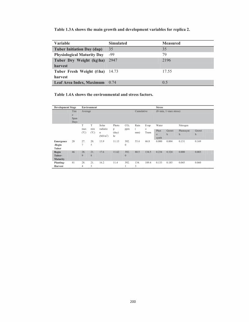
200
Table 1.3A shows the main growth and development variables for replica 2.
Variable Simulated Measured Tuber Initiation Day (dap) 35 35 Physiological Maturity Day -99 79 Tuber Dry Weight (kg\ha) harvest
2947 2196
Tuber Fresh Weight (t\ha) harvest
14.73 17.55
Leaf Area Index, Maximum 0.74 0.5 Table 1.4A shows the environmental and stress factors.
Development Stage Environment Stress Tim
e Span Days
Average Cumulative (0=min, 1=max stress)
T max (oC)
T min (oC)
Solar radiation (MJ/m2)
Photop (day) hr
CO2 ppm
Rain ( mm)
Evapo Trans
Water Nitrogen
Photo synth
Growth
Photosynth
Growth
Emergence-Begin Tuber
28 27.7
20.5
13.9 11.13 392.0
53.4 46.8 0.000 0.004 0.131 0.169
Begin Tuber-Maturity
46 28.9
21.8
17.6 11.62 392.0
80.5 134.5 0.234 0.324 0.000 0.003
Planting-Harvest
81 28.4
21.3
16.2 11.4 392.1
134.3
189.4 0.133 0.185 0.045 0.060

201
Appendix 2: Current climate simulations
Appendix 2 shows the soil chemical and physical properties for Banisogosogo soil,
Koronivia soil and Nacocolevu soil. It also provides the model output for current
climate simulation of these three areas using Desiree variety.
2.0A Current climate simulations
2.1.1A Soil profile information
2.1.1A Soil name: Koronivia Silt Loam
Profile name: KN30
Laboratory number: SB 9604A-E
Elevation (m): 19
Landform: Plateau surface, probably marine-planated
Relief: Flat
Parent material: In-situ rhyolitic outwash and tuffs
Vegetation: Para grass
Drainage: Moderately well drained
Classification: Humoxic Tropohumult, clayey, kaolintic, isohyperthermic
Soil classification:
Ap (0-18 cm): slightly moist, dark brown (10YR 3/3) silt loam, humic staining along
root channels, weakly developed fine and very fine nut with granular structure,
friable to firm, many fine roots, indistinct smooth boundary. Ochricepipedon.
Au (18-41 cm):slightly moist, olive brown (2.5 YR 4/4) and rubbed yellowish brown
(10YR 5/8) silt loam, common medium distinct yellowish red (5YR 4/6) mottles,
weakly developed very fine nut and granular structure, friable, common fine roots,
sharp wavy boundary.
Bt (41- 73): moist, yellowish brown (10YR 5/8) clay loam, few medium prominent
dark red (10Y 3/6) mottles, weakly developed coarse nut breaking to weak very fine
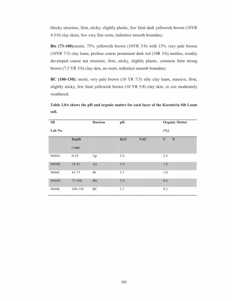
202
blocky structure, firm, sticky, slightly plastic, few faint dark yellowish brown (10YR
4.5/6) clay skins, few very fine roots, indistinct smooth boundary.
Bts (73-100):moist, 75% yellowish brown (10YR 5/8) with 15% very pale brown
(10YR 7/3) clay loam, profuse coarse prominent dark red (10R 3/6) mottles, weakly
developed coarse nut structure, firm, sticky, slightly plastic, common faint strong
brown (7.5 YR 5/6) clay skin, no roots, indistinct smooth boundary.
BC (100-130): moist, very pale brown (10 YR 7/3) silty clay loam, massive, firm,
slightly sticky, few faint yellowish brown (10 YR 5/8) clay skin, in situ moderately
weathered.
Table 2.0A shows the pH and organic matter for each layer of the Koronivia Silt Loam
soil.
SB
Lab No.
Horizon pH Organic Matter
(%)
Depth
( cm)
H2O NAF C N
9604A 0-18 Ap 5.4 2.6
9604B 18-41 Au 5.6 1.8
9604C 41-73 Bt 5.1 1.0
9604D 73-100 Bts 5.0 0.6
9604E 100-130 BC 5.1 0.3

203
Table 2.1A shows the chemical properties of the Koronivia Silt Loam soil.
SB
Lab No.
Horizon CEC (me./100g)
Cation Exchange KCL
Exch. acid
Depth
( cm)
BS (%)
Ca Mg K Na
9604A 0-18 Ap 10.6 6.4 60 5.0 1.00 0.16 0.24
9604B 18-41 Au 8.6 5.2 60 4.4 0.67 0.04 0.08
9604C 41-73 Bt 10.1 4.5 45 4.5 0.86 0.04 0.02
9604D 73-100
Bts 11.4 1.2 11 1.2 0.43 0.05 0.03
9604E 100-130
BC 13.9 1.1 8 1.1 0.34 0.09 0.15 18.2
Table 2.2A shows physical properties of the Koronivia Silt Loam soil.
SB
Lab No.
Horizon Particle size Fine to total clay ratio
15 bar water (%)
Clay (%)
Depth
( cm)
2.0-0.1 mm
2.0-0.2mm
0.2-0.02 mm
0.02-0.002 mm
<0.002 mm
<0.0002 mm
9604A 0-18 Ap 32 13 42 13 32 23 0.72 11.3 0.35
9604B 18-41 Au 29 8 41 10 41 32 0.78 13.4 0.33
9604C 41-73 Bt 13 3 19 9 69 56 0.81 27.4 0.40
9604D 73-100
Bts 6 2 12 10 76 51 0.67 29.1 0.38
9604E 100-130
BC 4 1 18 19 62 40 0.65 23.9 0.39

204
2.1.2A Soil map unit name: Nacocolevu soil, rolling phase
Area: 6 ha
Soil classification: OxicHalplustalf, fine, kaolinitic, isohyperthermic
Parent material: strongly weathered silicified marls and tuff
Geographical distribution: northern part of research station
Physiographical position and slope:rolling and easy rolling crests and ridges of
moderately dissected hill country. Slopes range form 7o-10o.
Vegetation and land use: cut-over bush, small area in Pinuscaribaea, some in
grasses
Elevation: 10-180 m
Annual rainfall: 1025-2973 mm
Soil profile description (Profile Sp 16 on 8o slope):
A (0-21 cm): dark reddish brown (5YR ¾ -3/3) silty clay loam, friable, sticky,
moderately plastic, moderately developed medium and fine nut structure, few fine
pores, many fine and medium rots, few medium (up to 3 cm diameter) strong brown
(7.5 YR 5/8) and yellowish red (5 YR 4/6) weakly weathered gravels coated with
dark reddish brown (5YR 3/3) humus, distinct smooth boundary.
Bt1 (21-40 cm): yellowish red (5YR 4/6) silty clay, friable, sticky, plastic,
moderately developed coarse and fine nut structure, many thin continuous reddish
brown (5 YR 4/4) clay coatings on peds, few dark reddish brown (5YR 3/2) humus
stains decreasing with depth, many fine pores, few fine and medium roots, distinct
smooth boundary.
Bt2 (40-72 cm): red (2.5 YR 4/6) silt loam, friable, slightly sticky, slightly plastic,
moderately developed fine blocky structure, many thin continuous (near red 2.5 YR
5/6) clay skin on peds, many fine distinct yellowish brown to strong brown (10YR-
7.5 YR 5/8) parent material remnants, few fine and medium roots, few fine roots,
distinct wavy boundary.

205
BCt (72-89 cm): red (2.5 YR 4/6) and strong brown (7.5 YR 5/8) silt loam to silt (
weathered parent rock), soft, nonsticky, nonplastic, massive to weakly developed
fine blocky structure, many veins and pockets of white (10 YR 8/2) parent material,
many thin discontinuous clay skins on peds, few fine roots, distinct irregular
boundary.
BC (89-125 cm): reddish brown (7.5 YR 6/6) silt, soft, massive breaking to weakly
developed platy structure, dark red (2.5 YR 3/6) clay coatings on peds, pockets of
white (10 YR 8/1) parent material.
Characteristics soil and site features: the red subsoils are the outstanding fine
characteristics of these soils. Profiles consists of dark reddish brown, friable silty
clay with moderately developed structure overlying yellowish red , friable silty clay
with moderately developed blocky structure and continuous clay skins on peds. This
rest on red, silt loam, friable with moderately developed blocky structure with
distinct clay skin on peds. Pockets of white parent material occur with increasing
depth. The soils occur on broad ridges and spurs mainly in the northern part of the
station.
Inclusion and variants within the map unit: pockets of Kabisi, rolling phase, may
occur (less than 10% of the map unit).
Associated soils: Barara soils on accumulation positions in the hill country. In places
the hill crest consist of Nacocolevu soils, rolling phase, but the associated hilly slope
consists of Kabisi soils, moderately steep to steep phase.
Drainage class: well drained
Erosion and Flooding: moderate soil creep
Chemical features: low base saturation, except directly above the lithic contact (at
146 cm depth in Profile Sp 16) where a medium base saturation was analyzed. Low
exchangeable magnesium and very low exchangeable calcium and potassium.
Medium values of exchangeable sodium. Organic carbon is low.
Soil limitation and potential: low natural nutrient levels. Erosion risk under
intensive uses. Pastoral uses (beef, sheep).

206
Table 2.3A shows the Nacocolevu Rolling Phase soil properties.
Soil and
sample
number
Horiz Organic Cation Exchange
Nacocolevu
soil, rolling
phase
KRS T
1838-43
Depth
( cm)
Silt Clay Carbon
(%)
CEC
(me%)
TEB
(me%)
BS
(%)
Ca
(me%)
Mg
(me%)
K
(me%)
Na(me%)
0-21 A 26 60 3.37 16.0 4.4 28 1.9 1.8 0.2 0.5
21-40 Bt1 25 70 2.18 13.1 2.1 16 0.9 0.7 0.1 0.5
40-72 Bt2 34 64 0.89 13.0 1.9 15 0.8 0.5 0.1 0.5
72-89 BCt 38 53 0.58 13.3 1.9 100 0.7 0.5 0.1 0.5
89-
125
BC 55 41 0.48 12.3 2.2 18 0.9 0.7 0.1 0.6
136-
146
BC N.D 20.2 11.1 55 9.7 0.8 0.1 0.5
Table 2.4A shows the information on weather station and soil for each location.
Location Experiment Number
Weather Station Soil
Koronivia CCRA1250 Non-Potential
FJNU Koronivia Silt Loam
CCRA1255 Potential FJNU Koronivia Silt Loam
Nacocolevu CCRA1260 Non-Potential
FJNC Nacocolevu Soil, Rolling Phase
CCRA1265 Potential FJNC Nacocolevu Soil, Rolling Phase

207
Table 2.5A shows the potential simulated crop and soil status at main development
stages for Banisogosogo.
Date Crop
Age Growth Stage
Biomass
(kg\ha)
LAI Leaf Number
Crop (kg\ha)
%N Water Stress
Nitrogen Stress
P1 Stress
P2 Stress
RSTG
1 Jun
0 Start Sim 0 0 0 0 0 0 0 0 0 0
2 Jul
0 Sowing 0 0 0 0 0 0 0 0 0 0
9 Jul
7 Emergence 0 0 0 0 0 0 0 0 0 0
9 Aug
35 Beg Tuber Initiation
0 0 0 0 0 0 0 0 0 0
20 Sep
80 Harvest 0 0 0 0 0 0 0 0 0 0
Table 2.6A shows the environmental and stress factors.
Development Stage Environment Stress
Time Span Days
Average Cumulative (0=min, 1=max stress)
T max (oC)
T min (oC)
Solar radiation (MJ/m2)
Photop (day) hr
CO2 ppm
Rain ( mm)
Evapo Trans
Water Nitrogen
Photo synth
Growth
Photosynth
Growth
Emergence-Begin Tuber
31 27.8
20.5
20.7 11.14 392.0
69.4 46.8 0.000 0.000 0.000 0.000
Begin Tuber-Maturity
43 28.9
21.8
21.7 11.65 392.0
64.5 134.5 0.000 0.000 0.000 0.000
Planting-Harvest
81 28.4
21.3
16.2 11.4 392.1
134.3
189.4 0.000 0.000 0.000 0.000

208
Table 2.7A shows the non-potential simulated crop and soil status at main development
stages for Banisogosogo.
Date Crop
Age Growth Stage
Biomass
(kg\ha)
LAI Leaf Number
Crop (kg\ha)
%N Water Stress
Nitrogen Stress
P1 Stress
P2 Stress
RSTG
1 Jun
0 Start Sim 0 0 0 0 0 0 0 0 0 5
2 Jul
0 Sowing 0 0 0 0 0 0 0 0 0 7
6 Jul
7 Emergence 0 0.01 0 5 42.8 0 0 0 0 1
9 Aug
35 Beg Tuber Initiation
0 0.67 0 194 43.9 0 0.16 0 0 2
20 Sep
80 Harvest 0 1.60 0 1162 19.7 0.33 0.03 0 0 2
Table 2.8A shows the environmental and stress factors for Banisogosogo.
Development Stage Environment Stress
Time Span Days
Average Cumulative (0=min, 1=max stress)
T max (oC)
T min (oC)
Solar radiation (MJ/m2)
Photop (day) hr
CO2 ppm
Rain ( mm)
Evapo Trans
Water Nitrogen
Photo synth
Growth
Photosynth
Growth
Emergence-Begin Tuber
28 27.7
20.5
13.9 11.13 392.0
53.4 49.3 0.000 0.004 0.120 0.159
Begin Tuber-Maturity
46 28.9
21.8
17.6 11.62 392.0
80.5 160.3 0.240 0.324 0.004 0.029
Planting-Harvest
81 28.4
21.3
16.2 11.4 392.1
134.3
217.7 0.136 0.184 0.044 0.071
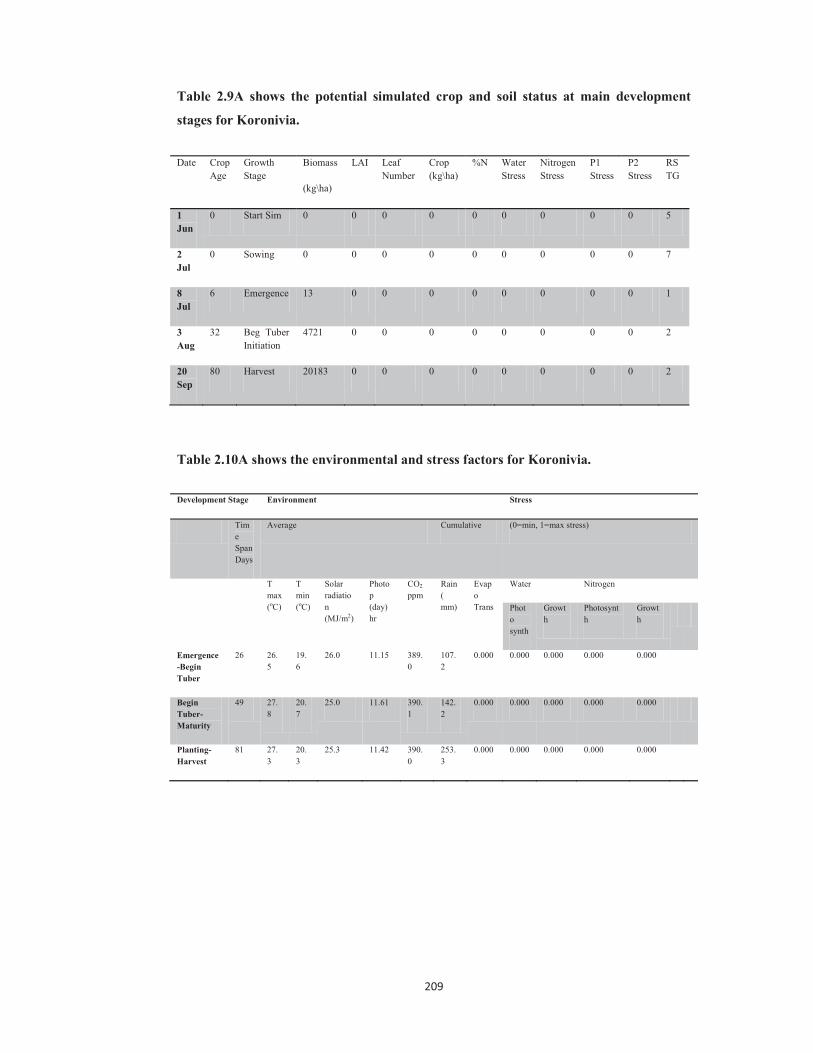
209
Table 2.9A shows the potential simulated crop and soil status at main development
stages for Koronivia.
Date Crop
Age Growth Stage
Biomass
(kg\ha)
LAI Leaf Number
Crop (kg\ha)
%N Water Stress
Nitrogen Stress
P1 Stress
P2 Stress
RSTG
1 Jun
0 Start Sim 0 0 0 0 0 0 0 0 0 5
2 Jul
0 Sowing 0 0 0 0 0 0 0 0 0 7
8 Jul
6 Emergence 13 0 0 0 0 0 0 0 0 1
3 Aug
32 Beg Tuber Initiation
4721 0 0 0 0 0 0 0 0 2
20 Sep
80 Harvest 20183 0 0 0 0 0 0 0 0 2
Table 2.10A shows the environmental and stress factors for Koronivia.
Development Stage Environment Stress
Time Span Days
Average Cumulative (0=min, 1=max stress)
T max (oC)
T min (oC)
Solar radiation (MJ/m2)
Photop (day) hr
CO2 ppm
Rain ( mm)
Evapo Trans
Water Nitrogen
Photo synth
Growth
Photosynth
Growth
Emergence-Begin Tuber
26 26.5
19.6
26.0 11.15 389.0
107.2
0.000 0.000 0.000 0.000 0.000
Begin Tuber-Maturity
49 27.8
20.7
25.0 11.61 390.1
142.2
0.000 0.000 0.000 0.000 0.000
Planting-Harvest
81 27.3
20.3
25.3 11.42 390.0
253.3
0.000 0.000 0.000 0.000 0.000

210
Table 2.11A shows the non-potential simulated crop and soil status at main
development stages for Koronivia.
Date Crop
Age Growth Stage
Biomass
(kg\ha)
LAI Leaf Number
Crop (kg\ha)
%N Water Stress
Nitrogen Stress
P1 Stress
P2 Stress
RSTG
1 Jun
0 Start Sim 0 0 0 0 0 0 0 0 0 5
2 Jul
0 Sowing 0 0 0 0 0 0 0 0 0 7
8 Jul
6 Emergence 11 0.01 0 5 42.9 0 0 0 0 1
1 Aug
30 Beg Tuber Initiation
768 1.17 0 286 37.3 0.22 0.15 0 0 2
20 Sep
80 Harvest 6459 1.93 0 1384 21.4 0.47 0.12 0 0 2
Table 2.12A shows the environmental and stress factors for Koronivia.
Development Stage Environment Stress
Time Span Days
Average Cumulative (0=min, 1=max stress)
T max (oC)
T min (oC)
Solar radiation (MJ/m2)
Photop (day) hr
CO2 ppm
Rain ( mm)
Evapo Trans
Water Nitrogen
Photo synth
Growth
Photosynth
Growth
Emergence-Begin Tuber
24 26.5
19.4
26.1 11.14 389.9
94.2 83.3 0.119 0.219 0.100 0.139
Begin Tuber-Maturity
51 27.8
20.8
25.0 11.59 390.1
155.2
194.0 0.426 0.464 0.080 0.124
Planting-Harvest
81 27.3
20.3
25.3 11.42 390.0
253.3
301.1 0.304 0.357 0.080 0.119
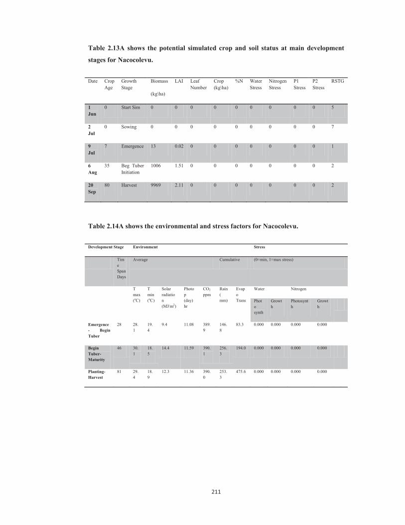
211
Table 2.13A shows the potential simulated crop and soil status at main development
stages for Nacocolevu.
Date Crop
Age Growth Stage
Biomass
(kg\ha)
LAI Leaf Number
Crop (kg\ha)
%N Water Stress
Nitrogen Stress
P1 Stress
P2 Stress
RSTG
1 Jun
0 Start Sim 0 0 0 0 0 0 0 0 0 5
2 Jul
0 Sowing 0 0 0 0 0 0 0 0 0 7
9 Jul
7 Emergence 13 0.02 0 0 0 0 0 0 0 1
6 Aug
35 Beg Tuber Initiation
1006 1.51 0 0 0 0 0 0 0 2
20 Sep
80 Harvest 9969 2.11 0 0 0 0 0 0 0 2
Table 2.14A shows the environmental and stress factors for Nacocolevu.
Development Stage Environment Stress
Time Span Days
Average Cumulative (0=min, 1=max stress)
T max (oC)
T min (oC)
Solar radiation (MJ/m2)
Photop (day) hr
CO2 ppm
Rain ( mm)
Evapo Trans
Water Nitrogen
Photo synth
Growth
Photosynth
Growth
Emergence- Begin Tuber
28 28.1
19.4
9.4 11.08 389.9
146.8
83.3 0.000 0.000 0.000 0.000
Begin Tuber-Maturity
46 30.1
18.5
14.4 11.59 390.1
256.3
194.0 0.000 0.000 0.000 0.000
Planting-Harvest
81 29.4
18.9
12.3 11.36 390.0
253.3
475.6 0.000 0.000 0.000 0.000

212
Table 2.15A shows the non-potential simulated crop and soil status at main
development stages for Nacocolevu.
Date Crop
Age Growth Stage
Biomass
(kg\ha)
LAI Leaf Number
Crop (kg\ha)
%N Water Stress
Nitrogen Stress
P1 Stress
P2 Stress
RSTG
1 Jun
0 Start Sim 0 0 0 0 0 0 0 0 0 5
2 Jul
0 Sowing 0 0 0 0 0 0 0 0 0 7
9 Jul
7 Emergence 11 0.01 0 5 42.9 0 0 0 0 1
4 Aug
33 Beg Tuber Initiation
481 0.73 0 238 49.6 0 0.07 0 0 2
20 Sep
80 Harvest 5984 0.77 0 1112 18.6 0 0 0 0 2
Table 2.16A shows the environmental and stress factors for Nacocolevu.
Development Stage Environment Stress
Time Span Days
Average Cumulative (0=min, 1=max stress)
T max (oC)
T min (oC)
Solar radiation (MJ/m2)
Photop (day) hr
CO2 ppm
Rain ( mm)
Evapo Trans
Water Nitrogen
Photo synth
Growth
Photosynth
Growth
Emergence- Begin Tuber
26 28.1
19.3
9.1 11.07 389.9
138.7
63.7 0.000 0.000 0.046 0.074
Begin Tuber-Maturity
48 30.1
18.6
14.3 11.57 390.1
264.4
172.4 0.000 0.000 0.000 0.000
Planting-Harvest
81 29.4
18.9
12.3 11.36 390.0
475.6
253.7 0.000 0.000 0.015 0.024

213
Appendix 3: Future climate simulations
Appendix 3 provides the model output for potential and non-potential future climate
simulations. The model simulation was conducted for Banisogosogo, Koronivia and
Nacocolevu using Desiree. PCCSP A1B and A2 emission scenarios were used.
Likewise, it also shows the optimisation results for planting date, row spacing,
fertiliser application, irrigation application and planting depth.
3.0A Future climate simulation
3.1A Results
3.1.1A Banisogosogo climate simulation
Table 3.0A shows the potential simulated crop and soil status at main development
stages for 2030 Medium emission scenario.
Date Crop
Age Growth Stage
Biomass
(kg\ha)
LAI Leaf Number
Crop (kg\ha)
%N Water Stress
Nitrogen Stress
P1 Stress
P2 Stress
RSTG
1 Jun
0 Start Sim 0 0 0 0 0 0 0 0 0 5
2 Jul
0 Sowing 0 0 0 0 0 0 0 0 0 7
10 Jul
8 Emergence 12 0.02 0 0 0 0 0 0 0 1
28 Aug
57 Beg Tuber Initiation
7129 10.54 0 0 0 0 0 0 0 2
20 Sep
80 Harvest 9955 8.44 0 0 0 0 0 0 0 2
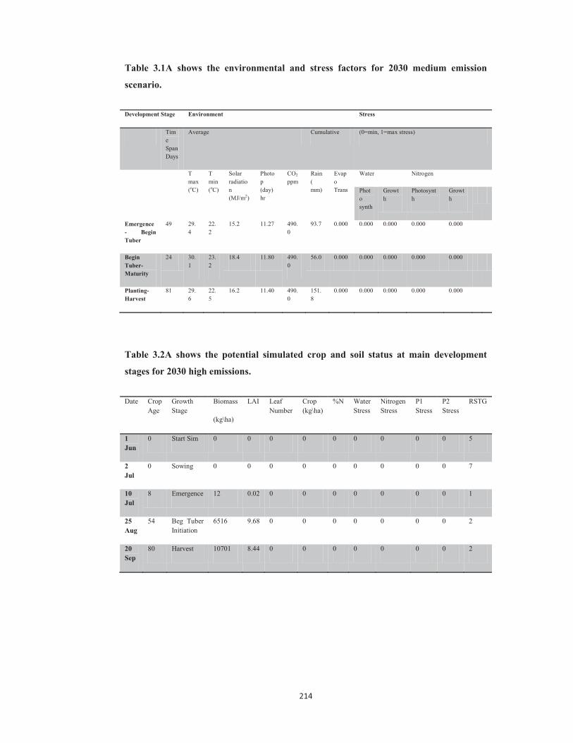
214
Table 3.1A shows the environmental and stress factors for 2030 medium emission
scenario.
Development Stage Environment Stress
Time Span Days
Average Cumulative (0=min, 1=max stress)
T max (oC)
T min (oC)
Solar radiation (MJ/m2)
Photop (day) hr
CO2 ppm
Rain ( mm)
Evapo Trans
Water Nitrogen
Photo synth
Growth
Photosynth
Growth
Emergence- Begin Tuber
49 29.4
22.2
15.2 11.27 490.0
93.7 0.000 0.000 0.000 0.000 0.000
Begin Tuber-Maturity
24 30.1
23.2
18.4 11.80 490.0
56.0 0.000 0.000 0.000 0.000 0.000
Planting-Harvest
81 29.6
22.5
16.2 11.40 490.0
151.8
0.000 0.000 0.000 0.000 0.000
Table 3.2A shows the potential simulated crop and soil status at main development
stages for 2030 high emissions.
Date Crop
Age Growth Stage
Biomass
(kg\ha)
LAI Leaf Number
Crop (kg\ha)
%N Water Stress
Nitrogen Stress
P1 Stress
P2 Stress
RSTG
1 Jun
0 Start Sim 0 0 0 0 0 0 0 0 0 5
2 Jul
0 Sowing 0 0 0 0 0 0 0 0 0 7
10 Jul
8 Emergence 12 0.02 0 0 0 0 0 0 0 1
25 Aug
54 Beg Tuber Initiation
6516 9.68 0 0 0 0 0 0 0 2
20 Sep
80 Harvest 10701 8.44 0 0 0 0 0 0 0 2

215
Table 3.3A shows the environmental and stress factors.
Development Stage Environment Stress
Time Span Days
Average Cumulative (0=min, 1=max stress)
T max (oC)
T min (oC)
Solar radiation (MJ/m2)
Photop (day) hr
CO2 ppm
Rain ( mm)
Evapo Trans
Water Nitrogen
Photo synth
Growth
Photosynth
Growth
Emergence- Begin Tuber
46 29.3
22.0
14.9 11.25 520.0
95.3 0.000 0.000 0.000 0.000 0.000
Begin Tuber-Maturity
27 29.8
22.8
18.6 11.77 520.0
57.0 0.000 0.000 0.000 0.000 0.000
Planting-Harvest
81 29.4
22.2
16.2 11.40 520.0
154.4
0.000 0.000 0.000 0.000 0.000
3.1.2A Banisogosogo non-potential simulation
Table 3.4A shows the non-potential simulated crop and soil status at main development
stages for 2030 medium emissions.
Date Crop
Age Growth Stage
Biomass
(kg\ha)
LAI Leaf Number
Crop (kg\ha)
%N Water Stress
Nitrogen Stress
P1 Stress
P2 Stress
RSTG
1 Jun
0 Start Sim 0 0 0 0 0 0 0 0 0 5
2 Jul
0 Sowing 0 0 0 0 0 0 0 0 0 7
11 Jul
9 Emergence 10 0.01 0 4 42.8 0 0 0 0 1
26 Aug
55 Beg Tuber Initiation
3397 5.15 0 1272 37.4 0 0.10 0 0 2
20 Sep
80 Harvest 6214 6.68 0 1825 29.4 0.20 0.28 0 0 2

216
Table 3.5A shows the environmental and stress factors. Development Stage Environment Stress
Time Span Days
Average Cumulative (0=min, 1=max stress)
T max (oC)
T min (oC)
Solar radiation (MJ/m2)
Photop (day) hr
CO2 ppm
Rain ( mm)
Evapo Trans
Water Nitrogen
Photo synth
Growth
Photosynth
Growth
Emergence- Begin Tuber
46 29.5
22.2
15.0 11.26 490.0
93.7 130.6 0.000 0.000 0.069 0.099
Begin Tuber-Maturity
26 30.0
23.1
18.6 11.78 490.0
56.0 106.5 0.081 0.188 0.234 0.272
Planting-Harvest
81 29.6
22.5
16.2 11.40 490.0
151.8
247.6 0.026 0.060 0.114 0.144
Table 3.6A shows the non-potential simulated crop and soil status at main development
stages for 2030 high emissions.
Date Crop
Age Growth Stage
Biomass
(kg\ha)
LAI Leaf Number
Crop (kg\ha)
%N Water Stress
Nitrogen Stress
P1 Stress
P2 Stress
RSTG
1 Jun
0 Start Sim 0 0 0 0 0 0 0 0 0 5
2 Jul
0 Sowing 0 0 0 0 0 0 0 0 0 7
10 Jul
8 Emergence 10 0.01 0 4 0 0 0 0 0 1
22 Aug
51 Beg Tuber Initiation
3093 4.71 0 1251 0 0 0.10 0 0 2
20 Sep
80 Harvest 6928 6.82 0 1898 0 0.14 0.27 0 0 2

217
Table 3.7A shows the environmental and stress factors.
Development Stage Environment Stress
Time Span Days
Average Cumulative (0=min, 1=max stress)
T max (oC)
T min (oC)
Solar radiation (MJ/m2)
Photop (day) hr
CO2 ppm
Rain ( mm)
Evapo Trans
Water Nitrogen
Photo synth
Growth
Photosynth
Growth
Emergence- Begin Tuber
43 29.2
22.0
14.7 11.23 520.0
95.3 114.9 0.000 0.000 0.074 0.100
Begin Tuber-Maturity
30 29.8
22.7
18.5 11.75 520.0
57.0 126.1 0.044 0.135 0.223 0.262
Planting-Harvest
81 29.4
22.3
16.2 11.40 520.0
154.4
250.7 0.016 0.050 0.122 0.150
Table 3.8A shows the non-potential simulated crop and soil status at main development
stages for 2055 medium emission.
Date Crop
Age Growth Stage
Biomass
(kg\ha)
LAI Leaf Number
Crop (kg\ha)
%N Water Stress
Nitrogen Stress
P1 Stress
P2 Stress
RSTG
1 Jun
0 Start Sim 0 0 0 0 0 0 0 0 0 5
2 Jul
0 Sowing 0 0 0 0 0 0 0 0 0 7
12 Jul
10 Emergence 10 0.01 0 4 42.8 0 0 0 0 1
12 Sep
72 Beg Tuber Initiation
4333 7.87 0 1696 31.8 0.07 0.17 0 0 2
20 Sep
80 Harvest 5487 7.25 0 1808 33.0 0.18 0.38 0 0 2
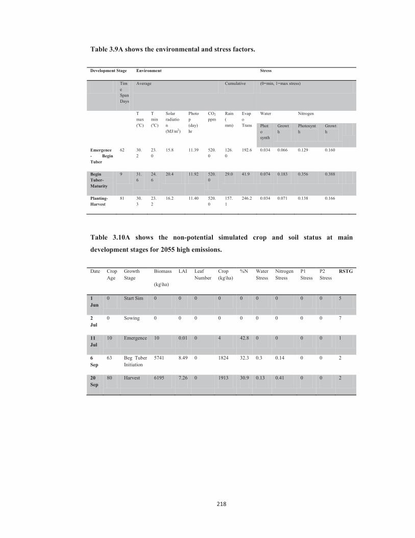
218
Table 3.9A shows the environmental and stress factors.
Development Stage Environment Stress
Time Span Days
Average Cumulative (0=min, 1=max stress)
T max (oC)
T min (oC)
Solar radiation (MJ/m2)
Photop (day) hr
CO2 ppm
Rain ( mm)
Evapo Trans
Water Nitrogen
Photo synth
Growth
Photosynth
Growth
Emergence- Begin Tuber
62 30.2
23.0
15.8 11.39 520.0
126.0
192.6 0.034 0.066 0.129 0.160
Begin Tuber-Maturity
9 31.6
24.6
20.4 11.92 520.0
29.0 41.9 0.074 0.183 0.356 0.388
Planting-Harvest
81 30.3
23.2
16.2 11.40 520.0
157.1
246.2 0.034 0.071 0.138 0.166
Table 3.10A shows the non-potential simulated crop and soil status at main
development stages for 2055 high emissions.
Date Crop
Age Growth Stage
Biomass
(kg\ha)
LAI Leaf Number
Crop (kg\ha)
%N Water Stress
Nitrogen Stress
P1 Stress
P2 Stress
RSTG
1 Jun
0 Start Sim 0 0 0 0 0 0 0 0 0 5
2 Jul
0 Sowing 0 0 0 0 0 0 0 0 0 7
11 Jul
10 Emergence 10 0.01 0 4 42.8 0 0 0 0 1
6 Sep
63 Beg Tuber Initiation
5741 8.49 0 1824 32.3 0.3 0.14 0 0 2
20 Sep
80 Harvest 6195 7.26 0 1913 30.9 0.13 0.41 0 0 2

219
Table 3.11A shows the environmental and stress factors.
Development Stage Environment Stress
Time Span Days
Average Cumulative (0=min, 1=max stress)
T max (oC)
T min (oC)
Solar radiation (MJ/m2)
Photop (day) hr
CO2 ppm
Rain ( mm)
Evapo Trans
Water Nitrogen
Photo synth
Growth
Photosynth
Growth
Emergence- Begin Tuber
57 30.0
22.8
15.5 11.34 992.1
125.3
167.7 0.011 0.031 0.121 0.156
Begin Tuber-Maturity
15 30.7
23.6
19.4 11.87 992.0
29.7 69.3 0.034 0.125 0.377 0.408
Planting-Harvest
81 30.1
23 16.2 11.40 992.0
157.1
247.7 0.014 0.034 0.155 0.185
3.1.3A Koronivia potential simulation
Table 3.12A shows the potential simulated crop and soil status at main development
stages for 2030 medium emissions.
Date Crop
Age Growth Stage
Biomass
(kg\ha)
LAI Leaf Number
Crop (kg\ha)
%N Water Stress
Nitrogen Stress
P1 Stress
P2 Stress
RSTG
1 Jun
0 Start Sim 0 0 0 0 0 0 0 0 0 5
2 Jul
0 Sowing 0 0 0 0 0 0 0 0 0 7
9 Jul
7 Emergence 12 0.02 0 0 0 0 0 0 0 1
13 Aug
42 Beg Tuber Initiation
8200 12.12 0 0 0 0 0 0 0 2
20 Sep
80 Harvest 16385 8.61 0 0 0 0 0 0 0 5

220
Table 3.13A shows the environmental and stress factors.
Development Stage Environment Stress
Time Span Days
Average Cumulative (0=min, 1=max stress)
T max (oC)
T min (oC)
Solar radiation (MJ/m2)
Photop (day) hr
CO2 ppm
Rain ( mm)
Evapo Trans
Water Nitrogen
Photo synth
Growth
Photosynth
Growth
Emergence- Begin Tuber
35 28.0
21.0
26 11.2 490.0
140.7
0.000 0.000 0.000 0.000 0.000
Begin Tuber-Maturity
39 29.1
22.0
24.8 11.68 490.0
141.1
0.000 0.000 0.000 0.000 0.000
Planting-Harvest
81 28.5
21.5
25.3 11.42 490.0
286.2
0.000 0.000 0.000 0.000 0.000
Table 3.14A shows the potential simulated crop and soil status at main development
stages for 2030 high emissions.
Date Crop
Age Growth Stage
Biomass
(kg\ha)
LAI Leaf Number
Crop (kg\ha)
%N Water Stress
Nitrogen Stress
P1 Stress
P2 Stress
RSTG
1 Jun
0 Start Sim 0 0 0 0 0 0 0 0 0 5
2 Jul
0 Sowing 0 0 0 0 0 0 0 0 0 7
9 Jul
7 Emergence 12 0.02 0 0 0 0 0 0 0 1
11 Aug
40 Beg Tuber Initiation
7807 11.59 0 0 0 0 0 0 0 2
20 Sep
80 Harvest 17503 8.66 0 0 0 0 0 0 0 5
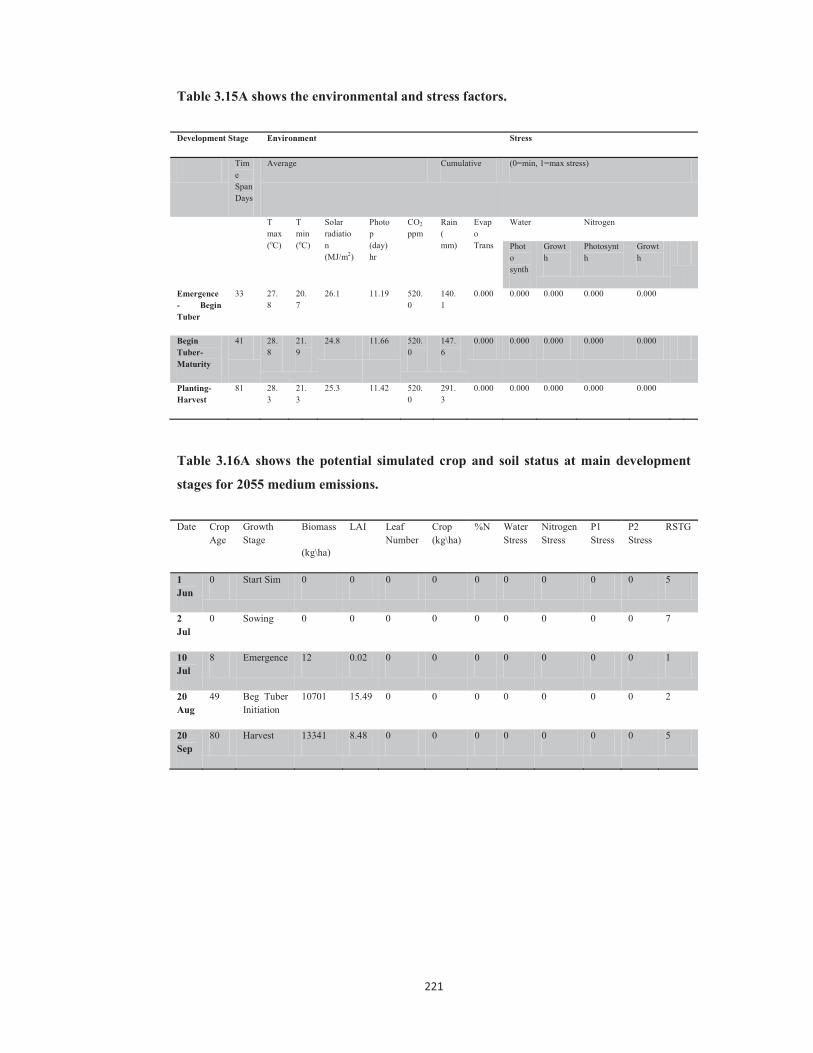
221
Table 3.15A shows the environmental and stress factors.
Development Stage Environment Stress
Time Span Days
Average Cumulative (0=min, 1=max stress)
T max (oC)
T min (oC)
Solar radiation (MJ/m2)
Photop (day) hr
CO2 ppm
Rain ( mm)
Evapo Trans
Water Nitrogen
Photo synth
Growth
Photosynth
Growth
Emergence- Begin Tuber
33 27.8
20.7
26.1 11.19 520.0
140.1
0.000 0.000 0.000 0.000 0.000
Begin Tuber-Maturity
41 28.8
21.9
24.8 11.66 520.0
147.6
0.000 0.000 0.000 0.000 0.000
Planting-Harvest
81 28.3
21.3
25.3 11.42 520.0
291.3
0.000 0.000 0.000 0.000 0.000
Table 3.16A shows the potential simulated crop and soil status at main development
stages for 2055 medium emissions.
Date Crop
Age Growth Stage
Biomass
(kg\ha)
LAI Leaf Number
Crop (kg\ha)
%N Water Stress
Nitrogen Stress
P1 Stress
P2 Stress
RSTG
1 Jun
0 Start Sim 0 0 0 0 0 0 0 0 0 5
2 Jul
0 Sowing 0 0 0 0 0 0 0 0 0 7
10 Jul
8 Emergence 12 0.02 0 0 0 0 0 0 0 1
20 Aug
49 Beg Tuber Initiation
10701 15.49 0 0 0 0 0 0 0 2
20 Sep
80 Harvest 13341 8.48 0 0 0 0 0 0 0 5

222
Table 3.17A shows the environmental and stress factors.
Development Stage Environment Stress
Time Span Days
Average Cumulative (0=min, 1=max stress)
T max (oC)
T min (oC)
Solar radiation (MJ/m2)
Photop (day) hr
CO2 ppm
Rain ( mm)
Evapo Trans
Water Nitrogen
Photo synth
Growth
Photosynth
Growth
Emergence- Begin Tuber
41 28.9
21.7
25.8 11.25 520.0
145.7
0.000 0.000 0.000 0.000 0.000
Begin Tuber-Maturity
32 29.8
23.0
24.8 11.73 520.0
146.1
0.000 0.000 0.000 0.000 0.000
Planting-Harvest
81 29.2
22.2
25.3 11.42 520.0
296.4
0.000 0.000 0.000 0.000 0.000
Table 3.18A shows the potential simulated crop and soil status at main development
stages for 2055 high emissions.
Date Crop
Age Growth Stage
Biomass
(kg\ha)
LAI Leaf Number
Crop (kg\ha)
%N Water Stress
Nitrogen Stress
P1 Stress
P2 Stress
RSTG
1 Jun
0 Start Sim 0 0 0 0 0 0 0 0 0 5
2 Jul
0 Sowing 0 0 0 0 0 0 0 0 0 7
10 Jul
8 Emergence 12 0.02 0 0 0 0 0 0 0 1
18 Aug
47 Beg Tuber Initiation
12533 17.92 0 0 0 0 0 0 0 2
20 Sep
80 Harvest 16209 8.54 0 0 0 0 0 0 0 5

223
Table 3.19A shows the environmental and stress factors.
Development Stage Environment Stress
Time Span Days
Average Cumulative (0=min, 1=max stress)
T max (oC)
T min (oC)
Solar radiation (MJ/m2)
Photop (day) hr
CO2 ppm
Rain ( mm)
Evapo Trans
Water Nitrogen
Photo synth
Growth
Photosynth
Growth
Emergence- Begin Tuber
39 28.6
21.6
25.8 11.24 990.0
145.7
0.000 0.000 0.000 0.000 0.000
Begin Tuber-Maturity
34 29.6
22.6
24.9 11.72 990.2
146.1
0.000 0.000 0.000 0.000 0.000
Planting-Harvest
81 29.0
22 25.3 11.42 990.0
296.4
0.000 0.000 0.000 0.000 0.000
3.1.4A Koronivia non-potential yield
Table 3.20A shows the non-potential simulated crop and soil status at main
development stages for 2030 medium emissions.
Date Crop
Age Growth Stage
Biomass
(kg\ha)
LAI Leaf Number
Crop (kg\ha)
%N Water Stress
Nitrogen Stress
P1 Stress
P2 Stress
RSTG
1 Jun
0 Start Sim 0 0 0 0 0 0 0 0 0 5
2 Jul
0 Sowing 0 0 0 0 0 0 0 0 0 7
9 Jul
7 Emergence 11 0.01 0 5 42.8 0 0 0 0 1
8 Aug
37 Beg Tuber Initiation
2311 3.54 0 929 40.2 0.13 0.11 0 0 2
20 Sep
80 Harvest 5501 3.23 0 1409 25.6 0.43 0.10 0 0 5

224
Table 3.21A shows the environmental and stress factors.
Development Stage Environment Stress
Time Span Days
Average Cumulative (0=min, 1=max stress)
T max (oC)
T min (oC)
Solar radiation (MJ/m2)
Photop (day) hr
CO2 ppm
Rain ( mm)
Evapo Trans
Water Nitrogen
Photo synth
Growth
Photosynth
Growth
Emergence- Begin Tuber
30 27.8
20.8
26.1 11.18 490.0
136.3
125.7 0.070 0.134 0.073 0.113
Begin Tuber-Maturity
44 29.1
22.0
24.9 11.64 490.2
145.5
174.6 0.376 0.421 0.052 0.099
Planting-Harvest
81 28.5
21.5
25.3 11.42 490.0
286.2
326.1 0.230 0.278 0.055 0.096
Table 3.22A shows the non-potential simulated crop and soil status at main
development stages for 2030 high emissions.
Date Crop
Age Growth Stage
Biomass
(kg\ha)
LAI Leaf Number
Crop (kg\ha)
%N Water Stress
Nitrogen Stress
P1 Stress
P2 Stress
RSTG
1 Jun
0 Start Sim 0 0 0 0 0 0 0 0 0 5
2 Jul
0 Sowing 0 0 0 0 0 0 0 0 0 7
9 Jul
7 Emergence 11 0.01 0 5 42.8 0 0 0 0 1
9 Aug
36 Beg Tuber Initiation
2263 3.46 0 922 40.7 0.14 0.12 0 0 2
20 Sep
811 Harvest 5777 3.1 0 1406 24.3 0.41 0.12 0 0 5
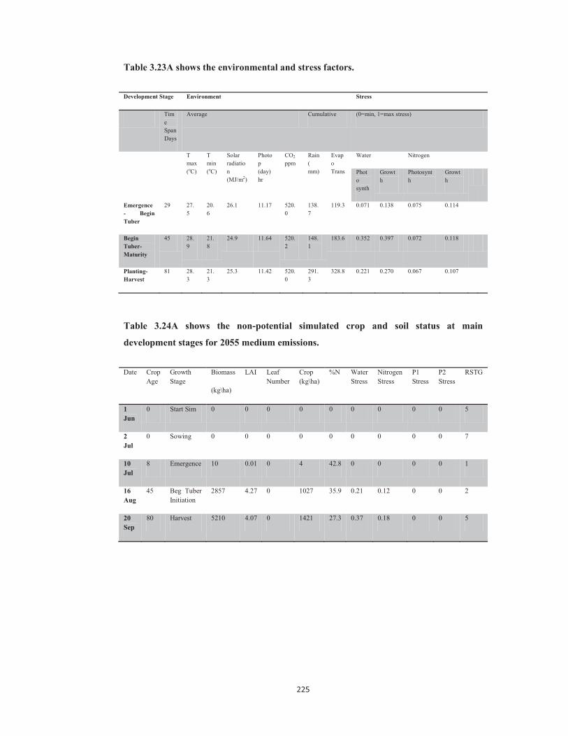
225
Table 3.23A shows the environmental and stress factors.
Development Stage Environment Stress
Time Span Days
Average Cumulative (0=min, 1=max stress)
T max (oC)
T min (oC)
Solar radiation (MJ/m2)
Photop (day) hr
CO2 ppm
Rain ( mm)
Evapo Trans
Water Nitrogen
Photo synth
Growth
Photosynth
Growth
Emergence- Begin Tuber
29 27.5
20.6
26.1 11.17 520.0
138.7
119.3 0.071 0.138 0.075 0.114
Begin Tuber-Maturity
45 28.9
21.8
24.9 11.64 520.2
148.1
183.6 0.352 0.397 0.072 0.118
Planting-Harvest
81 28.3
21.3
25.3 11.42 520.0
291.3
328.8 0.221 0.270 0.067 0.107
Table 3.24A shows the non-potential simulated crop and soil status at main
development stages for 2055 medium emissions.
Date Crop
Age Growth Stage
Biomass
(kg\ha)
LAI Leaf Number
Crop (kg\ha)
%N Water Stress
Nitrogen Stress
P1 Stress
P2 Stress
RSTG
1 Jun
0 Start Sim 0 0 0 0 0 0 0 0 0 5
2 Jul
0 Sowing 0 0 0 0 0 0 0 0 0 7
10 Jul
8 Emergence 10 0.01 0 4 42.8 0 0 0 0 1
16 Aug
45 Beg Tuber Initiation
2857 4.27 0 1027 35.9 0.21 0.12 0 0 2
20 Sep
80 Harvest 5210 4.07 0 1421 27.3 0.37 0.18 0 0 5

226
Table 3.25A shows the environmental and stress factors.
Development Stage Environment Stress
Time Span Days
Average Cumulative (0=min, 1=max stress)
T max (oC)
T min (oC)
Solar radiation (MJ/m2)
Photop (day) hr
CO2 ppm
Rain ( mm)
Evapo Trans
Water Nitrogen
Photo synth
Growth
Photosynth
Growth
Emergence- Begin Tuber
37 28.7
21.9
25.7 11.23 550.0
145.7
155.9 0.124 0.185 0.075 0.116
Begin Tuber-Maturity
36 29.9
22.7
25.0 11.70 550.2
146.1
147.7 0.351 0.384 0.137 0.180
Planting-Harvest
81 29.2
22.2
25.3 11.42 550.0
296.4
330.9 0.212 0.255 0.095 0.133
Table 3.26A shows the non-potential simulated crop and soil status at main
development stages for 2055 high emissions.
Date Crop
Age Growth Stage
Biomass
(kg\ha)
LAI Leaf Number
Crop (kg\ha)
%N Water Stress
Nitrogen Stress
P1 Stress
P2 Stress
RSTG
1 Jun
0 Start Sim 0 0 0 0 0 0 0 0 0 5
2 Jul
0 Sowing 0 0 0 0 0 0 0 0 0 7
10 Jul
8 Emergence 10 0.01 0 4 42.8 0 0 0 0 1
14 Aug
43 Beg Tuber Initiation
3122 4.68 0 1096 35.1 0.15 0.15 0 0 2
20 Sep
80 Harvest 5668 3.56 0 1406 24.8 0.37 0.22 0 0 5

227
Table 3.27A shows the environmental and stress factors.
Development Stage Environment Stress
Time Span Days
Average Cumulative (0=min, 1=max stress)
T max (oC)
T min (oC)
Solar radiation (MJ/m2)
Photop (day) hr
CO2 ppm
Rain ( mm)
Evapo Trans
Water Nitrogen
Photo synth
Growth
Photosynth
Growth
Emergence- Begin Tuber
35 28.5
21.6
25.9 11.21 989.9
145.7
151.6 0.068 0.131 0.104 0.143
Begin Tuber-Maturity
38 29.6
22.5
24.9 11.69 990.9
146.1
151.6 0.356 0.385 0.179 0.120
Planting-Harvest
81 29.0
22.0
25.3 11.42 990.0
296.4
330.6 0.197 0.237 0.129 0.165
Table 3.28A shows the non-potential simulated crop and soil status at main
development stages for 2090 medium emissions.
Date Crop
Age Growth Stage
Biomass
(kg\ha)
LAI Leaf Number
Crop (kg\ha)
%N Water Stress
Nitrogen Stress
P1 Stress
P2 Stress
RSTG
1 Jun
0 Start Sim 0 0 0 0 0 0 0 0 0 5
2 Jul
0 Sowing 0 0 0 0 0 0 0 0 0 7
12 Jul
10 Emergence 11 0.01 0 5 42.9 0 0 0 0 1
25 Aug
54 Beg Tuber Initiation
3327 4.93 0 1110 33.4 0.33 0.16 0 0 2
20 Sep
80 Harvest 4894 5.16 0 1416 28.9 0.24 0.33 0 0 5

228
Table 3.29A shows the environmental and stress factors.
Development Stage Environment Stress
Time Span Days
Average Cumulative (0=min, 1=max stress)
T max (oC)
T min (oC)
Solar radiation (MJ/m2)
Photop (day) hr
CO2 ppm
Rain ( mm)
Evapo Trans
Water Nitrogen
Photo synth
Growth
Photosynth
Growth
Emergence- Begin Tuber
44 29.9
22.7
25.8 11.29 700.0
116.6
162.8 0.239 0.305 0.109 0.150
Begin Tuber-Maturity
27 30.9
24.2
24.6 11.71 700.0
135.9
127.1 0.227 0.260 0.292 0.328
Planting-Harvest
81 30.2
23.2
25.3 11.42 700.0
298.9
328.8 0.206 0.252 0.157 0.191
Table 3.30A shows the non-potential simulated crop and soil status at main
development stages for 2090 high emissions.
Date Crop
Age Growth Stage
Biomass
(kg\ha)
LAI Leaf Number
Crop (kg\ha)
%N Water Stress
Nitrogen Stress
P1 Stress
P2 Stress
RSTG
1 Jun
0 Start Sim 0 0 0 0 0 0 0 0 0 5
2 Jul
0 Sowing 0 0 0 0 0 0 0 0 0 7
13 Jul
11 Emergence 11 0.01 0 5 42.9 0 0 0 0 1
2 Sep
62 Beg Tuber Initiation
4631 6.91 0 1483 32.0 0.31 0.2 0 0 2
20 Sep
80 Harvest 4826 5.59 0 1385 28.7 0.18 0.49 0 0 5

229
Table 3.31A shows the environmental and stress factors.
Development Stage Environment Stress
Time Span Days
Average Cumulative (0=min, 1=max stress)
T max (oC)
T min (oC)
Solar radiation (MJ/m2)
Photop (day) hr
CO2 ppm
Rain ( mm)
Evapo Trans
Water Nitrogen
Photo synth
Growth
Photosynth
Growth
Emergence- Begin Tuber
51 30.4
23.2
25.6 11.34 950.0
180.4
187.7 0.242 0.306 0.150 0.189
Begin Tuber-Maturity
19 31.1
24.6
24.6 11.83 950.0
39.2 97.9 0.322 0.166 0.456 0.483
Planting-Harvest
81 30.5
23.5
25.3 11.42 950.0
309.0
332.2 0.181 0.232 0.201 0.232
3.1.5A Nacocolevu potential yield
Table 3.32A shows the potential simulated crop and soil status at main development
stages for 2030 medium emissions.
Date Crop
Age Growth Stage
Biomass
(kg\ha)
LAI Leaf Number
Crop (kg\ha)
%N Water Stress
Nitrogen Stress
P1 Stress
P2 Stress
RSTG
1 Jun
0 Start Sim 0 0 0 0 0 0 0 0 0 5
2 Jul
0 Sowing 0 0 0 0 0 0 0 0 0 7
10 Jul
8 Emergence 12 0.02 0 0 0 0 0 0 0 1
12 Aug
41 Beg Tuber Initiation
2131 3.22 0 0 0 0 0 0 0 2
20 Sep
80 Harvest 12080 6.76 0 0 0 0 0 0 0 5

230
Table 3.33A shows the environmental and stress factors.
Development Stage Environment Stress
Time Span Days
Average Cumulative (0=min, 1=max stress)
T max (oC)
T min (oC)
Solar radiation (MJ/m2)
Photop (day) hr
CO2 ppm
Rain ( mm)
Evapo Trans
Water Nitrogen
Photo synth
Growth
Photosynth
Growth
Emergence- Begin Tuber
33 29.7
20.4
10.5 11.12 490.0
199.9
0.000 0.000 0.000 0.000 0.000
Begin Tuber-Maturity
40 31.4
19.8
14.2 11.64 490.0
248.4
0.000 0.000 0.000 0.000 0.000
Planting-Harvest
81 30.6
20.1
12.3 11.36 490.0
537.4
0.000 0.000 0.000 0.000 0.000
Table 3.34A shows the potential simulated crop and soil status at main development
stages for 2030 high emissions.
Date Crop
Age Growth Stage
Biomass
(kg\ha)
LAI Leaf Number
Crop (kg\ha)
%N Water Stress
Nitrogen Stress
P1 Stress
P2 Stress
RSTG
1 Jun
0 Start Sim 0 0 0 0 0 0 0 0 0 5
2 Jul
0 Sowing 0 0 0 0 0 0 0 0 0 7
10 Jul
8 Emergence 12 0.02 0 0 0 0 0 0 0 1
11 Aug
40 Beg Tuber Initiation
2021 3.06 0 0 0 0 0 0 0 2
20 Sep
80 Harvest 12626 6.57 0 0 0 0 0 0 0 5

231
Table 3.35A shows the environmental and stress factors.
Development Stage Environment Stress
Time Span Days
Average Cumulative (0=min, 1=max stress)
T max (oC)
T min (oC)
Solar radiation (MJ/m2)
Photop (day) hr
CO2 ppm
Rain ( mm)
Evapo Trans
Water Nitrogen
Photo synth
Growth
Photosynth
Growth
Emergence- Begin Tuber
32 29.5
20.3
10.3 11.11 520.0
187.8
0.000 0.000 0.000 0.000 0.000
Begin Tuber-Maturity
41 31.2
19.5
14.2 11.63 520.2
268.4
0.000 0.000 0.000 0.000 0.000
Planting-Harvest
81 30.4
19.9
12.3 11.36 520.0
546.9
0.000 0.000 0.000 0.000 0.000
Table 3.36A shows the potential simulated crop and soil status at main development
stages for 2055 medium emissions.
Date Crop
Age Growth Stage
Biomass
(kg\ha)
LAI Leaf Number
Crop (kg\ha)
%N Water Stress
Nitrogen Stress
P1 Stress
P2 Stress
RSTG
1 Jun
0 Start Sim 0 0 0 0 0 0 0 0 0 5
2 Jul
0 Sowing 0 0 0 0 0 0 0 0 0 7
11 Jul
9 Emergence 12 0.02 0 0 0 0 0 0 0 1
18 Aug
47 Beg Tuber Initiation
3536 5.37 0 0 0 0 0 0 0 2
20 Sep
80 Harvest 10778 7.72 0 0 0 0 0 0 0 5

232
Table 3.37A shows the environmental and stress factors.
Development Stage Environment Stress
Time Span Days
Average Cumulative (0=min, 1=max stress)
T max (oC)
T min (oC)
Solar radiation (MJ/m2)
Photop (day) hr
CO2 ppm
Rain ( mm)
Evapo Trans
Water Nitrogen
Photo synth
Growth
Photosynth
Growth
Emergence- Begin Tuber
38 30.6
20.6
11.6 11.16 550.0
227.8
0.000 0.000 0.000 0.000 0.000
Begin Tuber-Maturity
34 32.2
20.9
13.7 11.69 550.0
228.3
0.000 0.000 0.000 0.000 0.000
Planting-Harvest
81 31.3
20.8
12.3 11.36 550.0
556.5
0.000 0.000 0.000 0.000 0.000
Table 3.38A shows the potential simulated crop and soil status at main development
stages for 2055 high emissions.
Date Crop
Age Growth Stage
Biomass
(kg\ha)
LAI Leaf Number
Crop (kg\ha)
%N Water Stress
Nitrogen Stress
P1 Stress
P2 Stress
RSTG
1 Jun
0 Start Sim 0 0 0 0 0 0 0 0 0 5
2 Jul
0 Sowing 0 0 0 0 0 0 0 0 0 7
10 Jul
8 Emergence 12 0.02 0 0 0 0 0 0 0 1
15 Aug
44 Beg Tuber Initiation
4140 6.28 0 0 0 0 0 0 0 2
20 Sep
80 Harvest 13675 7.96 0 0 0 0 0 0 0 5
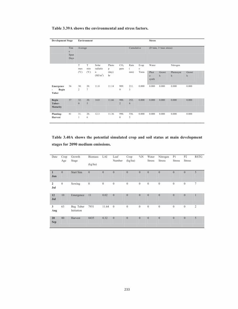
233
Table 3.39A shows the environmental and stress factors.
Development Stage Environment Stress
Time Span Days
Average Cumulative (0=min, 1=max stress)
T max (oC)
T min (oC)
Solar radiation (MJ/m2)
Photop (day) hr
CO2 ppm
Rain ( mm)
Evapo Trans
Water Nitrogen
Photo synth
Growth
Photosynth
Growth
Emergence- Begin Tuber
36 30.2
20.7
11.0 11.14 989.9
211.3
0.000 0.000 0.000 0.000 0.000
Begin Tuber-Maturity
37 32.0
20.5
14.0 11.66 990.2
252.8
0.000 0.000 0.000 0.000 0.000
Planting-Harvest
81 31.1
20.6
12.3 11.36 990.0
556.5
0.000 0.000 0.000 0.000 0.000
Table 3.40A shows the potential simulated crop and soil status at main development
stages for 2090 medium emissions.
Date Crop
Age Growth Stage
Biomass
(kg\ha)
LAI Leaf Number
Crop (kg\ha)
%N Water Stress
Nitrogen Stress
P1 Stress
P2 Stress
RSTG
1 Jun
0 Start Sim 0 0 0 0 0 0 0 0 0 5
2 Jul
0 Sowing 0 0 0 0 0 0 0 0 0 7
12 Jul
10 Emergence 11 0.02 0 0 0 0 0 0 0 1
3 Aug
63 Beg Tuber Initiation
7931 11.64 0 0 0 0 0 0 0 2
20 Sep
80 Harvest 8435 8.32 0 0 0 0 0 0 0 5

234
Table 3.41A shows the environmental and stress factors.
Development Stage Environment Stress
Time Span Days
Average Cumulative (0=min, 1=max stress)
T max (oC)
T min (oC)
Solar radiation (MJ/m2)
Photop (day) hr
CO2 ppm
Rain ( mm)
Evapo Trans
Water Nitrogen
Photo synth
Growth
Photosynth
Growth
Emergence- Begin Tuber
53 32.0
21.6
13.2 11.28 700.0
352.1
0.000 0.000 0.000 0.000 0.000
Begin Tuber-Maturity
18 33.5
22.1
11.2 11.82 700.0
106.0
0.000 0.000 0.000 0.000 0.000
Planting-Harvest
81 32.3
21.8
12.3 11.36 700.0
561.2
0.000 0.000 0.000 0.000 0.000
Table 3.42A shows the potential simulated crop and soil status at main development
stages for 2090 high emissions.
Date Crop
Age Growth Stage
Biomass
(kg\ha)
LAI Leaf Number
Crop (kg\ha)
%N Water Stress
Nitrogen Stress
P1 Stress
P2 Stress
RSTG
1 Jun
0 Start Sim 0 0 0 0 0 0 0 0 0 5
2 Jul
0 Sowing 0 0 0 0 0 0 0 0 0 7
13 Jul
11 Emergence 11 0.02 0 0 0 0 0 0 0 1
9 Sep
69 Beg Tuber Initiation
10035 14.46 0 0 0 0 0 0 0 2
20 Sep
80 Harvest 8810 9.23 0 0 0 0 0 0 0 5

235
Table 3.43A shows the environmental and stress factors.
Development Stage Environment Stress
Time Span Days
Average Cumulative (0=min, 1=max stress)
T max (oC)
T min (oC)
Solar radiation (MJ/m2)
Photop (day) hr
CO2 ppm
Rain ( mm)
Evapo Trans
Water Nitrogen
Photo synth
Growth
Photosynth
Growth
Emergence- Begin Tuber
58 32.1
21.9
13.1 11.33 950.0
408.8
0.000 0.000 0.000 0.000 0.000
Begin Tuber-Maturity
12 35.0
23.0
11.0 11.87 950.0
64.1 0.000 0.000 0.000 0.000 0.000
Planting-Harvest
81 32.6
22.1
12.3 11.36 950.0
580.2
0.000 0.000 0.000 0.000 0.000
3.1.6A Nacocolevu non-potential yield
Table 3.44A shows the potential simulated crop and soil status at main development
stages for 2030 medium emissions.
Date Crop
Age Growth Stage
Biomass
(kg\ha)
LAI Leaf Number
Crop (kg\ha)
%N Water Stress
Nitrogen Stress
P1 Stress
P2 Stress
RSTG
1 Jun
0 Start Sim 0 0 0 0 0 0 0 0 0 5
2 Jul
0 Sowing 0 0 0 0 0 0 0 0 0 7
10 Jul
8 Emergence 11 0.01 0 5 42.8 0 0 0 0 1
11 Aug
40 Beg Tuber Initiation
1164 1.76 0 551 47.4 0 0.07 0 0 2
20 Sep
80 Harvest 7115 2.85 0 1330 18.7 0 0.18 0 0 5

236
Table 3.45A shows the environmental and stress factors.
Development Stage Environment Stress
Time Span Days
Average Cumulative (0=min, 1=max stress)
T max (oC)
T min (oC)
Solar radiation (MJ/m2)
Photop (day) hr
CO2 ppm
Rain ( mm)
Evapo Trans
Water Nitrogen
Photo synth
Growth
Photosynth
Growth
Emergence- Begin Tuber
32 29.7
20.5
10.3 11.11 490.0
184.5
90.2 0.000 0.000 0.047 0.071
Begin Tuber-Maturity
41 31.4
19.7
14.2 11.63 490.0
263.7
138.6 0.000 0.000 0.141 0.177
Planting-Harvest
81 30.6
20.1
12.3 11.36 490.0
537.4
249.0 0.000 0.000 0.090 0.118
Table 3.46A shows the potential simulated crop and soil status at main development
stages for 2030 high emissions.
Date Crop
Age Growth Stage
Biomass
(kg\ha)
LAI Leaf Number
Crop (kg\ha)
%N Water Stress
Nitrogen Stress
P1 Stress
P2 Stress
RSTG
1 Jun
0 Start Sim 0 0 0 0 0 0 0 0 0 5
2 Jul
0 Sowing 0 0 0 0 0 0 0 0 0 7
10 Jul
8 Emergence 11 0.01 0 5 42.8 0 0 0 0 1
10 Aug
39 Beg Tuber Initiation
1073 1.64 0 500 46.6 0 0.07 0 0 2
20 Sep
80 Harvest 7501 2.50 0 1298 17.3 0 0.21 0 0 5

237
Table 3.47A shows the environmental and stress factors.
Development Stage Environment Stress
Time Span Days
Average Cumulative (0=min, 1=max stress)
T max (oC)
T min (oC)
Solar radiation (MJ/m2)
Photop (day) hr
CO2 ppm
Rain ( mm)
Evapo Trans
Water Nitrogen
Photo synth
Growth
Photosynth
Growth
Emergence- Begin Tuber
31 29.4
20.4
10.1 11.11 520.0
184.0
85.6 0.000 0.000 0.047 0.072
Begin Tuber-Maturity
42 31.2
19.4
14.3 11.62 520.0
272.2
142.4 0.000 0.000 0.171 0.204
Planting-Harvest
81 30.4
19.9
12.3 11.36 520.0
546.9
248.1 0.000 0.000 0.107 0.133
Table 3.48A shows the potential simulated crop and soil status at main development
stages for 2055 medium emissions.
Date Crop
Age Growth Stage
Biomass
(kg\ha)
LAI Leaf Number
Crop (kg\ha)
%N Water Stress
Nitrogen Stress
P1 Stress
P2 Stress
RSTG
1 Jun
0 Start Sim 0 0 0 0 0 0 0 0 0 5
2 Jul
0 Sowing 0 0 0 0 0 0 0 0 0 7
11 Jul
9 Emergence 11 0.01 0 5 42.9 0 0 0 0 1
16 Aug
45 Beg Tuber Initiation
1933 2.95 0 819 42.4 0 0.07 0 0 2
20 Sep
80 Harvest 5703 4.88 0 1302 22.8 0 0.33 0 0 5

238
Table 3.49A shows the environmental and stress factors.
Development Stage Environment Stress
Time Span Days
Average Cumulative (0=min, 1=max stress)
T max (oC)
T min (oC)
Solar radiation (MJ/m2)
Photop (day) hr
CO2 ppm
Rain ( mm)
Evapo Trans
Water Nitrogen
Photo synth
Growth
Photosynth
Growth
Emergence- Begin Tuber
36 30.5
20.7
11.3 11.15 550.0
215.2
110.2 0.000 0.000 0.044 0.064
Begin Tuber-Maturity
36 32.2
20.8
13.9 11.67 550.0
240.9
118.7 0.000 0.000 0.285 0.321
Planting-Harvest
81 31.3
20.8
12.3 11.36 550.0
556.5
251.2 0.000 0.000 0.146 0.171
Table 3.50A shows the potential simulated crop and soil status at main development
stages for 2055 high emissions.
Date Crop
Age Growth Stage
Biomass
(kg\ha)
LAI Leaf Number
Crop (kg\ha)
%N Water Stress
Nitrogen Stress
P1 Stress
P2 Stress
RSTG
1 Jun
0 Start Sim 0 0 0 0 0 0 0 0 0 5
2 Jul
0 Sowing 0 0 0 0 0 0 0 0 0 7
11 Jul
9 Emergence 11 0.01 0 5 42.9 0 0 0 0 1
15 Aug
44 Beg Tuber Initiation
2257 3.44 0 869 38.5 0 0.08 0 0 2
20 Sep
80 Harvest 6099 4.01 0 1273 20.9 0 0.37 0 0 5
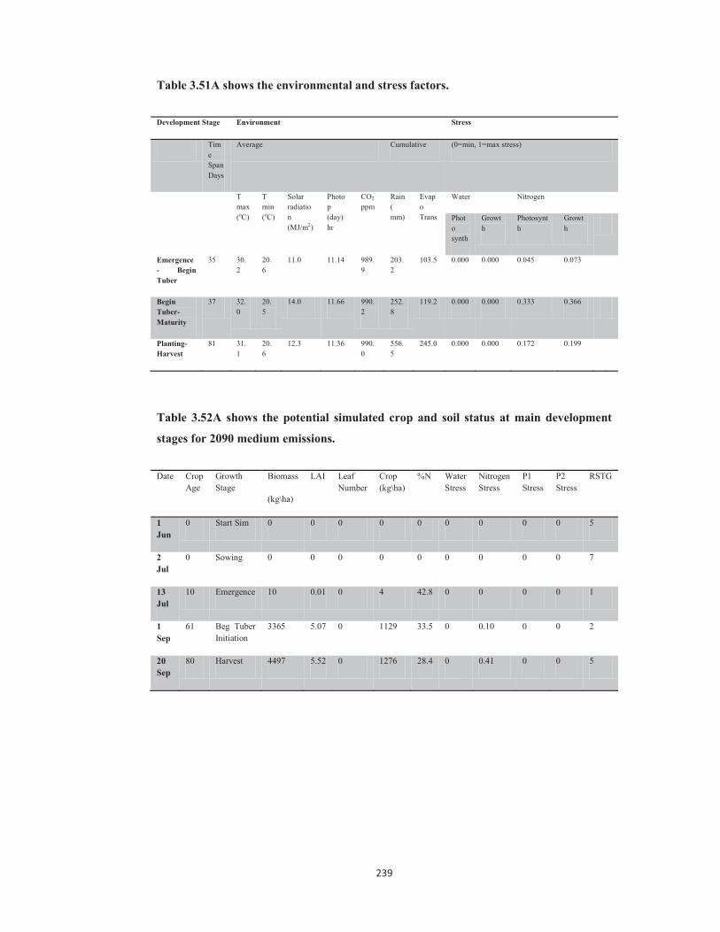
239
Table 3.51A shows the environmental and stress factors.
Development Stage Environment Stress
Time Span Days
Average Cumulative (0=min, 1=max stress)
T max (oC)
T min (oC)
Solar radiation (MJ/m2)
Photop (day) hr
CO2 ppm
Rain ( mm)
Evapo Trans
Water Nitrogen
Photo synth
Growth
Photosynth
Growth
Emergence- Begin Tuber
35 30.2
20.6
11.0 11.14 989.9
203.2
103.5 0.000 0.000 0.045 0.073
Begin Tuber-Maturity
37 32.0
20.5
14.0 11.66 990.2
252.8
119.2 0.000 0.000 0.333 0.366
Planting-Harvest
81 31.1
20.6
12.3 11.36 990.0
556.5
245.0 0.000 0.000 0.172 0.199
Table 3.52A shows the potential simulated crop and soil status at main development
stages for 2090 medium emissions.
Date Crop
Age Growth Stage
Biomass
(kg\ha)
LAI Leaf Number
Crop (kg\ha)
%N Water Stress
Nitrogen Stress
P1 Stress
P2 Stress
RSTG
1 Jun
0 Start Sim 0 0 0 0 0 0 0 0 0 5
2 Jul
0 Sowing 0 0 0 0 0 0 0 0 0 7
13 Jul
10 Emergence 10 0.01 0 4 42.8 0 0 0 0 1
1 Sep
61 Beg Tuber Initiation
3365 5.07 0 1129 33.5 0 0.10 0 0 2
20 Sep
80 Harvest 4497 5.52 0 1276 28.4 0 0.41 0 0 5

240
Table 3.53A shows the environmental and stress factors.
Development Stage Environment Stress
Time Span Days
Average Cumulative (0=min, 1=max stress)
T max (oC)
T min (oC)
Solar radiation (MJ/m2)
Photop (day) hr
CO2 ppm
Rain ( mm)
Evapo Trans
Water Nitrogen
Photo synth
Growth
Photosynth
Growth
Emergence- Begin Tuber
50 32.0
21.7
13.3 11.27 700.0
345.3
174.4 0.000 0.000 0.068 0.094
Begin Tuber-Maturity
20 33.1
22.1
11.4 11.80 700.0
112.1
54.0 0.000 0.000 0.372 0.403
Planting-Harvest
81 32.3
21.8
12.3 11.36 700.0
561.2
255.5 0.000 0.000 0.134 0.158
Table 3.54A shows the potential simulated crop and soil status at main development
stages for 2090 high emissions.
Date Crop
Age Growth Stage
Biomass
(kg\ha)
LAI Leaf Number
Crop (kg\ha)
%N Water Stress
Nitrogen Stress
P1 Stress
P2 Stress
RSTG
1 Jun
0 Start Sim 0 0 0 0 0 0 0 0 0 5
2 Jul
0 Sowing 0 0 0 0 0 0 0 0 0 7
13 Jul
11 Emergence 10 0.01 0 4 42.8 0 0 0 0 1
3 Sep
63 Beg Tuber Initiation
3469 5.22 0 1123 32.4 0 0.13 0 0 2
20 Sep
80 Harvest 4337 5.58 0 1239 28.6 0 0.48 0 0 5

241
Table 3.55A shows the environmental and stress factors.
Development Stage Environment Stress
Time Span Days
Average Cumulative (0=min, 1=max stress)
T max (oC)
T min (oC)
Solar radiation (MJ/m2)
Photop (day) hr
CO2 ppm
Rain ( mm)
Evapo Trans
Water Nitrogen
Photo synth
Growth
Photosynth
Growth
Emergence- Begin Tuber
52 32.2
20.0
13.3 11.28 950.0
363.3
177.8 0.000 0.000 0.095 0.123
Begin Tuber-Maturity
18 33.8
22.4
11.2 11.82 950.0
109.6
49.7 0.000 0.000 0.443 0.470
Planting-Harvest
81 32.6
22.1
12.3 11.36 950.0
580.2
254.7 0.000 0.000 0.160 0.184
3.2A Optimisation treatments
3.2.1A Banisogosogo optimisation
Table 3.56A shows the yield at different planting time for Banisogosogo under A1B and
A2 under non-potential simulations.
Yield (kg/ha)
Planting Time 2030 A1B Emission
2030 A2 Emission
2055 A1B Emission
2055 A2 Emission
January 2 0 0 0 0
February 1 0 0 0 0
March 1 0 0 0 0
April 1 1 0 0 0
May 1 1020 1688 0 245
June 1 1931 2571 271 855
July 2 (default run)
2116 2469 757 1423
August 1 1249 1812 168 606
September 1 501 574 234 398

242
October 1 1511 1763 361 836
November 1 0 0 0 0
December 1 103 0 0 0
Table 3.57A shows the yield at different row spacing for Banisogosogo under A1B and
A2 under non-potential simulations.
Yield (kg/ha)
Row Spacing ( cm)
Plant Population (m2)
2030 A1B Emission
2030 A2 Emission
2055 A1B Emission
2055 A2 Emission
75(default run) 5 1261 2713 148 300
30 11 1229 2768 188 302
40 8 1246 2803 148 301
50 6 1256 2713 148 300
80 4 1171 2713 148 300
100 3 1174 2712 147 299
Table 3.58A shows the yield under different irrigation amount for Banisogosogo under
A1B and A2 non-potential simulations.
Yield (kg/ha)
Irrigation ( mm)
2030 A1B Emission 2030 A2 Emission 2055 A1B Emission 2055 A2 Emission
Default run (1.6 mm and 4.0 mm)
1261 2713 148 300
1.6 1194 1822 82 301
4.0 1209 1867 54 241
6.4 1138 1869 38 187
8.0 1135 1722 23 182
9.6 1124 1579 23 184
12.0 1063 1576 23 186
14.4 1127 1585 24 184
16.0 1129 1580 24 184

243
Table 3.59A shows the planting depth with corresponding yield for Banisogosogo under
A1B and A2 non-potential simulations.
Yield (kg/ha)
Planting Depth ( cm) 2030 A1B Emission 2030 A2 Emission 2055 A1B Emission 2055 A2 Emission
1.5 1261 1166 1166 300
2 977 1135 1135 140
4 235 1196 1196 0
6 6 1166 720 0
8 0 32 32 0
10 0 0 0 0
Table 3.60A shows the application of fertiliser (banded beneath surface at different
depth) and corresponding yield for Banisogosogo 2030 A1B emission.
Yield (kg/ha) at depth
Default run (80 N kg/ha in 2 splits at 5 cm)
1261
Fertiliser (kg/ha) 0 cm 2 cm 4 cm 6 cm 8 cm 10 cm
60 1260 1260 1260 1251 1240 1233
120 1223 1223 1223 1212 1198 1192
180 1234 1234 1234 1233 1224 1217
240 1212 1212 1212 1209 1138 1139
300 1410 1410 1410 1395 1175 1123
.

244
Table 3.61A shows the optimum fertiliser and irrigation management for Banisogosogo
2030 A1B emission.
Optimum Fertiliser and Irrigation Management
Fertiliser Application (kg/ha at x cm) Irrigation Application ( mm) Yield (kg/ha)
300 at 0 cm Default value 1475
300at 2 cm Default value 1475
300 at 4 cm Default value 1475
Table 3.62A shows the application of fertiliser (banded beneath surface) and
corresponding yield for Banisogosogo 2030 A2 emission.
Yield (kg/ha) at depth
Default run (80 N kg/ha in 2 splits at 5 cm)
1166
Fertiliser (kg/ha) 0 cm 2 cm 4 cm 6 cm 8 cm 10 cm
60 1759 1759 1759 1742 1726 1720
120 1867 1867 1867 1843 1821 1812
180 1930 1930 1930 1906 1877 1731
240 1937 1937 1937 2021 1768 1763
300 2265 2265 2265 2092 1867 1792
Table 3.63A shows the optimum fertiliser and irrigation management for Banisogosogo
2030 A2 Emission.
Optimum Fertiliser and Irrigation Management
Fertiliser Application (kg/ha at x cm) Irrigation Application ( mm) Yield (kg/ha)
300 at 0 cm Default value 2221
300at 2 cm Default value 2221
300 at 4 cm Default value 2221

245
Table 3.64A shows the application of fertiliser (banded beneath surface at different
depth) and corresponding yield for Banisogosogo 2055 A1B Emission.
Yield (kg/ha) at depth
Default run (80 N kg/ha in 2 splits at 5 cm)
1166
Fertiliser (kg/ha) 0 cm 2 cm 4 cm 6 cm 8 cm 10 cm
60 119 119 119 119 119 119
120 96 96 96 96 97 97
180 78 78 78 80 80 80
240 62 62 62 65 37 36
300 33 33 33 21 12 12
Table 3.65A shows the optimum fertiliser and irrigation management for Banisogosogo
2055 A1B emission.
Optimum Fertiliser and Irrigation Management
Fertiliser Application Irrigation Application ( mm) Yield (kg/ha)
Default value Default value 82
Table 3.66A shows the application of fertiliser (banded beneath surface at different
depth) and corresponding yield for Banisogosogo 2055 A2 emission.
Yield (kg/ha) at depth
Default run (80 N kg/ha in 2 splits at 5 cm)
300
Fertiliser (kg/ha) 0 cm 2 cm 4 cm 6 cm 8 cm 10 cm
60 304 304 304 303 303 303
120 300 300 300 300 301 301
180 294 294 294 296 238 237
240 224 224 224 229 226 178
300 197 197 197 167 165 133

246
Table 3.67A shows the optimum fertiliser and irrigation management for Banisogosogo
2055 A2 emission.
Optimum Fertiliser and Irrigation Management
Fertiliser Application (kg/ha at x cm) Irrigation Application ( mm) Yield (kg/ha)
60 kg/ha at 0 cm 1.6 292
60 kg/ha at 2 cm 1.6 292
60 kg/ha at 4 cm 1.6 292
3.2.2A Koronivia Optimisation Treatments
Table 3.68A shows the yield at different planting time for Koronivia for 2030-2090
under A1B and A2 emission scenario.
Yield (kg/ha)
Planting Time
2030 A1B Emission
2030 A2 Emission
2055 A1B Emission
2055 A2 Emission
2090 A1B Emission
2090 A2 Emission
January 2 0 0 0 0 0 0
February 1 0 0 0 0 0 0
March 1 33 292 0 0 0 0
April 1 1655 2245 864 1524 0 0
May 1 3334 3914 2213 3191 833 583
June 1 3457 4249 2587 3923 1123 897
July 2 (default run)
4268 5368 3205 4799 1911 1570
August 1 6692 7827 3590 5961 1117 745
September 1 3692 4255 2515 3609 1485 1128
October 1 2953 3710 1324 2230 235 32
November 1 334 502 36 193 0 0
December 1 139 196 4 62 0 0
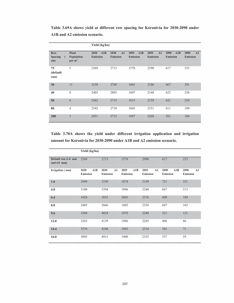
247
Table 3.69A shows yield at different row spacing for Koronivia for 2030-2090 under
A1B and A2 emission scenario.
Yield (kg/ha)
Row Spacing ( cm)
Plant Population per m2
2030 A1B Emission
2030 A2 Emission
2055 A1B Emission
2055 A2 Emission
2090 A1B Emission
2090 A2 Emission
75 (default run)
5 2369 2713 1578 2290 617 233
30 11 2358 2768 1601 2186 667 291
40 8 2403 2803 1607 2148 625 238
50 6 2362 2713 1615 2159 621 234
80 4 2342 2718 1665 2331 611 188
100 3 2451 2712 1687 2268 561 186
Table 3.70A shows the yield under different irrigation application and irrigation
amount for Koronivia for 2030-2090 under A1B and A2 emission scenario.
Yield (kg/ha)
Default run (1.6 mm and 4.0 mm)
2369 2713 1578 2990 617 233
Irrigation ( mm) 2030 A1B Emission
2030 A2 Emission
2055 A1B Emission
2055 A2 Emission
2090 A1B Emission
2090 A2 Emission
1.6 2949 3330 1874 2159 721 251
4.0 3180 3394 1896 2240 687 213
6.4 3428 3855 2005 2376 609 189
8.0 3485 3866 1885 2354 607 165
9.6 3568 4024 1870 2240 521 121
12.0 3263 4139 1886 2245 406 86
14.4 3576 4548 1882 2314 341 71
16.0 3885 4911 1908 2335 337 59

248
Table 3.71A shows the planting depth with corresponding yield for Koronivia for 2030-
2090 under A1B and A2 emission scenario.
Yield (kg/ha)
Planting Depth ( cm)
2030 A1B Emission
2030 A2 Emission
2055 A1B Emission
2055 A2 Emission
2090 A1B Emission
2090 A2 Emission
1.5 (default run)
2369 2713 1578 2290 617 233
2 2255 2581 1503 2052 241 25
4 2067 2415 1077 1503 0 0
6 1804 2183 181 579 0 0
8 122 450 0 0 0 0
10 0 0 0 0 0 0
Table 3.72A shows the application of fertiliser (banded beneath surface at different
depth) and corresponding yield for Koronivia under 2030 A1B emission.
Yield (kg/ha) at depth
Default run (80 N kg/ha in 2 splits at 5 cm)
2369
Fertiliser (kg/ha) 0 cm 2 cm 4 cm 6 cm 8 cm 10 cm
60 2860 2860 2860 2844 2849 2842
120 2881 2881 2881 2867 2855 2852
180 2820 2820 2820 2774 2770 2767
240 2751 2751 2751 2750 2742 2739
300 2914 2914 2914 2878 2876 2890

249
Table 3.73A shows the optimum fertiliser and irrigation management for Koronivia
under 2030 A1B emission.
Optimum Fertiliser and Irrigation Management
Fertiliser Application (kg/ha at x cm) Irrigation Application ( mm) Yield (kg/ha)
300 kg/ha at 0 cm 16.0 3750
300 kg/ha at 2 cm 16.0 3449
300 kg/ha at 4 cm 16.0 2933
Table 3.74A shows the application of fertiliser (banded beneath surface at different
depth) and corresponding yield for Koronivia under 2030 A2 emission.
Yield (kg/ha) at depth
Default run (80 N kg/ha in 2 splits at 5 cm)
2713
Fertiliser (kg/ha) 0 cm 2 cm 4 cm 6 cm 8 cm 10 cm
60 3217 3217 3217 3194 3176 3166
120 3341 3341 3341 3302 3270 3255
180 3249 3249 3249 3227 3202 3224
240 3248 3248 3248 3148 3127 3115
300 3400 3400 3400 3281 3259 3282
Table 3.75A shows the optimum fertiliser and irrigation management for Koronivia
under 2030 A2 emission.
Optimum Fertiliser and Irrigation Management
Fertiliser Application (kg/ha at x cm) Irrigation Application ( mm) Yield (kg/ha)
300 kg/ha at 0 cm 16 4342
300 kg/ha at 2 cm 16 4047
300 kg/ha at 4 cm 16 3245

250
Table 3.76A shows the application of fertiliser (banded beneath surface at different
depth) and corresponding yield for Koronivia under 2055 A1B emission.
Yield (kg/ha) at depth
Default run (80 N kg/ha in 2 splits at 5 cm)
1578
Fertiliser (kg/ha) 0 cm 2 cm 4 cm 6 cm 8 cm 10 cm
60 2014 2014 2014 2010 2003 2001
120 1903 1903 1903 1897 1890 1883
180 1838 1838 1838 1840 1831 1830
240 1816 1816 1816 1813 1849 1848
300 1921 1921 1921 1948 1826 1817
Table 3.77A shows the optimum fertiliser and irrigation management for Koronivia
under 2055 A1B emission.
Optimum Fertiliser and Irrigation Management
Fertiliser Application (kg/ha at x cm) Irrigation Application ( mm) Yield (kg/ha)
60 kg/ha at 0 cm 6.4 1932
60kg/ha at 2 cm 6.4 1927
60kg/ha at 4 cm 6.4 1811

251
Table 3.78A shows the application of fertiliser (banded beneath surface at different
depth) and corresponding yield for Koronivia under 2055 A2 emission.
Yield (kg/ha) at depth
Default run (80 N kg/ha in 2 splits at 5 cm)
2990
Fertiliser (kg/ha) 0 cm 2 cm 4 cm 6 cm 8 cm 10 cm
60 2307 2307 2307 2299 2290 2287
120 2185 2185 2185 2170 2159 2154
180 2122 2122 2122 2118 2113 2111
240 2073 2073 2073 2128 2118 2115
300 2114 2114 2114 2232 2227 2253
Table 3.79A shows the optimum fertiliser and irrigation management for Koronivia
under 2055 A2 emission.
Optimum Fertiliser and Irrigation Management
Fertiliser Application (kg/ha at x cm) Irrigation Application ( mm) Yield (kg/ha)
Default run Default run 2100
Table 3.80A shows the application of fertiliser (banded beneath surface at different
depth) and corresponding yield for Koronivia under 2090 A1B emission.
Yield (kg/ha) at depth
Default run (80 N kg/ha in 2 splits at 5 cm)
617
Fertiliser (kg/ha) 0 cm 2 cm 4 cm 6 cm 8 cm 10 cm
60 772 772 772 772 773 773
120 761 761 761 761 761 760
180 746 746 746 754 750 754
240 705 705 705 756 756 756
300 693 693 693 749 754 755

252
Table 3.81A shows the optimum fertiliser and irrigation management for Koronivia
under 2090 A1B emission.
Optimum Fertiliser and Irrigation Management
Fertiliser Application (kg/ha at x cm) Irrigation Application ( mm) Yield (kg/ha)
60 kg/ha at 8 cm 1.6 779
60 kg/ha at 10 cm 1.6 779
Table 3.82A shows the application of fertiliser (banded beneath surface at different
depth) and corresponding yield for Koronivia under 2090 A2 emission.
Yield (kg/ha) at depth
Default run (80 N kg/ha in 2 splits at 5 cm)
233
Fertiliser (kg/ha) 0 cm 2 cm 4 cm 6 cm 8 cm 10 cm
60 351 351 351 351 350 351
120 245 245 245 245 295 295
180 296 296 296 296 296 296
240 243 243 243 244 244 244
300 240 240 240 241 242 242
Table 3.83A shows the optimum fertiliser and irrigation management for Koronivia
under 2090 A2 emission.
Optimum Fertiliser and Irrigation Management
Fertiliser Application (kg/ha at x cm) Irrigation Application ( mm) Yield (kg/ha)
60 kg/ha at 0 cm 1.6 401
60 kg/ha at 2 cm 1.6 401
60 kg/ha at 4 cm 1.6 401
60 kg/ha at 6 cm 1.6 357
60 kg/ha at 8 cm 1.6 357

253
3.2.3A Nacocolevu Optimisation Treatments
Table 3.84A shows the yield at different planting time for Nacocolevu for 2030-2090
A1B and A2 emission scenario.
Yield (kg/ha)
Planting Time
2030 A1B Emission
2030 A2 Emission
2055 A1B Emission
2055 A2 Emission
2090 A1B Emission
2090 A2 Emission
January 2 0 0 0 0 0 0
February 1 0 0 0 0 0 0
March 1 52 179 0 0 0 0
April 1 3635 4369 1094 1826 2 0
May 1 5670 5876 4887 5593 1416 971
June 1 7066 6900 8141 9385 4729 3421
July 2 (default run)
7476 7523 6222 7580 3792 3634
August 1 8178 8522 6090 7547 3399 3205
September 1 5081 5674 3385 4547 1573 1072
October 1 2207 2796 1199 2006 432 288
November 1 1081 1448 158 595 0 0
December 1 0 0 0 0 0 0
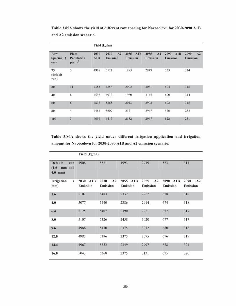
254
Table 3.85A shows the yield at different row spacing for Nacocolevu for 2030-2090 A1B
and A2 emission scenario.
Yield (kg/ha)
Row Spacing ( cm)
Plant Population per m2
2030 A1B
2030 A2 Emission
2055 A1B Emission
2055 A2 Emission
2090 A1B Emission
2090 A2 Emission
75 (default run)
5 4908 5521 1993 2949 523 314
30 11 4385 4856 2002 3031 604 315
40 8 4598 4932 1960 3145 600 314
50 6 4833 5365 2013 2902 602 315
80 4 4484 5609 2121 2947 526 252
100 3 4694 6417 2182 2947 522 251
Table 3.86A shows the yield under different irrigation application and irrigation
amount for Nacocolevu for 2030-2090 A1B and A2 emission scenario.
Yield (kg/ha)
Default run (1.6 mm and 4.0 mm)
4908 5521 1993 2949 523 314
Irrigation ( mm)
2030 A1B Emission
2030 A2 Emission
2055 A1B Emission
2055 A2 Emission
2090 A1B Emission
2090 A2 Emission
1.6 5102 5483 2332 2957 678 318
4.0 5077 5440 2386 2914 674 318
6.4 5125 5407 2390 2951 672 317
8.0 5107 5326 2458 3020 677 317
9.6 4988 5430 2375 3012 680 318
12.0 4985 5396 2375 3075 676 319
14.4 4967 5352 2349 2997 678 321
16.0 5043 5368 2375 3131 675 320

255
Table 3.87A shows the planting depth with corresponding yield for Nacocolevu for
2030-2090 A1B and A2 emission scenario.
Yield (kg/ha)
Planting Depth ( cm)
2030 A1B Emission
2030 A2 Emission
2055 A1B Emission
2055 A2 Emission
2090 A1B Emission
2090 A2 Emission
1.5 (default run)
4908 5521 1993 2949 523 314
2 3525 4793 1768 2394 341 157
4 1996 2284 929 1431 3 0
6 1255 1570 363 777 0 0
8 449 883 0 12 0 0
Table 3.88A shows the application of fertiliser (banded beneath surface at different
depth) and corresponding yield for Nacocolevu under 2030 A1B emission scenario.
Yield (kg/ha) at depth
Default run (80 N kg/ha in 2 splits at 5 cm)
4908
Fertiliser (kg/ha) 0 cm 2 cm 4 cm 6 cm 8 cm 10 cm
60 3030 3030 3030 3147 3300 3470
120 4598 4598 4598 4793 4836 4838
180 4902 4902 4902 4924 4803 4707
240 4799 4799 4799 4578 4726 4715
300 4690 4690 4690 4867 4997 4984

256
Table 3.89A shows the optimum fertiliser and irrigation management for Nacocolevu
under 2030 A1B emission scenario.
Optimum Fertiliser and Irrigation Management
Fertiliser Application (kg/ha at x cm) Irrigation Application ( mm) Yield (kg/ha)
300 kg/ha at 8 cm 6.4 5818
Table 3.90A shows the application of fertiliser (banded beneath surface at different
depth) and corresponding yield for Nacocolevu under 2030 A2 emission scenario.
Yield (kg/ha) at depth
Default run (80 N kg/ha in 2 splits at 5 cm)
5611
Fertiliser (kg/ha) 0 cm 2 cm 4 cm 6 cm 8 cm 10 cm
60 2966 2966 2966 3103 3255 3364
120 4589 4589 4589 4554 4844 4911
180 5107 5107 5107 5146 5204 5054
240 5138 5138 5138 4943 5189 5259
300 5332 5332 5332 5398 5404 5473
Table 3.91A shows the optimum fertiliser and irrigation management for Nacocolevu
under 2030 A2 emission scenario.
Optimum Fertiliser and Irrigation Management
Fertiliser Application (kg/ha at 10 cm) Irrigation Application ( mm) Yield (kg/ha)
Default run Default run 5549
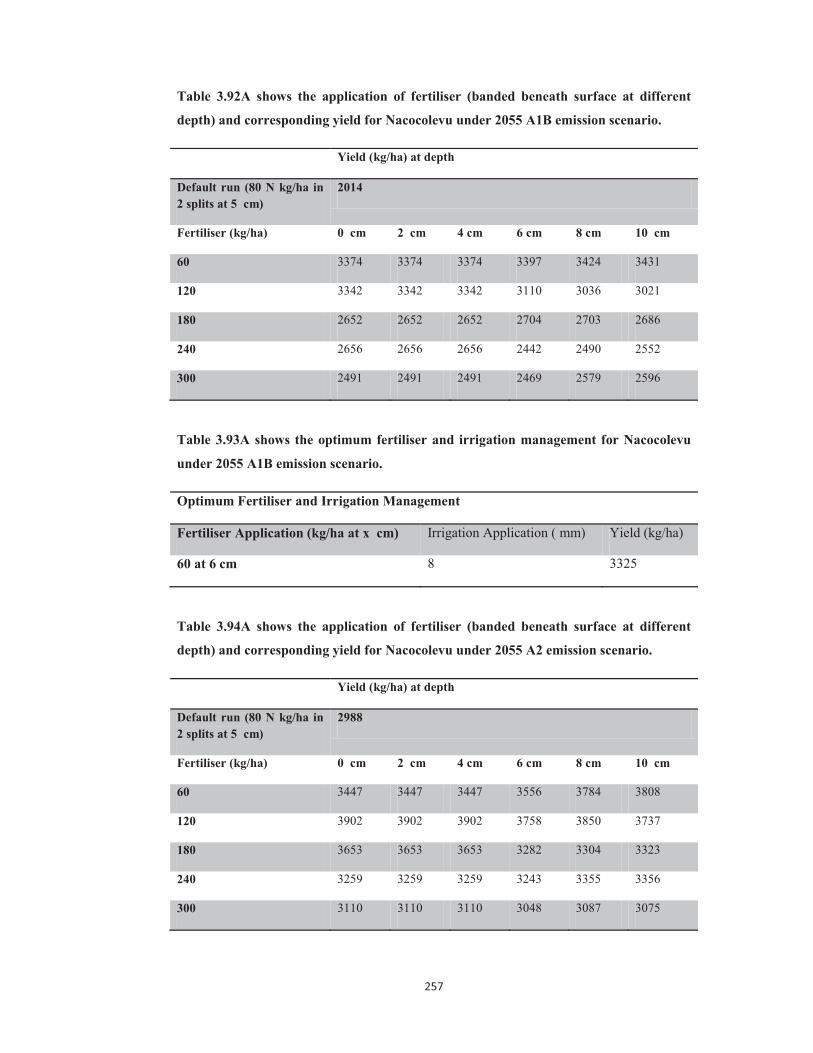
257
Table 3.92A shows the application of fertiliser (banded beneath surface at different
depth) and corresponding yield for Nacocolevu under 2055 A1B emission scenario.
Yield (kg/ha) at depth
Default run (80 N kg/ha in 2 splits at 5 cm)
2014
Fertiliser (kg/ha) 0 cm 2 cm 4 cm 6 cm 8 cm 10 cm
60 3374 3374 3374 3397 3424 3431
120 3342 3342 3342 3110 3036 3021
180 2652 2652 2652 2704 2703 2686
240 2656 2656 2656 2442 2490 2552
300 2491 2491 2491 2469 2579 2596
Table 3.93A shows the optimum fertiliser and irrigation management for Nacocolevu
under 2055 A1B emission scenario.
Optimum Fertiliser and Irrigation Management
Fertiliser Application (kg/ha at x cm) Irrigation Application ( mm) Yield (kg/ha)
60 at 6 cm 8 3325
Table 3.94A shows the application of fertiliser (banded beneath surface at different
depth) and corresponding yield for Nacocolevu under 2055 A2 emission scenario.
Yield (kg/ha) at depth
Default run (80 N kg/ha in 2 splits at 5 cm)
2988
Fertiliser (kg/ha) 0 cm 2 cm 4 cm 6 cm 8 cm 10 cm
60 3447 3447 3447 3556 3784 3808
120 3902 3902 3902 3758 3850 3737
180 3653 3653 3653 3282 3304 3323
240 3259 3259 3259 3243 3355 3356
300 3110 3110 3110 3048 3087 3075

258
Table 3.95A shows the optimum fertiliser and irrigation management for Nacocolevu
under 2055 A2 emission scenario.
Optimum Fertiliser and Irrigation Management
Fertiliser Application (kg/ha at x cm) Irrigation Application ( mm) Yield (kg/ha)
60 kg/ha at 10 cm 16 mm 3751
Table 3.96A shows the application of fertiliser (banded beneath surface at different
depth) and corresponding yield for Nacocolevu under 2090 A1B emission scenario.
Yield (kg/ha) at depth
Default run (80 N kg/ha in 2 splits at 5 cm)
519
Fertiliser (kg/ha) 0 cm 2 cm 4 cm 6 cm 8 cm 10 cm
60 1144 1144 1144 1118 1117 1107
120 1086 1086 1086 1083 1078 1074
180 962 962 962 966 965 867
240 851 851 851 850 830 831
300 846 846 846 827 734 683
Table 3.97A shows the optimum fertiliser and irrigation management for Nacocolevu
under 2090 A1B emission scenario.
Optimum Fertiliser and Irrigation Management
Fertiliser Application (kg/ha at x cm) Irrigation Application ( mm) Yield (kg/ha)
60 kg/ha at 0 cm 9.6 974
60 kg/ha at 2 cm 9.6 974
60 kg/ha at 4 cm 9.6 974

259
Table 3.98A shows the application of fertiliser (banded beneath surface at different
depth) and corresponding yield for Nacocolevu under 2090 A2 emission scenario.
Yield (kg/ha) at depth
Default run (80 N kg/ha in 2 splits at 5 cm)
315
Fertiliser (kg/ha) 0 cm 2 cm 4 cm 6 cm 8 cm 10 cm
60 749 749 749 741 631 629
120 728 728 728 729 726 640
180 539 539 539 450 461 461
240 454 454 454 453 452 432
300 448 448 448 373 355 333
Table 3.99A shows the optimum fertiliser and irrigation management.
Optimum Fertiliser and Irrigation Management
Fertiliser Application (kg/ha at x cm) Irrigation Application ( mm) Yield (kg/ha)
60 kg/ha at 0 cm 16 612
60 kg/ha at 2 cm 16 612
60 kg/ha at 4 cm 16 612

260
Appendix 4: Simulation of other potato varieties
Appendix 4 provides the model output for potential and non-potential for current and
future climate simulations using Sebago and Russet Burbank varieties. The model
simulation was conducted only for Banisogosogo using PCCSP A1B and A2
emission scenarios were used. Likewise, it also shows the optimisation results for
planting date, row spacing, fertiliser application, irrigation application and planting
depth.
4A Cultivar selection
4.1A Sebago current climate simulations
4.1.1 A Banisogosogo potential simulation
Table 4.0A shows the potential simulated crop and soil status at main development
stages for Banisogosogo.
Date Crop
Age Growth Stage
Biomass (kg\ha)
LAI Leaf Number
Crop (kg\ha)
%N Water Stress
Nitrogen Stress
P1 Stress
P2 Stress
RSTG
1 Jun
0 Start Sim 0 0 0 0 0 0 0 0 0 5
2 Jul
0 Sowing 0 0 0 0 0 0 0 0 0 7
9 Jul
7 Emergence 12 0.02 0 0 0 0 0 0 0 1
4 Aug
33 Beg Tuber Initiation
1601 2.43 0 0 0 0 0 0 0 2
20 Sep
80 Harvest 12433 6.14 0 0 0 0 0 0 0 2
Table 4.1A shows the environmental and stress factors.
Development Stage Environment Stress Time
Span Days
Average Cumulative (0=min, 1=max stress)
T max (oC)
T min (oC)
Solar radiation (MJ/m2)
Photop (day) hr
CO2 ppm
Rain ( mm)
Evapo Trans
Water Nitrogen
Photo synth
Growth Photosynth Growth
Emergence- Begin Tuber
26 27.6 20.5 13.9 11.12 392.0 18.2 0.000 0.000 0.000 0.000 0.000
Begin Tuber-Maturity
48 28.9 21.8 17.4 11.61 392.1 64.5 0.000 0.000 0.000 0.000 0.000
Planting-Harvest
81 28.4 21.3 16.2 11.4 392.1 134.3 0.000 0.000 0.000 0.000 0.000

261
4.1.2 A Banisogosogo non-potential simulation
Table 4.2A shows the non-potential simulated crop and soil status at main development
stages for Banisogosogo.
Date Crop
Age Growth Stage
Biomass (kg\ha)
LAI Leaf Number
Crop (kg\ha)
%N Water Stress
Nitrogen Stress
P1 Stress
P2 Stress
RSTG
1 Jun
0 Start Sim 0 0 0 0 0 0 0 0 0 5
2 Jul
0 Sowing 0 0 0 0 0 0 0 0 0 7
9 Jul
7 Emergence 11 0.01 0 5 42.8 0 0 0 0 1
2 Aug
31 Beg Tuber Initiation
251 0.37 0 89 35.5 0 0.16 0 0 2
20 Sep
80 Harvest 2898 0.22 0 520 17.9 0.21 0.03 0 0 2
Table 4.3A shows the environmental and stress factors.
Development Stage Environment Stress Tim
e Span Days
Average Cumulative (0=min, 1=max stress)
T max (oC)
T min (oC)
Solar radiation (MJ/m2)
Photop (day) hr
CO2 ppm
Rain ( mm)
Evapo Trans
Water Nitrogen
Photo synth
Growth
Photosynth
Growth
Emergence- Begin Tuber
24 27.6
20.4
13.6 11.11 392.0
18.2 37.7 0.000 0.000 0.117 0.155
Begin Tuber-Maturity
50 28.8
21.7
17.4 11.59 392.1
115.7
138.7 0.132 0.202 0.009 0.032
Planting-Harvest
80 28.4
21.3
16.2 11.4 392.1
134.3
184.5 0.082 0.125 0.040 0.066
4.2A Russet Burbank current climate simulation
4.2.1 A Banisogosogo potential simulation
Table 4.4A shows the potential simulated crop and soil status at main development
stages for Banisogosogo.
Date Crop
Age Growth Stage
Biomass (kg\ha)
LAI Leaf Number
Crop (kg\ha)
%N Water Stress
Nitrogen Stress
P1 Stress
P2 Stress
RSTG
1 Jun
0 Start Sim 0 0 0 0 0 0 0 0 0 5
2 Jul
0 Sowing 0 0 0 0 0 0 0 0 0 7
9 Jul
7 Emergence 12 0.02 0 0 0 0 0 0 0 1
24 Aug
53 Beg Tuber Initiation
5589 8.33 0 0 0 0 0 0 0 2

262
20 Sep
80 Harvest 9316 7.10 0 0 0 0 0 0 0 2
Table 4.5A shows the environmental and stress factors.
Development Stage Environment Stress Time
Span Days
Average Cumulative (0=min, 1=max stress)
T max (oC)
T min (oC)
Solar radiation (MJ/m2)
Photop (day) hr
CO2 ppm
Rain ( mm)
Evapo Trans
Water Nitrogen Photo synth
Growth Photosynth Growth
Emergence- Begin Tuber
46 28.2 21.0 14.7 11.24 392.0 84.3 0.000 0.000 0.000 0.000 0.000
Begin Tuber-Maturity
48 28.8 21.8 18.6 11.76 392.0 49.6 0.000 0.000 0.000 0.000 0.000
Planting-Harvest
81 28.4 21.3 16.2 11.4 392.1 134..3 0.000 0.000 0.000 0.000 0.000
4.2.2 A Banisogosogo non-potential simulation
Table 4.6A shows non potential simulated crop and soil status at main development
stages for Banisogosogo.
Date Crop
Age Growth Stage
Biomass (kg\ha)
LAI Leaf Number
Crop (kg\ha)
%N Water Stress
Nitrogen Stress
P1 Stress
P2 Stress
RSTG
1 Jun
0 Start Sim 0 0 0 0 0 0 0 0 0 5
2 Jul
0 Sowing 0 0 0 0 0 0 0 0 0 7
9 Jul
7 Emergence 11 0.01 0 5 42.8 0 0 0 0 1
21 Aug
50 Beg Tuber Initiation
2559 3.89 0 1130 44.2 0 0.10 0 0 2
20 Sep
80 Harvest 6239 5.55 0 1878 30.1 0.19 0.07 0 0 2
Table 4.7A shows the environmental and stress factors.
Development Stage Environment Stress Tim
e Span Days
Average Cumulative (0=min, 1=max stress)
T max (oC)
T min (oC)
Solar radiation (MJ/m2)
Photop (day) hr
CO2 ppm
Rain ( mm)
Evapo Trans
Water Nitrogen
Photo synth
Growth
Photosynth
Growth
Emergence- Begin Tuber
43 28.2
21.0
14.6 11.22 392.0
84.1 109.2 0.000 0.000 0.079 0.104
Begin Tuber-Maturity
31 28.7
21.7
18.4 11.74 392.0
49.8 123.6 0.083 0.183 0.021 0.065
Planting-Harvest
80 28.4
21.4
16.2 11.4 392.1
134.3
241.0 0.032 0.070 0.050 0.080

263
4.3A Future climate Sebago simulations
4.3.1A Banisogosogo potential 2030 medium emission scenario
Table 4.8A shows the potential simulated crop and soil status at main development
stages.
Date Crop
Age Growth Stage
Biomass (kg\ha)
LAI Leaf Number
Crop (kg\ha)
%N Water Stress
Nitrogen Stress
P1 Stress
P2 Stress
RSTG
1 Jun
0 Start Sim 0 0 0 0 0 0 0 0 0 5
2 Jul
0 Sowing 0 0 0 0 0 0 0 0 0 7
10 Jul
8 Emergence 12 0.02 0 0 0 0 0 0 0 1
12 Aug
41 Beg Tuber Initiation
2957 4.51 0 0 0 0 0 0 0 2
20 Sep
80 Harvest 9613 6.04 0 0 0 0 0 0 0 2
Table 4.9A shows the environmental and stress factors.
Development Stage Environment Stress Tim
e Span Days
Average Cumulative (0=min, 1=max stress)
T max (oC)
T min (oC)
Solar radiation (MJ/m2)
Photop (day) hr
CO2 ppm
Rain ( mm)
Evapo Trans
Water Nitrogen
Photo synth
Growth
Photosynth
Growth
Emergence- Begin Tuber
33 29.1
21.8
13.9 11.17 490.0
84.8 0.0 0.000 0.000 0.000 0.000
Begin Tuber-Maturity
40 30.1
23.1
18.2 11.67 490.0
65.0 0.0 0.000 0.000 0.000 0.000
Planting-Harvest
81 29.6
22.5
16.2 11.40 490.0
151.8
0.0 0.000 0.000 0.000 0.000
4.3.2 A Banisogosogo potential 2030 high emission scenario
Table 4.10A shows the potential simulated crop and soil status at main development
stages.
Date Crop
Age Growth Stage
Biomass (kg\ha)
LAI Leaf Number
Crop (kg\ha)
%N Water Stress
Nitrogen Stress
P1 Stress
P2 Stress
RSTG
1 Jun
0 Start Sim 0 0 0 0 0 0 0 0 0 5
2 Jul
0 Sowing 0 0 0 0 0 0 0 0 0 7
10 Jul
8 Emergence 12 0.02 0 0 0 0 0 0 0 1
10 Aug
39 Beg Tuber Initiation
2628 4.00 0 0 0 0 0 0 0 2

264
20 Sep
80 Harvest 10236 6.09 0 0 0 0 0 0 0 2
Table 4.11A shows environmental and stress factors.
Development Stage Environment Stress Tim
e Span Days
Average Cumulative (0=min, 1=max stress)
T max (oC)
T min (oC)
Solar radiation (MJ/m2)
Photop (day) hr
CO2 ppm
Rain ( mm)
Evapo Trans
Water Nitrogen
Photo synth
Growth
Photosynth
Growth
Emergence- Begin Tuber
31 28.8
21.7
13.9 11.15 520.0
86.2 0.0 0.000 0.000 0.000 0.000
Begin Tuber-Maturity
42 29.9
22.7
18.0 11.65 520.0
66.1 0.0 0.000 0.000 0.000 0.000
Planting-Harvest
81 29.4
22.3
16.2 11.40 520.0
154.4
0.0 0.000 0.000 0.000 0.000
4.3.3 A Banisogosogo potential 2055 medium emission scenario
Table 4.12A shows the potential simulated crop and soil status at main development
stages.
Date Crop
Age Growth Stage
Biomass (kg\ha)
LAI Leaf Number
Crop (kg\ha)
%N Water Stress
Nitrogen Stress
P1 Stress
P2 Stress
RSTG
1 Jun
0 Start Sim 0 0 0 0 0 0 0 0 0 5
2 Jul
0 Sowing 0 0 0 0 0 0 0 0 0 7
11 Jul
9 Emergence 12 0.02 0 0 0 0 0 0 0 1
24 Aug
53 Beg Tuber Initiation
6068 9.05 0 0 0 0 0 0 0 2
20 Sep
80 Harvest 7949 6.42 0 0 0 0 0 0 0 2
Table 4.13A shows the environmental and stress factors.
Development Stage Environment Stress Tim
e Span Days
Average Cumulative (0=min, 1=max stress)
T max (oC)
T min (oC)
Solar radiation (MJ/m2)
Photop (day) hr
CO2 ppm
Rain ( mm)
Evapo Trans
Water Nitrogen
Photo synth
Growth
Photosynth
Growth
Emergence- Begin Tuber
44 30.2
22.9
14.9 11.25 550.0
97.0 0.0 0.000 0.000 0.000 0.000
Begin Tuber-Maturity
28 30.7
23.7
18.6 11.76 550.0
58.0 0.0 0.000 0.000 0.000 0.000
Planting- 81 30. 23. 16.2 11.40 550. 157. 0.0 0.000 0.000 0.000 0.000

265
Harvest 3 2 0 1
4.3.4 A Banisogosogo potential 2055 high emission scenario
Table 4.14A shows the potential simulated crop and soil status at main development
stages.
Date Crop
Age Growth Stage
Biomass (kg\ha)
LAI Leaf Number
Crop (kg\ha)
%N Water Stress
Nitrogen Stress
P1 Stress
P2 Stress
RSTG
1 Jun
0 Start Sim 0 0 0 0 0 0 0 0 0 5
2 Jul
0 Sowing 0 0 0 0 0 0 0 0 0 7
11 Jul
9 Emergence
12 0.02
0 0 0 0 0 0 0 1
22 Aug
51 Beg Tuber Initiation
7361 10.89
0 0 0 0 0 0 0 2
20 Sep
80 Harvest 9945 6.53
0 0 0 0 0 0 0 2
Table 4.15A show the environmental and stress factors.
Development Stage Environment Stress Tim
e Span Days
Average Cumulative (0=min, 1=max stress)
T max (oC)
T min (oC)
Solar radiation (MJ/m2)
Photop (day) hr
CO2 ppm
Rain ( mm)
Evapo Trans
Water Nitrogen
Photo synth
Growth
Photosynth
Growth
Emergence- Begin Tuber
42 30.0
22.7
14.5 11.23 992.1
97.0 0.0 0.000 0.000 0.000 0.000
Begin Tuber-Maturity
30 30.5
23.4
18.7 11.75 992.1
58.0 0.0 0.000 0.000 0.000 0.000
Planting-Harvest
81 30.1
23.0
16.2 11.40 992.0
157.1
0.0 0.000 0.000 0.000 0.000
4.3.5A Banisogosogo non potential 2030 medium emission scenario
Table 4.16A shows the non-potential simulated crop and soil status at main
development stages.
Date Crop
Age Growth Stage
Biomass (kg\ha)
LAI Leaf Number
Crop (kg\ha)
%N Water Stress
Nitrogen Stress
P1 Stress
P2 Stress
RSTG
1 Jun
0 Start Sim 0 0 0 0 0 0 0 0 0 5
2 Jul
0 Sowing 0 0 0 0 0 0 0 0 0 7
11 Jul
9 Emergence 10 0.01 0 4 42.8 0 0 0 0 1
10 Aug
39 Beg Tuber Initiation
580 0.88 0 272 46.9 0 0.13 0 0 2
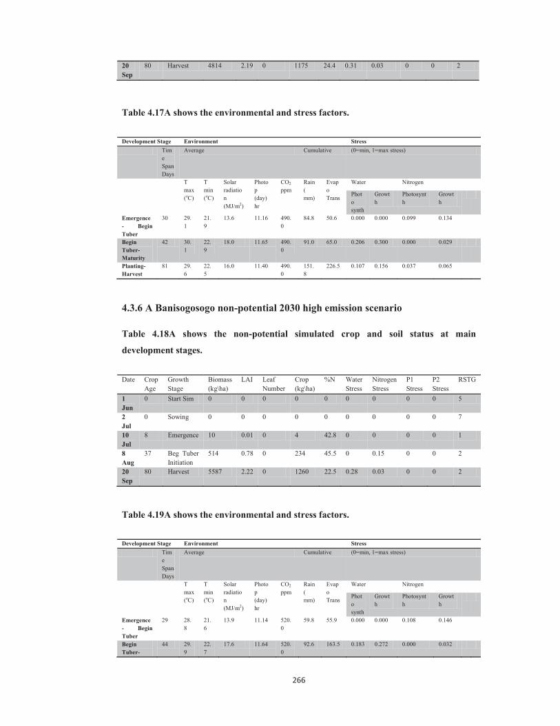
266
20 Sep
80 Harvest 4814 2.19 0 1175 24.4 0.31 0.03 0 0 2
Table 4.17A shows the environmental and stress factors.
Development Stage Environment Stress Tim
e Span Days
Average Cumulative (0=min, 1=max stress)
T max (oC)
T min (oC)
Solar radiation (MJ/m2)
Photop (day) hr
CO2 ppm
Rain ( mm)
Evapo Trans
Water Nitrogen
Photo synth
Growth
Photosynth
Growth
Emergence- Begin Tuber
30 29.1
21.9
13.6 11.16 490.0
84.8 50.6 0.000 0.000 0.099 0.134
Begin Tuber-Maturity
42 30.1
22.9
18.0 11.65 490.0
91.0 65.0 0.206 0.300 0.000 0.029
Planting-Harvest
81 29.6
22.5
16.0 11.40 490.0
151.8
226.5 0.107 0.156 0.037 0.065
4.3.6 A Banisogosogo non-potential 2030 high emission scenario
Table 4.18A shows the non-potential simulated crop and soil status at main
development stages.
Date Crop
Age Growth Stage
Biomass (kg\ha)
LAI Leaf Number
Crop (kg\ha)
%N Water Stress
Nitrogen Stress
P1 Stress
P2 Stress
RSTG
1 Jun
0 Start Sim 0 0 0 0 0 0 0 0 0 5
2 Jul
0 Sowing 0 0 0 0 0 0 0 0 0 7
10 Jul
8 Emergence 10 0.01 0 4 42.8 0 0 0 0 1
8 Aug
37 Beg Tuber Initiation
514 0.78 0 234 45.5 0 0.15 0 0 2
20 Sep
80 Harvest 5587 2.22 0 1260 22.5 0.28 0.03 0 0 2
Table 4.19A shows the environmental and stress factors.
Development Stage Environment Stress Tim
e Span Days
Average Cumulative (0=min, 1=max stress)
T max (oC)
T min (oC)
Solar radiation (MJ/m2)
Photop (day) hr
CO2 ppm
Rain ( mm)
Evapo Trans
Water Nitrogen
Photo synth
Growth
Photosynth
Growth
Emergence- Begin Tuber
29 28.8
21.6
13.9 11.14 520.0
59.8 55.9 0.000 0.000 0.108 0.146
Begin Tuber-
44 29.9
22.7
17.6 11.64 520.0
92.6 163.5 0.183 0.272 0.000 0.032
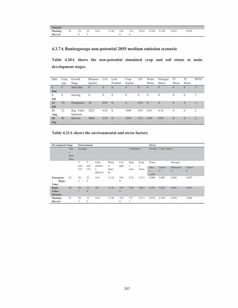
267
Maturity Planting-Harvest
81 29.4
22.3
16.0 11.40 520.0
154.4
229.0 0.100 0.148 0.039 0.070
4.3.7A Banisogosogo non-potential 2055 medium emission scenario
Table 4.20A shows the non-potential simulated crop and soil status at main
development stages.
Date Crop
Age Growth Stage
Biomass (kg\ha)
LAI Leaf Number
Crop (kg\ha)
%N Water Stress
Nitrogen Stress
P1 Stress
P2 Stress
RSTG
1 Jun
0 Start Sim 0 0 0 0 0 0 0 0 0 5
2 Jul
0 Sowing 0 0 0 0 0 0 0 0 0 7
12 Jul
10 Emergence 10 0.01 0 4 42.8 0 0 0 0 1
23 Aug
52 Beg Tuber Initiation
2632 4.01 0 1049 39.9 0.01 0.10 0 0 2
20 Sep
80 Harvest 4660 3.93 0 1545 33.2 0.30 0.05 0 0 2
Table 4.21A shows the environmental and stress factors.
Development Stage Environment Stress Tim
e Span Days
Average Cumulative (0=min, 1=max stress)
T max (oC)
T min (oC)
Solar radiation (MJ/m2)
Photop (day) hr
CO2 ppm
Rain ( mm)
Evapo Trans
Water Nitrogen
Photo synth
Growth
Photosynth
Growth
Emergence- Begin Tuber
42 30.2
22.9
14.6 11.24 550.0
97.0 113.3 0.000 0.006 0.069 0.097
Begin Tuber-Maturity
29 30.7
23.6
185 11.76 550.0
58.0 108.3 0.194 0.292 0.001 0.051
Planting-Harvest
81 30.3
23.2
16.0 11.40 550.0
157.1
233.3 0.070 0.108 0.036 0.069
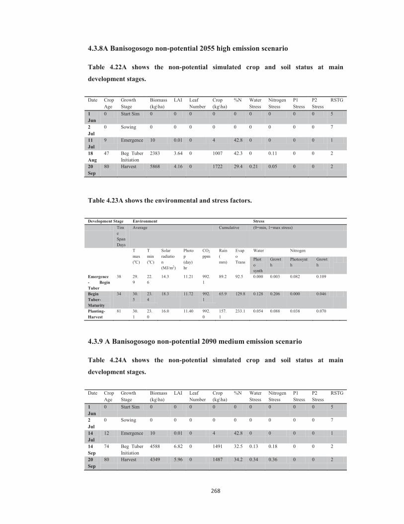
268
4.3.8A Banisogosogo non-potential 2055 high emission scenario
Table 4.22A shows the non-potential simulated crop and soil status at main
development stages.
Date Crop
Age Growth Stage
Biomass (kg\ha)
LAI Leaf Number
Crop (kg\ha)
%N Water Stress
Nitrogen Stress
P1 Stress
P2 Stress
RSTG
1 Jun
0 Start Sim 0 0 0 0 0 0 0 0 0 5
2 Jul
0 Sowing 0 0 0 0 0 0 0 0 0 7
11 Jul
9 Emergence 10 0.01 0 4 42.8 0 0 0 0 1
18 Aug
47 Beg Tuber Initiation
2383 3.64 0 1007 42.3 0 0.11 0 0 2
20 Sep
80 Harvest 5868 4.16 0 1722 29.4 0.21 0.05 0 0 2
Table 4.23A shows the environmental and stress factors.
Development Stage Environment Stress Tim
e Span Days
Average Cumulative (0=min, 1=max stress)
T max (oC)
T min (oC)
Solar radiation (MJ/m2)
Photop (day) hr
CO2 ppm
Rain ( mm)
Evapo Trans
Water Nitrogen
Photo synth
Growth
Photosynth
Growth
Emergence- Begin Tuber
38 29.9
22.6
14.3 11.21 992.1
89.2 92.5 0.000 0.003 0.082 0.109
Begin Tuber-Maturity
34 30.5
23.4
18.3 11.72 992.1
65.9 129.8 0.128 0.206 0.000 0.046
Planting-Harvest
81 30.1
23.0
16.0 11.40 992.0
157.1
233.1 0.054 0.088 0.038 0.070
4.3.9 A Banisogosogo non-potential 2090 medium emission scenario
Table 4.24A shows the non-potential simulated crop and soil status at main
development stages.
Date Crop
Age Growth Stage
Biomass (kg\ha)
LAI Leaf Number
Crop (kg\ha)
%N Water Stress
Nitrogen Stress
P1 Stress
P2 Stress
RSTG
1 Jun
0 Start Sim 0 0 0 0 0 0 0 0 0 5
2 Jul
0 Sowing 0 0 0 0 0 0 0 0 0 7
14 Jul
12 Emergence 10 0.01 0 4 42.8 0 0 0 0 1
14 Sep
74 Beg Tuber Initiation
4588 6.82 0 1491 32.5 0.13 0.18 0 0 2
20 Sep
80 Harvest 4349 5.96 0 1487 34.2 0.34 0.36 0 0 2

269
Table 4.25A shows the environmental and stress factors.
Development Stage Environment Stress Tim
e Span Days
Average Cumulative (0=min, 1=max stress)
T max (oC)
T min (oC)
Solar radiation (MJ/m2)
Photop (day) hr
CO2 ppm
Rain ( mm)
Evapo Trans
Water Nitrogen
Photo synth
Growth
Photosynth
Growth
Emergence- Begin Tuber
62 31.3
24.1
15.7 11.41 700.0
120.9
184.4 0.074 0.131 0.144 0.175
Begin Tuber-Maturity
7 32.5
25.4
21.5 11.94 700.0
28.1 29.4 0.244 0.292 0.337 0.370
Planting-Harvest
81 31.3
24.2
16.0 11.40 700.0
158.5
228.5 0.076 0.125 0.140 0.166
4.4A Optimisation treatment
4.4.1A Banisogosogo optimisation treatment
Table 4.26A shows the yield at different planting time for Banisogosogo under A1B and
A2 emission scenario.
Yield (kg/ha)
Planting Time
2030 A1B Emission
2030 A2 Emission
2055 A1B Emission
2055 A2 Emission
2090 A1B Emission
January 2 0 6 0 0 0
February 1 0 0 0 0 0
March 1 0 47 0 0 0
April 1 1442 1982 124 562 0
May 1 4684 5978 1906 3105 0
June 1 5004 6085 1933 2897 155
July 2 (default run)
4356 5158 2840 4015 597
August 1 4027 4744 1766 3039 125
September 1 871 1017 514 655 191
October 1 2004 2774 1480 2024 271
November 1 56 150 0 1 0
December 1 3 36 0 0 0

270
Table 4.27A shows the yield at different row spacing for Banisogosogo under A1B and
A2 emission scenario.
Yield (kg/ha)
Row Spacing ( cm)
Plant Population per m2
2030 A1B Emission
2030 A2 Emission
2055 A1B Emission
2055 A2 Emission
2090 A1B Emission
75 (default run)
5 2947 3703 1485 2566 17
30 11 2988 4081 1492 2464 18
40 8 2964 1005 1493 2479 18
50 6 2949 3793 1487 2555 17
80 4 2956 3697 1486 2599 17
100 3 2984 3711 1488 2603 10
Table 4.28A shows the yield under different irrigation amount for Banisogosogo under
A1B and A2 emission scenario.
Yield (kg/ha)
Default run (1.6 mm and 4.0 mm)
2947 3703 1485 2566 17
Irrigation ( mm)
2030 A1B Emission
2030 A2 Emission
2055 A1B Emission
2055 A2 Emission
2090 A1B Emission
1.6 4036 5060 1673 2656 20
4.0 4813 5784 1511 2587 12
6.4 5251 6465 1425 2275 3
8.0 4954 6189 1346 2163 1
9.6 4577 6087 1225 2041 1
12.0 4198 5838 1220 1986 1
14.4 3958 5447 1257 1959 1
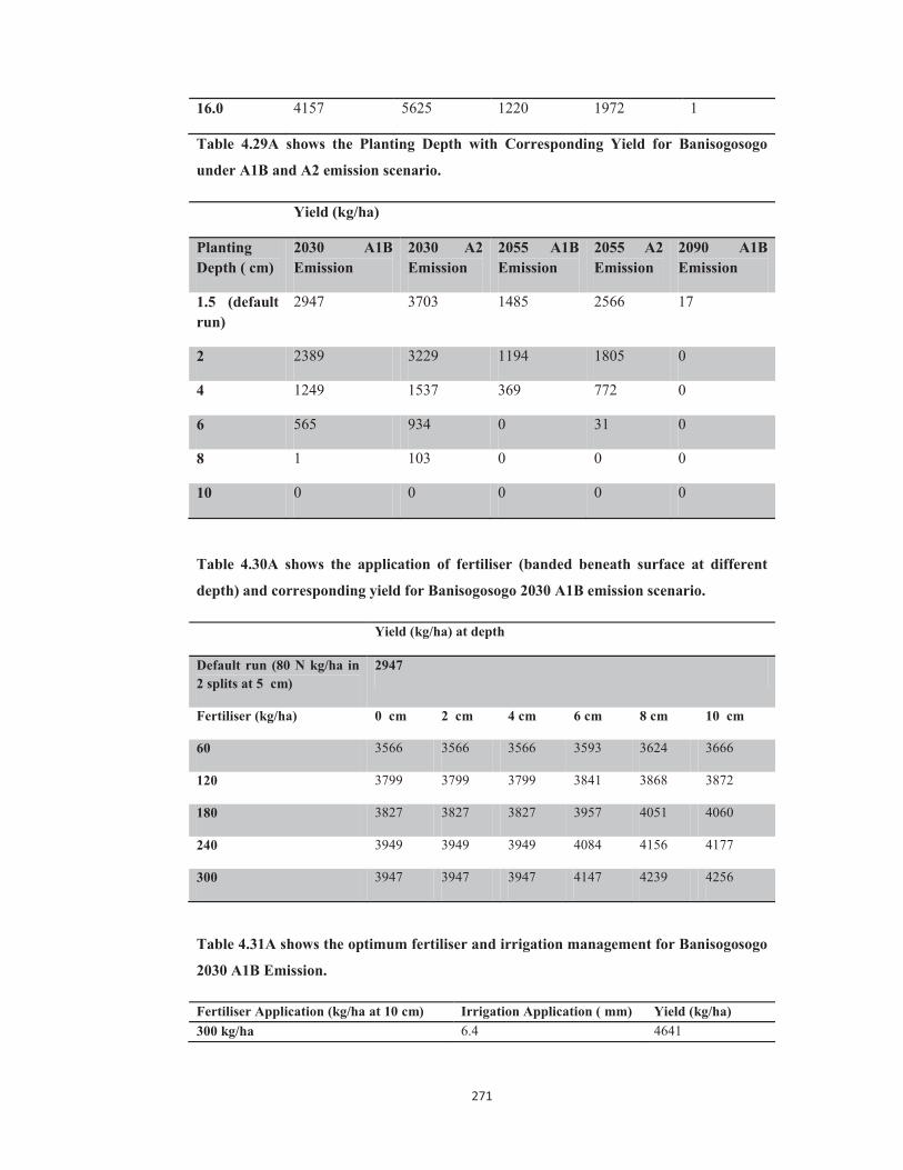
271
16.0 4157 5625 1220 1972 1
Table 4.29A shows the Planting Depth with Corresponding Yield for Banisogosogo
under A1B and A2 emission scenario.
Yield (kg/ha)
Planting Depth ( cm)
2030 A1B Emission
2030 A2 Emission
2055 A1B Emission
2055 A2 Emission
2090 A1B Emission
1.5 (default run)
2947 3703 1485 2566 17
2 2389 3229 1194 1805 0
4 1249 1537 369 772 0
6 565 934 0 31 0
8 1 103 0 0 0
10 0 0 0 0 0
Table 4.30A shows the application of fertiliser (banded beneath surface at different
depth) and corresponding yield for Banisogosogo 2030 A1B emission scenario.
Yield (kg/ha) at depth
Default run (80 N kg/ha in 2 splits at 5 cm)
2947
Fertiliser (kg/ha) 0 cm 2 cm 4 cm 6 cm 8 cm 10 cm
60 3566 3566 3566 3593 3624 3666
120 3799 3799 3799 3841 3868 3872
180 3827 3827 3827 3957 4051 4060
240 3949 3949 3949 4084 4156 4177
300 3947 3947 3947 4147 4239 4256
Table 4.31A shows the optimum fertiliser and irrigation management for Banisogosogo
2030 A1B Emission.
Fertiliser Application (kg/ha at 10 cm) Irrigation Application ( mm) Yield (kg/ha) 300 kg/ha 6.4 4641
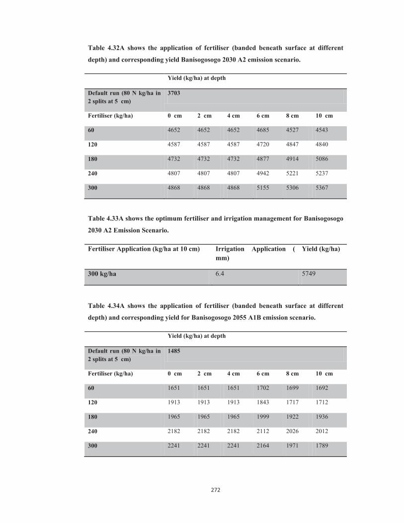
272
Table 4.32A shows the application of fertiliser (banded beneath surface at different
depth) and corresponding yield Banisogosogo 2030 A2 emission scenario.
Yield (kg/ha) at depth
Default run (80 N kg/ha in 2 splits at 5 cm)
3703
Fertiliser (kg/ha) 0 cm 2 cm 4 cm 6 cm 8 cm 10 cm
60 4652 4652 4652 4685 4527 4543
120 4587 4587 4587 4720 4847 4840
180 4732 4732 4732 4877 4914 5086
240 4807 4807 4807 4942 5221 5237
300 4868 4868 4868 5155 5306 5367
Table 4.33A shows the optimum fertiliser and irrigation management for Banisogosogo
2030 A2 Emission Scenario.
Fertiliser Application (kg/ha at 10 cm) Irrigation Application ( mm)
Yield (kg/ha)
300 kg/ha 6.4 5749
Table 4.34A shows the application of fertiliser (banded beneath surface at different
depth) and corresponding yield for Banisogosogo 2055 A1B emission scenario.
Yield (kg/ha) at depth
Default run (80 N kg/ha in 2 splits at 5 cm)
1485
Fertiliser (kg/ha) 0 cm 2 cm 4 cm 6 cm 8 cm 10 cm
60 1651 1651 1651 1702 1699 1692
120 1913 1913 1913 1843 1717 1712
180 1965 1965 1965 1999 1922 1936
240 2182 2182 2182 2112 2026 2012
300 2241 2241 2241 2164 1971 1789
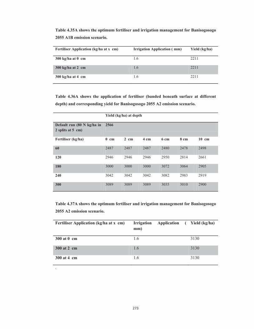
273
Table 4.35A shows the optimum fertiliser and irrigation management for Banisogosogo
2055 A1B emission scenario.
Fertiliser Application (kg/ha at x cm) Irrigation Application ( mm) Yield (kg/ha)
300 kg/ha at 0 cm 1.6 2211
300 kg/ha at 2 cm 1.6 2211
300 kg/ha at 4 cm 1.6 2211
Table 4.36A shows the application of fertiliser (banded beneath surface at different
depth) and corresponding yield for Banisogosogo 2055 A2 emission scenario.
Yield (kg/ha) at depth
Default run (80 N kg/ha in 2 splits at 5 cm)
2566
Fertiliser (kg/ha) 0 cm 2 cm 4 cm 6 cm 8 cm 10 cm
60 2487 2487 2487 2480 2478 2498
120 2946 2946 2946 2950 2814 2661
180 3000 3000 3000 3072 3064 2905
240 3042 3042 3042 3082 2983 2919
300 3089 3089 3089 3035 3010 2900
Table 4.37A shows the optimum fertiliser and irrigation management for Banisogosogo
2055 A2 emission scenario.
Fertiliser Application (kg/ha at x cm) Irrigation Application ( mm)
Yield (kg/ha)
300 at 0 cm 1.6 3130
300 at 2 cm 1.6 3130
300 at 4 cm 1.6 3130
.

274
Table 4.38A shows the application of fertiliser (banded beneath surface at different
depth) and corresponding yield for Banisogosogo 2090 A1B emission scenario.
Yield (kg/ha) at depth
Default run (80 N kg/ha in 2 splits at 5 cm)
17
Fertiliser (kg/ha) 0 cm 2 cm 4 cm 6 cm 8 cm 10 cm
60 38 38 38 29 29 29
120 19 19 19 20 20 20
180 11 11 11 11 12 12
240 10 10 10 10 11 11
300 5 5 5 6 5 5
Table 4.39A shows the optimum fertiliser and irrigation management for Banisogosogo
2090 A1B emission scenario.
Fertiliser Application (kg/ha at x cm) Irrigation Application ( mm)
Yield (kg/ha)
60 at 0 cm 1.6 991
60 at 2 cm 1.6 991
60 at 4 cm 1.6 991

275
4.5A Russet Burbank future climate simulation
4.5.1 A Banisogosogo non-potential 2030 high emission scenario
Table 4.40A shows the non-potential simulated crop and soil status at main
development stages.
Date Crop
Age Growth Stage
Biomass (kg\ha)
LAI Leaf Number
Crop (kg\ha)
%N Water Stress
Nitrogen Stress
P1 Stress
P2 Stress
RSTG
1 Jun
0 Start Sim 0 0 0 0 0 0 0 0 0 5
2 Jul
0 Sowing 0 0 0 0 0 0 0 0 0 7
10 Jul
8 Emergence 10 0.01 0 4 42.8 0 0 0 0 1
14 Sep
74 Beg Tuber Initiation
6153 8.96 0 1966 32.0 0.03 0.17 0 0 2
20 Sep
80 Harvest 5835 7.66 0 1967 33.7 0.18 0.38 0 0 2
Table 4.41A shows the environmental and stress factors.
Development Stage Environment Stress Tim
e Span Days
Average Cumulative (0=min, 1=max stress)
T max (oC)
T min (oC)
Solar radiation (MJ/m2)
Photop (day) hr
CO2 ppm
Rain ( mm)
Evapo Trans
Water Nitrogen
Photo synth
Growth
Photosynth
Growth
Emergence- Begin Tuber
66 29.3
22.2
15.5 11.39 520.0
84.8 125.0 0.005 0.029 0.133 0.163
Begin Tuber-Maturity
7 30.6
23.5
21.5 11.94 520.0
91.0 27.4 0.088 0.156 0.357 0.389
Planting-Harvest
81 29.4
22.3
16.0 11.40 520.0
151.8
154.4 0.011 0.037 0.139 0.167

276
4.6A Optimisation treatment
4.6.1A Banisogosogo optimisation treatment
Table 4.42A shows the yield at different planting time for Banisogosogo for Russet
Burbank variety for 2030 A2 emission scenario.
Yield (kg/ha)
Planting Time
2030 A1B Emission
2030 A2 Emission
2055 A1B Emission
2055 A2 Emission
2090 A1B Emission
2090 A2 Emission
January 2 0 0 0 0 0 0
February 1
0 0 0 0 0 0
March 1 0 0 0 0 0 0
April 1 0 0 0 0 0 0
May 1 0 0 0 0 0 0
June 1 22 165 0 0 0 0
July 2 (default run)
342 843 0 16 0 0
August 1 29 109 0 0 0 0
September 1
210 318 68 124 8 2
October 1 54 566 0 0 0 0
November 1
0 0 0 0 0 0
December 1
0 0 0 0 0 0

277
Table 4.43A shows the yield at different row spacing under 2030 A2 emission scenario
for Russet Burbank variety for Banisogosogo.
Yield (kg/ha)
Row Spacing ( cm)
Plant Population per m2
2030 A1B Emission
2030 A2 Emission
2055 A1B Emission
2055 A2 Emission
2090 A1B Emission
2090 A2 Emission
75 (default run)
5 0 37 0 0 0 0
30 11 1 38 1 1 1 1
40 8 1 38 1 1 1 1
50 6 1 37 1 1 1 1
80 4 0 36 0 0 0 0
100 3 0 22 0 0 0 0
Table 4.44A shows the yield under different irrigation application and irrigation
amount for Russet Burbank for Banisogosogo under 2030 A2 emission scenario.
Yield (kg/ha)
Default run (1.6 mm and 4.0 mm)
0 37 0 0 0 0
Irrigation ( mm) 2030 A1B Emission
2030 A2 Emission
2055 A1B Emission
2055 A2 Emission
2090 A1B Emission
2090 A2 Emission
1.6 1 88 0 0 0 0
4.0 0 50 0 0 0 0
6.4 0 30 0 0 0 0
8.0 0 18 0 0 0 0
9.6 0 18 0 0 0 0
12.0 0 31 0 0 0 0
14.4 0 31 0 0 0 0
16.0 0 31 0 0 0 0

278
Table 4.45A shows the planting depth with corresponding yield for Russet Burbank for
Banisogosogo under 2030 A2 emission scenario.
Yield (kg/ha)
Planting Depth ( cm)
2030 A1B Emission
2030 A2 Emission
2055 A1B Emission
2055 A2 Emission
2090 A1B Emission
2090 A2 Emission
1.5 (default run)
0 37 0 0 0 0
2 0 12 0 0 0 0
4 0 0 0 0 0 0
6 0 0 0 0 0 0
8 0 0 0 0 0 0
10 0 0 0 0 0 0
Table 4.46A shows the application of fertiliser (banded beneath surface at different
depth) and corresponding yield for Banisogosogo under 2030 A1B emission.
Yield (kg/ha) at depth
Default run (80 N kg/ha in 2 splits at 5 cm)
0
Fertiliser (kg/ha) 0 cm 2 cm 4 cm 6 cm 8 cm 10 cm
60 7 7 7 7 7 7
120 3 3 3 3 3 3
180 1 1 1 1 1 1
240 0 0 0 0 0 0
300 0 0 0 0 0 0

279
Table 4.47A shows the optimum fertiliser and irrigation management for Koronivia
under 2030 A1B emission.
Optimum Fertiliser and Irrigation Management
Fertiliser Application (kg/ha at x cm) Irrigation Application ( mm) Yield (kg/ha)
60 kg/ha at 0-8 cm 1.6 6
60 kg/ha at 10 cm 1.6 7
Table 4.48A shows the application of fertiliser (banded beneath surface at different
depth) and corresponding yield for Banisogogsogo under 2030 A2emission.
Yield (kg/ha) at depth
Default run (80 N kg/ha in 2 splits at 5 cm)
37
Fertiliser (kg/ha) 0 cm 2 cm 4 cm 6 cm 8 cm 10 cm
60 150 150 150 151 151 151
120 104 104 104 104 104 87
180 85 85 85 85 48 48
240 46 46 46 29 16 16
300 15 15 15 7 4 2
Table 4.49A shows the optimum fertiliser and irrigation management for Banisogosogo
under 2030 A1B emission.
Optimum Fertiliser and Irrigation Management
Fertiliser Application (kg/ha at x cm) Irrigation Application ( mm) Yield (kg/ha)
60 kg/ha at 6 cm 1.6 151
60 kg/ha at 8 cm 1.6 151
60 kg/ha at 10 cm 1.6 151


