

Evaluating the macroeconomic effects of the ECB’s unconventional
monetary policies Sarah Mouabbi1 and Jean-Guillaume Sahuc2
February 2019, WP #708
ABSTRACT We quantify the macroeconomic effects of the European Central Bank’s unconventional monetary policies using a DSGE model which includes a set of shadow interest rates. Extracted from the yield curve, these shadow rates provide unconstrained measures of the overall stance of monetary policy. Counterfactual analyses show that, without unconventional measures, the euro area would have suffered (i) a substantial loss of output since the Great Recession and (ii) a period of deflation from mid-2015 to early 2017. Specifically, year-on-year inflation and GDP growth would have been on average about 0.61% and 1.09% below their actual levels over the period 2014Q1-2017Q2, respectively.
Keywords: Unconventional monetary policy, shadow policy rate, DSGE model, euro area
JEL classification: E32 ; E44 ; E52
1 Banque de France, Financial Economics Research Division, [email protected] ; 2 Banque de France, Financial Economics Research Division, and University Paris-Nanterre, [email protected] ; We are grateful to the editor, Kenneth West, two anonymous referees, as well as Boragan Aruoba, Régis Barnichon, Jonathan Benchimol, Efrem Castelnuovo, Marco Del Negro, Jordi Gali, Arne Halberstadt, Eric Jondeau, Michel Juillard, Leo Krippner, Michael Kuhl, Mariano Kulish, Thomas Laubach, Julien Matheron, Claudio Michelacci, Benoit Mojon, Luca Onorante, Athanasios Orphanides, Christian Pfister, Dominic Quint, Ricardo Reis, Barbara Rossi, Glenn Rudebusch, Frank Schorfheide, Frank Smets, Carlos Thomas, Harald Uhlig, Raf Wouters, Cynthia Wu, Francesco Zanetti, and the participants of several conferences for their useful comments and suggestions. We also thank Tomi Kortela, Wolfgang Lemke and Andreea Vladu for providing us with their series. The views expressed in this paper are those of the authors and do not necessarily reflect the views of the Banque de France or the Eurosystem.
Working Papers reflect the opinions of the authors and do not necessarily express the views of the Banque de France. This document is available on publications.banque-france.fr/en
Banque de France WP #708 ii
NON-TECHNICAL SUMMARY
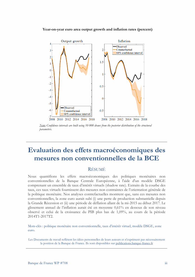
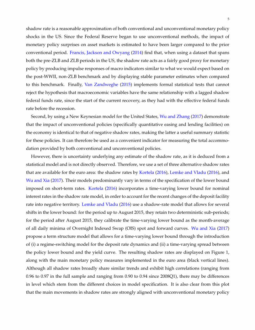
Decisions of central banks rely on an assessment of their monetary policy stance, i.e. the contribution made by monetary policy to real economic and financial developments. In the past, policymakers could compare the policy rate to the prescriptions of simple policy rules, to get a sense of whether their actions were appropriate in view of their objectives. However, the severity of the financial crisis in 2008 led many central banks to lower their key rates at levels close to their effective lower bound (ELB), limiting their ability to stimulate further the economy. Unable to move the short-end of the yield curve, central banks turned to a number of unconventional policies to provide additional monetary accommodation. In the context of the euro area, these policies included an increase in the average maturity of outstanding liquidity, the use of forward guidance, several asset purchase programs and negative deposit facility rates. With the implementation of such measures, there is no directly observable indicator that summarizes the stance of policy. How can one quantify the effects of these new policy measures from a macroeconomic perspective? In this paper, we address this question by integrating a set of shadow policy rates in a dynamic stochastic general equilibrium (DSGE) model to reveal the macroeconomic effects of unconventional measures implemented by the European Central Bank (ECB). The shadow rate is the shortest maturity rate, extracted from a term structure model, that would generate the observed yield curve had the ELB not been binding. It incorporates both the effect of monetary policy measures on current economic conditions as well as market expectations of future policy actions. The shadow rate coincides with the policy rate in normal times and is free to go into negative territory when the policy rate is stuck at its lower bound. Particularly, exploiting the entire yield curve allows to account for the influence of direct and/or indirect market interventions on intermediate and longer maturity rates. It can therefore be used as a convenient indicator for measuring the total accommodation provided by both conventional and unconventional policies. Therefore, we propose to compare a Taylor rule based on the common component extracted from a set of shadow rates with the Eonia rate. Taking the common component allows us to address the uncertainty surrounding the measurement of shadow rates. The resulting shadow rate is then used to extract the shocks stemming from all monetary policy actions within our DSGE model. Through a counterfactual exercise, these shocks can subsequently be replaced by shocks that would have kept the shadow rate at the Eonia rate level, i.e the rate that represents the conventional part of monetary policy. This analysis enables us to isolate and gauge the effects of unconventional policies on economic activity and inflation. We find that in the absence of such monetary policies, the euro area would have suffered a quarterly output loss of about 4.5% in 2017Q2. Moreover, these measures helped in avoiding a period of deflation from mid-2015 to early 2017. This translates into year-on-year (y-o-y) inflation and GDP growth differentials of 0.26% and 0.51% on average over the period 2008Q1-2017Q2, respectively. Drawing attention on the period 2014Q1- 2017Q2, when public and private sector asset purchase programs have been announced and conducted, y-o-y inflation and GDP growth would have been lower by 0.61% and 1.09%, respectively (see figure below). Our approach has the advantage of overcoming the computational issues associated with the presence of the ELB by using traditional estimation techniques.
Banque de France WP #708 iii
Year-on-year euro area output growth and inflation rates (percent)
Note: Confidence intervals are built using 10 000 draws from the posterior distribution of the structural parameters.
Evaluation des effets macroéconomiques des mesures non conventionnelles de la BCE
RÉSUMÉ Nous quantifions les effets macroéconomiques des politiques monétaires non conventionnelles de la Banque Centrale Européenne, à l'aide d'un modèle DSGE comprenant un ensemble de taux d’intérêt virtuels (shadow rate). Extraits de la courbe des taux, ces taux virtuels fournissent des mesures non contraintes de l’orientation générale de la politique monétaire. Nos analyses contrefactuelles montrent que, sans ces mesures non conventionnelles, la zone euro aurait subi (i) une perte de production substantielle depuis la Grande Récession et (ii) une période de déflation allant de la mi-2015 au début 2017. Le glissement annuel de l’inflation aurait été en moyenne 0,61% en dessous de son niveau observé et celui de la croissance du PIB plus bas de 1,09%, au cours de la période 2014T1-2017T2. Mots-clés : politique monétaire non conventionnelle, taux d’intérêt virtuel, modèle DSGE, zone euro. Les Documents de travail reflètent les idées personnelles de leurs auteurs et n'expriment pas nécessairement
la position de la Banque de France. Ils sont disponibles sur publications.banque-france.fr
1. INTRODUCTION
Decisions of central banks rely on an assessment of their monetary policy stance, i.e. the contribu-
tion made by monetary policy to real economic and financial developments. In the past, policymakers
could compare the policy rate to the prescriptions of simple policy rules, to get a sense of whether
their actions were appropriate in view of their objectives. However, the severity of the financial crisis
in 2008 led many central banks to lower their key rates at levels close to their effective lower bound
(ELB), limiting their ability to stimulate further the economy. Unable to move the short-end of the
yield curve, central banks turned to a number of unconventional policies to provide additional mone-
tary accommodation. In the context of the euro area, these policies included an increase in the average
maturity of outstanding liquidity, the use of forward guidance, several asset purchase programs and
negative deposit facility rates. With the implementation of such measures, there is no directly observ-
able indicator that summarizes the stance of policy. How can one quantify the effects of these new
policy measures from a macroeconomic perspective?
In this paper, we address this question by integrating a set of shadow policy rates in a dynamic
stochastic general equilibrium (DSGE) model to reveal the macroeconomic effects of unconventional
measures implemented by the European Central Bank (ECB).
The shadow rate is the shortest maturity rate, extracted from a term structure model, that would
generate the observed yield curve had the ELB not been binding (Kim and Singleton, 2012; Kripp-
ner, 2012; Christensen and Rudebusch, 2015, 2016). It incorporates both the effect of monetary policy
measures on current economic conditions as well as market expectations of future policy actions. The
shadow rate coincides with the policy rate in normal times and is free to go into negative territory
when the policy rate is stuck at its lower bound. Claus, Claus and Krippner (2014), Francis, Jack-
son and Owyang (2014) and Van Zandweghe (2015) show that the shadow rate captures the stance
of monetary policy during lower bound episodes in the same way the policy rate does in normal
times. Hence, the dynamic relationships between macroeconomic variables and monetary policy are
preserved, in any economic environment, by using a shadow rate. Particularly, exploiting the entire
yield curve allows to account for the influence of direct and/or indirect market interventions on inter-
mediate and longer maturity rates. It can therefore be used as a convenient indicator for measuring
the total accommodation provided by both conventional and unconventional policies (Krippner, 2013;
Wu and Xia, 2016).
In order to adequately quantify the macroeconomic effects of unconventional policies, we further
need a macroeconomic model that is structural in the sense that: (i) it formalizes the behavior of
economic agents on the basis of explicit micro-foundations and (ii) it can appropriately control for
the effects of policy measures through expectations to respond to the Lucas (1976) critique. Hence,
1
2
we consider a medium-scale DSGE model à la Smets and Wouters (2007), as it has been successful
in providing an empirically plausible account of key macroeconomic variables (see also Christiano
et al., 2017, for a discussion on the importance of DSGE models in the policy process). We deliberately
choose to keep such a standard framework because: (i) it is challenging to incorporate all the channels
through which we think unconventional measures can act (selecting only a few of these channels
could distort the results) and (ii) introducing a shadow rate in a model has the advantage of by-
passing the non-linearity stemming from the existence of the lower bound. In addition, Wu and Zhang
(2017) theoretically show that the impact of unconventional measures (particularly asset purchases
and lending facilities) is identical to that of a negative shadow rate that enters directly into the IS
curve, validating our approach.
Therefore, we propose to compare a Taylor rule based on the common component extracted from
a set of shadow rates with the Eonia rate. Taking the common component allows us to address the
uncertainty surrounding the measurement of shadow rates. The resulting shadow rate is then used
to extract the shocks stemming from all monetary policy actions within our DSGE model. Through
a counterfactual exercise, these shocks can subsequently be replaced by shocks that would have kept
the shadow rate at the Eonia rate level, i.e the rate that represents the conventional part of monetary
policy. This analysis enables us to isolate and gauge the effects of unconventional policies on economic
activity and inflation.
We find that in the absence of such monetary policies, the euro area would have suffered a quarterly
output loss of about 4.5% in 2017Q2. Moreover, these measures helped in avoiding a period of defla-
tion from mid-2015 to early 2017. This translates into year-on-year (y-o-y) inflation and GDP growth
differentials of 0.26% and 0.51% on average over the period 2008Q1-2017Q2, respectively. Drawing at-
tention on the period 2014Q1-2017Q2, when public and private sector asset purchase programs have
been announced and conducted, y-o-y inflation and GDP growth would have been lower by 0.61% and
1.09%, respectively. Our analysis also highlights that we can still use standard linear DSGE models
in low interest rate environments when using an unconstrained proxy of the monetary policy stance
such as the shadow rate.
Despite the growing interest in unconventional monetary policies, the literature has mainly concen-
trated on the effects of FOMC-decisions on financial markets, especially through event studies (see the
survey by Bhattarai and Neely, 2016). There are relatively few studies that investigate the impact of
unconventional monetary policies on macro variables, whether for the United States or the euro area.1
1These studies include Chen, Cúrdia and Ferrero (2012), Baumeister and Benati (2013), Gertler and Karadi (2013),Cova, Pagano and Pisani (2015), Andrade, Breckenfelder, De Fiore, Karadi and Tristani (2016), Sahuc (2016) and Wealeand Wieladek (2016) on asset purchases, Del Negro, Eggertsson, Ferrero and Kiyotaki (2017) and Cahn, Matheron and Sahuc(2017) on liquidity injections, and Del Negro, Giannoni and Patterson (2015), McKay, Nakamura and Steinsson (2016), Sahuc(2016) and Kulish, Morley and Robinson (2017) on forward guidance.
3
In addition, these studies focus exclusively on the effects of a subset of unconventional monetary mea-
sures (i.e. they study asset purchases, liquidity injections, or forward guidance in isolation), with the
notable exceptions of Engen, Laubach and Reifschneider (2015) and Wu and Xia (2016). The former
evaluate the macroeconomic effects of both forward guidance and asset purchases in the United States
by including private-sector forecasters’ perceptions of monetary policy in a DSGE model. Nonethe-
less, survey data are not available at a sufficiently high frequency making the stance of monetary
policy harder to gauge in real time. The latter assess the effects of the various measures adopted by
the Fed after the Great Recession using their estimate of the shadow rate in a factor-augmented Vector
Autoregression (VAR). However, VAR-based policy counterfactuals are sensitive to (i) unknown struc-
tural characteristics of the underlying data generating process and (ii) identification schemes (Benati,
2010). Note that the VAR model by Wu and Xia (2016) displays a price puzzle (i.e. aggregate prices
and the interest rate move in the same direction following a monetary policy shock) that can cause
difficulties in interpretation when considering counterfactual monetary policy regimes.
Our paper is the first to introduce shadow rates within a consistent DSGE framework to provide
a tractable assessment of the macroeconomic effects of all unconventional policies implemented by
a central bank since 2008. Our approach has the advantage of overcoming the computational issues
associated with the presence of the ELB by using traditional estimation techniques.
In the remainder of the paper Section 2 introduces shadow policy rates for the euro area, Section 3
describes the dynamic stochastic general equilibrium model and its estimation, Section 4 presents our
empirical results on the quantification of the effects of unconventional monetary policy measures in
the euro area, and Section 5 concludes.
2. SHADOW INTEREST RATES AND MONETARY POLICY
Shadow rates have become increasingly popular in summarizing the stance of monetary policy due
to their maintained correlation with macroeconomic variables, even when key policy rates are kept
at the ELB (see, Krippner, 2013; Hakkio and Kahn, 2014; Doh and Choi, 2016; Wu and Xia, 2016).
This desirable property comes from the fact that shadow rates typically stem from term structure
models which exploit the entire yield curve, including long-term yields which are highly informative
on expectations of future short-term yields. Particularly, the shadow rate is the shortest maturity
rate, extracted from a term structure model, that would generate the observed yield curve had the
ELB not been binding (Kim and Singleton, 2012; Krippner, 2012; Christensen and Rudebusch, 2015,
2016).2 The shadow rate coincides with the policy rate in normal times and is free to go into negative
2Shadow-rate term structure models account for the ELB by setting the policy rate Rt, which is used for discounting cashflows when valuing securities, equal to the lower bound bt or the shadow rate St, whichever is larger: Rt = max (bt, St).Therefore, within the confines of shadow-rate term structure models, the shadow rate St is (by construction) the short-rate that explains the yield curve in a fictitious world where the ELB is not binding. This is also why the shadow rate Stcoincindes with the policy rate Rt in periods when the ELB is not binding.
4
territory when the policy rate is stuck at its lower bound. Specifically, exploiting the entire yield curve
allows to account for the influence of direct and/or indirect market interventions on intermediate
and longer maturity rates. Therefore, it incorporates both the effect of monetary policy measures on
current economic conditions as well as market expectations of future policy actions.The shadow policy
rate can then be easily plugged into existing quantitative models for monetary policy analysis.
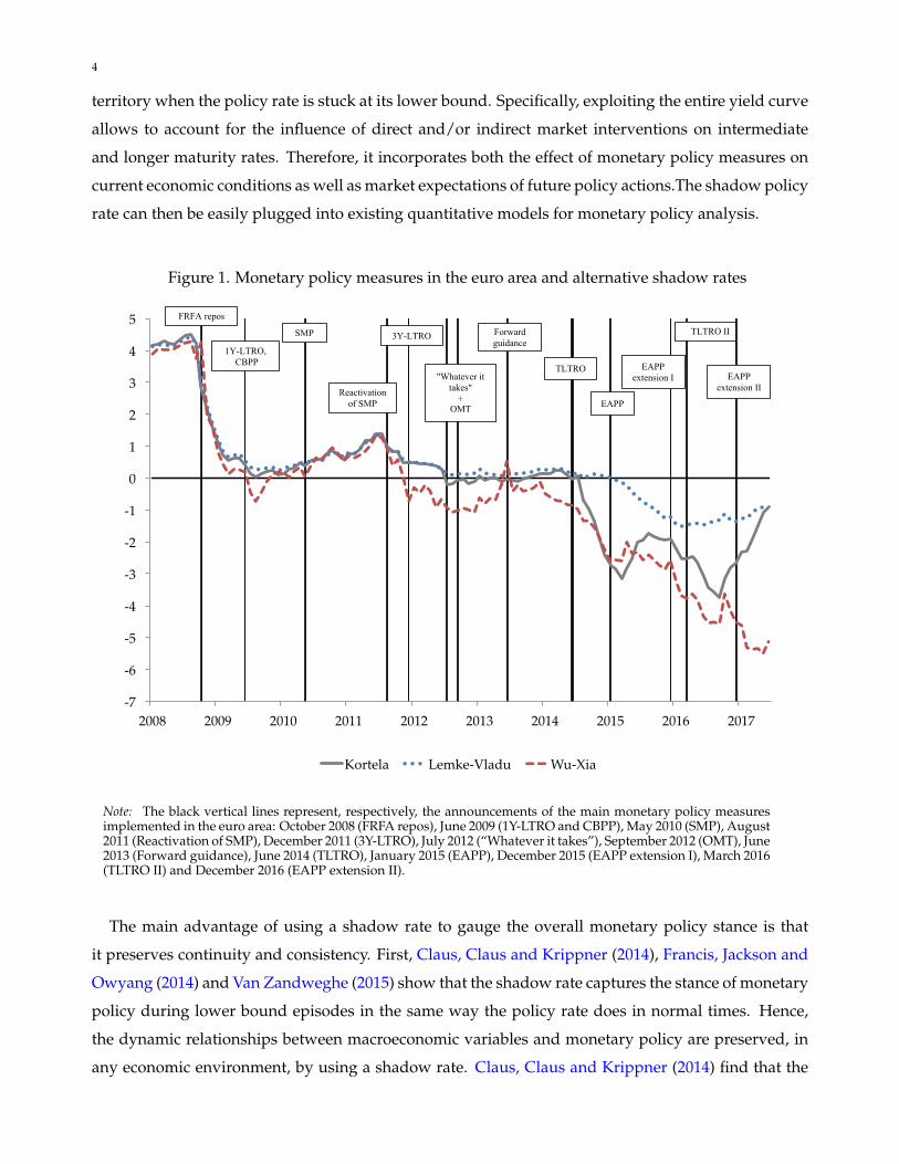
Figure 1. Monetary policy measures in the euro area and alternative shadow rates
-7
-6
-5
-4
-3
-2
-1
0
1
2
3
4
5
2008 2009 2010 2011 2012 2013 2014 2015 2016 2017
Kortela Lemke-Vladu Wu-Xia
Reactivationof SMP
FRFA repos
1Y-LTRO,CBPP
SMP 3Y-LTRO
"Whatever it takes"
+OMT
Forward guidance
TLTRO
EAPP
EAPPextension I
TLTRO II
EAPPextension II
Note: The black vertical lines represent, respectively, the announcements of the main monetary policy measuresimplemented in the euro area: October 2008 (FRFA repos), June 2009 (1Y-LTRO and CBPP), May 2010 (SMP), August2011 (Reactivation of SMP), December 2011 (3Y-LTRO), July 2012 (“Whatever it takes”), September 2012 (OMT), June2013 (Forward guidance), June 2014 (TLTRO), January 2015 (EAPP), December 2015 (EAPP extension I), March 2016(TLTRO II) and December 2016 (EAPP extension II).
The main advantage of using a shadow rate to gauge the overall monetary policy stance is that
it preserves continuity and consistency. First, Claus, Claus and Krippner (2014), Francis, Jackson and
Owyang (2014) and Van Zandweghe (2015) show that the shadow rate captures the stance of monetary
policy during lower bound episodes in the same way the policy rate does in normal times. Hence,
the dynamic relationships between macroeconomic variables and monetary policy are preserved, in
any economic environment, by using a shadow rate. Claus, Claus and Krippner (2014) find that the
5
shadow rate is a reasonable approximation of both conventional and unconventional monetary policy
shocks in the US. Since the Federal Reserve began to use unconventional methods, the impact of
monetary policy surprises on asset markets is estimated to have been larger compared to the prior
conventional period. Francis, Jackson and Owyang (2014) find that, when using a dataset that spans
both the pre-ZLB and ZLB periods in the US, the shadow rate acts as a fairly good proxy for monetary
policy by producing impulse responses of macro indicators similar to what we would expect based on
the post-WWII, non-ZLB benchmark and by displaying stable parameter estimates when compared
to this benchmark. Finally, Van Zandweghe (2015) implements formal statistical tests that cannot
reject the hypothesis that macroeconomic variables have the same relationship with a lagged shadow
federal funds rate, since the start of the current recovery, as they had with the effective federal funds
rate before the recession.
Second, by using a New Keynesian model for the United States, Wu and Zhang (2017) demonstrate
that the impact of unconventional policies (specifically quantitative easing and lending facilities) on
the economy is identical to that of negative shadow rates, making the latter a useful summary statistic
for these policies. It can therefore be used as a convenient indicator for measuring the total accommo-
dation provided by both conventional and unconventional policies.
However, there is uncertainty underlying any estimate of the shadow rate, as it is deduced from a
statistical model and is not directly observed. Therefore, we use a set of three alternative shadow rates
that are available for the euro area: the shadow rates by Kortela (2016), Lemke and Vladu (2016), and
Wu and Xia (2017). Their models predominantly vary in terms of the specification of the lower bound
imposed on short-term rates. Kortela (2016) incorporates a time-varying lower bound for nominal
interest rates in the shadow rate model, in order to account for the recent changes of the deposit facility
rate into negative territory. Lemke and Vladu (2016) use a shadow-rate model that allows for several
shifts in the lower bound: for the period up to August 2015, they retain two deterministic sub-periods;
for the period after August 2015, they calibrate the time-varying lower bound as the month-average
of all daily minima of Overnight Indexed Swap (OIS) spot and forward curves. Wu and Xia (2017)
propose a term structure model that allows for a time-varying lower bound through the introduction
of (i) a regime-switching model for the deposit rate dynamics and (ii) a time-varying spread between
the policy lower bound and the yield curve. The resulting shadow rates are displayed on Figure 1,
along with the main monetary policy measures implemented in the euro area (black vertical lines).
Although all shadow rates broadly share similar trends and exhibit high correlations (ranging from
0.96 to 0.97 in the full sample and ranging from 0.90 to 0.94 since 2008Q1), there may be differences
in level which stem from the different choices in model specification. It is also clear from this plot
that the main movements in shadow rates are strongly aligned with unconventional monetary policy

6
announcements. For instance, the TLTRO announcement in 2014 is followed by the sharpest drop in
shadow rates on average.
In order to account for measurement uncertainty, we extract one common factor from the set of the
three alternative shadow rates. Our objective is to identify the factor that explains the commonalities
between the three alternative measures, such that if the factor is held constant, the partial correlations
among the alternative measures are all equal to zero. Therefore, the latent common factor is a driver
of the three observed measures. In our analysis, we directly introduce all three alternative measures
in the structural model to endogenously extract their common factor, which we ultimately use as the
representative shadow rate.
3. ESTIMATING A MACROECONOMIC MODEL USING SHADOW RATES
This section presents the structural model used for quantifying the macroeconomic effects of un-
conventional policies, and discusses the estimation results on the 1999Q1-2017Q2 period.
3.1. The structural model. The model combines a neoclassical growth core with several shocks and
frictions (see Smets and Wouters, 2007; Justiniano et al., 2010). It includes features such as habit forma-
tion, investment adjustment costs, variable capital utilization, monopolistic competition in goods and
labor markets, and nominal price and wage rigidities. The economy is populated by five classes of
agents: producers of a final good, intermediate goods’ producers, households, employment agencies
and the public sector (government and monetary authorities).3 The nominal interest rate is assumed to
be the representative shadow rate, obtained as a common factor of the three alternative shadow rates.
Obviously, no transactions are taking place at the shadow rate, but various borrowing/lending rates
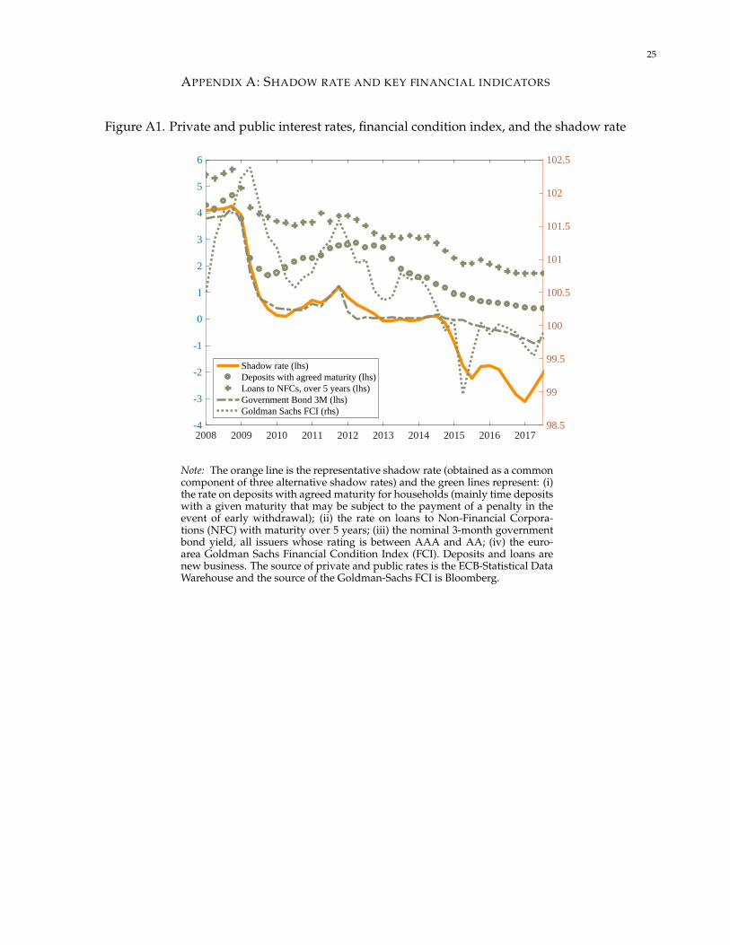
that private agents face co-move with it, with correlations of about 0.9 (see Figure A1 of Appendix A).
This strong link between bank rates and the shadow rate has also been documented by Wu and Zhang
(2017) in the case of the United States. This indicates that the shadow rate has comparable dynamics
to the borrowing/lending rates (notably to the 3-month government bond rate, the underlying coun-
terpart in the model, which becomes negative from mid-2014) and that the difference in levels results
from the additional easing of financing conditions provided by the non-standard measures.
3.1.1. Household sector.
Employment agencies–. Each household indexed by j ∈ [0, 1] is a monopolistic supplier of specialized
labor Nj,t. At every point in time t, a large number of competitive “employment agencies” com-
bine households’ labor into a homogenous labor input Nt sold to intermediate firms, according to
Nt =
[∫ 10 Nj,t
1εw,t dj
]εw,t
. Profit maximization by the perfectly competitive employment agencies im-
plies the labor demand function Nj,t =(
Wj,tWt
)− εw,tεw,t−1 Nt, where Wj,t is the wage paid by employment
3In the following, we let variables without a time subscript denote steady-state values.
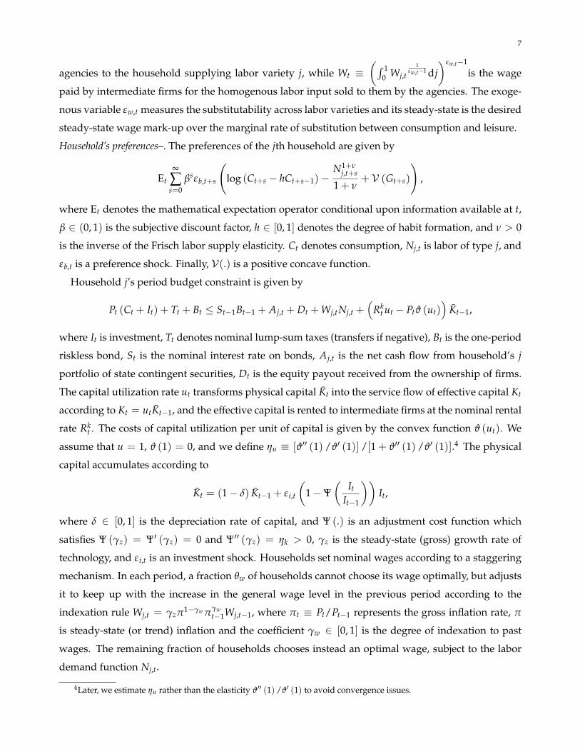
7
agencies to the household supplying labor variety j, while Wt ≡(∫ 1
0 Wj,t1
εw,t−1 dj)εw,t−1
is the wage
paid by intermediate firms for the homogenous labor input sold to them by the agencies. The exoge-
nous variable εw,t measures the substitutability across labor varieties and its steady-state is the desired
steady-state wage mark-up over the marginal rate of substitution between consumption and leisure.
Household’s preferences–. The preferences of the jth household are given by
Et
∞
∑s=0
βsεb,t+s
(log (Ct+s − hCt+s−1)−
N1+νj,t+s
1 + ν+ V (Gt+s)
),
where Et denotes the mathematical expectation operator conditional upon information available at t,
β ∈ (0, 1) is the subjective discount factor, h ∈ [0, 1] denotes the degree of habit formation, and ν > 0
is the inverse of the Frisch labor supply elasticity. Ct denotes consumption, Nj,t is labor of type j, and
εb,t is a preference shock. Finally, V(.) is a positive concave function.
Household j’s period budget constraint is given by
Pt (Ct + It) + Tt + Bt ≤ St−1Bt−1 + Aj,t + Dt + Wj,tNj,t +(
Rkt ut − Ptϑ (ut)
)Kt−1,
where It is investment, Tt denotes nominal lump-sum taxes (transfers if negative), Bt is the one-period
riskless bond, St is the nominal interest rate on bonds, Aj,t is the net cash flow from household’s j
portfolio of state contingent securities, Dt is the equity payout received from the ownership of firms.
The capital utilization rate ut transforms physical capital Kt into the service flow of effective capital Kt
according to Kt = utKt−1, and the effective capital is rented to intermediate firms at the nominal rental
rate Rkt . The costs of capital utilization per unit of capital is given by the convex function ϑ (ut). We
assume that u = 1, ϑ (1) = 0, and we define ηu ≡ [ϑ′′ (1) /ϑ′ (1)] /[1 + ϑ′′ (1) /ϑ′ (1)].4 The physical
capital accumulates according to
Kt = (1− δ) Kt−1 + ε i,t
(1−Ψ
(It
It−1
))It,
where δ ∈ [0, 1] is the depreciation rate of capital, and Ψ (.) is an adjustment cost function which
satisfies Ψ (γz) = Ψ′ (γz) = 0 and Ψ′′ (γz) = ηk > 0, γz is the steady-state (gross) growth rate of
technology, and ε i,t is an investment shock. Households set nominal wages according to a staggering
mechanism. In each period, a fraction θw of households cannot choose its wage optimally, but adjusts
it to keep up with the increase in the general wage level in the previous period according to the
indexation rule Wj,t = γzπ1−γw πγwt−1Wj,t−1, where πt ≡ Pt/Pt−1 represents the gross inflation rate, π
is steady-state (or trend) inflation and the coefficient γw ∈ [0, 1] is the degree of indexation to past
wages. The remaining fraction of households chooses instead an optimal wage, subject to the labor
demand function Nj,t.
4Later, we estimate ηu rather than the elasticity ϑ′′ (1) /ϑ′ (1) to avoid convergence issues.
8
3.1.2. Business sector.
Final good producers–. At every point in time t, a perfectly competitive sector produces a final good Yt
by combining a continuum of intermediate goods Yt (ς), ς ∈ [0, 1], according to the technology Yt =[∫ 10 Yς,t
1ε p,t dς
]εp,t
. Final good producing firms take their output price, Pt, and their input prices, Pς,t,
as given and beyond their control. Profit maximization implies Yς,t =(
Pς,tPt
)− ε p,tε p,t−1 Yt from which we
deduce the relationship between the price of the final good and the prices of intermediate goods Pt ≡[∫ 10 Pς,t
1εp,t−1 dς
]εp,t−1
. The exogenous variable εp,t measures the substitutability across differentiated
intermediate goods and its steady state is then the desired steady-state price markup over the marginal
cost of intermediate firms.
Intermediate-goods firms–. Intermediate good ς is produced by a monopolistic firm using the following
production function
Yς,t = Kς,tα [ZtNς,t]
1−α − ZtΩ,
where α ∈ (0, 1) denotes the capital share, Kς,t and Nς,t denote the amounts of capital and effective
labor used by firm ς, Ω is a fixed cost of production that ensures that profits are zero in steady state,
and Zt is an exogenous labor-augmenting productivity factor whose growth-rate is denoted by εz,t ≡Zt/Zt−1. In addition, we assume that intermediate firms rent capital and labor in perfectly competitive
factor markets.
Intermediate firms set prices according to a staggering mechanism. In each period, a fraction θp
of firms cannot choose its price optimally, but adjusts it to keep up with the increase in the general
price level in the previous period according to the indexation rule Pς,t = π1−γp πγpt−1Pς,t−1,where the
coefficient γp ∈ [0, 1] indicates the degree of indexation to past prices. The remaining fraction of firms
chooses its price P?ς,t optimally, by maximizing the present discounted value of future profits
Et
∞
∑s=0
(βθp)s Λt+s
Λt
Πp
t,t+sP?ς,tYς,t+s −
[Wt+sNς,t+s + Rk
t+sKς,t+s
],
where
Πpt,t+s =
∏sν=1 π1−γp π
γpt+v−1 s > 0
1 s = 0,
subject to the demand from final goods firms and the production function. Λt+s is the marginal utility
of consumption for the representative household that owns the firm.
3.1.3. Public sector. Fiscal policy is fully Ricardian. The government finances its budget deficit by
issuing short-term bonds. Public spending is determined exogenously as a time-varying fraction of
output
Gt =
(1− 1
εg,t
)Yt,
9
where εg,t is a government spending shock.
The monetary authority follows a shadow-rate Taylor rule by gradually adjusting the nominal in-
terest rate in response to inflation, and output growth:
St
S=
(St−1
S
)ϕs[(πt
π
)ϕπ(
Yt
γzYt−1
)ϕy](1−ϕs)
εs,t,
where εs,t is a monetary policy shock. The parameter ϕs captures the degree of interest-rate smoothing.
In order to reduce a set of three shadow rate measures S1,t, S2,t, S3,t to a single variable St that con-
tains information that is shared by the first set, we use a common factor structure and embed it directly
in the model:
S1,t
S1=
St
Sεs1,t
S2,t
S2=
St
Sεs2,t
S3,t
S3=
St
Sεs3,t
where εs1,t, εs2,t, εs3,t are shocks capturing the idiosyncratic variance of each measure.
3.1.4. Market clearing and stochastic processes. Market clearing conditions on the final goods market are
given by
Yt = Ct + It + Gt + ϑ (ut) Kt−1,
∆p,tYt = (utKt−1)α(ZtNt)
1−α − ZtΩ,
where ∆p,t =∫ 1
0
(Pς,tPt
)− ε p,tε p,t−1
dς is a measure of the price dispersion.
Regarding the properties of the stochastic variables, productivity and monetary policy shocks evolve
according to log (εx,t) = ζx,t, with x ∈ z, s. The remaining exogenous variables follow an AR(1) pro-
cess log (εx,t) = ρx log (εx,t−1) + ζx,t, with x ∈ b, i, g, p, w. In all cases, ζx,t ∼ i.i.d.N(0, σ2
x).
3.2. Bayesian inference.
3.2.1. Macroeconomic data and econometric approach. The quarterly euro area data run from 1999Q1 to
2017Q2 and are extracted from the ECB Statistical Database Warehouse, except for working age pop-
ulation. Inflation πt is measured by the first difference of the logarithm of the core HICP deflator
(excluding food and energy) which is a more relevant measure for policy purposes (Cai et al., 2018),
and real wage growth ∆ log (Wt/Pt) is the first difference of the logarithm of the nominal wage di-
vided by the GDP deflator. Output growth ∆ log Yt is obtained as the first difference of the logarithm
of real GDP, consumption growth ∆ log Ct is the first difference of the logarithm of real consumption
expenditures, investment growth ∆ log It is the first difference of the logarithm of real gross invest-
ment. The monthly shadow rates S1,t, S2,t, and S3,t are the estimates of Kortela (2016), Lemke and
10
Vladu (2016) and Wu and Xia (2016), respectively. They are transformed into quarterly averages. Real
variables are divided by the working age population, extracted from the OECD Economic Outlook.
Total hours worked Nt are taken in logarithms. We use growth rates for the non-stationary variables
in our data set (GDP, consumption, investment and the real wage) and express gross inflation, gross
interest rates and the first difference of the logarithm of hours worked in percentage deviations from
their sample means.
After normalizing trending variables by the stochastic trend component in labor factor productivity,
we log-linearize the resulting systems in the neighborhood of the deterministic steady state (see Ap-
pendix B). Let θ denote the vector of structural parameters and vt be the r-dimensional vector of model
variables. Thus, the state-space form of the different model specifications is characterized by the state
equation vt = A(θ)vt−1 + B(θ)ζt, where ζt ∼ i.i.d.N(0, Σζ
)is the q-dimensional vector of innova-
tions to the structural shocks, and A(θ) and B(θ) are complicated functions of the model’s parameters
θ. The measurement equation is given by xt = C(θ) +Dvt +Eet, where xt is an n-dimensional vector
of observed variables, D and E are selection matrices, et is a vector of measurement errors, and C(θ)
is a vector that is a function of the structural parameters.
We follow the Bayesian approach to estimate the model (see An and Schorfheide, 2007, for an
overview). The posterior distribution associated with the vector of observables is computed numeri-
cally using a Monte Carlo Markov Chain (MCMC) sampling approach.
Specifically, we rely on the Metropolis-Hastings algorithm to obtain a random draw of size 1,000,000
from the posterior distribution of the parameters. The likelihood is based on the following vector of
observable variables:
xt = 100× [∆ log Yt, ∆ log Ct, ∆ log It, ∆ log (Wt/Pt) , ∆ log Nt, πt, S1,t, S2,t, S3,t].
where ∆ denotes the temporal difference operator.
3.2.2. Estimation results. The benchmark model contains eighteen structural parameters, excluding the
parameters relative to the exogenous shocks. We calibrate six of them: The discount factor β is set to
0.998, the capital depreciation rate δ is equal to 0.025, the parameter α in the Cobb-Douglas production
function is set to 0.30 to match the average capital share in net (of fixed costs) output (McAdam and
Willman, 2013), the steady-state price and wage markups εp and εw are set to 1.20 and 1.35 respectively
(Everaert and Schule, 2008), and the steady-state share of government spending in output is set to 0.20
(the average value over the sample period). The remaining twelve parameters are estimated. The prior
distribution is summarized in the second column of Table 1. Our choices are in line with the literature,
particularly with Smets and Wouters (2007), Sahuc and Smets (2008) and Justiniano, Primiceri and
Tambalotti (2010).

11
Table 1. Prior densities and posterior estimates
Parameter Prior Posterior
1999Q1-2017Q2 1999Q1-2007Q4
Mean 90% CI Mean 90% CI
Habit in consumption, h B [0.70,0.10] 0.76 [0.68,0.83] 0.70 [0.58,0.80]
Elasticity of labor, ν G [2.00,0.75] 2.21 [1.01,3.35] 2.07 [0.86,3.21]
Capital utilization cost, ηu B[0.50,0.10] 0.63 [0.50,0.75] 0.70 [0.58,0.82]
Investment adj. cost, ηk G[4.00,1.00] 5.28 [3.39,7.11] 4.18 [2.56,5.75]
Growth rate of technology, log(γz) G[0.30,0.05] 0.26 [0.19,0.33] 0.27 [0.20,0.34]
Calvo price, θp B [0.66,0.10] 0.89 [0.84,0.93] 0.82 [0.75,0.89]
Calvo wage, θw B [0.66,0.10] 0.76 [0.64,0.88] 0.66 [0.50,0.82]
Price indexation, γp B[0.50,0.15] 0.32 [0.13,0.50] 0.40 [0.16,0.64]
Wage indexation, γw B[0.50,0.15] 0.40 [0.18,0.63] 0.40 [0.17,0.62]
Monetary policy-smoothing, ϕs B[0.75,0.15] 0.81 [0.77,0.86] 0.77 [0.70,0.85]
Monetary policy-inflation, ϕπ G[1.70,0.30] 1.97 [1.55,2.39] 1.54 [1.20,1.86]
Monetary policy-output growth, ϕy G[0.125,0.05] 0.23 [0.11,0.36] 0.22 [0.09,0.34]
Wage markup shock persistence, ρw B[0.50,0.20] 0.84 [0.72,0.96] 0.94 [0.89,0.98]
Intertemporal shock persistence, ρb B[0.50,0.20] 0.39 [0.18,0.60] 0.31 [0.07,0.53]
Investment shock persistence, ρi B[0.50,0.20] 0.80 [0.69,0.91] 0.61 [0.43,0.80]
Price markup shock persistence, ρp B[0.50,0.20] 0.88 [0.79,0.98] 0.82 [0.65,0.97]
Government shock persistence, ρg B[0.50,0.20] 0.98 [0.97,0.99] 0.88 [0.76,0.99]
Wage markup shock (MA part), $w B[0.50,0.20] 0.58 [0.36,0.79] 0.66 [0.44,0.88]
Price markup shock (MA part), $p B[0.50,0.20] 0.67 [0.52,0.83] 0.54 [0.30,0.78]
Wage markup shock volatility, σw IG[0.25,2.00] 0.09 [0.07,0.11] 0.12 [0.08,0.15]
Intertemporal shock volatility, σb IG[0.25,2.00] 1.07 [0.70,1.42] 0.91 [0.50,1.29]
Investment shock volatility, σi IG[0.25,2.00] 0.24 [0.17,0.31] 0.19 [0.13,0.25]
Price markup shock volatility, σp IG[0.25,2.00] 0.05 [0.04,0.06] 0.06 [0.05,0.08]
Productivity shock volatility, σz IG[0.25,2.00] 0.65 [0.56,0.74] 0.56 [0.45,0.67]
Government shock volatility, σg IG[0.25,2.00] 0.32 [0.27,0.36] 0.27 [0.21,0.31]
Monetary policy shock volatility, σs IG[0.25,2.00] 0.14 [0.11,0.16] 0.11 [0.08,0.13]
Principal component shock 1 volatility, σs1 IG[0.25,2.00] 0.08 [0.06,0.10] 0.06 [0.05,0.07]
Principal component shock 2 volatility, σs2 IG[0.25,2.00] 0.15 [0.12,0.18] 0.06 [0.04,0.07]
Principal component shock 3 volatility, σs3 IG[0.25,2.00] 0.20 [0.16,0.23] 0.05 [0.04,0.06]
Note: This table reports the prior distribution, the mean and the 90 percent confidence interval of the estimated posteriordistribution of the structural parameters.
12
The estimation results are summarized in the right-hand side columns of Table 1, where the poste-
rior mean and the 90% confidence interval are reported for the full sample 1999Q1-2017Q1 and for a
pre-crisis sample 1999Q1-2007Q4. Based on the posterior mean, several results are worth commenting
on.5
First, the estimated model parameters associated with the full sample are very close to those asso-
ciated with the pre-crisis sample, suggesting that one can apply a DSGE model in a low-interest rate
environment without observing any significant structural change. Indeed, the posterior means from
one sub-sample are within the confidence intervals of the other sub-sample. We observe however an
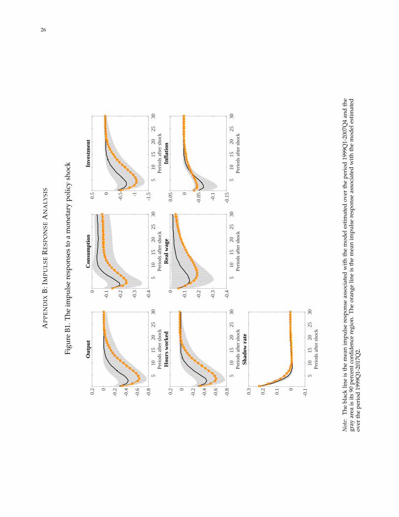
increase in nominal rigidities over the full sample. An impulse response analysis corroborates the
fact that the responses to a monetary policy shock of the macroeconomic variables estimated in the
full sample are consistent with those based on the shorter sample ending in 2007Q4 (see Figure B1 of
Appendix B). This is in line with Debortoli, Gali and Gambetti (2018) who find that the dynamic re-
sponses of a number of U.S. macro variables to different shocks did not experience any major change
during the ZLB period.
Second, all estimated values are consistent with most contributions in the medium-scale DSGE
literature. With regard to the behavior of households, our estimate of the inverse of the elasticity of
labor dis-utility, ν, is equal to 2.21 and the habit parameter h rises to 0.76, indicating that the reference
for current consumption is more than 75% of past consumption. The probability that firms are not
allowed to re-optimize their price is θp ≈ 0.89, implying an average duration of price contracts of
about two years. With respect to wages, the probability of no change is θw ≈ 0.76, implying an
average duration of wage contracts of about 12 months. All these numbers are consistent with the
results reported in the survey by Druant, Fabiani, Kezdi, Lamo, Martins and Sabbatini (2012). In
addition, the wage indexation parameter is γw ≈ 0.40, which is higher than the price indexation
parameter γp ≈ 0.32. This reflects a now standard result that euro-area data do not require too high a
degree of price or wage indexation to match the persistence in the data. Monetary policy parameters(φπ, φy
)≈ (1.97, 0.23) and φs ≈ 0.81 indicate that the systematic part of monetary policy displays
gradualism and a larger weight on inflation when focusing on the full sample than on the pre-crisis
sample. Finally, as expected, we find that the volatility of the measurement errors associated with the
three shadow rates become different only when the crisis period is taken into account.
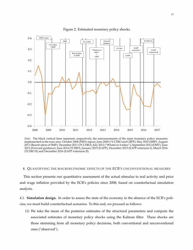
Figure 2 plots the estimated monetary policy shocks along with dates of unconventional monetary
policy announcements. We observe a crude alignment between the two: (i) during the period 2008-
2017, monetary policy shocks are essentially negative, as expected; (ii) these negative shocks coincide
with major policy announcements, such as FRFA tender, OMT, TLTRO, EAPP and TLTRO II.
5Section 2 of the Online Appendix offers additional model diagnostics (prior and posterior density plots, multivari-ate convergence diagnostics, unconditional variance decomposition) suggesting that there are no identification or stabilityissues.
13
Figure 2. Estimated monetary policy shocks
-0.4
-0.3
-0.2
-0.1
0.0
0.1
0.2
0.3
0.4
2008 2009 2010 2011 2012 2013 2014 2015 2016 2017
Reactivation
of SMP
FRFA repos
1Y-LTRO,
CBPP
SMP 3Y-LTRO
"Whatever it
takes"
+
OMT
Forward
guidance
TLTRO
EAPP
EAPP
extension I
TLTRO II
EAPP
extension II
Note: The black vertical lines represent, respectively, the announcements of the main monetary policy measuresimplemented in the euro area: October 2008 (FRFA repos), June 2009 (1Y-LTRO and CBPP), May 2010 (SMP), August2011 (Reactivation of SMP), December 2011 (3Y-LTRO), July 2012 (“Whatever it takes”), September 2012 (OMT), June2013 (Forward guidance), June 2014 (TLTRO), January 2015 (EAPP), December 2015 (EAPP extension I), March 2016(TLTRO II) and December 2016 (EAPP extension II).
4. QUANTIFYING THE MACROECONOMIC EFFECTS OF THE ECB’S UNCONVENTIONAL MEASURES
This section presents our quantitative assessment of the actual stimulus to real activity and price
and wage inflation provided by the ECB’s policies since 2008, based on counterfactual simulation
analysis.
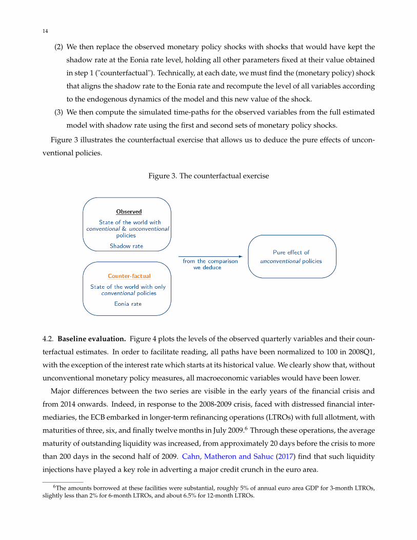
4.1. Simulation design. In order to assess the state of the economy in the absence of the ECB’s poli-
cies, we must build counterfactual scenarios. To this end, we proceed as follows:
(1) We take the mean of the posterior estimates of the structural parameters and compute the
associated estimates of monetary policy shocks using the Kalman filter. These shocks are
those stemming from all monetary policy decisions, both conventional and unconventional
ones ("observed").
14
(2) We then replace the observed monetary policy shocks with shocks that would have kept the
shadow rate at the Eonia rate level, holding all other parameters fixed at their value obtained
in step 1 ("counterfactual"). Technically, at each date, we must find the (monetary policy) shock
that aligns the shadow rate to the Eonia rate and recompute the level of all variables according
to the endogenous dynamics of the model and this new value of the shock.
(3) We then compute the simulated time-paths for the observed variables from the full estimated
model with shadow rate using the first and second sets of monetary policy shocks.
Figure 3 illustrates the counterfactual exercise that allows us to deduce the pure effects of uncon-
ventional policies.
Figure 3. The counterfactual exercise
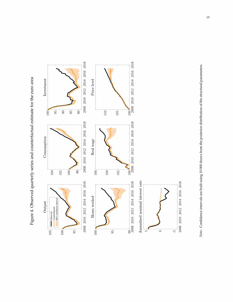
4.2. Baseline evaluation. Figure 4 plots the levels of the observed quarterly variables and their coun-
terfactual estimates. In order to facilitate reading, all paths have been normalized to 100 in 2008Q1,
with the exception of the interest rate which starts at its historical value. We clearly show that, without
unconventional monetary policy measures, all macroeconomic variables would have been lower.
Major differences between the two series are visible in the early years of the financial crisis and
from 2014 onwards. Indeed, in response to the 2008-2009 crisis, faced with distressed financial inter-
mediaries, the ECB embarked in longer-term refinancing operations (LTROs) with full allotment, with
maturities of three, six, and finally twelve months in July 2009.6 Through these operations, the average
maturity of outstanding liquidity was increased, from approximately 20 days before the crisis to more
than 200 days in the second half of 2009. Cahn, Matheron and Sahuc (2017) find that such liquidity
injections have played a key role in adverting a major credit crunch in the euro area.
6The amounts borrowed at these facilities were substantial, roughly 5% of annual euro area GDP for 3-month LTROs,slightly less than 2% for 6-month LTROs, and about 6.5% for 12-month LTROs.
15
Figu
re4.
Obs
erve
dqu
arte
rly
seri
esan
dco
unte
rfac
tual
esti
mat
efo
rth
eeu
roar
ea
2008
2010
2012
2014
2016
2018
95100
105
Outp
ut
Obs
erve
dC
ount
erfa
ctua
l68
% c
onfi
denc
e in
terv
al
2008
2010
2012
2014
2016
2018
98100
102
104
Con
sum
ption
2008
2010
2012
2014
2016
2018
80859095100
Inve
stm
ent
2008
2010
2012
2014
2016
2018
9095100
Hou
rswor
ked
2008
2010
2012
2014
2016
2018
100
102
104
106
Rea
lwag
e
2008
2010
2012
2014
2016
2018
100
105
110
Price
leve
l
2008
2010
2012
2014
2016
2018
-505Annual
ised
nom
inal
inte
rest
rate
Not
e:C
onfid
ence
inte
rval
sar
ebu
iltus
ing
1000
0dr
aws
from
the
post
erio
rdi
stri
buti
onof
the
stru
ctur
alpa
ram
eter
s.

16
Since 2014, the macroeconomic climate in the euro area has been characterized by increased risks
threatening price stability and the anchoring of inflation expectations. In this context, the ECB adopted
a threefold response (see, Marx et al., 2016). First, there was a succession of cuts in the deposit facility
rate, from 0% in early 2014 to -0.40% in March 2016. These rate-cuts complemented the forward guid-
ance policy already put in place since July 2013.7 Second, in order to increase support for lending,
a targeted longer-term refinancing operations (TLTRO) program, with attractive associated interest
rates over a period of two years, has been implemented in July 2014. The objective of TLTROs is to: (i)
encourage banks to lend more to non-financial corporations and to households and (ii) send a signal
about future short-term rates, since loans were allotted fully and at a fixed rates (with early repayment
possible without penalty). Third, public and private sector asset purchase programs have been con-
ducted. In October 2014, the Eurosystem launched a first package of quantitative easing in the form of
a dual purchase program of private sector assets aimed at promoting high-quality securitization and
reducing the risk premium inflating the lending rates to Non-Financial Corporations (NFCs). In Jan-
uary 2015, the ECB decided to expand the previous asset purchase program to include public sector
securities. The monthly purchases of public and private sector securities under this expanded asset
purchase program were carried out between March 2015 and March 2016 for a total amount of EUR 60
billion per month. In December 2015, the asset purchase program was extended until at least March
2017. In March 2016 the ECB announced a new extension of the program, comprising of an increase
in the monthly amount of purchases under the asset purchase program from EUR 60 billion to EUR
80 billion, the inclusion of investment grade bonds issued by NFCs in the scope of the asset purchase
program, and the launch of a series of four targeted longer-term refinancing operations (TLTRO II).
In December 2016 the ECB announced a recalibration of the asset purchase program, extending the
net purchases until December 2017 but at a reduced monthly pace of EUR 60 billion from April 2017.
The net purchases are to be made alongside reinvestments of the principal payments from maturing
securities purchased under the asset purchase program.8
Our results show that quarterly output would have been 4.5% lower in 2017Q2 were it not for
unconventional policies. The preponderance of this effect stems from the large decline in quarterly
investment, which would have been about 8% below its actual level. The difference in the price level
is more modest (around 2.6% in 2017Q2). The muted effect of QE on inflation, relative to GDP, is
corroborated by Andrade, Breckenfelder, De Fiore, Karadi and Tristani (2016) and Sahuc (2016). More
importantly, we note that unconventional measures have helped avoid a period of deflation from
7This forward guidance corresponds to a commitment on the future path of interest rates, so as to influence not only theshort-term rates but also longer-term rates which are largely determined by expectations of future short-term rates.
8The ECB also adjusted the parameters of the APP as of January 2017 as follows. First, the maturity range of the publicsector purchase program will be broadened by decreasing the minimum remaining maturity for eligible securities from twoyears to one year. Second, purchases of securities under the APP with a yield to maturity below the interest rate on theECB’s deposit facility will be permitted to the extent necessary.
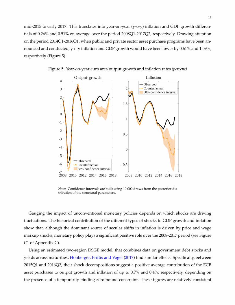
17
mid-2015 to early 2017. This translates into year-on-year (y-o-y) inflation and GDP growth differen-
tials of 0.26% and 0.51% on average over the period 2008Q1-2017Q2, respectively. Drawing attention
on the period 2014Q1-2016Q1, when public and private sector asset purchase programs have been an-
nounced and conducted, y-o-y inflation and GDP growth would have been lower by 0.61% and 1.09%,
respectively (Figure 5).
Figure 5. Year-on-year euro area output growth and inflation rates (percent)
2008 2010 2012 2014 2016 2018-7
-6
-5
-4
-3
-2
-1
0
1
2
3
4Output growth
ObservedCounterfactual68% confidence interval
2008 2010 2012 2014 2016 2018
-0.5
0
0.5
1
1.5
2
In.ation
ObservedCounterfactual68% confidence interval
Note: Confidence intervals are built using 10 000 draws from the posterior dis-tribution of the structural parameters.
Gauging the impact of unconventional monetary policies depends on which shocks are driving
fluctuations. The historical contribution of the different types of shocks to GDP growth and inflation
show that, although the dominant source of secular shifts in inflation is driven by price and wage
markup shocks, monetary policy plays a significant positive role over the 2008-2017 period (see Figure
C1 of Appendix C).
Using an estimated two-region DSGE model, that combines data on government debt stocks and
yields across maturities, Hohberger, Priftis and Vogel (2017) find similar effects. Specifically, between
2015Q1 and 2016Q2, their shock decompositions suggest a positive average contribution of the ECB
asset purchases to output growth and inflation of up to 0.7% and 0.4%, respectively, depending on
the presence of a temporarily binding zero-bound constraint. These figures are relatively consistent
18
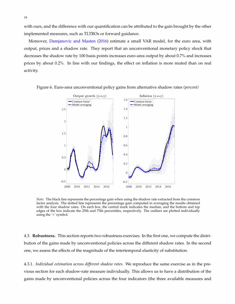
with ours, and the difference with our quantification can be attributed to the gain brought by the other
implemented measures, such as TLTROs or forward guidance.
Moreover, Damjanovic and Masten (2016) estimate a small VAR model, for the euro area, with
output, prices and a shadow rate. They report that an unconventional monetary policy shock that
decreases the shadow rate by 100 basis points increases euro-area output by about 0.7% and increases
prices by about 0.2%. In line with our findings, the effect on inflation is more muted than on real
activity.
Figure 6. Euro-area unconventional policy gains from alternative shadow rates (percent)
2008 2010 2012 2014 2016
-0.5
0
0.5
1
1.5
2
2.5
Output growth (y-o-y)
Common factorModel averaging
2008 2010 2012 2014 2016
-0.2
0
0.2
0.4
0.6
0.8
1
1.2
1.4
1.6In.ation (y-o-y)
Common factorModel averaging
Note: The black line represents the percentage gain when using the shadow rate extracted from the commonfactor analysis. The dotted line represents the percentage gain computed in averaging the results obtainedwith the four shadow rates. On each box, the central mark indicates the median, and the bottom and topedges of the box indicate the 25th and 75th percentiles, respectively. The outliers are plotted individuallyusing the ’+’ symbol.
4.3. Robustness. This section reports two robustness exercises. In the first one, we compute the distri-
bution of the gains made by unconventional policies across the different shadow rates. In the second
one, we assess the effects of the magnitude of the intertemporal elasticity of substitution.
4.3.1. Individual estimation across different shadow rates. We reproduce the same exercise as in the pre-
vious section for each shadow-rate measure individually. This allows us to have a distribution of the
gains made by unconventional policies across the four indicators (the three available measures and
19
the latent common factor). A standardized way of displaying such a distribution is to use a non-
parametric box plot that graphically depicts the gains through their quartiles. Figure 6 shows box
plots for y-o-y output growth and y-o-y inflation rates and provides two interesting results. First, the
distribution can be quite large when shadow rates fall into negative territory, with deviations up to
1% for output growth and 0.5% for inflation. Second, to account for the uncertainty surrounding the
shadow rate, an econometrician could prefer using an average of the results obtained with each of
the available indicators ("model averaging"). In this case, we see that the gains are similar to those
obtained using the "common factor" indicator.
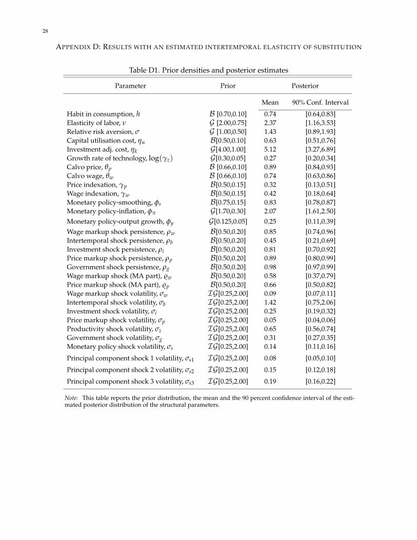
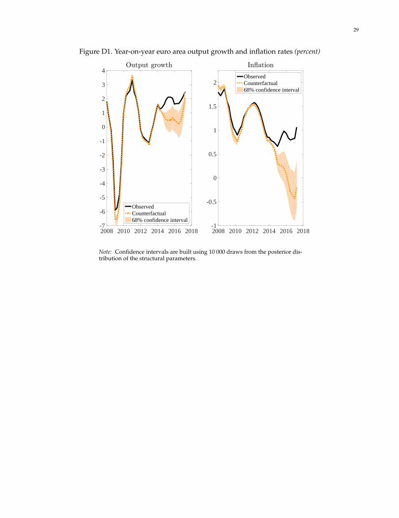
4.3.2. Estimation of the degree of relative risk aversion. Given that the magnitude of the intertemporal
elasticity of substitution changes the responsiveness of consumption relative to the interest rate, we
re-estimate our model by replacing the logarithmic specification of the utility of consumption by a
CES specification:
Et
∞
∑s=0
βsεb,t+s
((Ct+s − hCt+s−1)
1−σ − 11− σ
− Z1−σt
N1+νj,t+s
1 + ν+ V (Gt+s)
).
The key findings are the following. First, the estimate of the inverse of the intertemporal elasticity of
substitution σ is equal to 1.43, a value close to the one obtained by Smets and Wouters (2007) (see Table
D1 in Appendix D). Importantly, the calibrated value of 1 (logarithmic specification) happens to fall
within the confidence interval of the estimation of the CES specification. Second, counterfactuals are
very similar: the y-o-y inflation and GDP growth would have been on average about 0.74% and 0.96%
below their actual levels over the period 2014Q1-2017Q2, respectively (see Figure D1 in Appendix D).
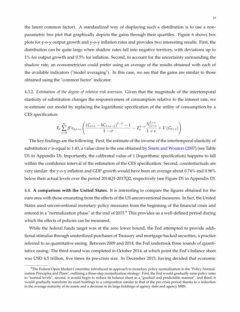
4.4. A comparison with the United States. It is interesting to compare the figures obtained for the
euro area with those emanating from the effects of the US unconventional measures. In fact, the United
States used unconventional monetary policy measures from the beginning of the financial crisis and
entered in a "normalization phase" at the end of 2015.9 This provides us a well-defined period during
which the effects of policies can be measured.
While the federal funds target was at the zero lower bound, the Fed attempted to provide addi-
tional stimulus through unsterilized purchases of Treasury and mortgage-backed securities, a practice
referred to as quantitative easing. Between 2009 and 2014, the Fed undertook three rounds of quanti-
tative easing. The third round was completed in October 2014, at which point the Fed’s balance sheet
was USD 4.5 trillion, five times its pre-crisis size. In December 2015, having decided that economic
9The Federal Open Market Committee introduced its approach to monetary policy normalization in the "Policy Normal-ization Principles and Plans", outlining a three-step normalization strategy: First, the Fed would gradually raise policy ratesto "normal levels", second, it would begin to reduce its balance sheet in a "gradual and predictable manner", and third, itwould gradually transform its asset holdings to a composition similar to that of the pre-crisis period thanks to a reductionin the average maturity of its assets and a decrease in its large holdings of agency debt and agency MBS.
20
conditions and the economic outlook warranted a rate hike, it raised its target federal funds rate for
the first time in seven years to a range of between 0.25% and 0.5%. The Fed has raised interest rates in
the presence of a large balance sheet through the use of two new tools, by raising the rate of interest
paid to banks on reserves and by engaging in reverse repurchase agreements (reverse repos) through
a new overnight facility.
We therefore reproduce an exercise identical to that carried out for the euro area but in estimating
the DSGE model on US data (over the period 1999Q1-2017Q2).10 We obtain year-on-year (y-o-y) in-
flation and GDP growth differentials of 0.6% and 0.92% on average over the period 2008Q1-2015Q4,
respectively (Figure 7).
Two points of comparison are interesting to put forward. Unlike in the euro area, the effects are
more homogeneous, probably due to the three rounds of quantitative easing over the period. Second,
while the euro area has not yet entered a normalization stage, the average macroeconomic effects (up
to 2017Q2) are of the same order than the transatlantic ones (until 2015Q4).
Figure 7. Year-on-year US output growth and inflation rates (percent)
2008 2010 2012 2014 2016-5
-4
-3
-2
-1
0
1
2
3
4Output growth
ObservedCounterfactual68% confidence interval
2008 2010 2012 2014 2016-0.5
0
0.5
1
1.5
2
2.5In.ation
ObservedCounterfactual68% confidence interval
Note: Confidence intervals are built using 10 000 draws from the posterior dis-tribution of the structural parameters.
10US data are taken from the FRED database: GDP growth (GDPC96), consumption growth (PCEC), investment growth(FPI), wage growth (PRS85006103), weekly hours (PRS85006023), GDP deflator (GDPDEF), core PCE (JCXFE), civilianemployment (CE16OV), civilian non-institutional population (LNU00000000Q), Federal funds rate (FEDFUNDS). The USshadow rate is the one by Wu and Xia (2016). A comparison of the fed funds rate and the shadow rate is provided in FigureOA3 of the Online Appendix.
21
5. CONCLUDING REMARKS
In this paper, we estimate a medium-scale DSGE model in which the policy rate is replaced by a
shadow rate, and perform counterfactual analyses. This allows us to quantify the macroeconomic
effects of the European Central Bank’s unconventional monetary policies. Overall, our results suggest
that, without unconventional measures, the euro area would have suffered (i) a substantial loss of
output since the Great Recession and (ii) a period of deflation from mid-2015 to early 2017. This
translates into year-on-year inflation and GDP growth differentials of 0.61% and 1.09%, respectively,
over the period 2014Q1-2017Q2.
Our analysis also highlights that we can still use standard DSGE models in low interest rate envi-
ronments when using an unconstrained proxy of the monetary policy stance such as the shadow rate.
Indeed, the introduction of the shadow rate allows us to bypass problems associated with the ELB,
especially when the latter varies over time as in the euro area. It makes the approach appealing from
a policy point of view because evaluations can be easily made using traditional tools.
However, there are many extensions to this current work, both from a modeling and an econometric
perspective. In particular, endogenously deriving the shadow rate within the structural model, by
attempting to directly introduce a term structure into the model (along the lines of Ang and Piazzesi,
2003; Hordahl et al., 2006) would be a promising step. The complexity is that the shadow rate block
remains nonlinear and therefore solving and estimating the model as a whole is not trivial.

22
REFERENCES
An S, Schorfheide F. 2007. Bayesian Analysis of DSGE Models. Econometric Reviews 26: 113–172.Andrade P, Breckenfelder J, De Fiore F, Karadi P, Tristani O. 2016. The ECB’s asset purchase pro-
gramme: an early assessment. Working Paper Series 1956, European Central Bank.Ang A, Piazzesi M. 2003. A no-arbitrage vector autoregression of term structure dynamics with
macroeconomic and latent variables. Journal of Monetary Economics 50: 745–787.Baumeister C, Benati L. 2013. Unconventional Monetary Policy and the Great Recession: Estimating
the Macroeconomic Effects of a Spread Compression at the Zero Lower Bound. International Journalof Central Banking 9: 165–212.
Benati L. 2010. Are policy counterfactuals based on structural VAR’s reliable? Working Paper Series1188, European Central Bank.
Bhattarai S, Neely CJ. 2016. A Survey of the Empirical Literature on U.S. Unconventional MonetaryPolicy. Working Papers 2016-21, Federal Reserve Bank of St. Louis.
Cahn C, Matheron J, Sahuc J. 2017. Assessing the Macroeconomic Effects of LTROs during the GreatRecession. Journal of Money, Credit and Banking 49: 1443–1482.
Cai M, Del Negro M, Giannoni M, Gupta A, Li P, Moszkowski E. 2018. DSGE forecasts of the lostrecovery. Staff Reports 844, Federal Reserve Bank of New York.
Chen H, Cúrdia V, Ferrero A. 2012. The Macroeconomic Effects of Large-scale Asset Purchase Pro-grammes. Economic Journal 122: F289–F315.
Christensen JH, Rudebusch GD. 2016. Modeling yields at the zero lower bound: are shadow rates thesolution? In Advances in Econometrics, volume 35. Emerald Group Publishing Limited, 75–125.
Christensen JHE, Rudebusch GD. 2015. Estimating Shadow-Rate Term Structure Models with Near-Zero Yields. Journal of Financial Econometrics 13: 226–259.
Christiano L, Eichenbaum M, Trabandt M. 2017. On DSGE Models. Mimeo, Northwestern University.Claus E, Claus I, Krippner L. 2014. Asset markets and monetary policy shocks at the zero lower bound.
Reserve Bank of New Zealand Discussion Paper Series DP2014/03, Reserve Bank of New Zealand.Cova P, Pagano P, Pisani M. 2015. Domestic and international macroeconomic effects of the Eurosys-
tem expanded asset purchase programme. Temi di discussione (Economic working papers) 1036,Bank of Italy, Economic Research and International Relations Area.
Damjanovic M, Masten I. 2016. Shadow short rate and monetary policy in the Euro area. Empirica 43:279–298.
Debortoli D, Gali J, Gambetti L. 2018. On the Empirical (Ir)Relevance of the Zero Lower Bound Con-straint. Working Papers 1013, Barcelona Graduate School of Economics.
Del Negro M, Eggertsson G, Ferrero A, Kiyotaki N. 2017. The Great Escape? A Quantitative Evaluationof the Fed’s Liquidity Facilities. American Economic Review 107: 824–857.
Del Negro M, Giannoni M, Patterson C. 2015. The Forward Guidance Puzzle. 2015 Meeting Papers1529, Society for Economic Dynamics.
Doh T, Choi J. 2016. Measuring the Stance of Monetary Policy on and off the Zero Lower Bound.Technical Report Q III, Federal Reserve Bank of Kansas City.
Druant M, Fabiani S, Kezdi G, Lamo A, Martins F, Sabbatini R. 2012. Firms’ price and wage adjustmentin Europe: Survey evidence on nominal stickiness. Labour Economics 19: 772–782.
23
Engen EM, Laubach T, Reifschneider DL. 2015. The Macroeconomic Effects of the Federal Reserve’sUnconventional Monetary Policies. Finance and Economics Discussion Series 2015-5, Board of Gov-ernors of the Federal Reserve System (U.S.).
Everaert L, Schule W. 2008. Why It Pays to Synchronize Structural Reforms in the Euro Area AcrossMarkets and Countries. IMF Staff Papers 55: 356–366.
Francis N, Jackson LE, Owyang MT. 2014. How has empirical monetary policy analysis changed afterthe financial crisis? Working Papers 2014-19, Federal Reserve Bank of St. Louis.
Gertler M, Karadi P. 2013. QE 1 vs. 2 vs. 3. . . : A Framework for Analyzing Large-Scale Asset Purchasesas a Monetary Policy Tool. International Journal of Central Banking 9: 5–53.
Hakkio CS, Kahn GA. 2014. Evaluating monetary policy at the zero lower bound. Technical Report QII, Federal Reserve Bank of Kansas City.
Hohberger S, Priftis R, Vogel L. 2017. The macroeconomic effects of quantitative easing in the Euroarea : evidence from an estimated DSGE model. Economics Working Papers ECO2017/04, EuropeanUniversity Institute.
Hordahl P, Tristani O, Vestin D. 2006. A joint econometric model of macroeconomic and term-structuredynamics. Journal of Econometrics 131: 405–444.
Justiniano A, Primiceri GE, Tambalotti A. 2010. Investment shocks and business cycles. Journal ofMonetary Economics 57: 132–145.
Kim DH, Singleton KJ. 2012. Term structure models and the zero bound: An empirical investigationof Japanese yields. Journal of Econometrics 170: 32–49.
Kortela T. 2016. A shadow rate model with time-varying lower bound of interest rates. ResearchDiscussion Papers 19/2016, Bank of Finland.
Krippner L. 2012. Modifying gaussian term structure models when interest rates are near the zerolower bound. Reserve Bank of New Zealand Discussion Paper Series DP2012/02, Reserve Bank ofNew Zealand.
Krippner L. 2013. Measuring the stance of monetary policy in zero lower bound environments. Eco-nomics Letters 118: 135–138.
Kulish M, Morley J, Robinson T. 2017. Estimating DSGE models with Zero Interest Rate Policy. Journalof Monetary Economics 88: 35–49.
Lemke W, Vladu AL. 2016. Below the zero lower bound: A shadow-rate term structure model for theeuro area. Discussion Papers 32/2016, Deutsche Bundesbank, Research Centre.
Lucas RJ. 1976. Econometric policy evaluation: A critique. Carnegie-Rochester Conference Series on PublicPolicy 1: 19–46.
Marx M, Nguyen B, Sahuc JG. 2016. Monetary policy measures in the euro area and their effects since2014. Rue de la Banque (Banque de France) 32.
McAdam P, Willman A. 2013. Medium Run Redux. Macroeconomic Dynamics 17: 695–727.McKay A, Nakamura E, Steinsson J. 2016. The Power of Forward Guidance Revisited. American
Economic Review 106: 3133–3158.Sahuc JG. 2016. The ECB’s asset purchase programme: a model-based evaluation. Economics Letters
145: 136–140.Sahuc JG, Smets F. 2008. Differences in Interest Rate Policy at the ECB and the Fed: An Investigation
with a Medium-Scale DSGE Model. Journal of Money, Credit and Banking 40: 505–521.

24
Smets F, Wouters R. 2007. Shocks and Frictions in US Business Cycles: A Bayesian DSGE Approach.American Economic Review 97: 586–606.
Van Zandweghe W. 2015. Monetary Policy Shocks and Aggregate Supply. Economic Review : 31–56.Weale M, Wieladek T. 2016. What are the macroeconomic effects of asset purchases? Journal of Monetary
Economics 79: 81–93.Wu JC, Xia FD. 2016. Measuring the Macroeconomic Impact of Monetary Policy at the Zero Lower
Bound. Journal of Money, Credit and Banking 48: 253–291.Wu JC, Xia FD. 2017. Time-Varying Lower Bound of Interests in Europe. Chicago Booth Research
Paper 17-06, Chicago Booth.Wu JC, Zhang J. 2017. A Shadow Rate New Keynesian Model. Chicago Booth Research Paper 16-18,
Chicago Booth.
25
APPENDIX A: SHADOW RATE AND KEY FINANCIAL INDICATORS
Figure A1. Private and public interest rates, financial condition index, and the shadow rate
2008 2009 2010 2011 2012 2013 2014 2015 2016 2017-4
-3
-2
-1
0
1
2
3
4
5
6
98.5
99
99.5
100
100.5
101
101.5
102
102.5
Shadow rate (lhs)Deposits with agreed maturity (lhs)Loans to NFCs, over 5 years (lhs)Government Bond 3M (lhs)Goldman Sachs FCI (rhs)
Note: The orange line is the representative shadow rate (obtained as a commoncomponent of three alternative shadow rates) and the green lines represent: (i)the rate on deposits with agreed maturity for households (mainly time depositswith a given maturity that may be subject to the payment of a penalty in theevent of early withdrawal); (ii) the rate on loans to Non-Financial Corpora-tions (NFC) with maturity over 5 years; (iii) the nominal 3-month governmentbond yield, all issuers whose rating is between AAA and AA; (iv) the euro-area Goldman Sachs Financial Condition Index (FCI). Deposits and loans arenew business. The source of private and public rates is the ECB-Statistical DataWarehouse and the source of the Goldman-Sachs FCI is Bloomberg.
26
AP
PE
ND
IXB
:IM
PU
LSE
RE
SPO
NSE
AN
ALY
SIS
Figu
reB1
.The
impu
lse
resp
onse
sto
am
onet
ary
polic
ysh
ock
510
1520
2530
Peri
ods
afte
r sh
ock
-0.8
-0.6
-0.4
-0.20
0.2
Out
put
510
1520
2530
Peri
ods
afte
r sh
ock
-0.4
-0.3
-0.2
-0.10
Con
sum
ptio
n
510
1520
2530
Peri
ods
afte
r sh
ock
-1.5-1
-0.50
0.5
Inve
stm
ent
510
1520
2530
Peri
ods
afte
r sh
ock
-0.8
-0.6
-0.4
-0.20
0.2
Hou
rs w
orke
d
510
1520
2530
Peri
ods
afte
r sh
ock
-0.4
-0.3
-0.2
-0.10
Rea
l wag
e
510
1520
2530
Peri
ods
afte
r sh
ock
-0.1
5
-0.1
-0.0
50
0.05
Infl
atio
n
510
1520
2530
Peri
ods
afte
r sh
ock
-0.10
0.1
0.2
0.3
Shad
ow r
ate
Not
e:Th
ebl
ack
line
isth
em
ean
impu
lse
resp
onse
asso
ciat
edw
ith
the
mod
eles
tim
ated
over
the
peri
od19
99Q
1-20
07Q
4an
dth
egr
ayar
eais
its
90pe
rcen
tcon
fiden
cere
gion
.Th
eor
ange
line
isth
em
ean
impu
lse
resp
onse
asso
ciat
edw
ith
the
mod
eles
tim
ated
over
the
peri
od19
99Q
1-20
17Q
2.

27
APPENDIX C: HISTORICAL DECOMPOSITION OF GDP GROWTH AND INFLATION
Figure C1. Historical decomposition of GDP growth (top) and inflation (bottom)
-5
-4
-3
-2
-1
0
1
2
Demand Markup Productivity Monetary Policy GDP Growth
-0,5
-0,4
-0,3
-0,2
-0,1
0
0,1
0,2
0,3
0,4
Demand Markup Productivity Monetary Policy Inflation
Note: The demand shocks include the preference, investment and government spend-ing shocks; the markup shocks include the price and wage markup shocks. Quarterlymean inflation is estimated at 0.35 percent.
28
APPENDIX D: RESULTS WITH AN ESTIMATED INTERTEMPORAL ELASTICITY OF SUBSTITUTION
Table D1. Prior densities and posterior estimates
Parameter Prior Posterior
Mean 90% Conf. Interval
Habit in consumption, h B [0.70,0.10] 0.74 [0.64,0.83]Elasticity of labor, ν G [2.00,0.75] 2.37 [1.16,3.53]Relative risk aversion, σ G [1.00,0.50] 1.43 [0.89,1.93]Capital utilisation cost, ηu B[0.50,0.10] 0.63 [0.51,0.76]Investment adj. cost, ηk G[4.00,1.00] 5.12 [3.27,6.89]Growth rate of technology, log(γz) G[0.30,0.05] 0.27 [0.20,0.34]Calvo price, θp B [0.66,0.10] 0.89 [0.84,0.93]Calvo wage, θw B [0.66,0.10] 0.74 [0.63,0.86]Price indexation, γp B[0.50,0.15] 0.32 [0.13,0.51]Wage indexation, γw B[0.50,0.15] 0.42 [0.18,0.64]Monetary policy-smoothing, φs B[0.75,0.15] 0.83 [0.78,0.87]Monetary policy-inflation, φπ G[1.70,0.30] 2.07 [1.61,2.50]Monetary policy-output growth, φy G[0.125,0.05] 0.25 [0.11,0.39]Wage markup shock persistence, ρw B[0.50,0.20] 0.85 [0.74,0.96]Intertemporal shock persistence, ρb B[0.50,0.20] 0.45 [0.21,0.69]Investment shock persistence, ρi B[0.50,0.20] 0.81 [0.70,0.92]Price markup shock persistence, ρp B[0.50,0.20] 0.89 [0.80,0.99]Government shock persistence, ρg B[0.50,0.20] 0.98 [0.97,0.99]Wage markup shock (MA part), $w B[0.50,0.20] 0.58 [0.37,0.79]Price markup shock (MA part), $p B[0.50,0.20] 0.66 [0.50,0.82]Wage markup shock volatility, σw IG[0.25,2.00] 0.09 [0.07,0.11]Intertemporal shock volatility, σb IG[0.25,2.00] 1.42 [0.75,2.06]Investment shock volatility, σi IG[0.25,2.00] 0.25 [0.19,0.32]Price markup shock volatility, σp IG[0.25,2.00] 0.05 [0.04,0.06]Productivity shock volatility, σz IG[0.25,2.00] 0.65 [0.56,0.74]Government shock volatility, σg IG[0.25,2.00] 0.31 [0.27,0.35]Monetary policy shock volatility, σs IG[0.25,2.00] 0.14 [0.11,0.16]
Principal component shock 1 volatility, σs1 IG[0.25,2.00] 0.08 [0.05,0.10]
Principal component shock 2 volatility, σs2 IG[0.25,2.00] 0.15 [0.12,0.18]
Principal component shock 3 volatility, σs3 IG[0.25,2.00] 0.19 [0.16,0.22]
Note: This table reports the prior distribution, the mean and the 90 percent confidence interval of the esti-mated posterior distribution of the structural parameters.
29
Figure D1. Year-on-year euro area output growth and inflation rates (percent)
2008 2010 2012 2014 2016 2018-7
-6
-5
-4
-3
-2
-1
0
1
2
3
4Output growth
ObservedCounterfactual68% confidence interval
2008 2010 2012 2014 2016 2018-1
-0.5
0
0.5
1
1.5
2
In.ation
ObservedCounterfactual68% confidence interval
Note: Confidence intervals are built using 10 000 draws from the posterior dis-tribution of the structural parameters.


