Download - EXPERIMENTAL INVESTIGATION OF INLET AIR TEMPERATURE ROTARY …

EXPERIMENTAL INVESTIGATION OF INLET AIR TEMPERATURE

ON INPUT POWER IN AN OIL-FLOODED

ROTARY SCREW AIR COMPRESSOR

by

MING HAN CHUA

KEITH A. WOODBURY, COMMITTEE CHAIR

GARY P. MOYNIHAN

JOSHUA A. BITTLE

A THESIS

Submitted in partial fulfillment of the requirements

for the degree of Master of Science

in the Department of Mechanical Engineering

in the Graduate School of

The University of Alabama

TUSCALOOSA, ALABAMA

2015

Copyright Ming Han Chua 2015

ALL RIGHTS RESERVED

ii

ABSTRACT

For operation of industrial air compressors, conventional wisdom dictates that breathing

outside air, which has lower temperature, will reduce the air compressor power consumption. In

addition, many energy professionals and reliable sources (Parekh, 2000; Kaya et al., 2002; U.S

Department of Energy, 2004; Hick, 2006) advocate the use of cooler air to reduce compressor

power consumption. However, experimental results are not available to support the conventional

wisdom.

The purpose of this thesis is to experimentally investigate the effect of inlet air

temperature on an oil-flooded rotary screw compressor located in the University of Alabama.

This experiment is set up in a controlled environment. More specifically, a data acquisition

system with digitally controlled fluids is developed to control the air demand imposed on the

compressor. A range of inlet air temperatures are investigated based on local weather conditions.

The injected oil temperature can be modified slightly by restricting the air flow through the air

cooler.

A design of experiments technique is utilized to evaluate the influence of inlet air

temperature, inlet oil temperature, and air flow rate on the compressor power. The results show

that inlet air temperature has little or no contribution to the compressor power. Moreover, the

collected data shows that power consumption does not vary with inlet oil temperature. The

results also show that as the inlet air temperature increases, the isentropic efficiency increases.

iii

LIST OF ABBREVIATIONS AND SYMBOLS

W power consumption by the air compressor

�� intake air mass flow rate

k isentropic value

R universal gas constant

T1 inlet air temperature

ηisen isentropic efficiency

P2 pressure after the compression

P1 pressure of the intake air

𝑉1 intake air volume flow rate

Z1 compressibility correction for gas in the inlet

Z2 compressibility correction for gas at the discharge

Pr, air reduced pressure

Tr air reduced temperature

P gas pressure at present state

Pc respective gas critical pressure

T gas temperature at present state

Tc respective gas critical temperature

Iindoor indoor required intake volume

Ioutoor outdoor required intake volume

iv

𝑃𝑠 power saving in percentage

𝜌70˚F density of air at 70 ˚F,

𝜌90˚F density of air at 90 ˚F

𝜌50˚F density of air at 50 ˚F

WR energy saving fraction

Tindoor indoor temperature

Toutdoor outdoor temperature

𝑥𝑛𝑜𝑟𝑚𝑎𝑙𝑖𝑧𝑒𝑑 design of experiment normalized value

xmeas measured value

xhigh the highest measured value

xlow the lowest measured value

𝑌 linear model dependent variable

𝛼0, 𝛼1,…, 𝛼7 independent variable linear model coefficients

w specific work input

𝑛 compression process constant value

ACFM actual cubic feet per minute

SCFM standard cubic feet per minute

Ps standard pressure

Pa atmospheric pressure

ppm partial pressure of moisture at atmospheric temperature

RH relative humidity

Ta atmospheric temperature

Ts standard temperature

v

𝑒𝑠 saturated vapor pressure

Te actual temperature to calculate saturated vapor pressure

Vair air flow rate

Tair,in inlet air temperature

Toil,in injected oil temperature

Wmeas measured compressor’s power

��𝑚𝑎𝑥 maximum volumetric air flow rate in the air hose

𝐴 cross section area of the air hose

Ma Mach number

gc specific gravity

k1 conversion factor

𝐵𝐷 blowdown flow rate

𝑡𝑙𝑜𝑎𝑑𝑒𝑑 compressor loaded time

𝑡𝑢𝑛𝑙𝑜𝑎𝑑𝑒𝑑 compressor unloaded time

𝑡𝑠ℎ𝑢𝑡𝑑𝑜𝑤𝑛 compressor shutdown time

ηmotor motor efficiency

ηtrans transmission efficiency

ρstd air density at the standard condition

𝑉𝑝𝑟𝑜𝑑 measured volumetric flow rate and estimated blowdown rate

wisen,ave average isentropic work

LF load fraction

Wisen,UL isentropic work during unloaded

vi

ACKNOWLEDGEMENTS

I would like to express my deepest appreciation to Dr. Keith Woodbury, the chairman of

my thesis committee and my principle advisor. His intelligence, guidance, inputs, and

encouragement throughout my academic career have been invaluable. Also, I would like to thank

him for the opportunity to work in the Alabama Industrial Assessment Center. Working in this

center allows me the opportunity to apply engineering concept to solve the real–world problems.

Also, I have learned a lot of analysis skills, and some are applicable in this thesis. Furthermore, I

have the opportunity to pass on the knowledge and valuable skills to my juniors. Last but not

least, I would like to thank my parents and family members for their continuously support in my

academic career.

vii

CONTENTS

ABSTRACT .................................................................................................................................... ii

LIST OF ABBREVIATIONS AND SYMBOLS .......................................................................... iii

ACKNOWLEDGEMENTS ........................................................................................................... vi

LIST OF TABLES ....................................................................................................................... xiv

LIST OF FIGURES ..................................................................................................................... xvi

CHAPTER 1: INTRODUCTION ................................................................................................... 1

1.1 Background ..................................................................................................................... 1

1.2 Motivation ....................................................................................................................... 2

1.3 Literature Review............................................................................................................ 6

1.4 Design of Experiment ................................................................................................... 10

CHAPTER 2: Air Compressor Characteristic .............................................................................. 13

2.1 Types of Air Compressor .............................................................................................. 13

2.2 Compression Processes ................................................................................................. 14

2.3 Control Strategies.......................................................................................................... 17

2.4 Volumetric Flow Rate under Different Conditions ...................................................... 18

CHAPTER 3: Experiment............................................................................................................. 20

3.2 Objective ....................................................................................................................... 20

3.3 Experiment Setup .......................................................................................................... 20

viii

3.4 Procedures ..................................................................................................................... 29

3.5 Result and Discussion ................................................................................................... 33

3.5.1 Design of Experiment ........................................................................................... 33

3F2L–CP Model................................................................................................................ 33

2F2L–CP Model................................................................................................................ 37

2F2L–IOT Model .............................................................................................................. 39

3.5.2 Thermodynamic Analysis ..................................................................................... 40

CHAPTER 4: CONCLUSIONS ................................................................................................... 53

4.1 Summary ....................................................................................................................... 53

4.2 Future Work .................................................................................................................. 54

REFERENCES ............................................................................................................................. 55

xiv

LIST OF TABLES

Table 1. 2k design “Standard Order” combination (NIST/SEMATECH, 2013). ......................... 11

Table 2. Full model matrix of a 23 design, (NIST/SEMATECH, 2013). ..................................... 12

Table 3. Summary of each valve’s model number, Cv value, and the corresponding airflow. .... 27

Table 4. Corresponding air flow rate with combination valves. ................................................... 29

Table 5. 3F2L–CP model. ............................................................................................................. 30

Table 6. 2F2L–CP and 2F2L–IOT model ..................................................................................... 30

Table 7. Group of data on each combination experiment. ............................................................ 34

Table 8. Data for 3F2L–CP model. ............................................................................................... 34

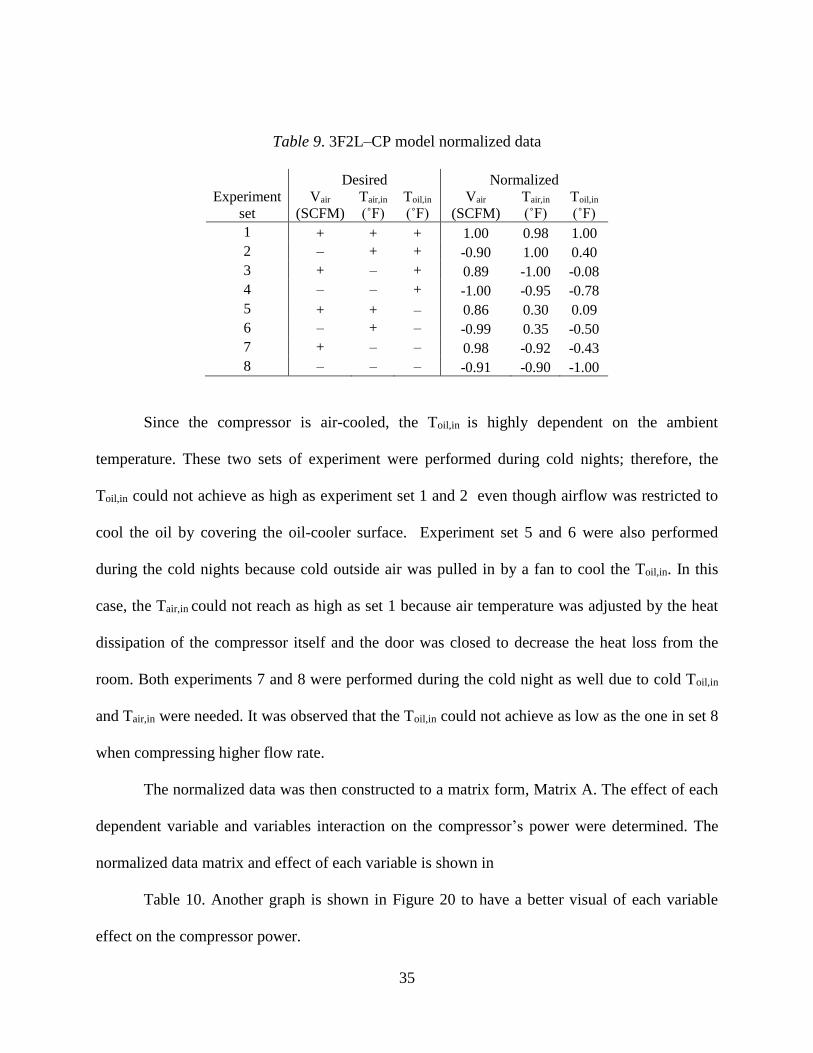
Table 9. 3F2L–CP model normalized data ................................................................................... 35

Table 10. 3F2L–CP model matrix A and effects .......................................................................... 36

Table 11. 3F2L–CP Orthogonal property ..................................................................................... 37

Table 12. 2F2L–CP model normalized data ................................................................................. 37

Table 13. 3F2L–CP model matrix B and effects .......................................................................... 38

Table 14. 2F2L–CP Orthogonal property ..................................................................................... 38

Table 15. 2F2L–IOT model matrix C and effects......................................................................... 39

Table 16. Average, range, standard deviation, and flowmeter accuracy of a

nominal 23 SCFM. ...................................................................................................... 41


nominal 48 SCFM ....................................................................................................... 42


nominal 63 SCFM. ....................................................................................................... 42

xv


nominal 75 SCFM. ....................................................................................................... 43

xvi

LIST OF FIGURES

Figure 1. Power output & efficiency versus varying inlet air temperature

(Kakaras et al., 2004). .................................................................................................... 9

Figure 2. Graphical representation of a 2k design (NIST/SEMATECH, 2013). ........................... 11

Figure 3. Different compression processes in P-v diagram (Cengel & Boles, 2011). .................. 15

Figure 4. Two-stage compression in P-v diagram (Cengel & Boles, 2011). ................................ 16

Figure 5. Two-stage compression in T-s diagram (Cengel & Boles, 2011). ................................ 16

Figure 6. Load/Unload control scheme with different air receiver capacities on

lubricant-injected rotary compressor (Office of Energy Efficiency

& Renewable Energy & Compressed Air Challenge, 2003). ....................................... 17

Figure 7. Inlet-modulating with and without unloading control scheme on

lubricant-injected rotary compressor (Office of Energy Efficiency &

Renewable Energy & Compressed Air Challenge, 2003). ........................................... 18

Figure 8. First configuration experiment set up. ........................................................................... 22

Figure 9. Insulated flexible duct connected with the air filter. ..................................................... 22

Figure 10. Fan connected with the duct to supply air. .................................................................. 23

Figure 11. Fans to increase the oil cooling rate. ........................................................................... 23

Figure 12. Flowmeter with data logger. ........................................................................................ 24

Figure 13. Flowmeter. ................................................................................................................... 24

Figure 14. Power transducer and data logger installation in the power cabinet. .......................... 25

Figure 15. Air demand simulating system. ................................................................................... 26

Figure 16. Valves and tank setup. ................................................................................................. 26

xvii

Figure 17. Overall experiment setup schematic. ........................................................................... 27

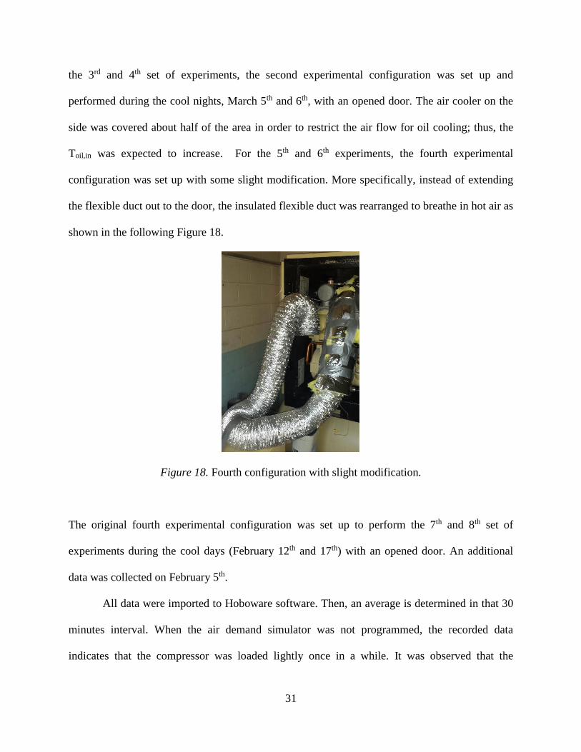
Figure 18. Fourth configuration with slight modification. ........................................................... 31

Figure 19. 30 minutes of compressor’s power draw characteristic when no air demand. ............ 32

Figure 20. 3F2L–CP model effect on compressor power. ............................................................ 36

Figure 21. 3F2L–CP model effect on compressor power. ............................................................ 38

Figure 22. 2F2L–IOT model effect on inlet oil temperature. ....................................................... 39

Figure 23. Sample of a recorded data from a day. ........................................................................ 40

Figure 24. Average measured power versus air flow rate. ........................................................... 41

Figure 25. Power versus inlet air temperature at different nominal set flow rate. ........................ 44

Figure 26. Power versus inlet oil temperature at different nominal set flow rate. ........................ 44

Figure 27. Measured specific work versus air flow at different range of inlet temperature. ........ 46

Figure 28. Measured specific work versus inlet air temperature. ................................................. 46

Figure 29. Specific work versus inlet air temperature at nominal 23 SCFM. .............................. 47




Figure 33. Isentropic efficiency versus inlet air temperature. ...................................................... 50

Figure 34. Average isentropic work versus inlet air temperature. ................................................ 51

Figure 35. Average isentropic work efficiency versus inlet air temperature. ............................... 52

1

CHAPTER 1: INTRODUCTION

Chapter 1 provides background information regarding the necessity of compressed air in

today’s world. Also, the motivation for re-evaluating the “Effect of Intake on Compressor

Performance” tip sheet is presented followed by the literature review which reveals the lack of

evidence for this “tip”. Finally, the benefit of performing design of experiment (DOE) in this

thesis is discussed.

1.1 Background

Compressed air has been vital to the manufacturing industry. Almost all manufacturing

facilities, such as food, lumber mill, pulp and paper, automaker, and foundry, have a compressed

air system for process use. It is often considered to be the “fourth utility”, behind the electricity,

water and gas. In other words, compressed air is just another type of energy source: It converts

electrical energy to compressed air energy. According to U.S Department of Energy’s Heat

Recovery Fact Sheet #10 (2003), a range from 80% to 93% of the compressor’s power input is

converted into heat. Therefore, it is expensive to produce compressed air since the input energy

is only converted to a small useful energy. Compression energy can account approximately 20%

of industrial total electric power demand (Martinez, Guillen, Prada, & Conteras, 2012). In the

Compressed Air Tip Sheet #1, a typical industrial facility’s compressed air energy usage cost

accounts about 10% of the total electric bill while some facilities account more than 30% (U.S

Department of Energy, 2004). Moreover, for a typical compressed air system, the electrical

usage cost represents a large portion (76%) of the total lifetime cost compared to the equipment

2

(12%) and maintenance (12%) cost (U.S Department of Energy, 2004). Although it is more

costly to make compressed air, it is still widely used in many industries. In this case, a lot of

research has been done to improve the overall compressed air system efficiency.

There are a lot of articles and tip sheets about improving compressed air system

published in the Department of Energy of U.S website. A few examples are shown in the

following:

(1) Alternative Strategies for Low Pressure End Uses

(2) Compressed Air Storage Strategies

(3) Minimize Compressed Air Leaks

(4) Effect of Intake on Compressor Performance

There are many consultants, engineers and others concerned about compressed air system who

will refer to these published tip sheets. In fact, energy retrofit projects on air compressors often

refer to these tip sheets; therefore, it is extremely important to provide accurate information.

1.2 Motivation

Utilizing outside air to feed the air compressor is conventional wisdom in the

manufacturing industry since it is believed less energy is consumed compressing air. The main

reason is that as the air temperature decreases, the air density increases, which results in more

molecules captured during the compression. More specifically, during compression, the air

volume is forced to shrink down, which encapsulates the same amount of molecules in a smaller

volume, to increase the pressure inside. The number of molecules in the smaller volume depends

on the initial air density which is also correlated to the air temperature. In other words, as the

cooler air is fed into the compressor, the instantaneous power consumed is less.

3

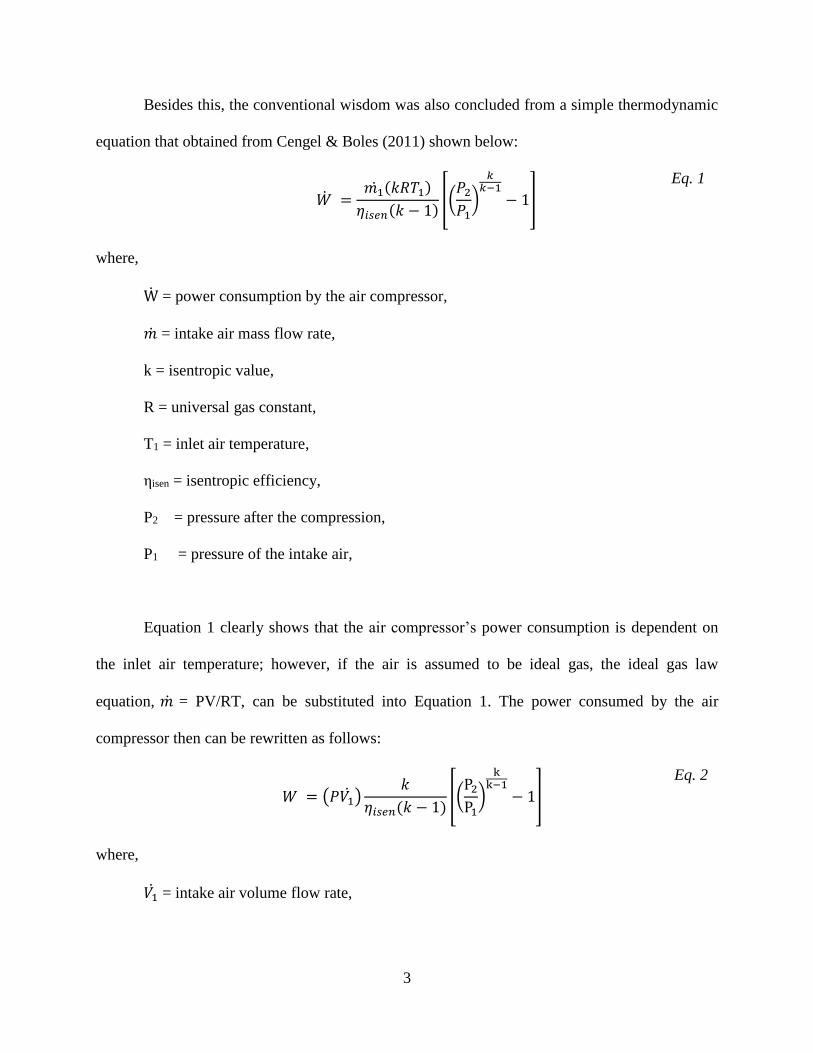
Besides this, the conventional wisdom was also concluded from a simple thermodynamic

equation that obtained from Cengel & Boles (2011) shown below:

�� =𝑚1 (𝑘𝑅𝑇1)

𝜂𝑖𝑠𝑒𝑛(𝑘 − 1)[(

𝑃2

𝑃1)

𝑘𝑘−1

− 1]

Eq. 1

where,

W = power consumption by the air compressor,

�� = intake air mass flow rate,

k = isentropic value,

R = universal gas constant,

T1 = inlet air temperature,

ηisen = isentropic efficiency,

P2 = pressure after the compression,

P1 = pressure of the intake air,

Equation 1 clearly shows that the air compressor’s power consumption is dependent on

the inlet air temperature; however, if the air is assumed to be ideal gas, the ideal gas law

equation, �� = PV/RT, can be substituted into Equation 1. The power consumed by the air

compressor then can be rewritten as follows:

𝑊 = (𝑃𝑉1)𝑘

𝜂𝑖𝑠𝑒𝑛(𝑘 − 1)[(

P2

P1)

kk−1

− 1]

Eq. 2

where,

𝑉1 = intake air volume flow rate,

4

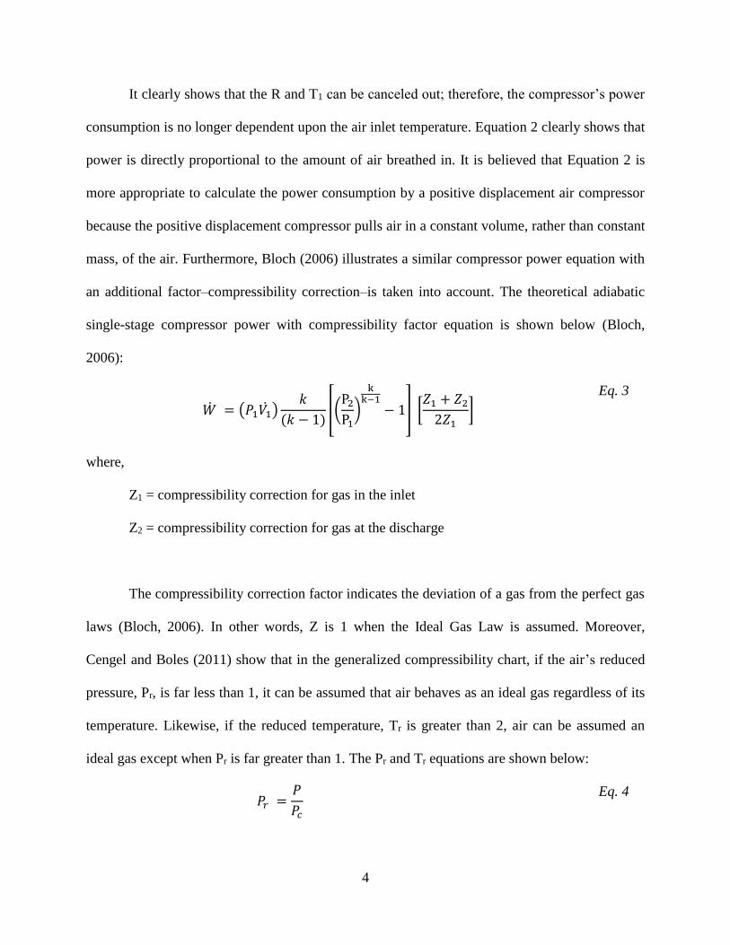
It clearly shows that the R and T1 can be canceled out; therefore, the compressor’s power

consumption is no longer dependent upon the air inlet temperature. Equation 2 clearly shows that

power is directly proportional to the amount of air breathed in. It is believed that Equation 2 is

more appropriate to calculate the power consumption by a positive displacement air compressor

because the positive displacement compressor pulls air in a constant volume, rather than constant

mass, of the air. Furthermore, Bloch (2006) illustrates a similar compressor power equation with

an additional factor–compressibility correction–is taken into account. The theoretical adiabatic

single-stage compressor power with compressibility factor equation is shown below (Bloch,

2006):

�� = (𝑃1𝑉1)𝑘

(𝑘 − 1)[(

P2

P1)

kk−1

− 1] [𝑍1 + 𝑍2

2𝑍1]

Eq. 3

where,

Z1 = compressibility correction for gas in the inlet

Z2 = compressibility correction for gas at the discharge

The compressibility correction factor indicates the deviation of a gas from the perfect gas

laws (Bloch, 2006). In other words, Z is 1 when the Ideal Gas Law is assumed. Moreover,

Cengel and Boles (2011) show that in the generalized compressibility chart, if the air’s reduced

pressure, Pr, is far less than 1, it can be assumed that air behaves as an ideal gas regardless of its

temperature. Likewise, if the reduced temperature, Tr is greater than 2, air can be assumed an

ideal gas except when Pr is far greater than 1. The Pr and Tr equations are shown below:

𝑃𝑟 =𝑃

𝑃𝑐

Eq. 4

5

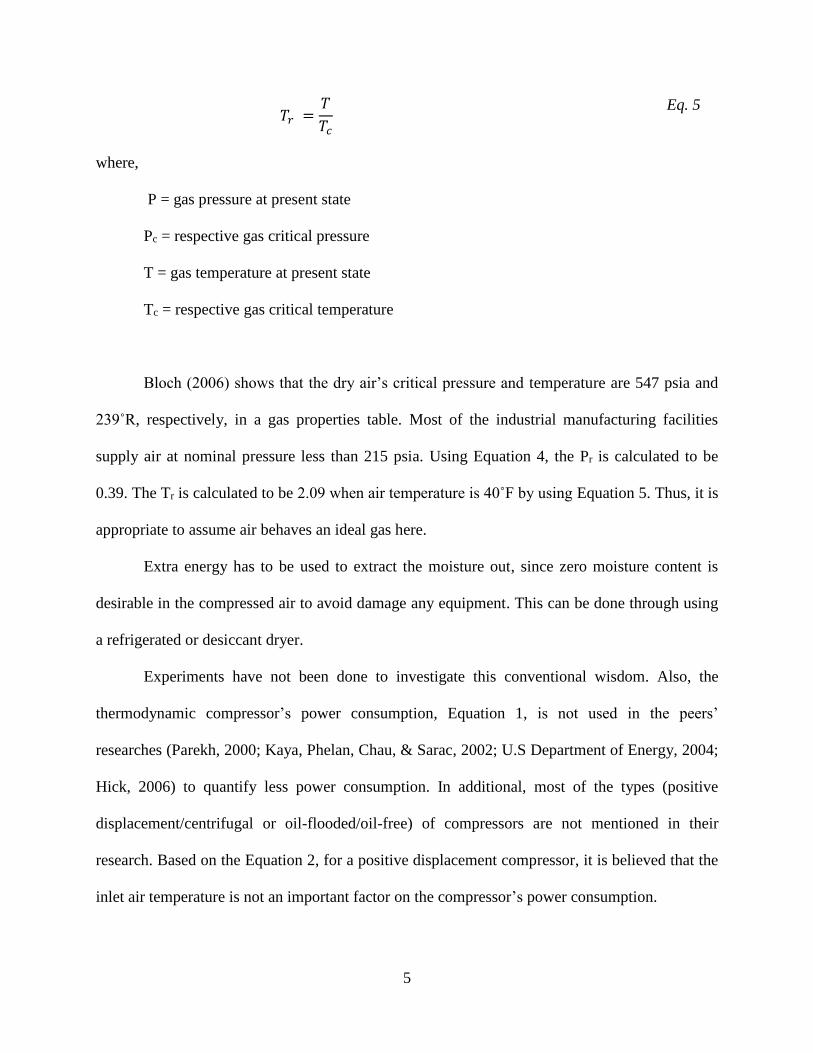
𝑇𝑟 =𝑇

𝑇𝑐

Eq. 5

where,

P = gas pressure at present state

Pc = respective gas critical pressure

T = gas temperature at present state

Tc = respective gas critical temperature

Bloch (2006) shows that the dry air’s critical pressure and temperature are 547 psia and

239˚R, respectively, in a gas properties table. Most of the industrial manufacturing facilities

supply air at nominal pressure less than 215 psia. Using Equation 4, the Pr is calculated to be

0.39. The Tr is calculated to be 2.09 when air temperature is 40˚F by using Equation 5. Thus, it is

appropriate to assume air behaves an ideal gas here.

Extra energy has to be used to extract the moisture out, since zero moisture content is

desirable in the compressed air to avoid damage any equipment. This can be done through using

a refrigerated or desiccant dryer.

Experiments have not been done to investigate this conventional wisdom. Also, the

thermodynamic compressor’s power consumption, Equation 1, is not used in the peers’

researches (Parekh, 2000; Kaya, Phelan, Chau, & Sarac, 2002; U.S Department of Energy, 2004;

Hick, 2006) to quantify less power consumption. In additional, most of the types (positive

displacement/centrifugal or oil-flooded/oil-free) of compressors are not mentioned in their

research. Based on the Equation 2, for a positive displacement compressor, it is believed that the

inlet air temperature is not an important factor on the compressor’s power consumption.

6

1.3 Literature Review

According to the Department of Energy’s Compressed Air Tip Sheet (2004), inlet air

temperature has only a slight effect on the oil-flooded, rotary screw compressors due to the oil

temperature, which is relatively high, being dominant when it mixes with the incoming air. In

other words, the incoming air still stays fairly high temperature, which is less dense, even though

the compressor breathes in cooler air; thus, there are less power reduction compared to an oil-

free compressor. Similarly, Hunt (2012) concluded from his experiment that the inlet air

temperature has a less significant effect on an oil-flooded rotary screw compressor since the

intake air temperature is dominated by the oil injected temperature. This conclusion is mainly

based on the weak R2 value on a graph plotting the measured power against the inlet air

temperature.

In the Handbook of Mechanical Engineering Calculations (Hicks, 2006), a calculation is

shown that breathing in outside air results in a savings of 7.32% of the compressor power. This

result assumes that the average outdoor temperature is 50 ˚F, whereas the average indoor

temperature is 90 ˚F. Furthermore, the required intake volume, Iindoor, to deliver a constant air

flow rate (��) at indoor temperature can be calculated as follows: Iindoor = �� x (density of air at 70

˚F / density of air at 90 ˚F). On the other hand, the required intake volume, Ioutoor, to deliver a

constant air flow rate at outdoor temperature can be calculated as follows: Ioutoor = �� x (density of

air at 70 ˚F / density of air at 50 ˚F). The power saving is the difference between Ioutoor and Iindoor.

The difference then divided by the maximum among both results in the power saving (%). A

combined equation of the above is shown below (Hicks, 2006).

𝑃𝑠 =

𝜌70˚F

𝜌90˚F−

𝜌70˚F

𝜌50˚F𝜌70˚F

𝜌90˚F

× 100

Eq. 6

7

where,

Ps = power saving in percentage

𝜌70˚F = density of air at 70 ˚F,

𝜌90˚F = density of air at 90 ˚F

𝜌50˚F = density of air at 50 ˚F

Furthermore, based on the Equation 6, Hicks (2006) concluded that it is more economical

to locate any type of air compressor, including the positive displacement and centrifugal, outside

the building due to the lower average ambient temperature. A similar calculation is also shown in

other research papers. The fraction of the energy saving, WR, is estimated as follows (Kaya et al.,

2002).

𝑊𝑅 =(𝑇𝑖𝑛𝑑𝑜𝑜𝑟 − 𝑇𝑜𝑢𝑡𝑑𝑜𝑜𝑟)

(𝑇𝑖𝑛𝑑𝑜𝑜𝑟 + 273)

Eq. 7

where,

Tindoor = indoor temperature in ˚C

Toutdoor = outdoor temperature in ˚C

Kaya et al. (2002) also advises that if the air compressor is located inside the building,

then feed outside air into the compressor through a duct. In both Equation 6 and Equation 7, it is

noted that these calculations are solely based on the air properties. The thermodynamics relation

is not illustrated.

Parekh (2000) conducted a “what if” analysis in a paper mill by modeling the facility’s

compressed air system with the aid of a software tool. Based on this project analysis, a few rules

of thumb were developed. One of them is every 10 ˚F temperature reduction in the inlet will

8

results in 1.9% energy savings. The explanation of this is the cooler air has higher density which

can supply more compressed air. Therefore, the operating time of the compressor is reduced.

Besides this, the results show the inlet relative humidity air has fairly low effect on the amount of

dry compressed air. More specifically, 100% relative humidity in the air results in dry air

reduction of 5.01%. Moreover, all compressors in the analysis are positive displacement, and a

few of them are discovered to be oil-flooded.

Although there is little literature on the effect of inlet air temperature on rotary screw

compressor performance, several authors note that cooler air temperature will reduce power

requirements for centrifugal compressors. Kakaras, Doukelis, & Karellas (2004) states that for a

gas turbine plant, higher inlet air temperature will result in higher specific compressor work

which reduces the power output. Besides this, the higher air temperature, which results in less

dense air, causes less mass flow rate which further reduces the power output. This conclude that,

in general, for every 10 ˚C of inlet air temperature increase, the power output will be reduced

between 6% and 10%. Simultaneously, the specific compressor work increases between 1.5%

and 4%. More specifically, Kakaras et al. (2004) reported simulation results on a simple gas

turbine cycle in which the power output and efficiency of the cycle dropped as much as 14.48%

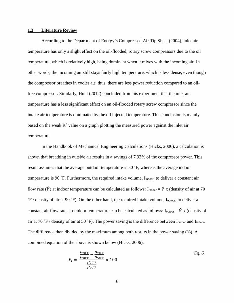
and 1.66 % at 40 ˚C with respect to ISO standard conditions (15˚C). Figure 1 depicts the

simulation result from power output and efficiency versus various ambient temperatures.

In another study with centrifugal compressors, Ravi Kumar, Rama Krishna, & Sita Rama

Raju (2007) state that cooling the compressor’s inlet air temperature will increase the air mass

flowing into the system; thereby, increases the net power output.

9

Figure 1. Power output & efficiency versus varying inlet air temperature (Kakaras et al., 2004).

In a recent study of heat transfer in screw compressors, Stosic (2015) developed detailed

CFD models of fluid flow and heat transfer in screw machines. He concludes that, since heat

dissipation from the compressed fluid to the machine is less than 1% of the power input (most of

the heat is dissipated in the after-cooler), screw compressor performance is not significantly

affected by this exchange; however, the compression process created a non-uniform three

dimensional temperature field that can deteriorate the machine’s components. He also explains

that the heat transfer is small because of the actual compression process occurs near the working

chamber discharge port where the area enclosing the compressed fluid volume is small, and the

heat transfer coefficient between the fluid and rotors is low.

Chukanova, Stosic, Kovacevic, & Dhunput (2012) studied lubrication effects on start-up

of rotary screw compressors. They found that the compressed fluid’s extreme temperature has a

direct contact with rotors may cause deterioration during the start-up mode when the screws lack

lubrication. More specifically, their experimental results show that, for a completely dry screw

3500

3700

3900

4100

4300

4500

4700

25.5

26

26.5

27

27.5

28

28.5

0 5 10 15 20 25 30 35 40

Po

wer

Ou

tpu

t (k

W)

Effi

cien

cy (

%)

T (˚C)

ISO Conditions

10

compressor, when the compressor is starting up, the compressed fluid’s temperature does not

start dropping after 8 seconds due to the inadequate pressure in the sump. A certain pressure in

sump forces the oil flows into the screw for cooling.

1.4 Design of Experiment

In the E-Handbook of Statistical Method (NIST/SEMATECH, 2013), the Design of

Experiments (DOE) is defined as an efficient method to investigate the significant impact of each

factor on the output variables. One of the DOEs is full factorial designs in two levels. The two

levels are designated to be +1 as the highest setting and -1 as the lowest setting. These highest

and lowest values can be normalized through the following equation:

𝑥𝑛𝑜𝑟𝑚𝑎𝑙𝑖𝑧𝑒𝑑 = (2𝑥𝑚𝑒𝑎𝑠 − 𝑥ℎ𝑖𝑔ℎ − 𝑥𝑙𝑜𝑤)

(𝑥ℎ𝑖𝑔ℎ − 𝑥𝑙𝑜𝑤)

Eq. 8

where,

xmeas = measured value

xhigh = the highest measured value

xlow = the lowest measured value

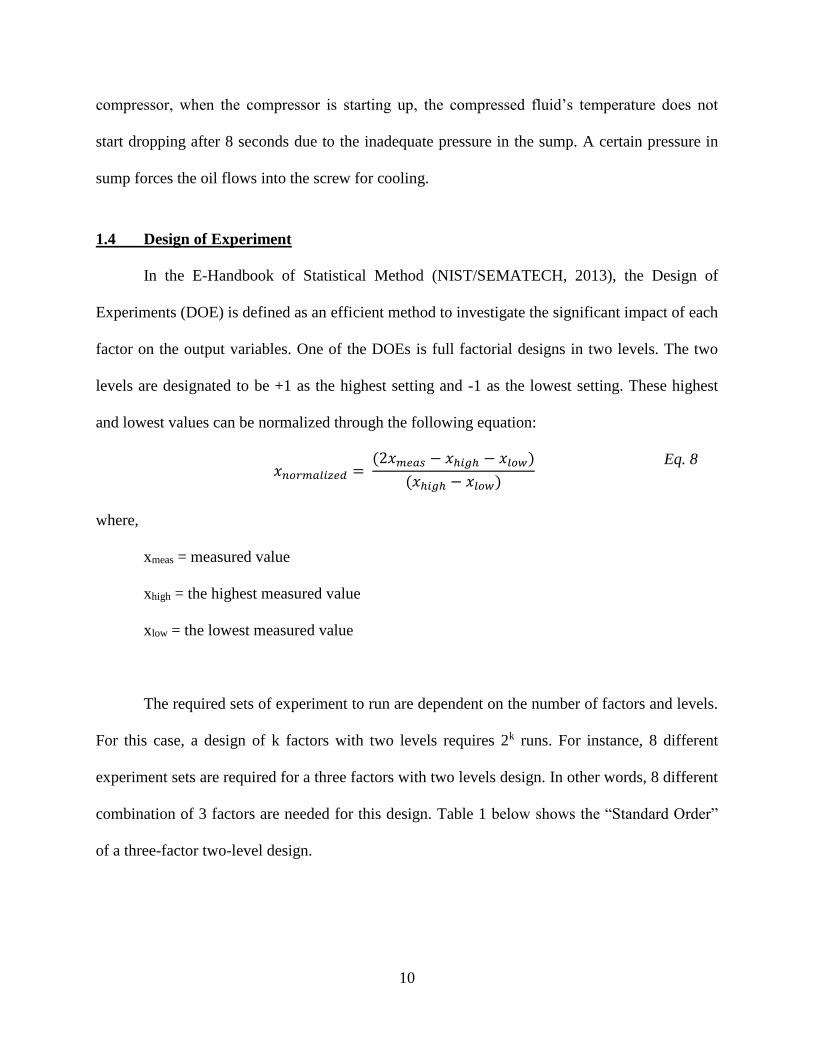
The required sets of experiment to run are dependent on the number of factors and levels.

For this case, a design of k factors with two levels requires 2k runs. For instance, 8 different

experiment sets are required for a three factors with two levels design. In other words, 8 different

combination of 3 factors are needed for this design. Table 1 below shows the “Standard Order”

of a three-factor two-level design.

11

Table 1. 2k design “Standard Order” combination (NIST/SEMATECH, 2013).

X1 X2 X3

1 -1 -1 -1

2 1 -1 -1

3 -1 1 -1

4 1 1 -1

5 -1 -1 1

6 1 -1 1

7 -1 1 1

8 1 1 1

Figure 2 is a graphical way to show the different combination of all three factors with two

levels. The arrows indicate the increase in the setting, and the number in each corner represents

each experiment set from the “Standard Order” design table.

Figure 2. Graphical representation of a 2k design (NIST/SEMATECH, 2013).

In order to determine the main effects and interactions on the dependent variable, a larger

matrix needed to be developed. A full model matrix of a 23 design is shown below in Table 2.

The determination of + or – in the column of the each interaction is the multiplication of both

corresponding columns in each row. For instance, the +1 of X1*X2 at row 1 is the multiplication

of +1 of X1 and -1 of X2 at row 1.

12

Table 2. Full model matrix of a 23 design, (NIST/SEMATECH, 2013).

In order to determine the significant impact of each variable and interactions, for a 23

design, a linear model is shown below, fitting them to the measured dependent variable (Y)

(NIST/SEMATECH, 2013).

𝑌 = 𝛼0 + 𝛼1𝑥1 + 𝛼2𝑥2 + 𝛼3𝑥3 + 𝛼4𝑥1𝑥2 + 𝛼5𝑥1𝑥3 + 𝛼6𝑥2𝑥3

+ 𝛼7𝑥1𝑥2𝑥3

Eq. 9

All the constant alphas, α, can be estimated by inversing the design’s matrix and multiply

by the corresponding measured outputs. NIST/SEMATECH (2013) also explains that

orthogonality property is important in this factorial design experiment. The orthogonality

property contains all columns (vectors) are orthogonal to each other: two vectors are orthogonal

if the sum of product of their corresponding element is zero, and the sum of each column is zero.

The orthogonality property illustrates the estimated main effects are independent of the

interactions.

I X1 X2 X1 X2 X3 X1 X3 X2 X3 X1 X2 X3

1 -1 -1 1 -1 1 1 -1

1 1 -1 -1 -1 -1 1 1

1 -1 1 -1 -1 1 -1 1

1 1 1 1 -1 -1 -1 -1

1 -1 -1 1 1 -1 -1 1

1 1 -1 -1 1 1 -1 -1

1 -1 1 -1 1 -1 1 -1

1 1 1 1 1 1 1 1

13

CHAPTER 2: AIR COMPRESSOR CHARACTERISTIC

In this chapter, rotary screws, reciprocating, and centrifugal compressors are discussed

followed by the thermodynamic compression process. Load/unload and modulating with

unloading control schemes are presented. Lastly, volumetric flow rate varies at different

condition is explained.

2.1 Types of Air Compressor

There are two different classes of air compressor: (1) centrifugal and (2) positive

displacement. A centrifugal class compressor has a rotating impeller that intakes air and converts

the kinetic energy into pressure energy. On the other hand, positive displacement compressor

compresses air by shrinking down a constant volume into a smaller volume while pressure is

increased. There are different types of positive displacement compressor–(1) rotary screw and

(2) reciprocating compressor. A rotary screw compressor typically is composed of two helical

meshing rotors whereas the reciprocating compressor is composed of a crank-shaft piston in a

cylinder. These compressors can be lubricant-injected or lubricant-free. The main purpose of

injecting lubricant into the compressor is to extract heat out, seal clearances, and reduce internal

component wear. Stosic (2015) states that for a single stage oil-free compressor, the fluid cannot

be compressed to as high as an oil-lubricated compressor due to the extreme fluid temperature

(fluid is not cooled with lubricant) can damage the rotors and housings. A typical compression

process for an oil-flooded positive displacement compressor is described as follows:

(1) Atmospheric air is breathed in through the suction port

14

(2) Simultaneously, oil is injected to mix with intake air due to the pressure difference

between the sump and compression chamber. The oil lubricates the mechanical

components and seals the clearance.

(3) During the compression, air temperature and pressure increases, and the oil extracts

heat from the air simultaneously.

(4) The mixture of air and oil is separated in an oil-separator.

(5) The compressed air and hot oil are cooled down through a heat exchanger.

(6) The cool compressed air leaves to the plant while the cool oil is injected back to the

compressor for another compression.

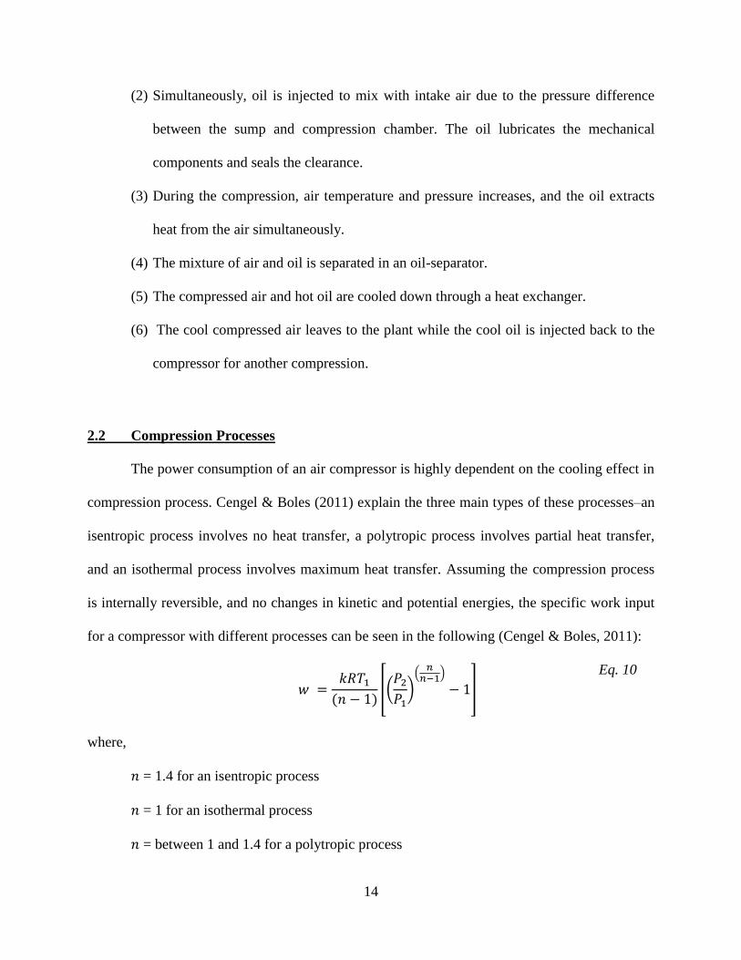
2.2 Compression Processes

The power consumption of an air compressor is highly dependent on the cooling effect in

compression process. Cengel & Boles (2011) explain the three main types of these processes–an

isentropic process involves no heat transfer, a polytropic process involves partial heat transfer,

and an isothermal process involves maximum heat transfer. Assuming the compression process

is internally reversible, and no changes in kinetic and potential energies, the specific work input

for a compressor with different processes can be seen in the following (Cengel & Boles, 2011):

𝑤 =𝑘𝑅𝑇1

(𝑛 − 1)[(

𝑃2

𝑃1)

(𝑛

𝑛−1)

− 1]

Eq. 10

where,

𝑛 = 1.4 for an isentropic process

𝑛 = 1 for an isothermal process

𝑛 = between 1 and 1.4 for a polytropic process

15

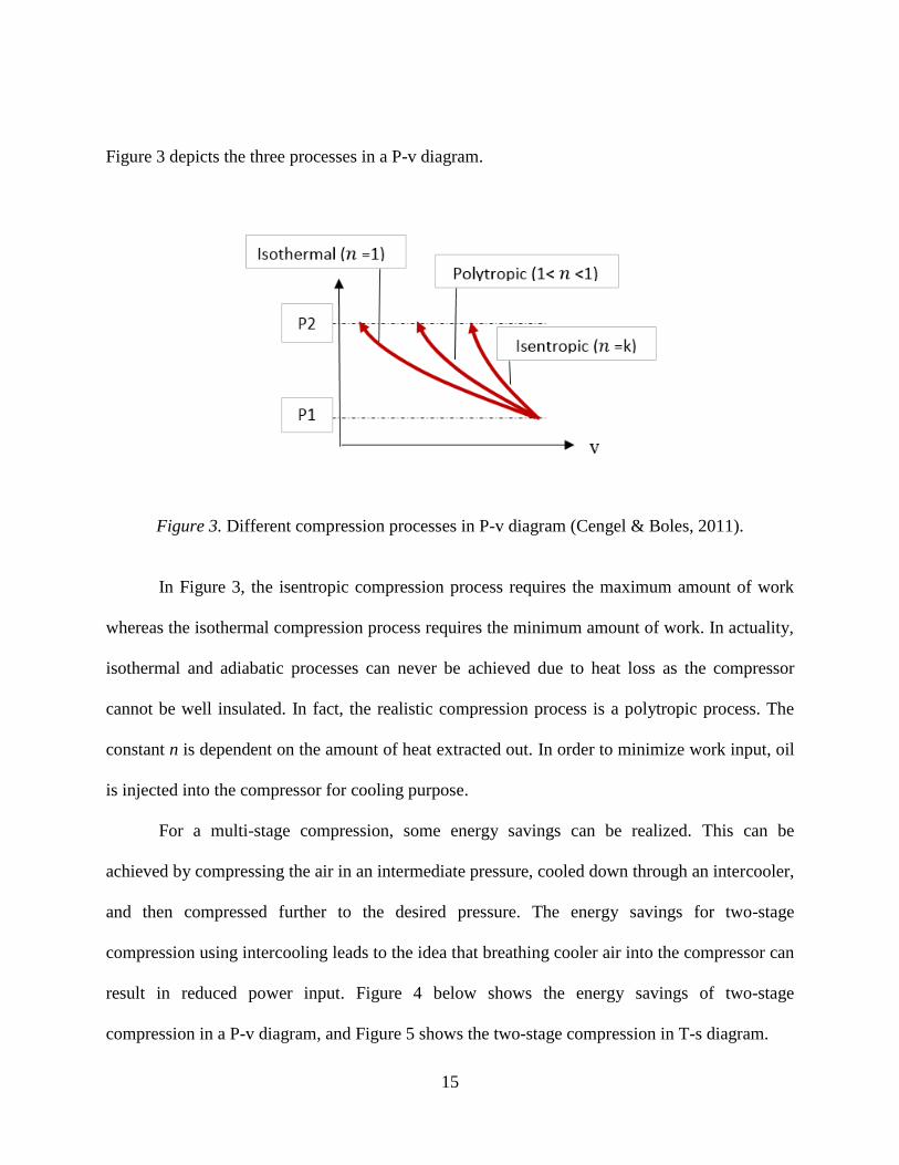
Figure 3 depicts the three processes in a P-v diagram.

Figure 3. Different compression processes in P-v diagram (Cengel & Boles, 2011).

In Figure 3, the isentropic compression process requires the maximum amount of work

whereas the isothermal compression process requires the minimum amount of work. In actuality,

isothermal and adiabatic processes can never be achieved due to heat loss as the compressor

cannot be well insulated. In fact, the realistic compression process is a polytropic process. The

constant n is dependent on the amount of heat extracted out. In order to minimize work input, oil

is injected into the compressor for cooling purpose.

For a multi-stage compression, some energy savings can be realized. This can be

achieved by compressing the air in an intermediate pressure, cooled down through an intercooler,

and then compressed further to the desired pressure. The energy savings for two-stage

compression using intercooling leads to the idea that breathing cooler air into the compressor can

result in reduced power input. Figure 4 below shows the energy savings of two-stage

compression in a P-v diagram, and Figure 5 shows the two-stage compression in T-s diagram.

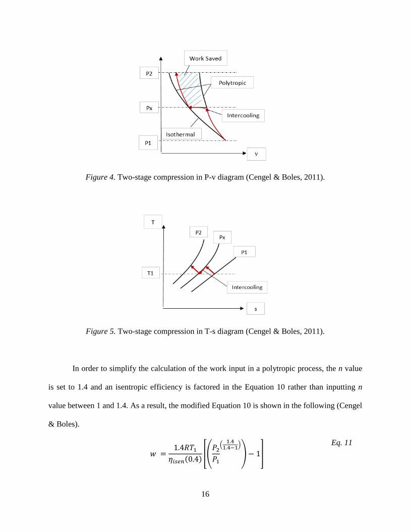
16

Figure 4. Two-stage compression in P-v diagram (Cengel & Boles, 2011).

Figure 5. Two-stage compression in T-s diagram (Cengel & Boles, 2011).

In order to simplify the calculation of the work input in a polytropic process, the n value

is set to 1.4 and an isentropic efficiency is factored in the Equation 10 rather than inputting n

value between 1 and 1.4. As a result, the modified Equation 10 is shown in the following (Cengel

& Boles).

𝑤 =1.4𝑅𝑇1

𝜂𝑖𝑠𝑒𝑛(0.4)[(

𝑃2

𝑃1

(1.4

1.4−1)

) − 1]

Eq. 11

17

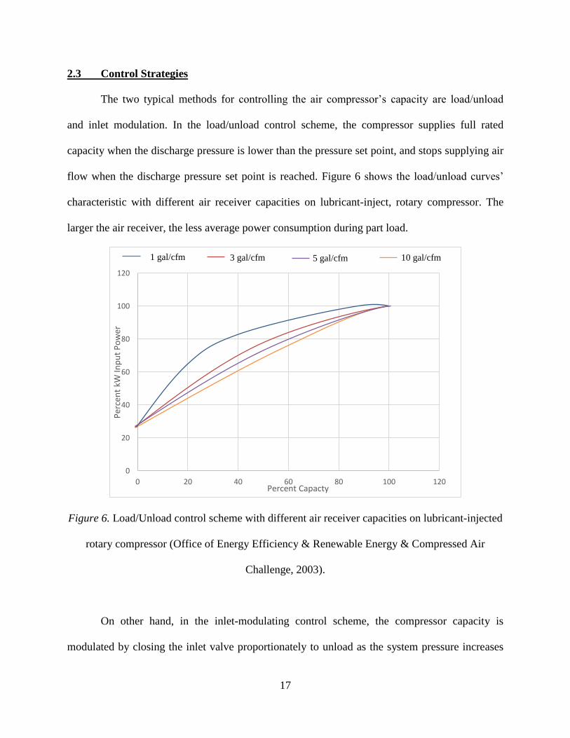
2.3 Control Strategies

The two typical methods for controlling the air compressor’s capacity are load/unload

and inlet modulation. In the load/unload control scheme, the compressor supplies full rated

capacity when the discharge pressure is lower than the pressure set point, and stops supplying air

flow when the discharge pressure set point is reached. Figure 6 shows the load/unload curves’

characteristic with different air receiver capacities on lubricant-inject, rotary compressor. The

larger the air receiver, the less average power consumption during part load.

Figure 6. Load/Unload control scheme with different air receiver capacities on lubricant-injected

rotary compressor (Office of Energy Efficiency & Renewable Energy & Compressed Air

Challenge, 2003).

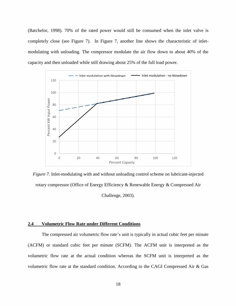
On other hand, in the inlet-modulating control scheme, the compressor capacity is

modulated by closing the inlet valve proportionately to unload as the system pressure increases

0

20

40

60

80

100

120

0 20 40 60 80 100 120

Per

cen

t kW

Inp

ut

Po

wer

Percent Capacty

1 gal/cfm 3 gal/cfm 5 gal/cfm 10 gal/cfm

18

(Batchelor, 1998). 70% of the rated power would still be consumed when the inlet valve is

completely close (see Figure 7). In Figure 7, another line shows the characteristic of inlet-

modulating with unloading. The compressor modulate the air flow down to about 40% of the

capacity and then unloaded while still drawing about 25% of the full load power.

Figure 7. Inlet-modulating with and without unloading control scheme on lubricant-injected

rotary compressor (Office of Energy Efficiency & Renewable Energy & Compressed Air

Challenge, 2003).

2.4 Volumetric Flow Rate under Different Conditions

The compressed air volumetric flow rate’s unit is typically in actual cubic feet per minute

(ACFM) or standard cubic feet per minute (SCFM). The ACFM unit is interpreted as the

volumetric flow rate at the actual condition whereas the SCFM unit is interpreted as the

volumetric flow rate at the standard condition. According to the CAGI Compressed Air & Gas

0

20

40

60

80

100

120

0 20 40 60 80 100 120

Per

cen

t kW

Inp

ut

Po

wer

Percent Capacty

Inlet modulation with blowdown Inlet modulation - no blowdown

19

Institute (2012), the standard condition is defined as the ambient at 68˚F, 14.5 psia, and 0%

relative humidity. Furthermore, an equation for converting from SCFM to ACFM is illustrated

below (CAGI Compressed Air & Gas Institute, 2012).

𝐴𝐶𝐹𝑀 = 𝑆𝐶𝐹𝑀 × [𝑃𝑠

𝑃𝑎 − (𝑝𝑝𝑚 × 𝑅𝐻)] ×

(𝑇𝑎 + 460)

(𝑇𝑠 + 460)

Eq. 12

where,

Ps = standard pressure, psia (CAGI & ISO use 14.5 psia)

Pa = atmospheric pressure, psia

ppm = partial pressure of moisture at atmospheric temperature, psia

RH = relative humidity, %

Ta = atmospheric temperature, ˚F

Ts = standard temperature, ˚F (CAGI & ISO use 68˚F)

The ppm also can be known as the saturated vapor pressure at the actual temperature.

According to the National Weather Service Weather Forecast Office (2014), the saturated vapor

pressure can be estimated as follows:

𝑒𝑠 = 6.11 × 10(

7.5𝑇𝑒237.3+𝑇𝑒

)

Eq. 13

where,

𝑒𝑠 = saturated vapor pressure in milibar.

Te = temperature in ˚C

In the Equation 12, it is noted that the air temperature plays a significant role in

converting SCFM to ACFM at atmospheric pressure. Thus, as the air temperature increases, the

flow rate in atmosphere increases.

20

CHAPTER 3: EXPERIMENT

A controlled environment was set up for this experiment. Three DOE models are

developed. There are 3 factors with 2 levels on compressor power (3F2L–CP), 2 factors with 2

levels on compressor power (2F2L–CP), and 2 factors with 2 levels on inlet oil temperature

(2F2L–OIT). An air demand simulator was built to control the air demand, and different ambient

temperatures used to vary the inlet air temperature. Therefore, the relationship between the

power consumption, produced air flow, and inlet air temperature of the compressor can be

investigated.

3.2 Objective

The two main objectives of this experiment are (1) perform DOE to investigate the

significant effect of air flow rate (Vair), inlet air temperature (Tair,in) and injected oil temperature

(Toil,in) on the compressor’s power (Wmeas), and (2) determine the relationship between the

measured compressor’s power input with the inlet air temperature through using thermodynamic

analysis.

3.3 Experiment Setup

A rated 30 hp Ingersoll Rand oil-flooded, air cooled, rotary screw air compressor was

used in this experiment. The air compressor’s model, serial number, rated capacity, and

maximum operating pressure are SSR UP6-30-200, PY3415U10309, 92 acfm, and 200 psig,

respectively. Also, there was a 120 gallon air receiver underneath the compressor. The

21

compressor’s motor is three-phase and serviced with a nominal voltage of 200. This compressor

is located inside a building, Annex2, at the University of Alabama. This compressor solely

supplies compressed air to the student machine shop (next two rooms of the compressor room).

A dryer is in placed after the compressor and followed by a pressure regulator. A 1 inch, type L,

copper piping line is used throughout the compressed air system. The control strategy of the

compressor is a load/unload scheme. The set points of the load and unload were 125 and 135

psig, respectively. The pressure regulator decreased the high pressure air to 100 psig. In the

machine shop, compressed air is again regulated down to 95 psig through another pressure

regulator.

Four different experimental configurations were set up: (1) the original compressor

configuration, (2) original compressor configuration with an insulated flexible duct, (3) covered

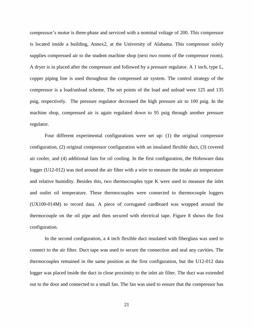
air cooler, and (4) additional fans for oil cooling. In the first configuration, the Hoboware data

logger (U12-012) was tied around the air filter with a wire to measure the intake air temperature

and relative humidity. Besides this, two thermocouples type K were used to measure the inlet

and outlet oil temperature. These thermocouples were connected to thermocouple loggers

(UX100-014M) to record data. A piece of corrugated cardboard was wrapped around the

thermocouple on the oil pipe and then secured with electrical tape. Figure 8 shows the first

configuration.

In the second configuration, a 4 inch flexible duct insulated with fiberglass was used to

connect to the air filter. Duct tape was used to secure the connection and seal any cavities. The

thermocouples remained in the same position as the first configuration, but the U12-012 data

logger was placed inside the duct in close proximity to the inlet air filter. The duct was extended

out to the door and connected to a small fan. The fan was used to ensure that the compressor has

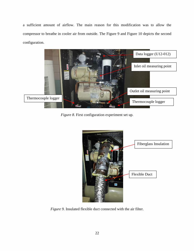
22

a sufficient amount of airflow. The main reason for this modification was to allow the

compressor to breathe in cooler air from outside. The Figure 9 and Figure 10 depicts the second

configuration.

Figure 8. First configuration experiment set up.

Figure 9. Insulated flexible duct connected with the air filter.

Data logger (U12-012)

Inlet oil measuring point

Outlet oil measuring point

Thermocouple logger Thermocouple logger

Fiberglass Insulation

Flexible Duct

23

Figure 10. Fan connected with the duct to supply air.

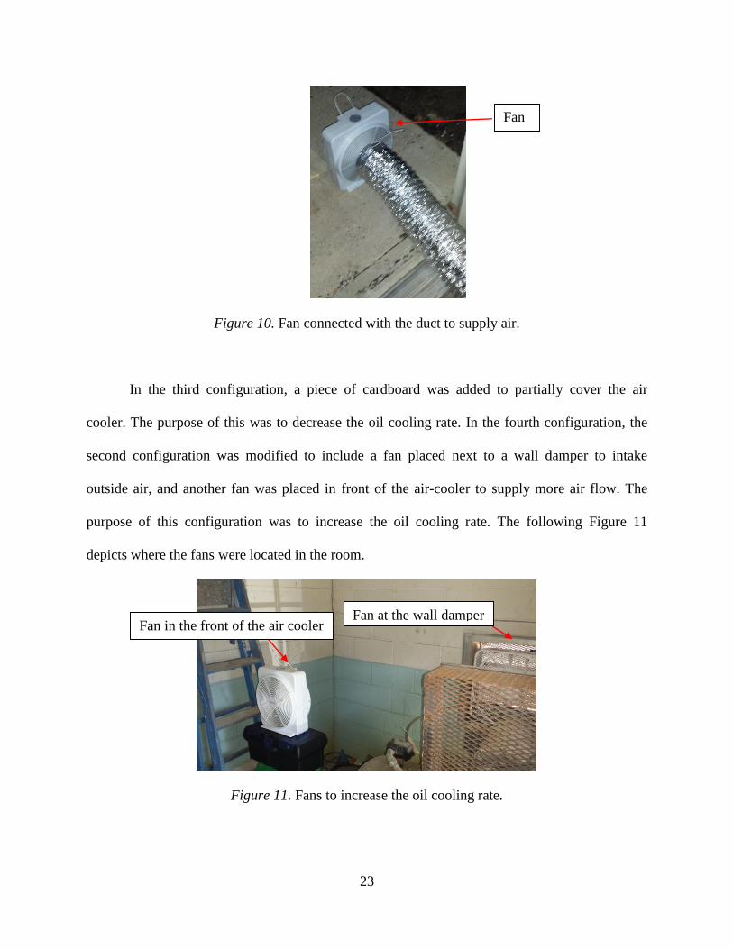
In the third configuration, a piece of cardboard was added to partially cover the air

cooler. The purpose of this was to decrease the oil cooling rate. In the fourth configuration, the

second configuration was modified to include a fan placed next to a wall damper to intake

outside air, and another fan was placed in front of the air-cooler to supply more air flow. The

purpose of this configuration was to increase the oil cooling rate. The following Figure 11

depicts where the fans were located in the room.

Figure 11. Fans to increase the oil cooling rate.

Fan

Fan at the wall damper Fan in the front of the air cooler

24

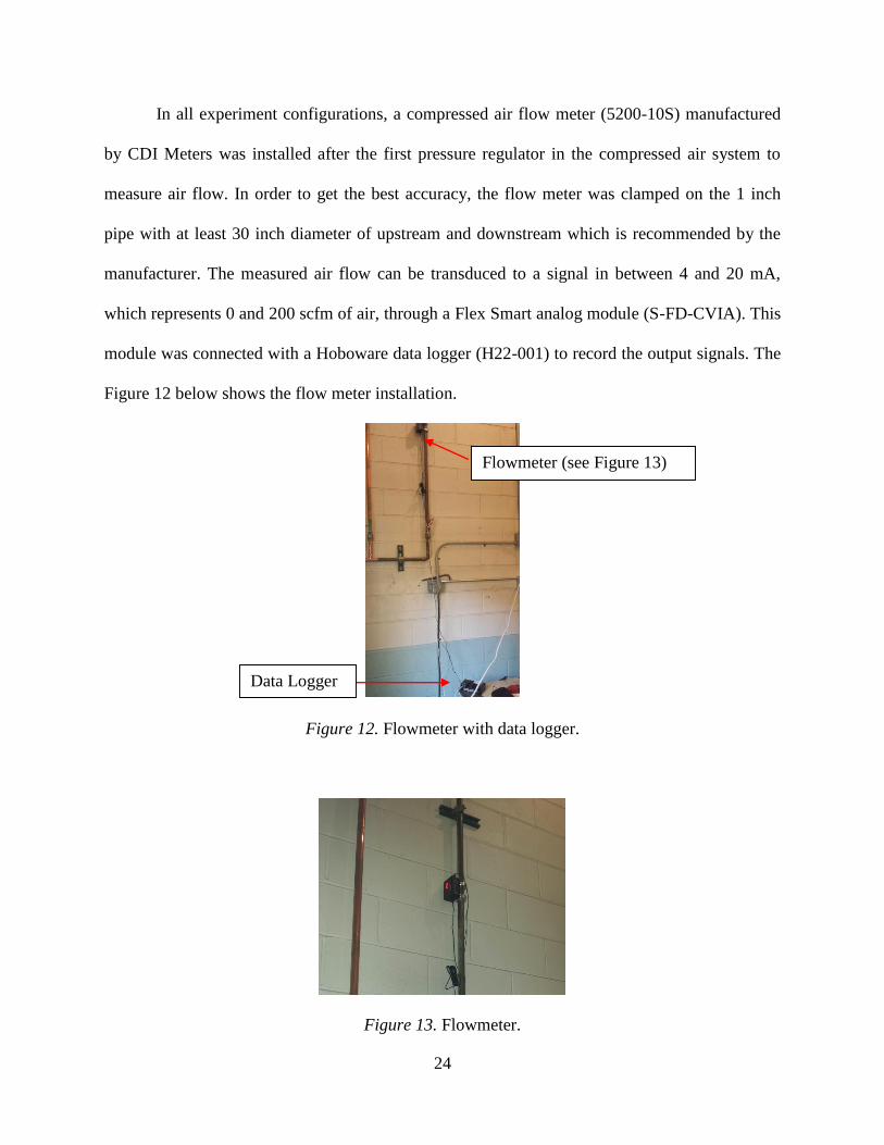
In all experiment configurations, a compressed air flow meter (5200-10S) manufactured

by CDI Meters was installed after the first pressure regulator in the compressed air system to

measure air flow. In order to get the best accuracy, the flow meter was clamped on the 1 inch

pipe with at least 30 inch diameter of upstream and downstream which is recommended by the

manufacturer. The measured air flow can be transduced to a signal in between 4 and 20 mA,

which represents 0 and 200 scfm of air, through a Flex Smart analog module (S-FD-CVIA). This

module was connected with a Hoboware data logger (H22-001) to record the output signals. The

Figure 12 below shows the flow meter installation.

Figure 12. Flowmeter with data logger.

Figure 13. Flowmeter.

Flowmeter (see Figure 13)

Data Logger

25

Next, a rated 300 amperage power transducer (H8044-0400-3) was used to measure the

power draw for the compressor. More specifically, each clamp was clamped to each phase leg.

All three clamps were connected to a Flex Smart Analog module and a H22-001 data logger for

data recording purpose. The Figure 14 shows the power transducer was clamped in the electrical

circuit cabinet.

Figure 14. Power transducer and data logger installation in the power cabinet.

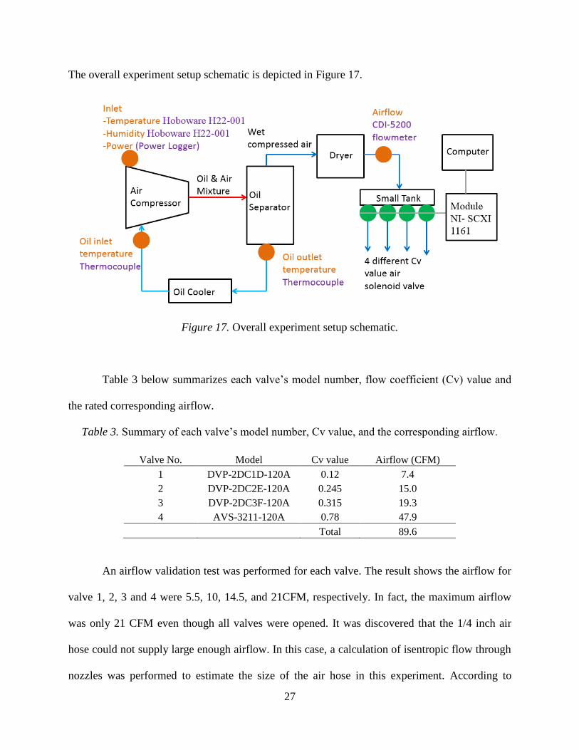
In the student machine shop, an air demand simulating system was built in order to

control the air demand. This simulating system consists of a computer, chassis (SCXI 1000),

module (SCXI 1161), 2 gallon tank, 4 solenoid valves, and power supply adapter. LabView

software was used for the programming in the simulating system. Figure 15 depicts the air

demand simulating system.

More specifically, the Chassis and module were both purchased from the National

Instruments. A graduated student, Hamid Najafi, from the Department of Mechanical

Engineering of the University of Alabama, developed a programming code to run the simulating

system using the LabView software tool. The code reads an Excel file which allows the user to

specify the valves to be turned on or off for a period of time. Furthermore, the four pneumatic

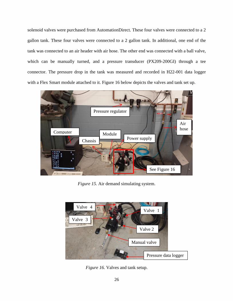
26

solenoid valves were purchased from AutomationDirect. These four valves were connected to a 2

gallon tank. These four valves were connected to a 2 gallon tank. In additional, one end of the

tank was connected to an air header with air hose. The other end was connected with a ball valve,

which can be manually turned, and a pressure transducer (PX209-200GI) through a tee

connector. The pressure drop in the tank was measured and recorded in H22-001 data logger

with a Flex Smart module attached to it. Figure 16 below depicts the valves and tank set up.

Figure 15. Air demand simulating system.

Figure 16. Valves and tank setup.

Pressure data logger

Pressure regulator

Computer

Chassis

Module Power supply

Air

hose

See Figure 16

Manual valve

Valve 2

Valve 1

Valve 2 Valve 3

Valve 2

Valve 4

Valve 2

27

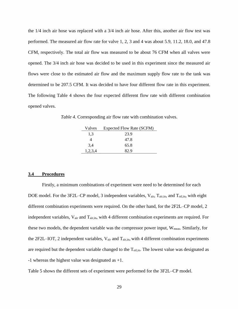
The overall experiment setup schematic is depicted in Figure 17.

Figure 17. Overall experiment setup schematic.

Table 3 below summarizes each valve’s model number, flow coefficient (Cv) value and

the rated corresponding airflow.

Table 3. Summary of each valve’s model number, Cv value, and the corresponding airflow.

Valve No. Model Cv value Airflow (CFM)

1 DVP-2DC1D-120A 0.12 7.4

2 DVP-2DC2E-120A 0.245 15.0

3 DVP-2DC3F-120A 0.315 19.3

4 AVS-3211-120A 0.78 47.9

Total 89.6

An airflow validation test was performed for each valve. The result shows the airflow for

valve 1, 2, 3 and 4 were 5.5, 10, 14.5, and 21CFM, respectively. In fact, the maximum airflow

was only 21 CFM even though all valves were opened. It was discovered that the 1/4 inch air

hose could not supply large enough airflow. In this case, a calculation of isentropic flow through

nozzles was performed to estimate the size of the air hose in this experiment. According to

28

Cengel & Boles (2011), the Mach number is defined as the ratio of speed of a fluid to the speed

of sound of the same fluid and can be assumed as 1 when the maximum mass flow rate at the

throat is calculated. Since the compressed air is in standard condition, the air temperature is

assumed to be 68 °F. In steady state, the maximum volumetric flowrate in the 1/4 inch air hose

was calculated as follows (Cengel & Boles, 2011).

��𝑚𝑎𝑥 = 𝐴 × 𝑀𝑎 × √𝑘 × 𝑅 × 𝑇 × 𝑔𝑐 × 𝑘1

= 0.0003409𝑓𝑡2 × 1 × √1.4 × 53.34𝑓𝑡−𝑙𝑏𝑓

𝑙𝑏𝑚−°𝑅× 529 °R × 32.174

𝑓𝑡−𝑙𝑏𝑚

𝑙𝑏𝑓−𝑠2 × 60 𝑠𝑒𝑐𝑜𝑛𝑑𝑠

1 𝑚𝑖𝑛𝑢𝑡𝑒

= 23.1 CFM

where,

��𝑚𝑎𝑥 = maximum volumetric air flow rate in the air hose

𝐴 = cross section area of the air hose

Ma = Mach number

k = isentropic coefficient

R = universal air constant

T = compressed air temperature

gc = specific gravity

k1 = conversion factor

The determined maximum air flow rate in the 1/4 inch air hose was only 23.1 CFM

which is close to the measured air flow rate (21 CFM). In order to allow each valve to release its

estimated air flow rate, the above equation was calculated again with a different air hose size

which was 3/4 inch diameter. The maximum flow rate was determined to be 207.5 CFM in the

3/4 inch air hose which exceed the desired total air flow from all valves (89.6 CFM). Therefore,

29

the 1/4 inch air hose was replaced with a 3/4 inch air hose. After this, another air flow test was

performed. The measured air flow rate for valve 1, 2, 3 and 4 was about 5.9, 11.2, 18.0, and 47.8

CFM, respectively. The total air flow was measured to be about 76 CFM when all valves were

opened. The 3/4 inch air hose was decided to be used in this experiment since the measured air

flows were close to the estimated air flow and the maximum supply flow rate to the tank was

determined to be 207.5 CFM. It was decided to have four different flow rate in this experiment.

The following Table 4 shows the four expected different flow rate with different combination

opened valves.

Table 4. Corresponding air flow rate with combination valves.

Valves Expected Flow Rate (SCFM)

1,3 23.9

4 47.8

3,4 65.8

1,2,3,4 82.9

3.4 Procedures

Firstly, a minimum combinations of experiment were need to be determined for each

DOE model. For the 3F2L–CP model, 3 independent variables, Vair, Tair,in, and Toil,in, with eight

different combination experiments were required. On the other hand, for the 2F2L–CP model, 2

independent variables, Vair and Tair,in, with 4 different combination experiments are required. For

these two models, the dependent variable was the compressor power input, Wmeas. Similarly, for

the 2F2L–IOT, 2 independent variables, Vair and Tair,in, with 4 different combination experiments

are required but the dependent variable changed to the Toil,in. The lowest value was designated as

-1 whereas the highest value was designated as +1.

Table 5 shows the different sets of experiment were performed for the 3F2L–CP model.

30

Table 5. 3F2L–CP model.

Experiment set Vair Tair,in Toil,in

1 + + +

2 – + +

3 + – +

4 – – +

5 + + –

6 – + –

7 + – –

8 – – –

The Table 6 below shows the different sets of experiments that were performed for the

2F2L–CP and 2F2L–IOT model.

Table 6. 2F2L–CP and 2F2L–IOT model

Experiment set Vair Tair,in

1 + +

2 – +

3 + –

4 – –

The Vair can be controlled by using the air demand simulator. For every set of

experiments, the compressor power was measured and four different air flow rates were set in an

interval of 30 minutes. There were about 23 SCFM (25% loaded), 48 SCFM (52% loaded), 63

SCFM (68% loaded), and 75 SCFM (82% loaded). A test run was performed on the first

experimental configuration on February 5th. Data were collected to ensure the proper set up and

functional instruments.

For the first two set of experiments, the first experimental configuration was set up. The

compressor’s door room was shut completely and the experiments were performed in the

February 5th and 8th. Furthermore, the second experimental configuration, without extending the

flexible duct to outdoor, was set up to collect more data for the first two sets on March 8th. For

31

the 3rd and 4th set of experiments, the second experimental configuration was set up and

performed during the cool nights, March 5th and 6th, with an opened door. The air cooler on the

side was covered about half of the area in order to restrict the air flow for oil cooling; thus, the

Toil,in was expected to increase. For the 5th and 6th experiments, the fourth experimental

configuration was set up with some slight modification. More specifically, instead of extending

the flexible duct out to the door, the insulated flexible duct was rearranged to breathe in hot air as

shown in the following Figure 18.

Figure 18. Fourth configuration with slight modification.

The original fourth experimental configuration was set up to perform the 7th and 8th set of

experiments during the cool days (February 12th and 17th) with an opened door. An additional

data was collected on February 5th.

All data were imported to Hoboware software. Then, an average is determined in that 30

minutes interval. When the air demand simulator was not programmed, the recorded data

indicates that the compressor was loaded lightly once in a while. It was observed that the

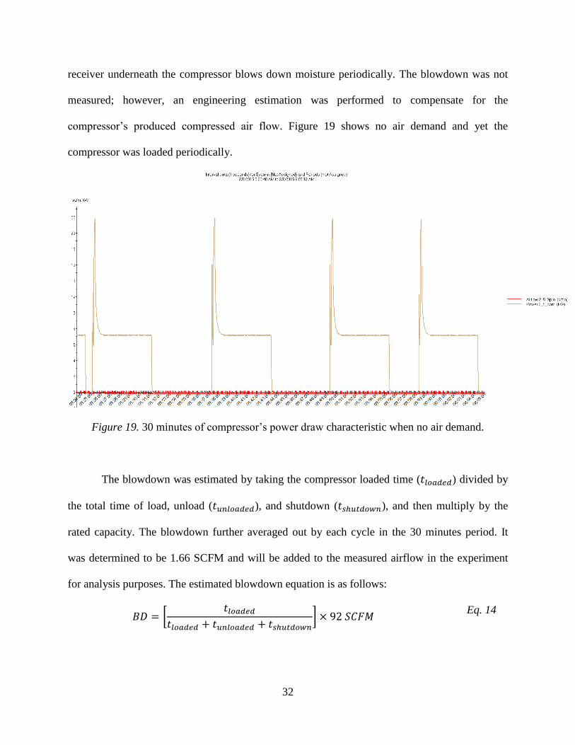
32

receiver underneath the compressor blows down moisture periodically. The blowdown was not

measured; however, an engineering estimation was performed to compensate for the

compressor’s produced compressed air flow. Figure 19 shows no air demand and yet the

compressor was loaded periodically.

Figure 19. 30 minutes of compressor’s power draw characteristic when no air demand.

The blowdown was estimated by taking the compressor loaded time (𝑡𝑙𝑜𝑎𝑑𝑒𝑑) divided by

the total time of load, unload (𝑡𝑢𝑛𝑙𝑜𝑎𝑑𝑒𝑑), and shutdown (𝑡𝑠ℎ𝑢𝑡𝑑𝑜𝑤𝑛), and then multiply by the

rated capacity. The blowdown further averaged out by each cycle in the 30 minutes period. It

was determined to be 1.66 SCFM and will be added to the measured airflow in the experiment

for analysis purposes. The estimated blowdown equation is as follows:

𝐵𝐷 = [𝑡𝑙𝑜𝑎𝑑𝑒𝑑

𝑡𝑙𝑜𝑎𝑑𝑒𝑑 + 𝑡𝑢𝑛𝑙𝑜𝑎𝑑𝑒𝑑 + 𝑡𝑠ℎ𝑢𝑡𝑑𝑜𝑤𝑛] × 92 𝑆𝐶𝐹𝑀

Eq. 14

33

3.5 Result and Discussion

3.5.1 Design of Experiment

Conventional wisdom dictates that the compressor power is highly dependent on the inlet

air temperature. Thus, the 3F2L–CP model was developed and the result will determine the

significant effect of Vair, Tair,in, and Toil,in on the compressor power. Likewise, the 2F2L–CP

model was developed by disregarding the Toil,in to investigate the effect between Vair and Tair,in on

the compressor power. There are some researchers who argue that the compressor power can be

affected by the Tair,in due to dominant of higher Toil,in. The 2F2L–IOT model was developed to

investigate the significant impact of the Tair,in and Vair on Toil,in.

3F2L–CP Model

Since the minimum and maximum values for each dependent variable could not be set

accurately, a few groups of data on each experiment set to the desired values were chosen. Then,

the average of each set was used as a representation.

Table 7 shows the chosen groups of data for each set. Table 8 shows the average data for

each dependent variable on different combination experiment, and minimum and maximum

values were determined for the 3F2L–CP model. Next, the data sets of the 3F2L–CP model were

normalized using Equation 8. Table 9 shows the normalized data. x1, x2 and x3 are defined as

Vair, Tair,in, and Toil,in, respectively. From Table 9, it is noted that some of the Tair,in and Toil,in

normalized values were not quite close to the corresponding desired value. The Toil,in in

experiment set 2 was not as high as the one in set 1. These two sets were performed during the

day time with the door closed. It is noted that the Toil,in was lower when compressing lower air

34

flow rate. The Toil,in value on experiment set 3 is close to zero which is in the middle range, and

Toil,in value on experiment set 4 is not close to the positive value.

Table 7. Group of data on each combination experiment.

Desired Measured

Experiment

number Vair

(SCFM) Tair,in

(˚F) Toil,in

(˚F) Vair

(SCFM) Tair,in

(˚F) Toil,in

(˚F) Wmeas

(kW)

1 + + + 76.9 115.0 163.6 19.32

80.5 121.4 162.3 19.73

2

– + + 24.6 116.6 150.9 12.67

26.8 121.2 146.7 13.08

3 + – +

75.4 31.4 132.8 19.38

75.7 29.4 138.9 19.41

75.8 28.7 140.6 19.44

75.9 30.8 138.4 19.41

4 – – +

23.1 33.0 123.0 12.77

22.8 33.0 120.1 12.69

23.0 31.0 122.0 12.79

22.8 31.3 119.7 12.73

5 + + –

74.7 87.6 133.1 19.29

75.0 92.3 148.2 19.36

75.1 83.0 143.2 19.23

6 – + – 23.1 89.0 122.3 12.65

23.1 91.3 132.9 12.63

7 + – – 78.1 33.0 130.6 19.72

78.0 34.4 128.1 19.71

8 – – – 25.3 34.4 115.4 13.11

25.3 34.4 116.5 13.21

Table 8. Data for 3F2L–CP model.

Vair

(SCFM) Tair,in

(˚F) Toil,in

(˚F) Vair

(SCFM) Tair,in

(˚F) Toil,in

(˚F) Wmeas

(kW)

+ + + 78.7 118.2 162.9 19.52

– + + 25.7 118.9 148.8 12.88 + – + 75.7 30.1 137.6 19.41 – – + 22.9 32.1 121.2 12.74 + + – 74.9 87.6 141.5 19.29 – + – 23.1 90.1 127.6 12.64 + – – 78.1 33.7 129.3 19.72 – – – 25.3 34.4 116.0 13.16

Max 78.7 118.9 162.9

Min 22.9 30.1 116.0

35

Table 9. 3F2L–CP model normalized data

Desired Normalized

Experiment

set Vair

(SCFM) Tair,in

(˚F) Toil,in

(˚F) Vair

(SCFM) Tair,in

(˚F) Toil,in

(˚F)

1 + + + 1.00 0.98 1.00 2 – + + -0.90 1.00 0.40 3 + – + 0.89 -1.00 -0.08 4 – – + -1.00 -0.95 -0.78 5 + + – 0.86 0.30 0.09 6 – + – -0.99 0.35 -0.50 7 + – – 0.98 -0.92 -0.43 8 – – – -0.91 -0.90 -1.00

Since the compressor is air-cooled, the Toil,in is highly dependent on the ambient

temperature. These two sets of experiment were performed during cold nights; therefore, the

Toil,in could not achieve as high as experiment set 1 and 2 even though airflow was restricted to

cool the oil by covering the oil-cooler surface. Experiment set 5 and 6 were also performed

during the cold nights because cold outside air was pulled in by a fan to cool the Toil,in. In this

case, the Tair,in could not reach as high as set 1 because air temperature was adjusted by the heat

dissipation of the compressor itself and the door was closed to decrease the heat loss from the

room. Both experiments 7 and 8 were performed during the cold night as well due to cold Toil,in

and Tair,in were needed. It was observed that the Toil,in could not achieve as low as the one in set 8

when compressing higher flow rate.

The normalized data was then constructed to a matrix form, Matrix A. The effect of each

dependent variable and variables interaction on the compressor’s power were determined. The

normalized data matrix and effect of each variable is shown in

Table 10. Another graph is shown in Figure 20 to have a better visual of each variable

effect on the compressor power.

36

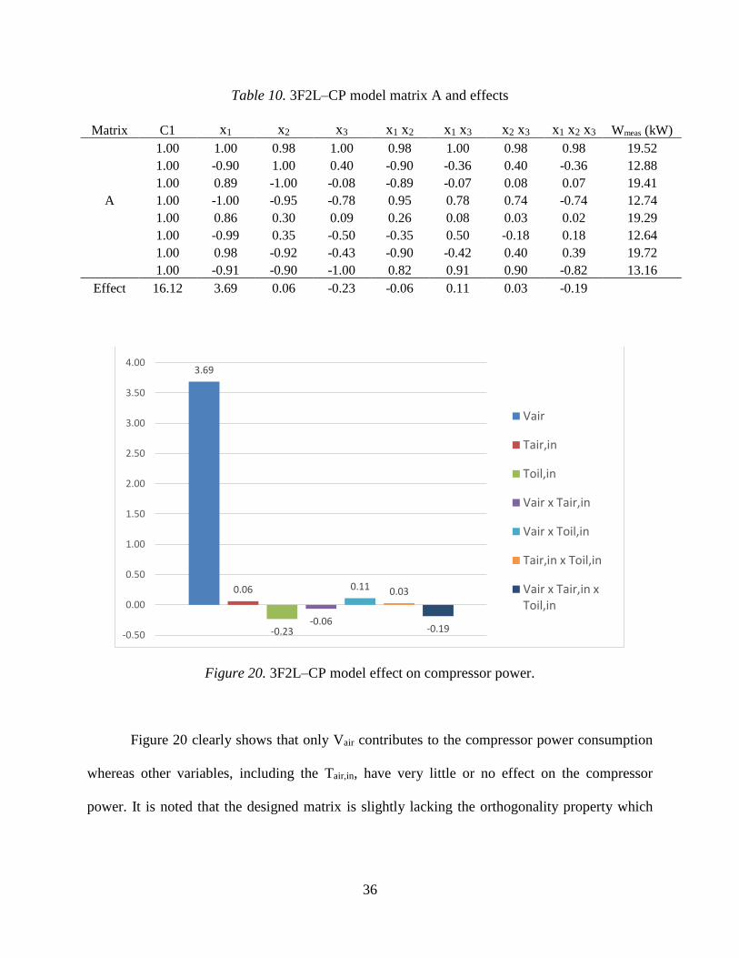
Table 10. 3F2L–CP model matrix A and effects

Matrix C1 x1 x2 x3 x1 x2 x1 x3 x2 x3 x1 x2 x3 Wmeas (kW)

1.00 1.00 0.98 1.00 0.98 1.00 0.98 0.98 19.52

1.00 -0.90 1.00 0.40 -0.90 -0.36 0.40 -0.36 12.88

1.00 0.89 -1.00 -0.08 -0.89 -0.07 0.08 0.07 19.41

A 1.00 -1.00 -0.95 -0.78 0.95 0.78 0.74 -0.74 12.74

1.00 0.86 0.30 0.09 0.26 0.08 0.03 0.02 19.29

1.00 -0.99 0.35 -0.50 -0.35 0.50 -0.18 0.18 12.64

1.00 0.98 -0.92 -0.43 -0.90 -0.42 0.40 0.39 19.72

1.00 -0.91 -0.90 -1.00 0.82 0.91 0.90 -0.82 13.16

Effect 16.12 3.69 0.06 -0.23 -0.06 0.11 0.03 -0.19

Figure 20. 3F2L–CP model effect on compressor power.

Figure 20 clearly shows that only Vair contributes to the compressor power consumption

whereas other variables, including the Tair,in, have very little or no effect on the compressor

power. It is noted that the designed matrix is slightly lacking the orthogonality property which

3.69

0.06

-0.23-0.06

0.11 0.03

-0.19-0.50

0.00

0.50

1.00

1.50

2.00

2.50

3.00

3.50

4.00

Vair

Tair,in

Toil,in

Vair x Tair,in

Vair x Toil,in

Tair,in x Toil,in

Vair x Tair,in xToil,in

37

implies the correlation between estimated main effects and interactions are not eliminated

completely. Table 11 shows the determined calculation for orthogonal property.

Table 11. 3F2L–CP Orthogonal property

Summation of

column Summation of two vectors

multiplication

x1 x2 x3 x1 x2 x1 x3 x2 x3

-0.07 -1.14 -1.3 -0.02 2.42 3.35

2F2L–CP Model

In this model, the only difference from 3F2L–CP model was the absence of Toil,in. Less

experiment sets were accounted since only two dependent variables are investigated. In fact, the

first 4 experiment sets that shown on Table 6 were used to develop this model. The following

Table 12 shows the first 4 sets data with their corresponding normalized value for Vair and Tair,in,

and new minimum and maximum values were determined.

Table 12. 2F2L–CP model normalized data

Desired Measured Normalized Experiment

set Vair

(SCFM) Tair,in

(˚F) Vair

(SCFM) Tair,in

(˚F) Vair

(SCFM) Tair,in

(˚F)

1 + + 77.1 118.2 1.00 0.98 2 – + 24.1 118.9 -0.90 1.00 3 + – 74.1 30.1 0.89 -1.00 4 – – 21.2 32.1 -1.00 -0.95

Maximum 77.1 118.9

Minimum 21.2 30.1

The normalized data was constructed in Matrix B, and the effect was determined through

the DOE method.

Table 13 shows the normalized data matrix and each effect of the variable on the compressor

power. Figure 21 shows the each variable effect on the compressor power.

38

Table 13. 3F2L–CP model matrix B and effects

Matrix C1 x1 x2 x1 x2 Wmeas (kW)

1.00 1.00 0.98 0.98 19.5

B 1.00 -0.90 1.00 -0.90 12.9

1.00 0.89 -1.00 -0.89 19.4

1.00 -1.00 -0.95 0.95 12.7

Effect 16.14 3.51 -0.12 -0.01

Figure 21. 3F2L–CP model effect on compressor power.

Similarly to the result from 3F2L–CP, only the Vair contributes to the compressor power

whereas others contribute much less or no to the compressor power. Table 14 shows that this

designed matrix has the orthogonality property; therefore, the estimated main effect is

independent of the interaction.

Table 14. 2F2L–CP Orthogonal property

Summation of

column Summation product of

two vectors

x1 x2 x1 x2

-0.01 0.03 0.15

3.51

-0.12 -0.01-0.50

0.00

0.50

1.00

1.50

2.00

2.50

3.00

3.50

4.00

Vair

Tair,in

Vair x Tair,in

39

2F2L–IOT Model

This model analysis is very similar to the 2F2L–CP model analysis. The exact same data

was used, but the dependent variable, compressor power (Wmeas), was changed to the Toil,in. Table

15 below shows the normalized data in matrix C and each effect of variable on the inlet oil

temperature. Figure 22 shows the each variable effect on the inlet oil temperature.

Table 15. 2F2L–IOT model matrix C and effects

C1 x1 x2 x1 x2 Toil,in

1.00 1.00 0.98 0.98 162.95

C 1.00 -0.90 1.00 -0.90 148.76

1.00 0.89 -1.00 -0.89 137.65

1.00 -1.00 -0.95 0.95 121.18

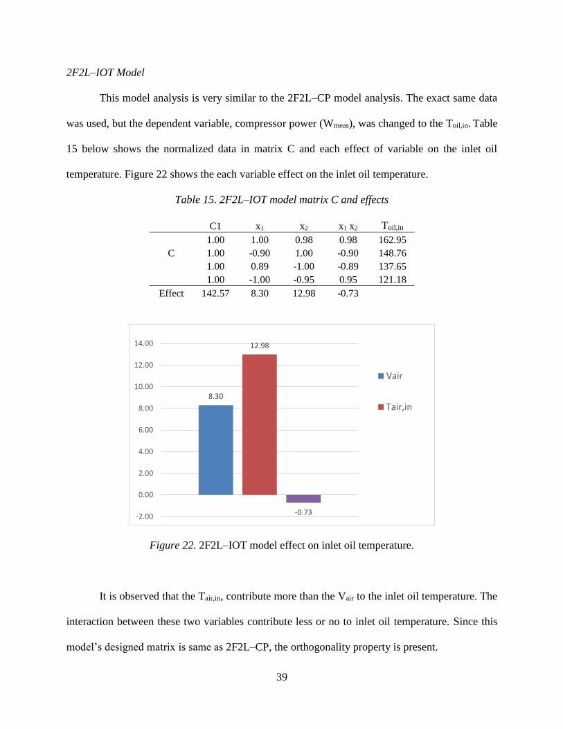
Effect 142.57 8.30 12.98 -0.73

Figure 22. 2F2L–IOT model effect on inlet oil temperature.

It is observed that the Tair,in, contribute more than the Vair to the inlet oil temperature. The

interaction between these two variables contribute less or no to inlet oil temperature. Since this

model’s designed matrix is same as 2F2L–CP, the orthogonality property is present.

8.30

12.98

-0.73-2.00

0.00

2.00

4.00

6.00

8.00

10.00

12.00

14.00

Vair

Tair,in

40

3.5.2 Thermodynamic Analysis

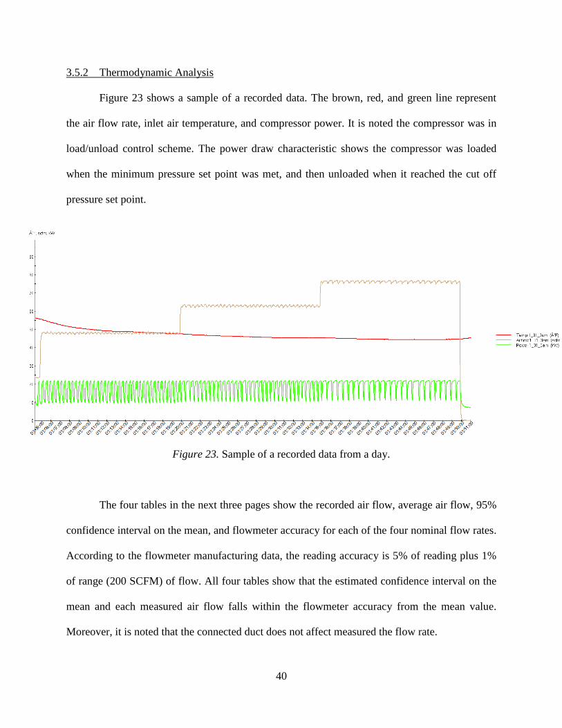
Figure 23 shows a sample of a recorded data. The brown, red, and green line represent

the air flow rate, inlet air temperature, and compressor power. It is noted the compressor was in

load/unload control scheme. The power draw characteristic shows the compressor was loaded

when the minimum pressure set point was met, and then unloaded when it reached the cut off

pressure set point.

Figure 23. Sample of a recorded data from a day.

The four tables in the next three pages show the recorded air flow, average air flow, 95%

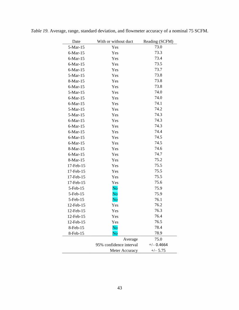
confidence interval on the mean, and flowmeter accuracy for each of the four nominal flow rates.

According to the flowmeter manufacturing data, the reading accuracy is 5% of reading plus 1%

of range (200 SCFM) of flow. All four tables show that the estimated confidence interval on the

mean and each measured air flow falls within the flowmeter accuracy from the mean value.

Moreover, it is noted that the connected duct does not affect measured the flow rate.

41

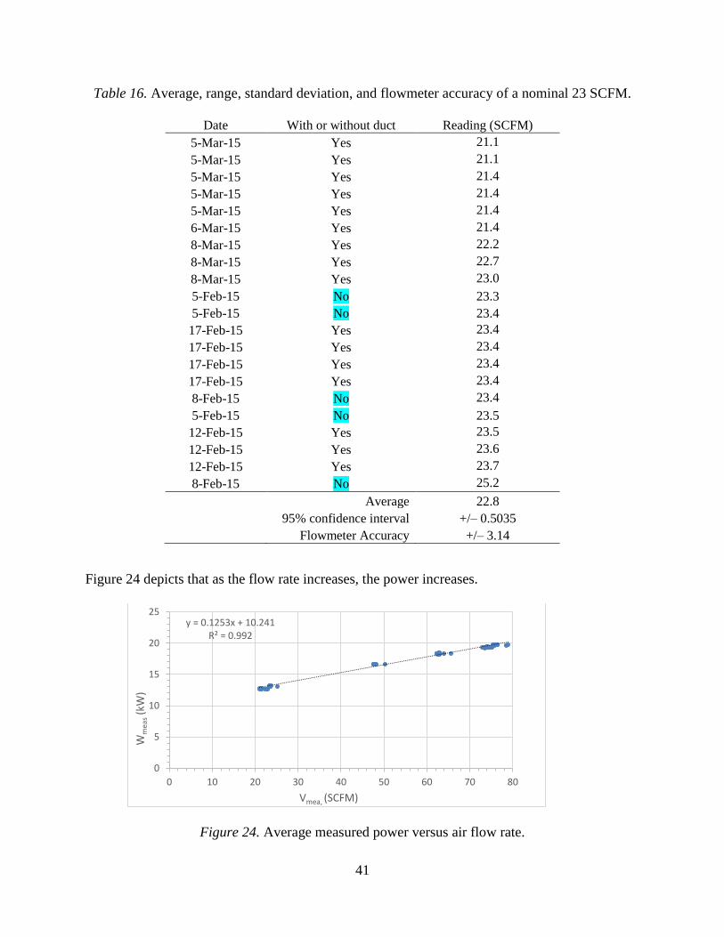
Table 16. Average, range, standard deviation, and flowmeter accuracy of a nominal 23 SCFM.

Date With or without duct Reading (SCFM)

5-Mar-15 Yes 21.1

5-Mar-15 Yes 21.1

5-Mar-15 Yes 21.4

5-Mar-15 Yes 21.4

5-Mar-15 Yes 21.4

6-Mar-15 Yes 21.4

8-Mar-15 Yes 22.2

8-Mar-15 Yes 22.7

8-Mar-15 Yes 23.0

5-Feb-15 No 23.3

5-Feb-15 No 23.4

17-Feb-15 Yes 23.4

17-Feb-15 Yes 23.4

17-Feb-15 Yes 23.4

17-Feb-15 Yes 23.4

8-Feb-15 No 23.4

5-Feb-15 No 23.5

12-Feb-15 Yes 23.5

12-Feb-15 Yes 23.6

12-Feb-15 Yes 23.7

8-Feb-15 No 25.2

Average 22.8

95% confidence interval +/– 0.5035

Flowmeter Accuracy +/– 3.14

Figure 24 depicts that as the flow rate increases, the power increases.

Figure 24. Average measured power versus air flow rate.

y = 0.1253x + 10.241R² = 0.992

0

5

10

15

20

25

0 10 20 30 40 50 60 70 80

Wm

eas

(kW

)

Vmea, (SCFM)

42

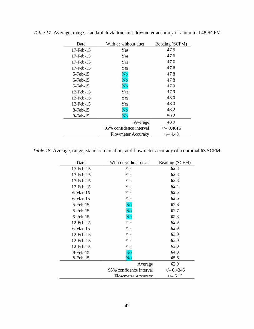
Table 17. Average, range, standard deviation, and flowmeter accuracy of a nominal 48 SCFM


17-Feb-15 Yes 47.5

17-Feb-15 Yes 47.6

17-Feb-15 Yes 47.6

17-Feb-15 Yes 47.6

5-Feb-15 No 47.8

5-Feb-15 No 47.8

5-Feb-15 No 47.9

12-Feb-15 Yes 47.9

12-Feb-15 Yes 48.0

12-Feb-15 Yes 48.0

8-Feb-15 No 48.2

8-Feb-15 No 50.2

Average 48.0





17-Feb-15 Yes 62.3

17-Feb-15 Yes 62.3

17-Feb-15 Yes 62.3

17-Feb-15 Yes 62.4

6-Mar-15 Yes 62.5

6-Mar-15 Yes 62.6

5-Feb-15 No 62.6

5-Feb-15 No 62.7

5-Feb-15 No 62.8

12-Feb-15 Yes 62.9

6-Mar-15 Yes 62.9

12-Feb-15 Yes 63.0

12-Feb-15 Yes 63.0

12-Feb-15 Yes 63.0

8-Feb-15 No 64.0

8-Feb-15 No 65.6

Average 62.9



43



5-Mar-15 Yes 73.0

6-Mar-15 Yes 73.3

6-Mar-15 Yes 73.4

6-Mar-15 Yes 73.5

6-Mar-15 Yes 73.7

5-Mar-15 Yes 73.8

8-Mar-15 Yes 73.8

6-Mar-15 Yes 73.8

5-Mar-15 Yes 74.0

6-Mar-15 Yes 74.0

6-Mar-15 Yes 74.1

5-Mar-15 Yes 74.2

5-Mar-15 Yes 74.3

6-Mar-15 Yes 74.3

6-Mar-15 Yes 74.3

6-Mar-15 Yes 74.4

6-Mar-15 Yes 74.5

6-Mar-15 Yes 74.5

8-Mar-15 Yes 74.6

6-Mar-15 Yes 74.7

8-Mar-15 Yes 75.2

17-Feb-15 Yes 75.5

17-Feb-15 Yes 75.5

17-Feb-15 Yes 75.5

17-Feb-15 Yes 75.6

5-Feb-15 No 75.9

5-Feb-15 No 75.9

5-Feb-15 No 76.1

12-Feb-15 Yes 76.2

12-Feb-15 Yes 76.3

12-Feb-15 Yes 76.4

12-Feb-15 Yes 76.5

8-Feb-15 No 78.4

8-Feb-15 No 78.9

Average 75.0


Meter Accuracy +/– 5.75

44

Figure 25 shows that the power does not vary with the inlet air temperature. Likewise,

Figure 26 shows the power does not vary with the inlet oil temperature. At each different

nominal flow rate, the power stays fairly constant with the varying inlet air temperature. All four

trend line equations show almost zero slope.

Figure 25. Power versus inlet air temperature at different nominal set flow rate.

Figure 26. Power versus inlet oil temperature at different nominal set flow rate.

y = -0.0026x + 13.104R² = 0.1556

y = -0.0003x + 16.651R² = 0.1392

y = -0.0009x + 18.393R² = 0.3052

y = -0.003x + 19.703R² = 0.3299

0

5

10

15

20

25

0 20 40 60 80 100 120

Wm

eas

(kW

)

Tair,in, (F)

23 SCFM 48 SCFM 63 SCFM 75 SCFM

y = -0.0095x + 14.127R² = 0.2905

y = -0.0006x + 16.713R² = 0.056

y = -0.0027x + 18.711R² = 0.3445

y = -0.0087x + 20.75R² = 0.275

0

5

10

15

20

25

100 110 120 130 140 150 160 170

Wm

eas

(kW

)

Inlet Oil Temperature (˚F)


45

The isentropic work can be calculated by using Equation 10. Equation 10 shows that the

inlet temperate is linearly dependent on the isentropic work. The specific measured work can be

calculated as shown in Equation 15. The inlet mass flow rate at the actual condition is

approximated by the mass flow rate at the standard condition since the moisture has only a fairly

small impact. This will eliminate some errors by not using estimation equations to determine the

inlet mass flow rate.

𝑤𝑚𝑒𝑎𝑠 =𝑊𝑚𝑒𝑎𝑠𝜂𝑚𝑜𝑡𝑜𝑟𝜂𝑡𝑟𝑎𝑛𝑠

𝜌std𝑉prod

Eq. 15

where,

ηmotor = motor efficiency, 92.4%, obtained from CAGI

ηtrans = transmission efficiency, estimated 93%

ρstd = air density at the standard condition,

𝑉𝑝𝑟𝑜𝑑 = measured volumetric flow rate and estimated blowdown rate (SCFM)

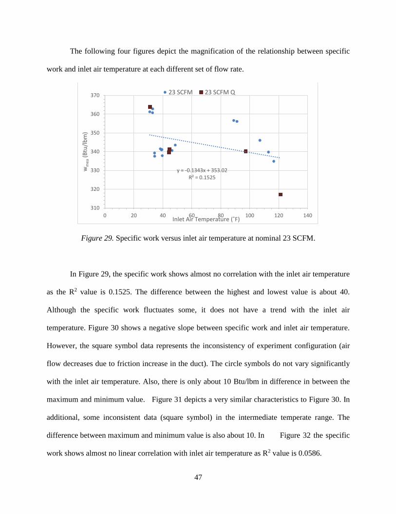
Figure 27 shows that inlet air temperature is not a factor in compressor specific work. In

fact, it shows the compressor specific work has an inverse relationship with airflow. More

specifically, the lower flow rate data scatter closely with a wide range of inlet air temperature.

Similarly, the intermediate and high flow rate data scatter closely at their corresponding specific

compressor power with a wide range of inlet air temperature.

Figure 28 indicates that the specific work does not vary significantly with inlet air

temperature. The square symbols, which has a “Q” in the legend, represent data collected

without the flexible duct connected to the inlet air suction. It is observed that the determined

specific work change at each different set of flow rate. This is mainly because of the compressor

control strategy efficiency. More specifically, in the load/unload control scheme, during

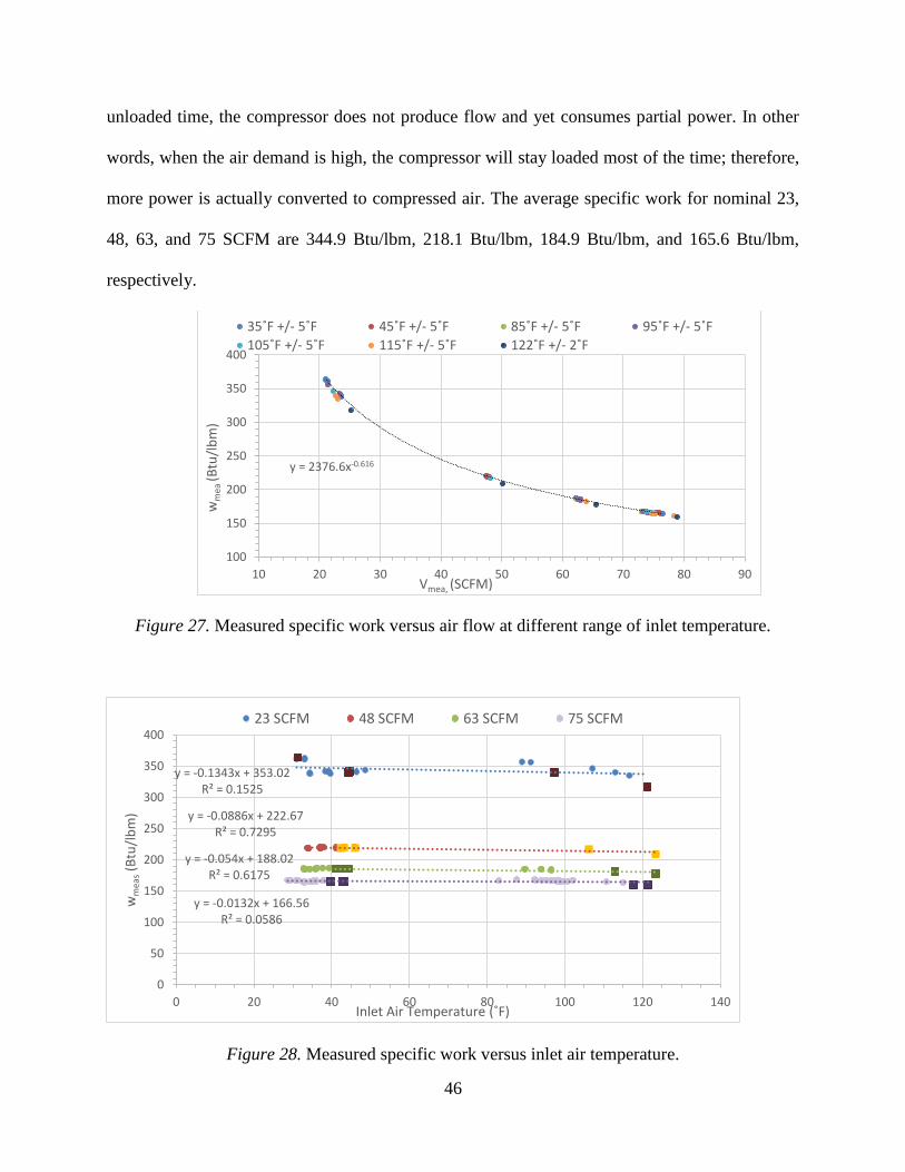
46

unloaded time, the compressor does not produce flow and yet consumes partial power. In other

words, when the air demand is high, the compressor will stay loaded most of the time; therefore,

more power is actually converted to compressed air. The average specific work for nominal 23,

48, 63, and 75 SCFM are 344.9 Btu/lbm, 218.1 Btu/lbm, 184.9 Btu/lbm, and 165.6 Btu/lbm,

respectively.

Figure 27. Measured specific work versus air flow at different range of inlet temperature.

Figure 28. Measured specific work versus inlet air temperature.

y = 2376.6x-0.616

100

150

200

250

300

350

400

10 20 30 40 50 60 70 80 90

wm

ea (B

tu/l

bm

)

Vmea, (SCFM)

35˚F +/- 5˚F 45˚F +/- 5˚F 85˚F +/- 5˚F 95˚F +/- 5˚F

105˚F +/- 5˚F 115˚F +/- 5˚F 122˚F +/- 2˚F

y = -0.1343x + 353.02R² = 0.1525

y = -0.0886x + 222.67R² = 0.7295

y = -0.054x + 188.02R² = 0.6175

y = -0.0132x + 166.56R² = 0.0586

0

50

100

150

200

250

300

350

400

0 20 40 60 80 100 120 140

wm

eas

(Btu

/lb

m)

Inlet Air Temperature (˚F)


47

The following four figures depict the magnification of the relationship between specific

work and inlet air temperature at each different set of flow rate.

Figure 29. Specific work versus inlet air temperature at nominal 23 SCFM.

In Figure 29, the specific work shows almost no correlation with the inlet air temperature

as the R2 value is 0.1525. The difference between the highest and lowest value is about 40.

Although the specific work fluctuates some, it does not have a trend with the inlet air

temperature. Figure 30 shows a negative slope between specific work and inlet air temperature.

However, the square symbol data represents the inconsistency of experiment configuration (air

flow decreases due to friction increase in the duct). The circle symbols do not vary significantly

with the inlet air temperature. Also, there is only about 10 Btu/lbm in difference in between the

maximum and minimum value. Figure 31 depicts a very similar characteristics to Figure 30. In

additional, some inconsistent data (square symbol) in the intermediate temperate range. The

difference between maximum and minimum value is also about 10. In Figure 32 the specific

work shows almost no linear correlation with inlet air temperature as R2 value is 0.0586.

y = -0.1343x + 353.02R² = 0.1525

310

320

330

340

350

360

370

0 20 40 60 80 100 120 140

wm

ea(B

tu/l

bm

)


23 SCFM 23 SCFM Q

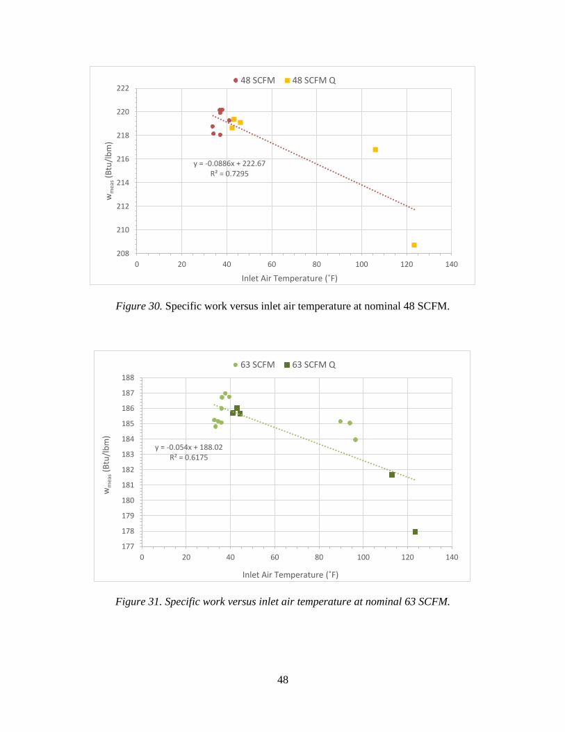
48



y = -0.0886x + 222.67R² = 0.7295

208

210

212

214

216

218

220

222

0 20 40 60 80 100 120 140

wm

eas

(Btu

/lb

m)


48 SCFM 48 SCFM Q

y = -0.054x + 188.02R² = 0.6175

177

178

179

180

181

182

183

184

185

186

187

188

0 20 40 60 80 100 120 140

wm

eas

(Btu

/lb

m)


63 SCFM 63 SCFM Q

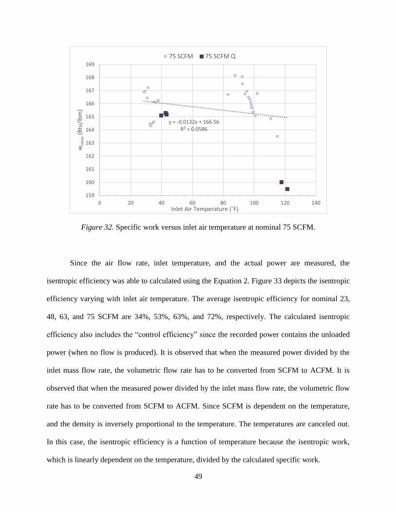
49


Since the air flow rate, inlet temperature, and the actual power are measured, the

isentropic efficiency was able to calculated using the Equation 2. Figure 33 depicts the isentropic

efficiency varying with inlet air temperature. The average isentropic efficiency for nominal 23,

48, 63, and 75 SCFM are 34%, 53%, 63%, and 72%, respectively. The calculated isentropic

efficiency also includes the “control efficiency” since the recorded power contains the unloaded

power (when no flow is produced). It is observed that when the measured power divided by the

inlet mass flow rate, the volumetric flow rate has to be converted from SCFM to ACFM. It is

observed that when the measured power divided by the inlet mass flow rate, the volumetric flow

rate has to be converted from SCFM to ACFM. Since SCFM is dependent on the temperature,

and the density is inversely proportional to the temperature. The temperatures are canceled out.

In this case, the isentropic efficiency is a function of temperature because the isentropic work,

which is linearly dependent on the temperature, divided by the calculated specific work.

y = -0.0132x + 166.56R² = 0.0586

159

160

161

162

163

164

165

166

167

168

169

0 20 40 60 80 100 120 140

wm

eas

(Btu

/lb

m)


75 SCFM 75 SCFM Q

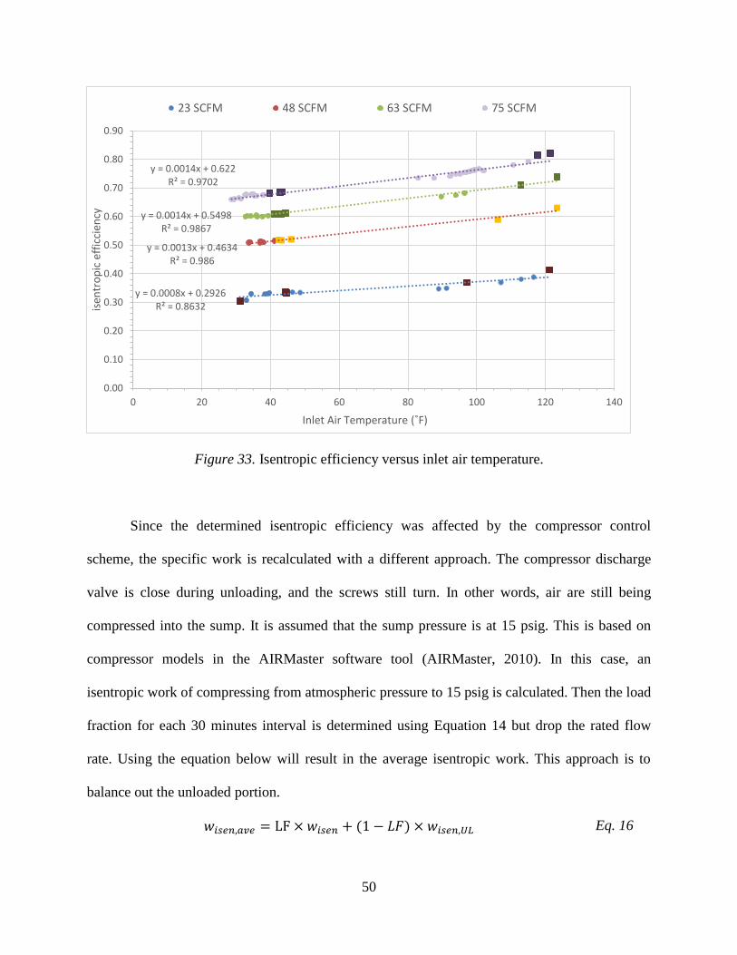
50

Figure 33. Isentropic efficiency versus inlet air temperature.

Since the determined isentropic efficiency was affected by the compressor control

scheme, the specific work is recalculated with a different approach. The compressor discharge

valve is close during unloading, and the screws still turn. In other words, air are still being

compressed into the sump. It is assumed that the sump pressure is at 15 psig. This is based on

compressor models in the AIRMaster software tool (AIRMaster, 2010). In this case, an

isentropic work of compressing from atmospheric pressure to 15 psig is calculated. Then the load

fraction for each 30 minutes interval is determined using Equation 14 but drop the rated flow

rate. Using the equation below will result in the average isentropic work. This approach is to

balance out the unloaded portion.

𝑤𝑖𝑠𝑒𝑛,𝑎𝑣𝑒 = LF × 𝑤𝑖𝑠𝑒𝑛 + (1 − 𝐿𝐹) × 𝑤𝑖𝑠𝑒𝑛,𝑈𝐿 Eq. 16

y = 0.0008x + 0.2926R² = 0.8632

y = 0.0013x + 0.4634R² = 0.986

y = 0.0014x + 0.5498R² = 0.9867

y = 0.0014x + 0.622R² = 0.9702

0.00

0.10

0.20

0.30

0.40

0.50

0.60

0.70

0.80

0.90

0 20 40 60 80 100 120 140

isen

tro

pic

eff

icci

ency



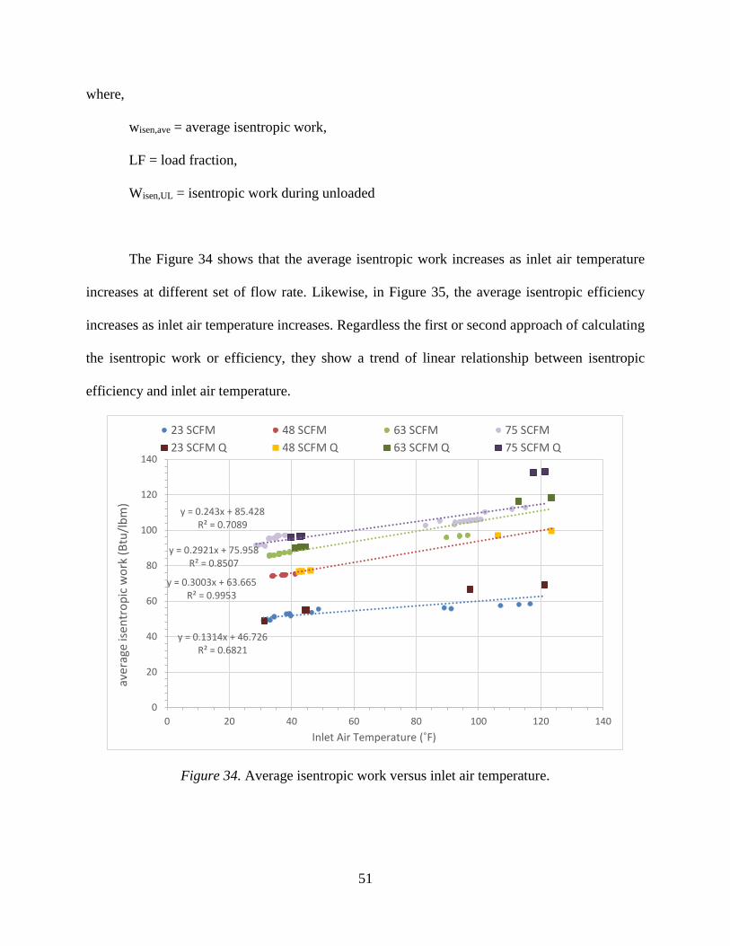
51

where,

wisen,ave = average isentropic work,

LF = load fraction,

Wisen,UL = isentropic work during unloaded

The Figure 34 shows that the average isentropic work increases as inlet air temperature

increases at different set of flow rate. Likewise, in Figure 35, the average isentropic efficiency

increases as inlet air temperature increases. Regardless the first or second approach of calculating

the isentropic work or efficiency, they show a trend of linear relationship between isentropic

efficiency and inlet air temperature.

Figure 34. Average isentropic work versus inlet air temperature.

y = 0.1314x + 46.726R² = 0.6821

y = 0.3003x + 63.665R² = 0.9953

y = 0.2921x + 75.958R² = 0.8507

y = 0.243x + 85.428R² = 0.7089

0

20

40

60

80

100

120

140

0 20 40 60 80 100 120 140

aver

age

isen

tro

pic

wo

rk (

Btu

/lb

m)



23 SCFM Q 48 SCFM Q 63 SCFM Q 75 SCFM Q

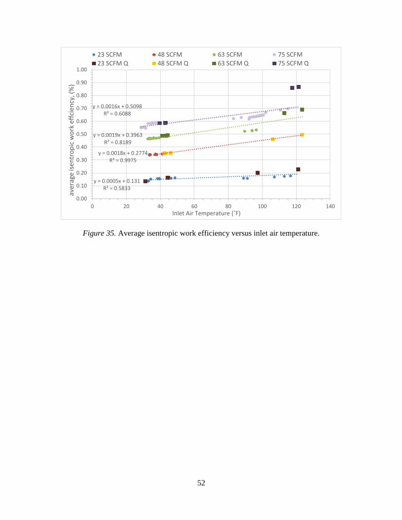
52

Figure 35. Average isentropic work efficiency versus inlet air temperature.

y = 0.0005x + 0.131R² = 0.5833

y = 0.0018x + 0.2774R² = 0.9975

y = 0.0019x + 0.3963R² = 0.8189

y = 0.0016x + 0.5098R² = 0.6088

0.00

0.10

0.20

0.30

0.40

0.50

0.60

0.70

0.80

0.90

1.00

0 20 40 60 80 100 120 140

aver

age

isen

tro

pic

wo

rk e

ffci

ency

, (%

)



23 SCFM Q 48 SCFM Q 63 SCFM Q 75 SCFM Q

53

CHAPTER 4: CONCLUSIONS

4.1 Summary

The first objective of this thesis is to determine the significant effects of air volumetric

flow rate, inlet air temperature, and oil inlet air temperature on the compressor power via the

design of experiment technique. More specifically, three models are developed to investigate this

objective. These models are 3F2L–CP, 2F2L–CP, and 2F2L–IOT. In the 3F2L–CP model, the

result shows that only air volumetric flow rate contributes to the compressor power consumption.

This result is fairly accurate, although the orthogonality property is not as close to the desired

state. In the 2F2L–CP, the result shows that volumetric flow rate variable contributes far more

than inlet air temperature on the compressor power consumption. In the 2F2L–IOT, inlet air

temperature contributes slightly more than the air flow rate to the inlet oil temperature. In these

two models, the designed matrixes meet the orthogonality property.

The second objective is to investigate the correlation between inlet air temperature and

the compressor power consumption through thermodynamic analysis. It is observed that

compressor power consumption is linearly dependent on the volumetric flow rate. Also, the data

shows that compressor power consumption does not vary with the inlet air and oil temperature.

Furthermore, the measured specific work varies fairly constantly with the inlet air temperature.

Two approaches are performed to determine the isentropic efficiency. Both results suggest that

the isentropic efficiency increases as the inlet air temperature increases. The determined

isentropic efficiency ranges between 30% and 80% for the first method, and varies between 10%

54

and 90% for the second method. A wide range of isentropic efficiency is determined mainly

because of the load/unload control scheme. The compressor will still draw a portion of power

(unloaded power) although it does not produce any compressed air. This unloaded power is

included in the analysis.

In conclusion, many professionals or reliable sources advocate the use of lower intake air

temperature for air compressor to lower the power consumption; however, these experimental

results reflect that the inlet air and oil temperature have little or no contribution to an oil-

lubricated rotary screw air compressor. In fact, results show that the overall compressor power is

highly dependent on the air volumetric flow rate and the control scheme.

4.2 Future Work

This thesis explores only the effect of inlet air temperature on an oil-lubricated rotary screw

compressor. For future work, more data can be collected at the intermediate and high

temperature range to support this thesis. Also, the oil mass flow rate can be measured and

accounted for in the compressor power thermodynamic equation. This is because the power draw

also compresses the injected-oil. Moreover, a similar experiment can be performed on another

compressor’s control types, such as inlet–modulation, since the load/unload control scheme

significantly affects the compressor efficiency. Furthermore, another experiment can be

conducted to investigate the effect of inlet air temperature on an oil-free rotary screw

compressor.

55

REFERENCES

AIRMaster. (2010). [computer software]. http://energy.gov/eere/amo/articles/airmaster

Batchelor, M. (1998). Benefits of Remotely Monitoring Rotary Screw Air Compressors. Plant

Engineering, 52, 77-80.

Bloch, H. P. (2006). A Practical Guide to Compressor Technology. New Jesey: John Wiley &

Sons, Inc.

CAGI Compressed Air & Gas Institute. (2012). Conversion of SCFM to ACFM. Working With

Compressed Air. Retrieved March 20, 2015, from

http://www.cagi.org/working-with-compressed-air/conversion-scfm-

acfm.aspx#!prettyPhoto

Cengel, Y. A., & Boles, M. A. (2011). Thermodynamics: An Engineering Approach. New York:

McGraw-Hill.

Chukanova, E., Stosic, N., Kovacevic, A., & Dhunput A. (2012). Investigation of Start Up

Process in Oil Flooded Twin Screw Compressors. International Compressor Engineering

Conference, Paper 2048.

Hicks, T. G. (2006). Economics of Air Compressor Inlet Location. Handbook of Mechanical

Engineering Calculations, 2nd ed. Retrieved January 18, 2015 from Access Engineering

database.

Kakaras, E., Doukelis, A., & Karellas, S. (2004). Compressor intake-air cooling in gas turbine

plants. Efficiency, Costs, Optimization, Simulation and Environmental Impact of Energy

Systems, 29, 12-15. Retrieved from

http://www.sciencedirect.com/science/article/pii/S0360544204001227

Kaya, D., Phelan, P., Chau, D., & Sarac, H. I. (2002). Energy Conservation in Compressed-Air

Systems. International Journal of Energy Research, 26(9), 837-849.

Ravi Kumar, N., Rama Krishna, K., & Sita Rama Raju, A. V. (2007). Performance Improvement

and Exergy Analysis of Gas Turbine Powe Plant with Alternative Regenerator and Intake

Air Cooling. Energy Engineering, 104:3, 36-53

Martinez, L. C, Guillen, D., Prada, J., Conteras A. (2012). Thermoeconomic Model for the

Energy optimization of Industrial Air Compressed Supply Network under Transient

http://www.cagi.org/working-with-compressed-air/conversion-scfm-acfm.aspx#!prettyPhoto

http://www.cagi.org/working-with-compressed-air/conversion-scfm-acfm.aspx#!prettyPhoto

56

Condition. ASME 2012 International Mechanical Engineering Congress & Exposition, 6,

1589-1593.

National Weather Service Weather Forecast Office (2014). Vapor Pressure. Retrieved March 20,

2015, from

http://www.srh.noaa.gov/images/epz/wxcalc/vaporPressure.pdf

NIST/SEMATECH (2013). E-Handbook of Statistical Method. Retrieved March 20, 2015, from

http://www.itl.nist.gov/div898/handbook/pri/section3/pri3331.htm

Office of Energy Efficiency & Renewable Energy & Compressed Air Challenge. (2003)

Improving Compressed Air System Performance: A Sourcebook for Industry. Retrieved

February 20, 2015 from

https://www1.eere.energy.gov/manufacturing/tech_assistance/pdfs/compressed_air_sourc

ebook.pdf

Parekh, P. S. (2000). Investment-Grade Compressed Air System Audit, Analaysis, and Upgrade

in a Pulp & Papper Mill. 22nd Annual Industrial Energy Technology Conference in

Houston. Texas, USA.

U.S Department of Energy. (2004). Effect of Intake on Compressor Performance. Compressed

Air Tip Sheet #14. Retrieved February 20, 2015 from

http://www.compressedairchallenge.org/library/tipsheets/tipsheet14.pdf

U.S Department of Energy. (2004). Determine the Cost of Compressed Air for Your Plant.

Compressed Air Tip Sheet #1. Retrieved from April 12, 2015.

https://www.compressedairchallenge.org/library/tipsheets/tipsheet01.pdf

U.S Department of Energy. (2003). Heat Recovery with Compressed Air Systems. Compressed

Air Systems Fact Sheet #10. Retrieved March 26, 2015 from

https://www.compressedairchallenge.org/library/factsheets/factsheet10.pdf

Stosic, N. (2015). On Heat Transfer in Screw Compressors. International Journal of Heat and

Fluid Flow, 51, 285-297.

http://www.itl.nist.gov/div898/handbook/pri/section3/pri3331.htm

https://www1.eere.energy.gov/manufacturing/tech_assistance/pdfs/compressed_air_sourcebook.pdf

https://www1.eere.energy.gov/manufacturing/tech_assistance/pdfs/compressed_air_sourcebook.pdf

https://www.compressedairchallenge.org/library/factsheets/factsheet10.pdf