

EXPERIMENTS ON THE STABILITY OF SHEATHED COLD-FORMED STEEL
STUDS UNDER AXIAL LOAD AND BENDING
by Kara D. Peterman
A thesis submitted in Johns Hopkins University in conformity with the requirements for
the degree of Master of Science in Engineering.
Baltimore, Maryland March 2012

ii
Abstract
This report provides test and analysis results for a typical cold-formed steel (CFS) stud as
employed in light steel framing for a building. Specifically, tests are conducted on a
362S162-68 (50 ksi) stud connected to 362T162-68 (50ksi) track with varying
combinations of sheathing connected to the two flanges. Loading consists of both axial
load and a directly applied horizontal load to induce major-axis bending of the stud (and
torsion due to the shear center of the stud). The sheathing configurations studied are
intended to capture various stages of construction and final form and include: no
sheathing; one-sided sheathing with Oriented Strand Board (OSB); and two-sided
sheathing with OSB and gypsum board, or only OSB on the two sides, or only gypsum
board on the two sides. The combinations of axial load (P) and bending load (M) studied
are intended to capture nearly the complete P-M space.
The work is an extension of earlier tests on axially loaded sheathed studs under a similar
configuration (Vieira 2011). Vieira’s (2011) work demonstrated that: (a) tests on
sheathed single studs provided the same response as tests on full walls with 5 studs; (b)
sheathing is remarkably effective in stabilizing CFS studs and for cases with sheathing on
both faces both global and distortional buckling are restricted and only local buckling
remains; (c) end boundary conditions are highly influential in the results and are found to
be closest to fixed ends for restricting global modes. Utilizing (a) the beam-column tests
conducted here are only on single stud specimens. Similar to (b) the beam-column tests
here show the significant strength increases to be had due to the introduction of sheathing

iii
to stabilize the stud. However, contrary to (c) it is found that under major-axis bending
the sheathed stud behaves as having pinned end boundary conditions. In addition, the
beam-column tests show the importance of the addition of direct torsion into the behavior
(due to the shear center of the stud). One-sided sheathing cases cannot meaningfully
restrict the torsion, and for two-sided sheathing cases it must still be considered at least in
terms of the fastener limit states. The analysis of Vieira (2011) is extended to beam-
columns for the member limit states and a new method is developed for the fastener limit
states – combined the results are shown to be in reasonable agreement with the testing,
but room for improvement remains. Specifically fastener demands developed from the
torsion in bending are more involved than is typically recognized in current design
(stiffness analysis is needed to properly determine the demands) and leads to some
unwanted complication in design. Taken in total the test and analysis results provided
herein demonstrate how sheathing improves the behavior of CFS stud walls and provides
the details necessary to develop a comprehensive design method, including for dis-
similarly sheathed studs.
Advisor: Benjamin Schafer, Professor and Chair
Department of Civil Engineering, Johns Hopkins University

iv
“New worlds to conquer!”
For Team Peterman

v
Acknowledgments
My family often jokes, in reference to the novel, The Seven Pillars of Wisdom, by T.E.
Lawrence, that academic degrees are pillars of wisdom. This is not in reference to their
scholarly nature, but rather, to the shape diplomas hold when traditionally rolled, secured
with a ribbon, and stood on their ends. The family record currently stands at six pillars,
and I am thrilled to narrow the gap, if only slightly.
The conquest of my second pillar of wisdom was far from lonely. I am thankful to have
incredible friends, both near and far, who invigorate me with their passions. My adviser,
Ben Schafer, has been a great motivator—his energy and enthusiasm are not only
contagious, but also more effective than the strongest espresso. My mom and dad have
unconditionally supported me not only in my great passions, but also in the multitude of
other things I am continually sticking my nose in. For this, I am forever thankful.
For many, the completion of a thesis is an ending. In my case, it is the end of my Masters
work but the symbolic beginning of my PhD work. Therefore, it is appropriate to yet
again draw from Lawrence: “So they allowed it to begin…”
This thesis was prepared as part of the American Iron and Steel Institute sponsored project: Sheathing Braced Design of Wall Studs. The project also received supplementary support and funding from the Steel Stud Manufacturers Association. Project updates are available at www.ce.jhu.edu/bschafer/sheathedwalls. Any opinions, findings, and conclusions or recommendations expressed in this publication are those of the author(s) and do not necessarily reflect the views of the American Iron and Steel Institute, nor the Steel Stud Manufacturers Association.

vi
TABLE OF CONTENTS
Abstract ii Acknowledgments v Chapter 1 – Introduction 1 Chapter 2 - Test Setup 3
2.1 - Testing Rig 3 2.2 - Specimen Design 4 2.3 - End Conditions 7 2.4 - Sensor Plan 9 2.5 - Load Protocol 12 2.6 - Load Location 15
Chapter 3 - Test Matrix 17 Chapter 4 - Material Properties 18 Chapter 5 - Section 24 Chapter 6 - Imperfections 26 Chapter 7 – Results 30
7.1 – OO Specimens 39 7.2 – GG Specimens 40 7.3 – GO Specimens 41 7.4 – OB Specimens 43 7.5 – BO Specimens 44 7.6 – BB Specimens 46 7.7 – OG Specimens 47
Chapter 8 – Nominal Capacity Analysis 48 8.1 Local Buckling Member Capacity 48 8.2 Sheathing Braced Member Capacity 50 8.3 Fastener/Connection limit state capacities 53
Chapter 9 – Discussion 57 9.1 - Load Location 57 9.2 - End Conditions 58 9.3 – Comparison of member limit states to tested capacity 62 9.4 – Role of fastener stiffness in determining fastener demand 65 9.5 – Demands and Fastener Limit States 69
Chapter 10 – Future Work 76 Chapter 11 – Conclusions 77 Appendices 81
Appendix A: Specimen reference (Shifferaw, et al., 2010) 81 Appendix B: Tensile Results 82 Appendix C: Tensile Specimen Measurements 84 Appendix D: Complete Imperfection Measurements 85 Appendix E: Complete Cross-Section Measurements 86 Appendix F: Temperature and Humidity Readings in JHU Laboratory 88 Appendix G: Addendum Test with 2 in. fastener spacing 89 Appendix H: Complete Specimen Response Summaries 90

1
Chapter 1 – Introduction
Cold-formed steel (CFS) is emerging in the light-framed construction field as an efficient,
light, and economic material for both structural and non-structural elements. CFS
members are commonly sheathed in oriented stand board or gypsum to frame walls and
other architectural elements. This sheathing is not entirely without structural purpose: it
can brace the CFS stud under load via the fastener connection.
Cold-formed steel members as beams and columns have been thoroughly investigated,
and their behavior implemented in the American Iron and Steel Institute (AISI)
Specification. Recent research by Vieira (2011) worked towards extending this
investigation to sheathed cold-formed steel columns under axial load. Vieira also
characterized the behavior of the sheathing-fastener-stud system by dividing the system
stiffness into local fastener and global diaphragm stiffness. The research presented herein
expands the cold-formed steel literature to include the behavior of sheathed CFS columns
under axial load and bending.
Winter (1947) was the first to recognize the change in behavior and increase in capacity
of CFS studs due to the stud-sheathing connection. This body of work ultimately
concluded that connection stiffness was the major contributor to the stud limit state,
although only considering flexural buckling and requiring numerous assumptions.
Despite the limitations in this method, it was adopted by AISI in 1962. Simaan and Peköz
developed the diaphragm stiffness method as an alternative to Winter’s method in 1976,
considering flexural, torsion, and flexural-torsional modes. The diaphragm method was
2
adopted, but ultimately dropped from the Specification in favor of Winter’s earlier
method.
Other researchers have studied cold-formed steel stud assemblies. Significantly, Okasha
(2004) and Fiorino (2007?) examined fastener stiffness under axial and cyclic loading in
stud-to-sheathing connections. Telue (2001) characterized the behavior of steel stud
framing lined in plasterboard and Miller (1994) accomplished the same for gypsum. As
briefly mentioned previously, Vieira (2011) employed experimental and analytical
methods to develop a design method that considers translational and rotational local
stiffnesses, as well as the diaphragm stiffness of the sheathing. A new design approach is
proposed for implementation in the AISI Specification for determing elastic buckling
loads for CFS members with sheathing.

3
Chapter 2 - Test Setup
2.1 - Testing Rig
The Johns Hopkins University multi-degree of freedom (MDOF) testing rig was used for
this series of tests. The MDOF rig can load full-scale walls and columns with axial load,
shear, and bending, although only axial load and bending were employed in this test
series. Figure 1 depicts the MDOF rig with a single column specimen.
(a). Isotropic view of MDOF testing rig (b). Side view of MDOF testing rig
Figure 1: Johns Hopkins University MDOF testing rig
The specimen is connected to the loading beam on top and the ‘ground’ beam on bottom.
Four hydraulic actuators apply axial load while one actuator applies bending moment in
the form of a horizontal load at specimen mid-height.
4
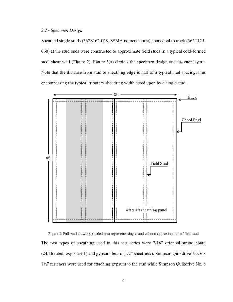
2.2 - Specimen Design
Sheathed single studs (362S162-068, SSMA nomenclature) connected to track (362T125-
068) at the stud ends were constructed to approximate field studs in a typical cold-formed
steel shear wall (Figure 2). Figure 3(a) depicts the specimen design and fastener layout.
Note that the distance from stud to sheathing edge is half of a typical stud spacing, thus
encompassing the typical tributary sheathing width acted upon by a single stud.
Figure 2: Full wall drawing, shaded area represents single stud column approximation of field stud
The two types of sheathing used in this test series were 7/16” oriented strand board
(24/16 rated, exposure 1) and gypsum board (1/2” sheetrock). Simpson Quikdrive No. 6 x
1!” fasteners were used for attaching gypsum to the stud while Simpson Quikdrive No. 8
Chord Stud
Field Stud
Track
4ft x 8ft sheathing panel
8ft
8ft

5
x 1 15/16” were used for the oriented strand board (OSB). The boards were stored in the
JHU laboratory with an average humidity of 56% and temperature of 22°C (71°F) over
102 days. A full record of the lab environmental conditions leading up to testing is
provided in Appendix F: Temperature and Humidity Readings in JHU Laboratory.
(a). Fastener layout and specimen design (b). Sensor plan (numbers in blue)
Figure 3: Single column specimen design (in.)
Specimens were named based on the stud number and sheathing orientation. For example,
S05-OG corresponds to stud number 05, sheathed with OSB (O) on the non-loaded face
and gypsum (G) on the loaded face. Figure 4 provides a detailed example.

6
Figure 4: Nomenclature example
Seven different sheathing combinations were tested. These are summarized in Table 1. It should be noted that in the specimens left bare on the loading face, the load
was applied directly to the stud.
Table 1: Summary of tested sheathing configurations
Type Non-Load Face Load Face BB B, Bare B, Bare BO B, Bare O, OSB OB O, OSB B, Bare GG G, Gypsum G, Gypsum GO G, Gypsum O, OSB OG O, OSB G, Gypsum OO O, OSB O, OSB
LOAD FACE Gypsum, G
Non-Loaded OSB, O
Horizontal Load
AX
IAL
AX
IAL
S 05 - O G stud number
and test index
WEST SIDE: Sheathing type on non-loaded
face.
EAST SIDE: Sheathing type on loaded face.

7
2.3 - End Conditions
Special consideration of the column end conditions was required to best approximate a
continuous full wall. In a full wall, the track connected to field studs is restricted from
twist by virtue of being connected to adjacent studs. To simulate this behavior, track ends
were clamped to the base and load beam of the MDOF testing rig via steel plates that
blocked the track from movement. This clamping system used to fix the track ends to the
machine is drawn in Figure 5.
Figure 5: Drawing of end conditions (in.)
The clamping system (Figure 5) consists of four main components: a "” plate used for
blocking the end of the track; the threaded rod and bolt responsible for applying the
clamping force; a 6” steel plate used for mounting the track ends to the testing rig and; a

8
short piece of track used as a spacer plate in between the blocking plate and testing rig
mount. These components are identified in the photograph in Figure 6.
Figure 6: Key components of clamping system
The column tracks were also connected to the testing rig via a "” bolt that goes through a
machined hole in the track into a mounting plate connected to the MDOF rig. This bolt
hole is located at the center of the track and corresponds to the approximate centroid of
the stud.
(a). Top view of rig-to-track connection (b). Side view of rig-to-track connection
Figure 7: Detail of connection from middle of track to testing rig
Column end conditions are summarized in Figure 8.
Short piece of track used as a spacer
Column sheathing Track end
Testing rig base
Steel plate track- to-rig mount
!” clamping plate

9
Figure 8: Photographic summary of column end conditions
2.4 - Sensor Plan
Thirteen sensors were employed to measure the response of the specimen under load.
Eleven position transducers were connected to the specimen itself and two string
potentiometers were connected to the testing rig alone to accurately capture machine
displacement. Figure 9 depicts the sensor layout and numbering scheme. Position
transducers 5 and 6 capture twist in the sheathing and in combination with 7 and 11,
record column displacement in the direction of the horizontal load application. To record
motion of the stud during loading, sensors were arranged as triplets (9, 10, 8 and 4, 3, 2)
and captured relative twist of the stud and local buckling waves in the middle of the stud
web.
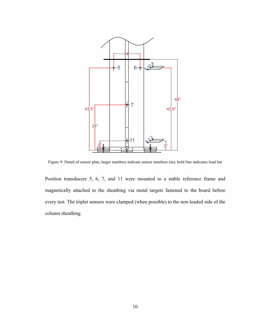
10
Figure 9: Detail of sensor plan; larger numbers indicate sensor numbers (in); bold line indicates load bar
Position transducers 5, 6, 7, and 11 were mounted to a stable reference frame and
magnetically attached to the sheathing via metal targets fastened to the board before
every test. The triplet sensors were clamped (when possible) to the non-loaded side of the
column sheathing.

11
(a). Isometric view (b). Side view
Figure 10: Photograph of position transducers 5, 6, 7, and 11
Figure 11: Triplet sensors 9, 8, and 10, located at loading height

12
A drawback to this sensor configuration was that the mid-height sensor triplet, containing
sensors 8, 9, and 10, had to be removed during testing, otherwise the horizontal loading
bar would compress the sheathing onto the sensors and the sheathing would gain stiffness
unrealistically. Unfortunately, this point occurred before the specimen had attained its
peak load.
2.5 - Load Protocol
Figure 12 demonstrates an idealization of the specimen under both axial load (P) and
horizontal load (H). The quantities in Figure 12 are relatively easy to discern, with the
exception of torsion, due to the inherent difficulty in obtaining the eccentricity (e) of the
load application point to the shear center of the cross-section (refer to Figure 14). This
will be discussed further in Section 1.6.
Figure 12: Loading and response idealization
Loading Idealization Axial Load Moment (drawn on tension side)
Shear Force Torsion
H, !
P, "
HL4
H2
H2
He2
He2
He
L

13
Two load protocols were employed in this series of testing. The first, used for a majority
of the specimens, was in displacement control and involved loading the stud with a pre-
determined percentage of its axial capacity determined from previous stud tests
(Shifferaw, et al. 2010) and then holding the axial displacement at this level, and then
loading the stud at mid-height with a horizontal displacement until failure. The axial load
was allowed to degrade as the horizontal load increased (and caused axial load relieving
end shortening). The dashed line in Figure 13 represents this protocol.
In the second protocol, the load control protocol, axial load is maintained as horizontal
displacement increases. Once the stud has attained the pre-determined percentage of axial
load, horizontal displacement and additional axial displacement are applied together such
that axial load remains approximately constant. Only two specimens were loaded in this
manner to achieve a true 80% of Pmax at failure, rather than the lower percentage
(achieved in S30-GG). Figure 13 compares the two protocols for specimens S39-GG and
S30-GG.

14
Figure 13: Plot of P-M space for two GG specimens with differing load protocols
In the case of the constant axial displacement protocol, axial displacement was applied at
an average of 0.2 in. over 5 minutes, or 0.0469 in./min. It should be noted that this
loading rate was not enforced with particular diligence, and varies slightly from specimen
to specimen, based on machine location and desired axial load. However, in specimens
taken to larger axial load values, loading rate was decreased so as to not fail the
specimens (via rapid load rate) before their pre-determined peak axial capacity.
That rate at which horizontal load was applied was stringently enforced at 1.5” over 32
minutes, or 0.0469”/min. The specimen was loaded until past peak.
0 0.05 0.1 0.15 0.2 0.25 0.3 0.35 0.4 0.45 0.5
0
0.1
0.2
0.3
0.4
0.5
0.6
0.7
0.8
M/Mynom
P/P yn
om
S39 GG
S30 GG
constant axial loadconstant axial displacement

15
In the constant axial load protocol, axial displacement rate was the same as in the
constant axial displacement protocol up until horizontal load was applied. At that point,
an estimate was made as to how much additional displacement was required to maintain
axial load, and that displacement was applied at the same rate as the horizontal load.
2.6 - Load Location
While the location of the horizontal load H along the length of the specimen has been
discussed, the point at which the load is applied to the cross-section must not be
neglected. This location ultimately induces torsion in the member as a result of the
eccentricity to the shear center. This is represented in Figure 14.
Figure 14: Load location on cross-section
However, this location is not static and may dramatically change throughout the duration
of a test. As illustrated in Figure 14, the test begins with the load bar pushing against the
flat portion of the stud flange. Increasing horizontal load causes torsion in the specimen
H (resultant)
e
shear center
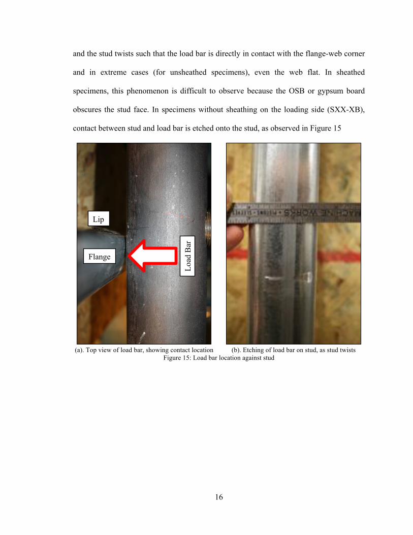
16
and the stud twists such that the load bar is directly in contact with the flange-web corner
and in extreme cases (for unsheathed specimens), even the web flat. In sheathed
specimens, this phenomenon is difficult to observe because the OSB or gypsum board
obscures the stud face. In specimens without sheathing on the loading side (SXX-XB),
contact between stud and load bar is etched onto the stud, as observed in Figure 15
(a). Top view of load bar, showing contact location (b). Etching of load bar on stud, as stud twists
Figure 15: Load bar location against stud
Load
Bar
Flange
Lip

17
Chapter 3 - Test Matrix
A test matrix (Table 2) was constructed in an attempt to define the interaction space
(axial load versus bending—the P-M space) for studs sheathed with combinations of OSB,
gypsum, and no sheathing at all.
Table 2: Test Matrix
Loading Sheathing (B=Bare, G=Gypsum, O=OSB) P H BB OB GG OG OO
100% 0
5 (2') 18 (2') 19 (2') 20 (2') 21 (2') 6 (4') 14 (4') 15 (4') 16 (4') 17 (4') 7 (6') 12 (6') 10 (6') 13 (6') 9 (6') 22 (8') 23 (8') 25 (8') 24 (8') 26 (8')
P H BB OB BO GG OG GO OO ~80%P to failure xx xx xx S39 xx xx S18 #80%P to failure xx S21 S37 S23,S30 S32 S16 S15 # 60%P to failure S34 S14 S27 S20 S36 S08 S38 # 40%P to failure S26 S10 S13 S19 S05 S09 S01 # 10%P to failure xx S06 xx S12 S07 S33 S11
Legend:
Refers to existing test results of Vieira and Schafer, Vieira et al. first number is index, second number is length xx This configuration not tested S# This test series (Peterman and Schafer)
B=Bare, no sheathing
G=1/2 in. gypsum board fastened with #6 Simpson Strong Tie fasteners at 12 in. o.c.
O=7/16 in. OSB board fastened with #8 Simpson Strong Tie fasteners at 12 in. o.c. OB = OSB on west side, Bare on East Side (load applied) --> BO = Bare on west side, OSB on East Side (load applied)
The shaded area refers to a series of tests performed in Vieira et al. (2010).
18
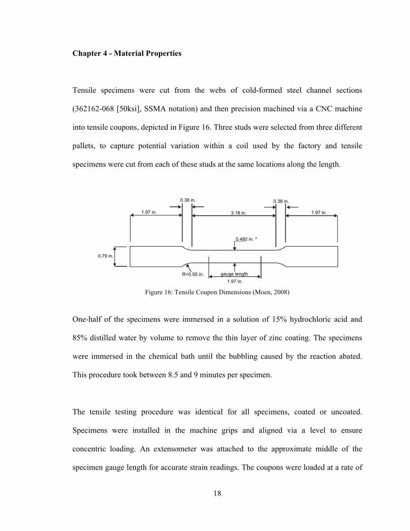
Chapter 4 - Material Properties
Tensile specimens were cut from the webs of cold-formed steel channel sections
(362162-068 [50ksi], SSMA notation) and then precision machined via a CNC machine
into tensile coupons, depicted in Figure 16. Three studs were selected from three different
pallets, to capture potential variation within a coil used by the factory and tensile
specimens were cut from each of these studs at the same locations along the length.
Figure 16: Tensile Coupon Dimensions (Moen, 2008)
One-half of the specimens were immersed in a solution of 15% hydrochloric acid and
85% distilled water by volume to remove the thin layer of zinc coating. The specimens
were immersed in the chemical bath until the bubbling caused by the reaction abated.
This procedure took between 8.5 and 9 minutes per specimen.
The tensile testing procedure was identical for all specimens, coated or uncoated.
Specimens were installed in the machine grips and aligned via a level to ensure
concentric loading. An extensometer was attached to the approximate middle of the
specimen gauge length for accurate strain readings. The coupons were loaded at a rate of
0.79 in.
1.97 in.
1.97 in.
3.18 in. 1.97 in.
0.38 in.0.38 in.
R=0.55 in.
0.492 in. *
gauge length
*nominal, actual dimension will vary slightly !"#$%&'!(!)!*'+,#-'!./%0/+!1#2'+,#/+,!34/'+!3(556778!
!
! *9'!,0'.#2'+,!:;<'&!.%<!='&'!#22'&,'1!#+!9>1&/.9-/&#.!:.#1?!./+.'+<&:<#/+!/;!@AB!#+!C/-%2'!
36AB!1#,<#--:<'1!=:<'&!:+1!@AB!9>1&/.9-/'!:.#17!;/&!@5!2#+%<',8!*9'!9>1&/.9-/'!D:<9!#,!+'.',,:&>!
</!&'2/C'!<9'!E#+.!./:<#+$!:+1!<9'+!D'!:D-'!</!2':,%&'!<9'!,0'.#2'+!1#2'+,#/+,!=#<9/%<!<9'!./:<#+$8!
"#$%&'!F!,9/=,!<9'!<',<!,'<!%0!:+1!/+'!/;!<9'!,0'.#2'+,!:;<'&!<',<'18!
!
! *=/!2'<9/1,!='&'!%,'1!</!;#+1!<9'!>#'-1#+$!,<&',,?!<9'!58(B!/;;,'<!2'<9/1!:+1!<9'!:%</$&:09!
2'<9/18!G:,#.:-->!<9'!58(B!2'<9/1!./+,#1'&!<9'!>#'-1#+$!,<&',,!'H%:-!</!<9'!,<&',,!=9'&'!<9'!,<#;;+',,!
-#+'!3I/%+$J,!2/1%-%,!K!L!K!(MA55N,#7!#,!/;;,'<!;&/2!<9'!/&#$#+!</!<9'!58(B!'+$#+''&#+$!,<&:#+!:+1!#<!
#+<'&,'.<!<9'!,<&',,O,<&:#+!.%&C'?!/+!<9'!/<9'&!9:+1?!<9'!:%</$&:09!2'<9/1!%,'!<9'!,:2'!/;;,'<!<'.9+#H%'!
D%<!<9'!-#+',!:&'!/;;,'<!</!58PB!:+1!586B!/;!<9'!,<&:#+!:+1!<9'!>#'-1#+$!,<&',,!#,!<9'!:C'&:$'!C:-%'!#+!<9'!
&:+$'!D'<=''+!<9'!<=/!-#+',8!
!
! Q--!<9'!1:<:!#,!1#,.&'<#E'1!:+1!$#C'+!#+!Q00'+1#R!S8!*9'!:%<9/&,!./+,#1'&!<9'!58(B!/;;,'<!2'<9/1!
<9'!2/,<!:00&/0&#:<'!2'<9/1!</!;#+1!<9'!>#'-1#+$!,<&',,!;/&!<9'!,<''-!%,'1!#+!<9'!,<%1,!D'.:%,'!<9'&'!#,!+/!
>#'-1#+$!0-:<':%!:,!,9/=+!#+!Q00'+1#R!T8!U+!<9'!/<9'&!9:+1?!<9'!,<''-!%,'1!#+!<9'!<&:.N!9:,!<9'!>#'-1#+$!
0-:<':%!:+1!<9'+!<9'!:%</$&:09!2'<9/1!#,!2/&'!:00&/0&#:<'V!#;!<9'!58(B!2'<9/1!#,!%,'1!</!1';#+'!<9'!
>#'-1#+$!,<&',,!<9'!C:-%'!=#--!D'!:!0':N!C:-%'!:,!,9/=+!#+!Q00'+1#R!W8!
!
:7!*',<!,'<O%0 D7!X/%0/+!;:#-'1!
"#$%&'!F!)!*'+,#-'!./%0/+!<',<8!
!

19
0.05 in/min for the first 1300 lbs. At this point, the loading rate was gradually slowed to
0.005 in/min to fully define the yield behavior. After the specimen had clearly passed the
yield point, the loading rate was restored to 0.05 in/min for the conclusion of the
experiment. All specimens were tested until failure. Figure 17 illustrates the test setup
and equipment utilized.
(a). Full experimental setup (b). Detail of extensomenter and specimen in
clamps Figure 17: Tensile Test Setup Depicting Equipment Used
Typical stress-strain curves for this specimen group are produced in Figure 18, with the
remainder of the response curves located in Appendix B: Tensile Results. Perhaps most
notable is the presence of a well-defined yield-plateau.

20
(a). Coated Specimen (b). Uncoated Specimen Figure 18: Stress-Strain curves with Superimposed 0.4% and 0.8% offset lines
The presence of the yield plateau governed the type of analysis method used to determine
specimen yield stress. The almost-archetypal 0.2% offset method is inappropriate for
tensile specimens demonstrating this yield behavior. Rather, the autographic method is
preferred as it better captures the plateau, utilizing two offset lines (0.4% and 0.8%) and
averaging their values to determine the yield stress.
Table 3 and Table 4 summarize the numeric results from the testing and tabulate
specimen average geometries. A complete table of specimen width and thickness
measurements is produced in Appendix C: Tensile Specimen Measurements of this report.
The yield and ultimate stresses demonstrate remarkably little variation, as opposed to the
ultimate engineering strain, which varies significantly. Similarly, while the zinc coating is
not observed to have any effect on the yield and ultimate stresses, uncoated specimens
experience much higher strains than coated specimens.

21
Table 3: Response Summary for Coated Specimens
Specimen # tave bave !u (in/in) Py (kip) Pu (kip) Fy* (ksi) Fu* (ksi)
s1c2 0.0745 0.4963 0.1865 2.24 2.86 60.7 77.3 s2c1 0.07296 0.4965 0.1261 2.16 2.83 59.5 78.1 s3c1 0.07308 0.4949 0.124 2.16 2.85 59.8 78.6 s3c3 0.0729 0.4954 0.1384 2.16 2.84 59.9 78.5
mean 0.14375 2.18 2.845 59.975 78.525
Fy* and Fu* are both calculated using coated thickness.
Table 4: Response Summary for Uncoated Specimens
Specimen# tave bave !u (in/in) Py (kip) Pu (kip) Fy (ksi) Fu (ksi)
s1c3 0.07152 0.4939 0.1542 2.14 2.84 60.7 80.3 s2c2 0.07158 0.4927 0.1363 2.09 2.76 59.2 78.2 s2c3 0.07162 0.4953 0.1554 2.11 2.8 59.5 78.9 s3c2 0.07154 0.4957 0.1895 2.13 2.82 60.2 79.6
mean 0.15885 2.12 2.805 59.9 79.25
It is hypothetical that this approximate 10% increase in strains is possibly due to the
stripping process removing small surface defects from the steel coupons. These small
defects can potentially expedite crack propagation, leading to less ductile failures. With
these removed, the specimen could experience greater ductility. However, a 10% increase
is not considered significant enough to warrant special consideration, especially
considering the limited number of tensile tests performed.
Another result of these coupon tests is the thickness of the galvanizing coating, reported in Table 5 and
Table 6. It is hypothesized that the difference in coating thickness between the specimen
groups (tested coated versus tested stripped) is due to rust that developed after coated
specimens were stripped. Furthermore, specimen s1c2 is perhaps an outlier, increasing
the average values for coated specimens. Measurements of the stripped metal for this

22
specimen group (tested while coated) were taken outside of the gauge length, so the strain
experience by the coupon was not a factor.
To determine yield stress in pre-rolled cold-formed sections, common practice is to cut
coupons from the section web or other large flat portion. The effect of cold work is
smaller in these locations, thus minimizing the influence of the manufacturing process
and yielding properties close to those of the virgin coil. Because this coupon is already
galvanized, one of two practices are employed to determine virgin coil properties: (1) test
the galvanized (coated) coupon and determine Pyc, the force at yield, then strip the
coupon after the test to determine base metal thickness and specimen width. The yield
stress is calculated as Fyc = Pyc/(ts bs). (2) strip the coupon and measure base metal width
and thickness. Test the stripped specimen and find the force at yield Pys. Yield stress is
calculated as Fys = Pys/(ts bs).
Results presented here predict a yield stress 1 to 2 ksi larger for specimens tested with their galvanizing
coating (described via Method 1) than those tested as stripped (Method 2). Surprisingly, if the test on the
galvanized coupon uses the coated thickness and width (tc and bc) in determination of the yield stress Fyc* =
Pyc/(tcbc), then Fyc* and Fys are found to be in very good agreement. Based on these findings, it is
recommended that method 2 (strip the specimen, measure properties, then test the specimen) should be the
standard method. Table 5 and
Table 6 compare stress values calculated using both stripped and coated steel thickness
values.
Table 5: Coating summary for specimens tested as coated
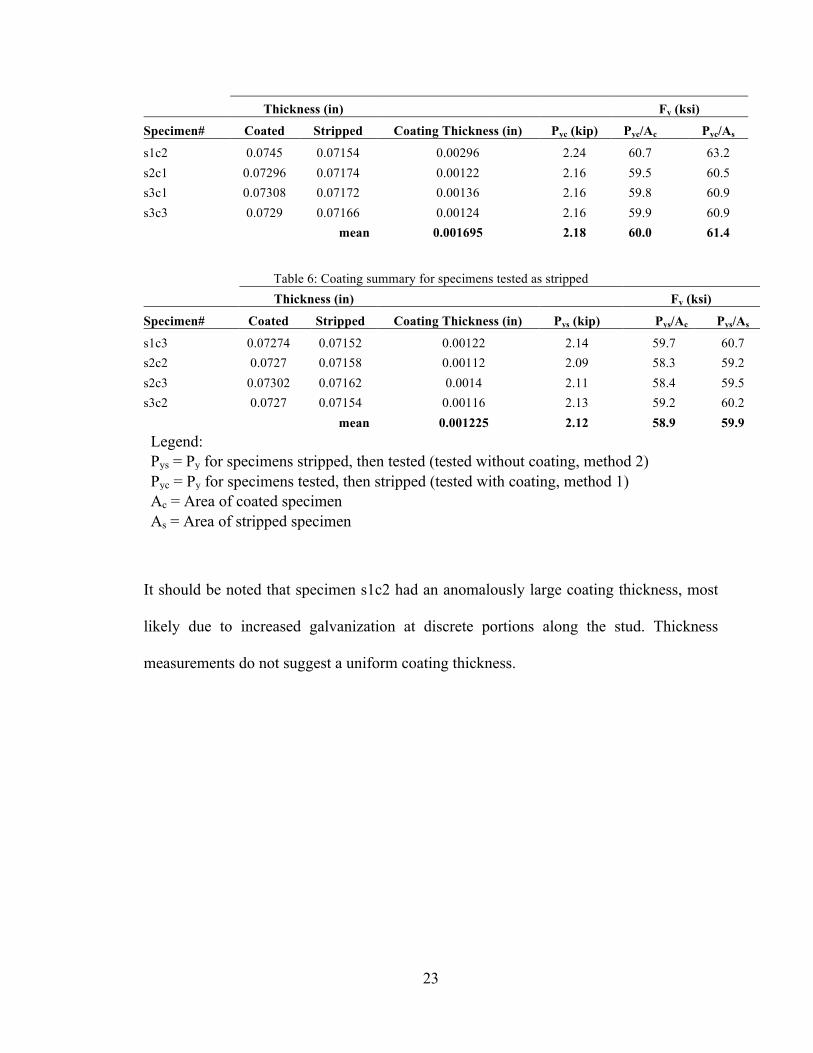
23
Thickness (in)
Fy (ksi)
Specimen# Coated Stripped Coating Thickness (in) Pyc (kip) Pyc/Ac Pyc/As
s1c2 0.0745 0.07154 0.00296 2.24 60.7 63.2 s2c1 0.07296 0.07174 0.00122 2.16 59.5 60.5 s3c1 0.07308 0.07172 0.00136 2.16 59.8 60.9 s3c3 0.0729 0.07166 0.00124 2.16 59.9 60.9
mean 0.001695 2.18 60.0 61.4
Table 6: Coating summary for specimens tested as stripped
Thickness (in)
Fy (ksi)
Specimen# Coated Stripped Coating Thickness (in) Pys (kip) Pys/Ac Pys/As
s1c3 0.07274 0.07152 0.00122 2.14 59.7 60.7 s2c2 0.0727 0.07158 0.00112 2.09 58.3 59.2 s2c3 0.07302 0.07162 0.0014 2.11 58.4 59.5 s3c2 0.0727 0.07154 0.00116 2.13 59.2 60.2
mean 0.001225 2.12 58.9 59.9
Legend: Pys = Py for specimens stripped, then tested (tested without coating, method 2)
Pyc = Py for specimens tested, then stripped (tested with coating, method 1) Ac = Area of coated specimen
As = Area of stripped specimen
It should be noted that specimen s1c2 had an anomalously large coating thickness, most
likely due to increased galvanization at discrete portions along the stud. Thickness
measurements do not suggest a uniform coating thickness.

24
Chapter 5 - Section
362S162-068 [50ksi] studs (SSMA notation) were utilized for this series of tests. Each
stud was measured at three locations along their length (corresponding approximately to
third-points) and dimensions were averaged across 40 measured specimens. The
following nomenclature, from Vieira 2011 (Figure 19) was adopted for consistency
across measurement programs in the same lab.
Figure 19: Adopted dimension nomenclature
Average dimensions are reported in Table 7, as well as nominal dimensions as reported in
the SSMA technical catalog. Dimensions for every specimen are reported in full in
Appendix E: Complete Cross-Section Measurements.
bB
h
bA
dB
dA
t
!hb-B
!hb-A !db-A
!db-B
rhb-B rdb-B
rhb-A rdb-A
Side B
Side A

Table 7: Average Dimensions across 40 Measured Studs (in)
Parameter Description Stud Side Nominal Measured % Difference h out-to-out web height --- 3.625 3.682 1.6 bA out-to-out-flange width A 1.625 1.699 4.6 bB out-to-out-flange width B 1.625 1.693 4.2 dA out-to-out lip height A 0.500 0.645 29.0 dB out-to-out lip height B 0.500 0.560 12.0 t Base metal thickness --- 0.0713 0.0715 0.28
rhb-B web-flange corner radius B 0.107 0.352 40.8 rdb-B flange-lip corner radius B 0.107 0.294 17.6 rhb-A web-flange corner radius A 0.107 0.348 39.2 rdb-A flange-lip corner radius A 0.107 0.306 22.4 "hb-B web-flange corner angle B 90 88.1 -2.1 "db-B flange-lip corner angle B 90 85.3 -5.2 "hb-A web-flange corner angle A 90 87.3 -3.0 "db-A flange-lip corner angle A 90 83.1 -7.7
Figure 33 depicts a representation of an idealized cross-section with listed SSMA
dimensions and a cross-section with the average measurements listed above.
26
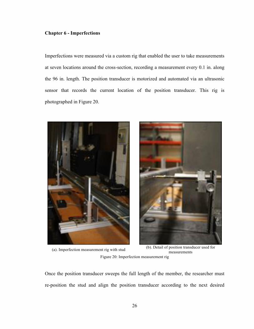
Chapter 6 - Imperfections
Imperfections were measured via a custom rig that enabled the user to take measurements
at seven locations around the cross-section, recording a measurement every 0.1 in. along
the 96 in. length. The position transducer is motorized and automated via an ultrasonic
sensor that records the current location of the position transducer. This rig is
photographed in Figure 20.
(a). Imperfection measurement rig with stud (b). Detail of position transducer used for
measurements Figure 20: Imperfection measurement rig
Once the position transducer sweeps the full length of the member, the researcher must
re-position the stud and align the position transducer according to the next desired
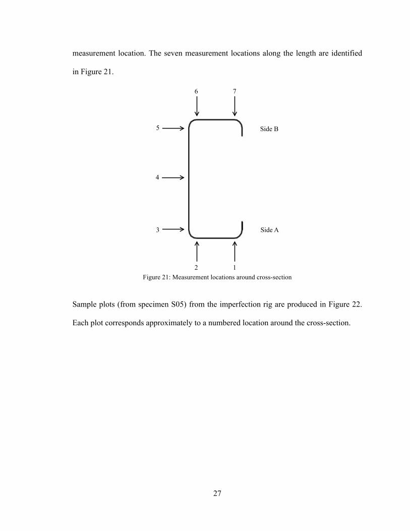
27
measurement location. The seven measurement locations along the length are identified
in Figure 21.
Figure 21: Measurement locations around cross-section
Sample plots (from specimen S05) from the imperfection rig are produced in Figure 22.
Each plot corresponds approximately to a numbered location around the cross-section.
7 6
5
4
3
1 2
Side B
Side A

28
Figure 22: Imperfection measurements for S05
100 90 80 70 60 50 40 30 20 10 00.1
0.05
0
0.05
0.1
Stud Length
Impe
rfect
ion
1
100 80 60 40 20 0 200.1
0.05
0
0.05
0.1
Stud Length
Impe
rfect
ion
2
100 90 80 70 60 50 40 30 20 10 00.4
0.45
0.5
0.55
0.6
0.65
Stud Length
Impe
rfect
ion
3
100 80 60 40 20 0 200.35
0.4
0.45
0.5
0.55
Stud Length
Impe
rfect
ion
4
100 80 60 40 20 0 20
0.35
0.4
0.45
0.5
0.55
0.6
Stud Length
Impe
rfect
ion
5
100 80 60 40 20 0 200.1
0.05
0
0.05
0.1
Stud Length
Impe
rfect
ion
6
100 80 60 40 20 0 200.1
0.05
0
0.05
0.1
Stud Length
Impe
rfect
ion
7
29
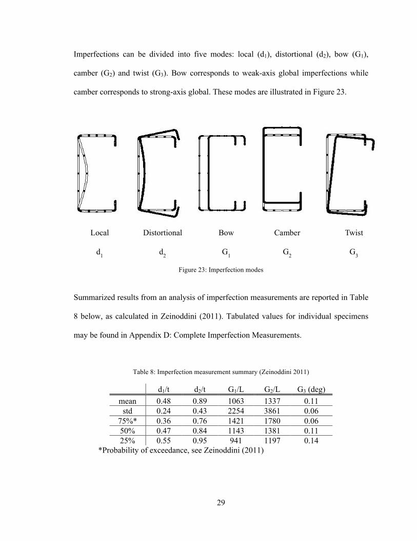
Imperfections can be divided into five modes: local (d1), distortional (d2), bow (G1),
camber (G2) and twist (G3). Bow corresponds to weak-axis global imperfections while
camber corresponds to strong-axis global. These modes are illustrated in Figure 23.
Figure 23: Imperfection modes
Summarized results from an analysis of imperfection measurements are reported in Table
8 below, as calculated in Zeinoddini (2011). Tabulated values for individual specimens
may be found in Appendix D: Complete Imperfection Measurements.
Table 8: Imperfection measurement summary (Zeinoddini 2011)
d1/t d2/t G1/L G2/L G3 (deg) mean 0.48 0.89 1063 1337 0.11 std 0.24 0.43 2254 3861 0.06
75%* 0.36 0.76 1421 1780 0.06 50% 0.47 0.84 1143 1381 0.11 25% 0.55 0.95 941 1197 0.14
*Probability of exceedance, see Zeinoddini (2011)
Local
d1
Distortional
d2
Bow
G1
Camber
G2
Twist
G3

Chapter 7 – Results
Table 9 (next page) summarizes results and failure modes for this test series and
compares results to those performed by Vieira (2011). A plot of the beam column tests in
the P-M space is represented in Figure 24.
Figure 24: Axial load (P) and mid-height horizontal load (H) at failure for 362S162-68 (50ksi) studs with
various sheathing configurations (B=Bare, O=OSB, G=Gypsum)
Photographic summaries of the various tests and limit states follow.
0 0.5 1 1.5 2 2.50
5
10
15
20
25
30
H horizontal load (kip)
P ax
ial lo
ad (k
ip)
OOGOOGGGOB or BOBB
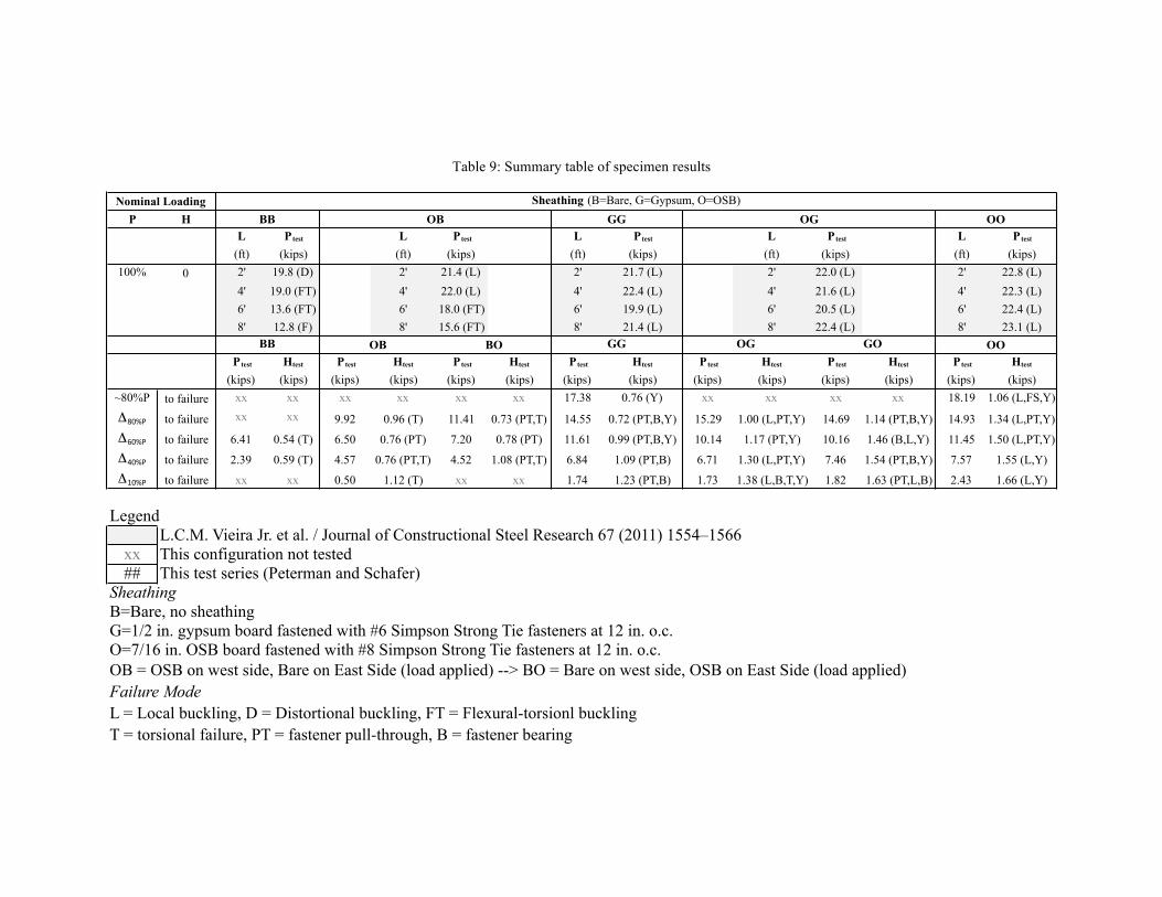
Table 9: Summary table of specimen results
Nominal Loading Sheathing (B=Bare, G=Gypsum, O=OSB)P H BB OB GG OG OO
L Ptest L Ptest L Ptest L Ptest L Ptest
(ft) (kips) (ft) (kips) (ft) (kips) (ft) (kips) (ft) (kips)100% 0 2' 19.8 (D) 2' 21.4 (L) 2' 21.7 (L) 2' 22.0 (L) 2' 22.8 (L)
4' 19.0 (FT) 4' 22.0 (L) 4' 22.4 (L) 4' 21.6 (L) 4' 22.3 (L)6' 13.6 (FT) 6' 18.0 (FT) 6' 19.9 (L) 6' 20.5 (L) 6' 22.4 (L)8' 12.8 (F) 8' 15.6 (FT) 8' 21.4 (L) 8' 22.4 (L) 8' 23.1 (L)
BB OB BO GG OG GO OOPtest Htest Ptest Htest Ptest Htest Ptest Htest Ptest Htest Ptest Htest Ptest Htest
(kips) (kips) (kips) (kips) (kips) (kips) (kips) (kips) (kips) (kips) (kips) (kips) (kips) (kips)~80%P to failure xx xx xx xx xx xx 17.38 0.76 (Y) xx xx xx xx 18.19 1.06 (L,FS,Y)
!!"#$ to failure xx xx 9.92 0.96 (T) 11.41 0.73 (PT,T) 14.55 0.72 (PT,B,Y) 15.29 1.00 (L,PT,Y) 14.69 1.14 (PT,B,Y) 14.93 1.34 (L,PT,Y)!%"#$ to failure 6.41 0.54 (T) 6.50 0.76 (PT) 7.20 0.78 (PT) 11.61 0.99 (PT,B,Y) 10.14 1.17 (PT,Y) 10.16 1.46 (B,L,Y) 11.45 1.50 (L,PT,Y)!&"#$ to failure 2.39 0.59 (T) 4.57 0.76 (PT,T) 4.52 1.08 (PT,T) 6.84 1.09 (PT,B) 6.71 1.30 (L,PT,Y) 7.46 1.54 (PT,B,Y) 7.57 1.55 (L,Y)!'"#$ to failure xx xx 0.50 1.12 (T) xx xx 1.74 1.23 (PT,B) 1.73 1.38 (L,B,T,Y) 1.82 1.63 (PT,L,B) 2.43 1.66 (L,Y)
LegendL.C.M. Vieira Jr. et al. / Journal of Constructional Steel Research 67 (2011) 1554–1566
xx This configuration not tested## This test series (Peterman and Schafer)
SheathingB=Bare, no sheathingG=1/2 in. gypsum board fastened with #6 Simpson Strong Tie fasteners at 12 in. o.c.O=7/16 in. OSB board fastened with #8 Simpson Strong Tie fasteners at 12 in. o.c. OB = OSB on west side, Bare on East Side (load applied) --> BO = Bare on west side, OSB on East Side (load applied)Failure ModeL = Local buckling, D = Distortional buckling, FT = Flexural-torsionl bucklingT = torsional failure, PT = fastener pull-through, B = fastener bearing
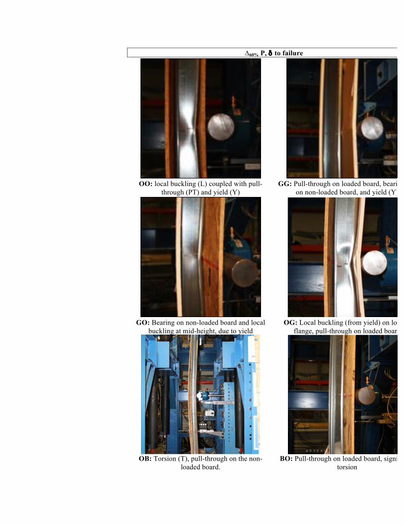
!60% P, ! to failure
OO: local buckling (L) coupled with pull-
through (PT) and yield (Y) GG: Pull-through on loaded board, bearing (B)
on non-loaded board, and yield (Y)
GO: Bearing on non-loaded board and local
buckling at mid-height, due to yield OG: Local buckling (from yield) on loaded
flange, pull-through on loaded board
OB: Torsion (T), pull-through on the non-
loaded board. BO: Pull-through on loaded board, significant
torsion

33
BB: Significant torsion (mid-height pictured)

34
!80% P, ! to failure
OO: Small local failure with slight pull-through on loaded board--member yield
GG: Pull-through on loaded board, bearing on non-loaded board, and yield
GO: Pull-through on loaded board, significant
torsion, bearing on non-loaded board, yield OG: Local failure at load point, pull-through
on loaded board and member yield
OB: Finite torsion, no pull-through BO: Torsion, pull-through on loaded board
35
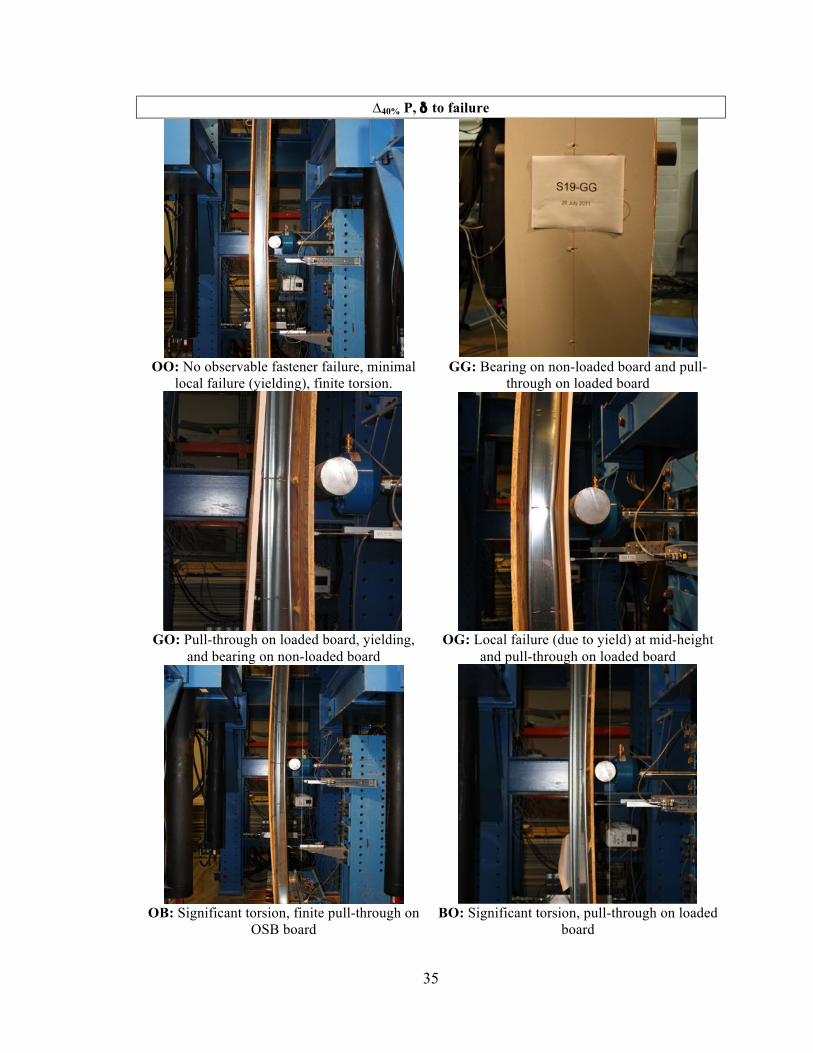
!40% P, ! to failure
OO: No observable fastener failure, minimal
local failure (yielding), finite torsion. GG: Bearing on non-loaded board and pull-
through on loaded board
GO: Pull-through on loaded board, yielding,
and bearing on non-loaded board OG: Local failure (due to yield) at mid-height
and pull-through on loaded board
OB: Significant torsion, finite pull-through on
OSB board BO: Significant torsion, pull-through on loaded
board

36
!10% P, ! to failure
OO: Local failure and member yield GG: Pull-through on loaded board and bearing
on non-loaded board
GO: Fastener pull-through on loaded board
and bearing on non-loaded board, local OG: Local failure (yield) and pull-through on
loaded board
OB: Significant torsion, no pull-through

37
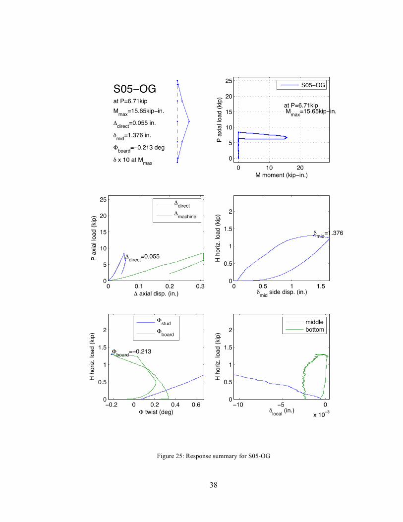
Post-processing of each specimen results in a series of plots based on raw sensor data and
designed to summarize the specimen response to loading. Figure 25 provides an example.
The upper left and upper right plots summarize loading and specimen response while the
remaining plots summarize sensor readings. Axial displacement measurements compare
string potentiometer readings to the direct readings from the MDOF rig. The horizontal
load vs. displacement plot simply tracks the loading of the specimen through the
horizontal load cell and the strain gauge within the load cell. The bottom left plot
compares stud twist (from the triplet sensors) to board twist, from sensors 5 and 6. The
bottom right plot charts the local displacement of the stud, as measured by the top and
bottom triplet sensors. Appendix H: Complete Specimen Response Summaries contains
summary plots for every specimen tested. Note, in these plots M=HL/8 is employed, i.e.
fixed end conditions are assumed in bending, this assumption is examined further in the
discussion section of this report.
38
Figure 25: Response summary for S05-OG
S05 OGat P=6.71kip
Mmax=15.65kip in.
direct=0.055 in.
mid=1.376 in.
board= 0.213 deg
x 10 at Mmax0 10 20
0
5
10
15
20
25
M moment (kip in.)
P a
xial
load
(kip
)
at P=6.71kip Mmax=15.65kip in.
S05 OG
0 0.1 0.2 0.30
5
10
15
20
25
axial disp. (in.)
P a
xial
load
(kip
)
direct=0.055
direct
machine
0 0.5 1 1.50
0.5
1
1.5
2
mid side disp. (in.)
H h
oriz
. loa
d (k
ip)
mid=1.376
0.2 0 0.2 0.4 0.60
0.5
1
1.5
2
twist (deg)
H h
oriz
. loa
d (k
ip)
board= 0.213
stud
board
10 5 0
x 10 3
0
0.5
1
1.5
2
local (in.)
H h
oriz
. loa
d (k
ip)
middlebottom

39
Each specimen type failed in different modes. The sections that follow compare the
sheathing types and how their response to load varies. One significant factor was the
difference in resistance to fastener bearing between OSB and gypsum. This component of
sheathing behavior largely governed the failure modes observed.
7.1 – OO Specimens
OSB sheathing was observed to be the strongest against bearing. In the case of double-
sided OSB sheathed specimens, stud twist was resisted on both side of the stud, leading
to a localized buckling failure with slight pull-through without significant observable
torsion (Figure 26b).
(a). Side view of failure (b). Close-up of localized failure
Figure 26: S38-OO
40
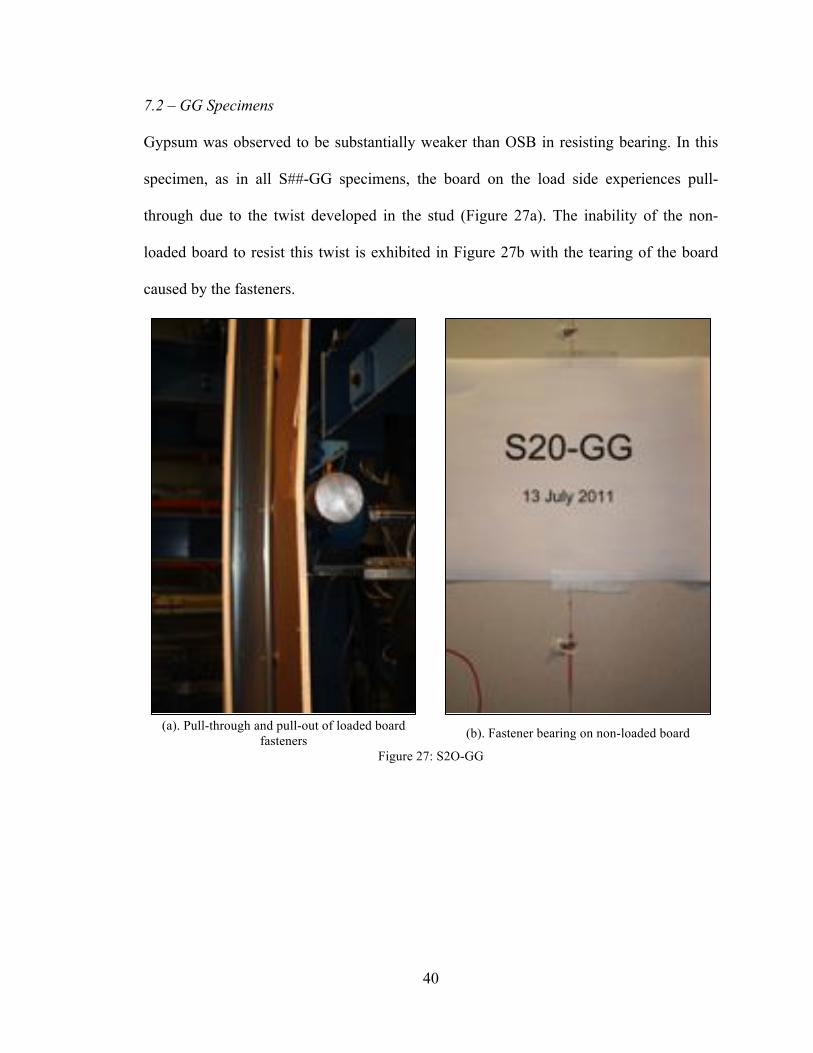
7.2 – GG Specimens
Gypsum was observed to be substantially weaker than OSB in resisting bearing. In this
specimen, as in all S##-GG specimens, the board on the load side experiences pull-
through due to the twist developed in the stud (Figure 27a). The inability of the non-
loaded board to resist this twist is exhibited in Figure 27b with the tearing of the board
caused by the fasteners.
(a). Pull-through and pull-out of loaded board
fasteners (b). Fastener bearing on non-loaded board
Figure 27: S2O-GG

41
7.3 – GO Specimens
Dissimilarly sheathed columns proved interesting in that they permitted the effect of load
face to take effect. With weaker gypsum on the non-loaded face and OSB on the loaded
face, the stud twisted due to the low bearing resistance of the gypsum (Figure 28c). The
front board, OSB, remained entirely intact, with little evidence of fastener pull-through
(Figure 28a).
(a). Intact OSB board post-failure (b). Side view of failure
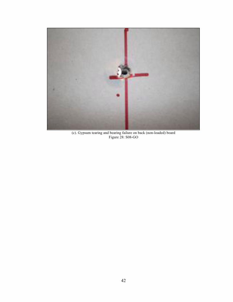
42
(c). Gypsum tearing and bearing failure on back (non-loaded) board
Figure 28: S08-GO

43
7.4 – OB Specimens
Columns with one side left bare demonstrated highly unpredictable responses, as seen in
Figure 24. Loading the stud directly is neither realistic nor generalizable over different
loading scenarios. In these specimens, the OSB board restrained the stud from twist only
slightly. Because the resistance to torsion is so low for bare specimens, the fasteners in
the OSB back board showed evidence of pull-though.
(a). Side view of failure (b). Fastener pull-through
Figure 29: S14-OB

44
7.5 – BO Specimens
With no non-loaded board to aid in restricting twist and a shear-resistant front board,
S##-BO specimens responded to torsion demands by twisting significantly, as seen in
Figure 30a and Figure 30b. The OSB on the load face resisted fastener pull-through and
shear forces, as neither of these behaviors were observed. Despite the large magnitude of
twist, after unloading, the stud elastically deformed to its original position (Figure 30c).
(a). Back view, stud failure

45
(b). Detail demonstrating magnitude of twist at peak load
(c). Detail of elastic behavior after unloading
Figure 30: S27-BO

46
7.6 – BB Specimens
Columns without any sheathing at all simply twisted until failure, shown in Figure 31.
Because of this twist, in extreme instances, the load bar applied load on the beginning of
the web face, rather than the flange face. In a testament to the end conditions, stud ends
remained torsionally fixed despite extraordinary amounts of twist in the stud middle
(Figure 31b).
(a). Back view of stud failure, demonstrating twist magnitude
(b). Detail of stud ends at peak horizontal load—note torsional fixity despite significant twist at mid-height
Figure 31: S26-BB
47
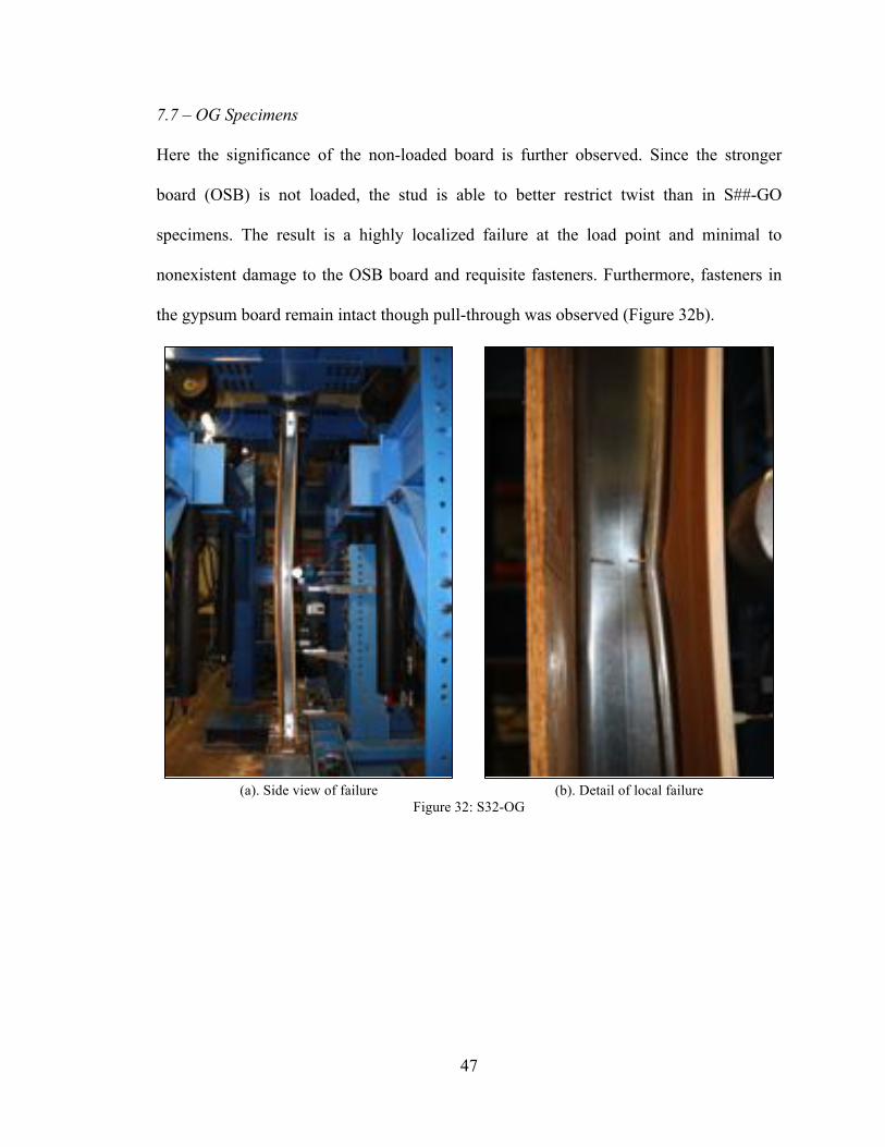
7.7 – OG Specimens
Here the significance of the non-loaded board is further observed. Since the stronger
board (OSB) is not loaded, the stud is able to better restrict twist than in S##-GO
specimens. The result is a highly localized failure at the load point and minimal to
nonexistent damage to the OSB board and requisite fasteners. Furthermore, fasteners in
the gypsum board remain intact though pull-through was observed (Figure 32b).
(a). Side view of failure (b). Detail of local failure
Figure 32: S32-OG

48
Chapter 8 – Nominal Capacity Analysis
This chapter provides member and fastener capacities that later may be used to compare
to the testing. The direct comparison to the testing requires some consideration of the end
conditions and the manner in which the fasteners are loaded – these issues are taken up in
Section 8 where the comparisons are provided, this section just provides basic capacity.
Figure 33 CUFSM models, drawn to scale, used for cross-section elastic buckling analysis (note, t=0.0715 in. and Fy= 59.9 ksi in the as-measured sections for this study, while t=0.0656 in. and Fy=55.5 ksi for the
as-measured of Vieira et al., see Section 3 and 4 of this report for full details of the as-measured dimensions for this study)
8.1 Local Buckling Member Capacity
The upper bound capacity of the sheathed stud is the local buckling capacity. In the axial
load tests of Vieira (2011) local buckling controlled the strength. If it is presumed that
only local buckling controls (note this is not the case in the observed tests as fastener
limit states and torsion were generally observed, but this is the upper bound strength),
then: check only local buckling, i.e., no distortional buckling, no global buckling, no
torsion, and no fastener failure. Under these assumptions Cm=1 and "=1, therefore a
362S162 68 Nominal As measured (this study) As measured Vieira et al.

49
simplified version of the AISI-S100 interaction equations (C5.2) may be used, which at
nominal capacities and loads implies
where P and M are the demands and Pn and Mn are the capacities for only local buckling.
AISI-S100-07 provides an Effective Width approach in the main Specification (largely,
Chapter B) and the Direct Strength approach in the Appendix (Appendix 1). Under the
preceding assumptions Pn and Mn may be found as follows:
Pn, main spec AISI S100 = Pno per C5.2 App. 1 DSM AISI S100 = Pn! with Pne=Py per App. 1 1.2.1.2 Mn, Main spec AISI S100 = Mn per C3.1.1(a) App. 1 DSM AISI S100 = Mn! with Mne=My per App. 1 1.2.2.2
Table 10 provides Pn and Mn for the nominal and as-measured dimensions and properties.
Table 10 Capacity of 362S162-68 (50 ksi) for LOCAL BUCKLING
Capacity in Compression and Bending6 dimensions and properties based on
Provision
Nominal
Peterman and Schafer Beam-column tests
As-measured
Vieira et al. Axial only tests As-measured
Pn Main Spec. 20.2 kips1 -5 -5 DSM (App. 1) 23.7 kips2 28.0 kips3 22.2 kips4
Mn Main Spec 28.7 in.-kips1 -5 -5 DSM (App. 1) 29.5 in.-kips2 34.5 in.-kips3 30.6 in.-kips4
1 AISI (2008) Table III-2 for Pn and AISI (2008) Table II-2 for Mn 2 Ag=0.524 in2, Sg=0.590 in3 per SSMA (2010), Pcr! = 31.7 kip, Mcr! = 152.6 in.-kips per CFSEI G103-11 (2011), Pn and Mn found per AISI-S100-07 Appendix 1. 3 t=0.0715in., Ag=0.522 in2, Sg=0.577 in3, Fy=59.9ksi, Pcr! = 36.8 kip, Mcr! = 196.9 in.-kips per CUFSM model of as-measured properties, Pn and Mn per AISI-S100-07 App. 1. 4 t=0.0656in., Ag=0.484 in2, Sg=0.5552 in3, Fy=55.5ksi, Pcr! = 24.7 kip, Mcr! = 122.5 in.-kips per CUFSM model of as-measured properties, Pn and Mn per AISI-S100-07 App. 1. 5 Not calculated. 6 for nominal dimensions and properties note that Pnd and Mnd (per AISI 2008 Tables II-8 and III-5) are greater than Pn and Mn (for local buckling only) even with k#=0, so distortional buckling does not control.
PPn+MMn
!1

50
8.2 Sheathing Braced Member Capacity
Member capacity is controlled by local, distortional, or global buckling (and/or
combinations thereof). As discussed in detail in Vieira (2011) these buckling modes,
particularly global buckling, may be influenced greatly by the presence of sheathing.
Here we consider local buckling, distortional buckling, global buckling, but no direct
torsion, and no fastener failure. Further we ignore the small second order amplification,
therefore Cm=1 and "=1, and again a simplified version of the AISI-S100 interaction
equations (C5.2) may be used, which at nominal capacities and loads implies
where P and M are the demands and Pn and Mn are the capacities, considering local,
distortional, and global buckling. This is accomplished by determined the elastic critical
local, distortional, and global buckling modes with appropriate springs modeling the
fastener-sheathing stiffness. The approach can be modified for use in the main
Specification of AISI-S100-07, but more easily follows from the Direct Strength
approach in the Appendix (Appendix 1). Under the preceding assumptions Pn and Mn
may be found as follows:
Pn, App. 1 DSM AISI S100 with Pcr!, Pcrd, Pcre including sheathing springs Mn, App. 1 DSM AISI S100 with Pcr!, Pcrd, Pcre including sheathing springs
The crucial step in the strength calculation via AISI-S100 Appendix 1 (Direct Strength) is
the determination of the elastic buckling loads. This may be most easily accomplished
with a finite strip analysis, using software such as CUFSM. CUFSM also provides a
means to include the impact of springs. Based on the work of Vieira (2011) the stud-
PPn+MMn
!1

51
fastener-sheathing spring stiffness has previously been determined and is reported in
Figure 34.
Figure 34 Fastener-sheathing stiffness (k’s) for OSB and Gypsum, converted to foundation stiffness (k’s)
The foundation stiffness values are included in a CUFSM 4.04 model of each of the
cross-sections (Figure 33) and models are completed for both pinned and fixed end
conditions with all sheathing configurations as reported in Table 11. In addition the
elastic buckling values are used to determine the predicted capacity based on member
buckling limit states via AISI-S100 Appendix 1 (Direct Strength Method) and also
reported in Table 11.
The results of Table 11 are extensive and the strength predictions will be evaluated
further in Section 8; however, some items are worth noting.
• Overall the predicted strengths show similar progression in capacities as a
function of sheathing as the testing.
• The presence of two-sided sheathing, whether it be gypsum board, OSB, or one of
each greatly increases the predicted member capacities and even, to some extent,
minimizes the importance of the end boundary conditions.
kx ky
k!"
kx ky
k!"
sheathing spring stiffness1 conversion to imperial foundation stiffness for CUFSM2
OSB kx 971 N/mm 5.52 kip/in. kx 0.46 kip/in./in." ky 0.374 N/mm 0.0021 kip/in. ky 0.00018 kip/in./in." kf 95309 Nmm/rad 0.84 kip-in./rad kf 0.070 kip-in./rad/in.
Gyp kx 427 N/mm 2.43 kip/in. kx 0.20 kip/in./in." ky 0.087 N/mm 0.00049 kip/in. ky 0.000041 kip/in./in." kf 95987 Nmm/rad 0.85 kip-in./rad kf 0.071 kip-in./rad/in.
(1) source: Vieira (2011) Table 6.3, fastener-stud-sheathing nominal dimensions and properties same as this testing(2) as reported in Vieira (2011), fastener spacing of 12 in. used to convert to foundation stiffness for use in CUFSM
52
• The predicted strength differences between the nominal cross-section and the as-
measured cross-sections can be large.
• Though not specifically noted on the table, for pinned end conditions in
compression when two-sided sheathing is present the controlling global buckling
mode is strong-axis buckling of the stud, thus one would consider the sheathing
has successfully restricted weak-axis buckling and torsional(-flexural) buckling.
• For the 362S162-68 (50ksi) as a beam, local and distortional buckling should not
control, instead global buckling is essentially the only relevant mode. (Note, the
predictions do not include inelastic bending reserve, which may provide a modest
boost to the predicted capacities in local and distortional buckling).

53
Table 11 Nominal member capacity analysis including sheathing (using AISI-S100 Appendix 1 DSM)
8.3 Fastener/Connection limit state capacities
Fastener shear and tensile capacity
Fastener nominal shear (Pss) and tensile (Pts) capacity is available: Simpson Quikdrive No.
6 x 1!” fasteners as used for attaching gypsum, Pss=1260 lbf, Pts=1720 lbf; Simpson
Quikdrive No. 8 x 1 15/16” as used for attaching the OSB, Pss=1565 lbf, Pts=2160 lbf (per
http://www.strongtie.com/products/fasteners/quikdrive_general_load_tables.html).
AXIAL BENDINGPy Pcrl/Py Pcrd/Py Pcre/Py Pn
1 My Mcrl/My Mcrd0/My Mcre0/My CbMcre0/My Mn2
section end cond. sheathing sheathing (kips) (kips) sheathing (kip-in.) (kip-in.)nominal pinned bare BB 26.2 1.21 1.47 0.22 5.1 BB 29.4 5.08 2.67 0.41 0.54 16.0
" " one-sided OB/BO 26.2 1.21 1.51 0.49 11.1 OB 29.4 >5.08 >2.67 0.93 1.23 25.3" " " BO 29.4 >5.08 >2.67 >10 >10 29.4" " two-sided GG 26.2 1.21 1.55 1.21 18.5 GG 29.4 >5.08 >2.67 >10 >10 29.4" " " OG/GO 26.2 1.21 1.56 1.24 18.7 OG 29.4 >5.08 >2.67 >10 >10 29.4" " " GO 29.4 >5.08 >2.67 >10 >10 29.4
" " " OO 26.2 1.21 1.56 1.26 18.8 OO 29.4 >5.08 >2.67 >10 >10 29.4" fixed bare BB 26.2 1.21 1.49 0.68 14.2 BB 29.4 >5.08 >2.67 1.38 1.82 27.7" " one-sided OB/BO 26.2 1.21 1.54 0.99 17.1 OB 29.4 >5.08 >2.67 1.72 2.27 28.7" " " BO 29.4 >5.08 >2.67 >10 >10 29.4" " two-sided GG 26.2 1.21 1.57 2.83 21.4 GG 29.4 >5.08 >2.67 >10 >10 29.4" " " OG/GO 26.2 1.21 1.58 3.02 21.5 OG 29.4 >5.08 >2.67 >10 >10 29.4" " " GO 29.4 >5.08 >2.67 >10 >10 29.4" " " OO 26.2 1.21 1.58 3.50 21.8 OO 29.4 >5.08 >2.67 >10 >10 29.4
as-measured pinned bare BB 31.3 1.17 1.28 0.19 5.2 BB 35.5 5.70 2.35 0.37 0.48 17.1Peterman & " one-sided OB/BO 31.3 1.17 1.32 0.41 11.2 OB 35.5 >5.70 >2.35 0.80 1.06 29.1
Schafer " " BO 35.5 >5.70 >2.35 >8 >8 35.5" " two-sided GG 31.3 1.17 1.35 1.01 20.7 GG 35.5 >5.70 >2.35 >8 >8 35.5" " " OG/GO 31.3 1.17 1.35 1.02 20.7 OG 35.5 >5.70 >2.35 >8 >8 35.5" " " GO 35.5 >5.70 >2.35 >8 >8 35.5" " " OO 31.3 1.17 1.36 1.04 20.9 OO 35.5 >5.70 >2.35 >8 >8 35.5" fixed bare BB 31.3 1.17 1.30 0.58 15.2 BB 35.5 >5.70 >2.35 1.23 1.63 32.8" " one-sided OB/BO 31.3 1.17 1.34 0.86 19.2 OB 35.5 >5.70 >2.35 1.52 2.00 34.0" " " BO 35.5 >5.70 >2.35 >8 >8 35.5" " two-sided GG 31.3 1.17 1.38 2.37 24.8 GG 35.5 >5.70 >2.35 >8 >8 35.5" " " OG/GO 31.3 1.17 1.38 2.56 25.0 OG 35.5 >5.70 >2.35 >8 >8 35.5" " " GO 35.5 >5.70 >2.35 >8 >8 35.5" " " OO 31.3 1.17 1.39 2.92 25.4 OO 35.5 >5.70 >2.35 >8 >8 35.5
as-measured pinned bare BB 26.9 0.91 1.17 0.20 4.7 BB 30.6 3.99 2.18 0.37 0.49 15.0Vieira et al. " one-sided OB/BO 26.9 0.91 1.21 0.44 10.4 OB 30.6 >3.99 2.18 0.83 1.10 25.5(axial only) " " BO 30.6 >3.99 2.30 >11 >11 30.6
" " two-sided GG 26.9 0.91 1.25 1.13 17.3 GG 30.6 >3.99 >2.30 >11 >11 30.6" " " OG/GO 26.9 0.91 1.25 1.15 17.3 OG 30.6 >3.99 >2.30 >11 >11 30.6" " " GO 30.6 >3.99 >2.30 >11 >11 30.6" " " OO 26.9 0.91 1.26 1.16 17.4 OO 30.6 >3.99 >2.30 >11 >11 30.6" fixed bare BB 26.9 0.91 1.19 0.62 13.7 BB 30.6 >3.99 2.21 1.27 1.68 28.4" " one-sided OB/BO 26.9 0.91 1.23 0.90 16.2 OB 30.6 >3.99 >2.21 1.57 2.08 29.5" " " BO 30.6 >3.99 >2.21 >11 >11 30.6" " two-sided GG 26.9 0.91 1.27 2.62 19.9 GG 30.6 >3.99 >2.21 >11 >11 30.6" " " OG/GO 26.9 0.91 1.28 2.75 20.0 OG 30.6 >3.99 >2.21 >11 >11 30.6" " " GO 30.6 >3.99 >2.21 >11 >11 30.6" " " OO 26.9 0.91 1.28 3.21 20.3 OO 30.6 >3.99 >2.21 >11 >11 30.6
(1) calculated per AISI-S100-07 Appendix 1 (DSM) with appropriate kx, ky, kf springs included in CUFSM4 models for finding Pcrl, Pcrd, Pcre (2) calculated per AISI-S100-07 Appendix 1 (DSM) with appropriate kx, ky, kf springs included in CUFSM4 models for finding Mcrl, Mcrd, Mcre (3) the number of longitudinal (m) terms kept in the CUFSM runs is as follows
nominal 1-10,33-39 for P runs 1-12,45-51 for M runsas-measured 1-10,31-37 for P runs 1-11,39-45 for M runsVieira et al. 1-10,33-39 for P runs 1-11,44-50 for M runs
54
Pull-through
Exact pull-through values are not directly available. For the Simpson WSNTL screw in
7/16 in. OSB (this screw is similar to the PPSD screw employed here, but not identical)
the allowable pull-through is 70 lbf with a safety factor of 5; the nominal pull-through =
350 lbf. (http://www.strongtie.com/products/fasteners/WSNTL.html).
The authors are unaware of published pull-through capacities for gypsum board; however
withdrawal values for nails are provided by the Gypsum Association, treating these as a
lower bound, the nominal pull-through in gypsum board is 80 lbf. (per GA-235-10,
Gypsum Board Typical Mechanical and Physical Properties.)
An alternative source of pull-through values are the rotational restraint tests of Vieira
(2011). The tests as illustrated in Figure 35 were conducted on the same stud, fastener,
and sheathing combinations as examined here, specifically: two types of sheathing are
employed: OSB (7/16 in., rated 24/16, exposure 1) and gypsum (1/2 in. Sheetrock). Five
Number 6 screws (Simpson #6 x 1 5/8’’) spaced 12 in. apart on a 54 in. wide board were
used to connect to the gypsum boards and the same spacing and board width with number
8 screws (Simpson #8 x 1 15/16’’) were used to connect to the OSB boards. The boards
were kept in an environmental chamber for seven days at a temperature of 20 C and 65%
humidity. Maximum capacities were not reported in Vieira (2011) or the resulting paper
(Schafer et al. 2009) so that data is provided here in Figure 36.

55
The moment (M) at which the fasteners pulled through (the observed failure mode in the
rotational restraint test) is divided by the board width (w) and recorded as the Moment
per unit width (M) in Figure 36. In the test M is equilibrated by 5 fasteners that create
their own moment resisting couples consisting of pull-through at the fastener (Ppt) and an
equal and opposite bearing force at the flange/web juncture half the flange width (0.5b)
away; therefore:
M =Mw = 5 !Ppt 12 b therefore Ppt = 2Mw / 5b( )
Using the average M values from the testing reported in Figure 36 and noting w=54 in.
and b = 1.62 in., then Ppt_OSB = 437 lbf, and Ppt_gyp = 40 lbf. (Note, the gypsum board has
significant variation if the high M first test is thrown out as an outliner Ppt_gyp = 25 lbf).
Bearing
Bearing values are available for the tested configurations (stud, fastener, and sheathing)
in Vieira (2011). Nominal bearing capacity (Pbr) for #8’s anchored in a 68 mil stud
through 7/16 in. OSB is 578 lb (2572 N from Table 3.2 in Vieira 2011) and for #6’s
anchored in a 68 ml stud through " in. Gypsum is 86 lbf (382 N).
Fastener limit state summary
Table 12 Summary of fastener-sheathing limit state capacities #8 in OSB #6 in Gypsum Pss, Fastener shear1 1565 lbf 1260 lbf Pts, Fastener tension1 2160 lbf 1720 lbf Ppt, Pull-through2 437 lbf 40 lbf Pbr, Bearing3 578 lbf 86 lbf 1. Based on industry reported value, 2. Based on rotational restraint test, 3. Based on translational stiffness testing

56
Figure 35 Rotational restraint test as reported in Schafer et al. (2009), this test provides a pull-through
failure mode comparable to the pull-through observed in the axial testing herein.
Figure 36 Moment-rotation from rotational restraint tests reported in Schafer et al. (2009) (Note, paper only reported stiffness, here the moment/length is provided as well, this plot has not been previously reported).
0 0.5 10
1
2
3
4
5
6
7
8BBB GYP 12 6 6 01.dat
k = 77 lbf in./in./rad
Mmax = 6.3 lbf in./in.
(rad)
Mom
ent (
lbf
in./i
n.)
0 0.5 10
1
2
3
4
5
6
7
8BBB GYP 12 6 6 03.dat
k = 67 lbf in./in./rad
Mmax = 1.5 lbf in./in.
(rad)
Mom
ent (
lbf
in./i
n.)
0 0.5 10
1
2
3
4
5
6
7
8BBB GYP 12 6 6 04.dat
k = 79 lbf in./in./rad
Mmax = 2.3 lbf in./in.
(rad)
Mom
ent (
lbf
in./i
n.)
0 0.5 10
1
2
3
4
5
6
7
8BBB GYP 12 6 6 05.dat
k = 52 lbf in./in./rad
Mmax = 2.0 lbf in./in.
(rad)
Mom
ent (
lbf
in./i
n.)
0 0.5 1 1.50
5
10
15
20
25
30
35
40BBB OSB 12 8 6 02.dat
k = 103 lbf in./in./rad
Mmax = 33.9 lbf in./in.
(rad)
Mom
ent (
lbf
in./i
n.)
0 0.5 1 1.50
5
10
15
20
25
30
35
40BBB OSB 12 8 6 06.dat
k = 85 lbf in./in./rad
Mmax = 31.3 lbf in./in.
(rad)
Mom
ent (
lbf
in./i
n.)
0 0.5 1 1.50
5
10
15
20
25
30
35
40BBB OSB 12 8 6 07.dat
k = 86 lbf in./in./rad
Mmax = 31.7 lbf in./in.
(rad)
Mom
ent (
lbf
in./i
n.)
0 0.5 1 1.50
5
10
15
20
25
30
35
40BBB OSB 12 8 6 08.dat
k = 91 lbf in./in./rad
Mmax = 34.2 lbf in./in.
(rad)
Mom
ent (
lbf
in./i
n.)

57
Chapter 9 – Discussion
9.1 - Load Location
As briefly discussed in Section 1.6, the location of where the horizontal force H is
applied to the specimen cross-section changes with the amount the stud twists. The bar
begins loading at approximately the center of the flange. With a finite amount of twist,
the bar remains on the flat width of the flange, but closer to the web-flange corner (Figure
37b). As this twist increases, however, the stud twists such that the bar applies load to the
web-flange corner (Figure 37c). Determining torsional stresses on this cross-section can
be convoluted in this instance, as the relationship of the load to stud shear center has
dramatically changed.
In the case of OX specimens (sheathed with OSB on the non-loaded face), the OSB
restricts stud twist on the non-loaded face, resulting in a deformed cross-section with
non-uniform twist (Figure 37d). For the other specimen types, the deformed cross-section
varies modestly as well, for example in the OG and GO cases.

58
Figure 37: Load location cases (a) initial position (b) finite twist (c) large twist (d) OX case
Despite this complexity, for any small, but finite twist, the authors suggest assuming a
load location at the end of the flange flat width, nearest to the web-flange corner (Figure
37b) this is also consistent with studs directly loaded under small, but finite twist (see
Figure 15b). So, e = m + t/2 + r, where e is the eccentricity of the load from the shear
center, m is the distance from the shear center to the mid-plane of the web (as commonly
tabled by SSMA, etc.) t is the design thickness, and r is the inner radius.
For nominal dimensional properties of a 362S162-68:
e = m + t/2 + r = 0.765 in. + 0.0713 in./2 + 0.1070 in. = 0.91 in.
9.2 - End Conditions
To accurately resolve the applied horizontal load into moments in the specimen, it is
necessary to characterize the specimen end conditions. The intent of the detailed stud end
conditions (see Section 1.3) was to simulate a stud in a complete wall system and the
expectation, after previously conducted axial testing (Vieira 2011), was that this would
(a) (b) (c) (d)
H (resultant) e
shear center

59
supply fixed ends. Although the intent was met and the authors believe the stud-to-track-
to-sheathing end condition is close to actual field conditions, the expectation of fixed end
conditions was not met as the situation for members in bending is more complicated than
members in compression.
A direct examination of the horizontal displacements of the studs at failure provides a
preliminary indication of the role of the axial load in restricting the rotations at the ends.
Figure 38 shows a series of OO sheathed specimens as the axial load is decreased before
applying horizontal load to failure. (The OO specimens are selected because the exhibit
little torsion and thus the horizontal displacements may be accurately understood as
emanating directly from bending and not a horizontal component of the torsion itself.)
For Figure 38a (with axial load near 80% of its axial capacity, i.e. “80%P”) it is clear that
the displacements near the member ends are minimized and some end fixity is present;
however, at “10%P” no such fixity is observed in the sensor data.
(a) (b) (c)
Figure 38: Summary results and measured specimen horizontal displacement for OO sheathed specimens with decreasing axial load (a) “80%P”, (b) 60% P, (c) 10%P
S15 OOat P=14.93kipHmax=1.34kip
direct=0.083 in.
mid=1.069 in.
board=0.363 deg
x 10 at Hmax0 0.5 1
0
5
10
15
20
25
H horizontal load (kip)
P ax
ial l
oad
(kip
)
at P=14.93kip Hmax=1.34kip in.
S15 OO
0 0.1 0.2 0.3 0.40
5
10
15
20
25
axial disp. (in.)
P ax
ial l
oad
(kip
)
direct=0.083
direct
machine
0 0.5 10
0.5
1
1.5
2
mid side disp. (in.)
H h
oriz
. loa
d (k
ip)
mid=1.069
0 0.2 0.4 0.60
0.5
1
1.5
2
twist (deg)
H h
oriz
. loa
d (k
ip)
board=0.363
stud
board
15 10 5 0 5x 10 3
0
0.5
1
1.5
2
local (in.)
H h
oriz
. loa
d (k
ip)
middlebottom
S38 OOat P=11.45kipHmax=1.50kip
direct=0.062 in.
mid=1.138 in.
board= 0.807 deg
x 10 at Hmax0 0.5 1 1.5
0
5
10
15
20
25
H horizontal load (kip)
P ax
ial l
oad
(kip
)
at P=11.45kip Hmax=1.50kip in.
S38 OO
0 0.1 0.2 0.3 0.40
5
10
15
20
25
axial disp. (in.)
P ax
ial l
oad
(kip
)
direct=0.062
direct
machine
0 0.5 1 1.50
0.5
1
1.5
2
mid side disp. (in.)
H h
oriz
. loa
d (k
ip)
mid=1.138
0.8 0.6 0.4 0.2 0 0.2 0.40
0.5
1
1.5
2
twist (deg)
H h
oriz
. loa
d (k
ip)
board= 0.807
stud
board
15 10 5 0 5x 10 3
0
0.5
1
1.5
2
local (in.)
H h
oriz
. loa
d (k
ip)
middlebottom
S11 OOat P=2.43kipHmax=1.66kip
direct=0.034 in.
mid=1.605 in.
board= 0.808 deg
x 10 at Hmax0 0.5 1 1.5
0
5
10
15
20
25
H horizontal load (kip)
P ax
ial l
oad
(kip
)
at P=2.43kip Hmax=1.66kip in.
S11 OO
0 0.05 0.1 0.150
5
10
15
20
25
axial disp. (in.)
P ax
ial l
oad
(kip
)
direct=0.034
direct
machine
0 0.5 1 1.50
0.5
1
1.5
2
mid side disp. (in.)
H h
oriz
. loa
d (k
ip)
mid=1.605
0.8 0.6 0.4 0.2 0 0.2 0.40
0.5
1
1.5
2
twist (deg)
H h
oriz
. loa
d (k
ip)
board= 0.808
stud
board
10 5 0x 10 3
0
0.5
1
1.5
2
local (in.)
H h
oriz
. loa
d (k
ip)
middlebottom

60
To more definitively quantify the end boundary conditions the horizontal force (H) vs.
the measured mid-height displacement (!) was compared against theoretical fixed, pinned,
and semi-rigid solutions in Figure 39. The theoretical fixed and pinned solutions are:
fixed: ! = HL3 / (192EI ), k =192EI / L3 pinned: ! = HL3 / (48EI ), k = 48EI / L3
where nominal dimensions are employed for EI. The results (Figure 42) indicate that
even under significant axial load the boundary conditions for bending about the major-
axis of the stud are not fixed. In fact, for all cases pinned end boundary conditions are a
more accurate estimate of the observed stiffness.
(a) (b) Figure 39: Horizontal force vs. mid-height horizontal displacement with comparison to fixed, pinned, and
semi-rigid end conditions from the short segment of connected track for (a) OO and (b) GO sheathed specimens
0 0.2 0.4 0.6 0.8 1 1.2 1.4 1.60
0.2
0.4
0.6
0.8
1
1.2
1.4
1.6
mid (in)
H,
horiz
onta
l loa
d (k
ip)
Stiffness of OO Specimens
80% S15 OO60% S38 OO40% S01 OO10% S11 OOfixed k=6.79pinned k=1.71Warp Free k=1.75Warp Fix k=1.84
0 0.2 0.4 0.6 0.8 1 1.2 1.4 1.60
0.2
0.4
0.6
0.8
1
1.2
1.4
1.6
mid (in)
H,
horiz
onta
l loa
d (k
ip)
Stiffness of GO Specimens
80% S16 GO60% S08 GO40% S09 GO10% S33 GOfixed k=6.79pinned k=1.71Warp Free k=1.75Warp Fix k=1.84

61
(a) (b)
Figure 40: Bending moment diagram from beam element model of stud and track, stud is fixed to track, but track may twist torsionally (a) warping free conditions at end of track, (b) warping fixed conditions at end
of track, note maximum moment for pinned end conditions is 24 kip-in.
The results of Figure 39 also provide solutions for semi-rigid end conditions: warping
free and warping fixed. These refer to boundary conditions on the short segment of track
connected to the end of the studs. A beam element structural analysis model of the stud
and track (Figure 40) was created in MASTAN (Ziemian 2011) to assess the rotational
stiffness supplied to the stud via twisting of the track. This model does not account for
contact, but the stud is assumed to be perfectly connected to the track, while the track
ends are modeled as either warping fixed or free. The bending moment diagram results
are depicted in Figure 40 for a unit mid-height horizontal load. The moment for the
pinned condition is HL/4 = 24 kip-in., the MASTAN results are nearly the same (23.7
and 22.9 kip-in. for warping free and fixed track ends respectively).
The boundary conditions for major-axis bending is essentially pinned.
62
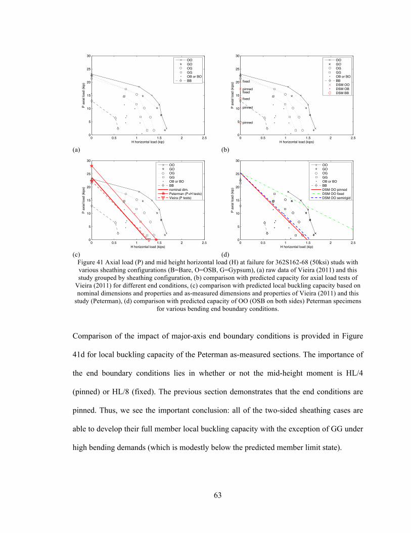
9.3 – Comparison of member limit states to tested capacity
The member limit state predictions of Table 11 are compared against the available test
data in Figure 41. The impact of sheathing on the strength follows clear trends (Figure
41a) with the exception of the OB and BO tests, which undergo significant torsion.
Although major-axis bending boundary conditions are shown to be essentially pinned in
the previous section, the illustration of the necessity of assuming fixed end conditions
under axial load is provided in Figure 41b. Weak-axis bending and torsion are
sufficiently restricted to create fixed end conditions even for specimens without sheathing.
Although the test data of Table 9 and Figure 41a provides all the data together as they are
nominally for the same 362S162-68 (50 ksi) stud the two test programs used different
batches of studs. The results, as depicted in Figure 41c, show that while the specimens
used for axial tests (Viera) are essentially identical to the nominal section, the specimens
used in the testing reported herein (Peterman) are markedly stronger. Care must be taken
when comparing predictions to the available data. The as-measured dimensions and
properties of the Peterman specimens are used for subsequent analysis.
63
(a) (b)
(c) (d)
Figure 41 Axial load (P) and mid height horizontal load (H) at failure for 362S162-68 (50ksi) studs with various sheathing configurations (B=Bare, O=OSB, G=Gypsum), (a) raw data of Vieira (2011) and this study grouped by sheathing configuration, (b) comparison with predicted capacity for axial load tests of
Vieira (2011) for different end conditions, (c) comparison with predicted local buckling capacity based on nominal dimensions and properties and as-measured dimensions and properties of Vieira (2011) and this
study (Peterman), (d) comparison with predicted capacity of OO (OSB on both sides) Peterman specimens for various bending end boundary conditions.
Comparison of the impact of major-axis end boundary conditions is provided in Figure
41d for local buckling capacity of the Peterman as-measured sections. The importance of
the end boundary conditions lies in whether or not the mid-height moment is HL/4
(pinned) or HL/8 (fixed). The previous section demonstrates that the end conditions are
pinned. Thus, we see the important conclusion: all of the two-sided sheathing cases are
able to develop their full member local buckling capacity with the exception of GG under
high bending demands (which is modestly below the predicted member limit state).
0 0.5 1 1.5 2 2.50
5
10
15
20
25
30
H horizontal load (kip)
P ax
ial lo
ad (k
ip)
OOGOOGGGOB or BOBB
0 0.5 1 1.5 2 2.50
5
10
15
20
25
30
pinned
fixed
pinned
fixed
pinned
fixed
H horizontal load (kips)
P ax
ial lo
ad (k
ips)
OOGOOGGGOB or BOBBDSM OODSM OBDSM BB
0 0.5 1 1.5 2 2.50
5
10
15
20
25
30
H horizontal load (kips)
P ax
ial lo
ad (k
ips)
OOGOOGGGOB or BOBBnominal dim.Peterman (P+H tests)Vieira (P tests)
0 0.5 1 1.5 2 2.50
5
10
15
20
25
30
H horizontal load (kip)
P ax
ial lo
ad (k
ip)
OOGOOGGGOB or BOBBDSM OO pinnedDSM OO fixedDSM OO semirigid
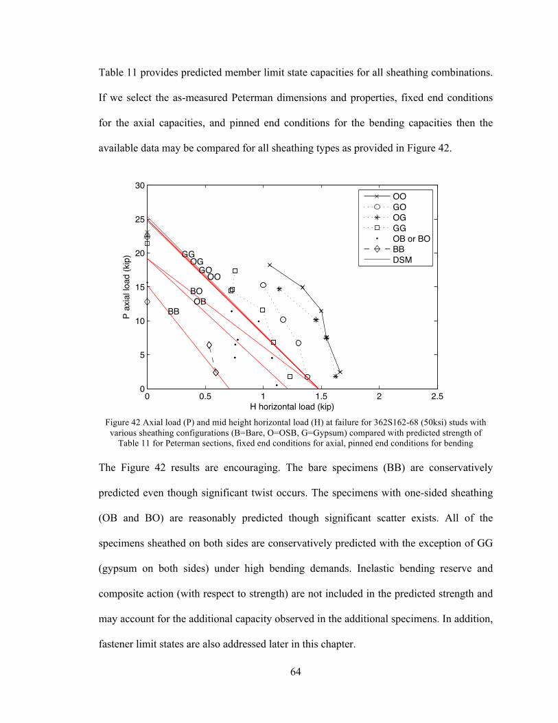
64
Table 11 provides predicted member limit state capacities for all sheathing combinations.
If we select the as-measured Peterman dimensions and properties, fixed end conditions
for the axial capacities, and pinned end conditions for the bending capacities then the
available data may be compared for all sheathing types as provided in Figure 42.
Figure 42 Axial load (P) and mid height horizontal load (H) at failure for 362S162-68 (50ksi) studs with
various sheathing configurations (B=Bare, O=OSB, G=Gypsum) compared with predicted strength of Table 11 for Peterman sections, fixed end conditions for axial, pinned end conditions for bending
The Figure 42 results are encouraging. The bare specimens (BB) are conservatively
predicted even though significant twist occurs. The specimens with one-sided sheathing
(OB and BO) are reasonably predicted though significant scatter exists. All of the
specimens sheathed on both sides are conservatively predicted with the exception of GG
(gypsum on both sides) under high bending demands. Inelastic bending reserve and
composite action (with respect to strength) are not included in the predicted strength and
may account for the additional capacity observed in the additional specimens. In addition,
fastener limit states are also addressed later in this chapter.
0 0.5 1 1.5 2 2.50
5
10
15
20
25
30
BBOB
BO
GGOG
GOOO
H horizontal load (kip)
P ax
ial lo
ad (k
ip)
OOGOOGGGOB or BOBBDSM

65
9.4 – Role of fastener stiffness in determining fastener demand
It is typical in design to assume that the fastener-sheathing system will supply full
torsional resistance to a sheathed member (stud), and thus the fasteners are designed to
carry the full torsional moment. However, in reality the torsional stiffness of the fastener-
sheathing system must be greater (significantly) than the member torsional stiffness, or
the torsion will be borne by the member (as well as the twist!).
The member and fastener-sheathing attachments relevant for resisting torsion are
provided in Figure 43. Here the springs are discrete (at each attachment location along
the length of the member) with values as provided in Figure 34.
Figure 43 Cross-section with springs simulating pull-through (k!) and bearing (kx)
resistance of sheathing on the two faces (1 and 2). To directly examine the impact of the fastener-sheathing stiffness the full system is
turned into a single equivalent rotational spring, k":
k! = k"1 + 1
4 kx1d2 + k"2 + 1
4 kx2d2
kx2
k!2"
kx1
k!1"
b/2
d/2
d/2

66
A simple beam element structural analysis model is created in MASTAN (Ziemian 2011).
The 362S162-68 (nominal dimensions) stud is modeled as warping continuous along the
length and warping free at its end. Rotational springs of stiffness k" are included in the
model every 12 in. A unit torque is applied at mid-height, and the resulting torsional
moment diagram and torsion in the springs are conceptually summarized in Figure 44
while Figure 45 provides the results directly from MASTAN.
Figure 44 Torsional stiffness analysis model depicting (a) basic model, (b) torsional moment diagram without springs, (c) torsional moment diagram and spring forces for typical fastener-sheathing spring
stiffness, (d) torsional moment diagram and spring force for infinitely stiff spring.
k!
k!
k!
k!
k!
k!
k!
Tapp
0.5Tapp
0.5Tapp
Tspr=Tapp Tspr=0.4Tapp
Tspr=0.3Tapp
Tspr=0.3Tapp
0.5Tapp
0.5Tapp
!"#$ !%#$ !&#$ !'#$
increasing k!"k!=0" k!=!"typ. k!"

67
Figure 45 Torsional moment diagram from MASTAN torsional stiffness analysis, note localization and
reduction of torsional demands in the member as torsional spring stiffness increases.
Noting that the member rotational stiffness (k$ member) is 3.2 kip-in./rad and that a bare
stud of 96 in. in height with a 1 kip-in. unit torque at mid-height rotates ($bare) 0.312 rad
(18 deg!) a parametric study varying the 12 in. o.c. discretely spaced rotational spring k$
from 0.01 kip-in./rad to 10,000 kip-in./rad is performed. The mid-height rotation and
torsion in the spring at mid-height are reported in Figure 46. The behavior at the limits is
consistent and understandable, but typical spring stiffness values lie in the middle. In this
intermediate range the fasteners do not see the full torsional demand at the midspan
fastener, but the result is the member twists – this is consistent with what was observed in
the testing herein.
k!=0"
!"#$!"#$
k!= 1"
!"%&$!"%&$
!"&'$
!"&'$
!"(($!"(($
!"!'$
!"!'$
!")'$!")'$
k!= 10" k!= 100"
*+,$ *-,$ *.,$ */,$

68
Figure 46 Torsional stiffness analysis depicting member rotation at mid-height and torsion in the mid-
height discrete spring as a function of rotational stiffness of the spring normalized by rotational stiffness of the member
It is concluded that a valid alternative to assuming that the fasteners must carry the full
torsional demand is to perform a torsional stiffness analysis as conducted here. The
impact of this model on the predicted capacities for fastener limit states is investigated in
the next section. Additional impacts of such an analysis are a need to examine or limit
member rotations, and the reality that direct torsional stresses are introduced into the
member.
10 4 10 2 100 102 1040
0.2
0.4
0.6
0.8
1
/ba
re m
idsp
an ro
tatio
n
k /k member
typical springrange
10 4 10 2 100 102 1040
0.2
0.4
0.6
0.8
1
T sprin
g/(Tap
p=1)
member rotationspring torsion

69
9.5 – Demands and Fastener Limit States
Stiffness (Figure 34, kx, k!) and capacity (Table 12, Ppt, Pbr) are known for the fastener-
sheathing systems (i.e., combinations of fasteners and sheathing) tested.
For one-sided sheathing, Figure 47, the only mechanism that can resist torsional demand
is the rotational restraint mechanism that includes bearing and pull-through. The torsional
moment on face “i” (where i is either 1 or 2) is
Pull-through related torsional resistance Tpti !( ) = k"i!
Tpti( )max = Ppti b / 2( ) = k!i"pti
For two-sided sheathing, Figure 48 and Figure 49, (where “i” refers to face 1 and 2), both
the pull-through related and bearing related mechanisms may exist, specifically:
Pull-through related torsional resistance Tpti !( ) = k"i!
Tpti( )max = Ppti b / 2( ) = k!i"pti
Bearing related torsional resistance Tbri !( ) = kxi d 2 / 4( )!
Tbri( )max = Pbri d / 2( ) = kxi d 2 / 4( )!bri
The total torsional resistance supplied by the fastener-sheathing may either be based on
first failure:
Torsional resistance at first failure ! f =min !pt1,!br1,!pt2,!br2( ) T1 = T (! f ) = Tpt1(! f )+Tbr1(! f )+Tpt2 (! f )+Tbr2 (! f )

70
Or instead may be based on fully ductile failure response in the fastener-sheathing system
and thus based on maximum strength
Torsional resistance, fully ductile maximum strength T2 = Tpt1( )max + Tbr1( )max + Tpt2( )max + Tbr2( )max
The basic values for face 1 and 2 are provided in Table 13.
Figure 47 Fastener-sheathing stiffness models for one-sided sheathing (a) one-sided sheathing on loaded
face, (b) rotational spring, modeling force couple from bearing into the board and pull-through at fastener, (c) sheathing on unloaded face, (d) rotational spring model similar to b.
Figure 48 Fastener-sheathing stiffness models for (a) two-sided sheathing, (b) model 1, standard model, including pull-through related (k!) and bearing resistance (kx) springs on both faces, (c) model 2, pull-
through related rotational spring on loaded face, bearing spring on unloaded face, (d) model 3, pull-through related and bearing springs on loaded face, bearing only spring on unloaded face.
k!2"
k!1"!"#$ !%#$ !&#$ !'#$
kx1
kx2
k!2"
k!1" kx1
k!2"
kx1
kx2
k!2"
!"#$ !%#$ !&#$ !'#$

71
Figure 49 Model 1, standard model, (a) springs, and (b) forces, including pull-through (Ppt) and bearing
(Pbr)
Table 13 Basic strength and stiffness of springs modeling fastener-sheathing system
For two-sided sheathing three models are considered for the development of the torsional
resistance of the fastener-sheathing system: model 1, Figure 47b, assumes that both
bearing and pull-through related mechanisms are engaged; model 2, Figure 47c, assumes
that pull-through related mechanisms govern for the unloaded face where the flange
twists away from the board and sheathing related mechanics govern for the flange which
twists toward the board; model 3, Figure 47b, assumes that bearing exists for both flanges,
but pull-through only for the loaded flange (face 2) which twists away from the board.
kx2
k!2"
kx1
k!1"
b/2
d/2
d/2
Pbr1
b/2
d/2
d/2
Pbr2 Ppt2
Ppt2
Ppt1 Ppt1
!"#$ !%#$
face 1: unloaded face/flange in test (flange twists toward board typ.) face 2: loaded face/flange in test (flange twists away from board typ.)Pbr1 kx1 Tbr1 qbr1 Ppt1 kf1 Tpt1 qpt1 Pbr2 kx2 Tbr2 qbr2 Ppt2 kf2 Tpt2 qpt2
sheathing (lbf) (kip/in.) (kip-in.) (rad) (lbf) (kip-in./rad) (kip-in.) (rad) (lbf) (kip/in.) (kip-in.) (rad) (lbf) (kip-in./rad) (kip-in.) (rad)BB - - - - - - - - - - - - - - - -OB - - - - 437 0.84 0.35 0.42 - - - - - - - -BO - - - - - - - - - - - - 437 0.84 0.35 0.42GG 86 2.43 0.16 0.02 40 0.85 0.03 0.04 86 2.43 0.16 0.02 40 0.85 0.03 0.04OG 578 5.52 1.05 0.06 437 0.84 0.35 0.42 86 2.43 0.16 0.02 40 0.85 0.03 0.04GO 86 2.43 0.16 0.02 40 0.85 0.03 0.04 578 5.52 1.05 0.06 437 0.84 0.35 0.42OO 578 5.52 1.05 0.06 437 0.84 0.35 0.42 578 5.52 1.05 0.06 437 0.84 0.35 0.42
d = 3.62 in., b = 1.62 in., e = 0.91 in.

72
For each model four predicted torsional capacities are investigated, e.g. for model 1:
pred. 1-1 fastener resists full torsional demand, failure at first mechanism, H1=T1/e
pred. 1-2 fastener resists full torsional demand, max fastener capacities, H2=T2/e
pred. 1-3 fastener demand from stiffness analysis, failure at first mechanism, H3=T1/Tspr/e
pred. 1-4 fastener demand from stiffness analysis, max fastener capacities, H4=T2/Tspr/e
Table 14 Detailed strength predictions for fastener limit state based failure for three models (see Figure 48)
Focusing on model 1, consider pred. 1-2 which is the closest to modern strength design
assumptions: i.e., torsional resistance is equal to the sum of the mechanisms, and it is
assumed that the full torsional demand must be resisted by the fastener. Figure 50a
provides the comparison to pred. 1-2, the results indicate that the OB, BO, and GG
sheathed conditions should fail around 0.4 kips horizontal force and the OG, GO, and OO
model 1:standard model, all springs engaged pred. 1-1 pred. 1-2 analysis (Tapp=1) pred. 1-3 pred. 1-4 test
kq qf T1=T(qf)T2=sum(T) q(T2) H1=T1/e q1 H2=T2/e q2 Tspr qmid H3=T1/Tspr/e q3 H4=T2/Tspr/e q4 H 1
sheathing (kip-in./rad) (rad) (kip-in.) (kip-in.) (rad) (kip) (deg) (kip) (deg) (kip-in.) (rad) (kip) (deg) (kip) (deg) (kip)BB - - - - - - - - - - 0.312 - - - - 0.59OB 0.84 0.421 0.35 0.35 0.421 0.389 24.14 0.389 24.14 0.14 0.173 2.711 24.41 2.711 24.41 1.120BO 0.84 0.421 0.35 0.35 0.421 0.389 24.14 0.389 24.14 0.14 0.173 2.711 24.41 2.711 24.41 1.080GG 17.62 0.020 0.34 0.38 0.038 0.379 1.12 0.413 2.18 0.40 0.026 0.941 1.30 1.027 1.42 1.230OG 27.73 0.020 0.54 1.59 0.421 0.596 1.12 1.745 24.14 0.45 0.020 1.320 1.37 3.865 4.02 1.380
GO 27.73 0.020 0.54 1.59 0.421 0.596 1.12 1.745 24.14 0.45 0.020 1.320 1.37 3.865 4.02 1.630OO 37.85 0.058 2.19 2.80 0.421 2.406 3.31 3.077 24.14 0.49 0.017 4.930 4.26 6.305 5.45 1.660
model 2: pull-through face 2, bearing face 1pred. 2-1 pred. 2-2 analysis (Tapp=1) pred. 2-3 pred. 2-4 test
kq qf T1=T(qf)T2=sum(T) q(T2) H1=T1/e q1 H2=T2/e q2 Tspr qmid H3=T1/Tspr/e q3 H3=T2/Tspr/e q4 H 1
sheathing (kip-in./rad) (rad) (kip-in.) (kip-in.) (rad) (kip) (deg) (kip) (deg) (kip-in.) (rad) (kip) (deg) (kip) (deg) (kip)BB - - - - - - - - - - 0.312 - - - - 0.59OB 0.84 0.421 0.35 0.35 0.421 0.389 24.14 0.389 24.14 0.14 0.173 2.711 24.41 2.711 24.41 1.120BO 0.84 0.421 0.35 0.35 0.421 0.389 24.14 0.389 24.14 0.14 0.173 2.711 24.41 2.711 24.41 1.080GG 8.81 0.020 0.17 0.19 0.038 0.189 1.12 0.207 2.18 0.34 0.042 0.562 1.22 0.614 1.34 1.230OG 18.93 0.038 0.72 1.08 0.058 0.793 2.18 1.185 3.31 0.41 0.025 1.935 2.55 2.892 3.81 1.380GO 8.80 0.020 0.17 0.51 0.421 0.189 1.12 0.560 24.14 0.34 0.042 0.556 1.22 1.647 3.61 1.630OO 18.92 0.058 1.09 1.40 0.421 1.203 3.31 1.539 24.14 0.41 0.025 2.935 3.87 3.754 4.95 1.660
model 3: pull-through face 2, bearing face 1 and 2pred. 3-1 pred. 3-2 analysis (Tapp=1) pred. 3-3 pred. 3-4 test
kq qf T1=T(qf)T2=sum(T) q(T2) H1=T1/e q1 H2=T2/e q2 Tspr qmid H3=T1/Tspr/e q3 H3=T2/Tspr/e q4 H 1
sheathing (kip-in./rad) (rad) (kip-in.) (kip-in.) (rad) (kip) (deg) (kip) (deg) (kip-in.) (rad) (kip) (deg) (kip) (deg) (kip)BB - - - - - - - - - - 0.312 - - - - 0.59OB 0.84 0.421 0.35 0.35 0.421 0.389 24.14 0.389 24.14 0.14 0.173 2.711 24.41 2.711 24.41 1.120BO 0.84 0.421 0.35 0.35 0.421 0.389 24.14 0.389 24.14 0.14 0.173 2.711 24.41 2.711 24.41 1.080GG 16.77 0.020 0.33 0.34 0.038 0.360 1.12 0.378 2.18 0.40 0.027 0.907 1.29 0.950 1.35 1.230OG 26.89 0.020 0.53 1.23 0.058 0.578 1.12 1.356 3.31 0.45 0.020 1.290 1.37 3.027 3.21 1.380GO 26.88 0.020 0.53 1.56 0.421 0.578 1.12 1.710 24.14 0.45 0.020 1.289 1.37 3.815 4.05 1.630OO 37.01 0.058 2.14 2.45 0.421 2.353 3.31 2.688 24.14 0.49 0.017 4.847 4.25 5.538 4.85 1.660
1. Maximum horizontal load observed in testing, generally for 10%Paxial, see Table of test results.
73
should not fail due to fasteners limit states, but rather yielding. The results are not
consistent with the test observations and if implemented would lead to excessively
conservative capacity predictions based on fastener limit states that do not occur. They do
not occur because the stiffness of the fastener-sheathing is not great enough to place all
the demand in the fasteners alone.
Model 1, pred. 1-3, would appear to be the most rational choice – the torsional capacity is
based on first failure in either pull-through or bearing for either face 1 or face 2 – and the
torsional demand is based on a stiffness analysis between the member torsional stiffness
and the supplied fastener-sheathing torsional stiffness. Figure 50b provides the results
compared with the test data. The one-sided sheathing cases (OB,BO) are not predicted to
fail by fastener failure, and indeed they did not, they failed by excessive torsion.
For pred. 1-3 the member with gypsum sheathed on both sides (GG) is predicted to fail at
H=0.94 kips – in the tests the member was able to sustain 1.23 kips. Although the
prediction is conservative it does correctly capture the fact that at high bending demands
fastener limit states not member limit states control for the GG case; further, the
prediction (and the use of the torsional stiffness analysis) is a significant improvement of
pred. 1-1 or 1-2 which leads to GG capacities near 0.4 kips.
For pred. 1-3 the two-sided sheathing cases with OSB: OG, GO, OO are not predicted to
be controlled by fastener limit states; instead member limit states are predicted to control.
The accuracy of this is somewhat difficult to judge in the tests, as the members yield in

74
bending the torsional member resistance decreases and eventually fastener limit states are
observed. It is postulated the fastener limit states occur after the member limit state, but
this is not proven by the available observations.
(a) (b)
Figure 50 P vs. H summary plot of Figure 42 augmented with fastener limit states (a) pred. 1-2 fastener
limit states based on maximum strength AND all torsion assumed to be carried in the fastener, (b) pred. 1-3
fastener limit state based on first failure (bearing or pull-through) and fastener demands based on torsional
stiffness analysis as depicted in the previous section.
Model 2 (Figure 48c), which presumes that pull-through controls the loaded face and
bearing on the unloaded face was the original hypothesis of the research team. This
mechanism appeared most consistent with what was observed in the testing, but the
predicted strength are not consistent with the tests. For example, GO is predicted to be
much weaker than OG the bearing mechanism on the unloaded face dominates the
torsional resistance and G (gypsum is weker). However, the tested capacities are the
opposite and GO is stronger than OG. This an other inconsistencies leads to the rejection
of this hypothesis.
0 0.5 1 1.5 2 2.50
5
10
15
20
25
30
BBOB
BO
GGOG
GOOO
OB/BO
GG
OG/GO
OO 3.1 kips(conn. limit)
H horizontal load (kip)
P ax
ial lo
ad (k
ip)
OOGOOGGGOB or BOBBDSMconn. limit
0 0.5 1 1.5 2 2.50
5
10
15
20
25
30
BBOB
BO
GGOG
GOOO
GG OG/GOOG/GO
OB/BO 2.7 kips (conn. limit)
OO 4.9 kips (conn. limit)
H horizontal load (kip)
P ax
ial lo
ad (k
ip)
OOGOOGGGOB or BOBBDSMconn. limit

75
Model 3 (Figure 48d), which presumes bearing mechanisms exist for both flanges, and
only pull-through on the loaded flange provides similar capacities to model 1. However,
the model requires knowing the “loaded flange” and making assumptions about the pull-
through mechanism that seem inconsistent. Ultimately it is concluded that model 3 holds
know advantages over model 1.
76
Chapter 10 – Future Work
Integrate axial fastener demand calculations coming from stability with bending fastener
demand calculations coming from torsion due to shear center issues. Examine inelastic
reserve capacity to determine if this explains discrepancy between predicted and tested
strengths. Examine composite bending strength to determine if this explains discrepancy
between predicted and tested strengths.
Perform testing or modeling on a section that is local or distortional buckling critical in
bending, i.e. thinner 6 or 8 in. deep studs – the current 362S162-68 section essentially
develops its yield moment, so it is limited in some respect. Perform detailed ABAQUS
analysis of the fastener forces to examine (a) the accuracy of the beam torsional stiffness
analysis employed herein, and (b) provide additional guidance on the exact nature of the
resistance developed. Perform full scale axial wall tests to confirm extensions to full scale
wall including how fastener forces add across a wall.
Change end boundary conditions to an explicit pin about major axis bending instead of
the functional pin that is resulting with current details. Investigate torsional beam
stiffness model for uniform load (torsion) instead of point load (torsion) to better reflect
typical conditions. Simplify the fastener strength check. Current approach is logical, but
too complicated for everyday use. Summarize the complete design method proposed
herein from fastener stiffness and stability analysis fastener-sheathing contribution, to
member strength and limit states as well as fastener limit states.

77
Chapter 11 – Conclusions
Testing and analysis is conducted on a 8 ft. high 362S162-68 (50 ksi) stud connected to
362T162-68 (50ksi) track with varying combinations of oriented strand board (O),
gypsum board (G) and bare/no sheathing (B) connected to the two flanges and subject to
axial load (P) and a directly applied horizontal load (H) to induce major-axis bending of
the stud (and torsion due to the shear center of the stud). The results demonstrate that
sheathing has a definitive and positive impact on the stability and strength of the stud.
One-sided sheathing cases (OB and BO) significantly increase the strength above no
sheathing (BB), but the applied horizontal load induces significant torsion and the stud is
essentially limited by serviceability/excessive twist. Two-sided sheathing cases (with one
exception) develop their full member capacity and show a clear progression in capacity
with two-sided gypsum board (GG) being the weakest, and the strength increasing with
the mixed cases from OG to GO up to the two-sided OSB (OO), which is the strongest.
Deformations at the stud-fastener-sheathing locations are a dominant visual portion of the
observed response as the sheathing attempts to stabilize the stud against torsion demand
(He) developed from the horizontal load H being applied by direct bearing and thus a
distance e away from the shear center. In the testing the descending branch of the strength
response typically initiates when pull-through of the center fastener through the sheathing
is observed; however, comparison against the member strength for all the two-sided
sheathing cases (excepting GG) shows that this fastener failure does not precipitate the
failure, but rather occurs after the specimen has developed its bending yield capacity (and
78
presumably is weakening, thus increasing demands to the fasteners). In the gypsum
sheathed case the pull-through failure occurs before the member reaches full yield. It is
further shown herein that none of the fastener-sheathing combinations utilized herein
completely restrict torsion in the stud – as a result accurately determining the fastener
demands to assess fastener limit states requires a torsional stiffness analysis. Such an
analysis is demonstrated herein, and it does properly capture the inadequacy of the
gypsum-sheathed case when compared against OSB or mixed OSB-gypsum sheathing.
The analysis provided herein provides a means to perform a detailed assessment of a CFS
stud wall under axial load and bending with differing sheathing configurations. One first
determines the stiffness and strength of the fastener-sheathing system that will be
providing resistance to the stud. This may be done by test (preferably) or using simplified
closed-formed solutions (previously developed, but conservative). Second, the member
stability in local, distortional, and global buckling must then be assessed. This may be
done by computational analysis (preferably) or using closed-form solutions (previously
developed, but involved). Third, the member stability analyses is used to assess the
member limit states using either effective width or Direct Strength Method approaches,
Direct Strength Method is demonstrated herein. Direct torsion was not considered in the
member limit state analyses performed herein, but is included in the fastener limit states.
Fourth, the fastener-sheathing capacities must be determined for pull-through and bearing
limit states. The authors were unable to find generally available methods or industry
reported values for these limit states and thus instead relied on our own direct testing
(previously conducted). Fifth, to determine the fastener demands one may assume all the
79
torsion must be carried by the fasteners or perform a torsional stiffness analysis to
determine the proportion carried by the member vs. that carried by the fastener-sheathing
combination (preferred). Finally, the minimum of the member and fastener limit states
controls the strength.
Cold-formed steel stud walls braced by sheathing and subjected to axial and bending
loads can provide the full member capacity (i.e. the local buckling limited strength) if
properly detailed. Additional work is needed to simply the design approach and develop
procedures for use in everyday design.

80
References
AISI, “Light Gage Cold-Formed Steel Design Manual.” American Iron and Steel Institute, 1962.
CFS, RSG Software, http://www.rsgsoftware.com/products.html
Fiorino, L., G. Della Corte, and R. Landolfo. (2007) “Experimental tests on typical screw connections for cold-formed steel housing.” Engineering Structures. 29(8): p. 1761-1773.
Li, Z., Schafer, B.W. (2010) “Buckling analysis of cold-formed steel members with general boundary conditions using CUFSM: conventional and constrained finite strip methods.” Proceedings of the 20th Int’l. Spec. Conf. on Cold-Formed Steel Structures, St. Louis, MO. November, 2010.
Miller, T. H. and T. Peköz, (1993) “Behavior of cold-formed wall stud-assemblies.” Journal of Structural Engineering, New York, N.Y., 119(2): p. 641-651.
Okasha, A.F., (2004) “Performance of Steel Frame/Wood Sheathing Screw Connections Subjected to Monotonic and Cyclic Loading.” MS Thesis submitted to McGill University.
Schafer, B. W., Vieira Jr., L. C. M., Sangree, R. H., Guan, Y. (2010) "Rotational Restraint and Distortional Buckling in Cold-Formed Steel Framing Systems." Revista Sul-Americana de Engenharia Estrutural (South American Journal of Structural Engineering), Special issue on cold-formed steel structures, 7 (1) 71-90.
Steel Stud Manufacturers Association (SSMA) (2010) Product Technical Information.
Vieira Jr., L. C. M., Schafer, B.W. “Lateral Stiffness and Strength of Sheathing Braced Cold-Formed Steel Stud Walls.” Elsevier, Engineering Structures. (Accepted 2011).
Vieira Jr., L. C. M., Shifferaw, Y., Schafer, B.W. (2011) “Experiments on Sheathed Cold-Formed Steel Studs in Compression.” Elsevier, Journal of Constructional Steel Research. 67 (10) 1554-1566 (doi:10.1016/j.jcsr.2011.03.029).
Related non-refereed conference paper: Shifferaw, Y., Vieira Jr., L.C.M., Schafer, B.W. (2010). “Compression testing of cold-formed steel columns with different sheathing configurations.” Proc. of the Structural Stability Research Council - Annual Stability Conference, Orlando, FL. 593-612.
Simaan, A. and T.B. Peköz, (1976) “Diaphragm Braced Members and Design of Wall Studs.” ASCE J Struct Div. 102(1): p. 77-92.
Winter, G. (1960) “Lateral Bracing of Beams and Columns.” Journal of the Structural Division.
Vieira Jr., L.C.M (2011). “Behavior and Design of Sheathed Cold-Formed Steel Stud Walls Under Compression." Doctoral Dissertation submitted to Johns Hopkins University.
Vieira Jr., L.C.M (2011). “Behavior and Design of Sheathed Cold-Formed Steel Stud Walls Under Compression." Doctoral Dissertation submitted to Johns Hopkins University.
Zeinoddini, V (2011). “Geometric Imperfections in Cold-Formed Steel Members.” Doctoral Dissertation submitted to Johns Hopkins University.

81
Appendices
Appendix A: Specimen reference (Shifferaw, et al., 2010)
abbrev. full reference name P(kips) P(kN) 1-BARE-BARE-7S6L-6 2-BARE-BARE-1S6L-6 3-BARE-BARE-1S4L-4 4-BARE-BARE-1S2L-2
5 (2') 5-BARE-BARE-1S2LT-2-T 19.77 87.95 6 (4') 6-BARE-BARE-2S4LT-4-T 19.03 84.63 7 (6') 7-BARE-BARE-2S6LT-6-T 13.59 60.46
8-OSB-OSB-3S6LTS-6-T-S 11-GYP-GYP-8S6LTSP-6-T-S
12 (6') 12-OSB-BARE-6S6LTSP-6-T-S-P 18.01 80.13 13 (6') 13-OSB-GYP-7S6LTSP-6-T-S-P 20.48 91.11 14 (4') 14-OSB-BARE-3S4LTSP-4-T-S-P 21.99 97.82 15 (4') 15-GYP-GYP-4S4LTSP-4-T-S-P 22.39 99.61 16 (4') 16-GYP-OSB-5S4LTSP-4-T-S-P 21.62 96.17 17 (4') 17-OSB-OSB-6S4LTSP-4-T-S-P 22.25 98.99 18 (2') 18-OSB-BARE-4S2LTSP-2-T-S-P 21.45 95.41 19 (2') 19-GYP-GYP-3S2LTSP-2-T-S-P 21.74 96.71 20 (2') 20-OSB-GYP-5S2LTSP-2-T-S-P 21.99 97.82 21 (2') 21-OSB-OSB-6S2LTSP-2-T-S-P 22.84 101.59 22 (8') 22-BARE-BARE-61S8LTP-8-T-P 12.84 57.11 23 (8') 23-OSB-BARE-62S8LTSP-8-T-S-P 15.64 69.57 24 (8') 24-OSB-GYP-63S8LTSP-8-T-S-P 22.45 99.86 25 (8') 25-GYP-GYP-64S8LTSP-8-T-S-P 21.37 95.05 26 (8') 26-OSB-OSB-65S8LTSP-8-T-S-P 23.09 102.7
82
Appendix B: Tensile Results
Coated Specimens
0 0.05 0.1 0.15 0.2 0.250
10
20
30
40
50
60
70
80
90
100
Engineering Strain,(in./in.)
Axia
l Ten
sile
Stre
ss (k
si)
cfs12.txt
YIELD STRESS (0.2% offset)=60.7 ksi
0 0.05 0.1 0.15 0.2 0.250
10
20
30
40
50
60
70
80
90
100
Engineering Strain (in./in.)
Axia
l Ten
sile
Stre
ss (k
si)
cfs21.txt
YIELD STRESS (Autographic Method)=59.5 ksi
0 0.05 0.1 0.15 0.2 0.250
10
20
30
40
50
60
70
80
90
100
Engineering Strain (in./in.)
Axia
l Ten
sile
Stre
ss (k
si)
cfs31.txt
YIELD STRESS (Autographic Method)=59.8 ksi
0 0.05 0.1 0.15 0.2 0.250
10
20
30
40
50
60
70
80
90
100
Engineering Strain (in./in.)
Axia
l Ten
sile
Stre
ss (k
si)
cfs33.txt
YIELD STRESS (Autographic Method)=59.9 ksi

83
Uncoated Specimens
0 0.05 0.1 0.15 0.2 0.250
10
20
30
40
50
60
70
80
90
100
Engineering Strain (in./in.)
Axia
l Ten
sile
Stre
ss (k
si)
cfs13.txt
YIELD STRESS (Autographic Method)=60.7 ksi
0 0.05 0.1 0.15 0.2 0.250
10
20
30
40
50
60
70
80
90
100
Engineering Strain (in./in.)
Axia
l Ten
sile
Stre
ss (k
si)
cfs22.txt
YIELD STRESS (Autographic Method)=59.2 ksi
0 0.05 0.1 0.15 0.2 0.250
10
20
30
40
50
60
70
80
90
100
Engineering Strain (in./in.)
Axia
l Ten
sile
Stre
ss (k
si)
cfs23.txt
YIELD STRESS (Autographic Method)=59.5 ksi
0 0.05 0.1 0.15 0.2 0.250
10
20
30
40
50
60
70
80
90
100
Engineering Strain (in./in.)
Axia
l Ten
sile
Stre
ss (k
si)
cfs32.txt
YIELD STRESS (Autographic Method)=60.2 ksi

84
Appendix C: Tensile Specimen Measurements
Coated Specimens
specimen # s1c2 s2c1 s3c1 s3c3 dimension thick. (in) width (in) thick. (in) width (in) thick. (in) width (in) thick. (in) width (in)
1 0.076 0.497 0.0729 0.497 0.0735 0.4945 0.0729 0.495
2 0.077 0.4965 0.0736 0.497 0.0731 0.4945 0.073 0.4965
3 0.0735 0.497 0.0724 0.496 0.0729 0.4945 0.0731 0.495
4 0.073 0.496 0.0732 0.4965 0.0729 0.4955 0.0729 0.496
5 0.073 0.495 0.0727 0.496 0.073 0.4955 0.0726 0.4945
mean 0.0745 0.4963 0.07296 0.4965 0.07308 0.4949 0.0729 0.4954
Uncoated Specimens
specimen # s1c3 s2c2 s2c3 s3c2
dimension thick. (in) width (in) thick. (in) width (in) thick. (in) width (in) thick. (in) width (in)
1 0.0715 0.494 0.0715 0.4925 0.0717 0.4945 0.0715 0.4965
2 0.0716 0.494 0.0715 0.4925 0.0716 0.4965 0.0716 0.4955
3 0.0715 0.4935 0.0716 0.4925 0.0716 0.495 0.0716 0.4955
4 0.0715 0.494 0.0716 0.493 0.0716 0.4955 0.0716 0.4955
5 0.0715 0.494 0.0717 0.493 0.0716 0.495 0.0714 0.4955
mean 0.07152 0.4939 0.07158 0.4927 0.07162 0.4953 0.07154 0.4957

85
Appendix D: Complete Imperfection Measurements
Stud # L (in) d1/t d2/t G1/L G2/L G3/L
(deg/ft) 1 0.03 0.48 0.83 750 1181 0.11 2 0.01 0.22 0.95 834 701 0.11 3 0.02 0.28 0.81 887 1386 0.05 4 0.07 1.05 0.67 1010 5864 0.06 5 0.03 0.40 0.78 975 1309 0.05 6 0.04 0.54 0.80 1307 1972 0.31 7 0.04 0.60 1.27 1913 2488 0.23 8 0.02 0.35 0.66 1496 1031 0.08 9 0.02 0.36 0.98 1334 2011 0.16
10 0.03 0.49 0.82 909 1520 0.15 11 0.03 0.45 1.76 338 1254 0.12 12 0.04 0.58 0.92 1664 960 0.13 13 0.02 0.36 1.01 1308 1508 0.13 14 0.04 0.55 0.94 1415 1724 0.16 15 0.02 0.28 0.88 1426 1043 0.05 16 0.03 0.47 0.90 1900 803 0.17 17 0.02 0.36 1.01 2283 926 0.15 18 0.04 0.62 0.79 1023 1330 0.07 19 0.03 0.49 0.75 1341 1440 0.04 20 0.04 0.56 0.67 930 1727 0.12 21 0.03 0.40 0.97 1320 2247 0.09 22 0.02 0.36 0.70 953 1314 0.05 23 0.03 0.39 1.11 1017 1276 0.04 24 0.03 0.47 0.76 1143 1366 0.06 25 0.06 0.81 0.96 1273 963 0.13 26 0.02 0.36 0.84 1096 1214 0.11 27 0.03 0.46 0.87 920 1837 0.19 28 0.04 0.54 0.76 971 1970 0.13 29 0.04 0.56 0.91 851 1388 0.11 30 0.05 0.68 0.72 1669 1381 0.06
MEAN 0.48 0.89 1209 1571 0.11
ST. DEV 0.17 0.21 402 915 0.06
86
Appendix E: Complete Cross-Section Measurements
All measurements are in inches.
Stud h B-A B-B D-A D-B t Rhb-B Rdb-B Rhb-A Rdb-A !hb-B !db-B !hb-A !db-A39 3.685 1.683 1.682 0.590 0.551 0.082 1/4 15/64 1/4 1/4 87.8 87.4 88.5 87.2
3.685 1.711 1.696 0.581 0.559 0.077 1/4 15/64 1/4 1/4 87.5 85.9 88.7 87.03.683 1.700 1.674 0.591 0.513 0.075 1/4 15/64 1/4 1/4 86.4 86.8 88.8 87.3
32 3.684 1.680 1.691 0.570 0.556 0.078 11/32 1/4 9/32 23/64 85.8 88.1 88.5 88.73.691 1.688 1.703 0.521 0.565 0.077 11/32 15/64 19/64 23/64 86.2 87.4 88.4 89.53.691 1.686 1.709 0.550 0.556 0.078 23/64 1/4 9/32 23/64 86.8 87.8 88.9 89.1
35 3.680 1.678 1.698 0.542 0.559 0.081 23/64 11/32 5/16 15/64 87.2 82.8 85.9 90.03.678 1.685 1.703 0.549 0.575 0.077 23/64 11/32 11/32 15/64 88.7 88.8 86.8 89.83.677 1.678 1.701 0.547 0.559 0.077 23/64 11/32 5/16 15/64 87.5 87.0 85.4 89.5
38 3.678 1.709 1.689 0.586 0.566 0.077 23/64 17/64 23/64 5/16 85.4 86.1 87.1 79.33.681 1.709 1.689 0.575 0.564 0.078 23/64 17/64 23/64 5/16 85.0 85.6 88.3 79.03.679 1.709 1.685 0.593 0.561 0.078 23/64 17/64 23/64 5/16 89.8 86.9 88.2 82.6
37 3.672 1.688 1.702 0.581 0.504 0.077 3/8 5/16 11/32 17/64 92.0 82.1 85.5 90.03.677 1.673 1.703 0.553 0.554 0.077 3/8 5/16 23/64 17/64 91.5 78.3 87.5 87.73.678 1.676 1.702 0.585 0.567 0.076 3/8 5/16 11/32 17/64 91.3 78.1 88.0 90.2
36 3.676 1.666 1.718 0.510 0.587 0.077 3/8 5/16 23/64 17/64 91.7 79.8 88.5 87.23.673 1.674 1.715 0.690 0.576 0.078 3/8 5/16 23/64 17/64 91.6 78.7 86.4 88.33.675 1.671 1.709 0.558 0.591 0.076 23/64 11/32 23/64 17/64 91.3 78.9 86.3 87.3
9 3.675 1.688 1.706 0.566 0.551 0.077 23/64 11/32 11/32 17/64 92.1 89.3 93.2 87.13.680 1.685 1.700 0.621 0.569 0.076 23/64 11/32 11/32 17/64 88.9 86.5 94.0 87.23.673 1.683 1.701 0.587 0.563 0.077 11/32 17/64 11/32 17/64 91.3 86.7 90.4 89.4
33 3.671 1.701 1.674 0.570 0.577 0.077 11/32 17/64 25/64 11/32 93.2 91.2 87.6 81.53.677 1.711 1.689 0.614 0.602 0.078 11/32 17/64 13/16 23/64 93.9 91.7 88.4 85.43.676 1.704 1.681 0.588 0.583 0.077 11/32 17/64 13/16 23/64 92.5 91.0 87.9 82.4
34 3.671 1.717 1.689 0.571 0.596 0.078 11/32 17/64 11/32 11/32 87.3 88.5 88.2 84.36.675 1.704 1.687 0.593 0.601 0.078 11/32 17/64 11/32 11/32 86.4 84.6 88.3 86.33.672 1.707 1.691 0.584 0.599 0.078 11/32 17/64 11/32 11/32 86.9 85.7 87.9 85.0
31 3.679 1.718 1.682 0.578 0.568 0.077 23/64 19/64 3/8 11/32 86.1 88.2 88.7 73.43.681 1.717 1.697 0.571 0.581 0.078 23/64 19/64 3/8 21/64 84.3 84.7 88.0 73.73.680 1.719 1.689 0.573 0.575 0.078 23/64 19/64 3/8 11/32 84.8 85.6 88.5 73.5
30 3.685 1.696 1.690 0.573 0.591 0.078 11/32 17/64 11/32 11/32 86.6 88.8 89.8 84.43.686 1.699 1.686 0.585 0.586 0.078 11/32 17/64 25/64 11/32 89.8 89.4 88.6 82.43.685 1.697 1.695 0.579 0.581 0.078 11/32 17/64 11/32 11/32 88.7 89.0 88.4 83.3
29 3.683 1.702 1.682 0.584 0.560 0.077 23/64 17/64 23/64 23/64 88.7 86.2 89.7 78.23.682 1.707 1.677 0.589 0.593 0.077 23/64 17/64 11/32 23/64 88.9 86.5 89.6 76.13.683 1.720 1.686 0.578 0.595 0.079 23/64 17/64 11/32 23/64 88.5 86.3 89.9 77.1
19 3.683 1.706 1.697 0.563 0.556 0.078 11/32 17/64 23/64 5/16 86.7 88.4 87.8 77.73.682 1.713 1.697 0.554 0.596 0.078 11/32 17/64 23/64 5/16 88.0 86.1 88.0 80.13.684 1.710 1.698 0.550 0.576 0.078 11/32 17/64 23/64 5/16 87.3 87.2 87.6 78.4
20 3.678 1.700 1.678 0.537 0.553 0.077 23/64 17/64 23/64 11/32 88.3 90.0 88.8 79.53.679 1.702 1.675 0.536 0.576 0.077 23/64 17/64 23/64 11/32 87.7 87.7 89.7 82.13.675 1.699 1.687 0.541 0.567 0.078 23/64 17/64 23/64 11/32 88.7 88.2 89.3 81.4
24 3.678 1.716 1.696 0.575 0.568 0.078 11/32 17/64 11/32 11/32 56.5 84.3 89.0 80.53.679 1.705 1.687 0.558 0.561 0.078 11/32 17/64 11/32 11/32 87.2 87.7 81.0 79.83.677 1.704 1.686 0.537 0.591 0.078 11/32 17/64 11/32 11/32 86.8 85.4 88.3 79.6
21 3.677 1.708 1.684 0.553 0.539 0.079 23/64 17/64 23/64 5/16 89.6 89.7 89.1 82.53.678 1.704 1.674 0.543 0.572 0.078 23/64 17/64 11/32 5/16 88.9 82.2 89.5 81.63.675 1.710 1.678 0.561 0.533 0.078 23/64 17/64 11/32 5/16 89.1 84.3 89.4 81.8
26 3.683 1.704 1.682 0.582 0.582 0.078 23/64 17/64 5/16 3/8 88.1 87.3 88.8 81.73.681 1.705 1.683 0.558 0.576 0.078 23/64 17/64 5/16 3/8 87.1 86.5 89.6 83.23.680 1.701 1.682 0.562 0.579 0.078 23/64 17/64 11/32 3/8 87.6 86.9 89.1 82.4
27 3.683 1.646 1.707 0.562 0.542 0.074 25/64 11/32 11/32 17/64 89.8 85.3 89.2 88.73.684 1.688 1.715 0.551 0.571 0.074 25/64 11/32 11/32 17/64 88.3 82.9 89.3 88.33.685 1.682 1.713 0.550 0.563 0.076 25/64 11/32 5/16 17/64 89.2 83.7 89.9 88.4
28 3.688 1.681 1.713 0.555 0.533 0.078 11/32 5/16 5/16 17/64 89.0 80.1 87.1 86.53.683 1.682 1.710 0.587 0.544 0.078 11/32 5/16 5/16 17/64 89.9 82.1 86.9 87.63.685 1.682 1.715 5.610 0.538 0.078 11/32 5/16 23/64 17/64 89.7 80.9 87.8 86.9
25 3.675 1.695 1.675 0.561 0.591 0.077 23/64 17/64 23/64 21/64 86.6 86.0 87.9 79.53.676 1.700 1.679 0.582 0.580 0.078 23/64 17/64 23/64 21/64 87.0 85.4 88.5 81.03.368 1.701 1.678 5.730 0.588 0.078 23/64 17/64 11/32 21/64 87.1 85.6 88.1 80.7
23 3.720 1.707 1.661 0.583 0.500 0.078 21/64 17/64 11/32 5/16 86.3 86.5 89.8 77.73.726 1.720 1.682 0.554 0.506 0.078 21/64 17/64 11/32 5/16 85.4 89.9 89.7 78.03.721 1.713 1.682 0.568 0.504 0.078 21/64 17/64 11/32 5/16 87.0 88.1 89.9 78.7
22 3.722 1.707 1.666 0.546 0.510 0.078 11/32 17/64 11/32 21/64 86.2 80.3 89.8 83.33.725 1.718 1.685 0.582 0.521 0.078 11/32 17/64 11/32 21/64 85.3 89.1 89.4 77.63.723 1.710 1.679 0.563 0.530 0.078 11/32 17/64 11/32 21/64 85.8 85.4 89.6 80.7
16 3.683 1.709 1.674 0.562 0.535 0.077 23/64 17/64 23/64 19/64 86.1 74.0 89.4 87.63.684 1.712 1.678 0.576 0.551 0.078 23/64 17/64 23/64 19/64 89.8 78.8 88.8 87.43.683 1.711 1.672 0.575 0.547 0.078 23/64 17/64 23/64 19/64 89.9 82.4 89.4 88.1
11 3.677 1.707 1.673 0.597 0.561 0.077 23/64 17/64 11/32 5/16 87.7 87.4 87.0 82.43.679 1.711 1.677 0.584 0.568 0.078 23/64 17/64 11/32 5/16 87.4 86.2 89.5 77.13.667 1.709 1.678 0.590 0.563 0.078 23/64 17/64 11/32 5/16 87.9 86.8 88.1 80.3
10 3.689 1.710 1.683 0.545 0.618 0.078 23/64 17/64 23/64 5/16 88.4 86.4 89.9 81.43.666 1.714 1.686 0.559 0.603 0.078 23/64 17/64 25/64 5/16 87.5 85.6 88.5 81.13.675 1.711 1.685 0.551 0.614 0.078 23/64 17/64 25/64 5/16 88.1 85.9 87.9 80.5
18 3.683 1.683 1.698 0.553 0.565 0.078 3/8 11/32 11/32 17/64 89.0 80.5 87.1 82.53.679 1.682 1.705 0.588 0.560 0.078 3/8 11/32 11/32 17/64 89.2 80.0 88.0 88.23.681 1.688 1.699 0.574 0.563 0.078 3/8 11/32 11/32 17/64 88.9 79.4 87.4 85.4

87
16 3.683 1.709 1.674 0.562 0.535 0.077 23/64 17/64 23/64 19/64 86.1 74.0 89.4 87.63.684 1.712 1.678 0.576 0.551 0.078 23/64 17/64 23/64 19/64 89.8 78.8 88.8 87.43.683 1.711 1.672 0.575 0.547 0.078 23/64 17/64 23/64 19/64 89.9 82.4 89.4 88.1
11 3.677 1.707 1.673 0.597 0.561 0.077 23/64 17/64 11/32 5/16 87.7 87.4 87.0 82.43.679 1.711 1.677 0.584 0.568 0.078 23/64 17/64 11/32 5/16 87.4 86.2 89.5 77.13.667 1.709 1.678 0.590 0.563 0.078 23/64 17/64 11/32 5/16 87.9 86.8 88.1 80.3
10 3.689 1.710 1.683 0.545 0.618 0.078 23/64 17/64 23/64 5/16 88.4 86.4 89.9 81.43.666 1.714 1.686 0.559 0.603 0.078 23/64 17/64 25/64 5/16 87.5 85.6 88.5 81.13.675 1.711 1.685 0.551 0.614 0.078 23/64 17/64 25/64 5/16 88.1 85.9 87.9 80.5
18 3.683 1.683 1.698 0.553 0.565 0.078 3/8 11/32 11/32 17/64 89.0 80.5 87.1 82.53.679 1.682 1.705 0.588 0.560 0.078 3/8 11/32 11/32 17/64 89.2 80.0 88.0 88.23.681 1.688 1.699 0.574 0.563 0.078 3/8 11/32 11/32 17/64 88.9 79.4 87.4 85.4
15 3.683 1.703 1.684 0.551 0.570 0.078 23/64 17/64 3/8 11/32 89.8 88.8 88.2 77.33.682 1.706 1.677 0.592 0.573 0.078 23/64 17/64 3/8 11/32 86.6 89.4 89.3 72.43.681 1.708 1.680 0.584 0.574 0.078 23/64 17/64 3/8 11/32 87.4 89.1 88.7 75.3
14 3.719 1.710 1.660 0.533 0.545 0.077 21/64 17/64 11/32 11/32 85.4 84.8 89.9 78.13.714 1.708 1.680 0.582 0.522 0.078 21/64 17/64 11/32 11/32 85.8 87.1 89.7 76.83.720 1.711 1.675 0.551 0.531 0.078 21/64 17/64 11/32 11/32 86.1 85.4 89.8 77.4
13 3.680 1.682 1.704 0.535 0.565 0.079 25/64 21/64 11/32 17/64 89.8 85.7 86.7 88.73.675 1.685 1.709 0.546 0.555 0.078 25/64 21/64 11/32 17/64 89.7 80.7 88.5 87.73.677 1.688 1.713 0.544 0.541 0.079 25/64 21/64 11/32 17/64 89.9 83.2 89.1 87.4
12 3.681 1.680 1.700 0.549 0.591 0.078 23/64 11/32 21/64 17/64 89.1 85.8 86.5 87.63.681 1.691 1.719 0.553 0.507 0.078 23/64 11/32 21/64 17/64 89.9 78.7 89.3 87.53.680 1.674 1.720 0.585 0.575 0.078 23/64 11/32 21/64 17/64 89.5 83.4 88.4 87.3
7 3.719 1.702 1.682 0.543 0.554 0.077 21/64 17/64 23/64 5/16 88.8 78.2 89.5 80.13.715 1.709 1.677 0.515 0.521 0.078 21/64 17/64 23/64 5/16 89.3 75.8 90.0 77.53.711 1.704 1.679 0.534 0.538 0.078 21/64 17/64 23/64 5/16 89.8 76.4 89.9 78.9
8 3.679 1.688 1.706 0.548 0.564 0.078 11/32 5/16 21/64 17/64 88.8 79.3 87.6 87.93.685 1.680 1.704 0.567 0.570 0.078 11/32 5/16 21/64 17/64 89.3 75.2 87.0 84.73.683 1.691 1.707 0.575 0.571 0.078 11/32 5/16 21/64 17/64 88.4 77.7 87.1 84.1
6 3.681 1.715 1.684 0.562 0.541 0.077 23/64 17/64 23/64 11/32 85.6 84.3 89.0 79.83.682 1.713 1.685 0.565 0.562 0.077 23/64 17/64 23/64 11/32 86.3 88.7 80.3 79.73.681 1.714 1.689 0.564 0.554 0.077 23/64 17/64 23/64 11/32 87.1 86.4 85.4 79.1
5 3.682 1.686 1.705 0.585 0.521 0.078 11/32 23/64 17/64 5/16 89.7 89.3 80.5 79./3.686 1.681 1.709 0.564 0.546 0.078 11/32 23/64 17/64 5/16 87.7 88.4 81.7 77.73.384 1.687 1.710 0.571 0.533 0.078 11/32 23/64 17/64 5/16 88.0 88.9 81.1 78.4
4 3.679 1.704 1.684 0.573 0.516 0.077 11/32 25/64 5/16 17/64 89.7 86.6 78.1 86.53.681 1.710 1.920 0.591 0.512 0.077 11/32 25/64 5/16 17/64 89.3 87.3 79.8 84.83.600 1.709 1.688 0.584 0.523 0.780 11/32 25/64 5/16 17/64 89.4 87.1 78.4 85.4
3 3.688 1.708 1.683 0.571 0.549 0.079 23/64 11/32 11/32 17/64 89.8 88.0 76.3 89.13.687 1.714 1.676 0.556 0.561 0.078 23/64 11/32 11/32 17/64 89.9 88.3 74.1 89.63.690 1.722 1.679 0.562 0.555 0.078 23/64 11/32 11/32 17/64 89.7 88.4 75.2 89.4
2 3.684 1.699 1.678 0.573 0.552 0.077 23/64 23/64 11/32 17/64 86.2 87.7 78.2 87.73.684 1.711 1.690 0.563 0.568 0.077 23/64 23/64 11/32 17/64 89.2 87.6 73.5 84.13.683 1.704 1.684 0.568 0.566 0.078 23/64 23/64 11/32 17/64 88.7 87.8 75.7 85.7
1 3.683 1.688 1.704 0.533 0.572 0.077 23/64 11/32 17/64 11/32 86.5 88.7 89.7 79.53.684 1.684 1.708 0.536 0.587 0.078 23/64 11/32 17/64 11/32 89.4 89.9 87.3 71.83.380 1.680 1.707 0.539 0.580 0.078 23/64 11/32 17/64 11/32 88.2 89.4 88.1 76.3h B-A B-B D-A D-B t Rhb-B Rdb-B Rhb-A Rdb-A !hb-B !db-B !hb-A !db-A
mean 3.702 1.699 1.693 0.656 0.560 0.084 0.352 0.294 0.347 0.307 88.038 85.356 87.275 83.005
88
Appendix F: Temperature and Humidity Readings in JHU Laboratory

89
Appendix G: Addendum Test with 2 in. fastener spacing
An OO column (S31-OO*) with 2 inch fastener spacing was constructed as tested. As
anticipated, the stud experienced local buckling at mid-height. The fasteners withstood
the applied load easily—no damage was observed (Figure 51). Plotted on the P-M space,
this test also demonstrates that with greater fastener resistance, the stud can develop
significantly greater horizontal load capacity (approximately 2.2kips at 10%P loading).
(a). During test (b). Detail of local failure at mid-height
Figure 51: S31-OO* (2 inch fastener spacing)

90
Appendix H: Complete Specimen Response Summaries
S01 OOat P=7.57kipHmax=1.55kip
direct=0.061 in.
mid=1.554 in.
board=1.442 deg
x 10 at Hmax0 0.5 1 1.5
0
5
10
15
20
25
H horizontal load (kip)
P ax
ial l
oad
(kip
)
at P=7.57kip Hmax=1.55kip in.
S01 OO
0 0.1 0.2 0.30
5
10
15
20
25
axial disp. (in.)
P ax
ial l
oad
(kip
)
direct=0.061
direct
machine
0 0.5 1 1.5 20
0.5
1
1.5
2
mid side disp. (in.)
H h
oriz
. loa
d (k
ip)
mid=1.554
0 0.5 1 1.50
0.5
1
1.5
2
twist (deg)
H h
oriz
. loa
d (k
ip)
board=1.442
stud
board
15 10 5 0x 10 3
0
0.5
1
1.5
2
local (in.)
H h
oriz
. loa
d (k
ip)
middlebottom

91
S05 OGat P=6.71kipHmax=1.30kip
direct=0.055 in.
mid=1.376 in.
board= 0.213 deg
x 10 at Hmax0 0.5 1
0
5
10
15
20
25
H horizontal load (kip)
P ax
ial l
oad
(kip
)
at P=6.71kip Hmax=1.30kip in.
S05 OG
0 0.1 0.2 0.30
5
10
15
20
25
axial disp. (in.)
P ax
ial l
oad
(kip
)
direct=0.055
direct
machine
0 0.5 1 1.50
0.5
1
1.5
2
mid side disp. (in.)
H h
oriz
. loa
d (k
ip)
mid=1.376
0.2 0 0.2 0.4 0.60
0.5
1
1.5
2
twist (deg)
H h
oriz
. loa
d (k
ip)
board= 0.213
stud
board
10 5 0x 10 3
0
0.5
1
1.5
2
local (in.)
H h
oriz
. loa
d (k
ip)
middlebottom

92
S06 OBat P=0.50kip
Hmax=1.12kip
direct=0.026 in.
mid=1.982 in.
board=0.001 deg
x 10 at Hmax0 0.5 1
0
5
10
15
20
25
H horizontal load (kip)
P a
xial
load
(kip
)
at P=0.50kip Hmax=1.12kip in.
S06 OB
0 0.05 0.10
5
10
15
20
25
axial disp. (in.)
P a
xial
load
(kip
)
direct=0.026
direct
machine
0 0.5 1 1.5 20
0.5
1
1.5
2
mid side disp. (in.)
H h
oriz
. loa
d (k
ip)
mid=1.982
0 1 2 3 40
0.5
1
1.5
2
twist (deg)
H h
oriz
. loa
d (k
ip)
board=0.001
stud
board
6 4 2 0
x 10 3
0
0.5
1
1.5
2
local (in.)
H h
oriz
. loa
d (k
ip)
middlebottom

93
S07 OGat P=1.73kip
Hmax=1.38kip
direct=0.029 in.
mid=1.841 in.
board= 0.132 deg
x 10 at Hmax0 0.5 1
0
5
10
15
20
25
H horizontal load (kip)
P a
xial
load
(kip
)
at P=1.73kip Hmax=1.38kip in.
S07 OG
0 0.05 0.10
5
10
15
20
25
axial disp. (in.)
P a
xial
load
(kip
)
direct=0.029
direct
machine
0 0.5 1 1.5 20
0.5
1
1.5
2
mid side disp. (in.)
H h
oriz
. loa
d (k
ip)
mid=1.841
0 1 20
0.5
1
1.5
2
twist (deg)
H h
oriz
. loa
d (k
ip)
board= 0.132
stud
board
0 0.01 0.02 0.03 0.040
0.5
1
1.5
2
local (in.)
H h
oriz
. loa
d (k
ip)
middlebottom

94
S08 GOat P=10.16kip
Hmax=1.46kip
direct=0.062 in.
mid=1.387 in.
board=0.631 deg
x 10 at Hmax0 0.5 1 1.5
0
5
10
15
20
25
H horizontal load (kip)
P a
xial
load
(kip
)
at P=10.16kip Hmax=1.46kip in.
S08 GO
0 0.1 0.2 0.30
5
10
15
20
25
axial disp. (in.)
P a
xial
load
(kip
)
direct=0.062
direct
machine
0 0.5 1 1.50
0.5
1
1.5
2
mid side disp. (in.)
H h
oriz
. loa
d (k
ip)
mid=1.387
0 1 20
0.5
1
1.5
2
twist (deg)
H h
oriz
. loa
d (k
ip)
board=0.631
stud
board
10 5 0
x 10 3
0
0.5
1
1.5
2
local (in.)
H h
oriz
. loa
d (k
ip)
middlebottom

95
S09 GOat P=7.46kip
Hmax=1.54kip
direct=0.075 in.
mid=1.678 in.
board=0.658 deg
x 10 at Hmax0 0.5 1 1.5
0
5
10
15
20
25
H horizontal load (kip)
P a
xial
load
(kip
)
at P=7.46kip Hmax=1.54kip in.
S09 GO
0 0.1 0.2 0.3 0.40
5
10
15
20
25
axial disp. (in.)
P a
xial
load
(kip
)
direct=0.075
direct
machine
0 0.5 1 1.5 20
0.5
1
1.5
2
mid side disp. (in.)
H h
oriz
. loa
d (k
ip)
mid=1.678
0 0.5 1 1.5 20
0.5
1
1.5
2
twist (deg)
H h
oriz
. loa
d (k
ip)
board=0.658
stud
board
0.4 0.2 0 0.20
0.5
1
1.5
2
local (in.)
H h
oriz
. loa
d (k
ip)
middlebottom

96
S10 OBat P=4.57kip
Hmax=0.76kip
direct=0.045 in.
mid=1.367 in.
board= 0.002 deg
x 10 at Hmax0 0.2 0.4 0.6 0.8
0
5
10
15
20
25
H horizontal load (kip)
P a
xial
load
(kip
)
at P=4.57kip Hmax=0.76kip in.
S10 OB
0 0.05 0.1 0.15 0.20
5
10
15
20
25
axial disp. (in.)
P a
xial
load
(kip
)
direct=0.045
direct
machine
0 0.5 1 1.50
0.5
1
1.5
2
mid side disp. (in.)
H h
oriz
. loa
d (k
ip)
mid=1.367
0 0.5 10
0.5
1
1.5
2
twist (deg)
H h
oriz
. loa
d (k
ip)
board= 0.002
stud
board
8 6 4 2 0
x 10 3
0
0.5
1
1.5
2
local (in.)
H h
oriz
. loa
d (k
ip)
middlebottom

97
S11 OOat P=2.43kipHmax=1.66kip
direct=0.034 in.
mid=1.605 in.
board= 0.808 deg
x 10 at Hmax0 0.5 1 1.5
0
5
10
15
20
25
H horizontal load (kip)
P ax
ial l
oad
(kip
)
at P=2.43kip Hmax=1.66kip in.
S11 OO
0 0.05 0.1 0.150
5
10
15
20
25
axial disp. (in.)
P ax
ial l
oad
(kip
)
direct=0.034
direct
machine
0 0.5 1 1.50
0.5
1
1.5
2
mid side disp. (in.)
H h
oriz
. loa
d (k
ip)
mid=1.605
0.8 0.6 0.4 0.2 0 0.2 0.40
0.5
1
1.5
2
twist (deg)
H h
oriz
. loa
d (k
ip)
board= 0.808
stud
board
10 5 0x 10 3
0
0.5
1
1.5
2
local (in.)
H h
oriz
. loa
d (k
ip)
middlebottom
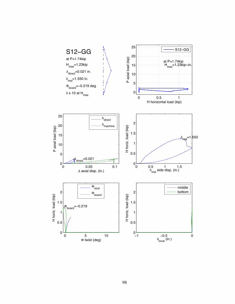
98
S12 GGat P=1.74kipHmax=1.23kip
direct=0.021 in.
mid=1.550 in.
board= 0.219 deg
x 10 at Hmax0 0.5 1
0
5
10
15
20
25
H horizontal load (kip)
P ax
ial l
oad
(kip
)
at P=1.74kip Hmax=1.23kip in.
S12 GG
0 0.05 0.10
5
10
15
20
25
axial disp. (in.)
P ax
ial l
oad
(kip
)
direct=0.021
direct
machine
0 0.5 1 1.50
0.5
1
1.5
2
mid side disp. (in.)
H h
oriz
. loa
d (k
ip)
mid=1.550
0 5 100
0.5
1
1.5
2
twist (deg)
H h
oriz
. loa
d (k
ip)
board= 0.219
stud
board
1 0.5 00
0.5
1
1.5
2
local (in.)
H h
oriz
. loa
d (k
ip)
middlebottom

99
S13 BOat P=4.51kip
Hmax=1.08kip
direct=0.041 in.
mid=1.149 in.
board=1.264 deg
x 10 at Hmax0 0.5 1
0
5
10
15
20
25
H horizontal load (kip)
P a
xial
load
(kip
)
at P=4.51kip Hmax=1.08kip in.
S13 BO
0 0.05 0.1 0.15 0.20
5
10
15
20
25
axial disp. (in.)
P a
xial
load
(kip
)
direct=0.041
direct
machine
0 0.5 1 1.50
0.5
1
1.5
2
mid side disp. (in.)
H h
oriz
. loa
d (k
ip)
mid=1.149
0 0.5 10
0.5
1
1.5
2
twist (deg)
H h
oriz
. loa
d (k
ip)
board=1.264
stud
board
4 2 0
x 10 4
0
0.5
1
1.5
2
local (in.)
H h
oriz
. loa
d (k
ip)
middlebottom

100
S14 OBat P=6.50kip
Hmax=0.76kip
direct=0.067 in.
mid=1.477 in.
board= 0.001 deg
x 10 at Hmax0 0.2 0.4 0.6 0.8
0
5
10
15
20
25
H horizontal load (kip)
P a
xial
load
(kip
)
at P=6.50kip Hmax=0.76kip in.
S14 OB
0 0.1 0.2 0.30
5
10
15
20
25
axial disp. (in.)
P a
xial
load
(kip
)
direct=0.067
direct
machine
0 0.5 1 1.50
0.5
1
1.5
2
mid side disp. (in.)
H h
oriz
. loa
d (k
ip)
mid=1.477
0 2 4 6 80
0.5
1
1.5
2
twist (deg)
H h
oriz
. loa
d (k
ip)
board= 0.001
stud
board
8 6 4 2 0
x 10 3
0
0.5
1
1.5
2
local (in.)
H h
oriz
. loa
d (k
ip)
middlebottom

101
S15 OOat P=14.93kipHmax=1.34kip
direct=0.083 in.
mid=1.069 in.
board=0.363 deg
x 10 at Hmax0 0.5 1
0
5
10
15
20
25
H horizontal load (kip)
P ax
ial l
oad
(kip
)
at P=14.93kip Hmax=1.34kip in.
S15 OO
0 0.1 0.2 0.3 0.40
5
10
15
20
25
axial disp. (in.)
P ax
ial l
oad
(kip
)
direct=0.083
direct
machine
0 0.5 10
0.5
1
1.5
2
mid side disp. (in.)
H h
oriz
. loa
d (k
ip)
mid=1.069
0 0.2 0.4 0.60
0.5
1
1.5
2
twist (deg)
H h
oriz
. loa
d (k
ip)
board=0.363
stud
board
15 10 5 0 5x 10 3
0
0.5
1
1.5
2
local (in.)
H h
oriz
. loa
d (k
ip)
middlebottom

102
S16 GOat P=14.69kip
Hmax=1.14kip
direct=0.077 in.
mid=1.008 in.
board=0.895 deg
x 10 at Hmax0 0.5 1
0
5
10
15
20
25
H horizontal load (kip)
P a
xial
load
(kip
)
at P=14.69kip Hmax=1.14kip in.
S16 GO
0 0.1 0.2 0.3 0.40
5
10
15
20
25
axial disp. (in.)
P a
xial
load
(kip
)
direct=0.077
direct
machine
0 0.5 10
0.5
1
1.5
2
mid side disp. (in.)
H h
oriz
. loa
d (k
ip)
mid=1.008
0 1 2 3 40
0.5
1
1.5
2
twist (deg)
H h
oriz
. loa
d (k
ip)
board=0.895
stud
board
0 0.2 0.4 0.6 0.80
0.5
1
1.5
2
local (in.)
H h
oriz
. loa
d (k
ip)
middlebottom
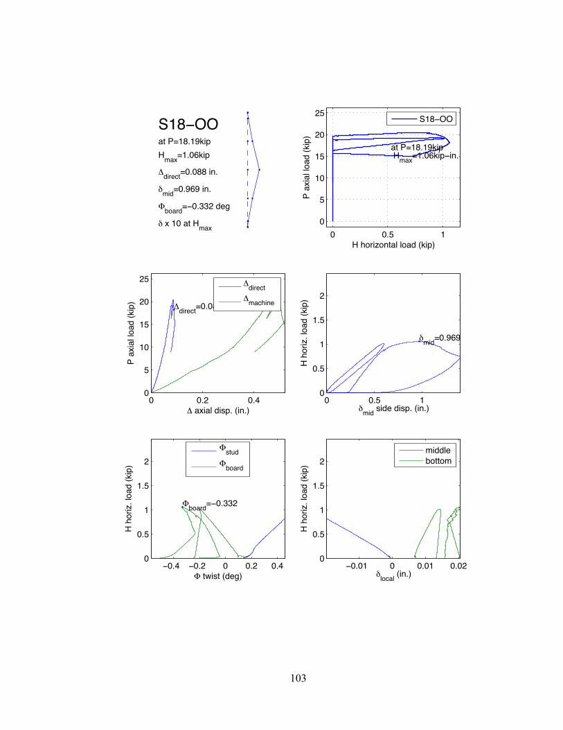
103
S18 OOat P=18.19kipHmax=1.06kip
direct=0.088 in.
mid=0.969 in.
board= 0.332 deg
x 10 at Hmax0 0.5 1
0
5
10
15
20
25
H horizontal load (kip)
P ax
ial l
oad
(kip
)
at P=18.19kip Hmax=1.06kip in.
S18 OO
0 0.2 0.40
5
10
15
20
25
axial disp. (in.)
P ax
ial l
oad
(kip
)
direct=0.088
direct
machine
0 0.5 10
0.5
1
1.5
2
mid side disp. (in.)
H h
oriz
. loa
d (k
ip)
mid=0.969
0.4 0.2 0 0.2 0.40
0.5
1
1.5
2
twist (deg)
H h
oriz
. loa
d (k
ip)
board= 0.332
stud
board
0.01 0 0.01 0.020
0.5
1
1.5
2
local (in.)
H h
oriz
. loa
d (k
ip)
middlebottom
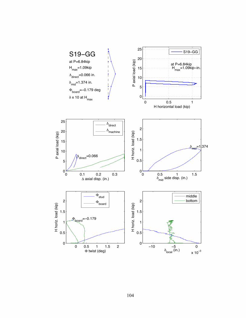
104
S19 GGat P=6.84kip
Hmax=1.09kip
direct=0.066 in.
mid=1.374 in.
board= 0.179 deg
x 10 at Hmax0 0.5 1
0
5
10
15
20
25
H horizontal load (kip)
P a
xial
load
(kip
)
at P=6.84kip Hmax=1.09kip in.
S19 GG
0 0.1 0.2 0.30
5
10
15
20
25
axial disp. (in.)
P a
xial
load
(kip
)
direct=0.066
direct
machine
0 0.5 1 1.50
0.5
1
1.5
2
mid side disp. (in.)
H h
oriz
. loa
d (k
ip)
mid=1.374
0 0.5 1 1.5 20
0.5
1
1.5
2
twist (deg)
H h
oriz
. loa
d (k
ip)
board= 0.179
stud
board
10 5 0
x 10 3
0
0.5
1
1.5
2
local (in.)
H h
oriz
. loa
d (k
ip)
middlebottom

105
S20 GGat P=11.61kipHmax=0.99kip
direct=0.063 in.
mid=0.994 in.
board= 0.158 deg
x 10 at Hmax0 0.5 1
0
5
10
15
20
25
H horizontal load (kip)
P ax
ial l
oad
(kip
)
at P=11.61kip Hmax=0.99kip in.
S20 GG
0 0.1 0.2 0.3 0.40
5
10
15
20
25
axial disp. (in.)
P ax
ial l
oad
(kip
)
direct=0.063
direct
machine
0 0.5 1 1.50
0.5
1
1.5
2
mid side disp. (in.)
H h
oriz
. loa
d (k
ip)
mid=0.994
0 1 2 30
0.5
1
1.5
2
twist (deg)
H h
oriz
. loa
d (k
ip)
board= 0.158
stud
board
15 10 5 0x 10 3
0
0.5
1
1.5
2
local (in.)
H h
oriz
. loa
d (k
ip)
middlebottom

106
S21 OBat P=9.92kipHmax=0.96kip
direct=0.060 in.
mid=0.901 in.
board= 0.001 deg
x 10 at Hmax0 0.5 1
0
5
10
15
20
25
H horizontal load (kip)
P ax
ial l
oad
(kip
)
at P=9.92kip Hmax=0.96kip in.
S21 OB
0 0.1 0.2 0.30
5
10
15
20
25
axial disp. (in.)
P ax
ial l
oad
(kip
)
direct=0.060
direct
machine
0 0.5 10
0.5
1
1.5
2
mid side disp. (in.)
H h
oriz
. loa
d (k
ip)
mid=0.901
3 2 1 00
0.5
1
1.5
2
twist (deg)
H h
oriz
. loa
d (k
ip)
board= 0.001
stud
board
15 10 5 0x 10 3
0
0.5
1
1.5
2
local (in.)
H h
oriz
. loa
d (k
ip)
middlebottom

107
S23 GGat P=14.42kip
Hmax=0.72kip
direct=0.082 in.
mid=1.080 in.
board=0.792 deg
x 10 at Hmax0 0.2 0.4 0.6 0.8
0
5
10
15
20
25
H horizontal load (kip)
P a
xial
load
(kip
)
at P=14.42kip Hmax=0.72kip in.
S23 GG
0 0.1 0.2 0.3 0.40
5
10
15
20
25
axial disp. (in.)
P a
xial
load
(kip
)
direct=0.082
direct
machine
0 0.5 1 1.50
0.5
1
1.5
2
mid side disp. (in.)
H h
oriz
. loa
d (k
ip)
mid=1.080
0 1 20
0.5
1
1.5
2
twist (deg)
H h
oriz
. loa
d (k
ip)
board=0.792
stud
board
15 10 5 0
x 10 3
0
0.5
1
1.5
2
local (in.)
H h
oriz
. loa
d (k
ip)
middlebottom

108
S26 BBat P=2.39kipHmax=0.59kip
direct=0.053 in.
mid=2.000 in.
board=0.002 deg
x 10 at Hmax0 0.2 0.4 0.6
0
5
10
15
20
25
H horizontal load (kip)
P ax
ial l
oad
(kip
)
at P=2.39kip Hmax=0.59kip in.
S26 BB
0 0.1 0.20
5
10
15
20
25
axial disp. (in.)
P ax
ial l
oad
(kip
)
direct=0.053
direct
machine
0 0.5 1 1.50
0.5
1
1.5
2
mid side disp. (in.)
H h
oriz
. loa
d (k
ip)
mid=2.000
0 10 20x 10 4
0
0.5
1
1.5
2
twist (deg)
H h
oriz
. loa
d (k
ip)
board=0.002
stud
board
0.4 0.2 00
0.5
1
1.5
2
local (in.)
H h
oriz
. loa
d (k
ip)
middlebottom
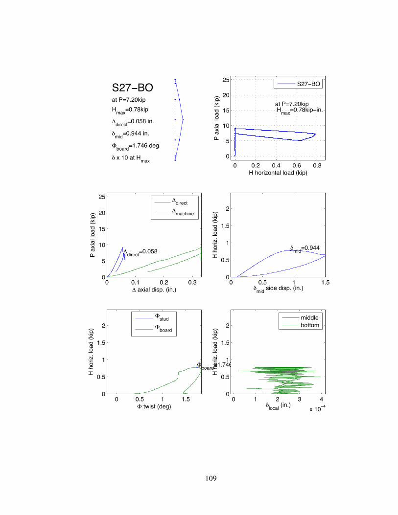
109
S27 BOat P=7.20kip
Hmax=0.78kip
direct=0.058 in.
mid=0.944 in.
board=1.746 deg
x 10 at Hmax0 0.2 0.4 0.6 0.8
0
5
10
15
20
25
H horizontal load (kip)
P a
xial
load
(kip
)
at P=7.20kip Hmax=0.78kip in.
S27 BO
0 0.1 0.2 0.30
5
10
15
20
25
axial disp. (in.)
P a
xial
load
(kip
)
direct=0.058
direct
machine
0 0.5 1 1.50
0.5
1
1.5
2
mid side disp. (in.)
H h
oriz
. loa
d (k
ip)
mid=0.944
0 0.5 1 1.50
0.5
1
1.5
2
twist (deg)
H h
oriz
. loa
d (k
ip)
board=1.746
stud
board
0 1 2 3 4
x 10 4
0
0.5
1
1.5
2
local (in.)
H h
oriz
. loa
d (k
ip)
middlebottom

110
S30 GGat P=14.67kip
Hmax=0.73kip
direct=0.071 in.
mid=0.909 in.
board= 0.485 deg
x 10 at Hmax0 0.2 0.4 0.6 0.8
0
5
10
15
20
25
H horizontal load (kip)
P a
xial
load
(kip
)
at P=14.67kip Hmax=0.73kip in.
S30 GG
0 0.1 0.2 0.3 0.40
5
10
15
20
25
axial disp. (in.)
P a
xial
load
(kip
)
direct=0.071
direct
machine
0 0.5 1 1.50
0.5
1
1.5
2
mid side disp. (in.)
H h
oriz
. loa
d (k
ip)
mid=0.909
0 1 2 3 40
0.5
1
1.5
2
twist (deg)
H h
oriz
. loa
d (k
ip)
board= 0.485
stud
board
10 5 0
x 10 3
0
0.5
1
1.5
2
local (in.)
H h
oriz
. loa
d (k
ip)
middlebottom

111
S31 OOat P=2.09kipHmax=2.14kip
direct=0.018 in.
mid=1.461 in.
board=0.263 deg
x 10 at Hmax0 0.5 1 1.5 2
0
5
10
15
20
25
H horizontal load (kip)
P ax
ial l
oad
(kip
)
at P=2.09kip Hmax=2.14kip in.
S31 OO
0 0.02 0.04 0.06 0.080
5
10
15
20
25
axial disp. (in.)
P ax
ial l
oad
(kip
)
direct=0.018
direct
machine
0 0.5 1 1.5 20
0.5
1
1.5
2
mid side disp. (in.)
H h
oriz
. loa
d (k
ip)
mid=1.461
0 0.5 10
0.5
1
1.5
2
twist (deg)
H h
oriz
. loa
d (k
ip)
board=0.263
stud
board
8 6 4 2 0x 10 3
0
0.5
1
1.5
2
local (in.)
H h
oriz
. loa
d (k
ip)
middlebottom
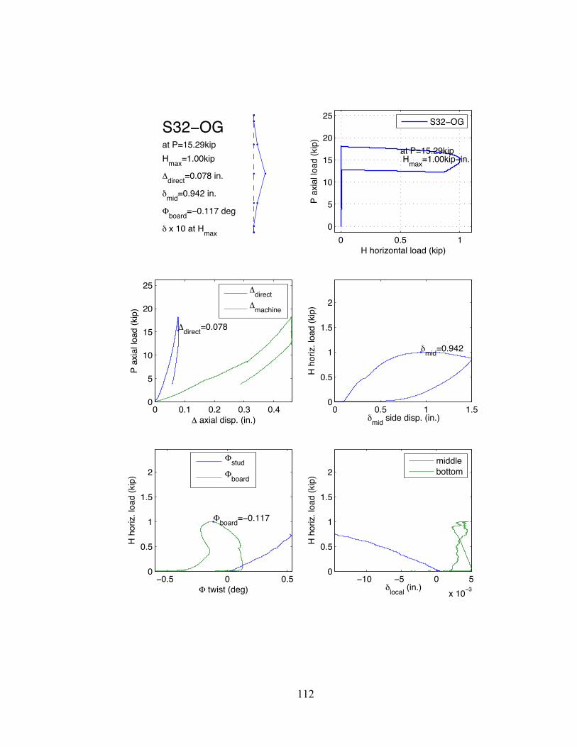
112
S32 OGat P=15.29kip
Hmax=1.00kip
direct=0.078 in.
mid=0.942 in.
board= 0.117 deg
x 10 at Hmax0 0.5 1
0
5
10
15
20
25
H horizontal load (kip)
P a
xial
load
(kip
)
at P=15.29kip Hmax=1.00kip in.
S32 OG
0 0.1 0.2 0.3 0.40
5
10
15
20
25
axial disp. (in.)
P a
xial
load
(kip
)
direct=0.078
direct
machine
0 0.5 1 1.50
0.5
1
1.5
2
mid side disp. (in.)
H h
oriz
. loa
d (k
ip)
mid=0.942
0.5 0 0.50
0.5
1
1.5
2
twist (deg)
H h
oriz
. loa
d (k
ip)
board= 0.117
stud
board
10 5 0 5
x 10 3
0
0.5
1
1.5
2
local (in.)
H h
oriz
. loa
d (k
ip)
middlebottom

113
S33 GOat P=1.82kip
Hmax=1.63kip
direct=0.025 in.
mid=1.794 in.
board=0.790 deg
x 10 at Hmax0 0.5 1 1.5
0
5
10
15
20
25
H horizontal load (kip)
P a
xial
load
(kip
)
at P=1.82kip Hmax=1.63kip in.
S33 GO
0 0.05 0.10
5
10
15
20
25
axial disp. (in.)
P a
xial
load
(kip
)
direct=0.025
direct
machine
0 0.5 1 1.5 20
0.5
1
1.5
2
mid side disp. (in.)
H h
oriz
. loa
d (k
ip)
mid=1.794
0 0.5 10
0.5
1
1.5
2
twist (deg)
H h
oriz
. loa
d (k
ip)
board=0.790
stud
board
10 5 0
x 10 3
0
0.5
1
1.5
2
local (in.)
H h
oriz
. loa
d (k
ip)
middlebottom

114
S34 BBat P=6.41kipHmax=0.54kip
direct=0.061 in.
mid=0.870 in.
board=0.002 deg
x 10 at Hmax0 0.2 0.4 0.6
0
5
10
15
20
25
H horizontal load (kip)
P ax
ial l
oad
(kip
)
at P=6.41kip Hmax=0.54kip in.
S34 BB
0 0.1 0.2 0.30
5
10
15
20
25
axial disp. (in.)
P ax
ial l
oad
(kip
)
direct=0.061
direct
machine
0 0.5 1 1.50
0.5
1
1.5
2
mid side disp. (in.)
H h
oriz
. loa
d (k
ip)
mid=0.870
0 0.5 1 1.5 2x 10 3
0
0.5
1
1.5
2
twist (deg)
H h
oriz
. loa
d (k
ip)
board=0.002
stud
board
3 2 1 0x 10 4
0
0.5
1
1.5
2
local (in.)
H h
oriz
. loa
d (k
ip)
middlebottom

115
S36 OGat P=10.14kip
Hmax=1.17kip
direct=0.064 in.
mid=1.212 in.
board=0.149 deg
x 10 at Hmax0 0.5 1
0
5
10
15
20
25
H horizontal load (kip)
P a
xial
load
(kip
)
at P=10.14kip Hmax=1.17kip in.
S36 OG
0 0.1 0.2 0.30
5
10
15
20
25
axial disp. (in.)
P a
xial
load
(kip
)
direct=0.064
direct
machine
0 0.5 1 1.5 20
0.5
1
1.5
2
mid side disp. (in.)
H h
oriz
. loa
d (k
ip)
mid=1.212
0 0.2 0.4 0.60
0.5
1
1.5
2
twist (deg)
H h
oriz
. loa
d (k
ip)
board=0.149
stud
board
15 10 5 0
x 10 3
0
0.5
1
1.5
2
local (in.)
H h
oriz
. loa
d (k
ip)
middlebottom

116
S37 BOat P=11.41kip
Hmax=0.73kip
direct=0.068 in.
mid=1.025 in.
board=1.675 deg
x 10 at Hmax0 0.2 0.4 0.6 0.8
0
5
10
15
20
25
H horizontal load (kip)
P a
xial
load
(kip
)
at P=11.41kip Hmax=0.73kip in.
S37 BO
0 0.1 0.2 0.30
5
10
15
20
25
axial disp. (in.)
P a
xial
load
(kip
)
direct=0.068
direct
machine
0 0.5 1 1.50
0.5
1
1.5
2
mid side disp. (in.)
H h
oriz
. loa
d (k
ip)
mid=1.025
0 1 2 30
0.5
1
1.5
2
twist (deg)
H h
oriz
. loa
d (k
ip)
board=1.675
stud
board
0 1 2 3 4
x 10 4
0
0.5
1
1.5
2
local (in.)
H h
oriz
. loa
d (k
ip)
middlebottom

117
S38 OOat P=11.45kipHmax=1.50kip
direct=0.062 in.
mid=1.138 in.
board= 0.807 deg
x 10 at Hmax0 0.5 1 1.5
0
5
10
15
20
25
H horizontal load (kip)
P ax
ial l
oad
(kip
)
at P=11.45kip Hmax=1.50kip in.
S38 OO
0 0.1 0.2 0.3 0.40
5
10
15
20
25
axial disp. (in.)
P ax
ial l
oad
(kip
)
direct=0.062
direct
machine
0 0.5 1 1.50
0.5
1
1.5
2
mid side disp. (in.)
H h
oriz
. loa
d (k
ip)
mid=1.138
0.8 0.6 0.4 0.2 0 0.2 0.40
0.5
1
1.5
2
twist (deg)
H h
oriz
. loa
d (k
ip)
board= 0.807
stud
board
15 10 5 0 5x 10 3
0
0.5
1
1.5
2
local (in.)
H h
oriz
. loa
d (k
ip)
middlebottom

118
S39 GGat P=17.38kip
Hmax=0.76kip
direct= 0.384 in.
mid=0.878 in.
board=0.326 deg
x 10 at Hmax0 0.2 0.4 0.6 0.8
0
5
10
15
20
25
H horizontal load (kip)
P a
xial
load
(kip
)
at P=17.38kip Hmax=0.76kip in.
S39 GG
0 0.1 0.2 0.3 0.40
5
10
15
20
25
axial disp. (in.)
P a
xial
load
(kip
)
4
direct
machine
0 0.5 10
0.5
1
1.5
2
mid side disp. (in.)
H h
oriz
. loa
d (k
ip)
mid=0.878
2 1 0 1 20
0.5
1
1.5
2
twist (deg)
H h
oriz
. loa
d (k
ip)
board=0.326
stud
board
0.02 0.015 0.01 0.005 00
0.5
1
1.5
2
local (in.)
H h
oriz
. loa
d (k
ip)
middlebottom

119
CURRICULUM VITA
Kara Peterman was born in Palo Alto, California and grew up in Hong Kong SAR and
Fairfax, Virginia. She attended Swarthmore College in Swarthmore, PA, graduating in
2009 with a BS in Engineering and a minor in Statistics. Kara is currently pursuing her
PhD at Johns Hopkins University in Baltimore, MD. Her PhD work focuses on the
performance-based seismic design of cold-formed steel structures.


