

Abstract
TYNER, DAVID WADE. Evaluation of Repellent Finishes Applied by Atmospheric Plasma. (Under the direction of Dr. Peter J. Hauser.)
The conventional pad-dry-cure method to impart a water repellent fluoropolymer
finish onto a textile has been used effectively for many years. Although this process has
been very successful and is the most common method of repellent finishing, it does have
disadvantages. The largest draw back to this method is that it is a wet process requiring high
levels of thermal energy to evaporate the water and cure the fluoropolymer.
Plasma processing can also impart a repellent finish on a textile and does not require
high levels of thermal energy because there is no water to evaporate and the fluoropolymer
polymerizes in the plasma therefore it does not need to be cured. Until recently, plasmas for
industrial processing were only available under reduced pressure. This limited
manufacturing because of the high cost of the vacuum equipment and the limitations of batch
processing.
Plasma processing is now available at atmospheric pressure resulting in the ability to
polymerize a water repellent fluoropolymer onto the surface of a textile in a continuous full
width process. This process has been successful in research labs although there has been
very little research conducted on fabrics treated with industrial machinery. This research
studied the repellency, durability, and cost associated with Dow Corning Plasma Solution’s
(DCPS) Atmospheric Pressure Plasma Liquid Deposition (APPLD) technology and the
conventional pad-dry-cure method. The core objective of this project was to determine if the
APPLD process could be a viable replacement for the conventional pad-dry-cure method at
this current state of technology for the cotton, nylon, polyester, and polyester/cotton fabrics

tested in this research. It should be noted that the fluoropolymers used in the conventional
and plasma treatments are not the same and the environmental impact of the plasma
treatment is not known at this time.
Spray, impact, water/alcohol, oil, and contact angle tests suggested that all fabrics
treated by the atmospheric plasma process exhibited equal levels of water repellency as a
commercial product finished by the conventional pad-dry-cure method. Only the cotton and
polyester/cotton fabrics treated by atmospheric plasma showed a decrease in repellency after
multiple wash cycles when compared to the conventional finishes under identical washings.
This research has also taken an in depth look at the costs associated with both the
atmospheric plasma and the conventional processing methods. It has been determined that
the atmospheric plasma cost associated with the fabric used in this research was $1.13 per
square yard. It was also calculated that the cost to finish a square yard of the fabric by the
conventional method was $0.20. Although this is a large discrepancy, a theoretical cost
projection for the DCPS APPLD process in a fully engineered industrial scenario was
estimated at $0.15 per square yard.
The results of this research have lead to two main recommendations for future
research. First, additional fabric should be run by Dow Corning at settings from which the
theoretical cost calculation was based, which more accurately portrays an industrial scenario
in order to determine if comparable results will be observed. Secondly, a company named
APJeT should be investigated because they also have a continuous full width atmospheric
plasma machine and have the following differences from Dow Corning: APJeT can recycle
the helium gas used in the process, can coat different finishes on each side of the fabric, and

has the ability to run faster because of a higher plasma density, leading to a projected cost per
square yard of fabric of $0.10.
EVALUATION OF REPELLENT FINISHES APPLIED BY ATMOSPHERIC
PLASMA
by
DAVID WADE TYNER
A thesis submitted to the Graduate Faculty of
North Carolina State University
in partial fulfillment of the
Degree of Master of Science
TEXTILE ENGINEERING
Raleigh, NC
2007
APPROVED BY:
____________________________
Dr. Peter J. Hauser
Chair of Advisory Committee
____________________________
Dr. Stephen Michielsen
Member of Advisory Committee
____________________________
Dr. Henry Boyter Jr.
Member of Advisory Committee
____________________________
Dr. Jeffrey A. Joines
Member of Advisory Committee

ii
Dedication
This work is dedicated to my wife Jaclyn who supported and encouraged me to attend
graduate school. During my time at NCSU, she has given me a beautiful daughter who has
put my studies in perspective and to which I am deeply grateful.

iii
Biography
Wade Tyner was born and raised just outside of Athens, Ga. After graduating from
Madison County High school, Wade accepted an athletic scholarship to attend West Virginia
University where he studied Electrical Engineering. He graduated in May of 2003 with cum
laude honors while obtaining All-American status all four years while shooting for WVU’s
renowned rifle team. Wade accepted a position in plant engineering at Milliken &
Company’s Excelsior Union Finishing plant in Union, SC in July of the same year. His wife,
Jaclyn, has a master’s degree in counseling and was working as a counselor at Mount Olive
College at Research Triangle Park until the birth of Aubrey Gale Tyner on June 14, 2006.
After graduation from NCSU, Wade will be returning to Milliken & Company to pursue a
career in nonwovens.

iv
Acknowledgements
This work could not be completed without the help of many people. First, I would
like to thank Milliken & Company along with the Institute of Textile Technology for giving
me the opportunity to return to school to earn my masters degree. Secondly, I would like to
thank all of my committee members for sharing with me their knowledge of my subject and
giving me direction along with constructive criticism. Thirdly, I would like to thank the
following individuals that also have contributed to my research:
Alex Padilla, APJeT
Allen White, Milliken & Co.
Angie Brantley, NCSU
Mary Ann Ankeny, Cotton Inc.
Bob Adams, Milliken & Co.
Chris Desoiza, Milliken & Co.
David Wenstrup, Milliken & Co.
Fred Stevie, NCSU
Gary Lord, Dow Corning
Caroline O’Sullivan, Dow Corning
Jan Pegram, NCSU
Jeff Krauss, NCSU
Jack Daniels, AATCC
Paul Pruitt, Milliken & Co.
David Beard, Milliken & Co.
Joe Waddell, Milliken & Co.
Joel White, IT3
Judy Elson, NCSU
Hoonjoo Lee, NCSU
Manfred Young, ITG
Nathan Miller, Cotton Inc.
Shelly Benjamin, Milliken & Co.
Steve Middlebrook, Milliken & Co.
Suzanne Holmes, AATCC
Svetlana Verenich, NCSU
Patrice Hill, ITT
Chris Moses, ITT
Suzanne Matthews, Whitford

v
Table of Contents List of Figures ....................................................................................................................................... ix List of Tables.......................................................................................................................................... x List of Equations .................................................................................................................................xiii
1. Background .................................................................................................................................... 1 2. Literature Review ........................................................................................................................... 3
2.1 Introduction ............................................................................................................................ 3 2.2 Water Repellency ................................................................................................................... 3
2.2.1 Concepts ......................................................................................................................... 4 2.2.2 Wetting ........................................................................................................................... 4 2.2.3 Contact Angles ............................................................................................................... 7 2.2.4 Critical Surface Tension ................................................................................................. 9 2.2.5 Fabric Construction ...................................................................................................... 12
2.3 Water Repellents .................................................................................................................. 14 2.3.1.1 Non Silicone and Non Fluorocarbon Finishes.......................................................... 14 2.3.1.2 Silicone Finishes....................................................................................................... 16 2.3.1.3 Fluorochemical Finishes........................................................................................... 19
2.4 Test Methods ........................................................................................................................ 22 2.4.1 Spray Test..................................................................................................................... 22 2.4.2 Impact Test ................................................................................................................... 23 2.4.3 Rain Test....................................................................................................................... 23 2.4.4 Hydrostatic Pressure Test ............................................................................................. 23 2.4.5 Sorption Tests............................................................................................................... 24
2.5 Repellent Finishing............................................................................................................... 24 2.5.1 Conventional Methods.................................................................................................. 25
2.5.1.1 Exhaustion ................................................................................................................ 25 2.5.1.2 Padding..................................................................................................................... 25 2.5.1.3 Spraying.................................................................................................................... 27 2.5.1.4 Foaming.................................................................................................................... 27 2.5.1.5 Drying....................................................................................................................... 28

vi
2.5.1.6 Curing....................................................................................................................... 28 2.5.2 Plasma Processes .......................................................................................................... 29
2.5.2.1 Vacuum Plasmas ...................................................................................................... 32 2.5.2.2 Atmospheric ............................................................................................................. 34
2.6 Conclusion............................................................................................................................ 38 3. Procedures & Methodology.......................................................................................................... 39
3.1 Introduction .......................................................................................................................... 39 3.2 Fabrics Tested....................................................................................................................... 40
3.2.1 Cotton ........................................................................................................................... 40 3.2.2 65/35 Polyester/Cotton ................................................................................................. 41 3.2.3 Polyester ....................................................................................................................... 43 3.2.4 Nylon ............................................................................................................................ 44 3.2.5 Nonwovens ................................................................................................................... 45
3.3 Repellency Tests................................................................................................................... 46 3.3.1 Spray............................................................................................................................. 46 3.3.2 Impact ........................................................................................................................... 48 3.3.3 Water/Alcohol .............................................................................................................. 48 3.3.4 Oil ................................................................................................................................. 50 3.3.5 Contact Angle............................................................................................................... 51 3.3.6 Additional Tests............................................................................................................ 52
3.3.6.1 Hydrostatic Pressure ................................................................................................. 52 3.3.6.2 Wash Shrinkage........................................................................................................ 52 3.3.6.3 Air Permeability ....................................................................................................... 53 3.3.6.4 Tensile ...................................................................................................................... 53
3.4 Durability Tests .................................................................................................................... 53 3.4.1 X-ray Photoelectron Spectroscopy ............................................................................... 54 3.4.2 Wash............................................................................................................................. 54
4. Results and Discussions ............................................................................................................... 58 4.1 Atmospheric Plasma Treatment ........................................................................................... 58 4.2 Repellency & Durability....................................................................................................... 61
4.2.1 Cotton ........................................................................................................................... 61

vii
4.2.1.1 XPS Analysis............................................................................................................ 61 4.2.1.2 Spray......................................................................................................................... 62 4.2.1.3 Impact ....................................................................................................................... 63 4.2.1.4 Water/Alcohol .......................................................................................................... 64 4.2.1.5 Oil ............................................................................................................................. 64 4.2.1.6 Water Contact Angle ................................................................................................ 65
4.2.2 Polyester/Cotton ........................................................................................................... 66 4.2.2.1 XPS Analysis............................................................................................................ 67 4.2.2.2 Spray......................................................................................................................... 68 4.2.2.3 Impact ....................................................................................................................... 69 4.2.2.4 Water/Alcohol .......................................................................................................... 70 4.2.2.5 Oil ............................................................................................................................. 71 4.2.2.6 Water Contact Angle ................................................................................................ 71
4.2.3 Polyester ....................................................................................................................... 73 4.2.3.1 XPS Analysis............................................................................................................ 73 4.2.3.2 Spray......................................................................................................................... 74 4.2.3.3 Impact ....................................................................................................................... 75 4.2.3.4 Water/Alcohol .......................................................................................................... 76 4.2.3.5 Oil ............................................................................................................................. 76 4.2.3.6 Water Contact Angle ................................................................................................ 77 4.2.3.7 Additional Tests........................................................................................................ 78
4.2.4 Nylon ............................................................................................................................ 84 4.2.4.1 XPS Analysis............................................................................................................ 85 4.2.4.2 Spray......................................................................................................................... 86 4.2.4.3 Impact ....................................................................................................................... 86 4.2.4.4 Water/Alcohol .......................................................................................................... 87 4.2.4.5 Oil ............................................................................................................................. 88 4.2.4.6 Water Contact Angle ................................................................................................ 88
4.3 Cost Analysis........................................................................................................................ 90 4.3.1 Conventional Pad-Dry-Cure Finishing......................................................................... 90 4.3.2 Atmospheric Pressure Plasma Liquid Deposition Finishing ........................................ 91

viii
4.3.2.1 Theoretical Cost Projection ...................................................................................... 92 5. Conclusions & Recommendations ............................................................................................... 96
5.1 Repellency and Durability .................................................................................................... 96 5.2 Cost....................................................................................................................................... 97 5.3 Recommendations ................................................................................................................ 98 5.4 Summary ............................................................................................................................ 101
6. List of References....................................................................................................................... 102 7. Appendices ................................................................................................................................. 108
Appendix A : Dow Corning’s Atmospheric Pressure Plasma Liquid Deposition.............. 109 Appendix B : X-ray Photoelectron Spectroscopy (XPS) .................................................. 113
Appendix C : Cotton Additional Tables and Figures........................................................ 115
Appendix D : Polyester/Cotton Additional Tables and Figures........................................ 120
Appendix E : Polyester Additional Tables and Figures .................................................... 131
Appendix F : Nylon Additional Tables and Figures ......................................................... 173
Appendix G : Conventional Finish Cost Analysis Calculations ........................................ 184
Appendix H : APPLD Cost Analysis Calculations ............................................................ 189
Appendix I : Chemical Material Safety Data Sheets......................................................... 192

ix
List of Figures Figure 2.1. Equilibrium Contact Angle ................................................................................................. 7 Figure 2.2. Determination of Critical Surface Tension ....................................................................... 10 Figure 2.3. Three Possible Types of Behavior of a Liquid in Contact with a Surface ........................ 12 Figure 2.4. Polysiloxane Chemical Structure ...................................................................................... 16 Figure 2.5. Polymethylhydrogensiloxane (top) and Polydimethylsiloxane (bottom).......................... 17 Figure 2.6. Chemical Structures of Silanol (left) and Silane (right).................................................... 17 Figure 2.7. Schematic of Commercial Silicone Water Repellent........................................................ 18 Figure 3.1. Spray Test Ratings ............................................................................................................ 47 Figure 3.2. AATCC TM 193 Solution Grades .................................................................................... 49 Figure 4.1. Chemical Precursors Used for APPLD Treatment............................................................ 58 Figure 7.1. APPLD Precursor Injection Apparatus (Taken From WO Patent 28548) ...................... 109 Figure 7.2. Continuous APPLD Treatment (Taken from WO Patent 59809) ................................... 110 Figure 7.3. DCPS SE-1100 LabLine Machine .................................................................................. 111 Figure 7.4. DCPS SE-1000 AP4 Machine......................................................................................... 112

x
List of Tables Table 2.1. Critical Surface Tensions and Surface Free Energies of Polymers .................................... 11 Table 2.2. Surface Tension Values of Water, Critical Surface Energies of Selected Surfaces ........... 11 Table 2.3. Surface Tension Values of Surfaces Composed of Fluorocarbons .................................... 20 Table 2.4. Physicochemical Techniques ............................................................................................. 30 Table 3.1. Cotton Fabric Construction ................................................................................................ 40 Table 3.2. Cotton Fluorochemical Bath .............................................................................................. 41 Table 3.3. Polyester/Cotton Fabric Construction ................................................................................ 41 Table 3.4. Polyester/Cotton Repellency Requirements ....................................................................... 43 Table 3.5. Polyester Fabric Construction ............................................................................................ 43 Table 3.6. Polyester Additional Requirements.................................................................................... 44 Table 3.7. Nylon Fabric Construction ................................................................................................. 44 Table 3.8. Nylon Repellency Requirements........................................................................................ 45 Table 3.9. AATCC TM 193 Standard Test Liquids ............................................................................ 49 Table 3.10. AATCC TM 118 Standard Test Liquids .......................................................................... 51 Table 3.11. Number of Samples Required for Each Fabric................................................................. 55 Table 3.12. Wash Equipment .............................................................................................................. 55 Table 3.13. Washing Machine Settings ............................................................................................... 56 Table 3.14. Dryer Machine Settings.................................................................................................... 56 Table 4.1. DCPS APPLD DOE Operating Conditions........................................................................ 59 Table 4.2. DCPS LabLine Machine Settings....................................................................................... 59 Table 4.3. Optimal Parameters for Additional Nylon Treatment ........................................................ 60 Table 4.4. Cotton Fabric Nomenclature .............................................................................................. 61 Table 4.5. Fluorine Composition of Cotton Segments ........................................................................ 62 Table 4.6. Cotton Spray Results .......................................................................................................... 62 Table 4.7. Cotton Impact Penetration Results ..................................................................................... 63 Table 4.8. Cotton Water/Alcohol Results............................................................................................ 64 Table 4.9. Cotton Oil Results .............................................................................................................. 65 Table 4.10. Cotton Contact Angle Results .......................................................................................... 65 Table 4.11. Polyester/Cotton Fabric Nomenclature ............................................................................ 67 Table 4.12. Fluorine Composition of Polyester/Cotton Segments ...................................................... 67

xi
Table 4.13. Polyester/Cotton Spray Results ........................................................................................ 68 Table 4.14. Polyester/Cotton Impact Penetration Results ................................................................... 69 Table 4.15. Polyester/Cotton Water/Alcohol Results.......................................................................... 70 Table 4.16. Polyester/Cotton Oil Results ............................................................................................ 71 Table 4.17. Polyester/Cotton Contact Angle Results .......................................................................... 72 Table 4.18. Polyester Fabric Nomenclature ........................................................................................ 73 Table 4.19. Fluorine Composition of Polyester Segments .................................................................. 74 Table 4.20. Polyester Spray Results .................................................................................................... 75 Table 4.21. Polyester Impact Penetration Results ............................................................................... 75 Table 4.22. Polyester Water/Alcohol Results...................................................................................... 76 Table 4.23. Polyester Oil Results ........................................................................................................ 77 Table 4.24. Polyester Contact Angle Results ...................................................................................... 77 Table 4.25. Polyester Hydrostatic Pressure Results ............................................................................ 79 Table 4.26. Polyester 5 Wash Shrinkage Results ................................................................................ 80 Table 4.27. Polyester Air Permeability Results................................................................................... 81 Table 4.28. Polyester Tensile Test Results in the Warp Direction...................................................... 83 Table 4.29. Polyester Tensile Test Results in the Fill Direction ......................................................... 83 Table 4.30. Nylon Fabric Nomenclature ............................................................................................. 85 Table 4.31. Fluorine Composition of Nylon Segments ....................................................................... 85 Table 4.32. Nylon Spray Results ......................................................................................................... 86 Table 4.33. Nylon Impact Penetration Results .................................................................................... 87 Table 4.34. Nylon Water/Alcohol Results........................................................................................... 87 Table 4.35. Nylon Oil Results ............................................................................................................. 88 Table 4.36. Nylon Contact Angle Results ........................................................................................... 89 Table 4.37. Total Cost of Conventional Treatment ............................................................................. 90 Table 4.38. Total Cost of APPLD Treatment...................................................................................... 91 Table 4.39. Fluorine Analysis Test Results......................................................................................... 93 Table 4.40. Total Theoretical Cost of APPLD Treatment in an Industrial Scenario........................... 95 Table 5.1. Comparison of Dow Corning and APJeT Technologies .................................................. 101 Table 7.1. Conventional Chemical Cost per Pound........................................................................... 184 Table 7.2. Information Used by American Monforts ........................................................................ 187
xii
Table 7.3. Information Returned by American Monforts.................................................................. 187 Table 7.4. Price of Chemical Precursors ........................................................................................... 189

xiii
List of Equations Equation 2.1. Gibbs Equation................................................................................................................ 4 Equation 2.2. Spontaneous Wetting ...................................................................................................... 5 Equation 2.3. Work of Immersion and Penetration ............................................................................... 5 Equation 2.4. Dupré’s Equation ............................................................................................................ 6 Equation 2.5. Work of Spreading .......................................................................................................... 6 Equation 2.6. Young’s Equation ........................................................................................................... 7 Equation 2.7. Work of Adhesion........................................................................................................... 8 Equation 2.8. Hydrostatic Pressure ..................................................................................................... 13 Equation 2.9. Percent Wet Pick Up..................................................................................................... 25 Equation 4.1. Fluorine ppm Levels on Cotton (top) and Polyester (bottom) ...................................... 93 Equation 7.1. Weight of Conventional Bath Picked Up.................................................................... 184 Equation 7.2. Conventional Chemicals Picked Up............................................................................ 185 Equation 7.3. Conventional Chemical Cost....................................................................................... 186 Equation 7.4. Tenter Electricity Cost ................................................................................................ 188 Equation 7.5. Natural Gas Cost to Maintain Tenter at 350 °F........................................................... 188 Equation 7.6. Natural Gas Cost to Dry and Cure .............................................................................. 188 Equation 7.7. APPLD Electricity Cost .............................................................................................. 190 Equation 7.8. APPLD Helium Cost................................................................................................... 190 Equation 7.9. Mass of Precursor Injected into Plasma Region.......................................................... 191 Equation 7.10. Mass of Precursor on Fabric ..................................................................................... 191 Equation 7.11 . Cost of Chemical Precursors.................................................................................... 191

1
1. Background
Atmospheric plasma treatment of textile materials to obtain water repellency has
recently become available to industry in a full width continuous process. This project will
study the repellency, durability, and cost of fluoropolymer textiles treated with atmospheric
plasma in comparison to the conventional pad-dry-cure process. The core objective of this
study is to determine if the current pad-dry-cure process can be replaced with an atmospheric
plasma process having an equivalent or superior performance at a comparable cost.
Although there is evidence that an atmospheric plasma process can achieve
repellency in textiles, there is currently no cost projection available for this process on an
industrial scale. In order to determine if atmospheric plasma finishing is a practical
alternative to conventional pad-dry-cure finishing, the cost of the former must be identified.
A conventional pad-dry-cure process requires high levels of thermal energy to
evaporate water and cure the fluoropolymer. In an industrial process, the energy needed to
dry the fabric is extremely expensive. In addition, intermediate fluorochemicals that are used
to produce these fluoropolymers have recently been shown to be persistently present in the
environment. Concerns of danger to public health from these intermediates have prompted
extensive review of existing commercial repellent finishes and renewed interest in the search
for new chemicals and application methods for producing repellent textiles.
The atmospheric plasma process is a dry process at room temperature where neither
water nor drying energy is needed. Atmospheric plasma machines are relatively small and

2
can easily be placed as a step within an in-line continuous process. In addition, atmospheric
plasma applied repellent finishes can involve different hydrophobic reactants that have not
been shown to be environmentally hazardous. The fluorochemicals used in the atmospheric
plasma treatment for this research were different from the chemicals used in the conventional
pad-dry-cure method. In addition, it should be noted that the chemicals used in the
atmospheric plasma process in this research were not used to represent an environmentally
friendly fluorochemical replacement for conventional fluorochemical pad-dry-cure
processing.
The objective of this research problem is to determine if atmospheric plasma is a
practical alternative to conventional pad-dry-cure repellent finishing at this current state of
technology. In order to address this objective, this research will evaluate the effectiveness of
both processes relative to repellency and durability, and also associate a cost to both the pad-
dry-cure and atmospheric plasma processes.

3
2. Literature Review
2.1 Introduction
The purpose of this literature review is to establish what is already known about the
concepts of liquid repellency and the use of atmospheric plasma treatment on textiles. The
theory of liquid repellency will be investigated along with methods used to make textile
fabrics repellent. The physics of plasma processing will not be covered in depth although the
results from plasma treatments will be reviewed. For more information on the physics of
plasma processing, the reader is referred to a book by M. Lieberman and A. Lichtenburg
called Principles of Plasma Discharges and Materials Processing.1
The review is broken into two main sections. The first section will discuss repellency
including theory, chemicals, and test methods. The second section will discuss the methods
used in repellent textile finishing including the conventional processes, such as pad-dry-cure,
and plasma processes, both low pressure and atmospheric.
2.2 Water Repellency
This chapter will discuss the theory of water repellents, typical chemical finishes to
obtain water repellency, and tests that can be used in order to quantify liquid repellency.
Although this section will discuss water repellency, the concepts, chemicals, and test
methods can also apply to other liquids including oils.
Water repellent treatment of fabrics has been of great interest since at least the
1880s.2 By definition, fabrics with water repellent finishes will repel water. The repulsion of
4
water from the fabric surface is due to the resistance of wetting, absorption, or penetration of
the water or any combination of these. Many terms have been used for water repellent
fabrics, particularly in marketing2, that are often imprecise, such as the term “water proof”.
Water proofing of textile fabrics will provide a barrier not only to water, but to water
vapor as well. Water repellent textile fabrics provide a barrier to water in the form of a
liquid, such as a rain drop, but allow water vapor to escape the fabric. Such water repellent
“breathable” textiles provide a much greater value to the consumer than water proof textiles.
Care should be taken to make the distinction between water proof and water repellent
textiles. This review will focus only on water repellency.
2.2.1 Concepts
In order to understand the mechanisms of water repellency, the physical interactions
at the surface of the fiber must be understood. Once these mechanisms are understood, the
likelihood of a fabric being wetted by a liquid can be predicted and fabrics can be engineered
to meet water repellency specifications.
2.2.2 Wetting
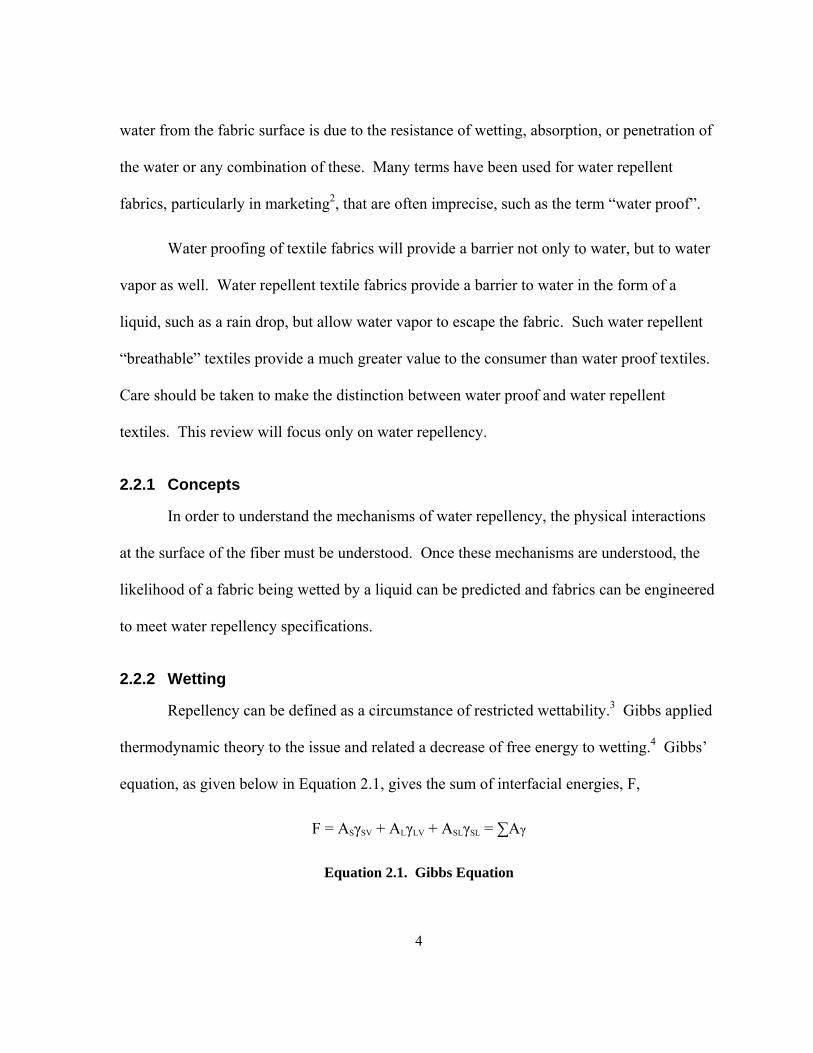
Repellency can be defined as a circumstance of restricted wettability.3 Gibbs applied
thermodynamic theory to the issue and related a decrease of free energy to wetting.4 Gibbs’
equation, as given below in Equation 2.1, gives the sum of interfacial energies, F,
F = ASγSV + ALγLV + ASLγSL = ∑Aγ
Equation 2.1. Gibbs Equation

5
where A is the area of subscripts S, L, and V that represent solid, liquid, and gas respectively
while γ is the surface energy per unit area. Spontaneous wetting occurs when the change in
free energy, ΔF, becomes negative as the result of a liquid-solid contact. Gibbs presented
this in Equation 2.2 below as:
ΔF = F2-F1 = Σ(Aγ)2 - Σ(Aγ)1
Equation 2.2. Spontaneous Wetting
where F1 and F2 are the sum of the interfacial energies before and after the liquid-solid
contact respectively. As a liquid is introduced to a surface, the solid-vapor interface is
replaced by a liquid-vapor interface. The change of the surface interface by a liquid can be
achieved by work done on the surface by immersion, capillary sorption, adhesion, and
spreading.2, 3 The work of immersion, adhesion, and spreading is denoted as WI, WA, and
WS respectively, while the work of capillary sorption is commonly known as the work of
penetration (WP). Depending on the means of wetting, the free energy change when a liquid
is removed from a solid will yield WI if the solid was immersed in a liquid, or WP if the
liquid was absorbed into the solid, which in our case is a textile.3 This concept is given in
Equation 2.3 below.
WI = WP = γSV - γSL
Equation 2.3. Work of Immersion and Penetration
For a surface to be repellent, WI (or possibly WP) must be negative.3 In other words,
it is desirable for the interfacial energy between a solid and vapor (γSV) to be smaller than the
6
interfacial energy of the solid and liquid interface (γSL). From this, it can be concluded that a
surface with a very low interfacial energy relative to vapor (γSV) is desirable for repellency.
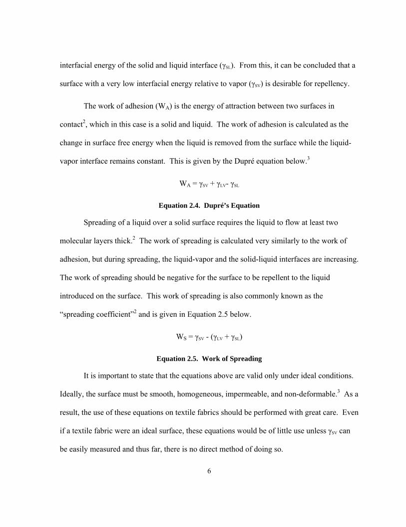
The work of adhesion (WA) is the energy of attraction between two surfaces in
contact2, which in this case is a solid and liquid. The work of adhesion is calculated as the
change in surface free energy when the liquid is removed from the surface while the liquid-
vapor interface remains constant. This is given by the Dupré equation below.3
WA = γSV + γLV- γSL
Equation 2.4. Dupré’s Equation
Spreading of a liquid over a solid surface requires the liquid to flow at least two
molecular layers thick.2 The work of spreading is calculated very similarly to the work of
adhesion, but during spreading, the liquid-vapor and the solid-liquid interfaces are increasing.
The work of spreading should be negative for the surface to be repellent to the liquid
introduced on the surface. This work of spreading is also commonly known as the
“spreading coefficient”2 and is given in Equation 2.5 below.
WS = γSV - (γLV + γSL)
Equation 2.5. Work of Spreading
It is important to state that the equations above are valid only under ideal conditions.
Ideally, the surface must be smooth, homogeneous, impermeable, and non-deformable.3 As a
result, the use of these equations on textile fabrics should be performed with great care. Even
if a textile fabric were an ideal surface, these equations would be of little use unless γSV can
be easily measured and thus far, there is no direct method of doing so.

7
2.2.3 Contact Angles
If a liquid is neither immediately absorbed nor spread along the surface of a solid, the
drop will take a definite shape as the liquid, vapor, and solid interfaces reach equilibrium.
The angle from the solid-liquid interface to the liquid-vapor tangent is defined as the contact
angle θ and shown below in Figure 2.1.
Figure 2.1. Equilibrium Contact Angle
In the middle of the nineteenth century, Young related the contact angle to
wettability.5 High values of the contact angle θ indicate repellency, or more technically poor
wettability.2 Young proposed that a drop similar to that in Figure 2.1 would be subject to the
equilibrium forces given in Equation 2.6 below.
γSV = γSL + γLV cos θ
Equation 2.6. Young’s Equation
Young’s equation brings us closer to being able to measure the work performed on a
surface in order to determine repellency. When Equation 2.6 is combined with Equation 2.4,
Equation 2.7 below is derived.

8
WA = (γSL + γLV cos θ)+ γLV - γSL = γLV cos θ
Equation 2.7. Work of Adhesion
Equation 2.7 is practical for use because both γLV and cos θ are measurable.2
Although relative wettability can be determined from a measured contact angle, caution
should be used because Young’s equation, Equation 2.6, is only valid for an equilibrium
contact angle. In a real system, the liquid will typically recede or advance.
In order to explore receding and advancing contact angles, assume that a rain drop
falls on the surface of a water repellent fabric. The initial force of the drop hitting the fabric
will cause the drop to deform and temporarily spread on the fabric. The drop will then
recede from the fabric and form a droplet with a measurable contact angle. The measured
contact angle would be lower than that of a droplet that was gently placed on the fabric. This
is because during the initial spreading of the water, the surface absorbed some of the liquid
and thereby changed the surface tension upon recession of the droplet.6
The difference between advancing and receding contact angles is expressed by
contact angle hysteresis.3 Contact angle hysteresis is also dependent on surface
inconsistencies7 or surface roughness.8 The works of Adam, Fowks, and Wenzel show that
water repellent surfaces must be prepared with great care before the application of a water
repellent finish so that surface homogeneity and smoothness can be achieved.3 This is a
major challenge for textiles, and explains why there is such variability in repellency
performance results with fabrics.2

9
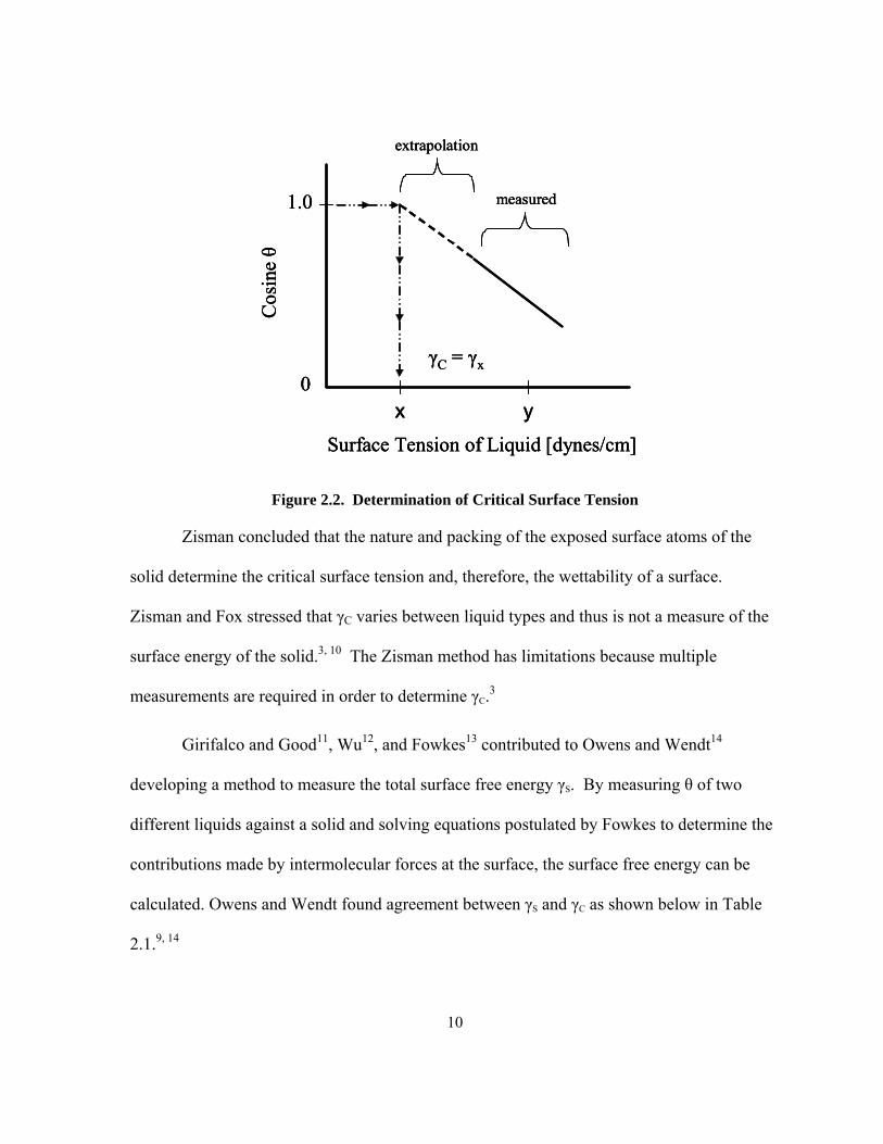
2.2.4 Critical Surface Tension
In order to predict the wettability of a surface, scientists knew that they would have to
find a way to calculate the surface free energy of a solid. Zisman developed a critical surface
tension (γC) where only liquids having surface tensions above this value will be repelled by
the surface.9 Zisman came to this conclusion by taking low energy surfaces and measured
the advancing contact angles (θ) of a series of homologous liquids. Furthermore, he
concluded that the critical surface tension is the maximum surface tension for a liquid that
has an advancing contact angle equal to zero. When the cos θ values are plotted against the
surface tension of the liquids, a relatively straight line was observed. The surface tension
when the contact angle is zero can be determined by extrapolation of the measured cos θ
against the surface tension of the liquids to where cos θ is equal to 1. This is shown
graphically in Figure 2.2 on the following page.
10
x y
γC = γx
Surface Tension of Liquid [dynes/cm]
Cos
ine θ
1.0
0
measured
extrapolation
x y
γC = γx
Surface Tension of Liquid [dynes/cm]
Cos
ine θ
1.0
0
measured
extrapolation
x y
γC = γx
Surface Tension of Liquid [dynes/cm]
Cos
ine θ
1.0
0
measured
extrapolation
Figure 2.2. Determination of Critical Surface Tension
Zisman concluded that the nature and packing of the exposed surface atoms of the
solid determine the critical surface tension and, therefore, the wettability of a surface.
Zisman and Fox stressed that γC varies between liquid types and thus is not a measure of the
surface energy of the solid.3, 10 The Zisman method has limitations because multiple
measurements are required in order to determine γC.3
Girifalco and Good11, Wu12, and Fowkes13 contributed to Owens and Wendt14
developing a method to measure the total surface free energy γS. By measuring θ of two
different liquids against a solid and solving equations postulated by Fowkes to determine the
contributions made by intermolecular forces at the surface, the surface free energy can be
calculated. Owens and Wendt found agreement between γS and γC as shown below in Table
2.1.9, 14

11
Table 2.1. Critical Surface Tensions and Surface Free Energies of Polymers
Polymer Zisman γC Owens γS
Poly(tetrafluoroethylene) 18 19 Poly(trifluoroethylene) 22 24 Poly(vinylidene fluoride) 25 30 Poly(vinyl fluoride) 28 37 Polyethylene 31 33 Poly(chlorotrifluoroethylene) 31 30 Polystyrene 33 42 Poly(vinyl alcohol) 37 Poly(vinyl chloride) 39 42 Poly(methyl methacrylate) 39 40 Poly(vinylidene chloride) 40 45 Poly(ethylene terephthalate) 43 41 Poly(hexamethylene adipamide) 46 47
In the discussion of water repellents with respect to γC, it should be noted that water
has a surface tension (γLV) of 72.75 dynes/cm at 20 ˚C.15 This means, in theory, that a surface
with a γC less than 72.75 dynes/cm will repel water. For a practical water repellent surface, it
has been established that a γC value of about 30 dynes/cm will give very good repellency.2, 3
Another important point to address is that the addition of a surfactant, impurities, or the
raising of the temperature of water, will decrease the surface tension of water. Typical
surface tension values of water and the γC of textile surfaces are given below in Table 2.2.2, 16
Table 2.2. Surface Tension Values of Water, Critical Surface Energies of Selected Surfaces
Water γLV (dynes/cm) Textile Surface γC (dynes/cm) @ 20 °C 72.75 Nylon 6,6 46
@ 100 °C 58.9 Wool 45 with Surfactant 25-35 Cotton 44
Polyester 43 Polypropylene 29

12
2.2.5 Fabric Construction
Fabric construction plays an important role in the wettability of textiles. When a drop
of water comes in contact with a solid, there are three types of behavior possible:17, 18
Region III: (γSV – γSL) ≥ γLV the drop is completely spherical,
Region II: γLV > (γSV – γSL) > -γLV the drop has a finite contact angle, or
Region I: (γSV – γSL) ≥ γLV the drop spreads, thus wetting occurs.
The regions above are illustrated in Figure 2.3 below.
0
Region IRegion IIRegion III
-γLV(γSV – γSL)
γLV0
Region IRegion IIRegion III
-γLV(γSV – γSL)
γLV
Figure 2.3. Three Possible Types of Behavior of a Liquid in Contact with a Surface
The repellency of a textile fabric depends on resistance to wetting and penetration by
the liquid.3 Holme2 gives three main parameters that determine the resistance of a textile to
wetting:
1. the chemical nature of the fiber surface;
2. the geometry and roughness of the fiber surface;
3. and the nature of the capillary spacing in the fabric.
The chemical nature of the fiber surface refers, for example, to the polar or nonpolar
bonds at the surface that will interact with water. Also, the geometry and roughness of a

13
fiber surface may promote or deter wicking of the water into the bulk. According to
Wenzel8, if the apparent contact angle is less than 90 degrees, the contact angle will be
decreased by increased surface roughness therefore promoting wicking into the bulk. But, if
the apparent contact angle is greater than 90 degrees and the surface roughness is increased,
the contact angle will increase. In addition, Baxter and Cassie18 proposed that if the apparent
contact angle is greater than 90 degrees and the capillary spacing in the fabric decreases, the
pressure needed for the liquid to penetrate the fabric increases. This suggests that the
geometry of the fabric should be tightly woven to decrease capillary spaces.
Baxter and Cassie expressed the resistance to the penetration of water into a textile
fabric in terms of the pressure difference between the two sides of a curved liquid surface
with a surface tension γLV.18 The pressure difference is the hydrostatic pressure, ΔP, that is
required to force the liquid through the fabric and is given in Equation 2.8 below
ΔP = 2(γSV – γSL)/R
Equation 2.8. Hydrostatic Pressure
where R is the largest opening in the textile structure. Baxter and Cassie stated that for a
fabric to be repellent to a liquid and thus resist penetration, ΔP must be negative and large in
value. In order for ΔP to fulfill this requirement, γSV – γSL must be negative and R must be
very small.
In summary, a water repellent fabric must: be free of any impurities, especially
surfactants, have a uniform finish where γC < γLV, and be engineered where ΔP is a negative
and large value.

14
2.3 Water Repellents
The use of chemicals or auxiliaries to lower the surface energy of textiles to achieve
water repellency is a common practice. This section will give a brief history of the
developments of water repellent fabrics. Silicone and fluorocarbon finishes are the most
commonly used finishes today from which there is extensive literature. The following
review of water repellents is broken into three parts: non silicone and non fluorocarbon,
silicone, and fluorocarbon finishes.
2.3.1.1 Non Silicone and Non Fluorocarbon Finishes
Soap/Metal Salt Finishes
One of the oldest methods of making a water repellent fabric dating back to 1882 was
to take a tightly woven cotton canvas and impregnate it in an aluminum acetate solution
followed by a padding then careful drying.3, 19 Padding and drying will be discussed in
Section 2.5.1. The result was a water repellent fabric with harsh handle, poor adhesion, very
limited durability to washing, and prone to dusting.2, 3 By applying an aluminum water
soluble soap and precipitating it with an aluminum salt, the water repellent properties were
improved, but they still lacked washfastness. Zirconium soaps, introduced in 1925, replaced
aluminum soaps because they are more resistant to alkali detergents and thus they have a
better washfastness than aluminum soaps.19
Wax Finishes
One of the easiest and most economical ways to produce a water repellent fabric is to
coat it with a hydrophobic wax substance such as paraffin. Waxes are easily applied because

15
they can be padded on the surface and then heated up for a uniform coating. They can be
applied from aqueous emulsions or solutions in organic solvents.3 Waxes have poor
durability to washing, but when they are combined with a zirconium salt emulsion, they have
the potential to have a considerable durability to laundering.20 These emulsions are usually
compatible with most other kinds of finishes, but they do increase flammability and offer low
vapor permeability.21
Pyridinium-based Finishes
Pyridinium-based finishes were extensively reviewed by Harding in 1951.19
Research by Hydrierwerke in 1931 led to patents in the manufacture of quaternary
ammonium salts. It was discovered that impregnation of cotton fabrics with aqueous
solutions of quaternary ammonium compounds, such as octadecyloxymethyl pyridinium
chloride, resulted in a durable water repellent finish after drying. From this work Velan PF
was commercialized in 1937, but in the US it was known as Zelan.2, 19 A synergistic effect
was later observed in 1960 by coapplication with fluorochemical repellents resulting in good
durability to laundering and long lasting repellency.22 This finish was named Quarpel.
Because of toxicological considerations, pyridinium-based repellents are no longer in
production.3
Stearic Acid-Melamine Finishes
Stearic acid contains hydrophobic groups that will provide water repellency when it is
added to formaldehyde and reacted with melamine. The N-methylol groups that are formed
react with cotton or cross-link with themselves to yield an increased durability to

16
laundering.21 Although this class of repellents has desirable durability, they have decreased
tear strength and abrasion resistance in addition to a change of shade when applied to dyed
fabrics.21
2.3.1.2 Silicone Finishes
The application of silicone, based upon polysiloxanes, to provide water repellency for
textiles was first discovered by Kipping in 1901 but not commercialized until 50 years
later.23 Today, silicones are exceeded only in volume by fluorochemicals to achieve water
repellency in textiles.20 Silicones were widely used between 1970 and 1990 because they can
be applied at a relatively low add-on, have a soft handle compared to other alternatives, can
easily be applied and even easily be combined with other chemicals, have a wide
applicability to many textile materials, and their cost is lower compared to fluorochemicals.2
The most common silicone repellents are polydimethylsiloxane products.20 Silicones
used for water repellents have a -O-Si-O- backbone with a structure given in Figure 2.4.
These polymers are called polysiloxanes.
Si
R
R
O
n
Si
R
R
ROSi
R
R
O
Figure 2.4. Polysiloxane Chemical Structure
For textile applications, R is typically either a methyl or hydrogen yielding
polydimethylsiloxane or polymethylhydrogensiloxane respectively and both are shown in
Figure 2.5.2, 3

17
O
Si
O
Si
O
Si
O
Si
O
Si
O
CH3 CH3CH3 CH3CH3CH3CH3CH3 CH3 CH3
FABRIC SURFACE
FABRIC SURFACEO
Si
O
Si
O
Si
O
Si
O
Si
O
H CH3 H CH3CH3HCH3H H 3CH
Figure 2.5. Polymethylhydrogensiloxane (top) and Polydimethylsiloxane (bottom)
Polymethylhydrogensiloxanes polymerize during heating leaving a hard brittle
surface film with a harsh handle. For this reason, polydimethylsiloxane is commonly used
because they form a flexible surface film resulting in a soft hand.2 In the case of
polydimethylsiloxanes, water repellency is achieved by the outward oriented methyl groups
while hydrogen bonds adhere the polydimethylsiloxane to the fibers at the surface of the
fabric.21 Polydimethylsiloxane usually has a silanol and silane component as shown in
Figure 2.6.
Figure 2.6. Chemical Structures of Silanol (left) and Silane (right)

18
During the curing step after padding and drying as discussed in Sections 2.5.1.2 and
2.5.1.5, the silanol and silane components react forming a fully cross linked silicone polymer
film on the fiber surface resulting in excellent water repellency and durability.2, 21 This can
be further enhanced by using adjuvants, which are also known as catalysts, that accelerate
cross-linking, and ensure proper orientation on the fiber as well as improved bonding at the
fiber.3
Crosslinking is essential to durability. It is the Si-H groups of the silane that are the
reactive links that generate crosslinking. They can be oxidized by air or hydrolysed by water
forming hydroxyl groups that can also promote crosslinking. Although the hydroxyl groups
can promote crosslinking, if too many of them do not react, their hydrophilicity will decrease
repellency.21
Madaras states that silicones are intermediate in character between inorganic and
organic materials, and possess hybrid properties.23 The commercial silicone structure that
water repellent textiles are based on is given in Figure 2.7.
SiO O Si
CH3
O Si
CH3
CH3
CH3Si
CH3
CH3
H3C
CH3
CH3 Hx y
Figure 2.7. Schematic of Commercial Silicone Water Repellent
The chemical manufacturing of silicones is highly modifiable; therefore, silicone
finishes can be engineered to meet performance and repellent specifications. This can be

19
accomplished by chain forming or termination along with crosslinking functional groups or
modifying the molecular weight distribution.23
Synthetic fabrics have been found to have a high durability to laundering and dry
cleaning although hydrophobic impurities from dry cleaning solvents in addition to the
possible dissolution of the polysiloxanes in the organic solvent may eventually reduce water
repellency.2, 24 Natural fibers such as cotton can rupture the polysiloxanes sheath around the
fibers upon swelling under aqueous laundering conditions.3, 25 The polysiloxane film will not
flow and fill in the cracks that are ruptured by the application of heat. As a result,
deterioration in the performance of the water repellent finish on natural fibers is expected
after multiple aqueous laundering.2
2.3.1.3 Fluorochemical Finishes
Fluorochemical finishes, commonly referred to as fluorocarbon finishes, are the most
widely used repellent finish in the textile industry and both natural and synthetic fibers can
be treated.2, 20 Fluorocarbons are unique in that they can repel not only water, but oils as well
because they have a very low surface energy (γC ~ 15 dynes/cm or less).2, 3 Excellent
chemical and thermal stability of fluorocarbons allow them to have great durability during
laundering, drycleaning, and tumble-drying.2 In addition, fluorocarbon finishes can be
applied at a lower add-on (< 1% owf) than any other repellent finishes.2, 21 Surface tension
values containing different fluorochemicals are given below in Table 2.3.2

20
Table 2.3. Surface Tension Values of Surfaces Composed of Fluorocarbons
Surface Constitution γC at 20 ˚C (dynes/cm)
–CF3 6.0 –CF2H 15.0 –CF3 and –CF2 17.0 –CF2– 18.0 –CF2–CFH 20.0
Fluorocarbons are organic chemicals that are synthetically produced by incorporating
perfluoro alkyl groups into acrylic or urethane monomers that can then be polymerized to
form fabric finishes.2, 21 The two main techniques used to manufacture fluorocarbons are
electrochemical fluorination and telomerisation.2, 17
Electrochemical fluorination was discovered at Pennsylvania State University when a
researcher passed a direct current through an organic hydrocarbon that was dissolved in
anhydrous hydrogen fluoride and realized that a fluorocarbon could be produced.26 This
concept was later used by 3M to develop their common Scotchgard Protector® range of
products.2 The electrochemical process results in both linear and branched chains of
fluoropolymers.27 Although electrochemical fluorination is very effective, 3M phased this
process out in March of 2001 due to environmental concerns.2, 28
Telomerization was developed by the DuPont Company in the early 1960s and is now
the most common method to produce fluorochemicals.3, 21 Due to the radical nature of the
reaction, only linear chains are formed unlike electrochemical fluorination that also forms
branched chains. This process produces a mixture of telomers differing in the length of their

21
linear carbon chain resulting in a distribution from C6F13 up to C12F25 at C2F4 intervals. For a
water repellent textile, a high content of C8F17 is advantageous.2, 3, 29
Water repellency is achieved by the perfluorinated side chains that provide a dense
CF3 barrier on the fabric as suggested in Table 2.3.21 Most scientists agrees that the length of
the repellent side chain should contain about eight to ten carbon segments.2, 3, 21
A new development in fluoropolymer finishing is the use of blocked isocyanates,
commonly called boosters.21 With the use of boosters, it is possible to regenerate the correct
orientation of the perfluorinated side chains at room temperature without the need of ironing
or tumble drying as compared to conventional fluoropolymer finishes. Products where air
drying is sufficient are called laundry-air-dry or LAD products.21 It has been found that the
use of boosters increase repellency by improving film formation and orientation of the
perfluorinated side chains.30 Although boosters may increase repellency, they can adversely
affect fabric hand.21
Flurorcarbon finishes are currently the best repellent finishes available but they are
also the most expensive. In order to lower the cost of these finishes, they are commonly
mixed with other repellents, such as wax or melamines, in order to reduce cost and in some
cases result in improved durability or hand. Fluorocarbons are not used with silicones
because it would diminish the oil repellency of the fluorochemical due to phase separation
resulting from a chemical incompatibility causing the formation of inhomogeneous island
structures on the coated surface.17 In addition to the high cost of fluorocarbon finishes, they
can tend to cause graying during laundering, in the manufacturing process have potentially

22
dangerous aerosols, and commonly need special treatment for the waste water that is
generated from the application process.21 Also, intermediate fluorochemicals that are used in
the process have been shown to be persistently present in the environment.31
2.4 Test Methods
There have been many test methods developed over the years to test the repellency of
textile fabrics, this section will discuss the most widely accepted methods. There are three
main classes of test methods for water repellency:2, 3
Class I: spray tests;
Class II: hydrostatic pressure test;
Class III: sorption of water by the fabric immersed in water tests.
2.4.1 Spray Test
This first class of test methods simulates a fabric’s exposure to rain. The spray test,
AATCC Test Method 22, measures the resistance of fabrics to wetting by water.32 In this
method, a taunt fabric sample lies 155 mm below a spray nozzle at the 45˚ angle and 250 mL
of water is poured onto the fabric through the spray nozzle. After the fabric is “smartly”
tapped, the wetting pattern is compared with a standard rating chart given in Figure 3.1 on
page 47. Complete wetting results in a score of 0 while no wetting pattern will result in a
score of 100. Because of the portability and simplicity of the instrument used along with
how quickly results can be obtained, this test method is useful in textile production control
work. Although the spray test can obtain quick results, they are very subjective. Other tests
are available that are more objective because they can be measured.

23
2.4.2 Impact Test
The impact penetration test, AATCC TM 42, is also used to simulate a fabric’s
exposure to rain.32 Unlike the spray test, this test method measures the resistance of fabrics
to the penetration of water by impact, thus it can be used to predict the resistance of fabrics to
rain penetration. In this test, a weighed paper blotter is placed under the fabric sample that is
clamped on the top end at an angle of 45˚ and 500 mL of water is sprayed from a nozzle onto
the fabric sample from 0.6 m above. Immediately after spraying, the blotter is weighed and
the difference in weight indicates the amount of penetration by water.
2.4.3 Rain Test
The rain test, AATCC TM 35, is very similar to AATCC TM 42 because it also
measures the resistance of fabrics to the penetration of water by impact, but the rain test can
vary the intensity of the water impacting the fabric.32 The fabric sample, with a weighed
paper blotter behind it, is placed vertically across from a spray nozzle 30.5 cm away and is
exposed to a water spray for 5 minutes. The pressure head can be varied in the rain tester
apparatus to give the full range of a fabric sample’s performance. The pressure head can be
changed to determine the points where no penetration occurs. The test can be used to
determine the amount of water absorbed by a given pressure head over 5 minutes, or the
minimum pressure head required for the paper blotter to absorb 5g of water over 5 minutes.
2.4.4 Hydrostatic Pressure Test
The hydrostatic pressure test, AATCC TM 127, measures the resistance of a fabric to
the penetration of water under hydrostatic pressure, but the test results do not correlate with

24
resistance to penetration by rain.3, 32 A fabric sample is placed in a hydrostatic tester and
hydrostatic pressure is increased at a constant rate. The pressure at which water penetrates
through the fabric in three locations is the penetration pressure and is measured in
centimeters of water guage. There is also a variation in this test method where a fabric
sample is held at a constant hydrostatic pressure and the time until penetration is recorded.
2.4.5 Sorption Tests
The sorption test, AATCC TM 70, is a dynamic absorption test that measures the
absorption of water into, but not through, the fabric.32 The results of this test depend on the
resistance to wetting of the fibers and yarns in the fabric, and not upon the construction of the
fabric. Fabric samples are weighed and then tumbled in water for 20 minutes. The samples
are then removed and passed through a wringer at 2.5 cm/s. The sample is then placed
between two paper blotters and passed through the wringer again. The specimen is then
weighed to the nearest 0.1 gram. The percentage increase in mass of the fabric sample is the
measure of dynamic absorption.
2.5 Repellent Finishing
The final step of a textile process is finishing. The finishing of a textile is commonly
referred to as either a chemical or mechanical finish.21 Mechanical finishing is a dry process,
such as calendaring, that usually alters the appearance of the textile while chemical finishing,
discussed below, is a wet process and generally does not change the appearance of the
textile.21 Because chemical finishing involves imparting a chemical into a textile, the
chemicals used are nearly always incorporated in water. Because chemical finishing is an

25
aqueous process, the water must be removed from the fabric (drying) and if necessary, the
fabric temperature must raised to a temperature that activates the chemical (curing).21, 33 This
section will discuss the methods used to create a repellent finish on a textile.
2.5.1 Conventional Methods
2.5.1.1 Exhaustion
Exhaustion is a term commonly used in the dyeing industry. If a chemical has a
strong affinity to a fiber surface, it can be “exhausted” to the surface of the fiber in a bath.
This would usually be accomplished in a jet dyeing machine because it can provide the
specific temperature and agitation required for exhaustion.21 Silicone emulsions and
fluorocarbons can be applied by exhaustion to achieve water repellency, but the residual
emulsifiers can impair repellency.3, 20
2.5.1.2 Padding
The most effective method to achieve water repellency is through padding.20 In this
process, the textile is passed through a trough with a chemical bath and then ran through two
nip rolls that squeeze out the excess bath so the exiting textile will have a certain percentage
of chemical in it. The percentage of chemical imparted to the fabric is referred to as the “wet
pick up”, or wpu, and is expressed below in Equation 2.9.21
% wpu = (wt of soln applied/ wt dry fabric)*100
Equation 2.9. Percent Wet Pick Up

26
In order for there to be a uniform coating of chemical to the textile, the temperature
and concentration of the bath, the nip pressure, and the speed at which the textile passes
through the nip must remain constant.34 It is common to dry a fabric before padding that has
been dyed; this is a wet on dry process.21 Because this requires an additional drying step, a
wet on wet process is sometimes used where a wet textile is passed through a chemical bath
and then padded.21 This process is more complicated than the wet on dry process because the
water that is in the textile will mix with the chemical bath and dilute it causing a “tailing”
effect on the finish.21 In order for this problem to be alleviated, a chemical feed must be used
that is more concentrated than the bath. In addition, the wet pickup of the exiting fabric must
be at least 15-20% higher than that of the incoming fabric.21
As previously stressed, a textile going through a chemical finishing process will
contain water that must be removed. Typical wet pickups for pad applications are 70-100%21
and the evaporation of this large amount of water during drying can lead to an uneven finish
resulting from the migration of the finish to the fabric surface.35 For this reason, low wet
pickup application methods are used.
One obvious method to decrease the amount of water on the fabric is to increase the
concentration of the chemical. Although this is possible, it is many times impractical
because of both uniformity problems and chemical concentration constraints. Instead of
increasing the chemical concentration of the bath, the water can be recovered from the fabric
downstream by vacuum extraction. By vacuum extraction, the wet pick up can be reduced to
27
40%.33 In addition to vacuum extraction, spraying and foaming can be used to lower the wet
pick up of a finish.
2.5.1.3 Spraying
It is possible for some repellent chemicals to be sprayed directly onto the fabric
surface. Spraying is commonly used for silicone based chemistry but it is only used with
fluorocarbons if a low level of repellency is required.20 Spray bars deliver a set amount of
chemical to the textile that can be adjusted by controlling the flow rate.21 Overlapping spray
patterns can result in an uneven finish and caution should also be taken when using
fluorocarbon aerosols because they can be potentially dangerous when inhaled.21, 36
2.5.1.4 Foaming
Because wet processing requires expensive processing steps to dry the textile after the
application of a chemical, methods to reduce the amount of water added to the textile are
desirable. Foams are sometimes used to apply a finish on a fabric because they replace water
in the chemical formulation with air.21 Foam generators produce foam according to the
“blow ratio” that describes foam density, which is typically about 0.1 g cm-3.21, 33 A knife
blade or a squeeze roll can be used to ensure a uniform application of foam.21, 33 Because of
the application method of foam, it is possible to coat a textile with the same chemical on both
sides by a transfer or squeeze roll, or apply two different finishes on each side simultaneously
by using a foam slot applicator.21 Similar to spraying, a foam application of a fluorocarbons
are used only when low levels of water repellency are required.20
28
2.5.1.5 Drying
The majority of the water on a wet textile can be removed by squeezing or vacuum
extraction, but the remaining water in the fibers and inter yarn capillaries must be removed
thermally. This can be accomplished by conduction, convection, or radiation.21 Conduction
involves direct contact of the textile material with a hot surface such as a steam heated drum.
By vertically stacking these dry cans, a large heated area can be obtained with minimal floor
space.33 The most common drying method is through convection where hot air is put in
contact with the textile, such as in a tenter. With the use of a tenter frame, the textile can be
dried while tensions in both the length and width can be controlled, unlike conduction
methods.21 The factors affecting the drying in a tenter frame are the air temperature, air flow,
and the humidity of the drying air.33 Radiation dryers use infrared and radio frequencies to
vaporize the water in the textile.21 It should be noted that with all of these methods, the
temperature of the fabric cannot exceed 100 ˚C until all of the water is removed from the
fabric because the fabric will only get as hot as the boiling point of the water in it.33 After all
of the water is removed from the fabric, curing can occur at a set temperature.
2.5.1.6 Curing
All of the previous methods used to dry a textile can also be used for curing providing
the equipment is capable of reaching curing temperatures.33 For this reason, the drying and
curing stages are sometimes referred to synonymously because wet fabric will enter the dryer
and a cured fabric will exit. Drying and curing may occur on the same machine, but they are
two different processes. The drying process removes all the water from the textile and it is at

29
this point that curing begins.21, 33 For this reason it is important to know where and when all
of the moisture is evaporated from the textile and curing begins because it is possible to over-
or under-cure.37 For this reason, a pyrometer can be used to measure the temperature of the
fabric to determine the needed dwell time in the dryer for curing to be optimized.21 Chemical
manufactures will typically provide the temperature and dwell time that is needed for their
chemicals to cure in order to produce the desired effect.
2.5.2 Plasma Processes
In an effort to modify textile properties without a wet chemical process,
physicochemical techniques have become commercially available that involve alteration of
the textile surface by high energy.37 There are multiple high-energy treatments available, but
many of them are not suitable for textiles. Brief descriptions of some high-energy treatments
along with reasons they are not commonly used in the textile industry are given in Table 2.4
on the following page.

30
Table 2.4. Physicochemical Techniques
Method Description Disadvantage
Corona
Discharge Generates electrons and ions to bombard
textile38
Non-uniformity, creation of “pinholes”,
hard to control38
Flame
Treatment Oxidizes polymer/fiber surface39 Difficult to control38
UV Irradiation UV exposure promotes cross linking and
fragmentation39 Deterioration of physical properties40
Electron Beam
Bombardment High energy electrons initiate
polymerization and cross-linking39
Degradation of polymer surface, change
in bulk property41
Gamma Ray
Treatment Induces cross-linking and grafting39 Degradation of polymer surface, change
in bulk property42
Ion-Beam
Bombardment Ions with high momentum and low mean
path result in extensive modification39
Unfeasible for on-line use, safety
requirements for accelerator42
Another method to incorporate compounds to the surface of a textile is through a
plasma process. Plasmas are generated by applying large amounts of energy to a gaseous
state where neutral atoms or molecules of the gas are broken up by energetic collisions to
produce electrons, positively or negatively charged ions and other species.43 This mixture of
charged particles is called a plasma and because all of these partials are charged, they can be

31
controlled by external magnetic fields. Unlike traditional processes, plasma processing will
not change the bulk properties of the textile.44
The activation methods and operating energy used to generate the plasma can result
in very high or low plasma temperatures and thus these are referred to correspondingly as
hot, sometimes called thermal, or cold plasmas. Hot plasmas are usually at a Local
Thermodynamic Equilibrium and therefore they are referred to as LTE plasmas; conversely,
cold plasmas are referred to as non-LTE because they are not at equilibrium.45 If a plasma is
at LTE, then each kind of collision in the plasma is balanced by its inverse. In other words, if
there is an ionization, there is instantly a recombination and the plasma is in a kinetic
balance.45 Because hot plasmas have a very high operating temperature, it has no
applicability to textiles, thus only cold, non-LTE, plasmas are used in textile treatment.
It is important to distinguish between plasma treatment and the plasma
polymerization that is found extensively in literature. As explained by Iriyama46, plasma
polymerization results from a compound that polymerizes when in a plasma state and thus a
thin film is formed on the surface of the textile. Plasma treatment occurs when compounds
do not form polymers in a plasma state, but react with and are incorporated into substrate
polymers. During plasma treatment, the textile surface itself is modified, not covered by a
thin film. Plasma treatment is distinguished from plasma polymerization by the nature of
gases used. Most organic compounds polymerize under plasma resulting in plasma
polymerization, while inert gases result in plasma treatment.46 Iriyama was successful in
using both plasma treatment and polymerization to impart a hydrophobic finish on nylon
32
fabrics although he found that fabrics were more durable by plasma treatment then by plasma
polymerization.
Typical process parameters of plasmas include input power, feed gas ratio, gas flow,
and operating pressure.47, 48 The input power required to generate an electric field required
for plasma generation can come from either a direct current (DC) or alternating current (AC)
power source.49 To date, the most limiting factor that has prevented plasma processing from
being successful on the industrial scale is the operating pressure.47, 50-52 There are two
accepted plasma types: low pressure (vacuum) and atmospheric pressure plasmas.
2.5.2.1 Vacuum Plasmas
Vacuum plasmas are well documented and are proven methods for surface
modification.42, 53 Typical vacuum operating pressures are in the range between 10 mTorr
and 10 Torr.1 Both DC and AC power supplies produce what is called glow discharge
plasmas; under vacuum conditions this is referred to as a low pressure glow discharge
(LPGD). Direct current glow discharges have little applicability to textile processing
because they are a rather inefficient plasma generator and they are difficult to control.49
When using an AC power supply, an additional variable of frequency is introduced.
Many commercial processes are designed to work at the Federal Communication
Commission’s (FCC) assigned frequencies of 13.56 MHz and 2.45 GHz.49 Plasmas are
generally classified by the frequency they operate at as well. Because 13.56 MHz is in the
radio frequency spectrum, plasmas generated at this frequency are commonly called radio
frequency (RF) plasmas while plasmas operating at 2.45 GHz are called microwave (MW)

33
plasmas. At 13.56 MHz, large ions with a high inertia will not be able to respond to the
changing electric field between electrodes, but the lighter electrons will.49 When operating
an AC power source at 2.45 GHz, the need for electrodes is eliminated. Radio frequency
plasmas can be generated both inductively and capacitively.
An inductively coupled plasma (ICP) source is maintained by a magnetic field created
by a primary inductor coil. An electric field is induced and coupled to the magnetic field
resulting in a discharge voltage equal to the rate of change in the magnetic flux inside the
current loop.54 The discharge power output is typically from a few watts to a few kilowatts.
Additionally, the frequency is typically operated within tens of kilohertz or tens of
megahertz.54 Because of the nature of electromagnetic induction, impedances between the
power supply and the plasma load must be matched in order to maximize forward power
transfer and minimize reflected power. Under low pressure, ICPs are in non-equilibrium, but
have a very high density and have been used for ion particle accelerators and ion thrusters for
space propulsion.42, 54 Inductively coupled plasma discharges have been known for over a
century, but there has been little specific research involving textile modification. One recent
study on hydrophobicity improvements of silk found that ICP sources become unstable at a
RF power above 50 watts and a pressure above 5 mTorr.55
The most widely used plasma sources are generated from capacitively coupled
devices.42 Capacitively coupled devices consist of an RF voltage applied across two
electrodes. The randomization of kinetic energy from the RF electric fields results in power
transfer to the plasma.56 The electrodes can be symmetric or asymmetric and can also be
34
insulated creating what is called an electrodeless discharge.57 Unlike ICPs, capacitive plasma
sources have a limited density of 1016 m-3 and this density is not easily controllable.42, 58
Despite this drawback, capacitively coupled plasma devices work well for many applications,
specifically in textiles, and their use commercially continues to increase.58
Even with the success of surface modification to achieve water repellency, the textile
industry has been reluctant to adopt this technology because a vacuum process requires batch
processing and expenses involved with vacuum equipment.46, 59, 60 In order for industry to be
able to use plasma processing commercially, it has to be conducted at atmospheric pressure
in order for it to be a continuous process.
2.5.2.2 Atmospheric
The use of atmospheric plasmas has the potential to offer the textile industry a full
width, continuous, and cost effective solution to vacuum plasma systems and possibly even
conventional wet processing techniques. It is accepted that atmospheric plasma sources are
classified according to their excitation mode, similar to vacuum plasmas. There are three
methods of excitation: low frequency, radio frequency, and microwave discharges.45 All of
these forms have been industrialized in some form, mostly in the microelectronics industry.
For specific information on industrialized atmospheric plasma sources, the reader is referred
to a review recently published by Tendero.45
Dielectric Barrier Discharge (DBD) and Corona Discharges generate atmospheric
plasmas and were discovered in 19th century.61 As mentioned in Table 2.4, the main
disadvantage of these processes are a non uniform treatment due to the nature of the plasma
35
generation.61 In 1988, Kanazawa published a paper reporting a uniform, homogeneous, and
stable glow discharge plasma at atmospheric pressure: atmospheric pressure glow discharge
(APGD).62 Kanazawa discovered that a stable glow discharge is possible when using helium
to dilute the process gasses while using a high frequency source.62, 63 In addition, the APGD
has been found to deposit coatings of the same quality of the extensively researched LPGD.61
These results suggest that the extensive literature on low pressure plasma treatments are
pertinent to atmospheric pressure treatment.
This APGD technology gave rise to plasma processing at atmospheric pressure
allowing for the development of continuous and reliable full width plasma machinery.
Plasma Ireland Ltd. developed a series of wide area APGD systems that further advanced the
original APGD concept to become a leading plasma machinery manufacturer.64
Recently, scientists at North Carolina State University treated a nonwoven fabric by a
conventional pad-dry-cure and APGD plasma treatment as part of a study for antimicrobial
treatments for surgical gowns.44 The study showed that the conventional wet treatment
method resulted in a 27% loss of strength in the machine direction and a 21% loss of strength
in the cross direction while there was no significant decrease in strength for the plasma
treated sample. Additionally, comparing the conventional to plasma processes by the
hydrostatic pressure test, AATCC TM 127, showed that the plasma treated samples resulted
in the same water barrier characteristics. Modifications have also been made with APGD
plasmas to modify nylon and polypropylene fabrics.51

36
Another atmospheric glow discharge plasma was developed by EA Technology Ltd.
known as an atmospheric pressure nonequilibrium plasma (APNEP).65 This plasma system
is based on a commercial multimode microwave technology which is desirable because these
are readily available apparatuses.66 A comparison of APNEPs to vacuum plasma showed
that both processes result in near identical modifications in spite of the differences in
pressure, particle density, gas throughput, and thermal properties.66
All of the atmospheric plasmas mentioned above have overcome the poor
manufacturability hurdle of low pressure plasmas by offering a continuous process. In order
to use atmospheric plasma for complex surface finishes, complex chemicals must survive
transport through the plasma. Because of the highly aggressive nature of plasma, it is
difficult to introduce long chain molecule precursors ideal for repellency into a plasma
because they will likely be destroyed in the highly energized ionized gas. For this reason,
conventional plasma deposited coatings are comprised of low molecular weight species.
This places a limit on the functionality of surface coatings using the plasma process. There
are currently two companies with technology that they believe has overcome this secondary
hurdle in plasma processing, APJeT and Dow Corning.
Research from the Los Alamos National Laboratory in collaboration with the
University of California, Los Angeles has developed what is called an atmospheric pressure
plasma jet (APPJ).45 The device operates at 13.56 MHz and consists of two concentric
electrodes through which gases flow. When a voltage is applied across the electrodes, a gas
discharge is ignited and ionized gas exits through a nozzle at a velocity of about 12 m/s
37
where it is directed toward a substrate.67 The APPJ patent was awarded to Dr. Gary Selwyn,
a scientist at the Los Alamos National Laboratory who started APJeT Inc.68 In 2005,
Avondale Mills Inc. and APJeT Inc. signed a joint development agreement to commercialize
this plasma process for the treatment of cotton and cotton/polyester apparel fabrics for water
repellency along with other treatments.69
According to an APJeT patent70, the company uses what they call a downstream
operation to prevent their precursor gas from being fragmented by the plasma region. This is
accomplished by adding the precursors not into the plasma, but into what is called the
afterglow. Since no electrons are present in the afterglow, the precursor is not dissociated or
fragmented. Instead of the precursor reacting inside of the plasma, the reaction takes place
between the atomic and metastable species generated by the plasma and the undissociated
chemical precursor gas in the afterglow.
In 2001, with a proprietary coating technology developed with the University of
Durham in England and the acquisition of Plasma Ireland Ltd., Dow Corning is now
marketing Atmospheric Pressure Plasma Liquid Deposition (APPLD) technology to the
textile industry.52 According to scientists at Dow Corning Plasma Solutions, complex, long-
chain, and even fragile precursor molecules can be injected into a plasma without being
damaged or destroyed using their APPLD technology. Ultrasonic nozzles are used to inject
atomized liquid droplets that protect the precursor from the plasma and transport it intact to
the substrate resulting in plasma polymerization. The liquid precursors can be freely mixed
and matched with gas, solid, or liquid additives resulting in a large range of functional

38
coating potentials.71 With the use of APPLD treatment, water contact angles of 140˚ have
been recorded on cotton fabrics.52
2.6 Conclusion
In order to repel a liquid, a textile surface must have a lower surface energy than the
surface tension of the liquid that comes in contact with it. Fluorocarbons are the most widely
used chemicals today in the textile industry to drastically lower a textile’s surface energy
allowing it to repel both water and oil. Conventional methods to place the fluoropolymer
onto the textile surface require the use of water and therefore are known as wet processes.
Large amounts of energy must be placed into the textile to evaporate the water and cure the
chemical finish resulting in excessive energy costs. Also, intermediate fluorochemicals that
are used to produce the fluoropolymers have recently been shown to be persistently present
in the environment. Concerns of danger to public health from these intermediates have
prompted extensive review of existing commercial repellent finishes and renewed interest in
the search for new chemicals and application methods for producing repellent textiles.
Plasma processing has been proven in the laboratory to treat textiles with a repellent
finish comparable to conventional processing. This dry plasma method is now available
commercially in a reliable, full width, and continuous process that promises to alleviate
excessive energy costs associated with wet processing. In addition, atmospheric plasma
applied repellent finishes can involve different hydrophobic reactants that have not been
shown to be environmentally hazardous.

39
3. Procedures & Methodology
3.1 Introduction
Textile compaines were contacted and asked to participate in this research by
donating well prepared fabric from one of their commercial water and/or oil repellent
products. The companies were also asked to provide a head end of their commercial product
along with the tests and specifications used to verify their product’s functionality. The well
prepared samples were sent off for atmospheric plasma treatment by Dow Corning Plasma
Solutions (DCPS). DCPS has a patented Atmospheric Pressure Plasma Liquid Deposition
(APPLD) technology that has shown promising results and is currently available in a
commercial full width continuous process as discussed in Section 2.5.2.2 and also in
Appendix A.
For each fabric type that DCPS treated with their APPLD technology, they received a
sample of the well prepared control fabric with no finish, along with a sample of the
conventionally treated fluorochemical finish. DCPS was asked to do whatever was necessary
to match their APPLD finish to the conventional wet finish that was provided to them.
DCPS conducted a Design of Experiment (DOE) for each sample submitted in order to
determine the optimal settings for their APPLD machine. Because of cost restrictions, the
fabrics were not treated at full width, but on a reel to reel lab machine that is used to simulate
the results of a full width continuous process on a 12 inch wide roll. More details of the
APPLD machinery and process are given in Appendix A.

40
In order to determine the viability of using atmospheric plasma processing for water
and/or oil repellents in the commercial textile industry, conventional pad-dry-cure finishing
was compared to atmospheric plasma finishing, specifically the DCPS APPLD technology,
on the basis of repellency, durability, and cost.
3.2 Fabrics Tested
Textile companies responded to this research by providing well prepared fabrics of
nylon, polyester, a 65/35 polyester/cotton blend, and also a polypropylene and polyester
nonwoven to be treated with Dow’s APPLD technology. Cotton fabric was acquired from
Cotton Incorporated. Each fabric’s information is given below in the following sections.
3.2.1 Cotton
A one hundred percent cotton fabric was requested and received from Cotton
Incorporated in Cary, NC. Cotton Incorporated works to strengthen the US cotton industry
through research and promotion.72 A close up photograph of the fabric’s construction can be
found on page 115 and the physical properties are given below in Table 3.1.
Table 3.1. Cotton Fabric Construction
Weave Fiber Picks/inch Ends/inch Weight (oz/yd2) Twill Ring Spun 85 52 6.7
The well prepared cotton was split into three segments: control, conventional, and
atmospheric plasma. The control segment was a well prepared cotton with no finish, and the
atmospheric plasma segment was a prepared cotton with no finish that was sent to DCPS for
APPLD treatment. Because treated cotton could not be acquired commercially from a textile

41
company, the conventional segment was treated with a conventional fluorochemical finish
via the pad-dry-cure method. This process was completed at Cotton Incorporated in
Research Triangle Park, NC on their tenter range. The chemical bath given in Table 3.2 was
padded on with a wet-pick-up (wpu) of 75%, dried at 250 °F, and cured for 60 seconds at 350
°F. The material safety data sheets for each of the chemicals given below in Table 3.2 are
given in Appendix I.
Table 3.2. Cotton Fluorochemical Bath
g/L Company Chemical Name Description 70 Clarient Nuva HPU water and oil repellent fluorochemical 50 Huntsman Phobotex JVA stearated melamine wax extender 15 Huntsman Ultratex REP epoxy silicone polymer emulsion 20 Apollo Fluftone NPE polyethylene emulsion
The atmospheric plasma segment of the cotton was sent to DCPS for APPLD
treatment. After the return of the APPLD treated fabric, it was tested for repellency and
durability as discussed in Sections 3.3 and 3.4 and compared to the conventional method.
3.2.2 65/35 Polyester/Cotton
A commercial polyester/cotton blend was requested and received from a textile
company. The fabric received was a 65/35 blend of polyester to cotton. A close up
photograph of the fabric’s construction can be found on page 120 in Appendix D and the
physical properties are given below in Table 3.3.
Table 3.3. Polyester/Cotton Fabric Construction
Weave Fiber Picks/inch Ends/inch Weight (oz/yd2) Poplin Open-End 92 50 4.5

42
This is a new product that is being developed that has a water repellent finish on one
side and a soil release finish on the other. Because using APPLD to impart a separate finish
on each side of the fabric is beyond the scope of this research, the soil release side was
ignored. The polyester/cotton was broken into four different segments: control,
conventional, member conventional, and atmospheric plasma.
The control segment was a well prepared 65/35 polyester/cotton blend with no finish
and the atmospheric plasma segment was the same as the control except it was sent off to
DCPS for APPLD treatment. Because the company was not able to provide what was
considered to be an adequate amount of fabric for testing, some of the well prepared control
polyester/cotton segment with no finish was treated with a conventional fluorochemical
finish via the pad-dry-cure method. This segment is referred to as conventional and was
finished at Cotton Incorporated in Cary, NC on their tenter range. The same chemical bath
that was used to finish the cotton was also used to finish the polyester/cotton. The bath in
Table 3.2 was padded on with a wet-pick-up (wpu) of 75%, dried at 250 °F, and cured for 60
seconds at 350 °F.
The limited amount of fabric that was supplied by the company was referred to as
member conventional. After the return of the APPLD treated fabric, it was tested for
repellency and durability as discussed in Sections 3.3 and 3.4 and compared to the
conventional method. The repellency test requirements provided by the company for this
fabric are given below in Table 3.4.
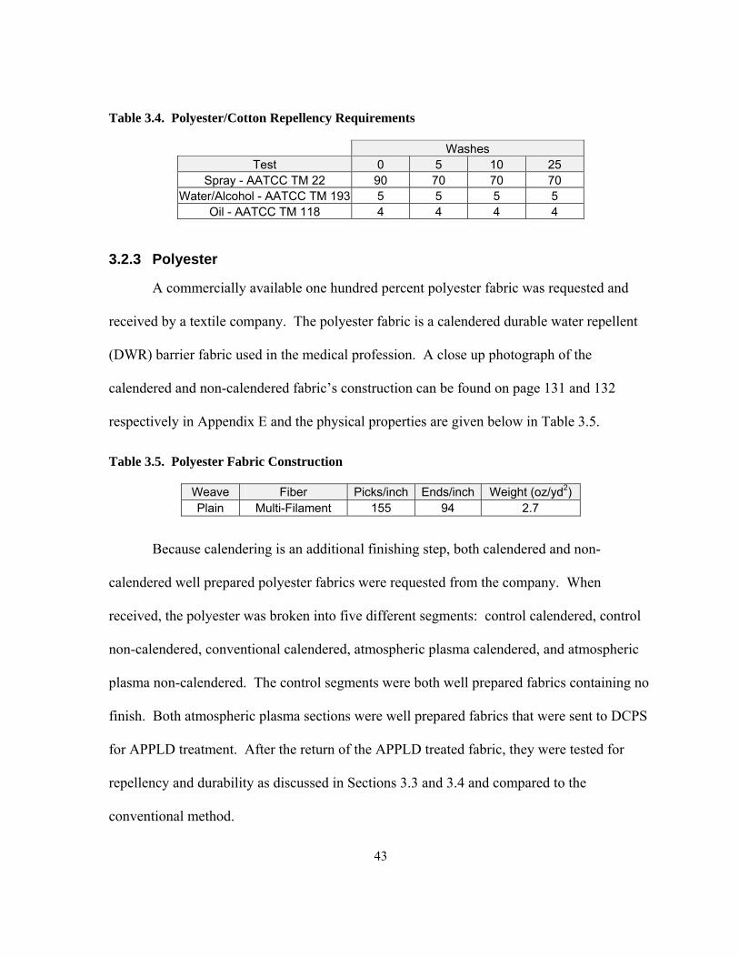
43
Table 3.4. Polyester/Cotton Repellency Requirements
Washes Test 0 5 10 25
Spray - AATCC TM 22 90 70 70 70 Water/Alcohol - AATCC TM 193 5 5 5 5
Oil - AATCC TM 118 4 4 4 4
3.2.3 Polyester
A commercially available one hundred percent polyester fabric was requested and
received by a textile company. The polyester fabric is a calendered durable water repellent
(DWR) barrier fabric used in the medical profession. A close up photograph of the
calendered and non-calendered fabric’s construction can be found on page 131 and 132
respectively in Appendix E and the physical properties are given below in Table 3.5.
Table 3.5. Polyester Fabric Construction
Weave Fiber Picks/inch Ends/inch Weight (oz/yd2) Plain Multi-Filament 155 94 2.7
Because calendering is an additional finishing step, both calendered and non-
calendered well prepared polyester fabrics were requested from the company. When
received, the polyester was broken into five different segments: control calendered, control
non-calendered, conventional calendered, atmospheric plasma calendered, and atmospheric
plasma non-calendered. The control segments were both well prepared fabrics containing no
finish. Both atmospheric plasma sections were well prepared fabrics that were sent to DCPS
for APPLD treatment. After the return of the APPLD treated fabric, they were tested for
repellency and durability as discussed in Sections 3.3 and 3.4 and compared to the
conventional method.

44
The only repellency test required by the company for this fabric is that it scores a 90
in the spray test before washing. Because this is a barrier fabric, additional physical tests
were performed as requested by the company. Table 3.6 below gives the performance
specification requirements of the calendered polyester.
Table 3.6. Polyester Additional Requirements
Test Measurement Hydrostatic Pressure – AATCC TM 127 55 cm minimum 5 Wash Shrinkage 3% length & width maximumAir Permeability – ASTM D737 2.5 cfm maximumTensile – ASTM D5034 120 lbs Warp & 70 lbs Fill minimum
The calendered sections were compared in order to determine the feasibility of the
company replacing their conventional finishing with the APPLD technology. The non-
calendered sections were analyzed, but were not compared to the calendered sections.
3.2.4 Nylon
A commercially available one hundred percent nylon fabric was requested and
received from a textile company. The fabric supplied was an apparel outerwear jacket
material that has a durable water repellent (DWR) finish. A close up photograph of the
fabric’s construction can be found on page 173 in Appendix F and the physical properties are
given below in Table 3.7.
Table 3.7. Nylon Fabric Construction
Weave Fiber Picks/in Ends/in Weight (oz/yd2) 3-Ply Multi-Filament 160 66 3.8

45
The company submitted a head end of their conventionally treated nylon fabric along
with prepared only fabric. The prepared only fabric received for treatment was well prepared
but not dyed. These fabrics received from the company were split into three segments:
control, conventional, and atmospheric plasma. The atmospheric plasma segment was a
section of the well prepared fabric that was sent to DCPS for APPLD treatment. After the
return of the APPLD treated fabric, it was tested for repellency and durability as discussed in
Sections 3.3 and 3.4 and compared to the conventional method. The repellency test
requirements provided by the company for this fabric is given below in Table 3.8.
Table 3.8. Nylon Repellency Requirements
Washes Test 0 5 10 25
Spray - AATCC TM 22 90 90 90 90
3.2.5 Nonwovens
Commercially available one hundred percent polyester and a one hundred percent
polypropylene nonwoven fabrics were submitted and received from a textile company. Both
nonwovens were being used in the automotive industry as water repellent products. They
were submitted for this research in an effort to try to find an alternative to the current
fluorocarbon aerosol application method. Both nonwovens were submitted to DCPS for
APPLD treatment but both were returned because they would not fit between the electrodes
for processing. Both nonwoven samples had a thickness of 4 mm. After DCPS returned the
samples, APJeT was contacted to treat the samples but our request was turned down because

46
we could not be scheduled within the next six months. For this reason, neither of the
nonwoven samples will be discussed for the remainder of this document.
3.3 Repellency Tests
A variety of tests were chosen in order to evaluate the repellency of each treated
fabric. The spray, impact, oil, and water/alcohol resistance tests are mostly subjective and
used most often in the textile industry to test how repellent a surface is to a liquid, while the
contact angle test is more objective and used in research. All of these tests were conducted in
accordance with the American Association of Textile Chemist and Colorists (AATCC)
standard test methods. For all tests performed, the fabrics were conditioned at 65 ± 2%
relative humidity and 70 ± 2 °F for a minimum of four hours before testing. Because the
polyester fabric received was a barrier fabric, additional tests were performed as discussed in
Section 3.3.6. All fabrics were conditioned in a temperature and humidity controlled room at
NCSU except for the impact and hydrostatic pressure test fabrics that were conditioned in the
AATCC’s Parameter Generation and Control conditioning chamber, model number 9134-
3119 in Research Triangle Park, NC.
3.3.1 Spray
The spray test is standardized as AATCC Test Method 22.32 This test was used to
measure the resistance of fabrics to wetting by water. The fabric samples were laid 150 mm
under a spray nozzle at a 45˚ angle and 250 mL of water was poured onto the fabric through
the spray nozzle. After the fabric was “smartly” tapped, and the wetting pattern was
compared with a standard rating chart given in Figure 3.1 on the following page. Complete

47
wetting resulted in a score of 0 while no wetting pattern received a score of 100. All spray
tests were conducted on spray test equipment as specified by the AATCC and were
performed at NCSU.
Figure 3.1. Spray Test Ratings

48
3.3.2 Impact
The impact penetration test, standardized as AATCC TM 4232, was used to simulate a
fabric’s exposure to rain. Unlike the spray test, this test method measures the resistance of
fabrics to the penetration of water by impact, thus it can be used to predict the resistance of
fabrics to rain penetration. For each sample, a weighed paper blotter was placed under the
fabric that was clamped on the top end at an angle of 45˚ and 500 mL of water was sprayed
onto the fabric 0.6 m below the nozzle. Immediately after spraying, the blotter paper was
reweighed and the difference in weight indicated penetration of water. All impact
penetration tests were conducted on a Type I tester as specified in the test method and were
performed at the AATCC lab in Research Triangle Park, NC.
3.3.3 Water/Alcohol
The water/alcohol test is known as the “Aqueous Liquid Repellency: Water/Alcohol
Solution Resistance Test” and is standardized as AATCC TM 193.32 This test was
performed to measure the repellency of each sample’s surface to wetting. This was
accomplished by placing aqueous solutions with decreasing surface tensions on each of the
fabric samples. There are eight different aqueous solutions in this test as seen in Table 3.9 on
the following page.

49
Table 3.9. AATCC TM 193 Standard Test Liquids
AATCC Aqueous Solution Repellency
Grade Number Composition (vol:vol) Surface
Tension *N
0 None (fails Grade 1) 1 98:2 / Water : isopropyl alcohol 59.0 2 95:5 / Water : isopropyl alcohol 50.0 3 90:10 / Water : isopropyl alcohol 42.0 4 80:20 / Water : isopropyl alcohol 33.0 5 70:30 / Water : isopropyl alcohol 27.5 6 60:40 / Water : isopropyl alcohol 25.4 7 50:50 / Water : isopropyl alcohol 24.5 8 40:60 / Water : isopropyl alcohol 24.0
*N = dynes/cm at 25°C
Five drops of the first solution, grade number 1, were placed on the fabric in different
locations along the filling direction approximately 4 cm apart. The drops were observed for
approximately 10 seconds from a 45° angle. After each aqueous solution was observed, it
was given a grade as shown in Figure 3.2.
Figure 3.2. AATCC TM 193 Solution Grades

50
If no penetration, wetting, or wicking occurred, the process was repeated for the next
solution’s aqueous grade number up to grade 8. If the three out of five solution drops of
grade 8 showed no sign of wetting or wicking and had a well-rounded drop, the fabric
received a grade of 8. If the grade was a borderline pass (a rating of B in Figure 3.2), the
grade was expressed to the nearest 0.5 value by subtracting one-half from the number of the
borderline test liquid. The best grade and therefore the highest repellency that can be
received by the water/alcohol test is an 8. All water/alcohol tests were performed at NCSU
using a ratio of 99.9% isopropyl alcohol to deionized water.
3.3.4 Oil
The oil test is also known as the “Oil Repellency Hydrocarbon Resistance Test” and
is standardized as AATCC TM 118.32 This test is the same as the water/alcohol test in every
way except for the test solutions used. The lowest liquid surface tension used in the
water/alcohol test is 24.0 dynes/cm but for the oil test it is 19.8 dynes/cm as shown in Table
3.10 on the following page.

51
Table 3.10. AATCC TM 118 Standard Test Liquids
AATCC Aqueous Solution Repellency
Grade Number Composition Surface
Tension *N
0 None (fails Grade 1) 1 Kaydol 31.5 2 65:35 Kaydol : n-hexadecane (vol:vol) 28.9 3 n-hexadecane 27.3 4 n-tetradecane 26.4 5 n-dodecane 24.7 6 n-decane 23.5 7 n-octane 21.4 8 n-heptane 19.8
*N = dynes/cm at 25°C
All oil tests were performed at NCSU using the chemicals listed above in Table 3.10.
All chemicals were at least 99.5% pure.
3.3.5 Contact Angle
Contact angle measurements were measured with a NCSU built microscopic
apparatus to view a water droplet on a surface. The microscope was positioned so that when
looking through it, the water droplet will appear similar to Figure 2.1.
The eyepiece contained a straight horizontal reference line that was placed between
the water droplet and the surface of the fabric and a second vertical line was adjusted to
represent the contact angle. When the reference and measurement lines were positioned as
shown in Figure 2.1 by the bold arrows, the contact angle θ was measured by the eyepiece’s
internal protractor. Each fabric finish was measured five times at different locations

52
throughout the roll. The contact angle measurements give an objective comparison of the
conventional and atmospheric plasma treatments.
3.3.6 Additional Tests
Because the polyester fabric received is a barrier fabric, the additional tests below
were performed.
3.3.6.1 Hydrostatic Pressure
The hydrostatic pressure test, standardized as AATCC TM 12732, was used to
measure the resistance of a fabric to the penetration of water under hydrostatic pressure. A
fabric sample was placed in a hydrostatic tester and the hydrostatic pressure was increased at
a constant rate. The pressure at which water penetrated through the fabric in three locations
was the penetration pressure and was measured in centimeters of water. All hydrostatic
pressure tests were performed at the AATCC lab in Research Triangle Park, NC.
3.3.6.2 Wash Shrinkage
The wash shrinkage test was performed by measuring and marking a ten inch by ten
inch square on six fabric samples from each finish. After five washes, as described in
Section 3.4.2, the squares were measured again. From knowing the dimensions of the box
before and after five washes, the percentage that the sample shrank was calculated in both the
warp and filling directions.

53
3.3.6.3 Air Permeability
Because the current facilities at NCSU do not have an air permeability machine that
can accurately calculate very low air flow due to a calendered product, the finished samples
were sent back to the company after treatment for internal testing. The results were shared
for this research.
3.3.6.4 Tensile
The tensile test performed on the polyester was the grab test standardized as ASTM D
503473. This test is also known as the “Standard Test Method for Breaking Strength and
Elongation of Textile Fabrics.” For this test, four inch wide by eight inch long fabric
specimens were mounted centrally in the clamps of a Sintech 1/S tensile testing machine at
NCSU. The clamps slowly separated until the fabric failed. Three samples were tested for
each finish in both the warp and filling directions. The Sintech testing machine is computer
controlled assuring that all settings adhere to the ASTM D 5034 procedure. The computer
calculated the breaking force in pounds and provided a printout for each finish tested.
3.4 Durability Tests
Durability testing was performed in order to determine if the atmospheric plasma
treatment can perform as well as conventional wet finishing after multiple launderings. The
repellency tests in Section 3.3 were performed at 0, 5, 10, and 25 washes. Each wash cycle
of 0, 5, 10 and 25 washes were mutually exclusive relative to repellency testing. For
example, a spray test was not performed at five washes and then again on the same sample at
10 washes; each test had a specific fabric sample for that test at a specific wash cycle only.

54
3.4.1 X-ray Photoelectron Spectroscopy
X-ray Photoelectron Spectroscopy (XPS) was used on all of the as received fabric
samples before any testing. XPS is a surface analysis technique used to determine the
concentration of different elements at the fabric surface. A more detailed explanation of XPS
can be found in Appendix B. The machine used in this research was a Riber LAS-3000 using
MgKα x-ray excitation. Energy calibration was established by referencing to the
adventitious carbon (C1s at 284.5 eV).
Using XPS analysis, an approximate amount of fluorine on the surface was
determined. This was necessary because it was possible that the atmospheric plasma
treatment could have placed a significantly higher or lower amount of fluorine on the surface
than the conventional treatment resulting in a bias. In order to determine if the durability
testing was biased, each finished fabric sample that was compared was tested by XPS in
order to determine if they had approximately the same percentage of fluorine on the surface.
Because each finish was applied to the same base fabric, the percentage of other elements
besides fluorine remained constant. Therefore, the percent of fluorine on the surface gave a
good indication of the actual amount of fluorine across each finish.
3.4.2 Wash
The washing procedure used adhered to AATCC TM 130 Section 8 and the
AATCC’s “Standardization of Home Laundry Test Conditions”. AATCC TM 130 Section 8
pertains to how the wash load is prepared and the latter for the settings used on the washer
and dryer. There were two small deviations away from AATCC 130 Section 8. The first

55
deviation was the sample size. The procedure calls for each sample to be washed to be 15
inches square. Because the fabric returned from DCPS was on a 12 inch reel, the sample size
was changed to be 12 by 15. Secondly, the procedure calls for no more than 30 specimens to
be placed in a washer although each fabric to be washed contained more than 30 specimens.
Table 3.11 below shows how many samples were needed for each fabric in order to complete
the tests in Section 3.3 for each wash cycle. Because of the large number of fabric samples,
the 30 specimen limit per wash was ignored. For each wash, more than 30 specimens were
loaded into the washer.
Table 3.11. Number of Samples Required for Each Fabric
Fabric SamplesPolyester 120 Nylon 48 Cotton 32 Polyester/Cotton 64
Because of the amount of samples that were to be washed, they were split up between
two washers and dryers. All samples washed in washer A were dried in dryer A and samples
washed in washer B were dried in dryer B. The equipment used is given in Table 3.12
below.
Table 3.12. Wash Equipment
Make Model Washer A Kenmore 110.26712693 Washer B Kenmore 92596100 Dryer A Kenmore 110.6493220 Dryer B Kenmore 110.60932990

56
The nylon and polyester samples were washed in washer A while the cotton and
polyester/cotton samples were washed in washer B. Thirty six inch square 100 percent
polyester ballasts were added to the nylon and polyester set while 36 inch square 100 percent
cotton ballasts were added to the cotton and polyester/cotton set to reach 4.0 lbs of fabric to
be washed in each machine. One hundred grams of AATCC 1993 Standard Reference
Detergent was added to each wash load. The detergent was measured on a scale to within
one tenth of a gram. The washing machine settings for both the nylon-polyester and the
cotton-polyester/cotton sets are given in Table 3.13 below.
Table 3.13. Washing Machine Settings
Wash Temp Rinse Temp Cycle Wash Time Warm: 105 ± 5°F < 85 °F Normal 10 min
After a load of fabric samples were washed, they were immediately placed in the
dryer. The machine settings for the dryer are given in Table 3.14 below.
Table 3.14. Dryer Machine Settings
Technique Cycle Dry Time Tumble Normal 45 min
After five washes, the samples labeled for testing at five washes as described in
Section 3.4 were removed. More ballast was added to get the next wash load up to 4.0
pounds and the process was repeated. After ten washes the samples marked for testing at ten
washes were removed leaving only the samples for testing at twenty five washes.

57
By comparing the results of the repellency tests discussed in Section 3.3 for 0, 5, 10,
and 25 washes, a comparison of durability to washing between a conventional and
atmospheric plasma treatment was made.
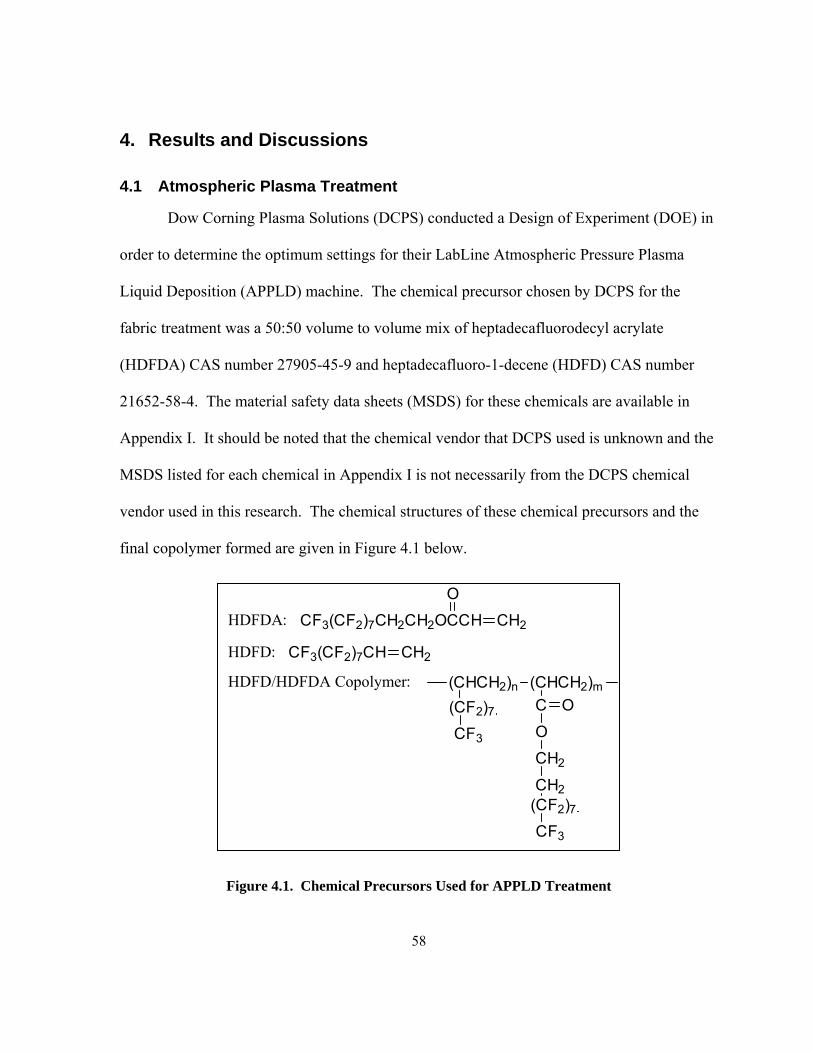
58
4. Results and Discussions
4.1 Atmospheric Plasma Treatment
Dow Corning Plasma Solutions (DCPS) conducted a Design of Experiment (DOE) in
order to determine the optimum settings for their LabLine Atmospheric Pressure Plasma
Liquid Deposition (APPLD) machine. The chemical precursor chosen by DCPS for the
fabric treatment was a 50:50 volume to volume mix of heptadecafluorodecyl acrylate
(HDFDA) CAS number 27905-45-9 and heptadecafluoro-1-decene (HDFD) CAS number
21652-58-4. The material safety data sheets (MSDS) for these chemicals are available in
Appendix I. It should be noted that the chemical vendor that DCPS used is unknown and the
MSDS listed for each chemical in Appendix I is not necessarily from the DCPS chemical
vendor used in this research. The chemical structures of these chemical precursors and the
final copolymer formed are given in Figure 4.1 below.
C F 3 ( CF2)7CH CH2HDFD :
C F 3(CF2)7CH2CH2OCCHO
CH2HDFDA :
(CHCH2)n (CHCH 2 ) m (CF2)7CF3
C O
OCH2
CH2(CF2)7 CF3
HDFD/HDFDA Copolymer:
Figure 4.1. Chemical Precursors Used for APPLD Treatment

59
The DOE performed by DCPS is given below in Table 4.1.
Table 4.1. DCPS APPLD DOE Operating Conditions
Run 1 2 3 4 5 6 7 8 Line Speed
(m/min) 5 10 5 10 5 10 10 5
Precursor Flow Rate (μl/min) 1000 1500 1500 1000 1000 1000 1500 1500
Power (W) 1800 1800 2000 1800 2000 2000 2000 1800
Number of Passes 1 1 1 3 3 1 3 3
The machine settings found by DCPS to be optimum for repellency were determined
to be the settings used at run number eight. These settings along with the constant settings
used for each run is given below in Table 4.2.
Table 4.2. DCPS LabLine Machine Settings
Optimal Parameters Constant Settings Precursor Flow Rate 1.5 mL/min Gas Helium Power 1.8 kW Gas pressure to nozzle 50 psi Line Speed 5 m/min Gas flow rate to top box 10 L/min Passes 3 Gas flow rate to shower seals 15 L/min
Twenty meters of APPLD treated fabric were returned for each fabric sent with the
exception of both nonwoven samples. They were not analyzed or treated because with a
thickness of 4mm, they were “too thick” to pass through the LabLine’s electrode gap.
Upon inspection of the returned fabrics, they all contained tiny holes on a significant
area of the twenty meters returned. When referring back to the accompanying report, DCPS
stated the following:
“All fabric substrates were seen to exhibit some micro-discharges during the plasma treatment, as a result, pinholes were observed in
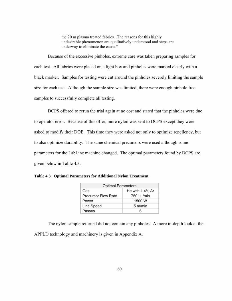
60
the 20 m plasma treated fabrics. The reasons for this highly undesirable phenomenon are qualitatively understood and steps are underway to eliminate the cause.”
Because of the excessive pinholes, extreme care was taken preparing samples for
each test. All fabrics were placed on a light box and pinholes were marked clearly with a
black marker. Samples for testing were cut around the pinholes severely limiting the sample
size for each test. Although the sample size was limited, there were enough pinhole free
samples to successfully complete all testing.
DCPS offered to rerun the trial again at no cost and stated that the pinholes were due
to operator error. Because of this offer, more nylon was sent to DCPS except they were
asked to modify their DOE. This time they were asked not only to optimize repellency, but
to also optimize durability. The same chemical precursors were used although some
parameters for the LabLine machine changed. The optimal parameters found by DCPS are
given below in Table 4.3.
Table 4.3. Optimal Parameters for Additional Nylon Treatment
Optimal Parameters Gas He with 1.4% Ar Precursor Flow Rate 750 μL/min Power 1500 W Line Speed 5 m/min Passes 6
The nylon sample returned did not contain any pinholes. A more in-depth look at the
APPLD technology and machinery is given in Appendix A.

61
4.2 Repellency & Durability
Repellency tests discussed in Section 3.3 were performed at each wash cycle of 0, 5,
10, and 25 as discussed in Section 3.4. All graphs and statistical conclusions were produced
and calculated by JMP® 6 statistical software available by SAS© at www.jmp.com. Results
are considered to be statistically significant if p-values are less than 0.05. Data collected in
this research is assumed to be of the normal distribution.
4.2.1 Cotton
The cotton fabric contained three segments: control, conventional, and atmospheric
plasma as discussed in Section 3.2.1. The nomenclature used throughout the remainder of
the document is given in Table 4.4 on the following page. Tabular results of all cotton as
received repellency tests along with tests at 5 and 10 washes can be found on page 117 in
Appendix C.
Table 4.4. Cotton Fabric Nomenclature
Abbreviation Segment Description CTRL control cotton fabric with no finish (prepared only)
W conventional cotton fabric with conventional wet pad-dry-cure finish P atmospheric plasma cotton fabric treated with APPLD
4.2.1.1 XPS Analysis
An XPS analysis was performed as discussed in Section 3.4.1 on all three cotton
segments. Table 4.5 shows the percent fluorine composition of each segment. The complete
elemental composition can be found on page 117 in Appendix C.

62
Table 4.5. Fluorine Composition of Cotton Segments
Segment CompositionCTRL 0%
W 62% P 63%
As expected, the CTRL segment does not have a repellent finish, therefore no
fluorine was detected on the surface with only carbon and oxygen present from the cotton
molecules. For both the W and P finishes, fluorine was found to represent 62 and 63 percent
of the surface respectively. Also, the binding energies for both the W and P finish are
extremely similar, given on page 116, suggesting that both the W and P finishes have not
only the same amount of fluorine on the surface, but both surfaces have an analogous
chemical composition. Therefore, it can be expected that no initial bias in repellency or
durability exists between the W or P finishes.
4.2.1.2 Spray
Spray tests were preformed as discussed in Section 3.3.1 on all as received samples
along with samples washed 5 and 10 times. The results of the spray test shown in Table 4.6
are the score as given by Figure 3.1 on page 47. The average of two tests was used to
determine the results. The results for each individual test can be found on page 117 in
Appendix C.
Table 4.6. Cotton Spray Results
Washes Finish 0 5 10
W 100 95 88 P 100 55 0

63
The CTRL segment is not included in the results of Table 4.6 because it scored a 0.
For this reason, the CTRL segment will not be included in any of the proceeding tests
discussed in this section. In addition, at 10 washes, the P finish sample was completely
saturated by the water from the spray test also resulting in a score of 0. Therefore, the cotton
was not tested at 25 washes for this or any other proceeding test. After 5 washes, as shown
in Table 4.6, the P finish showed a dramatic drop in repellency relative to the W finish.
4.2.1.3 Impact
Impact tests were performed as discussed in Section 3.3.2 on all as received samples
along with samples washed 5 and 10 times. The results of the test shown below in Table 4.7
are in grams (g) of water penetrated through the fabric. The average of three tests was used
to calculate the results. In accordance with AATCC TM 42, if more than five grams of water
penetrates through the fabric, it is recorded as “>5 g”. Results for each individual test can be
found on page 117 in Appendix C.
Table 4.7. Cotton Impact Penetration Results
Washes Finish 0 5 10
W 1.2 g 0.1 g 0.0 g P 0.4 g > 5 g > 5 g
Table 4.7 shows that the P finish initially outperformed the W finish. Although this is
true for the samples before washing, the W finish improved slightly through ten washes
while the P finish failed after just five. The W finish performance is most likely due to the
fabric shrinking and therefore decreasing the capillary pores of the fabric surface. With a

64
tighter construction of the fabric in addition to the repellent finish still left on the surface, the
amount of water that penetrated through the W finish decreased after 5 and 10 washes. The P
finish also had some shrinkage observed after 5 and 10 washes, but by the results of the spray
test, most of the repellent finish was removed after 5 washes.
4.2.1.4 Water/Alcohol
Water/alcohol tests were performed as discussed in Section 3.3.3 before washing
along with samples washed 5 and 10 times. The results of the water/alcohol test shown in
Table 4.8 on the following page were determined by Table 3.9 and Figure 3.2 as described in
Section 3.3.3.
Table 4.8. Cotton Water/Alcohol Results
Washes Finish 0 5 10
W 7.5 8 8 P 7.5 0.5 0
Table 4.8 shows that both the W and P finishes are comparable before washing.
Although the W finish slightly improved through 5 and 10 washes, the P finish showed a
dramatic decrease in repellency after just 5 and 10 washes.
4.2.1.5 Oil
Oil tests were performed as discussed in Section 3.3.4 on all as received samples
along with samples washed 5 and 10 times. The results of the oil test shown in Table 4.9
were determined by Table 3.10 and Figure 3.2 as described in Section 3.3.4.

65
Table 4.9. Cotton Oil Results
Washes Finish 0 5 10
W 6.5 6 6 P 6.5 5 2
Table 4.9 shows that both the W and P finishes are comparable before washing. The
W finish is consistent around a grade of 6 although the P finish shows a significant decrease
in repellency after 10 washes down to a grade of 2 from 6.5.
4.2.1.6 Water Contact Angle
Contact angle measurements were taken as discussed in Section 3.3.5 for all as
received samples along with samples washed 5 and 10 times. The results of the contact angle
tests shown in Table 4.10 are the average of five different measurements and are given in
degrees. The results for each individual test can be found on page 117 in Appendix C.
Table 4.10. Cotton Contact Angle Results
Washes Finish 0 5 10
W 157° 145° 143° P 152° 0° 0°
Analysis of Variance (ANOVA) tests in Appendix C were conducted on the data used
to generate Table 4.10 in order to compare the repellency and durability of the finishes. An
ANOVA was conducted between and within each finish. When testing the P finish samples
at 5 and 10 washes, no measurement could be taken because by the time the apparatus was
adjusted and ready for measurement, the water had absorbed into the fabric resulting in a
contact angle of 0°.

66
The ANOVA between finishes determines if there is a statistically significant
difference in the water contact angle between each finish at each wash cycle. In this case,
only the as received samples could be compared. The results of this ANOVA on page 118
in Appendix C shows that with the given data, there is no statistical difference in the water
contact angle between the W and P finishes before washing.
The ANOVA within each finish determines the statistical significance of how much,
or even if, each specific repellent finish deteriorates after each wash cycle. In this case, only
the W finish could be analyzed. The results of this ANOVA on page 119 in Appendix C
shows that the water contact angle drops by about 10° after 5 washes for the W finish. Also,
there is no statistical difference between 5 and 10 washes.
4.2.2 Polyester/Cotton
The polyester/cotton fabric contained four segments: control, conventional, member
conventional, and atmospheric plasma as discussed in Section 3.2.2. As discussed on page
42, the member conventional segment had a limited amount of fabric for testing. Because of
the pinholes as discussed on page 59, the amount of fabric for the atmospheric plasma
segment was also limited. Therefore, both the member conventional and conventional
segments could be compared to the atmospheric plasma segment. The nomenclature used
throughout the remainder of the document is given in Table 4.11 on the following page.

67
Table 4.11. Polyester/Cotton Fabric Nomenclature
Abbreviation Segment Description
CTRL control polyester/cotton fabric with no finish (prepared only)
W conventional polyester/cotton fabric with conventional wet pad-dry-cure finish
WM member conventional commercially available polyester/cotton fabric with conventional finish
P atmospheric plasma polyester/cotton fabric with APPLD
4.2.2.1 XPS Analysis
An XPS analysis was performed as discussed in 3.4.1 on all four polyester/cotton
segments. Table 4.12 shows the percent fluorine composition of each segment. The full
elemental compositions can be found on page 122 in Appendix D.
Table 4.12. Fluorine Composition of Polyester/Cotton Segments
Segment CompositionCTRL 0%
W 65% WM 60%
P 64%
As expected, the CTRL segment does not have a repellent finish therefore no fluorine
was detected on the surface. For both the W and P finishes, the fluorine was found to
represent 65 and 64 percent of the surface respectively. The WM finish contained slightly
less fluorine as a percentage on the surface because of a small presence of nitrogen. The
presence of nitrogen was most likely contamination due to the soil release finish on the
opposite side of the fabric. Also, the binding energies for the W, WM, and P finishes, shown
on page 121, are all extremely similar suggesting that all three finishes have the same amount

68
of fluorine on the surface and both surfaces have an analogous chemical composition.
Therefore, it can be expected that there is no initial bias in repellency or durability among the
W, WM, or P finishes.
4.2.2.2 Spray
Spray tests were performed as discussed in Section 3.3.1 on all as received samples
along with samples washed 5, 10, and 25 times. The results of the spray test shown in Table
4.13 are the scores as given by Figure 3.1 on page 47. The average of three tests was used to
determine the results. The results for each individual test can be found on page 122 in
Appendix D.
Table 4.13. Polyester/Cotton Spray Results
Washes Finish 0 5 10 25
W 100 100 100 98 WM 100 100 98 92
P 97 80 70 53
The CTRL segment is not included in the results of Table 4.13 because it scored a 0.
For this reason, the CTRL segment will not be included in any of the proceeding tests
discussed in this section. As shown in Table 4.13, the W and WM conventional finishes
score quite well at 5, 10, and even 25 washes while the P finish slowly decreased in
repellency at each wash cycle. Referring back to Table 3.4, the P-finish fails the company’s
requirement of a minimum spray score of 70 at 25 washes.

69
4.2.2.3 Impact
Impact tests were performed as discussed in Section 3.3.2 on all as received samples
along with samples washed 5, 10, and 25 times. The results of the tests are shown below in
Table 4.14 in grams (g) of water penetrated through the fabric. The average of three tests
was used to calculate the results. In accordance with AATCC TM 42, if more than five
grams of water penetrates through the fabric, it is recorded as “>5g”. The results for each
individual test can be found on page 122 in Appendix D.
Table 4.14. Polyester/Cotton Impact Penetration Results
Washes Finish 0 5 10 25
W > 5 g 3.6 g 3.5 g 1.4 g WM > 5 g > 5 g 4.7 g 3.9 g
P > 5 g > 5 g > 5 g > 5 g
Table 4.14 shows that all finishes absorbed more than 5 grams of water before
washing. After washing, the W finish was dramatically improved after 25 washes while the
WM finish improved after 5 and 10 washes but deteriorated after 25. The P finish absorbed
more than 5 grams of water for each wash cycle. It should be noted that the P finish allowed
over 15 grams of water to penetrate the fabric for nearly every test. A fully saturated paper
blotter varied in weight between 16 and 18 grams. This suggests that the P finish had a
minimal protection of impact resistance. This may be because the polymerized water
repellent film failed allowing water to pass easily into the bulk of the fabric.
The interesting results observed between the W and WC finishes can be explained by
both the fabric’s construction and the durability of the repellent finish after each wash cycle.

70
The polyester/cotton fabric tested in this research was very porous as shown on page 120.
Because the fabric contained large capillary spaces within the fabric, it was expected that it
would not perform well in the impact test. After each wash cycle, the fabric shrank
decreasing the pore size. This can explain the improved performance over each wash cycle
for both the W and WM finishes. The spray test suggested that the W finish is more repellent
than the WM finish after 10 and 25 washes. This can help explain how the W finish allowed
less water to penetrate the fabric than the WC finish.
4.2.2.4 Water/Alcohol
Water/alcohol tests were performed as discussed in Section 3.3.3 on all as received
samples along with samples washed 5, 10, and 25 times. The results of the water/alcohol
tests shown in Table 4.15 were determined by Table 3.9 and Figure 3.2 as described in
Section 3.3.3.
Table 4.15. Polyester/Cotton Water/Alcohol Results
Washes Finish 0 5 10 25
W 8 8 8 8 WM 8 8 8 6.5
P 8 6.5 5.5 3
Table 4.15 shows that all unwashed finishes received the highest grade of 8. Both
conventional W and WM finishes are comparable with WM having a small decrease in
repellency after 25 washes. The P finish’s repellency slowly decreased as washes increased
down to a grade of 3 after 25 washes. Referring back to Table 3.4, the P finish fails the
company’s requirement of a minimum grade of 5 at 25 washes.

71
4.2.2.5 Oil
Oil tests were performed as discussed in Section 3.3.4 on all as received samples
along with samples washed 5, 10, and 25 times. The results of the oil test shown in Table
4.16 were determined by Table 3.10 and Figure 3.2 as described in Section 3.3.4.
Table 4.16. Polyester/Cotton Oil Results
Washes Finish 0 5 10 25
W 6.5 6.5 6.5 6.5 WM 7.5 6.5 6.5 6.5
P 7.5 6.5 5.5 5
Table 4.16 shows that each finish is comparable before washing. Both conventional
finishes remained mostly constant through 25 washes although the P finish decreases slowly
in repellency after each wash cycle. Referring back to Table 3.4, the P finish just passes the
company’s requirement of a minimum grade of 5 after 25 washes.
4.2.2.6 Water Contact Angle
Contact angle measurements were taken as discussed in Section 3.3.5 for all as
received samples along with samples washed 5, 10, and 25 times. The results of the contact
angle tests shown in Table 4.17 on the following page are the average of five different
measurements and are given in degrees. The results for each individual water contact angle
test can be found on page 123 in Appendix D.

72
Table 4.17. Polyester/Cotton Contact Angle Results
Washes Finish 0 5 10 25
W 150° 155° 153° 151° WM 156° 155° 154° 152°
P 150° 146° 142° 138°
Analysis of Variance (ANOVA) tests in Appendix D were conducted on the data used
to generate Table 4.17 in order to compare the repellency and durability of the finishes. An
ANOVA was conducted both between and within each finish.
The ANOVA between finishes determines if there is a statistically significant
difference in water contact angles between each finish at each wash cycle. The results of
these ANOVAs on pages 124 through 127 show that before washing there is no difference
between the W and P finishes although there is a borderline statistical significance of the
WM finish having a water contact angle approximately 5 degrees greater then the W and P
finishes. At 5 washes the conventional W and WM finishes had a statistically higher water
contact angle by 5 degrees over the P finish. This is also true at 10 and 25 washes except the
angle increased from 5 degrees to 10 and 12 degrees respectively.
The ANOVA within each finish determines the statistical significance of how much,
or even if, each specific repellent finish deteriorates after each wash cycle. The results of
these ANOVAs on pages 128 though 130 show that from the data collected, no significant
difference in repellency can be determined for the conventional finishes, although a
difference is observed for the P finish. The P finish shows a slow descending progression in

73
the water contact angle where there is a statistical difference in the contact angle between 0
and 25 washes by about 12°.
4.2.3 Polyester
The polyester fabric contained five segments: control calendered, control non-
calendered, conventional calendered, atmospheric plasma calendered, and atmospheric
plasma non-calendered as discussed in Section 3.2.3. The nomenclature used throughout the
remainder of the document is given below in Table 4.18.
Table 4.18. Polyester Fabric Nomenclature
Abbreviation Segment Description
C-CTRL control calendered calendered PET with no finish (prepared only)
NC-CTRL control non-calendered non-calendered PET with no finish (prepared only)
C-W conventional calendered commercially available calendered PET with conventional finish
C-P atmospheric plasma calendered calendered PET with APPLD finish
NC-P atmospheric plasma non-calendered non-calendered PET with APPLD finish
4.2.3.1 XPS Analysis
An XPS analysis was performed as discussed in 3.4.1 on all five polyester segments.
Table 4.19 on the following page shows the percent fluorine composition of each nylon
segment. The full elemental compositions can be found on page 134 in Appendix E.

74
Table 4.19. Fluorine Composition of Polyester Segments
Segment Composition C-CTRL 0%
NC-CTRL 0% C-W 63% C-P 64%
NC-P 65%
As expected, the CTRL segments do not have a repellent finish therefore no fluorine
was detected on the surface. For the C-W, C-P, and NC-P finishes, fluorine was found to
represent 63, 64, and 65 percent of the surface respectively. Also, the binding energies for
the C-W, C-P, and NC-P finishes are all extremely similar suggesting that all three finishes
have the same amount of fluorine on the surface and all of the surfaces have an analogous
chemical composition. Therefore, it can be expected that there is no initial bias in repellency
or durability between the C-W, C-P, or the NC-P finish. The full scan of each polyester
segment can be found on page 133 in Appendix E.
4.2.3.2 Spray
Spray tests were performed as discussed in Section 3.3.1 on all as received samples
along with samples washed 5, 10, and 25 times. The results of the spray test shown in Table
4.20 on the following page are the score as given by Figure 3.1 on page 47. The average of
three tests was used to determine the results. The results for each individual test can be
found on page 134 in Appendix E.

75
Table 4.20. Polyester Spray Results
Washes Finish 0 5 10 25 C-W 100 100 100 100 C-P 100 100 100 100
NC-P 100 100 100 100
Neither of the CTRL segments are included in the results of Table 4.20 because they
both scored a 0. For this reason, the CTRL segments will not be included in any of the
proceeding tests discussed in this section. Table 4.20 shows that all three finishes scored a
perfect score of 100 before and after each wash cycle. Referring back to page 44, all finishes
pass the companies’ requirement for an as received score of at least 90.
4.2.3.3 Impact
Impact tests were performed as discussed in Section 3.3.2 on all as received samples
along with samples washed 5, 10, and 25 times. The results shown below in Table 4.21 are
in grams (g) of water penetrated through the fabric. The average of three tests was used to
calculate the results. The results for each individual test can be found on page 134 in
Appendix E.
Table 4.21. Polyester Impact Penetration Results
Washes Finish 0 5 10 25 C-W 0g 0g 0g 0g C-P 0g 0g 0g 0g
NC-P 0.1g 0.1g 0.1g 0.1g
Table 4.21 shows that the conventional C-W finish and the C-P finish allowed no
penetration of water through the fabric. The NC-P finish also performed well allowing only

76
a slight penetration of water through the fabric most likely due to the non-calendered fabric
having larger capillary spaces than the calendered fabrics.
4.2.3.4 Water/Alcohol
Water/alcohol tests were performed as discussed in 3.3.3 on all as received samples
along with samples washed 5, 10, and 25 times. The results of the water/alcohol test shown
in Table 4.22 were determined by Table 3.9 and Figure 3.2 as described in Section 3.3.3.
Table 4.22. Polyester Water/Alcohol Results
Washes Finish 0 5 10 25 C-W 7.5 7.5 6.5 6.5 C-P 8 8 8 8
NC-P 8 8 8 8
Table 4.22 shows that both the C-P and NC-P atmospheric plasma finishes scored the
highest score possible in the water/alcohol test both before and after each wash cycle. The
conventional C-W also performed well, but showed a slight decrease in repellency after 10
washes.
4.2.3.5 Oil
Oil tests were performed as discussed in Section 3.3.4 on all as received samples
along with samples washed 5, 10, and 25 times. The results of the oil tests shown in Table
4.23 on the following page were determined by Table 3.10 and Figure 3.2 as described in
3.3.4.

77
Table 4.23. Polyester Oil Results
Washes Finish 0 5 10 25 C-W 4.5 4 3 2 C-P 5.5 5 5 5.5
NC-P 5 5.5 5.5 5.5
Table 4.23 shows that the conventional C-W finish decreases in repellency after each
wash cycle while the atmospheric plasma finishes C-P and NC-P do not. The results of the
oil tests suggest that the atmospheric plasma finish is more repellent and more durable than
the conventional finish.
4.2.3.6 Water Contact Angle
Contact angle measurements were taken as discussed in Section 3.3.5 for all as
received samples along with samples washed 5, 10, and 25 times. The result of the contact
angle tests shown in Table 4.24 are the average of five different measurements and are given
in degrees. The results of each individual water contact angle test can be found on page 135
in Appendix E.
Table 4.24. Polyester Contact Angle Results
Washes Finish 0 5 10 25 C-W 131° 143° 144° 145° C-P 127° 142° 146° 145°
NC-P 155° 151° 153° 154°
Analysis of Variance (ANOVA) tests in Appendix E were conducted on the data used
to generate Table 4.24 in order to compare the repellency and durability of the finishes. An
ANOVA was conducted both between and within each finish.

78
The ANOVA between finishes determines if there is a statistically significant
difference in water contact angles between each finish at each wash cycle. The results of
these ANOVAs on pages 138 through 141 show that for each wash cycle the non-calendered
NC-P finish had a statistically greater contact angle than the calendered C-W and C-P
finishes. This is most likely explained by the non-calendered fabric having a slightly rougher
surface than the calendered fabrics. Although the NC-P finish had a greater contact angle
then the other finishes, the ANOVA shows that the C-W and C-P finishes do not have
statistically different water contact angles.
The ANOVA within each finish determines the statistical significance of how much,
or even if, each specific repellent finish deteriorates after each wash cycle. The results of
these ANOVAs on pages 142 though 144 show that for both calendered finishes C-W and C-
P, the contact angle before washing was lower then the angles measured after washing by
about 12°. This is most likely because of the smooth surface of the calendered fabric. After
washing the C-W and C-P finishes, the contact angles increased because the washing caused
the surface to become slightly rougher. At 5, 10, and 25 wash cycles, the C-W and C-P
finishes did not have a statistically different water contact angle. The NC-P finish does not
have a statistically different water contact angle at 0, 5, 10 or 25 washes.
4.2.3.7 Additional Tests
The polyester fabric is a barrier fabric; therefore, additional tests were performed to
ensure that the atmospheric plasma treatment would not negatively affect the physical
properties of the fabric. Because calendering changes the physical properties of the fabric,

79
the non-calendered NC-P finish was not compared to the calendered C-W and C-P finishes.
The non-calendered finish results are provided to show the effects of atmospheric plasma
treatment on non-calendered fabrics for academic purposes only.
Hydrostatic Pressure Test
The hydrostatic pressure test was performed as described in Section 3.3.6.1 for all as
received samples along with samples washed 5, 10, and 25 times. The results, shown below
in Table 4.25, are in centimeters (cm) of water. The higher the water reaches in centimeters,
the greater the pressure on the fabric before failure. The average of three tests was used to
calculate the results. The results for each individual test can be found on page 136 in
Appendix E.
Table 4.25. Polyester Hydrostatic Pressure Results
Washes Finish 0 5 10 25 C-W 67cm 80cm 71cm 67cm C-P 96cm 80cm 76cm 71cm
NC-P 42cm 41cm 42cm 43cm
As expected, Table 4.25 shows that the non-calendered finishes tend to fail at lower
pressures than the calendered finishes. An ANOVA between finishes given on pages 145
through 148 shows that at 0 and 10 washes there is a statistical difference between the
conventional C-W and atmospheric plasma C-P calendered finishes. Before washing, the C-
P finish can withstand a greater pressure than the C-W finish by about 25 cm but only by a
few cm after 10 washes.

80
An ANOVA within finishes given on pages 149 through 151 shows that for the
conventional C-W finish, there is no statistical difference between failure at 0, 10, and 25
washes but the pressure to fail at 5 washes was statistically higher by more than 5 cm. The
ANOVA also shows a steady decrease in the pressure needed to fail the C-P finish resulting
in a statistical difference between 0 and 5 washes, and then again between 5 and 25 washes.
There was no significant statistical difference found in the height of water needed to fail the
fabric for the non-calendered NC-P finish. Referring back to Table 3.6, both the
conventional C-W and the atmospheric plasma C-P finish are well within 55 cm minimum
specification of the product.
Wash Shrinkage
The wash shrinkage test was performed on samples that had been washed 5 times as
described in Sections 3.3.6.2 and 3.4.2. The results, shown below in Table 4.26, are in
percent of shrinkage. An average of six samples was used to calculate the results. The
results for each individual test can be found on page 136 in Appendix E.
Table 4.26. Polyester 5 Wash Shrinkage Results
Direction Finish Warp Fill
C-CTRL 1.5% 0.3% NC-CTRL 1.5% 0.3%
C-W 0.7% 0.1% C-P 2.1% 0.6%
NC-P 3.9% 0.1%
Table 4.26 shows that the conventional C-W finish does not shrink after five washes
as much as the atmospheric plasma C-P finishes. This can be explained because the C-W

81
finish has already been exposed to heat during the pad-dry-cure process. The C-P finish was
first subjected to heat during laundering and therefore shrank more than the C-P finish after 5
washes. Referring back to Table 3.6, both the conventional C-W and the atmospheric plasma
C-P finishes were well within the 3% shrinkage specification of the product.
Air Permeability
Air permeability testing was performed by the company that submitted the fabric as
discussed in Section 3.3.6.3 for all as received samples along with samples washed 5, 10, and
25 times. The results shown in Table 4.27 are in cubic feet per minute (cfm). The results for
each individual test can be found on page 136 in Appendix E.
Table 4.27. Polyester Air Permeability Results
Washes Finish 0 5 10 25 C-W 0.7cfm 0.7 cfm 0.8 cfm 0.8 cfm C-P 0.3 cfm 0.4 cfm 0.9 cfm 1.0 cfm
NC-P 7.9 cfm 10.2 cfm 9.8 cfm 10.0 cfm * C-CTRL = 0.4 cfm, NC-CTRL = 9.4 cfm
As expected, Table 4.27 shows that the non-calendered finish allows more air through
the fabric than the calendered finishes. ANOVAs performed between the C-W and C-P
finishes on pages 152 through 155 shows that each cfm difference given in Table 4.27 is
statistically significant. The C-P finish initially allowed less air to pass through it although
at 10 washes the performance of the C-W finish overcomes it. This could possibly be
explained by the C-P finish having an additional polymerized thin film that contributed to
preventing air from passing though the fabric, but after 25 washes, the film was not as

82
effective. This hypothesis is backed up by the ANOVA within the C-P finish discussed in
the following paragraph.
ANOVAs were also performed within the C-W and C-P finish to determine if the air
permeability was affected by washing for each finish. These ANOVAs on pages 156 through
158 show that the C-W finish was very consistent through each wash cycle although the C-P
finish was not. For each wash cycle, the amount of air passed through the C-P finish became
greater and greater. The NC-P finish showed a large increase in air permeability after
washing. The NC-P wash results of 5, 10, and 25 washes were not statistically different.
Referring back to Table 3.6, both the conventional C-W and the atmospheric plasma C-P
finish are well within the 2.5 cfm maximum specification of the product.
Tensile
The tensile tests were performed as described in Section 3.3.6.4 for all as received
samples along with samples washed 5, 10, and 25 times. The results shown on the following
page in Table 4.28 and Table 4.29 are in pounds (lb) of breaking force in the warp and filling
direction respectively. The average of five tests was used to calculate the results. The results
for each individual test can be found on page 137 in Appendix E.

83
Table 4.28. Polyester Tensile Test Results in the Warp Direction
Washes Finish 0 5 10 25 C-W 177 lb 175 lb 175 lb 170 lb C-P 169 lb 173 lb 175 lb 173 lb
NC-P 177 lb 171 lb 175 lb 170 lb * C-CTRL = 184 lb, NC-CTRL = 181 lb
ANOVAs on pages 159 through 162 were conducted on the data used to generate
Table 4.28 to determine if there is a statistical difference in breaking strength in the warp
direction between the finishes across each wash cycle. It suggests that the C-W finish has a
higher breaking strength than the C-P finish by about 7 pounds although there is no statistical
difference in warp breaking strength between the two finishes after 5 or more washes.
ANOVAs were also conducted within each finish on pages 163 through 165 and found there
to be no statistical difference between washes within each finish. Referring back to Table
3.6, the warp breaking strength is well above the 120 pound minimum for each finish.
Table 4.29. Polyester Tensile Test Results in the Fill Direction
Washes Finish 0 5 10 25 C-W 100 lb 90 lb 100 lb 104 lb C-P 107 lb 103 lb 107 lb 99 lb
NC-P 108 lb 110 lb 108 lb 108 lb * C-CTRL = 104 lb, NC-CTRL = 108 lb
ANOVAs on pages 166 through 169 were conducted on the data used to generate
Table 4.29 to determine if there is a statistical difference in breaking strength in the fill
direction between the finishes across each wash cycle. The ANOVA shows that for 0, 5, and
10 washes, the C-P finish has a higher breaking strength than the C-W finish by about 7, 13,

84
and 7 pounds respectively. After 25 washes, the breaking strength of the C-W finish is
slightly greater than the C-P finish by 5 pounds.
ANOVAs were also conducted on pages 170 through 172 within each finish to
determine if each finish’s breaking strength changed after each wash cycle. The ANOVA
shows no statistical difference in the breaking strength in the filling direction of the NC-P
finish, but it does show a statistical difference in both the conventional C-W and atmospheric
plasma C-P finish. The conventional C-W finish had a lower breaking strength at 5 washes
than it did at 0, 10, and 25 washes by about 10 pounds. The atmospheric plasma C-P finish
had a lower breaking strength at 25 washes than at 0 and 10 washes by about 5 pounds.
Referring back to Table 3.6, the warp breaking strength is well above the 70 pound minimum
for each finish.
4.2.4 Nylon
The nylon fabric contained three segments: control, conventional, and atmospheric
plasma as discussed in 3.2.4. Because DCPS treated an additional 20 meters of nylon as
discussed in Section 4.1, an additional atmospheric plasma segment was added. The
nomenclature used throughout the remainder of the document is given on the following page
in Table 4.30.

85
Table 4.30. Nylon Fabric Nomenclature
Abbreviation Segment Description
CTRL control nylon fabric finished with no finish (prepared only)
W conventional nylon fabric finished with conventional wet pad-dry-cure finish
PA atmospheric plasma nylon fabric finished with APPLD from Table 4.2
PB atmospheric plasma nylon fabric finished with APPLD from Table 4.3
4.2.4.1 XPS Analysis
An XPS analysis was performed as discussed in 3.4.1 on all four nylon segments.
Table 4.31 shows the percent fluorine composition of each nylon segment. The full
elemental compositions can be found on page 175 in Appendix F.
Table 4.31. Fluorine Composition of Nylon Segments
Segment CompositionCTRL 0%
W 62% PA 63% PB 62%
As expected, the CTRL segment does not have a repellent finish therefore no fluorine
was detected on the surface. For the W, PA, and PB finishes, fluorine was found to represent
62, 63, and 62 percent of the fabric surface respectively. Also, the binding energies for the
W, PA, and PB finishes are all extremely similar suggesting that all three finishes have the
same amount of fluorine on the surface and both surfaces have an analogous chemical
composition. Therefore, it can be expected that there is no initial bias in repellency or

86
durability between the W, PA, or PB finishes. The full scan of the nylon surface’s elemental
binding energies can be found on page 174 in Appendix F.
4.2.4.2 Spray
Spray tests were performed as discussed in Section 3.3.1 on all as received samples
along with samples washed 5, 10, and 25 times. The results of the spray test shown in Table
4.32 are the score as given by Figure 3.1 on page 47. The average of three tests was used to
determine the results. The results for each individual test can be found on page 175 in
Appendix F.
Table 4.32. Nylon Spray Results
Washes Finish 0 5 10 25
W 100 100 98 98 PA 100 100 100 100 PB 100 100 100 100
The CTRL segment is not included in the results of Table 4.32 because it scored a 0.
For this reason, the CTRL segment will not be included in any of the proceeding tests
discussed in this section. As shown in Table 4.32, all finishes scored well on the spray test
both before and after washing. Referring back to Table 3.8, all nylon finishes scored the
companies’ minimum requirement of 90 for all wash cycles.
4.2.4.3 Impact
Impact tests were performed as discussed in Section 3.3.2 on all as received samples
along with samples washed 5, 10, and 25 times. The results are shown below in Table 4.33
in grams (g) of water penetrated through the fabric. The average of three tests was used to

87
calculate the results. The results for each individual test can be found on page 175 in
Appendix F.
Table 4.33. Nylon Impact Penetration Results
Washes Finish 0 5 10 25
W 0.4 g 0.2 g 0.1 g 0.1 g PA 0 g 0.1 g 0 g 0.1 g PB 0 g 0 g 0 g 0 g
Table 4.33 shows that all finishes performed very well in the impact penetration test.
This result is expected because the product is made specifically as outerwear jacket material.
Both atmospheric plasma finishes performed exceptionally well. The conventional W finish
allowed a slight penetration of water through the fabric before washing, but after washing it
was comparable to both PA and PB atmospheric plasma finishes.
4.2.4.4 Water/Alcohol
Water/alcohol tests were performed as discussed in Section 3.3.3 on all as received
samples along with samples washed 5, 10, and 25 times. The results of the water/alcohol
tests shown in Table 4.34 where determined by Table 3.9 and Figure 3.2 as described in
Section 3.3.3.
Table 4.34. Nylon Water/Alcohol Results
Washes Finish 0 5 10 25
W 8 8 8 8 PA 8 8 8 8 PB 8 8 8 8

88
Table 4.34 shows that all finishes, both the conventional W and the atmospheric
plasma PA and PB finishes, scored a grade of 8. This is the highest score possible for the
water/alcohol test.
4.2.4.5 Oil
Oil tests were performed as discussed in Section 3.3.4 on all as received samples
along with samples washed 5, 10, and 25 times. The results of the oil test shown in Table
4.35 were determined by Table 3.10 and Figure 3.2 as described in Section 3.3.4
Table 4.35. Nylon Oil Results
Washes Finish 0 5 10 25
W 7.5 7.5 6.5 6.5 PA 6.5 6.5 5.5 5.5 PB 6 6 5.5 5.5
Table 4.35 shows that the conventional W finish slightly outperformed both
atmospheric plasma finishes although not significantly. All finishes showed about the same
rate of repellency lost due to washing.
4.2.4.6 Water Contact Angle
Contact angle measurements were taken as discussed in Section 3.3.5 for all as
received samples along with samples washed 5, 10, and 25 times. The result of the contact
angle tests shown in Table 4.36 are the average of five different measurements and are given
in degrees. The results of each individual water contact angle test can be found on page 176
in Appendix F.

89
Table 4.36. Nylon Contact Angle Results
Washes Finish 0 5 10 25
W 151° 144° 145° 144° PA 147° 147° 150° 142° PB 144° 151° 151° 144°
ANOVAs in Appendix F were conducted on the data used to generate Table 4.36 in
order to compare the repellency and durability of the finishes. An ANOVA was conducted
both between and within each finish.
The ANOVA between finishes determines if there is a statistically significant
difference in water contact angles between each finish at each wash cycle. The results of
these ANOVAs on pages 177 through 180 show that from the data collected, only at 0 and 5
washes there was a difference in water contact angles among the finishes. The PA and PB
finishes had no difference in both cases although the W finish had a contact angle greater
than the PB finish by about 8° at 0 washes and at 5 washes the PB finish had a higher water
contact angle than the W finish by about 7°.
The ANOVA within each finish determines the statistical significance of how much,
or even if, each specific repellent finish deteriorates after each wash cycle. The results of
these ANOVAs on pages 181 though 183 show that from the data collected, the repellency of
each finish does not deteriorate over each wash cycle. The PB finish actually has a greater
water contact angle at 5 and 10 washes than it does at 0 and 25 washes by about 7°.

90
4.3 Cost Analysis
The final element that was studied in order to determine the viability of a commercial
atmospheric plasma process was the total cost to produce the product. In this section, the
chemical and energy cost of conventional pad-dry-cure finishing will be compared to the cost
of the APPLD finish that the fabrics in this study were treated with.
4.3.1 Conventional Pad-Dry-Cure Finishing
Because chemical and energy costs used to produce commercial textile products are
kept confidential by textile companies, conventional finishing costs were estimated.
Estimates were based on the cotton fabric that was finished at Cotton Incorporated in Cary,
NC as discussed in Section 3.2.1. The cotton was chosen because it is a heavier weight
fabric that would pick up more chemical and take more energy to dry and cure resulting in a
conservative estimate. The specific calculations used to determine the conventional pad-dry-
cure chemical and energy costs are located in Appendix G. A breakdown of the calculations
provided in Appendix G is given below in Table 4.37.
Table 4.37. Total Cost of Conventional Treatment
$ per sq ydChemicals 0.18 Electricity 0.011
Gas 0.0077 Total 0.20
These calculations suggest that an approximate cost, including chemicals and energy,
to conventionally apply a repellent finish onto a fabric is $0.20 per square yard. This
estimate was confirmed as “reasonable” by a textile company cooperating with this research.

91
4.3.2 Atmospheric Pressure Plasma Liquid Deposition Finishing
Dow Corning Plasma Solutions (DCPS) did not disclose the exact cost associated
with the fabric treated in this research because they said the following stipulations have the
potential to drastically reduce the cost per square yard.
1. The project did not explore the limits of the processing window, so the costs associated are the maximum which would be incurred.
2. In an industrial scenario, the processing speed could be between 5 and 10 times faster with the same usage of electricity and helium. Also, a professional procurement manager could negotiate better pricing for the precursor.
3. Process development could allow the amount of precursor used to be decreased, perhaps dramatically.
With these provisions stated, DCPS stated that the cost of the APPLD treatment of
this research was less than $2.00 per square yard. Although an exact dollar figure could not
be provided by DCPS, an estimate was calculated in Appendix H resulting in a total cost
including energy, process gas, and chemicals to be about $1.13 per square yard. This
breakdown is given below in Table 4.38.
Table 4.38. Total Cost of APPLD Treatment
$ per sq ydElectricity 0.0062
Helium 0.81 Chemicals 0.31
Total 1.13

92
4.3.2.1 Theoretical Cost Projection
In order for APPLD to be a viable replacement for conventional finishing, the total
cost must be drastically lowered. As a result, ways that the total cost could be lowered were
explored.
In order to lower the cost of the APPLD treatment on an industrial scale, the
efficiency of the process must be determined. For this reason, the efficiency of the
polymerization process was investigated. As calculated in Equation 7.9 in Appendix H, there
is about 1.25 grams of each precursor that is injected into the plasma region every minute.
Of these 1.25 grams, Equation 7.10 shows that about 2 grams of each precursor polymerizes
on each square yard of the fabric surface. This equation assumes that the polymerization
process is 100 percent efficient.
Because DCPS was told to do whatever was necessary to match the repellency of the
conventional repellent finishes they were provided, they very likely over engineered their
process. To determine just how much fluorine was present on the fabric, samples from the
one hundred percent cotton and one hundred percent polyester atmospheric pressure plasma
as received segments were sent to Galbraith for fluorine analysis. By calculating the
theoretical ppm of fluorine from Equation 7.10 and comparing this with the actual ppm of
fluorine as tested by Galbraith, the efficiency of polymerization was determined.
The theoretical amount of fluorine due to each precursor on each surface of each
fabric was calculated by dividing the milligrams of fluorine by a kilogram of fabric. With
the mass of each precursor on a square yard of fabric calculated in Equation 7.10, the weight

93
of each fabric as shown in Table 3.1 and Table 3.5, and the known molecular structure of
each chemical precursor given in Figure 4.1, the theoretical parts per million (ppm) of
fluorine for each fabric was calculated below in Equation 4.1.
HDFD F HDFDA F F
2 HDFD 2 HDFDA 2
cotton cotton
2 2
2.06 323 2.02 323 1000 2750446.12 518.19 1
14600 F6.65 0.189
35.27
g mw g mw mg mgyd mw yd mw g yd ppm
oz kg kgyd oz yd
⎡ ⎤⎛ ⎞ ⎛ ⎞⋅ + ⋅ ⋅⎢ ⎥⎜ ⎟ ⎜ ⎟
⎝ ⎠ ⎝ ⎠⎣ ⎦ = =⋅
HDFD F HDFDA F F
2 HDFD 2 HDFDA 2
PET PET
2 2
2.06 323 2.02 323 1000 2750446.12 518.19 1
36100 F2.69 0.0763
35.27
g mw g mw mg mgyd mw yd mw g yd ppm
oz kg kgyd oz yd
⎡ ⎤⎛ ⎞ ⎛ ⎞⋅ + ⋅ ⋅⎢ ⎥⎜ ⎟ ⎜ ⎟
⎝ ⎠ ⎝ ⎠⎣ ⎦ = =⋅
Equation 4.1. Fluorine ppm Levels on Cotton (top) and Polyester (bottom)
Table 4.39 below gives the amount of fluorine as determined by Galbraith and the
theoretical ppm fluorine levels for each fabric.
Table 4.39. Fluorine Analysis Test Results
Cotton Polyester Theoretical Actual Theoretical Actual
ppm F 14600 6200 36100 17900
Table 4.39 shows that the actual amount of fluorine on the surface of both the cotton
and polyester fabrics is much lower than the theoretical amount as determined by Equation
7.10. The amount of fluorine on the cotton and polyester are 42 and 50 percent respectively
of the theoretical value calculated in Equation 7.9. This shows that half of the chemical
precursors that are injected into the plasma region do not polymerize on the surface. This
can possibly be explained by a combination of the following:
94
1. the chemical precursors are not polymerizing;
2. there are more precursors injected into the plasma than can polymerize; or
3. the precursor is polymerizing on surfaces other than the fabric.
Most likely, only half of the chemical precursors polymerize on the surface due to a
combination of the latter two items above. These results suggest that the APPLD process
used in this research was over engineered in order to guarantee that it would be comparable
to the repellency of the conventional repellent finishes. Therefore, it may be possible to
either decrease the amount of precursors injected into the plasma or to increase the speed of
the process with comparable results. Since the APPLD process used in this research was not
up to conventional textile speeds, an increase in processing speed will be explored.
Because DCPS suggested that in an industrial scenario the speed of the process could
increase 5 to 10 times, and because only half of the chemical precursors injected into the
plasma were actually polymerized, a processing speed of 25 yards per minute is not
unreasonable for a theoretical calculation. In addition to an increase in processing speed, the
theoretical calculation below will assume that DCPS can recycle 90 percent of the helium
used in the process. By substituting a line speed of 25 yards per minute into Equation 7.10,
using Equation 7.11 to calculate the cost of the precursors, and taking ten percent of the
helium used in Equation 7.8, all in Appendix H, Table 4.40 shows the total theoretical cost of
the APPLD process in an industrial scenario assuming that all of the precursors injected into
the plasma polymerize on the fabric surface.

95
Table 4.40. Total Theoretical Cost of APPLD Treatment in an Industrial Scenario
$ per sq ydElectricity 0.0062
Helium 0.081 Chemicals 0.067
Total 0.15

96
5. Conclusions & Recommendations
5.1 Repellency and Durability
Results given from the spray, impact, water/alcohol, oil, and contact angle tests for
both the cotton and polyester/cotton fabrics suggest that the atmospheric plasma treatment is
comparable to the conventional finish on the basis of repellency before washing, but it is not
as durable as the conventional finish.
Cotton fabrics are difficult to impart a durable repellent finish on because of the
swelling of the fibers during washing. This research shows that the conventional repellent
finish is more durable than a commercial atmospheric plasma treatment. Because both
conventional and atmospheric plasma treated cotton and polyester/cotton fabrics had the
same amount of fluorine on the surface before washing, the explanation of the conventional
finish’s superior durability to that of the atmospheric plasma finish most likely lies in the
cross-linking on the conventional finish’s surface.
The repellency and durability tests performed on the nylon fabric show that
atmospheric plasma treatment is comparable on the basis of both repellency and durability to
the conventional pad-dry-cure method. Dow Corning’s second nylon APPLD treatment, the
PB finish, that was optimized for durability had a statistically greater water contact angle
after five washes, but only by a few degrees. No other repellency tests conducted with the
second APPLD finish suggest that it is in any way superior to the original APPLD finish.
Comparing the machine settings of Table 4.2 and Table 4.3 shows that reducing the precursor
flow rate by half and doubling the number of passes does not result in a significant change in

97
repellency or durability. Both conventional and atmospheric plasma finishes were well
within the repellency and durability specifications provided by the company.
For the polyester tested in this research, the conventional finish was just as repellent
as the atmospheric plasma treatment but in the oil test it was not as durable. After 25 washes,
the conventional finish dropped from a grade of 4.5 to a 2 in the oil test and the atmospheric
plasma finish remained constant with a grade of 5.5 through each wash cycle. The water
contact angle test gave slightly different results. When testing the contact angle of water on
the polyester after each wash cycle, there was no statistical difference between the contact
angles of the conventional or atmospheric plasma finish. The oil test suggests the surface
energy of the conventionally finished polyester fabric does increase after washing more than
the atmospheric plasma finish; however, the contact angle test could not measure this
because water was being used as the test liquid. The additional physical tests performed
concluded that the atmospheric plasma treatment did not negatively affect the fabric’s burst
pressure, air permeability, or tensile strength, although it did slightly increase the shrinkage
of the fabric. Both conventional and atmospheric plasma finishes were well within the
physical specifications as given by the company that submitted the fabric.
5.2 Cost
In order for the atmospheric plasma treatment to be a viable replacement for
conventional pad-dry-cure finishing, it must not only be comparable in repellency and
durability, but also in cost. Although the APPLD technology works, it currently costs a
significant amount more than conventional finishing. As discussed in Section 4.3,
98
conventional treatment costs about $0.20 per square yard while the atmospheric plasma
treatment used in this research costs approximately $1.13 per square yard. The theoretical
proposed cost of running the DCPS APPLD machine in an industrial scenario at 25 yards per
minute with a helium recycling system costs $0.15 per square yard.
At this point, Dow Corning’s APPLD technology as used in this research is too
expensive to be a viable replacement for conventional processing. Although the treatment
used in this research was too expensive, DCPS did show that their APPLD technology does
work, and if they could recycle their helium and show comparable results at around 25 yards
per minute, APPLD could possibly be a viable replacement for conventional finishing.
5.3 Recommendations
Because the atmospheric plasma treated samples that contained cotton had poor
durability characteristics, the addition of cross-linking monomers into the plasma region
should be investigated. Also, the precursor used by DCPS in this research has only one
reactive group, although monomers can be used that would have two reactive groups
resulting in more cross-linking and therefore a more durable finish.
Additional chemicals should be explored for use with the APPLD technology. One of
the key aspects of the technology as compared with other atmospheric plasma coating
technologies is that the chemicals injected into the plasma can be monomers that are
immiscible or in different phases. For this reason, some chemicals that are used in
conventional finishing could possibly be used for APPLD. If it is determined that this is not
99
feasible, silicone chemistry should be explored because it is much more inexpensive than
fluorochemistry.
The proposed theoretical cost of the APPLD process as calculated in this research
assumes that the helium process gas can be recycled although this is currently not the case.
Because the helium gas was calculated to cost approximately $0.81 per square yard and the
total conventional finishing cost was only $0.20 per square yard, a way to recycle the helium
must be accomplished or it doesn’t matter what kind of chemistry is used in the APPLD
process.
The speed at which the APPLD process ran at in this research was 5 meters per
minute (about 5.5 yards per minute) which is much slower than a typical 25 yard per minute
tenter. Although the data given in Section 4.3.2.1 suggests that a faster processing speed is
possible and on page 91 DCPS states that they would expect the processing speed to increase
by 5 to 10 times in an industrial scenario, it must be determined if the APPLD process is
even capable of providing a comparable repellent finish at upwards of 25 yards per minute or
greater.
Current slow speeds and excessive helium gas costs naturally result in looking at
other technologies that can possibly overcome this hurdle. A company in Santa Fe, NM
USA, named APJeT Inc., discussed on page 37, has a full width atmospheric plasma
industrial machine called the TexJet that can run at 40 yards per minute. APJeT has a
method to recycle the helium gas used in the process, but unlike Dow Corning’s APPLD
technology, they can only use gas chemical precursors for fabric treatments. Although they
100
can use only gas, APJeT uses a downstream technology as discussed on page 37 so the
complex gas precursors are not dissociated in the plasma region. Because APJeT relies
heavily on process gasses, they have partnered with Air Products and Chemicals out of
Allentown, PA USA, which may result in very low process gas prices.
The current preliminary cost of a fully configured TexJet capable of running 40 yards
per minute is $1.75 million USD. A recycling unit that can recycle 90% of the helium used
in the process is an additional $0.5 million for a total of $2.25 million USD. APJeT provided
a proposed cost per linear yard estimated for a 72 inch wide roll at $0.20. This calculates to
$0.10 per square yard.
NCSU is currently working to acquire an APPR model 300-13 lab scale atmospheric
plasma treatment device from APJeT. This device can be used to develop a repellent finish
that is both as repellent and durable as a commercial finish. If the proposed cost per square
yard of fabric from APJeT is correct, it could very well be a viable replacement for
conventional pad-dry-cure repellent finishing.
A comparison of the two technologies is given in Table 5.1 on the following page.

101
Table 5.1. Comparison of Dow Corning and APJeT Technologies
DCPS AP4 APJeT TexJet Capital Cost (Million USD) 2.5 - 4 2.25 He recycled? N Y Different finish on each side? N Y Dimensions (h x w x d) ft 10.8 x 6.6 x 12.5 8 x 8 x 3 Power (KW) ~0 - 20 20 - 120 Max Speed (ypm) 75 80 Max Fabric Width (in) 98 72 Cost per square yard *$0.15 **$0.10 * Theoretically calculated in Section 4.3.2.1, see Section 4.3.2 for actual ** Proposed cost from APJeT
5.4 Summary
For all fabrics tested in this research before washing, the atmospheric plasma treated
fabrics were equally as repellent as the fabrics treated with the conventional pad-dry-cure
method. Also, all fabrics treated with the atmospheric plasma treatment, except for the
fabrics containing natural fibers, were also equally as durable as the conventionally treated
fabrics. Currently, the only hurdle making this technology a viable replacement for
conventional pad-dry-cure finishing is the cost associated with the process, at least for the
DCPS APPLD process used in this research. Currently there are two major commercial
players that have the ability to treat a full width fabric at more than 25 yards per minute.
These two companies are Dow Corning Plasma Solutions with their AP4 machine and APJeT
with their TexJet machine. This research study was conducted solely on the technology
available from Dow Corning. A future research study should be conducted in a similar
manner with the APJeT technology.

102
6. List of References
(1) Lieberman, M.; Lichtenberg, A. In Principles of Plasma Discharges and Materials Processing; Wiley-Interscience: Hoboken, N. J., 2005.
(2) Holme, I. In Water Repellency and Waterproofing; Heywood, D., Ed.; Textile Finishing; Society of Dyers and Colourists: West Yorkshire, UK, 2003; pp 137-213.
(3) Kissa, E. In Handbook of Fiber Science and Technology; Lewin, M., Sello, S., Eds.; Marcel Dekker: New York, NY, 1984; Vol. II Chemical Processing of Fibers and Fabrics Part B.
(4) Gibbs, J. In Trans. Connecticut Acad. 3, (1876-1878); Collecte Works; Longmas: New York, NY, 1928; Vol. I.
(5) Young, T. An Essay on the Cohesion of Fluids. Phil. Trans. Roy. Soc. 1805, 95, 65-87.
(6) Adam, N. In The Chemical Structure of Solid Surfaces as Deduced from Contact Angles; Gould, R., Ed.; Contact Angle, Wettability and Adhesion; Amer. Chem. Soc.: Washington, DC, 1964; Vol. 43.
(7) Fowkes, F.; Harkins, W. The State of Monolayers Adsorbed at the Interface Solid-Aqueous Solution. J. Am. Chem. Soc. 1940, 43, 3377-3386.
(8) Wenzel, R. Resistance of Solid Surfaces to Wetting by Water. Ind. Eng. Chem. 1936, 28, 988-994.
(9) Zisman, W. In Relation of the Equilibrium Contact Angle to Liquid and Solid Constitution; Good, R., Ed.; Contact Angle, Wettability, and Adhesion; Amer. Chem. Soc.: Washington, DC, 1964; Vol. 43.
(10) Fox, H.; Zisman, W. The Spreading of Liquids on Low-Energy Surfaces. II. Modified Tetrafluoroethylene Polymers. J. Colloid Sci. 1956, 7, 109-121.
(11) Good, R.; Girifalko, L. A Theory for Estimation of Surface and Interfacial Energies. III. Estimation of Surface Energies of Solids from Contact Angle Data. J. Phys. Chem. 1960, 64, 561-565.

103
(12) Wu, S. Surface Tension of Solids: An Equation of State Analysis. J. Colloid Interface Sci. 1979, 71, 605-609.
(13) Fowkes, F. Active Forces at Interfaces. Ind. Eng. Chem. 1964, 56, 40-52.
(14) Owens, D.; Wendt, R. Estimation of the Surface Free Energy of Polymers. J. Appl. Polym. Sci. 1969, 13, 1741-1747.
(15) Osipow, L. In Surface Chemistry Theory and Industrial Applications; ACS Monograph 153; Reinhold: New York, 1962.
(16) Weast, R. In Surface Tensions of Common Liquids; Handbook of Chemistry and Physics; CRC Press Inc.: Boca Raton, FL, 2007; Vol. 87, pp 6.127-6.130.
(17) Audenaert, F.; Lens, H.; Rolly, D.; Van der Elst, P. Fluorochemical Textile Repellents - Synthesis and Applications: A 3M Perspective. J. Text. Inst. 1999, 90, 76-94.
(18) Baxter, S.; Cassie, A. The Water Repellency of Fabrics and a New Water Repellency Test. J. Text. Inst. 1945, 36, T67-T90.
(19) Harding, T. Water Repellency of Textiles - Past Developments and Future Prospects. J. Text. Inst. 1951, 42, P691-P702.
(20) Howells, R. Water, Waterproofing and Water/Oil Repellency. Kirk-Othmer 2000March 8, 2006.
(21) Schindler, W.; Hauser, P. In Chemical Finishing of Textiles; Woodhead Publishing Limited: Cambridge, England, 2004.
(22) De Marco, C.; McQuade, A.; Kennedy, S. For Rainwear, A New Durable Water-Repellent Finish. Mod. Text. Mag 1960, 41, 50-56.
(23) Madaras, G. Water-Repellent Finishes - Modern Use of Silicones. J. Soc. Dyers Colourists 1958, 74, 835-841.
(24) Cray, S.; Budden, G. It Looks Good, But Does It Feel Good? Int. Dyer 1997, 182, 19-23.
(25) Fortess, F. Silicon Resins in Textiles. Ind. Eng. Chem. 1954, 46, 2325-2334.
(26) Simons, J. In Fluorine chemistry; Academic Press: New York, NY, 1950; Vol. I.
(27) Nuyttens, R. Fluorochemicals: High Performance Finishes for Textile Protection. Text. Tech. Int. 1995, 167-169.

104
(28) Wilson, A. Scotchgard to be Pulled by 3M. Text. Month. Jun 2000, 4.
(29) Grottenmüller, R. Fluorocarbons - An Innovative Aid to the Finishing of Textiles. Melliand Textilber 1998, 79, E195-E197.
(30) Thumm, S. LAD-Fluorocarbon Technology for High-Tech Sports-Wear. Int. Text. Bulletin 2000, 46, 56-61.
(31) U.S. Environmental Protection Agency Perfluorooctanoic Acid (PFOA) and Fluorinated Telomers. http://www.epa.gov/opptintr/pfoa/index.htm (accessed January, 2007).
(32) American Association of Textile Chemists and Colorists In AATCC Technical Manual; Chehna, A., Agrawal, N., Ricard, L., Smith, G. and Varley, A., Eds.; Amerian Association of Textile Chemists and Colorists: Raleigh, NC, 2006; Vol. 81.
(33) Tomasino, C. In Chemistry & Technology of Fabric Preparation & Finishing. Department of Tex. Engr., Chem. & Sci. Col. of Textiles: Raleigh, North Carolina, 1992.
(34) Interox In A Bleachers Handbook; Interox America: Houston, TX, 1983.
(35) Preston, J.; Bennett, A. Some Aspects of the Drying and Heating of Textiles V - Migration in Relation to Moisture Content. J. Soc. Dyers Colourists 1951, 67, 101-102.
(36) Wallace, G.; Brown, P. Horse Rug Lung: Toxic Pneumonitis Due to Fluorocarbon Inhalation. Occup Environ Med 2005, 62, 414-416.
(37) Vigo, T. In Textile Processing and Properties: Preparation, Dyeing, Finishing, and Performance; Textile Science and Technology; Elsevier: New York, NY, 1994; Vol. 11.
(38) Chan, C. In Polymer Surface Modification and Characterization; SPE Books; Hanser/Gardner Publications, Inc.: New York, NY, 1994.
(39) Garbassi, F.; Morra, M.; Occhiello, E. In Polymer Surfaces; Wiley: Chichester, England, 1998.
(40) Waddell, W.; Evans, L.; Gilick, J.; Shuttleworth, D. Polymer Surface Modification. Rubber Chem. and Technol. 1992, 65, 687-696.
(41) Reichmanis, E.; Frank, C.; O'Donnell, J. In Irradiation of Polymeric Materials: Processes, Mechanisms, and Applications. ACS Symposium Series; American Chemical Society: Washington, DC, 1993; Vol. 527.
(42) Matthews, S. Plasma Aided Finishing of Textile Materials, North Carolina State University, Raleigh, NC, 2005.
105
(43) Goodwin, A.; Leadley, S.; Swallow, F.; Dobbyn, P. An Atmospheric Pressure Plasma Assembly. Country Cork, Ireland. WO Patent 086031. October 16, 2003.
(44) Virk, R.; Ramaswamy, G.; Bourham, M.; Bures, B. Plasma and Antimicrobial Treatment of Nonwoven Fabrics for Surgical Gowns. Text. Res. J. 2004, 74, 1073-1079.
(45) Tendero, C.; Tixier, C.; Tristant, P.; et.al. Atmospheric Pressure Plasmas: A Review. Spect. Acta P. B: Atomic Spect. 2006, 61, 2-30.
(46) Iriyama, Y.; Yasuda, T.; Cho, D.; Yasuda, H. Plasma Surface Treatment on Nylon Fabrics by Fluorocarbon Compounds. J. Appl. Polym. Sci. 1990, 39, 249-264.
(47) Wolf, R.; Sparavigna, A. The Plasma Advantage. http://www.textileworld.com/News.htm?CD=3232&ID=10308 (accessed February 2, 2006).
(48) Hynes, A. Pulsed Plasma Polymerization of Perfluorocyclohexane. Macromolecules 1996, 29, 4220-4225.
(49) Cecchi, J. In Introduction to Plasma Concepts and Discharge Configurations; Rossnagel, S., Cuomo, J. and Westwood, W., Eds.; Handbook of Plasma Processing Technology - Fundamentals, Etching, Deposition, and Surface Interactions; Noyes Publications: Park Ridge, NJ, 1990; pp 14-69.
(50) "Europlasma: Plasma Treatment" Tech. Text. March 2003, 46, E21-E22.
(51) McCord, M.; Hwang, Y.; Hauser, P.; et al. Modifying Nylon and Polypropylene Fabrics with Atmospheric Pressure Plasmas Text. Res. J. 2002, 72, 491-498.
(52) Herbert, T. Atmospheric Pressure Plasma Liquid Deposition - a New Route to High-Performance Textiles Int. Dyer 2003, 188, 11-13.
(53) Shenton, M.; Stevens, G.; Wright, N.; Duan, X. Chemical-Surface Modification of Polymers Using Atmospheric Pressure Nonequilibrium Plasmas and Comparisons with Vacuum Plasmas. J. Polym. Sci. Part A: Polym. Chem. 2001, 40, 95-109.
(54) Godyak, V. Plasma Phenomena in Inductive Discharges. Plasma Phys. Control. Fusion 2003, 45, A399-A424.
(55) Chaivan, P.; Pasaja, N.; Boonyawan, D.; et. al. Low-Temperature Plasma Treatment for Hydrophobicity Improvement of Silk. Surf. Coat. Technol. 2005, 193, 356-360.
(56) Roth, J. In Industrial Plasma Engineering; Institute of Physics Pub.: Philadelphia, PA, 1995; Vol. 2.

106
(57) Raizer, Y.; Shneider, M.; Yatsenko, N. In Radio-Frequency Capacitive Discharges; CRC Press: Boca Raton, FL, 1995.
(58) Shul, R.; Pearton, S. In Handbook of Advanced Plasma Processing Techniques; Springer: New York, NY, 2000.
(59) Wang, H.; Rembold, M.; Wang, J. Characterization of Surface-Properties of Plasma-Polymerized Fluorinated Hydrocarbon Layers - Surface Stability as a Requirement for Permanent Water Repellency. J. Appl. Polym. Sci. 1993, 49, 701-710.
(60) Hocker, H. Plasma Treatment of Textile Fibers Pure Appl. Chem. 2002, 74, 423-427.
(61) Herbert, P.; Bourdin, E. New Generation Atmospheric Pressure Plasma Technology for Industrial On-Line Processing. J. Coated Fabrics 1999, 28, 170-182.
(62) Kanazawa, S.; Kogoma, M.; Moriwaki, T.; Okazaki, S. Stable Glow Plasma at Atmospheric Pressure. J. Phys. D: Appl. Phys. 1988, 21, 838-840.
(63) Yokoyama, T.; Kogoma, M.; Moriwaki, T.; Okazakit, S. The Mechanism of the Stabilization of Glow Plasma at Atmospheric Pressure. J. Phys. D: Appl. Phys. 1990, 23, 1125-1128.
(64) Herbert A.; O'Reilly F.; Braddell J.; Dobbyn P. An Atmospheric Pressure Plasma System. Midleton County Cork, Ireland. WO Patent 59809. August 16, 2001.
(65) Duan, X. Method Of and Apparatus for Microwave-Plasma Production. Cheshire, GB. US Patent 5874705. April 8, 1997.
(66) Shenton, M. Surface Modification of Polymer Surfaces: Atmospheric Plasma versus Vacuum Plasma Treatments. J. Phys. D: Appl. Phys. 2001, 34, 2761-2768.
(67) Schutze, A.; Jeong, J.; Babayan, S.; et. al. The Atmospheric-Pressure Plasma Jet: A Review and Comparison to Other Plasma Sources. IEEE Trans. Plasma Sci. 1998, 26, 1685-1693.
(68) Selwyn, G. Atmospheric-Pressure Plasma Jet. New Mexico, US. US Patent 5961772. October 5, 1999.
(69) Avondale, APJet To Promote Plasma Treatment of Fabrics Textile World 2005, January, 49.
(70) Selwyn, G.; Henins, I.; Babayan, S.; Hicks, R. Large Area Atmospheric-Pressure Plasma Jet. New Mexico, US. US Patent 6262523. April 21, 1999.

107
(71) Goodwin, A.; Merlin, P.; Badyal, J.; Ward, L. Method and Apparatus for Forming a Coating. Michigan, USA. WO Patent 28548. September 25, 2001.
(72) Cotton Incorporated. http://www.cottoninc.com/AboutCotton/ (accessed January 15, 2007).
(73) ASTM International Standard Test Method for Breaking Strength and Elongation of Textile Fabrics (Grab Test). www.ihs.com (accessed January 15, 2007).
(74) Dow Corning Large-Area APPLD Equipment Platform from Dow Corning Plasma Solutions. http://www.dowcorning.com/content/plasma/large_area_APPLD.asp (accessed February, 3, 2007).
(75) Dow Corning Brochure Atmospheric Pressure Plasma Liquid Deposition: A Portfolio of Equipment Platforms. http://www.dowcorning.com/content/publishedlit/01-3096-01.pdf (accessed February 3, 2007).
(76) Moulder, J.; Stickle, W.; Sobol, P.; Bombem, K. In Handbook of X-ray Photoelectron Spectroscopy; Chastain, J., King, R. J., Eds.; Physical Electronics, Inc.: Eden Prairie, MN, 1995.

108
7. Appendices

109
Appendix A: Dow Corning’s Atmospheric Pressure Plasma Liquid Deposition
Dow Corning Plasma Solution’s (DCPS) Atmospheric Pressure Plasma Liquid
Deposition (APPLD) technology is unique by the way chemical precursors, called coating-
forming materials in the patent, are introduced into a plasma region. Figure 7.1 below is the
precursor injection apparatus referred to as an atomizer in a DCPS patent.71
Figure 7.1. APPLD Precursor Injection Apparatus (Taken From WO Patent 28548)
According to the patent, the atomizer consisted of a Sonoteck 8700-120 ultrasonic
nozzle (30) connected to a Sono-tek 06-05108 broadband ultrasonic generator (32). The
patent states that the optimal drop size for the coating-forming material ejected from the
atomizer should have a drop size from 10 to 50 microns. Because DCPS uses an atomizer to
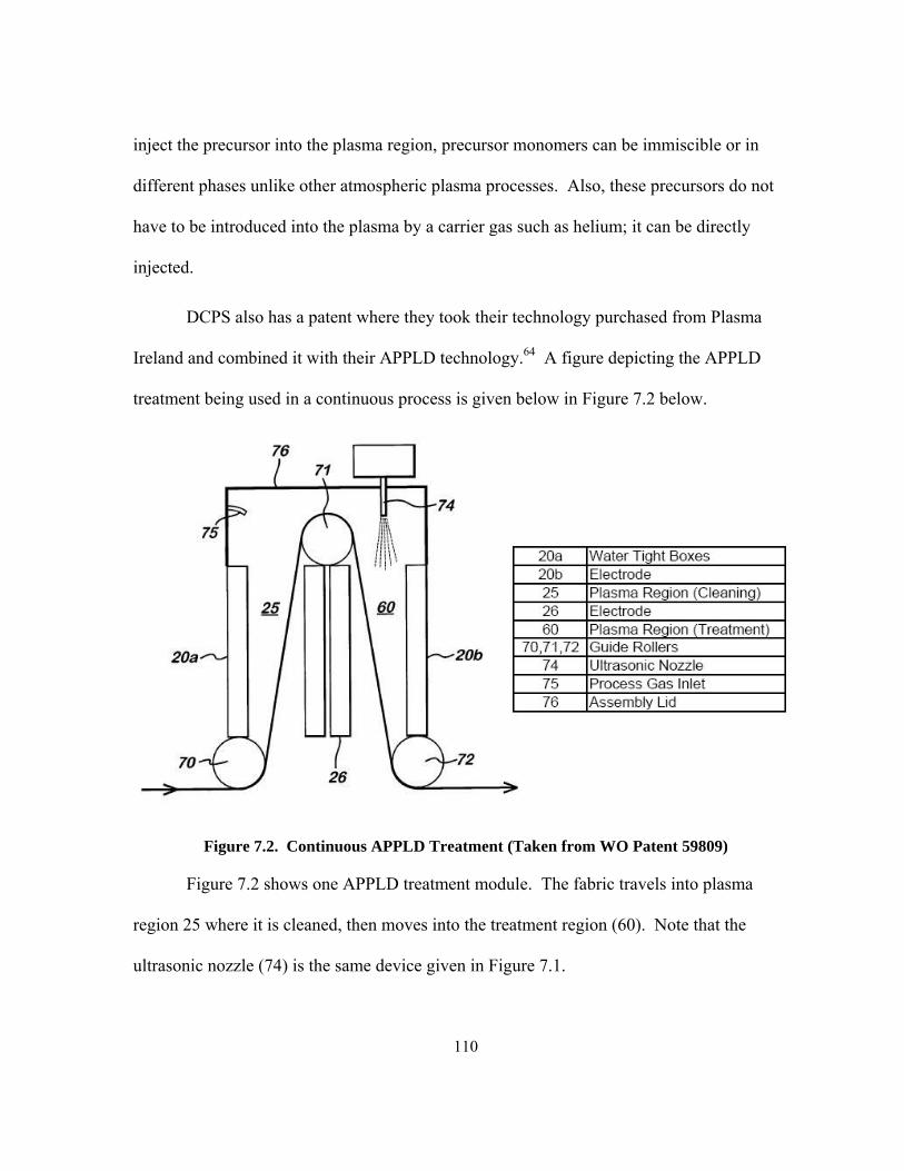
110
inject the precursor into the plasma region, precursor monomers can be immiscible or in
different phases unlike other atmospheric plasma processes. Also, these precursors do not
have to be introduced into the plasma by a carrier gas such as helium; it can be directly
injected.
DCPS also has a patent where they took their technology purchased from Plasma
Ireland and combined it with their APPLD technology.64 A figure depicting the APPLD
treatment being used in a continuous process is given below in Figure 7.2 below.
Figure 7.2. Continuous APPLD Treatment (Taken from WO Patent 59809)
Figure 7.2 shows one APPLD treatment module. The fabric travels into plasma
region 25 where it is cleaned, then moves into the treatment region (60). Note that the
ultrasonic nozzle (74) is the same device given in Figure 7.1.

111
The machine that was used in this research was the SE-1100 LabLine platform,
shown in Figure 7.374 below, that is a stand alone, reel-to-reel surface engineering system for
flexible web materials up to 12.5 inches wide. The web is handled by an unwind/rewind
system with a maximum reel mass of 100 kilograms and a maximum line speed of 20 meters
per minute. This machine is used to simulate the results which would be possible on their
full width SE-1000 AP4 machine.
Figure 7.3. DCPS SE-1100 LabLine Machine
The SE-1000 AP4 machine from DCPS, shown in Figure 7.475, is capable of treating
fabrics up to 2.5 meters (98 inches) wide. Individual modules can be purchased for multiple
treatments or multiple passes. It can be configured for either in-line production or as a stand
alone system with the addition of web handling equipment. The foot print of the SE-1000
AP4 machine is 2 meters wide by 3.8 meters long and is 3.3 meters high. DCPS has
provided an approximate cost of a 3 station SE-1000 AP4 machine that will allow three

112
passes as performed in this research to be between 2.5 and 4 million US dollars depending on
the need for web handling equipment, and the amount of integration into the current
production line. The SE-1000 AP4 requires one operator.
Figure 7.4. DCPS SE-1000 AP4 Machine

113
Appendix B: X-ray Photoelectron Spectroscopy (XPS)
All information in this appendix has been taken from the book Handbook of X-ray
Photoelectron Spectroscopy.76
XPS is a surface analysis technique that irradiates a sample with monoenergetic soft
x-rays and analyzes the energy of the electrons that are emitted from the surface. There are
three different types of x-rays that can be used. In this study Mg Kα (1486.7 eV) x-rays were
used exclusively. These photons interact with atoms only 1-10 microns into the surface
because they have limited penetrating power. The photons cause electrons on the surface to
be emitted by the photoelectric effect. These electrons have a kinetic energy which can be
measured. From this kinetic energy, the binding energy of the atomic orbital from which the
electron originated can be determined by subtracting out the energy of the photon and the
spectrometer work function.
The measured binding energies of electrons are the key to XPS. Binding energies can
be defined as the difference between the initial and final states after the photoelectron has left
the atom that was bombarded by the x-rays. Electron binding energies are unique to each
element in the periodic table. Because XPS can measure these binding energies, it can be
used to both identify and determine the concentration of elements on the surface.
In order to produce the binding energy spectra, electrons leaving the surface are
detected by an electron spectrometer according to their kinetic energy. The analyzer can
only accept electrons at a specific kinetic energy. A variable electrostatic field is placed

114
before the analyzer in order to determine the different energies of the electrons. The
electrons are detected as discrete events. The number of electrons detected in a given time is
given on the y-axis and the binding energy of the electron is displayed on the x-axis.
The electrons that leave the surface without energy loss produce peaks in the spectra.
There is usually multiple spikes due to one element. This is because roughly 10-14 seconds
after the photoelectric event, excited ions emit Auger electrons. Software packages are used
to analyze the XPS spectrum to determine what elements are present on the surface and in
what quantities.
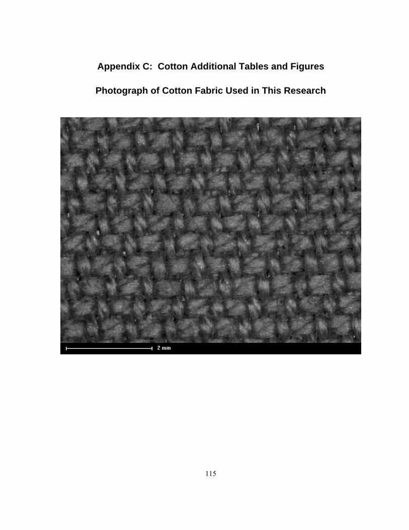
115
Appendix C: Cotton Additional Tables and Figures
Photograph of Cotton Fabric Used in This Research

116
Appendix C: XPS Binding Energy Scan of Cotton
Fl 1
s
Fl A
uger
Pea
ks
O 1
s
C 1
s
Fl 1
s
Fl A
uger
Pea
ks
O 1
s
C 1
s
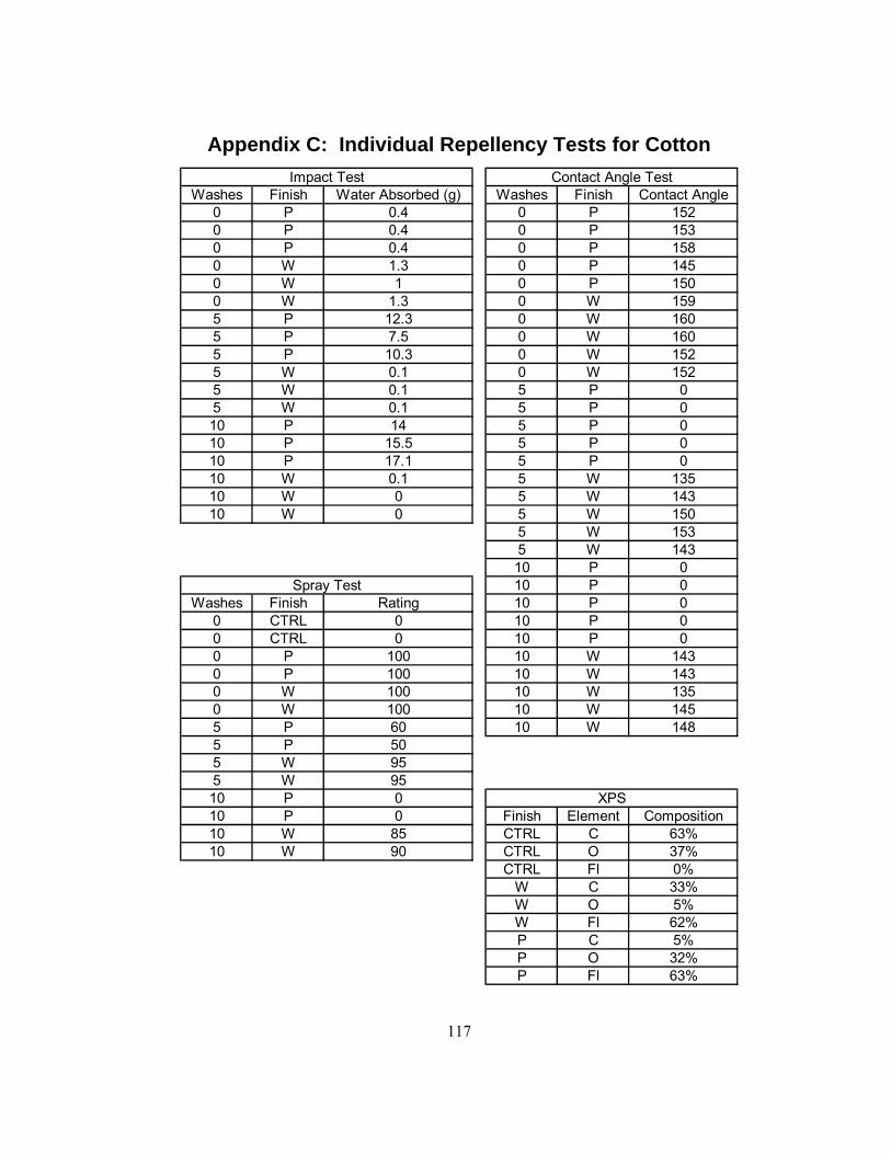
117
Appendix C: Individual Repellency Tests for Cotton
Washes Finish Water Absorbed (g) Washes Finish Contact Angle0 P 0.4 0 P 1520 P 0.4 0 P 1530 P 0.4 0 P 1580 W 1.3 0 P 1450 W 1 0 P 1500 W 1.3 0 W 1595 P 12.3 0 W 1605 P 7.5 0 W 1605 P 10.3 0 W 1525 W 0.1 0 W 1525 W 0.1 5 P 05 W 0.1 5 P 010 P 14 5 P 010 P 15.5 5 P 010 P 17.1 5 P 010 W 0.1 5 W 13510 W 0 5 W 14310 W 0 5 W 150
5 W 1535 W 14310 P 010 P 0
Washes Finish Rating 10 P 00 CTRL 0 10 P 00 CTRL 0 10 P 00 P 100 10 W 1430 P 100 10 W 1430 W 100 10 W 1350 W 100 10 W 1455 P 60 10 W 1485 P 505 W 955 W 9510 P 010 P 0 Finish Element Composition10 W 85 CTRL C 63%10 W 90 CTRL O 37%
CTRL Fl 0%W C 33%W O 5%W Fl 62%P C 5%P O 32%P Fl 63%
XPS
Impact Test Contact Angle Test
Spray Test

118
Appendix C: Contact Angle ANOVA between Finishes (Cotton) As Received
130
135
140
145
150
155
160
165C
onta
ct A
ngle
P W
Finish
RsquareAdj RsquareRoot Mean Square ErrorMean of ResponseObservations (or Sum Wgts)
0.2803950.1904444.477723
154.110
Summary of Fit
W-PAssuming equal variancesDifferenceStd Err DifUpper CL DifLower CL DifConfidence
5.0002.832
11.531-1.531
0.95
t RatioDFProb > |t|Prob > tProb < t
1.7655618
0.11550.05770.9423 -10 -5 0 5 10
t Test
FinishErrorC. Total
Source189
DF62.50000
160.40000222.90000
Sum of Squares62.500020.0500
Mean Square3.1172F Ratio
0.1155Prob > F
Analysis of Variance
PW
Level55
Number151.600156.600
Mean2.00252.0025
Std Error146.98151.98
Lower 95%156.22161.22
Upper 95%
Std Error uses a pooled estimate of error variance
Means for Oneway Anova
Oneway Anova
Oneway Analysis of Contact Angle By Finish Washes=0
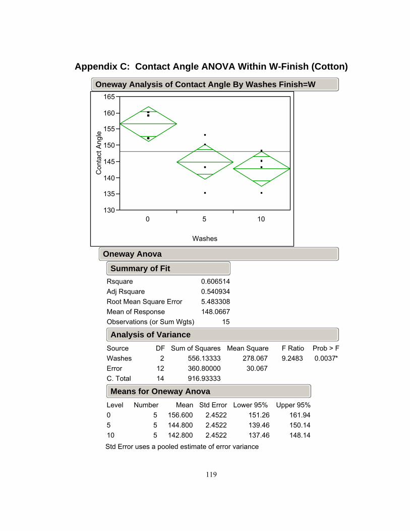
119
Appendix C: Contact Angle ANOVA Within W-Finish (Cotton)
130
135
140
145
150
155
160
165C
onta
ct A
ngle
0 5 10
Washes
RsquareAdj RsquareRoot Mean Square ErrorMean of ResponseObservations (or Sum Wgts)
0.6065140.5409345.483308148.0667
15
Summary of Fit
WashesErrorC. Total
Source2
1214
DF556.13333360.80000916.93333
Sum of Squares278.06730.067
Mean Square9.2483F Ratio
0.0037*Prob > F
Analysis of Variance
0510
Level555
Number156.600144.800142.800
Mean2.45222.45222.4522
Std Error151.26139.46137.46
Lower 95%161.94150.14148.14
Upper 95%
Std Error uses a pooled estimate of error variance
Means for Oneway Anova
Oneway Anova
Oneway Analysis of Contact Angle By Washes Finish=W

120
Appendix D: Polyester/Cotton Additional Tables and Figures
Photograph of Polyester/Cotton Fabric Used in This Research
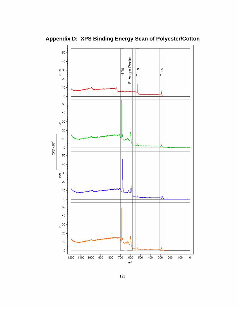
121
Appendix D: XPS Binding Energy Scan of Polyester/Cotton
Fl 1
s
Fl A
uger
Pea
ks
O 1
s
C 1
s
Fl 1
s
Fl A
uger
Pea
ks
O 1
s
C 1
s

122
Appendix D: Individual Repellency Tests for Polyester/Cotton
Washes Finish Rating Washes Finish Water Absorbed (g) Finish Element Composition0 CTRL 0 0 P 15.2 CTRL C 65%0 CTRL 0 0 P 14.9 CTRL O 35%0 CTRL 0 0 P 15.9 W C 31%0 P 95 0 W 5.3 W O 4%0 P 95 0 W 6.6 W F 65%0 P 100 0 W 4.9 WM C 33%0 W 100 0 WM 8.9 WM O 5%0 W 100 0 WM 9.3 WM F 60%0 W 100 5 P 11.8 WM N 2%0 WM 100 5 P 16.9 P C 32%0 WM 100 5 P 16.9 P O 4%0 WM 100 5 W 2.4 P F 64%5 P 80 5 W 4.35 P 80 5 W 4.15 P 80 5 WM 85 W 100 5 WM 75 W 100 5 WM 7.65 W 100 10 P 15.45 WM 100 10 P 16.15 WM 100 10 P 17.15 WM 100 10 W 3.710 P 70 10 W 3.810 P 70 10 W 2.910 P 70 10 WM 7.510 W 100 10 WM 4.710 W 100 10 WM 210 W 100 25 P 17.410 WM 95 25 P 16.910 WM 100 25 P 16.610 WM 100 25 W 1.825 P 50 25 W 1.625 P 50 25 W 0.825 P 60 25 WM 3.825 W 95 25 WM 4.125 W 100 25 WM 3.825 W 10025 WM 9025 WM 9025 WM 95
Spray Test Impact Test XPS Test

123
Appendix D: Individual Repellency Tests for Polyester/Cotton (cont.)
Contact Angle Test Washes Finish Contact Angle Washes Finish Contact Angle
0 P 155 10 P 138 0 P 156 10 P 140 0 P 148 10 P 143 0 P 145 10 P 140 0 P 148 10 P 147 0 W 153 10 W 148 0 W 151 10 W 156 0 W 145 10 W 153 0 W 148 10 W 157 0 W 152 10 W 150 0 WM 163 10 WM 158 0 WM 154 10 WM 148 0 WM 153 10 WM 158 0 WM 158 10 WM 148 0 WM 151 10 WM 157 5 P 152 25 P 135 5 P 145 25 P 132 5 P 147 25 P 135 5 P 147 25 P 140 5 P 140 25 P 147 5 W 156 25 W 148 5 W 154 25 W 150 5 W 155 25 W 154 5 W 158 25 W 152 5 W 152 25 W 149 5 WM 154 25 WM 155 5 WM 162 25 WM 150 5 WM 155 25 WM 149 5 WM 159 25 WM 149 5 WM 146 25 WM 159
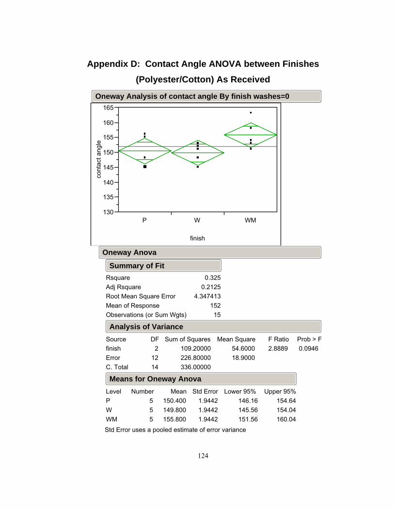
124
Appendix D: Contact Angle ANOVA between Finishes (Polyester/Cotton) As Received
130
135
140
145
150
155
160
165co
ntac
t ang
le
P W WM
finish
RsquareAdj RsquareRoot Mean Square ErrorMean of ResponseObservations (or Sum Wgts)
0.3250.2125
4.34741315215
Summary of Fit
finishErrorC. Total
Source2
1214
DF109.20000226.80000336.00000
Sum of Squares54.600018.9000
Mean Square2.8889F Ratio
0.0946Prob > F
Analysis of Variance
PWWM
Level555
Number150.400149.800155.800
Mean1.94421.94421.9442
Std Error146.16145.56151.56
Lower 95%154.64154.04160.04
Upper 95%
Std Error uses a pooled estimate of error variance
Means for Oneway Anova
Oneway Anova
Oneway Analysis of contact angle By finish washes=0

125
Appendix D: Contact Angle ANOVA between Finishes (Polyester/Cotton) at 5 Washes
130
135
140
145
150
155
160
165co
ntac
t ang
le
P W WM
finish
RsquareAdj RsquareRoot Mean Square ErrorMean of ResponseObservations (or Sum Wgts)
0.5222780.4426584.487018152.1333
15
Summary of Fit
finishErrorC. Total
Source2
1214
DF264.13333241.60000505.73333
Sum of Squares132.06720.133
Mean Square6.5596F Ratio
0.0119*Prob > F
Analysis of Variance
PWWM
Level555
Number146.200155.000155.200
Mean2.00672.00672.0067
Std Error141.83150.63150.83
Lower 95%150.57159.37159.57
Upper 95%
Std Error uses a pooled estimate of error variance
Means for Oneway Anova
Oneway Anova
Oneway Analysis of contact angle By finish washes=5

126
Appendix D: Contact Angle ANOVA between Finishes (Polyester/Cotton) at 10 Washes
130
135
140
145
150
155
160
165co
ntac
t ang
le
P W WM
finish
RsquareAdj RsquareRoot Mean Square ErrorMean of ResponseObservations (or Sum Wgts)
0.6751030.6209544.289522
149.415
Summary of Fit
finishErrorC. Total
Source2
1214
DF458.80000220.80000679.60000
Sum of Squares229.40018.400
Mean Square12.4674F Ratio
0.0012*Prob > F
Analysis of Variance
PWWM
Level555
Number141.600152.800153.800
Mean1.91831.91831.9183
Std Error137.42148.62149.62
Lower 95%145.78156.98157.98
Upper 95%
Std Error uses a pooled estimate of error variance
Means for Oneway Anova
Oneway Anova
Oneway Analysis of contact angle By finish washes=10

127
Appendix D: Contact Angle ANOVA between Finishes (Polyester/Cotton) at 25 Washes
130
135
140
145
150
155
160
165co
ntac
t ang
le
P W WM
finish
RsquareAdj RsquareRoot Mean Square ErrorMean of ResponseObservations (or Sum Wgts)
0.7243220.6783754.483302146.9333
15
Summary of Fit
finishErrorC. Total
Source2
1214
DF633.73333241.20000874.93333
Sum of Squares316.86720.100
Mean Square15.7645F Ratio
0.0004*Prob > F
Analysis of Variance
PWWM
Level555
Number137.800150.600152.400
Mean2.00502.00502.0050
Std Error133.43146.23148.03
Lower 95%142.17154.97156.77
Upper 95%
Std Error uses a pooled estimate of error variance
Means for Oneway Anova
Oneway Anova
Oneway Analysis of contact angle By finish washes=25

128
Appendix D: Contact Angle ANOVA within Finishes (Polyester/Cotton) W Finish
130
135
140
145
150
155
160
165co
ntac
t ang
le
0 5 10 25
washes
RsquareAdj RsquareRoot Mean Square ErrorMean of ResponseObservations (or Sum Wgts)
0.3619740.2423443.008322
152.0520
Summary of Fit
washesErrorC. Total
Source3
1619
DF82.15000
144.80000226.95000
Sum of Squares27.38339.0500
Mean Square3.0258F Ratio
0.0602Prob > F
Analysis of Variance
051025
Level5555
Number149.800155.000152.800150.600
Mean1.34541.34541.34541.3454
Std Error146.95152.15149.95147.75
Lower 95%152.65157.85155.65153.45
Upper 95%
Std Error uses a pooled estimate of error variance
Means for Oneway Anova
Oneway Anova
Oneway Analysis of contact angle By washes finish=W

129
Appendix D: Contact Angle ANOVA within Finishes (Polyester/Cotton) WM Finish
130
135
140
145
150
155
160
165co
ntac
t ang
le
0 5 10 25
washes
RsquareAdj RsquareRoot Mean Square ErrorMean of ResponseObservations (or Sum Wgts)
0.074537-0.098995.181699
154.320
Summary of Fit
washesErrorC. Total
Source3
1619
DF34.60000
429.60000464.20000
Sum of Squares11.533326.8500
Mean Square0.4295F Ratio
0.7346Prob > F
Analysis of Variance
051025
Level5555
Number155.800155.200153.800152.400
Mean2.31732.31732.31732.3173
Std Error150.89150.29148.89147.49
Lower 95%160.71160.11158.71157.31
Upper 95%
Std Error uses a pooled estimate of error variance
Means for Oneway Anova
Oneway Anova
Oneway Analysis of contact angle By washes finish=WM

130
Appendix D: Contact Angle ANOVA within Finishes (Polyester/Cotton) P Finish
130
135
140
145
150
155
160
165co
ntac
t ang
le
0 5 10 25
washes
RsquareAdj RsquareRoot Mean Square ErrorMean of ResponseObservations (or Sum Wgts)
0.5583130.4754964.716991
14420
Summary of Fit
washesErrorC. Total
Source3
1619
DF450.00000356.00000806.00000
Sum of Squares150.00022.250
Mean Square6.7416F Ratio
0.0038*Prob > F
Analysis of Variance
051025
Level5555
Number150.400146.200141.600137.800
Mean2.10952.10952.10952.1095
Std Error145.93141.73137.13133.33
Lower 95%154.87150.67146.07142.27
Upper 95%
Std Error uses a pooled estimate of error variance
Means for Oneway Anova
Oneway Anova
Oneway Analysis of contact angle By washes finish=P

131
Appendix E: Polyester Additional Tables and Figures
Photograph of Calendered Polyester Fabric Used in This Research

132
Appendix E: Photograph of Non-Calendered Polyester Used in This Research

133
Appendix E: XPS Binding Energy Scan of Polyester
Fl 1
s
Fl A
uger
Pea
ks
O 1
s
C 1
s
Fl 1
s
Fl A
uger
Pea
ks
O 1
s
C 1
s

134
Appendix E: Individual Repellency Tests for Polyester
Washes Finish Rating Washes Finish Water Absorbed (g) Finish Element Composition0 C-CTRL 0 0 C-P 0.1 C-CTRL C 82%0 C-CTRL 0 0 C-P 0 C-CTRL O 18%0 C-CTRL 0 0 C-P 0 NC-CTRL C 80%0 NC-CTRL 0 0 C-W 0 NC-CTRL O 20%0 NC-CTRL 0 0 C-W 0 C-W C 33%0 NC-CTRL 0 0 C-W 0 C-W O 4%0 C-P 100 0 NC-P 0.1 C-W Fl 63%0 C-P 100 0 NC-P 0.1 C-P C 32%0 C-P 100 0 NC-P 0.1 C-P O 5%0 C-W 100 5 C-P 0 C-P Fl 64%0 C-W 100 5 C-P 0.1 NC-P C 30%0 C-W 100 5 C-P 0 NC-P O 5%0 NC-P 100 5 C-W 0 NC-P Fl 65%0 NC-P 100 5 C-W 00 NC-P 100 5 C-W 0.15 C-P 100 5 NC-P 0.15 C-P 100 5 NC-P 0.15 C-P 100 5 NC-P 0.15 C-W 100 10 C-P 05 C-W 100 10 C-P 0.15 C-W 100 10 C-P 05 NC-P 100 10 C-W 05 NC-P 100 10 C-W 0.15 NC-P 100 10 C-W 010 C-P 100 10 NC-P 0.110 C-P 100 10 NC-P 0.110 C-P 100 10 NC-P 0.110 C-W 100 25 C-P 0.110 C-W 100 25 C-P 010 C-W 100 25 C-P 010 NC-P 100 25 C-W 010 NC-P 100 25 C-W 0.110 NC-P 100 25 C-W 025 C-P 100 25 NC-P 025 C-P 100 25 NC-P 0.125 C-P 100 25 NC-P 0.125 C-W 10025 C-W 10025 C-W 10025 NC-P 10025 NC-P 10025 NC-P 100
Spray Test Impact Test XPS Test

135
Appendix E: Individual Repellency Tests for Polyester (cont.)
Contact Angle Test Washes Finish Contact Angle Washes Finish Contact Angle
0 C-P 124 10 C-P 143 0 C-P 132 10 C-P 150 0 C-P 131 10 C-P 153 0 C-P 124 10 C-P 143 0 C-P 125 10 C-P 140 0 C-W 140 10 C-W 141 0 C-W 126 10 C-W 145 0 C-W 122 10 C-W 143 0 C-W 131 10 C-W 146 0 C-W 135 10 C-W 143 0 NC-P 152 10 NC-P 151 0 NC-P 158 10 NC-P 151 0 NC-P 162 10 NC-P 156 0 NC-P 158 10 NC-P 151 0 NC-P 147 10 NC-P 156 5 C-P 142 25 C-P 150 5 C-P 146 25 C-P 152 5 C-P 148 25 C-P 148 5 C-P 133 25 C-P 135 5 C-P 140 25 C-P 140 5 C-W 145 25 C-W 138 5 C-W 142 25 C-W 148 5 C-W 140 25 C-W 146 5 C-W 143 25 C-W 148 5 C-W 143 25 C-W 144 5 NC-P 147 25 NC-P 153 5 NC-P 148 25 NC-P 153 5 NC-P 153 25 NC-P 149 5 NC-P 149 25 NC-P 158 5 NC-P 158 25 NC-P 156

136
Appendix E: Individual Additional Test Results for Polyester
Washes Finish Water Pressure (cm) Washes Finish Permeability (cfm) Finish Warp Fill0 C-P 91.0 0 C-CTRL 0.44 C-W 0.6% 0.0%0 C-P 98.7 0 NC-CTRL 9.40 C-W 0.6% 0.0%0 C-P 97.0 0 C-P 0.36 C-W 0.6% 0.0%0 C-W 67.5 0 C-P 0.28 C-W 0.6% 0.0%0 C-W 67.0 0 C-P 0.35 C-W 0.6% 0.0%0 C-W 66.8 0 C-W 0.75 C-W 1.3% 0.3%0 NC-P 41.2 0 C-W 0.74 NC-P 3.8% 0.0%0 NC-P 40.8 0 C-W 0.74 NC-P 3.8% 0.0%0 NC-P 43.0 0 NC-P 7.74 NC-P 4.4% 0.0%5 C-P 80.8 0 NC-P 7.91 NC-P 3.8% 0.0%5 C-P 79.9 0 NC-P 8.03 NC-P 3.8% 0.3%5 C-P 78.5 5 C-P 0.45 NC-P 3.8% 0.0%5 C-W 80.9 5 C-P 0.41 C-P 1.9% 0.6%5 C-W 77.7 5 C-P 0.40 C-P 2.5% 0.6%5 C-W 79.9 5 C-W 0.74 C-P 2.5% 0.6%5 NC-P 41.9 5 C-W 0.74 C-P 2.2% 0.6%5 NC-P 40.8 5 C-W 0.74 C-P 1.9% 0.6%5 NC-P 41.5 5 NC-P 9.96 C-P 1.9% 0.6%10 C-P 77.0 5 NC-P 10.4010 C-P 74.2 5 NC-P 10.3010 C-P 76.3 10 C-P 0.8610 C-W 71.5 10 C-P 0.8610 C-W 69.1 10 C-P 0.8610 C-W 72.3 10 C-W 0.7910 NC-P 44.1 10 C-W 0.7710 NC-P 39.0 10 C-W 0.7610 NC-P 42.3 10 NC-P 9.7825 C-P 70.0 10 NC-P 10.1025 C-P 73.8 10 NC-P 9.5325 C-P 68.6 25 C-P 1.0125 C-W 72.3 25 C-P 1.0425 C-W 66.8 25 C-P 1.0025 C-W 63.0 25 C-W 0.7825 NC-P 41.7 25 C-W 0.7725 NC-P 42.2 25 C-W 0.7825 NC-P 44.2 25 NC-P 9.86
25 NC-P 10.1025 NC-P 10.00
Air PermeabilityHydrostatic Pressure Test 5 Wash Shrinkage Test

137
Appendix E: Individual Additional Test Results for Polyester (cont.)
Tensile Test Washes Finish Warp (lb) Fill (lb) Washes Finish Warp (lb) Fill (lb)
0 C-CTRL 183.2 103.8 5 NC-P 177.9 107.7 0 C-CTRL 180.2 105.6 5 NC-P 169.6 111.3 0 C-CTRL 181.1 99.1 5 NC-P 164.8 109.3 0 C-CTRL 187 106.6 5 NC-P 170.3 111.4 0 C-CTRL 189.1 104.7 5 NC-P 174.1 108 0 NC-CTRL 180.2 109.7 10 C-P 174.9 110 0 NC-CTRL 181.7 110.1 10 C-P 175.6 105.7 0 NC-CTRL 180.4 105.5 10 C-P 171.1 103.6 0 NC-CTRL 184.2 104.6 10 C-P 180.4 104.7 0 NC-CTRL 180 111.1 10 C-P 173.6 108.6 0 C-P 173.4 105 10 C-W 172 100 0 C-P 163.5 110.2 10 C-W 179.1 104.2 0 C-P 167.7 102 10 C-W 174.5 102.6 0 C-P 169.2 105.7 10 C-W 172.6 92 0 C-P 171.1 113.2 10 C-W 175.8 99.7 0 C-W 177.9 97.3 10 NC-P 177.5 110.9 0 C-W 176.8 95.1 10 NC-P 176.4 111.1 0 C-W 174.5 105 10 NC-P 173.4 110.6 0 C-W 177 102.4 10 NC-P 178.7 109.2 0 C-W 177.7 99.3 10 NC-P 168.4 111.3 0 NC-P 180.4 109.5 25 C-P 170.3 98.9 0 NC-P 185.3 109.2 25 C-P 176.6 103.3 0 NC-P 168.5 108.3 25 C-P 174.1 102.4 0 NC-P 186.3 108.3 25 C-P 172.4 98.9 0 NC-P 163.4 102.5 25 C-P 172.6 93.9 5 C-P 177.2 99.4 25 C-W 171.7 104.9 5 C-P 172 103.8 25 C-W 171.5 107.8 5 C-P 176.4 103.8 25 C-W 177.2 103.1 5 C-P 167.6 103.8 25 C-W 165.2 100.8 5 C-P 169.8 101.9 25 C-W 163.5 101.2 5 C-W 179.6 91.2 25 NC-P 176.6 109.2 5 C-W 173.9 87.6 25 NC-P 170.3 103.9 5 C-W 176 90 25 NC-P 169.8 108.3 5 C-W 176.8 93.8 25 NC-P 167.7 108.5 5 C-W 167.8 86.9 25 NC-P 167.7 107.8

138
Appendix E: Contact Angle ANOVA between Finishes (Polyester) As Received
120
130
140
150
160
170co
ntac
t ang
le
C-P C-W NC-P
finish
RsquareAdj RsquareRoot Mean Square ErrorMean of ResponseObservations (or Sum Wgts)
0.8533550.8289145.80804
137.815
Summary of Fit
finishErrorC. Total
Source2
1214
DF2355.6000404.8000
2760.4000
Sum of Squares1177.80
33.73
Mean Square34.9150F Ratio
<.0001*Prob > F
Analysis of Variance
C-PC-WNC-P
Level555
Number127.200130.800155.400
Mean2.59742.59742.5974
Std Error121.54125.14149.74
Lower 95%132.86136.46161.06
Upper 95%
Std Error uses a pooled estimate of error variance
Means for Oneway Anova
Oneway Anova
Oneway Analysis of contact angle By finish washes=0
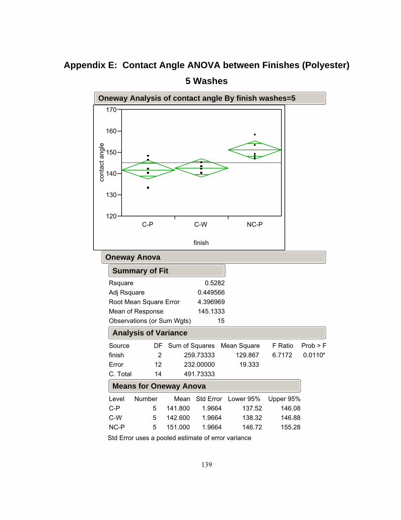
139
Appendix E: Contact Angle ANOVA between Finishes (Polyester) 5 Washes
120
130
140
150
160
170co
ntac
t ang
le
C-P C-W NC-P
finish
RsquareAdj RsquareRoot Mean Square ErrorMean of ResponseObservations (or Sum Wgts)
0.52820.4495664.396969145.1333
15
Summary of Fit
finishErrorC. Total
Source2
1214
DF259.73333232.00000491.73333
Sum of Squares129.86719.333
Mean Square6.7172F Ratio
0.0110*Prob > F
Analysis of Variance
C-PC-WNC-P
Level555
Number141.800142.600151.000
Mean1.96641.96641.9664
Std Error137.52138.32146.72
Lower 95%146.08146.88155.28
Upper 95%
Std Error uses a pooled estimate of error variance
Means for Oneway Anova
Oneway Anova
Oneway Analysis of contact angle By finish washes=5
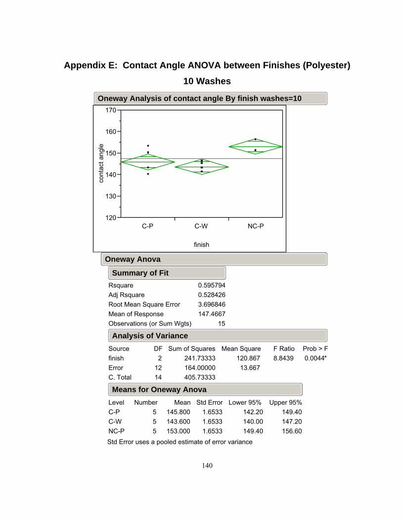
140
Appendix E: Contact Angle ANOVA between Finishes (Polyester) 10 Washes
120
130
140
150
160
170co
ntac
t ang
le
C-P C-W NC-P
finish
RsquareAdj RsquareRoot Mean Square ErrorMean of ResponseObservations (or Sum Wgts)
0.5957940.5284263.696846147.4667
15
Summary of Fit
finishErrorC. Total
Source2
1214
DF241.73333164.00000405.73333
Sum of Squares120.86713.667
Mean Square8.8439F Ratio
0.0044*Prob > F
Analysis of Variance
C-PC-WNC-P
Level555
Number145.800143.600153.000
Mean1.65331.65331.6533
Std Error142.20140.00149.40
Lower 95%149.40147.20156.60
Upper 95%
Std Error uses a pooled estimate of error variance
Means for Oneway Anova
Oneway Anova
Oneway Analysis of contact angle By finish washes=10
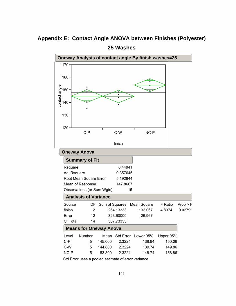
141
Appendix E: Contact Angle ANOVA between Finishes (Polyester) 25 Washes
120
130
140
150
160
170co
ntac
t ang
le
C-P C-W NC-P
finish
RsquareAdj RsquareRoot Mean Square ErrorMean of ResponseObservations (or Sum Wgts)
0.449410.3576455.192944147.8667
15
Summary of Fit
finishErrorC. Total
Source2
1214
DF264.13333323.60000587.73333
Sum of Squares132.06726.967
Mean Square4.8974F Ratio
0.0279*Prob > F
Analysis of Variance
C-PC-WNC-P
Level555
Number145.000144.800153.800
Mean2.32242.32242.3224
Std Error139.94139.74148.74
Lower 95%150.06149.86158.86
Upper 95%
Std Error uses a pooled estimate of error variance
Means for Oneway Anova
Oneway Anova
Oneway Analysis of contact angle By finish washes=25

142
Appendix E: Contact Angle ANOVA Within Finishes (Polyester) Calendered Conventional (C-W) Finish
120
130
140
150
160
170co
ntac
t ang
le
0 5 10 25
washes
RsquareAdj RsquareRoot Mean Square ErrorMean of ResponseObservations (or Sum Wgts)
0.6784390.6181474.330127
140.4520
Summary of Fit
washesErrorC. Total
Source3
1619
DF632.95000300.00000932.95000
Sum of Squares210.98318.750
Mean Square11.2524F Ratio
0.0003*Prob > F
Analysis of Variance
051025
Level5555
Number130.800142.600143.600144.800
Mean1.93651.93651.93651.9365
Std Error126.69138.49139.49140.69
Lower 95%134.91146.71147.71148.91
Upper 95%
Std Error uses a pooled estimate of error variance
Means for Oneway Anova
Oneway Anova
Oneway Analysis of contact angle By washes finish=C-W
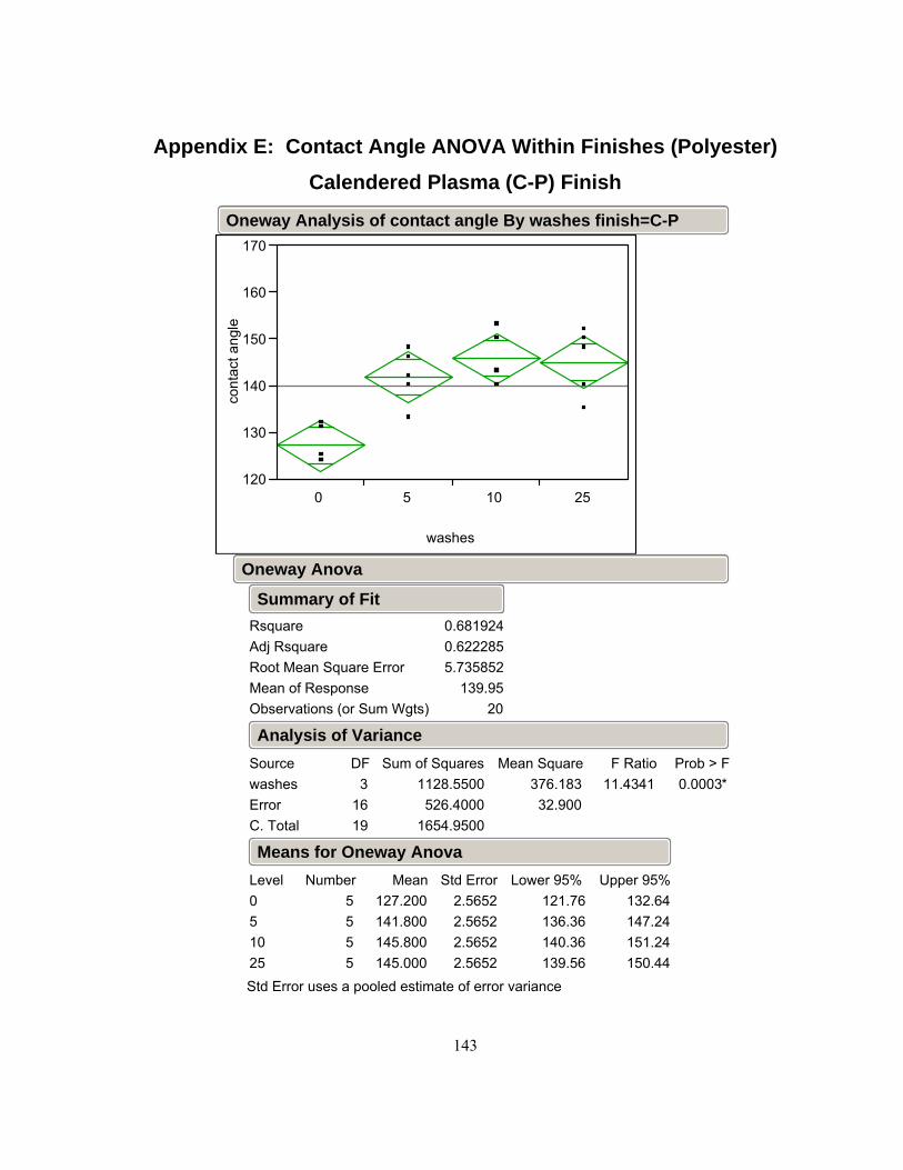
143
Appendix E: Contact Angle ANOVA Within Finishes (Polyester) Calendered Plasma (C-P) Finish
120
130
140
150
160
170co
ntac
t ang
le
0 5 10 25
washes
RsquareAdj RsquareRoot Mean Square ErrorMean of ResponseObservations (or Sum Wgts)
0.6819240.6222855.735852
139.9520
Summary of Fit
washesErrorC. Total
Source3
1619
DF1128.5500526.4000
1654.9500
Sum of Squares376.18332.900
Mean Square11.4341F Ratio
0.0003*Prob > F
Analysis of Variance
051025
Level5555
Number127.200141.800145.800145.000
Mean2.56522.56522.56522.5652
Std Error121.76136.36140.36139.56
Lower 95%132.64147.24151.24150.44
Upper 95%
Std Error uses a pooled estimate of error variance
Means for Oneway Anova
Oneway Anova
Oneway Analysis of contact angle By washes finish=C-P

144
Appendix E: Contact Angle ANOVA Within Finishes (Polyester) Non-Calendered Plasma (NC-P) Finish
120
130
140
150
160
170co
ntac
t ang
le
0 5 10 25
washes
RsquareAdj RsquareRoot Mean Square ErrorMean of ResponseObservations (or Sum Wgts)
0.14417-0.0163
4.315669153.3
20
Summary of Fit
washesErrorC. Total
Source3
1619
DF50.20000
298.00000348.20000
Sum of Squares16.733318.6250
Mean Square0.8984F Ratio
0.4635Prob > F
Analysis of Variance
051025
Level5555
Number155.400151.000153.000153.800
Mean1.93001.93001.93001.9300
Std Error151.31146.91148.91149.71
Lower 95%159.49155.09157.09157.89
Upper 95%
Std Error uses a pooled estimate of error variance
Means for Oneway Anova
Oneway Anova
Oneway Analysis of contact angle By washes finish=NC-P

145
Appendix E: Hydrostatic Pressure ANOVA Between Finishes (Polyester) As Received
60
70
80
90
100cm
C-P C-W
finish
Excluded Rows 3
RsquareAdj RsquareRoot Mean Square ErrorMean of ResponseObservations (or Sum Wgts)
0.9735790.9669742.87170181.33333
6
Summary of Fit
C-W-C-PAssuming equal variancesDifferenceStd Err DifUpper CL DifLower CL DifConfidence
-28.4672.345
-21.957-34.977
0.95
t RatioDFProb > |t|Prob > tProb < t
-12.14074
0.0003*0.99990.0001* -30 -20 -10 0 10 20 30
t Test
finishErrorC. Total
Source145
DF1215.5267
32.98671248.5133
Sum of Squares1215.53
8.25
Mean Square147.3961
F Ratio0.0003*
Prob > F
Analysis of Variance
C-PC-W
Level33
Number95.566767.1000
Mean1.65801.6580
Std Error90.96362.497
Lower 95%100.17
71.70
Upper 95%
Std Error uses a pooled estimate of error variance
Means for Oneway Anova
Oneway Anova
Oneway Analysis of cm By finish washes=0

146
Appendix E: Hydrostatic Pressure ANOVA Between Finishes (Polyester) 5 Washes
60
70
80
90
100cm
C-P C-W
finish
Excluded Rows 3
RsquareAdj RsquareRoot Mean Square ErrorMean of ResponseObservations (or Sum Wgts)
0.010047-0.237441.41833279.61667
6
Summary of Fit
C-W-C-PAssuming equal variancesDifferenceStd Err DifUpper CL DifLower CL DifConfidence
-0.23331.15812.9820
-3.44860.95
t RatioDFProb > |t|Prob > tProb < t
-0.201494
0.85020.57490.4251 -4 -3 -2 -1 0 1 2 3 4
t Test
finishErrorC. Total
Source145
DF0.08166678.04666678.1283333
Sum of Squares0.081672.01167
Mean Square0.0406F Ratio
0.8502Prob > F
Analysis of Variance
C-PC-W
Level33
Number79.733379.5000
Mean0.818870.81887
Std Error77.46077.226
Lower 95%82.00781.774
Upper 95%
Std Error uses a pooled estimate of error variance
Means for Oneway Anova
Oneway Anova
Oneway Analysis of cm By finish washes=5

147
Appendix E: Hydrostatic Pressure ANOVA Between Finishes (Polyester) 10 Washes
60
70
80
90
100cm
C-P C-W
finish
Excluded Rows 3
RsquareAdj RsquareRoot Mean Square ErrorMean of ResponseObservations (or Sum Wgts)
0.7839070.7298841.564715
73.46
Summary of Fit
C-W-C-PAssuming equal variancesDifferenceStd Err DifUpper CL DifLower CL DifConfidence
-4.86671.2776
-1.3195-8.4138
0.95
t RatioDFProb > |t|Prob > tProb < t
-3.809274
0.0190 *0.99050.0095 * -6 -5 -4 -3 -2 -1 0 1 2 3 4 5 6
t Test
finishErrorC. Total
Source145
DF35.526667
9.79333345.320000
Sum of Squares35.5267
2.4483
Mean Square14.5106
F Ratio0.0190 *
Prob > F
Analysis of Variance
C-PC-W
Level33
Number75.833370.9667
Mean0.903390.90339
Std Error73.32568.458
Lower 95%78.34273.475
Upper 95%
Std Error uses a pooled estimate of error variance
Means for Oneway Anova
Oneway Anova
Oneway Analysis of cm By finish washes=10

148
Appendix E: Hydrostatic Pressure ANOVA Between Finishes (Polyester) 25 Washes
60
70
80
90
100cm
C-P C-W
finish
Excluded Rows 3
RsquareAdj RsquareRoot Mean Square ErrorMean of ResponseObservations (or Sum Wgts)
0.2329960.0412453.81466569.08333
6
Summary of Fit
C-W-C-PAssuming equal variancesDifferenceStd Err DifUpper CL DifLower CL DifConfidence
-3.4333.1155.214
-12.0810.95
t RatioDFProb > |t|Prob > tProb < t
-1.102314
0.33220.83390.1661 -10 -5 0 5 10
t Test
finishErrorC. Total
Source145
DF17.68166758.20666775.888333
Sum of Squares17.681714.5517
Mean Square1.2151F Ratio
0.3322Prob > F
Analysis of Variance
C-PC-W
Level33
Number70.800067.3667
Mean2.20242.2024
Std Error64.68561.252
Lower 95%76.91573.482
Upper 95%
Std Error uses a pooled estimate of error variance
Means for Oneway Anova
Oneway Anova
Oneway Analysis of cm By finish washes=25

149
Appendix E: Hydrostatic Pressure ANOVA Within Finishes (Polyester) Calendered Conventional (C-W)
60
70
80
90
100cm
0 5 10 25
washes
RsquareAdj RsquareRoot Mean Square ErrorMean of ResponseObservations (or Sum Wgts)
0.8459030.7881172.61947871.23333
12
Summary of Fit
washesErrorC. Total
Source38
11
DF301.3333354.89333
356.22667
Sum of Squares100.444
6.862
Mean Square14.6385F Ratio
0.0013*Prob > F
Analysis of Variance
051025
Level3333
Number67.100079.500070.966767.3667
Mean1.51241.51241.51241.5124
Std Error63.61276.01267.47963.879
Lower 95%70.58882.98874.45470.854
Upper 95%
Std Error uses a pooled estimate of error variance
Means for Oneway Anova
Oneway Anova
Oneway Analysis of cm By washes finish=C-W

150
Appendix E: Hydrostatic Pressure ANOVA Within Finishes (Polyester) Calendered Plasma (C-P)
60
70
80
90
100cm
0 5 10 25
washes
RsquareAdj RsquareRoot Mean Square ErrorMean of ResponseObservations (or Sum Wgts)
0.9500790.9313592.60144280.48333
12
Summary of Fit
washesErrorC. Total
Source38
11
DF1030.3767
54.14001084.5167
Sum of Squares343.459
6.768
Mean Square50.7512F Ratio
<.0001*Prob > F
Analysis of Variance
051025
Level3333
Number95.566779.733375.833370.8000
Mean1.50191.50191.50191.5019
Std Error92.10376.27072.37067.337
Lower 95%99.03083.19779.29774.263
Upper 95%
Std Error uses a pooled estimate of error variance
Means for Oneway Anova
Oneway Anova
Oneway Analysis of cm By washes finish=C-P
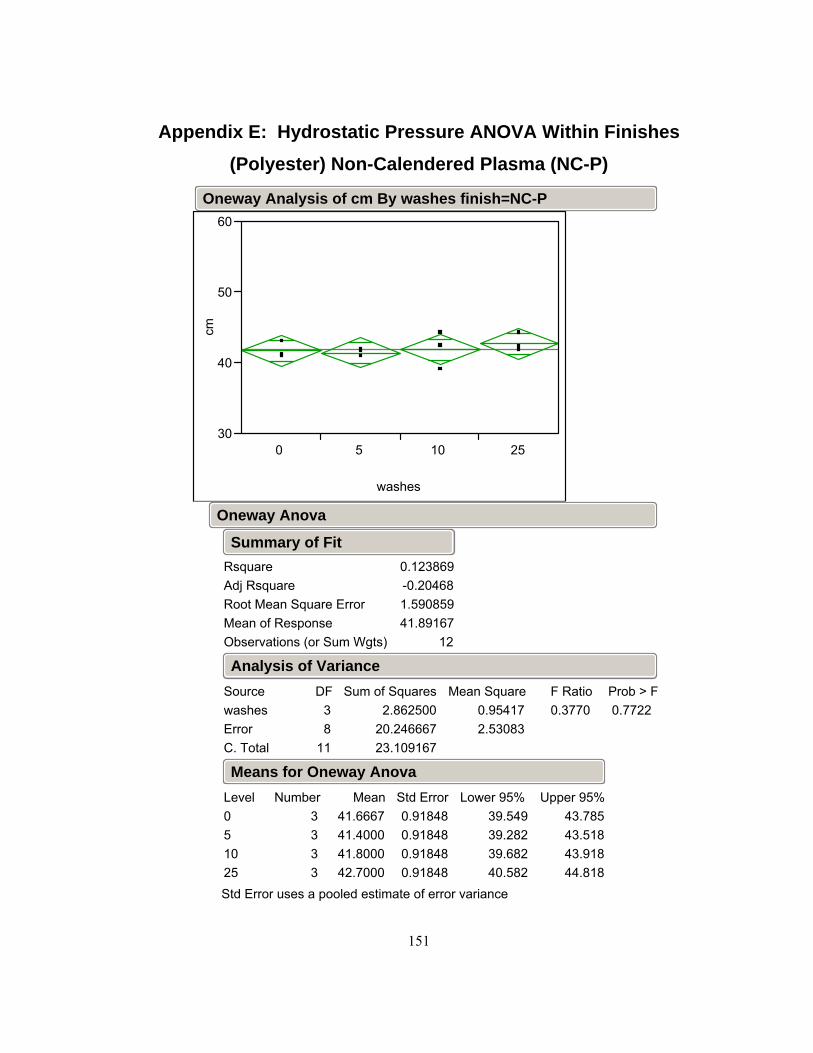
151
Appendix E: Hydrostatic Pressure ANOVA Within Finishes (Polyester) Non-Calendered Plasma (NC-P)
30
40
50
60cm
0 5 10 25
washes
RsquareAdj RsquareRoot Mean Square ErrorMean of ResponseObservations (or Sum Wgts)
0.123869-0.204681.59085941.89167
12
Summary of Fit
washesErrorC. Total
Source38
11
DF2.862500
20.24666723.109167
Sum of Squares0.954172.53083
Mean Square0.3770F Ratio
0.7722Prob > F
Analysis of Variance
051025
Level3333
Number41.666741.400041.800042.7000
Mean0.918480.918480.918480.91848
Std Error39.54939.28239.68240.582
Lower 95%43.78543.51843.91844.818
Upper 95%
Std Error uses a pooled estimate of error variance
Means for Oneway Anova
Oneway Anova
Oneway Analysis of cm By washes finish=NC-P

152
Appendix E: Air Permeability ANOVA Between Finishes (Polyester) As Received
0.2
0.4
0.6
0.8
1
1.2cf
m
C-P C-W
finish
Excluded Rows 3
RsquareAdj RsquareRoot Mean Square ErrorMean of ResponseObservations (or Sum Wgts)
0.9854670.981834
0.030540.535667
6
Summary of Fit
C-W-C-PAssuming equal variancesDifferenceStd Err DifUpper CL DifLower CL DifConfidence
0.4106670.0249350.4798990.341435
0.95
t RatioDFProb > |t|Prob > tProb < t
16.469184
<.0001*<.0001*1.0000 -0.5 -0.3 -0.1 .0 .1 .2 .3 .4 .5
t Test
finishErrorC. Total
Source145
DF0.252970670.003730670.25670133
Sum of Squares0.2529710.000933
Mean Square271.2337
F Ratio<.0001*
Prob > F
Analysis of Variance
C-PC-W
Level33
Number0.3303330.741000
Mean0.017630.01763
Std Error0.281380.69205
Lower 95%0.379290.78995
Upper 95%
Std Error uses a pooled estimate of error variance
Means for Oneway Anova
Oneway Anova
Oneway Analysis of cfm By finish washes=0

153
Appendix E: Air Permeability ANOVA Between Finishes (Polyester) 5 Washes
0.2
0.4
0.6
0.8
1
1.2cf
m
C-P C-W
finish
Excluded Rows 3
RsquareAdj RsquareRoot Mean Square ErrorMean of ResponseObservations (or Sum Wgts)
0.9908570.9885710.0187260.579167
6
Summary of Fit
C-W-C-PAssuming equal variancesDifferenceStd Err DifUpper CL DifLower CL DifConfidence
0.3183330.0152900.3607850.275882
0.95
t RatioDFProb > |t|Prob > tProb < t
20.819994
<.0001*<.0001*1.0000 -0.4 -0.3 -0.2 -0.1 .0 .1 .2 .3 .4
t Test
finishErrorC. Total
Source145
DF0.152004170.001402670.15340683
Sum of Squares0.1520040.000351
Mean Square433.4720
F Ratio<.0001*
Prob > F
Analysis of Variance
C-PC-W
Level33
Number0.4200000.738333
Mean0.010810.01081
Std Error0.389980.70832
Lower 95%0.450020.76835
Upper 95%
Std Error uses a pooled estimate of error variance
Means for Oneway Anova
Oneway Anova
Oneway Analysis of cfm By finish washes=5
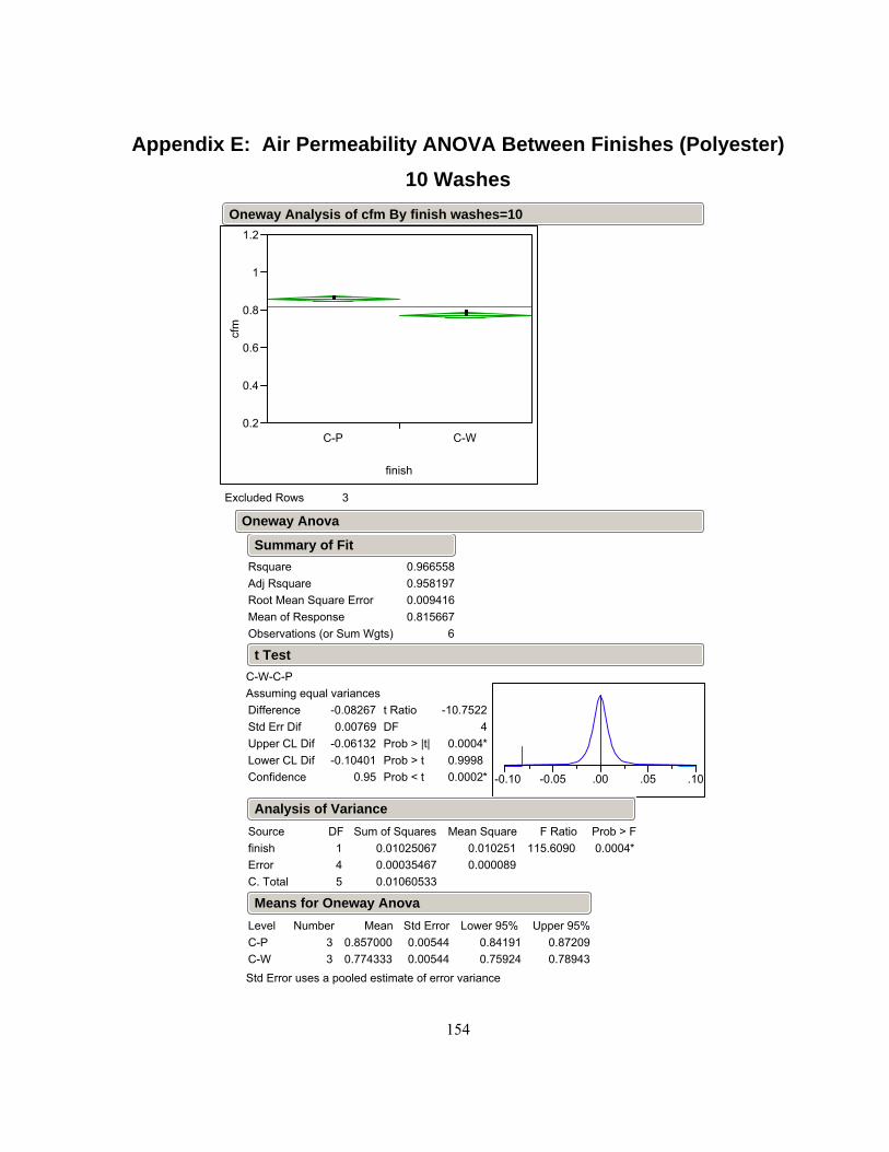
154
Appendix E: Air Permeability ANOVA Between Finishes (Polyester) 10 Washes
0.2
0.4
0.6
0.8
1
1.2cf
m
C-P C-W
finish
Excluded Rows 3
RsquareAdj RsquareRoot Mean Square ErrorMean of ResponseObservations (or Sum Wgts)
0.9665580.9581970.0094160.815667
6
Summary of Fit
C-W-C-PAssuming equal variancesDifferenceStd Err DifUpper CL DifLower CL DifConfidence
-0.082670.00769
-0.06132-0.10401
0.95
t RatioDFProb > |t|Prob > tProb < t
-10.75224
0.0004*0.99980.0002* -0.10 -0.05 .00 .05 .10
t Test
finishErrorC. Total
Source145
DF0.010250670.000354670.01060533
Sum of Squares0.0102510.000089
Mean Square115.6090
F Ratio0.0004*
Prob > F
Analysis of Variance
C-PC-W
Level33
Number0.8570000.774333
Mean0.005440.00544
Std Error0.841910.75924
Lower 95%0.872090.78943
Upper 95%
Std Error uses a pooled estimate of error variance
Means for Oneway Anova
Oneway Anova
Oneway Analysis of cfm By finish washes=10

155
Appendix E: Air Permeability ANOVA Between Finishes (Polyester) 25 Washes
0.2
0.4
0.6
0.8
1
1.2cf
m
C-P C-W
finish
Excluded Rows 3
RsquareAdj RsquareRoot Mean Square ErrorMean of ResponseObservations (or Sum Wgts)
0.9887880.9859850.0154540.898167
6
Summary of Fit
C-W-C-PAssuming equal variancesDifferenceStd Err DifUpper CL DifLower CL DifConfidence
-0.237000.01262
-0.20197-0.27203
0.95
t RatioDFProb > |t|Prob > tProb < t
-18.78224
<.0001*1.0000<.0001* -0.2 -0.1 .0 .1 .2
t Test
finishErrorC. Total
Source145
DF0.084253500.000955330.08520883
Sum of Squares0.0842540.000239
Mean Square352.7711
F Ratio<.0001*Prob > F
Analysis of Variance
C-PC-W
Level33
Number1.016670.77967
Mean0.008920.00892
Std Error0.991890.75489
Lower 95%1.04140.8044
Upper 95%
Std Error uses a pooled estimate of error variance
Means for Oneway Anova
Oneway Anova
Oneway Analysis of cfm By finish washes=25

156
Appendix E: Air Permeability ANOVA Within Finishes (Polyester) Calendered Conventional (C-W)
0.25
0.5
0.75
1
1.25cf
m
0 5 10 25
washes
Excluded Rows 30
RsquareAdj RsquareRoot Mean Square ErrorMean of ResponseObservations (or Sum Wgts)
0.8902590.8491070.0080780.758333
12
Summary of Fit
washesErrorC. Total
Source38
11
DF0.004234670.000522000.00475667
Sum of Squares0.0014120.000065
Mean Square21.6330F Ratio
0.0003*Prob > F
Analysis of Variance
051025
Level3333
Number0.7410000.7383330.7743330.779667
Mean0.004660.004660.004660.00466
Std Error0.730250.727580.763580.76891
Lower 95%0.751750.749090.785090.79042
Upper 95%
Std Error uses a pooled estimate of error variance
Means for Oneway Anova
Oneway Anova
Oneway Analysis of cfm By washes

157
Appendix E: Air Permeability ANOVA Within Finishes (Polyester) Calendered Plasma (C-P)
0.25
0.5
0.75
1
1.25cf
m
0 5 10 25
washes
Excluded Rows 30
RsquareAdj RsquareRoot Mean Square ErrorMean of ResponseObservations (or Sum Wgts)
0.9940940.99188
0.0272060.656
12
Summary of Fit
washesErrorC. Total
Source38
11
DF0.99670870.00592131.0026300
Sum of Squares0.3322360.000740
Mean Square448.8668
F Ratio<.0001*Prob > F
Analysis of Variance
051025
Level3333
Number0.330330.420000.857001.01667
Mean0.015710.015710.015710.01571
Std Error0.294110.383780.820780.98045
Lower 95%0.36660.45620.89321.0529
Upper 95%
Std Error uses a pooled estimate of error variance
Means for Oneway Anova
Oneway Anova
Oneway Analysis of cfm By washes
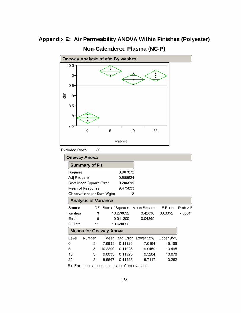
158
Appendix E: Air Permeability ANOVA Within Finishes (Polyester) Non-Calendered Plasma (NC-P)
7.5
8
8.5
9
9.5
10
10.5cf
m
0 5 10 25
washes
Excluded Rows 30
RsquareAdj RsquareRoot Mean Square ErrorMean of ResponseObservations (or Sum Wgts)
0.9678720.9558240.2065199.475833
12
Summary of Fit
washesErrorC. Total
Source38
11
DF10.2788920.341200
10.620092
Sum of Squares3.426300.04265
Mean Square80.3352F Ratio
<.0001*Prob > F
Analysis of Variance
051025
Level3333
Number7.8933
10.22009.80339.9867
Mean0.119230.119230.119230.11923
Std Error7.61849.94509.52849.7117
Lower 95%8.168
10.49510.07810.262
Upper 95%
Std Error uses a pooled estimate of error variance
Means for Oneway Anova
Oneway Anova
Oneway Analysis of cfm By washes

159
Appendix E: Warp Tensile ANOVA Between Finishes (Polyester) As Received
160
165
170
175
180W
arp
C-P C-W
Finish
Excluded Rows 15
RsquareAdj RsquareRoot Mean Square ErrorMean of ResponseObservations (or Sum Wgts)
0.7067980.6701472.80838172.88
10
Summary of Fit
C-W-C-PAssuming equal variancesDifferenceStd Err DifUpper CL DifLower CL DifConfidence
7.80001.7762
11.89593.7041
0.95
t RatioDFProb > |t|Prob > tProb < t
4.3914588
0.0023*0.0012*0.9988 -10 -5 0 5 10
t Test
FinishErrorC. Total
Source189
DF152.1000063.09600
215.19600
Sum of Squares152.100
7.887
Mean Square19.2849F Ratio
0.0023*Prob > F
Analysis of Variance
C-PC-W
Level55
Number168.980176.780
Mean1.25591.2559
Std Error166.08173.88
Lower 95%171.88179.68
Upper 95%
Std Error uses a pooled estimate of error variance
Means for Oneway Anova
Oneway Anova
Oneway Analysis of Warp By Finish Washes=0
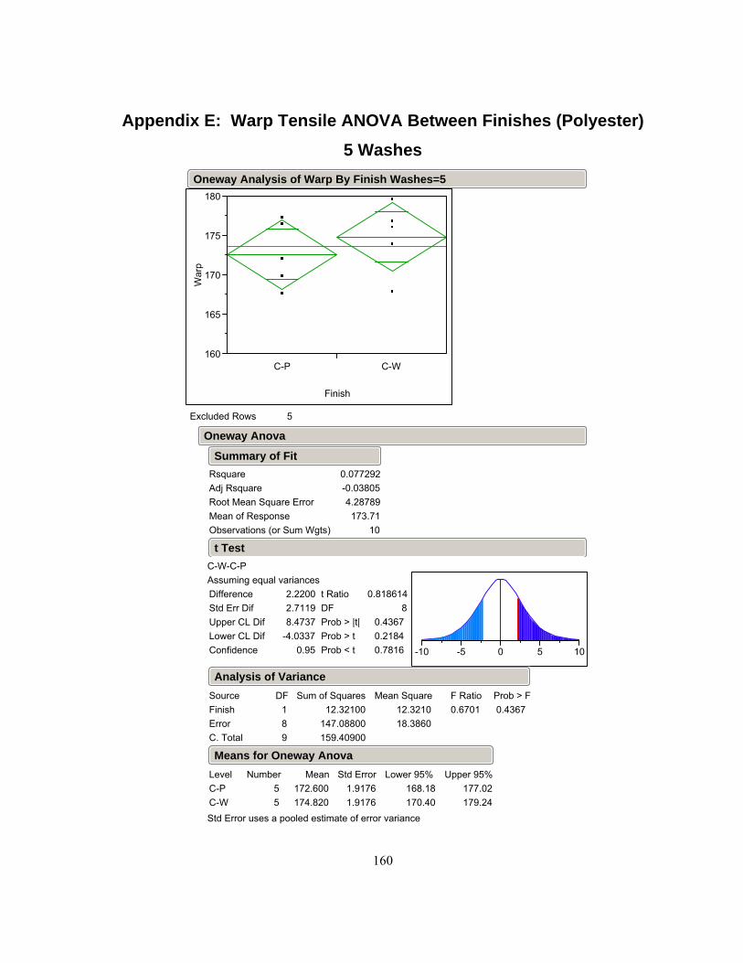
160
Appendix E: Warp Tensile ANOVA Between Finishes (Polyester) 5 Washes
160
165
170
175
180W
arp
C-P C-W
Finish
Excluded Rows 5
RsquareAdj RsquareRoot Mean Square ErrorMean of ResponseObservations (or Sum Wgts)
0.077292-0.038054.28789173.71
10
Summary of Fit
C-W-C-PAssuming equal variancesDifferenceStd Err DifUpper CL DifLower CL DifConfidence
2.22002.71198.4737
-4.03370.95
t RatioDFProb > |t|Prob > tProb < t
0.8186148
0.43670.21840.7816 -10 -5 0 5 10
t Test
FinishErrorC. Total
Source189
DF12.32100
147.08800159.40900
Sum of Squares12.321018.3860
Mean Square0.6701F Ratio
0.4367Prob > F
Analysis of Variance
C-PC-W
Level55
Number172.600174.820
Mean1.91761.9176
Std Error168.18170.40
Lower 95%177.02179.24
Upper 95%
Std Error uses a pooled estimate of error variance
Means for Oneway Anova
Oneway Anova
Oneway Analysis of Warp By Finish Washes=5

161
Appendix E: Warp Tensile ANOVA Between Finishes (Polyester) 10 Washes
160
165
170
175
180W
arp
C-P C-W
Finish
Excluded Rows 5
RsquareAdj RsquareRoot Mean Square ErrorMean of ResponseObservations (or Sum Wgts)
0.003235-0.121363.140223
174.9610
Summary of Fit
C-W-C-PAssuming equal variancesDifferenceStd Err DifUpper CL DifLower CL DifConfidence
-0.32001.98614.2598
-4.89980.95
t RatioDFProb > |t|Prob > tProb < t
-0.161128
0.87600.56200.4380 -6 -5 -4 -3 -2 -1 0 1 2 3 4 5 6
t Test
FinishErrorC. Total
Source189
DF0.256000
78.88800079.144000
Sum of Squares0.256009.86100
Mean Square0.0260F Ratio
0.8760Prob > F
Analysis of Variance
C-PC-W
Level55
Number175.120174.800
Mean1.40441.4044
Std Error171.88171.56
Lower 95%178.36178.04
Upper 95%
Std Error uses a pooled estimate of error variance
Means for Oneway Anova
Oneway Anova
Oneway Analysis of Warp By Finish Washes=10

162
Appendix E: Warp Tensile ANOVA Between Finishes (Polyester) 25 Washes
160
165
170
175
180W
arp
C-P C-W
Finish
Excluded Rows 5
RsquareAdj RsquareRoot Mean Square ErrorMean of ResponseObservations (or Sum Wgts)
0.165620.0613224.24099171.51
10
Summary of Fit
C-W-C-PAssuming equal variancesDifferenceStd Err DifUpper CL DifLower CL DifConfidence
-3.38002.68222.8053
-9.56530.95
t RatioDFProb > |t|Prob > tProb < t
-1.260148
0.24310.87840.1216 -10 -5 0 5 10
t Test
FinishErrorC. Total
Source189
DF28.56100
143.88800172.44900
Sum of Squares28.561017.9860
Mean Square1.5880F Ratio
0.2431Prob > F
Analysis of Variance
C-PC-W
Level55
Number173.200169.820
Mean1.89661.8966
Std Error168.83165.45
Lower 95%177.57174.19
Upper 95%
Std Error uses a pooled estimate of error variance
Means for Oneway Anova
Oneway Anova
Oneway Analysis of Warp By Finish Washes=25
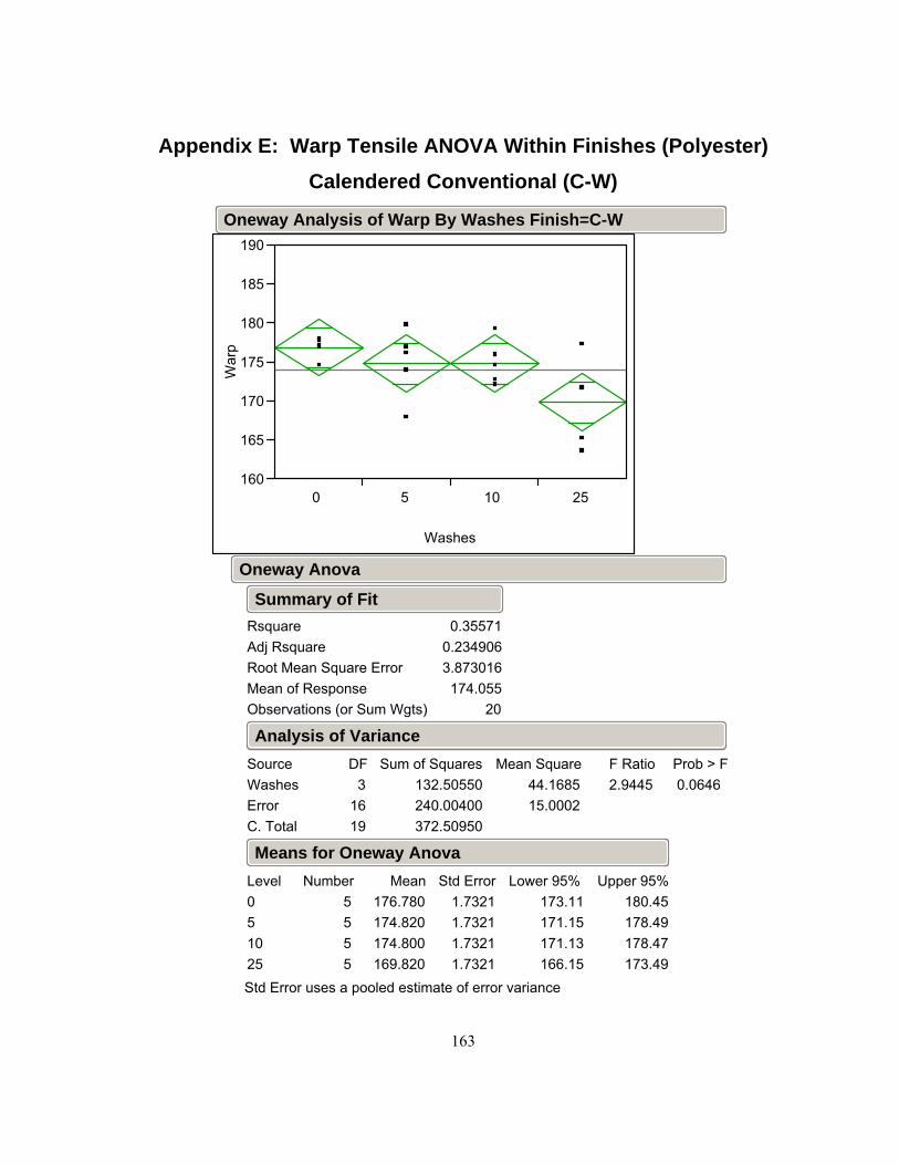
163
Appendix E: Warp Tensile ANOVA Within Finishes (Polyester) Calendered Conventional (C-W)
160
165
170
175
180
185
190W
arp
0 5 10 25
Washes
RsquareAdj RsquareRoot Mean Square ErrorMean of ResponseObservations (or Sum Wgts)
0.355710.2349063.873016174.055
20
Summary of Fit
WashesErrorC. Total
Source3
1619
DF132.50550240.00400372.50950
Sum of Squares44.168515.0002
Mean Square2.9445F Ratio
0.0646Prob > F
Analysis of Variance
051025
Level5555
Number176.780174.820174.800169.820
Mean1.73211.73211.73211.7321
Std Error173.11171.15171.13166.15
Lower 95%180.45178.49178.47173.49
Upper 95%
Std Error uses a pooled estimate of error variance
Means for Oneway Anova
Oneway Anova
Oneway Analysis of Warp By Washes Finish=C-W

164
Appendix E: Warp Tensile ANOVA Within Finishes (Polyester) Calendered Plasma (C-P)
160
165
170
175
180
185
190W
arp
0 5 10 25
Washes
RsquareAdj RsquareRoot Mean Square ErrorMean of ResponseObservations (or Sum Wgts)
0.3385520.21453
3.472715172.475
20
Summary of Fit
WashesErrorC. Total
Source3
1619
DF98.76150
192.95600291.71750
Sum of Squares32.920512.0598
Mean Square2.7298F Ratio
0.0783Prob > F
Analysis of Variance
051025
Level5555
Number168.980172.600175.120173.200
Mean1.55301.55301.55301.5530
Std Error165.69169.31171.83169.91
Lower 95%172.27175.89178.41176.49
Upper 95%
Std Error uses a pooled estimate of error variance
Means for Oneway Anova
Oneway Anova
Oneway Analysis of Warp By Washes Finish=C-P

165
Appendix E: Warp Tensile ANOVA Within Finishes (Polyester) Non-Calendered Plasma (NC-P)
160
165
170
175
180
185
190W
arp
0 5 10 25
Washes
RsquareAdj RsquareRoot Mean Square ErrorMean of ResponseObservations (or Sum Wgts)
0.1721390.0169156.338257173.355
20
Summary of Fit
WashesErrorC. Total
Source3
1619
DF133.65350642.77600776.42950
Sum of Squares44.551240.1735
Mean Square1.1090F Ratio
0.3745Prob > F
Analysis of Variance
051025
Level5555
Number176.780171.340174.880170.420
Mean2.83462.83462.83462.8346
Std Error170.77165.33168.87164.41
Lower 95%182.79177.35180.89176.43
Upper 95%
Std Error uses a pooled estimate of error variance
Means for Oneway Anova
Oneway Anova
Oneway Analysis of Warp By Washes Finish=NC-P

166
Appendix E: Fill Tensile ANOVA Between Finishes (Polyester) As Received
85
90
95
100
105
110
115Fi
ll
C-P C-W
Finish
Excluded Rows 15
RsquareAdj RsquareRoot Mean Square ErrorMean of ResponseObservations (or Sum Wgts)
0.491710.4281744.205889
103.5210
Summary of Fit
C-W-C-PAssuming equal variancesDifferenceStd Err DifUpper CL DifLower CL DifConfidence
-7.4002.660
-1.266-13.534
0.95
t RatioDFProb > |t|Prob > tProb < t
-2.781928
0.0239*0.98810.0119* -10 -5 0 5 10
t Test
FinishErrorC. Total
Source189
DF136.90000141.51600278.41600
Sum of Squares136.90017.689
Mean Square7.7391F Ratio
0.0239*Prob > F
Analysis of Variance
C-PC-W
Level55
Number107.22099.820
Mean1.88091.8809
Std Error102.8895.48
Lower 95%111.56104.16
Upper 95%
Std Error uses a pooled estimate of error variance
Means for Oneway Anova
Oneway Anova
Oneway Analysis of Fill By Finish Washes=0

167
Appendix E: Fill Tensile ANOVA Between Finishes (Polyester) 5 Washes
85
90
95
100
105
110
115Fi
ll
C-P C-W
Finish
Excluded Rows 5
RsquareAdj RsquareRoot Mean Square ErrorMean of ResponseObservations (or Sum Wgts)
0.8962610.8832932.403955
96.2210
Summary of Fit
C-W-C-PAssuming equal variancesDifferenceStd Err DifUpper CL DifLower CL DifConfidence
-12.6401.520
-9.134-16.146
0.95
t RatioDFProb > |t|Prob > tProb < t
-8.313638
<.0001*1.0000<.0001* -15 -10 -5 0 5 10 15
t Test
FinishErrorC. Total
Source189
DF399.4240046.23200
445.65600
Sum of Squares399.424
5.779
Mean Square69.1165F Ratio
<.0001*Prob > F
Analysis of Variance
C-PC-W
Level55
Number102.54089.900
Mean1.07511.0751
Std Error100.0687.42
Lower 95%105.0292.38
Upper 95%
Std Error uses a pooled estimate of error variance
Means for Oneway Anova
Oneway Anova
Oneway Analysis of Fill By Finish Washes=5

168
Appendix E: Fill Tensile ANOVA Between Finishes (Polyester) 10 Washes
85
90
95
100
105
110
115Fi
ll
C-P C-W
Finish
Excluded Rows 5
RsquareAdj RsquareRoot Mean Square ErrorMean of ResponseObservations (or Sum Wgts)
0.4984850.4357953.824069
103.1110
Summary of Fit
C-W-C-PAssuming equal variancesDifferenceStd Err DifUpper CL DifLower CL DifConfidence
-6.8202.419
-1.243-12.397
0.95
t RatioDFProb > |t|Prob > tProb < t
-2.819878
0.0225*0.98880.0112* -8 -6 -4 -2 0 2 4 6 8
t Test
FinishErrorC. Total
Source189
DF116.28100116.98800233.26900
Sum of Squares116.28114.623
Mean Square7.9517F Ratio
0.0225*Prob > F
Analysis of Variance
C-PC-W
Level55
Number106.52099.700
Mean1.71021.7102
Std Error102.5895.76
Lower 95%110.46103.64
Upper 95%
Std Error uses a pooled estimate of error variance
Means for Oneway Anova
Oneway Anova
Oneway Analysis of Fill By Finish Washes=10

169
Appendix E: Fill Tensile ANOVA Between Finishes (Polyester) 25 Washes
85
90
95
100
105
110
115Fi
ll
C-P C-W
Finish
Excluded Rows 5
RsquareAdj RsquareRoot Mean Square ErrorMean of ResponseObservations (or Sum Wgts)
0.3208240.2359273.318509
101.5210
Summary of Fit
C-W-C-PAssuming equal variancesDifferenceStd Err DifUpper CL DifLower CL DifConfidence
4.08002.09888.9199
-0.75990.95
t RatioDFProb > |t|Prob > tProb < t
1.9439598
0.08780.0439*0.9561 -8 -6 -4 -2 0 2 4 6 8
t Test
FinishErrorC. Total
Source189
DF41.6160088.10000
129.71600
Sum of Squares41.616011.0125
Mean Square3.7790F Ratio
0.0878Prob > F
Analysis of Variance
C-PC-W
Level55
Number99.480
103.560
Mean1.48411.4841
Std Error96.06
100.14
Lower 95%102.90106.98
Upper 95%
Std Error uses a pooled estimate of error variance
Means for Oneway Anova
Oneway Anova
Oneway Analysis of Fill By Finish Washes=25

170
Appendix E: Fill Tensile ANOVA Within Finishes (Polyester) Calendered Conventional (C-W)
85
90
95
100
105
110
115Fi
ll
0 5 10 25
Washes
RsquareAdj RsquareRoot Mean Square ErrorMean of ResponseObservations (or Sum Wgts)
0.7046320.6492513.664014
98.24520
Summary of Fit
WashesErrorC. Total
Source3
1619
DF512.42950214.80000727.22950
Sum of Squares170.81013.425
Mean Square12.7233F Ratio
0.0002*Prob > F
Analysis of Variance
051025
Level5555
Number99.82089.90099.700
103.560
Mean1.63861.63861.63861.6386
Std Error96.3586.4396.23
100.09
Lower 95%103.2993.37
103.17107.03
Upper 95%
Std Error uses a pooled estimate of error variance
Means for Oneway Anova
Oneway Anova
Oneway Analysis of Fill By Washes Finish=C-W

171
Appendix E: Fill Tensile ANOVA Within Finishes (Polyester) Calendered Plasma (C-P)
85
90
95
100
105
110
115Fi
ll
0 5 10 25
Washes
RsquareAdj RsquareRoot Mean Square ErrorMean of ResponseObservations (or Sum Wgts)
0.5244360.4352683.335753
103.9420
Summary of Fit
WashesErrorC. Total
Source3
1619
DF196.33200178.03600374.36800
Sum of Squares65.444011.1272
Mean Square5.8814F Ratio
0.0066*Prob > F
Analysis of Variance
051025
Level5555
Number107.220102.540106.52099.480
Mean1.49181.49181.49181.4918
Std Error104.0699.38
103.3696.32
Lower 95%110.38105.70109.68102.64
Upper 95%
Std Error uses a pooled estimate of error variance
Means for Oneway Anova
Oneway Anova
Oneway Analysis of Fill By Washes Finish=C-P

172
Appendix E: Fill Tensile ANOVA Within Finishes (Polyester) Non-Calendered Plasma (NC-P)
85
90
95
100
105
110
115Fi
ll
0 5 10 25
Washes
RsquareAdj RsquareRoot Mean Square ErrorMean of ResponseObservations (or Sum Wgts)
0.3464250.2238792.029224108.815
20
Summary of Fit
WashesErrorC. Total
Source3
1619
DF34.9215065.88400
100.80550
Sum of Squares11.64054.1177
Mean Square2.8269F Ratio
0.0718Prob > F
Analysis of Variance
051025
Level5555
Number107.560109.540110.620107.540
Mean0.907500.907500.907500.90750
Std Error105.64107.62108.70105.62
Lower 95%109.48111.46112.54109.46
Upper 95%
Std Error uses a pooled estimate of error variance
Means for Oneway Anova
Oneway Anova
Oneway Analysis of Fill By Washes Finish=NC-P

173
Appendix F: Nylon Additional Tables and Figures
Photograph of Nylon Fabric Used in This Research

174
Appendix F: XPS Binding Energy Scan of Nylon
Fl 1
s
Fl A
uger
Pea
ks
O 1
s
C 1
s
Fl 1
s
Fl A
uger
Pea
ks
O 1
s
C 1
s
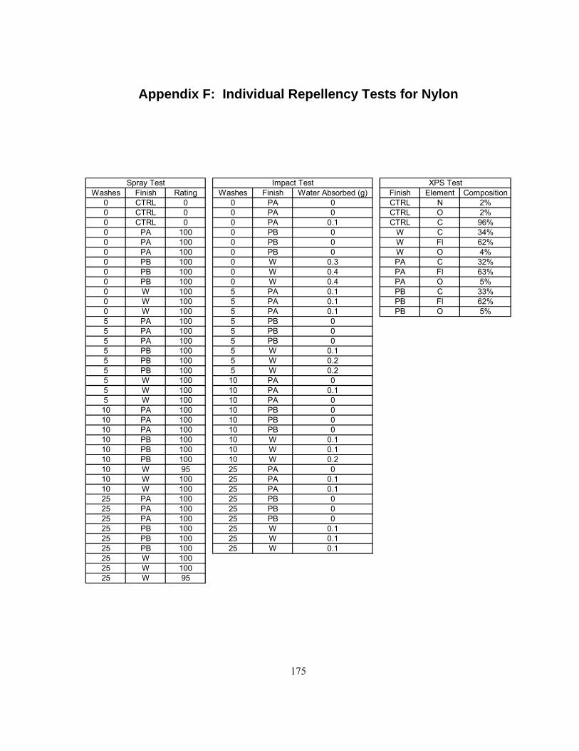
175
Appendix F: Individual Repellency Tests for Nylon
Washes Finish Rating Washes Finish Water Absorbed (g) Finish Element Composition0 CTRL 0 0 PA 0 CTRL N 2%0 CTRL 0 0 PA 0 CTRL O 2%0 CTRL 0 0 PA 0.1 CTRL C 96%0 PA 100 0 PB 0 W C 34%0 PA 100 0 PB 0 W Fl 62%0 PA 100 0 PB 0 W O 4%0 PB 100 0 W 0.3 PA C 32%0 PB 100 0 W 0.4 PA Fl 63%0 PB 100 0 W 0.4 PA O 5%0 W 100 5 PA 0.1 PB C 33%0 W 100 5 PA 0.1 PB Fl 62%0 W 100 5 PA 0.1 PB O 5%5 PA 100 5 PB 05 PA 100 5 PB 05 PA 100 5 PB 05 PB 100 5 W 0.15 PB 100 5 W 0.25 PB 100 5 W 0.25 W 100 10 PA 05 W 100 10 PA 0.15 W 100 10 PA 010 PA 100 10 PB 010 PA 100 10 PB 010 PA 100 10 PB 010 PB 100 10 W 0.110 PB 100 10 W 0.110 PB 100 10 W 0.210 W 95 25 PA 010 W 100 25 PA 0.110 W 100 25 PA 0.125 PA 100 25 PB 025 PA 100 25 PB 025 PA 100 25 PB 025 PB 100 25 W 0.125 PB 100 25 W 0.125 PB 100 25 W 0.125 W 10025 W 10025 W 95
Spray Test Impact Test XPS Test

176
Appendix F: Individual Repellency Tests for Nylon (cont.)
Contact Angle Washes Finish Contact Angle Washes Finish Contact Angle
0 PA 150 10 PA 156 0 PA 143 10 PA 145 0 PA 151 10 PA 151 0 PA 145 10 PA 151 0 PA 145 10 PA 146 0 PB 138 10 PB 151 0 PB 143 10 PB 147 0 PB 148 10 PB 154 0 PB 147 10 PB 158 0 PB 142 10 PB 145 0 W 149 10 W 147 0 W 143 10 W 142 0 W 153 10 W 141 0 W 154 10 W 143 0 W 158 10 W 150 5 PA 144 25 PA 145 5 PA 150 25 PA 152 5 PA 146 25 PA 134 5 PA 149 25 PA 138 5 PA 146 25 PA 142 5 PB 149 25 PB 145 5 PB 153 25 PB 148 5 PB 153 25 PB 143 5 PB 148 25 PB 143 5 PB 152 25 PB 142 5 W 140 25 W 132 5 W 142 25 W 140 5 W 144 25 W 149 5 W 151 25 W 155 5 W 144 25 W 145

177
Appendix F: Contact Angle ANOVA between Finishes (Nylon) As Received
130
135
140
145
150
155
160co
ntac
t ang
le
PA PB W
finish
RsquareAdj RsquareRoot Mean Square ErrorMean of ResponseObservations (or Sum Wgts)
0.3873030.2851864.501851147.2667
15
Summary of Fit
finishErrorC. Total
Source2
1214
DF153.73333243.20000396.93333
Sum of Squares76.866720.2667
Mean Square3.7928F Ratio
0.0529Prob > F
Analysis of Variance
PAPBW
Level555
Number146.800143.600151.400
Mean2.01332.01332.0133
Std Error142.41139.21147.01
Lower 95%151.19147.99155.79
Upper 95%
Std Error uses a pooled estimate of error variance
Means for Oneway Anova
Oneway Anova
Oneway Analysis of contact angle By finish washes=0
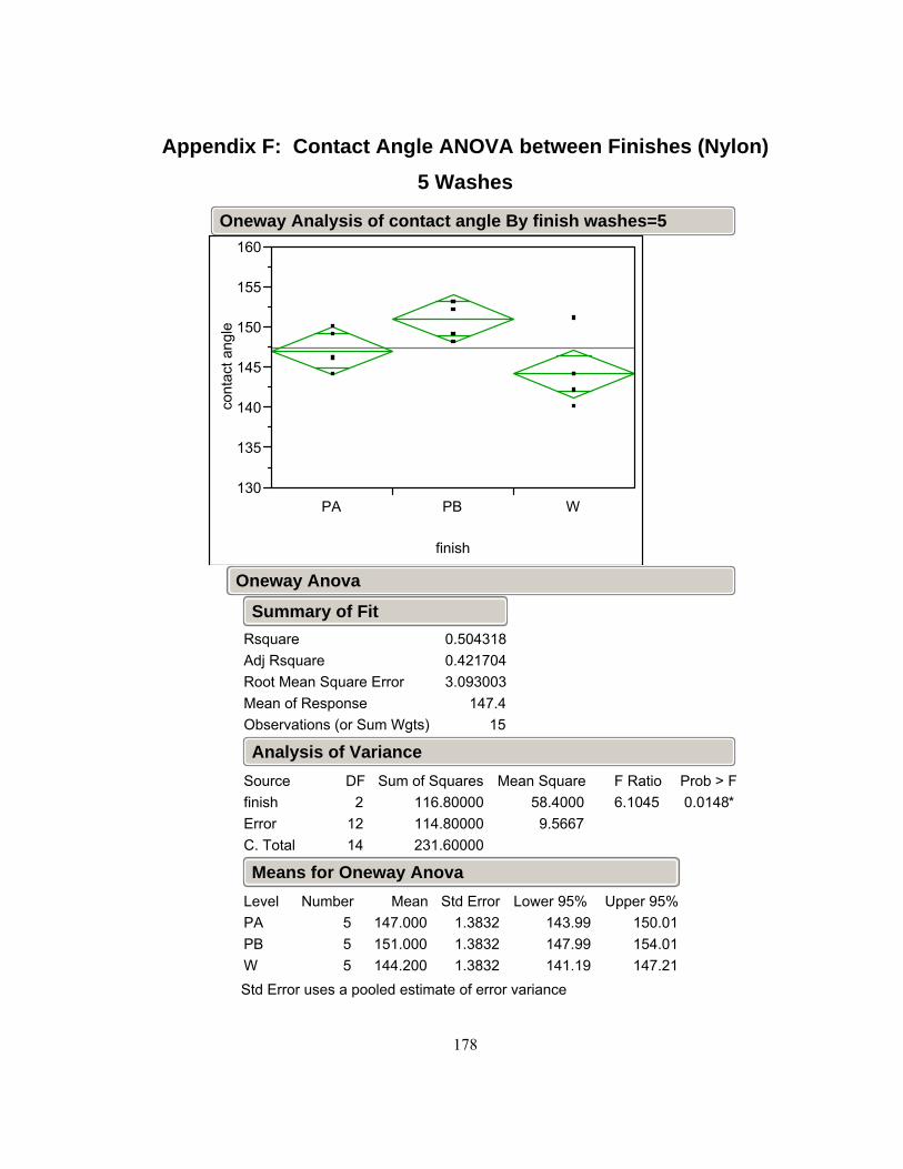
178
Appendix F: Contact Angle ANOVA between Finishes (Nylon) 5 Washes
130
135
140
145
150
155
160co
ntac
t ang
le
PA PB W
finish
RsquareAdj RsquareRoot Mean Square ErrorMean of ResponseObservations (or Sum Wgts)
0.5043180.4217043.093003
147.415
Summary of Fit
finishErrorC. Total
Source2
1214
DF116.80000114.80000231.60000
Sum of Squares58.40009.5667
Mean Square6.1045F Ratio
0.0148*Prob > F
Analysis of Variance
PAPBW
Level555
Number147.000151.000144.200
Mean1.38321.38321.3832
Std Error143.99147.99141.19
Lower 95%150.01154.01147.21
Upper 95%
Std Error uses a pooled estimate of error variance
Means for Oneway Anova
Oneway Anova
Oneway Analysis of contact angle By finish washes=5
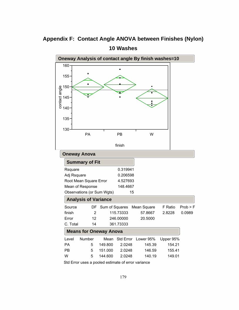
179
Appendix F: Contact Angle ANOVA between Finishes (Nylon) 10 Washes
130
135
140
145
150
155
160co
ntac
t ang
le
PA PB W
finish
RsquareAdj RsquareRoot Mean Square ErrorMean of ResponseObservations (or Sum Wgts)
0.3199410.2065984.527693148.4667
15
Summary of Fit
finishErrorC. Total
Source2
1214
DF115.73333246.00000361.73333
Sum of Squares57.866720.5000
Mean Square2.8228F Ratio
0.0989Prob > F
Analysis of Variance
PAPBW
Level555
Number149.800151.000144.600
Mean2.02482.02482.0248
Std Error145.39146.59140.19
Lower 95%154.21155.41149.01
Upper 95%
Std Error uses a pooled estimate of error variance
Means for Oneway Anova
Oneway Anova
Oneway Analysis of contact angle By finish washes=10

180
Appendix F: Contact Angle ANOVA between Finishes (Nylon) 25 Washes
130
135
140
145
150
155
160co
ntac
t ang
le
PA PB W
finish
RsquareAdj RsquareRoot Mean Square ErrorMean of ResponseObservations (or Sum Wgts)
0.025075-0.137416.572671143.5333
15
Summary of Fit
finishErrorC. Total
Source2
1214
DF13.33333
518.40000531.73333
Sum of Squares6.6667
43.2000
Mean Square0.1543F Ratio
0.8587Prob > F
Analysis of Variance
PAPBW
Level555
Number142.200144.200144.200
Mean2.93942.93942.9394
Std Error135.80137.80137.80
Lower 95%148.60150.60150.60
Upper 95%
Std Error uses a pooled estimate of error variance
Means for Oneway Anova
Oneway Anova
Oneway Analysis of contact angle By finish washes=25

181
Appendix F: Contact Angle ANOVA Within Finishes (Nylon) Conventional (W) Finish
130
135
140
145
150
155
160
cont
act a
ngle
0 5 10 25
washes
RsquareAdj RsquareRoot Mean Square ErrorMean of ResponseObservations (or Sum Wgts)
0.2504670.1099295.926635
146.120
Summary of Fit
washesErrorC. Total
Source3
1619
DF187.80000562.00000749.80000
Sum of Squares62.600035.1250
Mean Square1.7822F Ratio
0.1911Prob > F
Analysis of Variance
051025
Level5555
Number151.400144.200144.600144.200
Mean2.65052.65052.65052.6505
Std Error145.78138.58138.98138.58
Lower 95%157.02149.82150.22149.82
Upper 95%
Std Error uses a pooled estimate of error variance
Means for Oneway Anova
Oneway Anova
Oneway Analysis of contact angle By washes finish=W

182
Appendix F: Contact Angle ANOVA Within Finishes (Nylon) First Plasma (PA) Finish
130
135
140
145
150
155
160co
ntac
t ang
le
0 5 10 25
washes
RsquareAdj RsquareRoot Mean Square ErrorMean of ResponseObservations (or Sum Wgts)
0.3038140.1732794.612483
146.4520
Summary of Fit
washesErrorC. Total
Source3
1619
DF148.55000340.40000488.95000
Sum of Squares49.516721.2750
Mean Square2.3275F Ratio
0.1133Prob > F
Analysis of Variance
051025
Level5555
Number146.800147.000149.800142.200
Mean2.06282.06282.06282.0628
Std Error142.43142.63145.43137.83
Lower 95%151.17151.37154.17146.57
Upper 95%
Std Error uses a pooled estimate of error variance
Means for Oneway Anova
Oneway Anova
Oneway Analysis of contact angle By washes finish=PA

183
Appendix F: Contact Angle ANOVA Within Finishes (Nylon) Second Plasma (PB) Finish
130
135
140
145
150
155
160co
ntac
t ang
le
0 5 10 25
washes
RsquareAdj RsquareRoot Mean Square ErrorMean of ResponseObservations (or Sum Wgts)
0.5348350.4476163.708099
147.4520
Summary of Fit
washesErrorC. Total
Source3
1619
DF252.95000220.00000472.95000
Sum of Squares84.316713.7500
Mean Square6.1321F Ratio
0.0056*Prob > F
Analysis of Variance
051025
Level5555
Number143.600151.000151.000144.200
Mean1.65831.65831.65831.6583
Std Error140.08147.48147.48140.68
Lower 95%147.12154.52154.52147.72
Upper 95%
Std Error uses a pooled estimate of error variance
Means for Oneway Anova
Oneway Anova
Oneway Analysis of contact angle By washes finish=PB
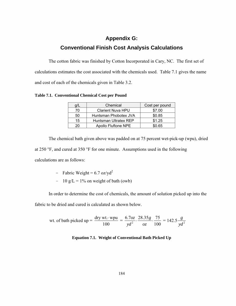
184
Appendix G: Conventional Finish Cost Analysis Calculations
The cotton fabric was finished by Cotton Incorporated in Cary, NC. The first set of
calculations estimates the cost associated with the chemicals used. Table 7.1 gives the name
and cost of each of the chemicals given in Table 3.2.
Table 7.1. Conventional Chemical Cost per Pound
g/L Chemical Cost per pound 70 Clarient Nuva HPU $7.00 50 Huntsman Phobotex JVA $0.85 15 Huntsman Ultratex REP $1.25 20 Apollo Fluftone NPE $0.65
The chemical bath given above was padded on at 75 percent wet-pick-up (wpu), dried
at 250 °F, and cured at 350 °F for one minute. Assumptions used in the following
calculations are as follows:
- Fabric Weight = 6.7 oz/yd2
- 10 g/L = 1% on weight of bath (owb)
In order to determine the cost of chemicals, the amount of solution picked up into the
fabric to be dried and cured is calculated as shown below.
2 2
dry wt. wpu 6.7 28.35 75wt. of bath picked up = = = 142.5100 100
oz g gyd oz yd
⋅⋅ ⋅
Equation 7.1. Weight of Conventional Bath Picked Up

185
Although the weight of the bath picked up was 142.5 grams per square yard, much of
it was water. In order to determine the amount of chemicals in the bath, it was assumed that
10 g/L of chemical is 1% owb. There was a total of 155 g/L of chemicals added to the bath;
therefore, 15.5% of the 142.5 g/yd2 of bath picked up were the chemicals in Table 7.1. The
amount of chemicals picked up by the bath after padding to be dried and cured is given
below.
2 2chemicals picked up = 142.5 15.5% = 22.1g gyd y
⋅d
Equation 7.2. Conventional Chemicals Picked Up
Since the amount of chemicals picked up was determined, they were broken down
into the individual chemicals given in Table 7.1 in order to determine the costs for each
chemical. This is calculated on the following page in Equation 7.3.

186
2
2
2
70 $7 $0.15Clarient Nuva HPU: 22.1454155
50 $0.85 $0.013Huntsman Phobotex JVA: 22.1454155
15 $1.25 $0.0059Huntsman Ultratex RFP: 22.1454155
Apollo Flu
gg lbL
g L lb g ydL
gg lbL
g L lb g ydL
gg lbL
g L lb g ydL
⋅ ⋅ ⋅ =
⋅ ⋅ ⋅ =
⋅ ⋅ ⋅ =
2
20 $0.65 $0.0041fftone NPE: 22.1454155
gg lbL
g L lb g ydL
⋅ ⋅ ⋅ =
2
$0.18(chemical cost) = yd∑
Equation 7.3. Conventional Chemical Cost
To determine the energy cost associated with the drying and curing process,
American Monforts was contacted. American Monforts is a large company specializing in
supplying tenter machines to the textile industry and they agreed to determine the energy
consumption that would be required to dry and cure the cotton fabric with the chemical bath
as described above. Table 7.2 on the following page shows the variables that were used by
American Monforts in order to determine the energy consumption.

187
Table 7.2. Information Used by American Monforts
Fabric Type 100% Cotton Fabric Weight 6.7 oz/sq yd Fabric Width 65 inches
Desired Speed 25 yards/minute Dry at 350 deg. F
Cure at 350 deg. F for 1 min
The results returned from American Monforts are given below in Table 7.3. The
energy consumption results are in a ± 10 percent tolerance.
Table 7.3. Information Returned by American Monforts
Machine Montex-TwinAir Stenter, 10 zones Actual Speed 24 yards/min
Heat Energy without Heat Recovery 1405861 BTU/hr Heat Requirement per kg Evaporated H20 3056 BTU/kg H20
Total Electrical Power 224 KW
With the total amount of energy consumed by a tenter known, the energy costs can be
calculated. It will be assumed that the energy required to cure the chemicals is negligible
compared to the energy required to evaporate water. In addition, the following assumptions
will be made to determine energy cost.
- Electricity costs = $0.1265/KWh
- Natural Gas costs = $7.85/MMBTU
Equation 7.4 was used to determine the cost of electricity to power the tenter.
2
Electricity Cost $0.1265Power 224 $0.01160 60=Width Speed 65 24
36
hr KWKW hr min
yd yds ydinin min
⋅ ⋅ ⋅⋅ =
⋅ ⋅ ⋅

188
Equation 7.4. Tenter Electricity Cost
To determine the cost to dry and cure the fabric, the energy required to heat the tenter
and the energy to dry and cure the fabric will be calculated separately. Equation 7.5 below
was used to calculate how much it costs to use natural gas to keep a tenter at a set 350 °F.
6 2
1, 405,861$7.85 $0.004260
1065 2436
BTU hrhr min
yd yds BTU ydinin min
⋅⋅ =
⋅ ⋅
Equation 7.5. Natural Gas Cost to Maintain Tenter at 350 °F
Equation 7.6 was used to determine the cost associated with drying and curing the
amount of bath that was picked up as calculated in Equation 7.1.
2 6
142.5 3,056 $7.85 $0.00341000 10
g kg BTUyd g kg BTU yd
⋅ ⋅ ⋅ = 2
Equation 7.6. Natural Gas Cost to Dry and Cure
Equation 7.5 and Equation 7.6 result in the total cost of natural gas per square yard of
fabric to be $0.0077. These results suggest that it costs $0.20 per square yard to treat a fabric
with the conventional pad-dry-cure finish.

189
Appendix H: APPLD Cost Analysis Calculations
The following calculations were used to determine the approximate costs associated
with the APPLD process. There are three main costs linked with the APPLD treatment:
process gas, chemical precursors used, and electricity. The chemical cost will obviously be
the most expensive because the precursor chemicals used in this research were specialty
monomers. For this reason, multiple chemical vendors were contacted to determine a bulk
rate.
Out of five requests sent to different chemical manufacturers for each chemical, there
was only one response. A Chinese company called Feiyang provided a quote for the
HDFDA at 99.95 USD per kilogram for a 500 pound minimum order not including any
shipping charges. Because there was no response from any of the chemical vendors
contacted regarding a bulk price for the HDFD, the HDFD price was estimated by using the
same ratio as the HDFDA’s research to bulk price.
Table 7.4. Price of Chemical Precursors
Chemical CAS # Density (g/mL) Research Price Bulk Price HDFD 21652-58-4 1.67 $24.8 for 5 grams *$23.33 per lb
HDFDA 27905-45-9 1.64 $48.3 for 5 grams $45.43 per lb * estimated from HDFDA
The following calculations will determine the total cost associated with the APPLD
process used in this research. The APPLD settings from Table 4.2 will be used for the
following calculations along with the assumptions below.

190
- Electricity costs = $0.1265/KWh
- Helium costs = $0.0198/L
The calculations below determine the cost of electricity and helium in the APPLD
process.
2
Electricity Cost $0.1265Power 1.8 $0.006260 60#Passes= 35Width Speed 1236
hr KWKW hr min
yd m yds ydinin min 0.91m
⋅ ⋅ ⋅⋅⋅ ⋅
⋅ ⋅ ⋅ ⋅=
Equation 7.7. APPLD Electricity Cost
2
Total He Flow $He 25 / $0.0198 $0.81#Passes = 35Width SpeedL min
yd m ydsL L yd12in36 in min 0.91m
⋅ ⋅ ⋅ ⋅ =⋅ ⋅ ⋅ ⋅
Equation 7.8. APPLD Helium Cost
Next, the total cost of the chemical precursors used in the APPLD process was
calculated. This calculation contained three steps. The first step was to determine the total
mass of the chemical precursors that are injected into the plasma every minute as given in
Equation 7.9. Then the total mass of the precursors that was injected into the plasma region
per minute was converted to the total mass of precursors that polymerized on the surface of
the fabric per square yard, assuming 100 percent efficiency as shown in Equation 7.10.
Lastly, the amount of chemical precursors used was multiplied by the bulk cost of the
chemicals to determine the cost of chemical precursors per square yard of fabric.

191
The mass of the precursors that were injected into the plasma region per minute was
calculated by taking the total flow of each precursor and multiplying it by its density. The
precursors used in this research were a 50:50 blend by volume.
1.5 1.67 50 1.5 1.64 50 1.25 1.23HDFD HDFDA HDFD HDFDAmL g mL g g g% %
min mL min mL min min⎛ ⎞ ⎛ ⎞⋅ ⋅ + ⋅ ⋅ = +⎜ ⎟ ⎜ ⎟⎝ ⎠ ⎝ ⎠
Equation 7.9. Mass of Precursor Injected into Plasma Region
2 2
1.25 1.233 3 2.06 2.02
12 5.47 12 5.4736 36
HDFD HDFDA
HDFD HDFDAg g
g gmin minpasses passesyd yds yd yds yd ydin inin min in min
⋅ + ⋅ = +⋅ ⋅ ⋅ ⋅
Equation 7.10. Mass of Precursor on Fabric
2 2 2
$23.33 $45.43 $0.11 $0.202.06 2.02454 454
HDFD HDFDA HDFD HDFDAg lb g lb
yd g lb yd g lb yd yd⎛ ⎞ ⎛ ⎞ ⎛ ⎞ ⎛
⋅ ⋅ + ⋅ ⋅ = +⎜ ⎟ ⎜ ⎟ ⎜ ⎟ ⎜⎝ ⎠ ⎝ ⎠ ⎝ ⎠ ⎝
2
⎞⎟⎠
Equation 7.11 . Cost of Chemical Precursors
The results from the above calculations show that the chemicals used in this research
costs $0.31 per square yard. This results in the total cost per square yard of fabric tested in
this research at $1.13.
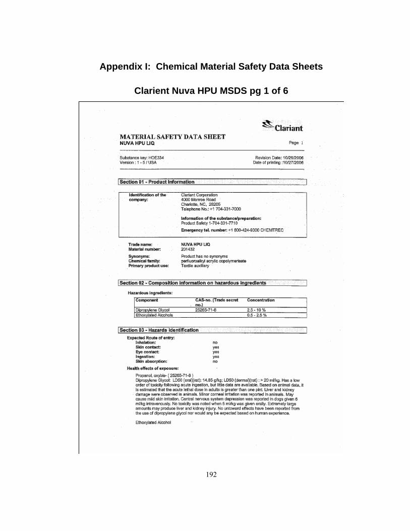
192
Appendix I: Chemical Material Safety Data Sheets
Clarient Nuva HPU MSDS pg 1 of 6

193
Appendix I: Clarient Nuva HPU MSDS pg 2 of 6

194
Appendix I: Clarient Nuva HPU MSDS pg 3 of 6

195
Appendix I: Clarient Nuva HPU MSDS pg 4 of 6

196
Appendix I: Clarient Nuva HPU MSDS pg 5 of 6
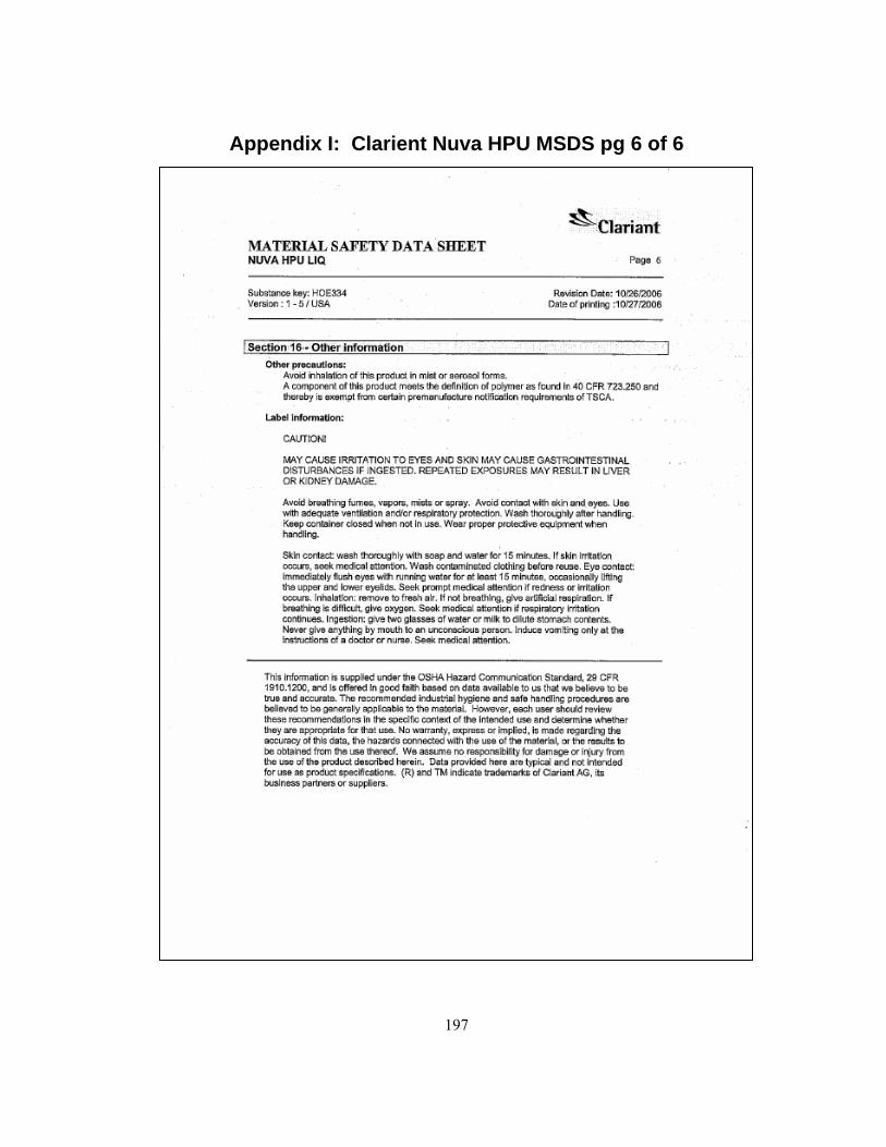
197
Appendix I: Clarient Nuva HPU MSDS pg 6 of 6
198
Appendix I: Huntsman Phobotex JVA MSDS pg 1 of 7

199
Appendix I: Huntsman Phobotex JVA MSDS pg 2 of 7

200
Appendix I: Huntsman Phobotex JVA MSDS pg 3 of 7

201
Appendix I: Huntsman Phobotex JVA MSDS pg 4 of 7

202
Appendix I: Huntsman Phobotex JVA MSDS pg 5 of 7

203
Appendix I: Huntsman Phobotex JVA MSDS pg 6 of 7
204
Appendix I: Huntsman Phobotex JVA MSDS pg 7 of 7

205
Appendix I: Huntsman Ultratex REP MSDS pg 1 of 6

206
Appendix I: Huntsman Ultratex REP MSDS pg 2 of 6

207
Appendix I: Huntsman Ultratex REP MSDS pg 3 of 6
208
Appendix I: Huntsman Ultratex REP MSDS pg 4 of 6

209
Appendix I: Huntsman Ultratex REP MSDS pg 5 of 6

210
Appendix I: Huntsman Ultratex REP MSDS pg 6 of 6

211
Appendix I: Apollo Fluftone NPE MSDS pg 1 of 4

212
Appendix I: Apollo Fluftone NPE MSDS pg 2 of 4

213
Appendix I: Apollo Fluftone NPE MSDS pg 3 of 4

214
Appendix I: Apollo Fluftone NPE MSDS pg 4 of 4

215
Appendix I: HDFDA MSDS pg 1 of 6

216
Appendix I: HDFDA MSDS pg 2 of 6

217
Appendix I: HDFDA MSDS pg 3 of 6
218
Appendix I: HDFDA MSDS pg 4 of 6

219
Appendix I: HDFDA MSDS pg 5 of 6
220
Appendix I: HDFDA MSDS pg 6 of 6

221
Appendix I: HDFD MSDS pg 1 of 4

222
Appendix I: HDFD MSDS pg 2 of 4

223
Appendix I: HDFD MSDS pg 3 of 4

224
Appendix I: HDFD MSDS pg 4 of 4


