

7
TSE‐885
“FinancialIntermediation,CapitalAccumulationandCrisis
Recovery”
HansGersbach,Jean‐CharlesRochetandMartinScheffel
January 2018

Financial Intermediation, Capital Accumulation and
Crisis Recovery∗
Hans Gersbach
CER-ETH – Center of Economic
Research at ETH Zurich and CEPR
Zurichbergstrasse 18
8092 Zurich, Switzerland
Jean-Charles Rochet
Swiss Finance Institute
at University of Zurich,
University of Geneva and
Toulouse School of Economics
Martin Scheffel
Center for Macroeconomic Research
University of Cologne and
Department of Economics
University of Mannheim
This Version: November 2017
Abstract
This paper integrates banks into a two-sector neoclassical growth model to account for
the fact that a fraction of firms relies on banks to finance their investments. There are
four major contributions to the literature: First, although banks’ leverage amplifies shocks,
the endogenous response of leverage to shocks is an automatic stabilizer that improves the
resilience of the economy. In particular, financial and labor market institutions are essential
factors that determine the strength of this automatic stabilization. Second, there is a mix
of publicly financed bank re-capitalization, dividend payout restrictions, and consumption
taxes that stimulates a Pareto-improving rapid build-up of bank equity and accelerates
economic recovery after a slump in the banking sector. Third, the model replicates typical
patterns of financing over the business cycle: procyclical bank leverage, procyclical bank
lending, and countercyclical bond financing. Fourth, the framework preserves its analytical
tractability wherefore it can serve as a macro-banking module that can be easily integrated
into more complex economic environments.
JEL: E21, E32, F44, G21, G28
Keywords: Financial intermediation, capital accumulation, banking crisis, macroe-
conomic shocks, business cycles, bust-boom cycles, managing recoveries.
∗We would like to thank Tobias Adrian, Phil Dybvig, Tore Ellingsen, Salomon Faure, Mark Flannery,Douglas Gale, Gerhard Illing, Pete Kyle, Dalia Marin, Joao Santos, Klaus Schmidt, Maik Schneider, UweSunde and seminar participants at ETH Zurich, the European University Institute, Imperial College,the Bank of Korea, the University of Munich, the Federal Reserve Bank of New York, Oxford University,and the Stockholm School of Economics for valuable comments. We are particularly grateful to MichaelKrause for detailed suggestions how to improve the paper. Jean-Charles Rochet acknowledges financialsupport from the Swiss Finance Institute and the European Research Council (Grant Agreement 249415).

1 Introduction
Financial frictions affect the propagation of economic shocks and are an essential factor
for understanding short-run dynamics and long-run macroeconomic performance. Typi-
cally, financial frictions can be traced back to either contract enforceability problems or
asymmetric information and – on this ground – give rise to levered finance to align the
interest of borrowers and lenders.1
Since the seminal contributions of Bernanke and Gertler (1989), Bernanke et al. (1996)
and Kiyotaki and Moore (1997), it is well-understood that in an economy with financial
frictions, even small temporary shocks can have large and persistent effects on economic
activity by impacting the net worth of levered agents. In this literature, firms need
net worth to credibly commit to the contractual obligations of the credit contract. De-
teriorating conditions reduce firm profits, net worth and, thus, the capacity to obtain
credit. The propagation of shocks through net worth and firm credit may have large and
persistent impact on economic activity – a mechanism referred to as the credit channel.2
Although Holmstrom and Tirole (1997) extended the analysis to financial intermediaries,
it was not until the 2007-2009 financial and banking crisis that macroeconomists took up
their proposal. Financial intermediaries channel funds from investors to entrepreneurs,
cope with the underlying financial friction and are, at the same time, subject to frictions
themselves. Banks have to hold equity capital to credibly commit to the contractual
obligations of the deposit contract. Specifically, the level of bank equity is the skin
in the game which determines the capacity to attract loanable funds. When financial
conditions deteriorate, bank profits decline, which negatively affects future bank equity
holdings and, thus, the future capacity to attract loanable funds and to supply loans to
entrepreneurs. The propagation of shocks through the bank balance sheets has real large
and persistent impact on economic activity – a mechanism referred to as the bank lending
channel.3 In essence, the bank lending channel is a propagation mechanism similar to
the credit channel, but it impacts different borrowers.4
In this paper, we develop a two-sector neoclassical growth model with financial frictions
in the tradition of Holmstrom and Tirole (1997). The model has microfounded levered
1See Quadrini (2011) for an excellent overview of the extensive literature on financial frictions andmacroeconomic performance.
2This literature includes Carlstrom and Fuerst (1997) and, more recently, Cooley et al. (2004),Christiano et al. (2007), Jermann and Quadrini (2012), Brumm et al. (2015), and Gomes et al. (2016).
3This literature includes Van den Heuvel (2008), Meh and Moran (2010), Gertler and Kiyotaki (2010),Gertler and Karadi (2011), Rampini and Viswanathan (2017), Brunnermeier and Sannikov (2014), andQuadrini (2014).
4There are also notable deviations from this approach to model banking systems in macroeconomiccontext, see e.g. Angeloni and Faia (2013) and Acemoglu et al. (2015).
1

banks and allows for two forms of finance – bonds and loans. We adopt a medium-
to long-run perspective in the sense that output reacts smoothly to adverse shocks
and economic dynamics are essentially driven by capital re-allocation and accumulation
instead of abrupt changes in prices. We contribute to the literature in four respects.
First, we provide novel insights into the bank lending channel. We show that although
the level of leverage is an amplification mechanism of shocks, the endogenous response
of leverage to productivity and capital shocks is an automatic stabilizer that improves
the resilience of the economy to adverse shocks. Specifically, suppose there is a shock
that – directly or indirectly – leads to a decline in bank equity. Investors, ceteris paribus,
reduce their deposits to restore the initial bank leverage, i.e. loan supply decreases. As a
result, capital productivity in the loan financed sector increases and so do bank profits.
The effective financial friction loosens such that investors can increase their deposits
without incentivizing banks to defect. The ensuing increase in bank leverage partially
neutralizes the initial decline in loan supply.
In particular, we show that financial market institutions (e.g. capital requirements) and
labor market institutions (e.g. labor mobility and employment protection legislation)
affect the elasticity of bank leverage with respect to productivity and capital shocks
and, therefore, the resilience of the financial system. While the impact of financial
market institutions on labor markets is well-understood, we show that there is a non-
negligible feedback effect from labor market institutions to credit market conditions
and the resilience of the financial system – a result unique to the macro-banking and
macro-labor literature.
Second, we derive macro-prudential policies comprising investor-financed re-capitalization
of banks, dividend payout restrictions, consumption taxes, and investment subsidies that
are Pareto-improving and speed up the economic recovery after a banking crisis, without
encouraging banks to take excessive leverage in the expectations of future bailouts. In a
similar vein, Acharya et al. (2017) show that bank equity capital has the characteristics
of a public good which justifies dividend pay-out restrictions to internalize the impact
of dividend payments on social welfare and output. In fact, bank-recapitalization and
dividend pay-out restrictions have been used during the 2007 – 2009 financial and bank-
ing crisis in the United States and, as Shin (2016) points out, during the 2007 – 2014
financial and banking crisis in Europe.
Third, the model replicates typical patterns of financing over the business cycle: pro-
cyclical bank leverage, procyclical bank lending and countercyclical bond financing –
see Adrian and Shin (2014), Adrian and Boyarchenko (2012), Adrian and Boyarchenko
(2013) and Nuno and Thomas (2012) for empirical evidence. This holds if downturns are
associated with negative productivity, bank equity or trust shocks – or any combination
2

thereof. Moreover, when recessions are accompanied by a sharp temporary decline in
bank equity capital, they are deeper and more persistent than regular recessions – a
result that is consistent with the findings in Bordo et al. (2001), Allen and Gale (2009),
and Schularick and Taylor (2012).
Fourth, our model provides an analytically tractable macro-banking module that can
easily be integrated into more complex economic environments to give more account for
the special roles of banks in macroeconomic analysis.
Financial frictions are at the core of our macro-banking model: they provide a micro-
foundation for the existence of banks and play an essential role for the propagation of
adverse shocks.5 Specifically, there are two production sectors. Firms in sector I (in-
termediary financed) are subject to severe financial frictions, which prevents them from
obtaining financing directly through the financial market. As banks alleviate the moral
hazard problems resulting from these financial frictions, firms in sector I obtain bank
loans instead. However, bank lending itself is limited, as bankers can only pledge a frac-
tion of their revenues to depositors and are thus subject to a different financial friction
that gives rise to an endogenous leverage constraint which depends on equilibrium cap-
ital returns in sector I and the deposit rate. Firms in sector M (market financed) are
not subject to financial frictions and issue corporate bonds. The need for bank lending
– also called informed lending – coupled with the lack of full revenue pledgeability, are
the two financial frictions in our model.6 In the baseline model, there are three types
of agents: investors, bankers and workers. The latter are immobile across production
sectors as their skills are sector-specific. Workers do not save and consume their entire
labor income. Investors and bankers have standard intertemporal preferences and decide
in each period how much to save and to consume.7 Their utility maximization problems
yield two accumulation rules for investor wealth and bank equity, respectively. These
rules are coupled in the sense that the investor’s saving and investment policies depend
on how bankers fare and vice versa. Both types of lending – informed lending by banks
and uninformed lending through capital markets – enable capital accumulation in the
respective sectors.
The paper is organized as follows. Section 2 relates our paper to the existing literature.
5Gersbach and Rochet (2017) study a static version of the same banking model in which bank equitycapital cannot be accumulated. Gersbach et al. (2016) integrate banks into the Solow growth model.
6As we discuss in Section 3.3, the foundation of these frictions can be moral hazard problems a laHolmstrom and Tirole (1997), asset diversion (as in Gertler and Karadi (2011) and Gertler and Kiyotaki(2010)) or non-alienability of human capital (as in Hart and Moore (1994) and Diamond and Rajan(2000)).
7In the extensions, we consider a version of the model in which there are only two types of agents:households, acting as investors and workers, and banks. To preserve clarity in exposition, we solely usethe terminus household for that case.
3

Section 3 introduces the model, Section 4 defines and characterizes sequential market
equilibria, and Section 5 analyzes the steady state allocation. Section 6 establishes
global stability, characterizes global economic dynamics, and analyzes the propagation
of adverse shocks when bank leverage reacts sensitive to equilibrium conditions. Section 7
derives public policies and financial regulation to speed up recoveries when the economy is
hit by a negative shock to bank equity capital. Section 8 provides a quantitative analysis
to illustrate the static and dynamic effects that have been derived in the previous sections
of this paper. Section 9 summarizes and concludes. Several extensions to the model are
relegated to Appendix D.
2 Relation to the Literature
Our paper is closely related to three recent strands of the literature that integrate fi-
nancial intermediation into macroeconomic models. The objective is to analyze the
propagation of shocks through bank balance sheets and to derive policies to manage
financial and banking crises.
First, our paper is most closely related to recent research that integrates financial inter-
mediation into the neoclassical growth model, e.g. Van den Heuvel (2008), Gertler and
Kiyotaki (2010), Rampini and Viswanathan (2017), Brunnermeier and Sannikov (2014),
Quadrini (2014), and Acemoglu et al. (2015). Brunnermeier and Sannikov (2014) have
stressed that the economy’s reaction to adverse shocks can be highly non-linear. Specif-
ically, if the economy is sufficiently far away from its steady state, even small shocks
can generate substantial amplification and endogenous fluctuations. In contrast, near
the steady state, the economy is resilient to most shocks. He and Krishnamurthy (2013)
find similar non-linear effects when risk premia on equity increase sharply as finan-
cial constraints become binding. Rampini and Viswanathan (2017) develop a dynamic
theory of financial intermediaries acting as collateralization specialists, in which credit
crunches are persistent and can delay or stall economic recoveries. They consider a
one-sector economy with risk-neutral agents and show that – under certain conditions
– there are large reactions to small changes in interest rates. In contrast to Rampini
and Viswanathan (2017), we develop a two-sector neoclassical growth model with lev-
ered financial intermediation where savings, investments, interest rates, and bank capital
accumulation react more smoothly to shocks for three reasons:
First, with an alternative investment opportunity that does not rely on levered finance,
investors re-optimize their portfolio, thereby attenuating the immediate impact of an ad-
verse shock. Second, as investors are risk-averse, they smooth consumption and spread
the immediate shock to several periods. Third, leverage itself reacts endogenously and
4

immediately accommodates the banks’ lending capacity to smooth out adverse shocks
to the bank balance sheet. Nevertheless, the special role of banks in the capital accu-
mulation process with binding leverage constraints as well as the potentially divergent
reactions of investor wealth and bank equity capital generate sizeable and persistent
output reactions, as bank profits and thus future lending capacities are affected. In
this sense, our approach adopts a medium- to long-run perspective on how economies
with a large bank-financed sector react to shocks, because economic dynamics are driven
by adjustments in capital accumulation instead of abrupt changes in price levels. An-
other difference with Rampini and Viswanathan (2017) is that in our model, the relative
capital productivity of financially constrained and unconstrained firms is endogenously
determined by the joint evolution of bank equity and investor capital. The mix of bond
and loan finance evolves endogenously and replicates typical financing patterns over
the business cycle: counter-cyclical bond-to-loan finance ratios (see De Fiore and Uhlig
(2011)) and pro-cyclical bank leverage (see Adrian and Shin (2014)). In addition, an
increase of the financial frictions induces a recession in the economy, but leads to a boom
in the banking sector that can – under certain conditions – even trigger a boom in the
economy in the medium-run.
Second, our paper is closely related to a recent strand in the literature that integrates
banks into New-Keynesian DSGE models, e.g. Meh and Moran (2010), Gertler and
Karadi (2011), and Angeloni and Faia (2013). Meh and Moran (2010) and Angeloni
and Faia (2013) have provided valuable insights about the bank capital transmission
channel. Meh and Moran (2010) find that this channel amplifies the impact of technology
shocks on inflation and output, and delays economic recovery. Angeloni and Faia (2013)
introduce a fragile banking system, in which banks are subject to runs, into a new-
Keynesian DSGE model. They show that a combination of counter-cyclical capital
requirements and monetary policies responding to asset prices or bank leverage is optimal
in the sense that it maximizes the ex-ante expected value of total payments to depositors
and bank capitalists. In contrast to this strand of literature, we abstract from price
rigidities and develop a parsimonious neoclassical macro-banking model that exhibits
smooth reactions to adverse shocks. In contrast to Angeloni and Faia (2013), we focus
on incentive compatible ex-post policies to manage financial and banking crises instead
of ex-ante policies to prevent them.
Third, in terms of policy implications, our paper is closely related to Martinez-Miera and
Suarez (2012), who study a dynamic general equilibrium model in which banks decide
inter alia on their exposure to systemic shocks. Capital requirements reduce the direct
impact of negative systemic shocks, but they also lower credit supply and output in
normal times: optimal capital requirements balance these costs and benefits. Our model
5

is complementary to Martinez-Miera and Suarez (2012) and considers the simultaneous
build-up of bank equity and investor wealth after both, anticipated and unanticipated
shocks to productivity, wealth, and financial frictions. In contrast to Martinez-Miera and
Suarez (2012), who focus on capital requirements and crisis prevention, we focus on crisis
management and show that a revenue-neutral combination of investor-financed bank re-
capitalization, publicly enforced dividend payout restrictions, consumption taxes and
saving subsidies can speed up the recovery after a banking crisis and, in particular, can
make workers and investors better off, while leaving the welfare of bankers unaffected.
In a similar vein, Itskhoki and Moll (2014) study how taxes or subsidies may favorably
impact the transition dynamics in a standard growth model with financial frictions. Our
study is complementary, as we focus on two policies that are typically applied in banking
crises: re-capitalization of banks and dividend payout restrictions. Acharya et al. (2011)
study dividend payments of banks in the 2007 – 2009 financial crisis and argue that early
suspension of dividend payments can prevent the erosion of bank capital in the future.
In a similar vein, Acharya et al. (2017) and Onali (2014) suggest that because dividend
payments exert externalities on other banks, dividend payout restrictions can adjust for
the negative external effect.
3 Model
We integrate a simple model of banks into a two-sector neoclassical growth model. Time
is discrete and denoted by t ∈ 0, 1, 2, . . . . There are two production sectors, with
constant returns to scale technologies using capital and labor to produce a homogenous
good that can be consumed or invested. Sectors differ with respect to their access
to capital markets: while firms in sector M (market-financed or bond-financed) can
borrow frictionlessly on the capital market, firms in sector I (intermediary-financed
or loan-financed) have no direct access to financial markets and rely on bank loans
instead. Banks monitor entrepreneurs in sector I and enforce the contractual obligation
from the loan contract. Banks themselves are subject to financial frictions that limit
the amount of loanable funds these banks can attract. Consumption is the numeraire:
its price is normalized to 1. There are three types of agents: workers, investors, and
bankers.8 Workers are hand-to-mouth consumers who consume their entire labor income
instantaneously. In contrast, investors and bankers choose consumption and investment
8Splitting the household sector into workers and investors preserves the analytical tractability of themodel. We also consider a variation of the model in Section 9 and Appendix D in which there is onlyone type of households that supplies labor and acts as investor. We show that this variation leaves thesteady state allocation unaffected and yields model dynamics that are qualitatively and quantitativelyat a similar order of magnitude.
6

to maximize lifetime utility. The general structure of the model is depicted in Figure 1
and the details are set out in this section.
Figure 1: General Structure of the Model
Firm M Firm I
FM (KM
t, LM
t) F I (KI
t, LI
t)
Workers: LM
t= LM , LI
t= LI
Investors: Ωt = Dt + KI
t
Banks
KI
t
Et
DtKM
tRM
tKM
t
KI
tRI
tKI
t
Dt RD
tDt
LI
twI
tLI
twM
tLM
tLM
t
3.1 Production
Production takes place in two different sectors labeled as sector M and sector I. Both
sectors consist of a continuum of identical firms. The production technologies exhibit
constant returns to scale in the production factors capital and labor, have positive and
diminishing marginal returns regarding a single production factor and satisfy the Inada
conditions. Because of constant returns to scale and competitive markets, we focus on
a price-taking representative producer in each sector, without loss of generality. Specif-
ically, the aggregate production technologies are Cobb-Douglas and given by
Y jt = zjAt
(
Kjt
)α(
Ljt
)1−α, j ∈ M, I,
where At is an index of the economy-wide common total factor productivity, zj is an
index of sectoral total factor productivity, α (0 < α < 1) is the output elasticity of
capital, and Kjt and Lj
t denote capital and labor input in sector j ∈ M, I, respectively.
Firms in sector M can borrow frictionlessly on capital markets by issuing corporate
bonds. Firms in sector I have neither the reputation nor the transparency to resolve
information asymmetries, such that they cannot credibly pledge repayment to investors.
A severe moral hazard problem between investors and firms in sector I ensues, which
leads to the exclusion of the latter from capital markets. These firms, however, can
7

obtain loans from financial intermediaries that monitor them and enforce the contractual
obligation.9 For simplicity, we assume that banks can ensure full repayments of bank
loans.10
Taking interest and wage rates as given, the representative firm in each sector j ∈ M, I
chooses capital and labor to maximize its period profit
maxKj
t ,Ljt
zjAt(
Kjt
)α (
Ljt
)1−α− rj
t Kjt − wj
t Ljt
, j ∈ M, I, (1)
where wjt is the wage rate and rj
t is the rental rate of capital in sector j and period t,
respectively. We further define Kt.= KM
t + KIt and Lt
.= LM
t + LIt as total capital and
total labor used in production.
3.2 Workers and Investors
There is a continuum of workers with mass L (L > 0). Each worker is endowed with
one unity of labor, of which he inelastically supplies lM and lI = 1− lM units to firms in
sectors M and I, respectively. Workers are hand-to-mouth consumers, i.e. they consume
their entire labor income and do not save.11 We focus on a representative worker who
takes wages as given and earns wMt LM +wI
t LI , where LM = lM L and LI = lIL = L−LM .
The assumption of sector-specific inelastic labor supply can be understood in several
ways: First, as a lack of transferability of skills across sectors and, second, as a mani-
festation of imperfect labor markets which itself may be caused by lack of mobility of
workers. There exists a large recent literature on sector- or task specific skill and their
impact on structural change, wages and employment.12 As a consequence, wage differen-
tials between both sectors can be substantial and persistent, and are driven by the joint
accumulation of bank equity capital and investor wealth. The labor market imperfection
in combination with the Inada conditions ensures that there will be no concentration in
either of the two production sectors in the long-run, even when sector-specific produc-
tivities zj differ.13
9Firms that rely on bank credit (sector I) are typically younger and smaller than the firms in sectorM (see e.g. De Fiore and Uhlig (2015)).
10Limited pledgeability of loan repayments by firms in sector I can easily be incorporated by addingthe non-pledgeability part to the financial friction we discuss in subsection 3.3.
11There are several reasons for which workers may not want to save and behave like hand-to-mouthconsumers, e.g. lower discount factors or borrowing constraints. For the purposes of our analysis, we donot need to assess the specific reason. As reported in Challe and Ragot (2016), estimates of the share ofhand-to-mouth households in the United States vary a lot and range from 15% to 60%. A recent studyby Kaplan et al. (2014) finds that more than one-third of the population in the Unites States decides tosave little or nothing.
12See, e.g. Acemoglu and Autor (2011) and Barany and Siegel (2017).13Alternatively, a more complex production system, with sectors M and I producing two distinct
8

There is a continuum of investors with unit mass. Each investor is endowed with some
units of the capital good which can be used for investment in bonds and deposits and for
consumption. In the absence of labor income, disposable income is linear homogenous in
wealth, and because the period-utility is logarithmic, consumption and saving decisions
are linear homogenous in wealth, too. This implies that the distribution of capital among
investors has no impact on aggregate consumption, saving, and investment, such that we
can restrict the analysis to a representative investor without loss of generality.14 At the
beginning of period 0, the representative investor is endowed with Ω0 units of capital. He
chooses a sequence of investment into bonds and deposits Bt, Dt∞t=0 at the beginning
of a period, consumption CHt ∞
t=0, and savings Ωt+1∞t=0 at the end of a period to
maximizes his lifetime utility subject to the sequential budget constraint. The utility
maximization problem is given by
maxCH
t ,Ωt+1,Dt,Bt∞
t=0
∞∑
t=0
βtH ln(CH
t )
(2)
subject to
CHt + Ωt+1 = rM
t Bt + rDt Dt + (1 − δ)Ωt
Bt + Dt = Ωt
Ω0 given,
where rMt and rD
t denote the return to bonds and deposits, respectively, δ is the capital
depreciation rate, and βH = 11+ρH
(0 < βH < 1) denotes the discount factor and ρH the
discount rate.
Due to the Inada condition and imperfect labor markets, any equilibrium allocation must
have strictly positive capital in both production sectors. As a result, in the absence of
risk, investors must be indifferent between deposits and bonds which implies rDt = rM
t ,
such that the representative investor’s budget constraint simplifies to
CHt + Ωt+1 = Ωt(1 + rM
t − δ). (3)
intermediate goods that are complementary production factors for a final good sector would serve thesame purpose. In that case, the additional market imperfection would be on the market for intermediategoods instead of the labor market.
14See Alvarez and Stokey (1998), Krebs (2003a), and Krebs (2003b) for a general derivation of thisresult.
9

3.3 Bankers
There is a continuum of bankers and each banker owns and runs a financial intermediary.
Bankers can alleviate the moral hazard problem of the entrepreneurs in sector I, as they
evaluate and monitor entrepreneurs and enforce contractual obligations. The costs of
these activities are neglected.15 Bankers themselves raise funds from investors at the
deposit rate but cannot pledge the entire amount of repayments from entrepreneurs to
investors, i.e. bankers are subject to a moral hazard problem themselves. Specifically,
if the banker has granted a loan of size kIt to entrepreneurs, we assume that θkI
t of the
revenues are non-pledgeable. In essence, parameter θ ∈ (0, 1) provides a concise measure
of the financial friction between bankers and depositors.16
At the beginning of period t, a typical banker owns et which she uses as equity funding
for her bank. She attracts additional funds dt = kIt − et from investors and lends kI
t to
entrepreneurs in sector I.17 Note that equity et is inside equity only, i.e. banks cannot
raise equity on the market to improve their lending capacity. This assumption simplifies
our analysis without interfering with our main insights, as we mainly focus on financial
and banking crises, i.e. times in which banks are under distress, and raising new equity
is expensive on the ground of a standard pegging order argument.18
In order to attract loanable funds kIt − et from investors, a banker has to be able to
pledge at least (1 + rMt )(kI
t − et) to investors, as they would otherwise solely invest into
bonds. Because θkIt of revenues is non-pledgeable, incentive compatibility of the deposit
contract requires that the banks profit from fulfilling the contractual obligation exceeds
15We discuss the impact of intermediation cost on the steady state allocation in Appendix D andshow that while bank leverage and return on equity are unaffected by intermediation cost, this costnevertheless reduces steady state investor wealth, bank equity capital and production.
16The partial non-pledgeability of revenues leads to moral hazard between bankers and investorsas in Holmstrom and Tirole (1997) and can alternatively be traced back to the possibility of assetdiversion (as in Gertler and Karadi (2011) and Gertler and Kiyotaki (2010)) or non-alienability ofhuman capital (as in Hart and Moore (1994) and Diamond and Rajan (2000)). See Gersbach andRochet (2013) for an extensive discussion of different mechanisms that micro-found moral hazard inthe banker-depositor relationship. Furthermore, assume that when bankers shirk in the current period,they cannot be excluded from seeking new funds from investors in the next period. This rules out thatbankers can pledge revenues from future periods in order to attract more funds today. For example,consider the case of asset diversion. Suppose that a banker attempts to pledge (1 − θ′)kB
t in the currentperiod with θ′ < θ in a long-term contract with more than one period, in which she invests kB
t morethan once. Then, she can divert θkB
t in period t and seeks new funds in period t + 1. This is profitableand thus (1 − θ′)kB
t cannot be pledged.17In principle, bankers could also invest their resources in sector M . However, this will not occur
when the leverage constraint binds, as bank equity is scarce in such circumstances and sector I payshigher returns on investments to bankers.
18Our approach is common in the literature, which often follows a similar line of argument, e.g. Mehand Moran (2010) or Gertler and Kiyotaki (2010). A notable extension is Ellingsen and Kristiansen(2011) who develop a static banking model with inside equity, outside equity and deposits.
10

the benefit from retaining the non-pledgeable part of the investment. Thus,
(1 + rIt )kI
t − (1 + rMt )(kI
t − et) ≥ θkIt ,
which can be rewritten as
kIt ≤
1 + rMt
rMt − rI
t + θet. (4)
Condition (4) is the market imposed leverage constraint and follows from the investors’
decision to limit the supply of loanable funds in order to incentivize the banker to comply
with the contractual obligations of the deposit contract.
Suppose that total bank equity Et is relatively scarce. In this case, loan supply is limited
by low bank equity capital, which leads to under-investment in sector I. Therefore,
leverage constraints are binding and rIt > rM
t . In this situation, a banker is always
better off attracting loanable funds and investing kIt = et +dt in sector I, thereby earning
(1 + rIt )(et + dt) − (1 + rM
t )dt, than, first, investing only et in sector I thereby earning
(1+rIt )et or, second, investing in sector M thereby earning (1+rM
t )(et +dt)−(1+rMt )dt.
Because individual bankers are price takers, profit maximization implies that bankers
lever as much as possible and Condition (4) holds with equality. Note that the binding
leverage constraint is linear in bank equity and aggregation is straightforward. Therefore,
without loss of generality, we focus on a price taking representative banker facing an
aggregate leverage constraint
KIt =
1 + rMt
rMt − rI
t + θEt. (5)
Defining bank leverage as
λt.=
1 + rMt
rMt − rI
t + θ, (6)
we rewrite condition (5) more compactly as KIt = λtEt. We will establish the formal
condition on scarcity of bank equity in Section 4.1. At the current stage, we simply
define Γ ⊆ R2+ as the partition of the state space (Et, Ωt) for which leverage constraints
are binding.
Alternatively, suppose that total bank equity Et is relatively abundant, such that lever-
age constraints are non-binding, i.e. (Et, Ωt) ∈ R2+ \ Γ. In this case, loan supply is not
limited by the level of bank equity, such that competitive capital markets push down
the returns in sector I until interest rates in both sectors get aligned: rIt = rM
t .
11

The bank’s disposable income at the end of the period is θKIt − δEt = (θλt − δ)Et
when leverage constraints are binding and (1 + rMt − δ)Et when leverage constraints are
non-binding. The representative banker has logarithmic period-utility. Given her initial
endowment E0, she chooses a sequence of consumption CBt ∞
t=0 and savings Et+1∞t=0
to maximize her lifetime utility. The utility maximization problem is given by
maxCB
t ,Et+1∞
t=0
∞∑
t=0
βtB ln(CB
t )
(7)
subject to
CBt + Et+1 =
(θλt − δ)Et if (Et, Ωt) ∈ Γ
(1 + rMt − δ)Et if (Et, Ωt) ∈ R
2+ \ Γ
E0 given,
where βH = 11+ρH
(0 < βH < 1) denotes the discount factor and ρH the discount rate.
3.4 Sequence of Events
The sequence of events within a specific period is depicted in Figure 2. At the beginning
of period t, investors and bankers own Ωt and Et units of wealth, respectively. After
investors have chosen their portfolio of bonds Bt and deposits Dt, bankers choose their
investment, given their current endowment of loanable funds Et + Dt. Factor markets
clear and production takes place. We note that market clearing in the bond market yields
KMt = Bt and market clearing in the loan market yields KI
t = Et+Dt. We further denote
Kt = KMt + KI
t . After production factors and depositors got paid, investors, workers,
and bankers consume, and commodity markets clear. Capital depreciates and evolves
according to the investor’s and banker’s saving decision Ωt+1(Et, Ωt) and Et+1(Et, Ωt).
Figure 2: Sequence of Events
period t period t + 1
• investors own Ωt
• bankers own Et
• bankers collect Dt
• capital markets for
• labor markets clear
• production takes
• commodity mar-
• consumption/saving
• Ωt & Et depreciates
• investors own Ωt+1
• bankers own Et+1
KI
t& K
M
tclear
decisions CH
t& C
M
tplace
kets clear
12

4 Sequential Markets Equilibrium
In this section, we characterize the sequential markets equilibrium defined as follows:
Definition 1. For any given (E0, Ω0) ∈ R2+, a sequential markets equilibrium is a se-
quence of factor allocations
KMt , KI
t , LMt , LI
t
∞
t=0, factor prices
wMt , wI
t , rMt , rI
t
∞
t=0,
consumption choices
CHt , CB
t
∞
t=0, and wealth allocations
Et+1, Ωt+1
∞
t=0such that
1. Given Ω0 and
rMt
∞
t=0, the allocation
CHt , Ωt+1
∞
t=0solves the representative in-
vestor’s utility maximization problem (2).
2. Given E0 and
rMt , rI
t
∞
t=0, the allocation
CBt , Et+1
∞
t=0solves the representative
banker’s utility maximization problem (7).
3. Given
wMt , wI
t , rMt , rI
t
∞
t=0, the allocation
KMt , KI
t , LMt , LI
t
∞
t=0solves the repre-
sentative firms’ profit maximization problem (1).
4. Factor markets and good markets clear.
We split the analysis of the sequential markets equilibrium into two steps. In the first
step, we characterize the intraperiod factor allocation (KMt , KI
t , LMt , LI
t ), equilibrium
factor prices (wMt , wI
t , rMt , rI
t ), and the ensuing leverage λt for any given beginning-
of-period allocation of bank equity and investor wealth (Et, Ωt). In the second step,
we characterize the consumption-saving policies for given beginning-of-period wealth
allocation and equilibrium factor price, which finally governs the evolution of bank equity
Et+1(Et, Ωt) and investor wealth Ωt+1(Et, Ωt).
4.1 Intraperiod Equilibrium
Consider a typical period t with beginning-of-period capital allocation (Et, Ωt). The
firms’ profit maximization problems given in (1) yield the usual marginal product con-
ditions on competitive markets. Interest and wage rates satisfy
rjt (Kj
t ) = αzjAt
(
Kjt
Lj
)α−1
, j ∈ M, I (8)
wjt (Kj
t ) = (1 − α)zjAt
(
Kjt
Lj
)α
, j ∈ M, I, (9)
where we already imposed market clearing on the labor market, i.e. LMt = LM and
LIt = LI . We distinguish two cases: first, the case when financial frictions are irrelevant
(non-binding) and, second, the case when financial frictions are relevant (binding).
13

4.1.1 Irrelevant Financial Frictions
Suppose equity is relatively abundant, i.e. (Et, Ωt) ∈ R2+ \ Γ. Bankers hold sufficient
loanable funds, such that production in sector I is not limited by loan supply. In this
case, financial frictions are irrelevant and competitive capital markets align interest rates
in both sectors. Defining z.=
(
zI
zM
)
11−α and ℓ
.= LI
LM , condition rIt (KI
t ) = rMt (KM
t ) and
equation (8) yields KIt = zℓKM
t . In combination with the aggregate resource constraint,
this condition yields
KM∗t =
Ωt + Et
1 + zℓ=
1
1 + zℓKt
KI∗t = zℓ
Ωt + Et
1 + zℓ=
zℓ
1 + zℓKt.
Incentive compatibility of the deposit contract requires that net earnings (1 + rMt )Et of
the banker are at least as large as the non-pledgeable part of revenues θKIt . Therefore,
Et ≥θKI
t
(1 + rMt (KM∗
t ))= θ
zℓ
(1 + zℓ)(
1 + rMt (KM∗
t ))Kt
.= E(Kt), (10)
where E(Kt) denotes the lower bound of bank equity that makes financial frictions
irrelevant given some overall capital Kt = Et + Ωt in the economy. Note that condition
Et ≥ E(Kt) is an implicit characterization of the partition (Et, Ωt) ∈ R2+ \ Γ of the state
space.
4.1.2 Relevant Financial Frictions
Suppose equity is relatively scarce, i.e. (Et, Ωt) ∈ Γ. Incentive compatibility of the
deposit contract limits the amount of loanable funds, such that production in sector
I is limited by a shortage in loan supply. In this case, financial frictions are relevant.
Rewriting the leverage condition (6) as λt(rMt (KM
t ) − rIt (KI
t ) + θ) − (1 + rMt (KM
t )) = 0,
and defining the left hand side as auxiliary function ϕ(λt) yields
ϕ(λt).= rM
t
(
Ωt + Et − λtEt)
(λt − 1) − rIt
(
λtEt)
λt + λtθ − 1 = 0. (11)
For any given (Et, Ωt) ∈ Γ, condition (11) is one equation in one unknown: equilibrium
leverage λ∗t .
The function ϕ(λt) is continuous and monotonically increasing. Because financial fric-
tions are relevant, the interest rate in sector I exceeds the interest rate in sector M ,
which implies KIt < zℓKM
t and KIt = λtEt. In combination with the aggregate resource
constraint, KMt +KI
t = Ωt+Et, these conditions yield an upper bound for bank leverage,
14

zℓ1+zℓ
Kt
Et> 1, where the qualification follows from Et < E(Kt). Suppose λt ∈
[
1, zℓ1+zℓ
Kt
Et
]
.
Evaluating ϕ(λ) at the lower bound of the interval gives ϕ(1) = −(1 + rIt − θ) < 0. At
the upper bound of the interval, financial frictions cease to be binding and interest rates
converge. In this case,
ϕ
(
zℓ
1 + zℓ
Kt
Et
)
=zℓ
1 + zℓ
Kt
Etθ −
(
1 + rMt
(
Kt
1 + zℓ
))
.
Note that ϕ(
zℓ1+zℓ
Kt
Et
)
is decreasing in Et and attains zero when Et = E(Kt). Because
financial frictions are relevant, Et < E(Kt) such that ϕ(
zℓ1+zℓ
Kt
Et
)
> 0. Therefore, by the
intermediate value theorem, there exists a unique λ∗t ∈
[
1, zℓ1+zℓ
Kt
Et
]
satisfying ϕ(λ∗t ) = 0.
The equilibrium factor allocations are then computed as follows:
KM∗t = Kt − λ∗
t Et = Ωt − (λ∗t − 1)Et
KI∗t = λ∗
t Et.
4.1.3 Existence and Uniqueness of Intraperiod Equilibrium
Proposition 1 (Intraperiod Equilibrium: Factor Allocation).
For all pairs (Et, Kt) with 0 < Et < Kt, there exists a unique intraperiod equilibrium.
(i) If Et ≥ E(Kt), financial frictions do not matter. The capital allocation is given
by KM∗t = 1
1+zℓKt and KI∗t = zℓ
1+zℓKt.
(ii) If Et < E(Kt), financial frictions matter. The bank leverage λ∗t is the solution
to ϕ(λ∗) = 0 and the capital allocation is given by KM∗t = Ωt − (λ∗
t − 1)Et and
KI∗t = λ∗
t Et.
Proof. The proof directly follows from our discussion in Sections 4.1.1 and 4.1.2.
4.1.4 Comparative Statics when Financial Frictions are Relevant
We now discuss the impact of shocks to productivities, investor wealth, bank equity,
and financial frictions on bank leverage, bond finance, loan finance, and output. While
there is a clear and straightforward interpretation of shocks to investor wealth as an
unexpected depreciation of the investor’s asset holdings, the notion of shocks to bank
equity requires some additional explanation. Typically, bank equity is the residual of the
bank’s assets and liabilities, and a bank equity shock has to be traced back to a shock
to either bank assets or bank liabilities. For instance, when the actual loan default rate
15
deviates from the expected one, bank asset holdings adjust and so does bank equity. In
our model, bank equity is the banker’s net worth and the bank’s working capital. In
this context, a shock to bank equity can be the result of risky investments that affect
the return on equity but are outside of our model. We abstract from the specific source
of bank equity shocks and restrict our analysis to direct changes in bank equity, without
loss of generality.
Corollary 1 summarizes the impact of shocks to productivities, investor wealth, bank
equity, and financial frictions on bank leverage.
Corollary 1. Suppose that financial frictions matter, i.e. (Et, Ωt) ∈ Γ. Then, bank
leverage λt
(i) increases in At and zI and decreases in zM ,
(ii) increases in Ωt and decreases in Et, and
(iii) decreases in θ.
Proof. See Appendix A.1.
The main intuition for the results can be derived from comparing the profits of a single
bank if it complies with the deposit contract, (1 + rIt )kI
t − (1 + rMt )dt, to the profits of
defecting, θkIt . The intuitive argument neglects some equilibrium adjustments which,
however, only partially off-set the described effect.
First, a productivity increase in sector M ceteris paribus increases the deposit rate
and thus the repayment obligation that arises from the deposit contract, (1 + rMt )dt.
Profits from complying with the deposit contract decline, and investors have to cut
down their investment into deposits to preserve the incentive compatibility of the deposit
contract. Thus, bank leverage decreases. A productivity increase in sector I ceteris
paribus increases the revenues from providing loans to sector I, (1 + rIt )kI
t , and thus
profits from complying with the deposit contract. Investors can thus increase their
deposits without interfering with the incentive compatibility of the deposit contract. As
a result, bank leverage increases. The effect of a common productivity shock is more
involved, as it ceteris paribus increases the banks’ revenues from investing into sector I
as well as the repayment obligation to depositors. However, because rIt > rM
t , the effect
on the revenues dominates the effect on the repayment obligation, such that similar to
the productivity shock in sector I, bank leverage increases.
Second, an increase in aggregate investor wealth Ωt ceteris paribus increases investment
in sector M and thus decreases rMt . Therefore, the bank’s repayment obligation from
16

complying with the deposit contract declines and profit increases. As it becomes easier
for investors to induce incentive compatible behavior, bank leverage increases. An in-
crease in aggregate bank equity Et ceteris paribus increases both bond finance KMt and
loan finance KIt . Interest rates fall in both sectors, such that the bank’s revenues from
investing into sector I and the repayment obligation to depositors decrease. Because
loan finance is more elastic to changes in the equity stock than bond finance,19 the effect
on revenues dominates the effect on the repayment obligation, such that profits from
complying with the deposit contract fall. As a result, investors have to reduce their
deposits in order to restore incentive compatibility such that bank leverage decreases.
Finally, when financial frictions between depositors and banks become more severe, the
value of each bank’s outside option from defecting increases. Investors cut down their
investment in deposits to incentivize banks to comply with the deposit contract. As a
result, leverage declines.
The following corollary establishes the impact of shocks to common productivity, investor
wealth, bank equity, and financial frictions on investments in the two sectors.
Corollary 2. Suppose that financial frictions matter, i.e. (Et, Ωt) ∈ Γ. Then,
(i) KIt increases in At and KM
t decreases in At,
(ii.1) KIt and KM
t increase in Ωt,
(ii.2) KIt increases in Et and KM
t decreases in Et, and
(iii) KIt decreases in θ and KM
t increases in θ.
Proof. See Appendix A.2.
The responses of leverage, bond finance, and loan finance to downturns resulting from a
negative shock to common productivity, a decline in bank equity capital, or a worsening
of financial frictions – or any combination thereof, established in Corollaries 1 and 2, are
consistent with two empirical facts: First, book leverage in the banking sector is pro-
cyclical, because ∂λt
∂At> 0, ∂λt
∂Et> 0, and ∂λt
∂θ < 0 – a pattern that is well documented e.g.
in Adrian and Shin (2014), Adrian and Boyarchenko (2012), Adrian and Boyarchenko
(2013), and Nuno and Thomas (2012). Second, because∂KI
t
∂At> 0,
∂KIt
∂Et> 0, and
∂KIt
∂θ < 0,
loan finance is procyclical and because∂KM
t
∂At< 0,
∂KMt
∂Et< 0, and
∂KMt
∂θ > 0, bond finance
19The elasticity of loan finance with respect to equity is∂KI
t
∂Et
Et
KI
t
= 1 whereas the elasticity of bond
finance with respect to equity is∂KM
t
∂Et
Et
KM
t
= (λt−1)Et
Ωt+(λt−1)Et< 1.
17

is countercyclical. Thus, the bond-to-loan finance ratio is countercyclical – see De Fiore
and Uhlig (2011) and De Fiore and Uhlig (2015).
Finally, we establish the impact of shocks to common productivity, investor wealth, and
bank equity on total output.
Corollary 3. Suppose that financial frictions matter, i.e. (Et, Ωt) ∈ Γ. Then, total
output Yt
(i) increases in At,
(ii) increases in Ωt and Et, and
(iii) decreases in θ.
Proof. See Appendix A.3.
An increase in productivity or total capital, i.e. either investor wealth or bank equity
capital, directly rises total output. For an increase in the financial friction, we note that
this leads to a more inefficient allocation of capital and, thus, has a negative impact on
total output.
The key comparative statics of Corollaries 1 to 3 are summarized in Table 1.
Table 1: Comparative Statics
leverage λ loans KI bonds KM output Y
productivity (∆A > 0) + + − +
investor wealth (∆Ω > 0) + + + +
bank equity (∆E > 0) − + − +
financial friction (∆θ > 0) − − + −
4.2 Intertemporal Consumption-Saving Decision
Because bankers and investors have logarithmic utility and their disposable income is
linear homogenous in wealth, their consumption-saving policies are linear homogenous in
wealth, too. In fact, bankers and investors save a constant fraction of their end-of-period
net worth.
18

Proposition 2 (Intertemporal Equilibrium: Consumption and Saving).
Given (Et, Ωt) ∈ R2+ and given rM
t (Et, Ωt), rIt (Et, Ωt), and λt(Et, Ωt) from the factor
allocation characterized in Proposition 1, the banker’s and investor’s consumption-saving
policies are linear homogenous in end-of-period net worth.
(i) The consumption-saving policy functions
CBt = (1 − βB)(1 + rB
t (Et, Ωt))Et
Et+1 = βB(1 + rBt (Et, Ωt))Et
solve the banker’s utility maximization problem (7) where rBt (Et, Ωt) is the (net)
return on equity in period t given by
rBt (Et, Ωt)
.=
θλt(Et, Ωt) − δ − 1 if (Et, Ωt) ∈ Γ
rMt (Et, Ωt) − δ if (Et, Ωt) ∈ R
2+ \ Γ.
(ii) The consumption-saving policy functions
CHt = (1 − βH)(1 + rM
t (Et, Ωt) − δ)Ωt
Ωt+1 = βH(1 + rMt (Et, Ωt) − δ)Ωt.
solve the investor’s utility maximization problem (2).
Proof. See Appendix A.4.
Using Condition (11) to rewrite the (net) return on equity for the case in which frictions
are binding,
rBt (Et, Ωt) = θλt(Et, Ωt) − δ − 1
= λt(1 + rIt (Et, Ωt)) − (λt(Et, Ωt) − 1)(1 + rM
t (Et, Ωt)) − δ − 1
= rMt (Et, Ωt) + λt(Et, Ωt)(r
It (Et, Ωt) − rM
t (Et, Ωt)) − δ,
reveals that banks benefit from the interest rate spread and from higher bank leverage.
For the remainder of this paper, we will assume that bankers are more impatient than
investors, i.e. βB < βH or ρB > ρH . It is important to stress that the assumption
on preferences reflects a more fundamental (and more complex) capital cost argument
that leads to relative scarcity of bank equity capital. The opposite assumption would be
strongly counterfactual given the experience with very low levels of bank equity capital
over the last decades.
19

5 Steady State
In this section, we characterize the steady state allocation, prove its existence and unique-
ness, and analyze how permanent changes in the financial friction and technological
progress affect the steady state allocation.
5.1 Existence and Uniqueness of the Steady State
In a steady state, allocations and prices are constant across time. Suppose that the
economy is in a steady state in which financial frictions are relevant. Setting Et+1 = Et
and Ωt+1 = Ωt, the saving policies in Proposition 2 yield
rM = δ + ρH (12)
λ =δ + ρB + 1
θ. (13)
where x denotes the steady state value of variable x. Combining the definition of bank
leverage, Equation (6), with Equations (12) and (13) yields
rI = rM +θ(ρB − ρH)
1 + δ + ρB= δ + ρH +
θ(ρB − ρH)
1 + δ + ρB. (14)
Because ρB > ρH , the interest rates satisfy rI > rM , which is consistent with the
presupposition of binding financial frictions. Given rI and rM , the steady state factor
and wealth allocations compute as
KM =
(
αzM A
rM
)
11−α
LM (15)
KI =
(
αzIA
rI
)
11−α
LI (16)
E =
(
αzIA
rI
)
11−α θ
1 + δ + ρBLI (17)
Ω = KMt + KI
t − E. (18)
So far we have assumed that financial frictions matter in the steady state. We next
show that there does not exist a steady state in which financial frictions are irrelevant.
Suppose that at the steady state, financial frictions are irrelevant, i.e. (Et, Ωt) ∈ R2+ \ Γ.
According to Proposition 2, capital accumulation is governed by Et+1 = βB(1+rMt −δ)Et
and Ωt+1 = βH(1 + rMt − δ)Ωt. Recalling that βB < βH , we note that first, if Ωt+1 = Ωt,
bank equity decreases and, second, if Et+1 = Et, investor wealth increases. Taken
20

together, this contradicts the presupposition that there is a steady state in which financial
frictions are irrelevant.
Proposition 3 (Existence and Uniqueness of the Steady State).
There exists a unique steady state (E, Ω). Financial frictions are binding and allocations
are given by Equations (12) to (18).
Proof. The proof directly follows from the preceding discussion.
5.2 Impact of Financial Frictions and Technological Progress on the
Steady State
First, a permanent increase in financial frictions, i.e. a permanent shift in the belief in
the bank’s repayment behavior, has several implications for the steady state allocation,
as the inefficiency of the allocation increases. From Proposition 3, we derive the following
corollary
Corollary 4. An increase of the intensity of financial frictions, i.e. an increase of θ,
(i) lowers the steady-state level of capital K, and
(ii) increases bank equity E if bankers are not too impatient.
Proof. The statement for K follows immediately from the fact that a higher value of θ
increases rI , which leads to a reduction in KI . At the same time, rM is unaffected by the
degree of the financial friction, such that KM is unaffected. Therefore, K = KI + KM
falls. The impact on E is more involved. Differentiation yields
∂E
∂θ=
1
1 + δ + ρB
1
rI
(
αAzI
rI
)
11−α
(
rM −α
1 − α
θ(ρB − ρH)
1 + δ + ρB
)
LI . (19)
When ρB is sufficiently close to ρH , we get ∂E∂θ > 0.
An important consequence of Corollary 4 is that, in the steady state, more severe finan-
cial frictions lower the total amount of capital and the share owned by investors, but not
the wealth of bankers if bankers are not too impatient. The reason is subtle. A higher
value of θ lowers leverage. However, when ρB is close to ρH , a steady state requires
that rI is close to rM and thus KI is close to KM
zℓ . As the latter is independent of θ,
variations of θ have little effect on KI for ρB close to ρH . Because KI = λE, a higher
value of θ is associated with a higher value of E.
21

Second, consider a permanent increase in the common factor productivity. Conditions
(12) to (14) directly reveal that steady state interest rates and leverage are independent of
the technology level, and the capital allocations and wealth distributions are proportional
to A1/(1−α). The following corollary summarizes these considerations:
Corollary 5. An increase in common total factor productivity by (1 + ∆A) yields an
increase of the steady state capital allocation and wealth distribution by factor (1 +
∆A)1/(1−α). The bond-to-loan finance ratio is independent of changes in common total
factor productivity.
Proof. The proof directly follows from Proposition 3.
6 Stability, Dynamics, and Leverage as Automatic Stabi-
lizer
This section characterizes global dynamics and establishes global stability of the econ-
omy. We provide new insights into the propagation of shocks and show that the elasticity
of bank leverage with respect to bank equity is an essential factor for the resilience of
the economy to adverse shocks affecting bank balance sheets. This section concludes
with a brief discussion of dynamic responses to permanent shocks to productivity and
the financial friction.
6.1 Global Stability
To establish global stability, our analysis proceeds in two steps. In the first step, we show
that for any initial (E0, Ω0) ∈ R2+ \ Γ, i.e. for any initial capital allocation for which
financial frictions are irrelevant (non-binding), the economy converges to the partition
in the state space in which frictions become binding in finite time τ > 0. In the second
step, we show that for any (Eτ , Ωτ ) ∈ Γ, i.e. for any capital allocation for which financial
frictions are relevant (binding), the economy converges to its unique steady state. The
global dynamics are depicted in the phase diagram, Figure 3.
The dotted line in Figure 3 represents Equation (10) and separates R2+ in the two
regions in which financial functions are relevant (north-west) and irrelevant (south-east),
respectively. First, consider an equity-wealth allocation for which financial frictions are
irrelevant, i.e. (E0, Ω0) ∈ R2+ \ Γ or, equivalently, E0
K0≥ θ zℓ
1+zℓ1
1+rM0 (K0)
. In this case,
equity is relatively abundant and the allocation (E0, Ω0) is south-east of the dotted line
in the phase diagram. Suppose now that financial frictions remain irrelevant in all future
periods. Then, the law of motions for bank equity and investor wealth (see Proposition
22

Figure 3: Phase Diagram
2) imply that the equity-to-wealth ratio Et
Ωtdeclines at a constant rate βH −βB
βH> 0.
Moreover, Et
Ktdeclines at an accelerating rate βH−βB
βBEt/Ωt+βH≥ βH−βB
βBE0/Ω0+βH> 0, such
that limt→∞Et
Kt= 0. We note that because the production technologies satisfy the
Inada conditions, there is a strictly positive lower bound for the series of total capital
Kt∞t=0 for any (E0, Ω0). Specifically, for Kt sufficiently low, the capital return rM
t (Kt)
is sufficiently high to spur the accumulation of investor wealth and bank equity capital.
As a result, there exists a τ such that
Eτ
Kτ< θ
zℓ
1 + zℓ
1
1 + rMt (Kτ )
,
which contradicts the presupposition that financial frictions remain irrelevant in all fu-
ture periods. Therefore, financial frictions become binding in finite time.
Second, consider an allocation (Eτ , Ωτ ) ∈ Γ, i.e. financial frictions are relevant. In
this case, equity is relatively scarce, which corresponds to the partition in the phase
diagram north-west of the dotted line. The ∆E = 0-locus is the combination of all E
and Ω such that Et+1 = Et. According to Proposition 2, Et+1 = Et corresponds to
1 = βB(1 + rBt (Et, Ωt)). Implicit differentiation of the ∆E = 0-locus condition yields
∂Ω∂E
∣
∣
∆E=0= − ∂λ
∂E
/ ∂λ∂Ω > 0, i.e. the ∆E = 0-locus has a positive slope. On the left side
of the locus, equity increases, and on the right side, equity decreases. In a similar vein,
the ∆Ω = 0-locus is the combination of all E and Ω such that Ωt+1 = Ωt. According
to Proposition 2, Ωt+1 = Ωt corresponds to 1 = βH(1 + rMt (Et, Ωt) − δ). Implicit
23
differentiation of the ∆Ω = 0-locus condition yields ∂Ω∂E
∣
∣
∆Ω=0= −
(
1 − λ − ∂λ∂E E
)/(
1 −∂λ∂ΩE
)
= −∂KM
∂E
/∂KM
∂Ω > 0. Above the locus, investor wealth decreases and below the
locus, investor wealth increases. We further note that for (E, Ω) ∈ Γ,
∂Ω
∂E
∣
∣
∆E=0−
∂Ω
∂E
∣
∣
∆Ω=0= −
∂λ∂E∂λ∂Ω
+1 − λ − ∂λ
∂E E
1 − ∂λ∂ΩE
=− ∂λ
∂E + (1 − λ) ∂λ∂Ω
∂λ∂Ω
(
1 − ∂λ∂ΩE
)
=∂ϕ∂E − (1 − λ) ∂ϕ
∂Ω∂ϕ∂λ
∂λ∂Ω
(
1 − ∂λ∂ΩE
)=
− ∂rM
∂KM (λ − 1)2 − ∂rI
∂KI λ2 + ∂rM
∂KM (λ − 1)2
∂ϕ∂λ
∂λ∂Ω
(
1 − ∂λ∂ΩE
)
=− ∂rI
∂KI λ2
∂ϕ∂λ
∂λ∂Ω
(
1 − ∂λ∂ΩE
)> 0, (20)
i.e. the ∆E = 0-locus is steeper than the ∆Ω = 0-locus. Inspecting the relative location
of the loci and the dynamics of bank equity and investor wealth relative to the loci, the
phase diagram reveals stability of the economic system for any (Eτ , Ωτ ) ∈ Γ.
Summarizing both observations yields the following proposition:
Proposition 4 (Global Stability of the Steady State with Financial Frictions).
For any initial (E, Ω) ∈ R2+, the economy converges to the unique steady state in which
financial frictions matter.
Proof. The proof directly follows from the previous discussion.
6.2 Dynamics and Leverage as Automatic Stabilizer
We now confine attention to economic dynamics in response to capital shocks to further
investigate the general economic dynamics for any (Eτ , Ωτ ) ∈ Γ.
First, consider a negative shock to investor wealth Ωt that hits the economy in its steady
state. According to Corollaries 1 and 2, there is an immediate decrease in both, bond
and loan finance which leads to an increase in rMt such that the growth rate of investor
wealth increases relative to its steady state value. At the same time, Corollary 1 reveals
that bank leverage decreases which means that the growth rate of bank equity falls short
of its steady state value. Thus, while the growth rate of investor wealth already starts
to increase and puts investor wealth on a recovery path, the induced decline in bank
equity capital decreases bank profits, and next period equity holdings. This, in turn,
lowers the capacity to attract loanable funds in the subsequent periods. The decline
in investor wealth triggers a persistent misallocation towards the less capital efficient
sector M . While this mechanism can be active for several periods, Proposition 4 implies
that there must be a turning point at which equity is sufficiently scarce to raise leverage
24

above its steady state value. Then, bank equity rebounds and the economy converges
to its steady state.
Second, consider a negative shock to bank equity Et. According to Corollaries 1 and
2, investors reallocate their funds towards bond finance such that rMt decreases and
investor wealth starts to decline, i.e. there is a transmission of the bank equity shock
to investor wealth. At the same time, bank leverage increases as the profit margin for
banks increases when the deposit rate falls and it becomes easier to incentivize bankers
to keep to the contractual obligations of the deposit contract. As a result, the growth
rate of bank equity increases. This mechanism already partially compensates the initial
decline in bank equity and therefore buffers the resource reallocation towards the less
capital efficient sector: the response of bank leverage helps to stabilize the economy.
Nevertheless, next period bank equity holdings are still below their steady state value,
which affects bank profits and the capacity to attract loanable funds in the subsequent
periods. Because of global stability (see Proposition 4), there must be a turning point at
which investor wealth rebounds, its growth rate overshoots, and the economy converges
to its steady state.
Inspecting the mechanism that underlies the propagation of the shock to bank equity
delivers novel insights. As bank equity declines, loan finance declines ceteris paribus.
However, because of ∂λt
∂Et< 0, the decline in bank equity is accompanied by an increase
in bank leverage, which already counteracts the direct effects on loan finance, bank
profits and the capacity to attract loanable funds in the subsequent period. Essentially,
the stronger the counter-reaction of bank leverage, the easier it is for the economy to
absorb adverse shocks to bank equity. This is because it avoids triggering, or at least
contributes to buffering, the persistent and potentially decline of bank finance due to
lower bank equity capital – which is often referred to as the bank capital transmission
channel.
The sensitivity of bank leverage and thus the automatic stabilization mechanism depends
inter alia on financial institutions, e.g. capital regulation, and labor market institutions,
e.g. employment protection legislation. First, capital regulation imposes an upper limit
on bank leverage beyond which there is no further adjustment possible. While this
weakens the automatic stabilization through leverage adjustment, capital regulation can
help to push down the initial shock size by limiting the multiplier effect of leverage at
first place. Second, when labor mobility is high, there is an immediate reallocation of
production factors in response to an adverse shock to bank equity, leaving the capital-to-
output ratios in both sectors almost unaffected. Therefore, interest rates are only mildly
affected and so is bank leverage. Essentially, while labor reallocation provides a different
channel through which the economy absorbs adverse shocks affecting the bank balance
25

sheet, it also leads to a persistent sectoral shift towards the less capital efficient bond
financed industries: recovery in the banking sector slows down. In order to assess the
importance of labor mobility for the resilience of the financial system to adverse shocks,
we compare the results in this paper with a version of the model discussed in Gersbach
et al. (2016) in which labor is perfectly mobile between both sectors in Gersbach et al.
(2016). We find that, mutatis mutandis, shocks are substantially more persistent as
leverage is insensitive to capital reallocation. Because persistent shocks are in general
more severe in terms of welfare losses than comparable transitory shocks, the novel
feedback channel – from labor market institutions to the performance of the financial
system – can have substantial welfare implications. Therefore, a judicious choice of labor
market institutions can help to stabilize the financial system from both, an ex-ante and
ex-post perspective. Note that while we consider capital regulation quantitatively in
Section 8 and theoretically in Appendix C, the discussion of labor market institutions is
beyond the scope of this paper.
6.3 Permanent Shocks to Productivity
Suppose the economy is at its steady state and gets hit by a negative shock to pro-
ductivity in sector M . According to Corollary 1, bank leverage and, as a consequence,
loan finance KIt = λtEt increase. Bank profits rise such that next period bank equity
holdings exceed their steady state value. The productivity shock in sector M triggers an
initial boom in the banking sector. On the contrary, returns in sector M decline, which
implies that the growth rate of bond finance turns negative. In the long-run, however,
bank leverage and loan finance return to their previous levels as their steady state values
are independent of productivity levels. Therefore, the initial boom in the banking sector
is accompanied by a bust in the long-run. In contrast, bond finance and investor wealth
decreases permanently.
The situation is different when the economy is hit by a negative productivity shock in
sector I. According to Corollary 1, bank leverage falls and, because initial bank equity is
unaffected, loan finance decreases. As a result, the growth rate of bank equity declines.
Investors shift funds from deposits to bonds which pushes down the returns in sector M
such that the growth rate of investor wealth falls as well. In the long-run, however, the
return rMt in sector M , and bond finance KM
t go back to their previous level, as their
steady state value is independent of productivity in sector I. In contrast, loan finance
and equity holdings decrease permanently.
Finally, consider a negative shock to common factor productivity. As shown in Corol-
laries 1 and 2, a decline in common factor productivity is accompanied by a decrease in
26

bank leverage, a decrease in loan finance and an increase in bond finance. In essence,
there is a shift towards the less capital efficient production sector with output effects
amplified accordingly. The returns in both sectors decrease, which leads to a decline in
the growth rate of investor wealth, and, more importantly, bank leverage decreases as
well, which leads to a decline in bank equity holdings and therefore can trigger the costly
bank capital transmission channel. In the long-run, bond an loan finance decline, and
so does bank equity capital and investor wealth. However, bank leverage, is unaffected
in the long-run.
6.4 Permanent Shocks to Financial Frictions
There are several examples of permanent shocks to the financial friction between depos-
itors and bankers that could materialize in an increase in θ. For instance, it can become
more difficult to enforce contractual obligations thereby worsening the underlying moral
hazard problem. Another example is decreasing trust in the banking sector as a result
of shifted beliefs about the repayment behavior of bankers.
Consider an economy that is at its steady state (E(θ), Ω(θ)), associated with some level
θ of financial frictions. Suppose that the economy is hit by a permanent shock that
worsens financial frictions, i.e. θ increases to θ′ (θ′ > θ). We will now establish an
analytical result regarding the consequences for bankers of such a shock.
Proposition 5. Suppose that ρB is sufficiently close to ρH and the economy is hit by
a negative permanent shock to financial frictions (θ → θ′ > θ). Then, the intertemporal
utility of bankers after the shock is higher than in the steady state associated with θ.
Proof. As a direct consequence of Corollary 4, steady state bank equity increases from
E(θ) to E(θ′).20 This means that during the transition phase, θ′λt has to be larger than
δ + ρB + 1 (see Equations (13) and (19)) and thus consumption of bankers during the
transition phase is higher than in the steady state associated with θ. As the steady state
return on equity is independent of financial frictions, bankers will have higher utility in
each period when the economy is hit by an adverse shock to financial frictions.
In contrast to bankers, investors and workers are hurt by an increase in financial frictions.
Workers are also hurt in the long-run, as aggregate wages decline towards the new steady
state associated with θ′ > θ. For investors, however, the intraperiod utility losses vanish
over time, as the interest rate rMt converges to rM = δ + ρH , which is independent of θ.
20Note that we do not show that the movement from E(θ) to E(θ′) is monotonic. However, as initiallyθ′λt is larger than δ + ρB + 1, a potential overshooting of bank equity above E(θ′) later on would notinvalidate the conclusion.
27

7 Managing Recoveries
This section discusses macroprudential policies to manage financial and banking crises
when adverse shocks affect bank equity holdings. We first focus on policies with a full set
of policy instruments including consumption taxes, saving subsidies and public financed
bank re-capitalization. Second, we confine attention to policies with a limited set of
instruments, specifically, public financed bank re-capitalization and dividend payout
restrictions.
7.1 Pareto-Improving Recoveries
We show that there exist Pareto-improving incentive-compatible policies that stimulate
capital accumulation and accelerate economic recovery after a shock to bank equity.
Specifically, we consider an equity shock at the end of period t, that is after the produc-
tion stage and before the consumption-saving decisions are made. This timing excludes
the possibility that the government can reallocate resources prior to the production stage
and redistribute the benefits afterwards thereby bypassing the financial friction. More-
over, we confine attention to policies that implement a direct transfer of endowments T0
from investors to banks only in initial period, i.e. directly after the shock. The set of
policy instruments includes consumption taxes τWt , τH
t , and τBt for workers, investors,
and bankers, respectively, and saving subsidies σHt and σB
t for investors and bankers,
respectively. For convenience, we start with these five instruments, but as it will be
shown later, we essentially only need three instruments, τWt , τH
t , τBt or τW
t , σHt , σB
t
as consumption taxes on investors and bankers are indirect savings subsidies.
Proposition 6 (Pareto-Improving Incentive-Compatible Budget-Neutral Policies).
Suppose that financial frictions matter, i.e. (E0, Ω0) ∈ Γ, and the economy is hit by
a negative shock to bank equity after production took place and before investment and
saving decisions are made. Then, there exists an investor-financed re-capitalization of
banks T0 in t = 0, and a sequence of consumption taxes τWt , τH
t , τBt ∞
t=0 and saving
subsidies σHt , σB
t ∞t=0 such that this policy is
(i) Pareto-improving,
(ii) incentive compatible in the sense that bankers are not encouraged to depleting bank
equity excessively in the expectation of a re-capitalization, and
(iii) budget neutral in the sense that the government’s period budget constraint is sat-
isfied in each period.
28

Proof. Consider shocks to bank equity ∆E after the production stage. We show that
a marginal increase in T0 and appropriate consumption and saving taxes are Pareto-
improving and accelerate economic recovery. When shocks occur after the production
stage, adjustment of the transfer scheme leave aggregate resources, i.e. the right-hand
side of the aggregate resource constraint
CB0 + CH
0 + CW0 + E1 + Ω1 =
(1 − δ)(E0 − ∆E + T0) + (1 − δ)(Ωt − T0) + Y M0 (KM
0 , LM ) + Y I0 (KI
0 , LI)
unaffected. Therefore, any budget feasible policy satisfies dCB0 + dCH
0 + dCW0 + dE1 +
dΩ1 = 0 for changes in these five variables. In period 0, consumption and saving policies
are (see proof of Proposition 2, Appendix A.4)
CW0 =
1
1 + τW0
(
wM0 LM + wI
0LI)
CH0 =
1 − βH
1 + τW0
((1 + rM0 − δ)Ω0 − T0)
CB0 =
1 − βB
1 + τB0
((θλ0 − δ)E0 − ∆E + T0)
Ω1 =βH
1 + σW0
((1 + rM0 − δ)Ω0 − T0)
E1 =βB
1 + σBt
((θλt − δ)E0 − ∆E + T0),
where CW0 , CH
0 , CB0 are the consumption levels of workers, investors and bankers, re-
spectively. Note that for any consumption and saving policy, there is an independent
policy instrument that compensates for the change in investor-financed re-capitalization.
Specifically, one can find consumption taxes (τW0 , τH
0 , τB0 ) such that dCB
0 = 0, dCH0 = 0,
and dCW0 = 0 and saving subsidies (σH
0 , σB0 ) such that dE1 + dΩ1 = 0, dE1 > 0, and
dΩ1 = −dE1 < 0. This policies leaves period 0 consumption of all agents unaffected
while implementing a reallocation from investor wealth to bank equity in period 1.
The aggregate resource constraint in period 1 reads
CB1 + CH
1 + CW1 + E2 + Ω2 = (1 − δ)E1 + (1 − δ)Ω1 + Y M
1 (KM1 , LM ) + Y I
1 (KI1 , LI).
We now show that while E1 +Ω1 is unaffected by the re-allocation of endowments, there
29

is a positive impact on total output Y1:21
∂Y1
∂T0=
∑
i∈M,I
∂Y i1
∂Ki1
(
∂Ki1
∂E1
∂E1
∂T0+
∂Ki1
∂Ω1
∂Ω1
∂T0+
∂Ki1
∂λ1
∂λ1
∂T0
)
= rM1
(
− (λ1 − 1)∂E1
∂T0−
∂E1
∂T0−
∂λ1
∂T0E1
)
+ rI1
(
λ1∂E1
∂T0+
∂λ1
∂T0E1
)
= λ1(rI1 − rM
1 )
(
∂E1
∂T0+
∂λ1
∂T0
E1
λ1
)
> 0.
The inequality follows from
∂λ1
∂T0
E1
λ1=
∂E1
∂T0
∂λ1
∂E1
E1
λ1= −
∂E1
∂T0
−∂rM
1
∂KM1
λ1(λ1 − 1) −∂rI
1
∂KI1λ2
1
−∂rM
1
∂KM1
E1(λ1 − 1) −∂rI
1
∂KI1E1λ1 + rM
t − rIt + θ
E1
λ1
= −∂E1
∂T0
−∂rM
1
∂KM1
(λ1 − 1) −∂rI
1
∂KI1λ1
−∂rM
1
∂KM1
(λ1 − 1) −∂rI
1
∂KI1λ1 +
rM1 −rI
1+θE1
> −∂E1
∂T0
where ∂λ1∂E1
is derived from total differentiation of (11).
As aggregate resources increase (the right-hand side of the period 1 resource constraint)
in T0, there are also more resources for consumption and investment purposes. The
consumption and saving policies now read
CW1 =
1
1 + τW1
(
wM1 LM
1 + wI1LI
1
)
CH1 =
1 − βH
1 + τW1
(1 + rM1 − δ)Ω1
CB1 =
1 − βB
1 + τB1
(θλ1 − δ)E1
Ω2 =βH
1 + σW1
(1 + rM1 − δ)Ω1
E2 =βB
1 + σB1
(θλ1 − δ)E1.
As previously, there are sufficiently many independent policy instruments to engineer
a consumption and saving allocation that satisfies dCB1 + dCH
1 + dCE1 + dE2 + dΩ2 =
dY1 > 0. Specifically, we focus on policies such that dCBt = 0, dCH
t ≥ 0, dCWt ≥ 0,
dE2 > 0, dΩ2 ≥ 0, i.e. policies that lead to a higher equity endowment, which attenuates
the propagation of shocks through the bank balance sheet. Note that these policies
implement a consumption path of bankers similar to their laissez-faire one in order to
21Note that labor is supplied inelastically in each sector, and thus only capital reallocation effectsmatter.
30

avoid excessive risk taking of banks in the expectation of bailout policies. Applying
similar arguments for the subsequent period establishes the proposition.22
Note that in the context of linear homogenous consumption and saving policies, the
set of consumption and saving taxes is easy to implement, but there are also different
policies that get to the same result. In particular, we emphasize that the effect of the
policy τBt , σB
t on the consumption of bankers and their accumulation of equity capital
is isomorph to a policy that implements dividend payout restrictions and accordingly
adjusted investment subsidies δBt , σB
t .
7.2 Managing Recoveries with Limited Set of Policy Instruments
Engineering a Pareto optimal recovery may require quite a large set of policy instruments.
In this subsection, we examine how to manage recoveries when only two standard policy
instruments are available: dividend payout restrictions and capital injections into the
banking system financed by taxing investors. Both instruments have been used exten-
sively in the aftermath of the financial crisis 2007 to 2009. In order to simplify the
exposition, we abstract from capital depreciation and any further taxes and subsidies
for the analytical results.
We investigate how these two policy instruments can be used simultaneously to speed
up the recovery and to distribute the gains across agents. Suppose that bank equity
declines from by ∆E > 0 at the end of period 0, i.e after the production stage and
before savings-investment decisions are made. We consider dividend payout ratios and
a capital transfer ∆T (∆T > 0) from investors to the banking sector (see our previous
discussion). We refer to this policy package as balanced bailout.
We construct the policy scheme as follows. Suppose that the regulator makes a small
one-time transfer ∆T from investors to bankers and imposes a payout restriction which
forces bankers to retain a fraction d0 > βB of their wealth. Hence, dividend payouts are
restricted to 1 − d0 < 1 − βB at the end of period τ = 0. Then, the regulator follows a
scheme that produces the same consumption path for bankers as in the case when there
are no policy interventions.23 A formal description and analysis of the scheme is deferred
22Through the construction of the policy there are no incentives for bankers to consume more inparticular periods than it would be optimal under the plan characterized in Proposition 6, therebydecreasing bank equity in order to benefit from a bailout is not in the interest of individual bankers.Also collectively bankers could not gain by depleting bank equity through excessive consumption inanticipation of a subsequent bailout.
23Policies that would make bankers better off in the accelerated recovery than without policy inter-ventions may introduce moral hazard. Bankers may have an incentive to pay out more dividends, therebyconsuming more, in order to cause a negative bank equity shock and a bailout. However, there are noincentives for such a behavior at the individual level as banks can trigger a bailout only collectively.
31

to Appendix A.5.
Because bankers obtain the same consumption path as under laissez-faire, bankers are
indifferent between regulation and laissez-faire. With balanced bailout the total capital
stock, Kt, and capital employed in sector I, KIt , exceed their laissez-faire values in all
periods. As a result, total wage income of workers is always higher than under laissez-
faire that workers unambiguously benefit from such a scheme. For investors, however,
the result is ambiguous: although benefiting from faster recoveries with higher returns,
investors suffer from financing the initial capital injection to the banking sector. Which
effect finally dominates depends on the specific calibration. The reason for this is as
follows. If leverage is high, bank equity shocks also lead to high reductions in loan
supply and thus to high output losses. Recessions are deep and persistent such that
policies that avoid the bank capital transmission channel to unfold – like the investor
financed capital injections – may be even welfare improving for investors.
We summarize the above results in the following proposition:
Proposition 7 (Dividend Payout Restrictions and Capital Injections).
Suppose that a negative bank equity shock occurs and suppose that investors are suffi-
ciently patient. Then, there exists an initial transfer ∆T from investors to bankers and
a sequence of dividend payout restrictions on banks 1 − dt∞t=0 such that life-time utility
of bankers is the same as under laissez-faire and workers are better off. However, the
impact on investors is ambiguous.
Proof. See Appendix A.5.
To sum up, with only two policy instruments, recovery can be sped up, which benefits
workers and leaves life-time utility of bankers unchanged. While workers benefit, the
welfare consequences for investors is ambiguous and depends on the specific parameter-
ization of the model.
8 Quantitative Analysis
This section provides a quantitative assessment of the theoretical results that have been
derived in Sections 4 to 7. Specifically, we quantify the impact of shocks to capital,
productivity, and the degree of financial friction using a calibrated version of the model
that is consistent with stylized facts of the US economy.
32

8.1 Calibration
There are ten model parameters: the production parameters α, A, zM , and zI , the depre-
ciation rate δ, the time preference factors βH and βB , the intensity of financial frictions
θ, and the labor endowments LM and LI . We calibrate the steady state of the model on
a quarterly base using quarterly and annual US data from 1998 to 2004 from the Federal
Reserve Economic Data (FRED), the Federal Deposit Insurance Corporation (FDIC)
Call Report Data, and the Penn World Table. Although it is possible to calibrate each
parameter sequentially, we relegate the details of the calibration strategy to Appendix
B.
There are three normalizations. First, we normalize common factor productivity and
choose A = 1. Second, as only the relative sectoral productivity z enters the steady
state conditions, we normalize productivity in sector M and set zM = 1. Third, as only
the relative size of labor endowments ℓ enters the steady state conditions, we normalize
labor input in sector M and set LM = 1.
The remaining parameters match calibration targets consistent with US time series data.
The targets are as follows: First, the output elasticity of capital is α = 0.3600, which
is in the range of values typically used for the US in the RBC literature. Second, the
saving rate is set to s = 0.1872, which is the average gross-saving-to-GNP ratio in the
FRED NIPA accounts. Third, the target for the capital-to-output ratio is based on
the Penn-World Table and we set K/Y = 12 for the quarterly calibration. Fourth, the
calibration target for bank leverage λ = 10.7449 is taken from the aggregated Call Report
Data provided by the FDIC. Fifth, based on annual data in FRED, we set the quarterly
average return on bank equity to rB = 0.0339. Sixth, we target a relative size of the
banking sector by setting the average bond-to-loan finance ratio to KM /KI = 1.5000
– a value consistent with De Fiore and Uhlig (2011). Seventh, we assume that the
relative return differences between sectors only stem from productivity differences and
thus capital intensities in both sectors are aligned. Table 2 summarizes the calibrated
parameter values and the calibration targets.
In order to assess the calibration strategy, we compute the implied size of the banking
sector relative to GDP. Due to the fact that in our model loan supply KI corresponds
to the total asset side of the bank balance sheet, the relative size of the banking sector
is KI/Y = (1 + KM/KI)−1K/Y = 4.8000, i.e. 1.2000 on an annual base. However,
choosing 1998-2004 as reference period, the relative size of the bank sector in the data
is only 0.7839 on an annual base. One reason for the higher relative bank sector size
in our model is that we abstract from retained earnings in the production sector as
an additional source to finance investment. The steady state allocation and further
33

non-targeted equilibrium statistics are summarized in Table 3.
Table 2: Parameters and Calibration Targets
parameter α A zM zI δ
value (quarterly base) 0.3600 1.0000 1.0000 1.0644 0.0156
parameter βH βB θ LM LI
value (quarterly base) 0.9865 0.9672 0.0977 1.0000 0.6667
calibration target s K/Y λ rB KM/KI
value (quarterly base) 0.1872 12.0000 10.7449 0.0339 1.5000
Table 3: Steady State Allocation and Non-Targeted Statistics
steady state allocation E K KM KI CH CB
value (quarterly base) 3.1347 84.2038 50.5223 33.6815 1.1063 0.1062
non-targeted statistic rM rI wM wI KI/Y
value (quarterly base) 0.0292 0.0311 2.6268 2.7960 4.8000
8.2 Wealth Shocks
We consider two different wealth shocks that fall primarily either on bankers or on
investors. The main insights of the quantitative analysis are as follows: First, when
levered banks provide loans to sectors that would otherwise not have access to capital
markets, wealth shocks are amplified and are more persistent. Second, shocks hitting
the banking sector directly are initially more severe than shocks hitting investors first,
even when shocks are of similar magnitude. The persistence of these shocks, however, is
similar.
Shocks are parameterized such that they reduce either bank equity or investor wealth by
34

1 percent of the total steady state capital stock, i.e. ∆E = 0.01K or ∆Ω = 0.01K .24 As
a result, bank equity and investor wealth shocks amount to 26.86 and 1.04 percent of eq-
uity and investor wealth, respectively, and could be associated with a banking crisis and
a (moderate) financial crisis, respectively. The size of the bank equity shock is large but
not unreasonable for periods like the Great Recession in which inside and outside equity,
measured in book or market values, dropped substantially. The impulse response func-
tions of capital, output, investment, leverage, and consumption are depicted in Figure
4.
In order to measure dynamic output losses, we compute the elasticity of the present
value of output deviations with respect to capital shocks
µ |∆K=1
4
∑∞t=0 βt
H(Yt − Y )
Y
K
∆K
where the adjustment factor 14 adjusts the quarterly calibration to annually interpretable
measures. In essence, this measure is a multiplier that reflects the total long-run impact
of capital shocks on the accumulated output deviations. Specifically, we define the bank
equity multiplier µ |∆K=∆E and the household wealth multiplier µ |∆K=∆Ω when shocks
exclusively fall on banks and investors, respectively. The quantitative results for the
bank equity multiplier and the household wealth multiplier are reported in Table 4. The
impact of the bank equity shock is larger, although both values are of the same order
of magnitude. The reason is that shocks to investor wealth trigger a subsequent decline
of bank equity that delays the recovery and makes shocks similarly persistent as bank
equity shocks of comparable size.
Focusing on consumption, we find that both shocks affect consumption of investors and
workers in a similar way. Based on the complete consumption path, we follow Lucas
(1987) in measuring welfare costs and compute the required permanent increase in period
consumption (in percentage points) that would fully compensate agents for the shocks
in terms of lifetime utility. Thus, welfare costs are essentially denominated in consump-
tion equivalent units. The welfare costs of a bank equity shock and an investor wealth
shock are of the same order of magnitude for workers and investors which indicates that
the propagation of shocks through bank balance sheets has important welfare implica-
tions, even for agents that are not directly affected by the shock in the initial period.
Quantitatively, the welfare cost for investors amount to 0.3652 and 0.4159 percent of
consumption equivalent units for bank equity and investor wealth shocks, respectively.
For workers, the welfare costs are 0.1696 and 0.1513 percent of consumption equivalent
units for bank equity and investor wealth shocks, respectively. Costs are relatively small
24Note that when ∆X > 0, variable X declines by ∆X.
35

Figure 4: Response to Wealth Shock
0 20 40quarter
-40
-20
0
20
40
devi
atio
n (in
%)
ln E
E shock
shock
0 20 40quarter
-2
-1
0
1
2
devi
atio
n (in
%)
ln
0 20 40quarter
-1
-0.5
0
0.5
1
devi
atio
n (in
%)
ln Y
0 20 40quarter
-20
-10
0
10
20
devi
atio
n (in
%)
ln KM
0 20 40quarter
-40
-20
0
20
40
devi
atio
n (in
%)
ln KI
0 20 40quarter
-10
-5
0
5
10
devi
atio
n (in
%)
ln
0 20 40quarter
-2
-1
0
1
2
devi
atio
n (in
%)
ln CH
0 20 40quarter
-1
-0.5
0
0.5
1
devi
atio
n (in
%)
ln CW
0 20 40quarter
-40
-20
0
20
40
devi
atio
n (in
%)
ln CB
Simulation results for a negative shock of 1 percent of total capital to either bank equity or investorwealth. Shocks are at the beginning of the period, i.e. before the production stage.
but not negligible compared to the cost usually reported for the cost of business cycles
that rarely exceed 0.1 of consumption equivalent units (see Barlevy (2004)). In contrast,
a bank equity shock leads to much larger welfare cost for bankers (3.3494 percent of con-
sumption equivalent units) than a comparable one on investor wealth (0.5338 percent of
consumption equivalent units). Table 4 summarizes the quantitative results. In essence,
36

the quantitative results highlight the role of banks in transmitting adverse shocks even
when these banks are not directly affected by shocks in first place.
Table 4: Welfare Cost and Output Multipliers of Wealth Shocks
multipliers welfare cost
investor worker banker
bank equity shock 5.0759 0.3652 0.1696 3.3494
investor wealth shock 4.7639 0.4159 0.1513 0.5338
Simulation results for a negative shock of 1 percent of total capital to either bank equity or investorwealth. Shocks are at the beginning of the period, i.e. before the production stage. Welfare costsare denominated as the required percentage change of permanent consumption to compensate forthe specific shocks.
8.3 Transitory Productivity Shocks
This section considers isolated productivity shocks in sectors I and M as well as common
productivity shocks that leave the relative productivity in both sectors unaffected. The
main results are as follows: First, sector-specific shocks lead to substantially different
dynamics. While negative shocks in sector I induce a drop in bank equity and investor
wealth, shocks in sector M even lead to a temporary boom in the banking sector. Second,
as of Corollaries 1 to 3, common productivity shocks induce procyclical bank leverage
and countercyclical bond-to-loan finance ratios.
Shocks are parameterized as a 0.5 percent decrease in productivity zM , zI , or A for 4
consecutive quarters. The parametrization is in line with US business cycle statistics.
Based on Fernald (2015), we find that on average, total factor productivity has dropped
by 0.4 to 0.5 percent during the US recessions since the 1980s. In addition, relying on
the Business Cycle Dating Committee of the National Bureau of Economic Research, we
compute that the average recessions since the 1980s took approximately 11 months. The
impulse response functions of capital, output, investment, leverage, and consumption are
depicted in Figure 5. As the impulse responses for productivity shocks in sector I are
quantitatively and graphically close, we drop the graph of the common productivity
shock from Figure 5 for convenience.
Welfare losses in terms of consumption equivalent units are moderate for investors and
workers and are typically below 0.02 percent of consumption equivalent units. In con-
37

Figure 5: Response to Productivity Shock
0 20 40quarter
-0.4
-0.2
0
0.2
0.4
devi
atio
n (in
%)
ln E
zM shock
zI shock
0 20 40quarter
-0.06
-0.03
0
0.03
0.06
devi
atio
n (in
%)
ln
0 20 40quarter
-0.4
-0.2
0
0.2
0.4
devi
atio
n (in
%)
ln Y
0 20 40quarter
-0.4
-0.2
0
0.2
0.4
devi
atio
n (in
%)
ln KM
0 20 40quarter
-0.4
-0.2
0
0.2
0.4
devi
atio
n (in
%)
ln KI
0 20 40quarter
-0.2
-0.1
0
0.1
0.2
devi
atio
n (in
%)
ln
0 20 40quarter
-0.06
-0.03
0
0.03
0.06
devi
atio
n (in
%)
ln CH
0 20 40quarter
-0.4
-0.2
0
0.2
0.4
devi
atio
n (in
%)
ln CW
0 20 40quarter
-0.4
-0.2
0
0.2
0.4
devi
atio
n (in
%)
ln CB
Simulation results for a negative shock of 0.5 percent to sector specific productivity or commonfactor productivity for 4 quarters. Shocks are at the beginning of the period, i.e. before theproduction stage.
trast, bankers even realize welfare gains of 0.0310 percent of consumption equivalent
units when an isolated productivity shock hits sector M . This is due to the fact that
the increase in leverage (as of Corollary 1) generates higher profits and therefore raises
the bankers’ consumption path. In contrast, when the shock hits sector I, the bankers’
38

welfare loss amounts to 0.0683 percent of consumption equivalent units and is thus
higher than the welfare loss of investors and workers. Finally, for shocks to common
productivity, welfare costs amount to 0.0243, 0.0351, and 0.0372 percent of consumption
equivalent units for investors, workers, and bankers, respectively. The welfare costs for
all shock scenarios are summarized in Table 5.
Table 5: Welfare Cost of Productivity Shocks
welfare cost
investor worker banker
productivity shock in sector M 0.0155 0.0204 -0.0310
productivity shock in sector I 0.0088 0.0146 0.0683
common productivity shock 0.0243 0.0351 0.0372
Simulation results for a negative shock of 0.5 percent to sector specific productivity or commonfactor productivity for 4 quarters. Shocks are at the beginning of the period, i.e. before theproduction stage. Welfare costs are denominated as the required percentage change of permanentconsumption to compensate for the specific shocks.
8.4 Transitory Worsening of Financial Frictions
This section discusses the impact of a temporary shock to financial frictions, i.e. θ
increases to θ′ > θ for some quarters. The main result is as follows: A negative shock to
financial frictions boosts accumulation of bank equity while it depresses output. When
the financial friction returns to its pre-shock level θ, a higher level of bank equity may
allow temporary higher investment in sector I, thereby boosting output.
Trust shocks are parameterized as a 30 percent increase in the financial friction for
4 consecutive quarters, being consistent with the average length of the US business
cycles since the 1980s.25 The impulse response functions of capital, output, investment,
leverage, and consumption are depicted in Figure 6. Note that for our calibration, output
exceeds its steady state level as soon as the measure of the financial friction returns to
its pre-shock value. However, the induced boom is quantitatively very small.
Our analysis shows that a worsening of financial frictions leads to comparatively large
welfare gains for the bankers of 2.3039 percent of consumption equivalent units through
25Zingales (2011) argues that trust dropped dramatically in fall 2008 and suggests orders of magnitudein the range considered in this paper (see also Bloom et al. (2012)).
39

Figure 6: Response to Trust Shock
0 20 40quarter
-20
-10
0
10
20
devi
atio
n (in
%)
ln E
shock
0 20 40quarter
-0.8
-0.4
0
0.4
0.8
devi
atio
n (in
%)
ln
0 20 40quarter
-0.7
-0.35
0
0.35
0.7
devi
atio
n (in
%)
ln Y
0 20 40quarter
-20
-10
0
10
20
devi
atio
n (in
%)
ln KM
0 20 40quarter
-40
-20
0
20
40
devi
atio
n (in
%)
ln KI
0 20 40quarter
-40
-20
0
20
40
devi
atio
n (in
%)
ln
0 20 40quarter
-0.8
-0.4
0
0.4
0.8
devi
atio
n (in
%)
ln CH
0 20 40quarter
-0.7
-0.35
0
0.35
0.7
devi
atio
n (in
%)
ln CW
0 20 40quarter
-20
-10
0
10
20
devi
atio
n (in
%)
ln CB
Simulation results for a negative shock of 30 percent to the financial friction θ for 4 quarters.Shocks are at the beginning of the period, i.e. before the production stage.
the induced boost in bank equity, whereas investors and workers suffer from a welfare
loss of only 0.0828 and 0.0290 percent of consumption equivalent units – see Table 6.
40

Table 6: Welfare Cost of Trust Shock
welfare cost
investor worker banker
trust shock 0.0828 0.0290 -2.3039
Simulation results for a negative shock of 30 percent to the financial friction θ for 4 quarters.Shocks are at the beginning of the period, i.e. before the production stage. Welfare costs aredenominated as the required percentage change of permanent consumption to compensate for thespecific shocks.
8.5 Bond and Loan Finance over the Business Cycle
The patterns of the two forms of financing – bank loans and bonds – over the business
cycle are well-documented: De Fiore and Uhlig (2015) and Contessi et al. (2013) find
that total bank loans are markedly procyclical (with some lag), while the level of bonds
reacts little or is even countercyclical. We account for this empirical observation in three
steps, using the shock parameterizations described in Sections 8.2 to 8.4. Of course, the
separation in three steps is solely made for convenience in order to decompose the impact
of the tree different kinds of shocks.
Step 1: If normal recessions are associated with a negative shock to common pro-
ductivity, Corollaries 1 to 3 yield procyclicality of bank leverage and coun-
tercyclicality of bond-to-loan finance ratios, i.e. leverage declines and the
bond-to-loan ratio increases.
Step 2: If the recession is accompanied by an initial sharp decline in bank equity, we
refer to this situation as a banking crisis. Following our discussion of bank
equity shocks in Section 8.2, we find that the countercyclicality of the bond-
to-loan finance ratio get reinforced while procyclicality of bank leverage is
dampened (see Figure 4).
Step 3: If the banking crisis is accompanied by an increase of the financial friction θ
as trust in banks decline,26 the cyclical pattern of bank loans and bonds in
downturns of the types described in Step 1 or Step 2, i.e. procyclical bank
leverage and countercyclical of the bond-to-loan finance ratio, get reinforced,
as discussed in Section 8.4.26According to Bloom et al. (2012), downturns are associated with a general increase of uncertainty,
which could be interpreted as less trust in repayment pledges in our context.
41

Table 7 reports welfare effects associated with the different steps as described above.
The main impact on the welfare costs comes from the equity shock that accounts for
more than two-third of the welfare costs for investors and workers. Though being also
an important driver of the welfare costs for bankers, the change of θ is a sufficiently
strong mechanism that cuts the bank equity shock induced welfare loss of bankers by
more than a half.
Table 7: Welfare Cost of Joint Shocks
welfare cost
investor worker banker
productivity shock 0.0243 0.0351 0.0372
productivity and equity shock 0.3895 0.2049 3.3971
productivity, equity, and trust shock 0.4689 0.2516 1.4504
Simulation results for a negative shock of 1 percent of total capital to bank equity, a negativeshock of 0.5 percent to common factor productivity, and a negative shock of 30 percent to thefinancial friction θ for 4 quarters. Shocks are at the beginning of the period, i.e. before theproduction stage. Welfare costs are denominated as the required percentage change of permanentconsumption to compensate for the specific shocks.
8.6 Speeding Up Recoveries
We now assess the quantitative effects of a balanced bailout as defined in Section 7.2.
Specifically, suppose there is a shock to bank equity of 1 percent of total capital after the
production stage and before consumption and saving decisions are made. The balanced
bailout implements an initial investor financed capital injection to banks that compen-
sates for 50 percent of the initial bank equity shock and is accompanied by a sequence
of dividend payout restrictions that sets the realized consumption path of the bankers
to the respective laissez faire consumption path – the bankers lifetime utility remains
unaffected by the balanced bailout.
The welfare cost of bankers for the balanced bailout is constant by construction. As dis-
cussed in Section 7.2, the welfare cost of workers decreases because the balanced bailout
accelerates capital accumulation and thus the total wage sum in the economy. In the
baseline version of the model with a calibrated steady state value for bank leverage of
λ = 10.7449, the welfare cost of investors increases from 0.3482 to 0.3539 percent of con-
42

sumption equivalent units.27 This means, that the initial drop in investor wealth and,
thus, investor consumption (due to the enforced transfer payment to bankers) dominates
the positive effect of an accelerated recovery on future investor wealth and consumption.
However, considering a re-calibrated version of the model with a targeted bank lever-
age of λ = 21.4898 reveals that the balanced bailout can be welfare improving even for
investors as the welfare cost declines from 0.3894 to 0.3822 percent of consumption equiv-
alent units. The reason for the declining welfare cost is that the larger the initial bank
leverage, the larger the decline of loan supply in response of a bank equity shock, and
the more likely it is to trigger the persistent and costly bank lending channel that delays
economic recovery. Thus, even for investors who pay for the initial capital injection, the
impact of an accelerated recovery can be sufficiently strong to compensate for the initial
consumption and utility loss.
Table 8: Welfare Cost of Equity Shocks under Balanced Bailout
Policy welfare cost
investor worker banker
λ = 10.74
laissez-faire 0.3482 0.1613 4.1383
balanced bailout 0.3539 0.1380 4.1383
λ = 21.48
laissez-faire 0.3894 0.1772 6.1883
balanced bailout 0.3822 0.1467 6.1883
Simulation results for a negative shock of 1 percent of total capital to bank equity. Shocks are atthe end of the period, i.e. after the production stage and before consumption and saving decisionsare made. The balanced bailout is computed for an initial transfer payment that compensates for50 percent of the equity shock. For the second set of results, the model is re-calibrated to a steadystate leverage of λ = 21.48. Welfare costs are denominated as the required percentage change ofpermanent consumption to compensate for the specific shocks.
Figure 7 compares the bankers marginal propensity to consume out of wealth under the
different scenarios (laissez faire and balanced bailout) and for the different calibration
27Note that the numbers in Table 8 differ from the numbers in Table 4 because the sequence of shocksdiffers: in Table 8 shocks are after the production stage and in Table 4 shocks are before the productionstage.
43

targets. As can be seen, the dividend payout restrictions that materializes in the gap
between (laissez faire and balanced bailout) marginal propensities to consume out of
wealth are substantial and take more than three years to vanish.
Figure 7: Dividend Payout Restrictions under Balanced Bailout
0 5 10 15 20
quarter
0.02
0.025
0.03
0.035
mpc
out
of w
ealth
= 10.74
laissez fairebalanced bailout
0 5 10 15 20
quarter
0.02
0.025
0.03
0.035
mpc
out
of w
ealth
= 21.48
Simulation results for a negative shock of 1 percent of total capital to bank equity. Shocks are atthe end of the period, i.e. after the production stage and before consumption and saving decisionsare made. The balanced bailout is computed for an initial transfer payment that compensates for50 percent of the equity shock. For the second set of results, the model is re-calibrated to a steadystate leverage of λ = 21.48.
8.7 Capital Regulation and Automatic Stabilization
We now evaluate the impact of capital regulation that partially shuts down the automatic
stabilization of bank leverage as discussed in Section 6.2. Suppose that there is a shock
to bank equity of 1 percent of total capital. Consider three situations: first, laissez faire,
second, a leverage limit of 5.0 percent above steady state leverage (weak regulations),
and, third, a leverage limit of 2.5 percent above steady state leverage (strong regulations).
Figure 8 shows that the stronger the regulation, i.e. the weaker the automatic stabiliza-
tion, the more persistent is the bank equity shock. There is an intuitive explanation for
this result if we consider an extreme form of regulation where leverage is not allowed
to exceed its steady state level. In this case, Et+1 = Et, such that equity will never
rebound and the shock leads to permanent decline in production.
Table 9 quantifies the impact on regulation. Even small differences in the regulatory bank
leverage may lead to strong impact on welfare. Specifically, the bank leverage limit under
the strong regulation is only by 0.1686 units lower than under weak regulation, which
corresponds to a capital ratio differential of around 0.1 percentage points. Nevertheless,
welfare costs for investors, workers, and bankers, increase by approximately one third.
44

Figure 8: Response to Equity Shock under Capital Regulation
0 20 40quarter
-40
-20
0
20
40
devi
atio
n (in
%)
ln E
no regulation
weak regulation
strong regulation
0 20 40quarter
-2
-1
0
1
2
devi
atio
n (in
%)
ln
0 20 40quarter
-2
-1
0
1
2
devi
atio
n (in
%)
ln Y
0 20 40quarter
-20
-10
0
10
20
devi
atio
n (in
%)
ln KM
0 20 40quarter
-40
-20
0
20
40
devi
atio
n (in
%)
ln KI
0 20 40quarter
-10
-5
0
5
10
devi
atio
n (in
%)
ln
0 20 40quarter
-2
-1
0
1
2
devi
atio
n (in
%)
ln CH
0 20 40quarter
-2
-1
0
1
2
devi
atio
n (in
%)
ln CW
0 20 40quarter
-40
-20
0
20
40
devi
atio
n (in
%)
ln CB
Simulation results for a negative shock of 1 percent of total capital to bank equity. Shocks are atthe beginning of the period, i.e. before the production stage. The capital regulation for the weakand strong regulation scenario imposes an upper limit of leverage at 5 percent and 2.5 percentabove steady state leverage, respectively.
9 Summary, Extensions, and Outlook
We have presented a simple model of capital accumulation in which financial interme-
diaries are essential for small and medium firms to invest. The model delivers a set of
45
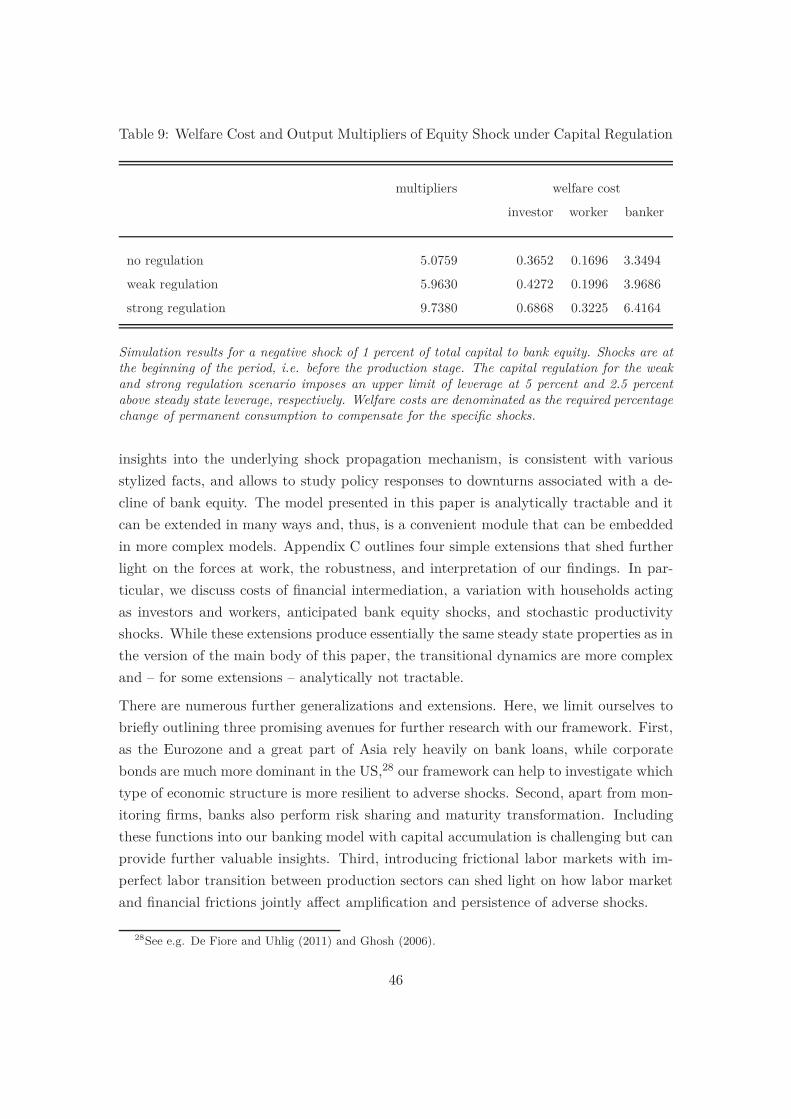
Table 9: Welfare Cost and Output Multipliers of Equity Shock under Capital Regulation
multipliers welfare cost
investor worker banker
no regulation 5.0759 0.3652 0.1696 3.3494
weak regulation 5.9630 0.4272 0.1996 3.9686
strong regulation 9.7380 0.6868 0.3225 6.4164
Simulation results for a negative shock of 1 percent of total capital to bank equity. Shocks are atthe beginning of the period, i.e. before the production stage. The capital regulation for the weakand strong regulation scenario imposes an upper limit of leverage at 5 percent and 2.5 percentabove steady state leverage, respectively. Welfare costs are denominated as the required percentagechange of permanent consumption to compensate for the specific shocks.
insights into the underlying shock propagation mechanism, is consistent with various
stylized facts, and allows to study policy responses to downturns associated with a de-
cline of bank equity. The model presented in this paper is analytically tractable and it
can be extended in many ways and, thus, is a convenient module that can be embedded
in more complex models. Appendix C outlines four simple extensions that shed further
light on the forces at work, the robustness, and interpretation of our findings. In par-
ticular, we discuss costs of financial intermediation, a variation with households acting
as investors and workers, anticipated bank equity shocks, and stochastic productivity
shocks. While these extensions produce essentially the same steady state properties as in
the version of the main body of this paper, the transitional dynamics are more complex
and – for some extensions – analytically not tractable.
There are numerous further generalizations and extensions. Here, we limit ourselves to
briefly outlining three promising avenues for further research with our framework. First,
as the Eurozone and a great part of Asia rely heavily on bank loans, while corporate
bonds are much more dominant in the US,28 our framework can help to investigate which
type of economic structure is more resilient to adverse shocks. Second, apart from mon-
itoring firms, banks also perform risk sharing and maturity transformation. Including
these functions into our banking model with capital accumulation is challenging but can
provide further valuable insights. Third, introducing frictional labor markets with im-
perfect labor transition between production sectors can shed light on how labor market
and financial frictions jointly affect amplification and persistence of adverse shocks.
28See e.g. De Fiore and Uhlig (2011) and Ghosh (2006).
46

References
Acemoglu, D. and Autor, D. (2011). Skills, tasks and technologies: Implications for
employment and earnings. In Ashenfelter, O. and Card, D., editors, Handbook of
Labor Economics, volume 4 of Handbook of Labor Economics, chapter 12, pages
1043–1171. Elsevier.
Acemoglu, D., Ozdaglar, A., and Tahbaz-Salehi, A. (2015). Systemic risk and stability
in financial networks. American Economic Review, 105(2):564–608.
Acharya, V. V., Gujral, I., Kulkarni, N., and Shin, H. S. (2011). Dividends and bank
capital in the financial crisis of 2007-2009. NBER Working Papers, Nr. 16896.
Acharya, V. V., Le, H., and Shin, H. S. (2017). Bank capital and dividend externalities.
Review of Financial Studies,, 30(3):988–1018.
Adrian, T. and Boyarchenko, N. (2012). Intermediary leverage cycles and financial
stability. Federal Reserve Bank of New York Staff Reports, 567.
Adrian, T. and Boyarchenko, N. (2013). Intermediary balance sheets. Staff Reports 651,
Federal Reserve Bank of New York.
Adrian, T. and Shin, H. S. (2014). Procyclical leverage and value-at-risk. Review of
Financial Studies, 27(2):373–403.
Allen, F. and Gale, D. (2009). Understanding Financial Crises. Clarendon Lectures in
Finance. Oxford University Press.
Alvarez, F. and Stokey, N. L. (1998). Dynamic Programming with Homogeneous Func-
tions. Journal of Economic Theory, 82(1):167–189.
Angeloni, I. and Faia, E. (2013). Capital regulation and monetary policy with fragile
banks. Journal of Monetary Economics, 60(3):3111–382.
Barany, Z. and Siegel, C. (2017). Job polarization and structural change. American
Economic Journal: Macroeconomics, (forthcoming).
Barlevy, G. (2004). The Cost of Business Cycles and the Benefits of Stabilization: A
Survey. NBER Working Papers 10926, National Bureau of Economic Research, Inc.
Bernanke, B. and Gertler, M. (1989). Agency costs, net worth, and business fluctuations.
American Economic Review, 79(1):14–31.
Bernanke, B., Gertler, M., and Gilchrist, S. (1996). The financial accelerator and the
flight to quality. Review of Economics and Statistics, 78(1):1–15.
47
Bloom, N., Floeotto, M., Jaimovich, N., Saporta-Eksten, I., and Terry, S. J. (2012).
Really uncertain business cycles. NBER Working Papers, Nr. 18245.
Bordo, M., Eichengreen, B., Klingebiel, D., and Martinez-Peria, M. S. (2001). Is the
crisis problem growing more severe? Economic Policy, 16(32):51–82.
Brumm, J., Grill, M., Kubler, F., and Schmedders, K. (2015). Collateral Requirements
And Asset Prices. International Economic Review, 56:1–25.
Brunnermeier, M. K. and Sannikov, Y. (2014). A macroeconomic model with a financial
sector. American Economic Review, 104(2):379–421.
Carlstrom, C. T. and Fuerst, T. S. (1997). Agency costs, net worth, and business
fluctuations: A computable general equilibrium analysis. American Economic Review,
87(5):893–910.
Challe, E. and Ragot, X. (2016). Precautionary saving over the business cycle. Economic
Journal, 126:135–164.
Christiano, L., Eichenbaum, M., and Evans, C. (2007). Shocks, structures or monetary
policies? the Euro area and US after 2001. Journal of Economic Dynamics and
Control, 32(8):2476–2506.
Contessi, S., Di Cecio, R., and Francis, J. (2013). Macroeconomic shocks and the two
sides of credit reallocation. Unpublished manuscript, Federal Reserve Bank of St.
Louis, MO.
Cooley, T., Marimon, R., and Quadrini, V. (2004). Aggregate Consequences of Limited
Contract Enforceability. Journal of Political Economy, 112(4):817–847.
De Fiore, F. and Uhlig, H. (2011). Bank finance versus bond finance. Journal of Money,
Credit, and Banking, 43(7):1395–1418.
De Fiore, F. and Uhlig, H. (2015). Corporate debt structure and the financial crisis.
Technical Report 8.
Diamond, D. W. and Rajan, R. G. (2000). A theory of bank capital. Journal of Finance,
55(6):2431–2465.
Ellingsen, T. and Kristiansen, E. G. (2011). Financial Contracting Under Imperfect
Enforcement. The Quarterly Journal of Economics, 126(1):323–371.
Fernald, J. G. (2015). Productivity and Potential Output before, during, and after the
Great Recession. NBER Macroeconomics Annual, 29(1):1–51.
48

Gersbach, H. and Rochet, J.-C. (2013). Capital regulation and credit fluctuations. CEPR
Discussion Papers, Nr. 9077.
Gersbach, H. and Rochet, J.-C. (2017). Capital regulation and credit fluctuations.
Journal of Monetary Economics, 90:113–124.
Gersbach, H., Rochet, J.-C., and Scheffel, M. (2016). Taking banks to solow. In Stiglitz,
J. E. and Guzman, M., editors, Contemporary Issues in Macroeconomics: Lessons
from The Crisis and Beyond, pages 176–198. Palgrave Macmillan UK, London.
Gertler, M. and Karadi, P. (2011). A model of unconventional monetary policy. Journal
of Monetary Economics, 58(1):17–34.
Gertler, M. and Kiyotaki, N. (2010). Financial intermediation and credit policy in
business cycle analysis. In Friedman, B. M. and Woodford, M., editors, Handbook of
Monetary Economics, volume 3, chapter 11, pages 547–599. Elsevier.
Ghosh, S. R. (2006). East Asian Finance: The Road to Robust Markets. World Bank,
Washington D.C.
Gomes, J., Jermann, U., and Schmid, L. (2016). Sticky leverage. mimeo, University of
Pennsylvania.
Hart, O. and Moore, J. (1994). A theory of debt based on the inalienability of human
capital. The Quarterly Journal of Economics, 109(4):841–79.
He, Z. and Krishnamurthy, A. (2013). Intermediary asset pricing. American Economic
Review, 103(2):732–770.
Holmstrom, B. and Tirole, J. (1997). Financial intermediation, loanable funds, and the
real sector. The Quarterly Journal of Economics, 112(3):663–91.
Itskhoki, O. and Moll, B. (2014). Optimal Development Policies with Financial Frictions.
NBER Working Papers, Nr. 19994.
Jermann, U. and Quadrini, V. (2012). Macroeconomic Effects of Financial Shocks.
American Economic Review, 102(1):238–271.
Kaplan, G., Violante, G. L., and Weidner, J. (2014). The wealthy hand-to-mouth. NBER
Working Papers, Nr. 20073.
Kiyotaki, N. and Moore, J. (1997). Credit cycles. Journal of Political Economy,
105(2):211–48.
49

Krebs, T. (2003a). Growth and Welfare Effects of Business Cycles in Economies with
Idiosyncratic Human Capital Risk. Review of Economic Dynamics, 6(4):846–868.
Krebs, T. (2003b). Human Capital Risk and Economic Growth. The Quarterly Journal
of Economics, 118(2):709–744.
Lucas, R. E. (1987). Models of Business Cycles. Yrjo Jahnsson Lectures. Basil Blackwell.
Martinez-Miera, D. and Suarez, J. (2012). A macroeconomic model of endogenous sys-
temic risk taking. CEPR Discussion Papers, Nr. 9134.
Meh, C. A. and Moran, K. (2010). The role of bank capital in the propagation of shocks.
Journal of Economic Dynamics and Control, 34(3):555–576.
Nuno, G. and Thomas, C. (2012). Bank leverage cycles. Banco de Espana Working
Papers, Nr. 1222.
Onali, E. (2014). Moral hazard, dividends, and risk in banks. Journal of Business
Finance and Accounting, 41(1,2):128–155.
Quadrini, V. (2011). Financial frictions in macroeconomic fluctuations. Economic
Quarterly, 97(3):209–54.
Quadrini, V. (2014). Bank liabilities channel. mimeo, University of Southern California.
Rampini, A. A. and Viswanathan, S. (2017). Financial intermediary capital. NBER
Working Papers, Nr. 23302.
Schularick, M. and Taylor, A. M. (2012). Credit booms gone bust: Monetary pol-
icy, leverage cycles, and financial crises, 1870-2008. American Economic Review,
102(2):1029–61.
Shin, H. S. (2016). Bank capital and monetary policy transmission. Technical report,
Bank for International Settlements.
Van den Heuvel, S. J. (2008). The welfare cost of bank capital requirements. Journal of
Monetary Economics, 55(2):298–320.
Zingales, L. (2011). The role of trust in the 2008 financial crisis. The Review of Austrian
Economics, 24(3):235–249.
50

A Appendix – Proofs
A.1 Appendix – Proof of Corollary 1
The partial derivatives of ϕ(λt) read
∂ϕ(λt)
∂λt= −
∂rMt (KM
t )
∂KMt
(λt − 1)Et −∂rI
t (KIt )
∂KIt
λtEt + rMt (KM
t ) − rIt (KI
t ) + θ > 0
∂ϕ(λt)
∂Ωt=
∂rMt (KM
t )
∂KMt
(λt − 1) < 0
∂ϕ(λt)
∂Et= −
∂rMt (KM
t )
∂KMt
(λt − 1)2 −∂rI
t (KIt )
∂KIt
λ2t > 0
∂ϕ(λt)
∂zM=
rMt (KM
t )
zM(λt − 1) > 0
∂ϕ(λt)
∂zI= −
rIt (KI
t )
zIλt < 0
∂ϕ(λt)
∂At=
(rMt (KM
t ) − rIt (KI
t ))λt − rMt (KM
t )
At< 0
∂ϕ(λt)
∂θ= λt > 0.
Because of inelastic labor supply and the Inada conditions, there will always be pro-
duction in both sectors, such that KIt > 0. Therefore, the leverage constraint implies
rMt (KM
t ) − rIt (KI
t ) + θ > 0. The inequalities follow from rMt (KM
t ) − rIt (KI
t ) + θ > 0,
λt > 1, and∂rj
t (Kjt )
∂Kjt
< 0. Total differentiation of ϕ(λt) and applying the implicit function
theorem yield ∂λt
∂At> 0, ∂λt
∂zI > 0, ∂λt
∂zM < 0, ∂λt
∂Ωt> 0, ∂λt
∂Et< 0, and ∂λt
∂θ < 0.
A.2 Appendix – Proof of Corollary 2
First, consider the impact on loan finance, KIt . When financial frictions are relevant, we
have KIt = λtEt. As of Corollary 1,
∂KIt
∂At= ∂λt
∂AtEt > 0 and
∂KIt
∂Ωt= ∂λt
∂ΩtEt > 0. Moreover,
using Equation (11) yields
∂KIt
∂Et=
∂λt
∂EtEt + λt
= −−
∂rMt (KM
t )
∂KMt
(λt − 1)2Et −∂rI
t (KIt )
∂KIt λ2
t Et
−∂rM
t (KMt )
∂KMt
(λt − 1)Et −∂rI
t (KIt )
∂KIt
λtEt + rMt (KM
t ) − rIt (KI
t ) + θ+ λt
=
−∂rMt (KM
t )
∂KMt
(λt − 1)Et + λt(rMt (KM
t ) − rIt (KI
t ) + θ)
−∂rM
t (KMt )
∂KMt
(λt − 1)Et −∂rI
t (KIt )
∂KIt
λtEt + rMt (KM
t ) − rIt (KI
t ) + θ> 0.
51

The inequality follows from rMt (KM
t ) − rIt (KI
t ) + θ > 0, λt > 1, and∂rj
t (Kjt )
∂Kjt
< 0.
Second, consider the impact on bond finance, KMt . When financial frictions are relevant,
KMt = Et + Ωt − λtEt. As of Corollary 1
∂KMt
∂At= − ∂λt
∂AtEt < 0. Moreover,
∂KMt
∂Ωt= 1 −
∂λt
∂ΩtEt
= 1 +
∂rMt (KM
t )
∂KMt
(λt − 1)Et
−∂rM
t (KMt )
∂KMt
(λt − 1)Et −∂rI
t (KIt )
∂KIt
λtEt + rMt (KM
t ) − rIt (KI
t ) + θ
=−
∂rIt (KI
t )
∂KIt
λtEt + rMt (KM
t ) − rIt (KI
t ) + θ
−∂rM
t (KMt )
∂KMt
(λt − 1)Et −∂rI
t (KIt )
∂KIt
λtEt + rMt (KM
t ) − rIt (KI
t ) + θ> 0
∂KMt
∂Et= 1 −
(
∂λt
∂EtEt + λt
)
= 1 +−
∂rMt (KM
t )
∂KMt
(λt − 1)2Et −∂rI
t (KIt )
∂KIt
λ2t Et
−∂rM
t (KMt )
∂KMt
(λt − 1)Et −∂rI
t (KIt )
∂KIt
λtEt + rMt (KM
t ) − rIt (KI
t ) + θ− λt
= −
∂rIt (KI
t )
∂KIt
λtEt + (λt − 1)(rMt (KM
t ) − rIt (KI
t ) + θ)
−∂rM
t (KMt )
∂KMt
(λt − 1)Et −∂rI
t
∂KIt
λtEt + rMt (KM
t ) − rIt (KI
t ) + θ
= −1 +
∂rIt (KI
t )
∂KIt
KIt + rI
t (KIt ) − θ
−∂rM
t (KMt )
∂KMt
(λt − 1)Et −∂rI
t (KIt )
∂KIt
λtEt + rMt (KM
t ) − rIt (KI
t ) + θ< 0,
where the third line uses the definition of leverage to rewrite (λt−1)(rMt (KM
t )−rIt (KI
t )+
θ) as 1 + rIt (KI
t ) − θ. The inequalities follow from rMt (KM
t ) − rIt (KI
t ) + θ > 0, λt > 1,∂rj
t (Kjt )
∂Kjt
< 0, and∂rI
t (KIt )
∂KIt
KIt + rI
t (KIt ) = αrI
t (KIt ) > 0.
The proof of point (iii) is obvious.
A.3 Appendix – Proof of Corollary 3
Note that Yt = Y Mt + Y I
t . Thus, ∂Yt
∂At=
∂Y Mt
∂At+
∂Y It
∂At> 0. When financial frictions are
binding,∂KM
t
∂Ωt= 1 −
∂KIt
∂Ωtand
∂KMt
∂Et= 1 −
∂KIt
∂Et. Thus, using Equation (11) yields
∂Yt
∂Ωt= rM
t (KMt )
∂KMt
∂Ωt+ rI
t (KIt )
∂KIt
∂Ωt= rM
t (KMt ) + (rI
t (KIt ) − rM
t (KMt ))
∂KIt
∂Ωt> 0
∂Yt
∂Et= rM
t (KMt )
∂KMt
∂Et+ rI
t (KIt )
∂KIt
∂Et= rM
t (KMt ) + (rI
t (KIt ) − rM
t (KMt ))
∂KIt
∂Et> 0.
52

The inequalities follow from∂KI
t
∂Ωt> 0,
∂KIt
∂Et> 0, and rI
t > rMt .
A.4 Appendix – Proof of Proposition 2
We consider a general structure that applies to both, the banks’ and the investors’
optimization problem. Consider the following optimization problem
maxCt,At+1
∞∑
t=0
βt ln Ct
subject to
(1 + τt)Ct + (1 + σt)At+1 = RtAt
where Ct is consumption, At is the agent’s net worth, τt is a consumption tax rate, σt is
an investment subsidy,29 and β is the discount factor. The problem captures of course
also the cases τt = 0 and σt = 0. The Euler equation reads
1 + σt
1 + τt
1
Ct= β
Rt+1
(1 + τt+1)Ct+1.
Suppose the consumption policy is Ct = c1+τt
RtAt where c is a constant. The Euler
equation in conjunction with the budget constraint can be rewritten as follows
1 + σt
1 + τt
1
Ct= β
Rt+1
(1 + τt+1)Ct+1
⇔1 + σt
cRtAt= β
Rt+1
cRt+1At+1
⇔1 + σt
cRtAt= β
1
cAt+1
⇔1 + σt
cRtAt= β
1 + σt
c(
RtAt − (1 + τt)Ct
)
⇔1
RtAt= β
1
RtAt − (1 + τt)Ct
⇔1
RtAt= β
1
RtAt − cRtAt
⇔1
RtAt= β
1
(1 − c)RtAt
⇔ c = 1 − β.
29An investment subsidy benefits investors for their total investment into both sectors by a factor1 + σt.
53

Thus, Ct = 1−β1+τt
RtAt. Moreover, the budget constraint yields
At+1 =1
1 + σt(RtAt − (1 + τt)Ct)
=1
1 + σt(RtAt − (1 − β)RtAt)
=1
1 + σtβRtAt.
A.5 Appendix – Proof of Proposition 7
We abstract from capital depreciation and any further taxes and subsidies. Consumption
of bankers in period t = 0 is constant if
(1 − d0)(RB0 E − ∆E + ∆T ) = (1 − βB)(RB
0 E − ∆E)
⇔ d0 = 1 − (1 − βB)RB
0 E − ∆E
RB0 E − ∆E + ∆T
. (A1)
where RB0 = 1 + rB
0 is the return on equity factor.
We next observe that
Ebb1 = d0(RB
0 E − ∆E + ∆T ) = βB(RB0 E − ∆E) + ∆T = Elf
1 + ∆T > Elf1 . (A2)
Ebb1 and Elf
1 denote the bank equity levels with balanced bailout and laissez-faire, re-
spectively. Property (A2) is a direct consequence of the scheme enacted in period 0. We
next observe that
Ebb1 + Ωbb
1 > Elf1 + Ωlf
1 . (A3)
The reason why inequality (A3) holds is that Ebb1 = Elf
1 +∆T while households suffering
a loss of ∆T will reduce savings by βH(∆T ) < ∆T .
As a consequence of Corollary 1, λbb1 < λlf
1 . However, we have
λbb1 Ebb
1 > λlf1 Elf
1 . (A4)
The latter property follows from the following contradiction. Suppose that λbb1 Ebb
1 =
KI,bb1 ≤ KI,lf
1 = λlf1 Elf
1 . Hence, KM,bb1 ≥ KM,lf
1 . As a consequence, rI,bb1 ≥ rI,lf
1 and
rM,bb1 ≤ rM,lf
1 . This leads to λbb1 ≥ λlf
1 which is a contradiction.
At the end of period 1 before consumption/savings decisions are made, the banker’s
wealth θλbb1 Ebb
1 with the balanced bailout is higher than under laissez-faire. Hence, the
54

policy-maker can again impose a dividend payout restriction 1−d1 < 1−βB that satisfies
(1 − d1)θλbb1 Ebb
1 = (1 − βB)θλlf1 Elf
1 .
We next show that rM,bb1 > rM,lf
1 for βH sufficiently high. Suppose to the contrary that
rM,bb1 ≤ rM,lf
1 , i.e.
KI,bb1 < KI,lf
1 + ∆T (1 − βH)
⇔1 + rM,bb
1
rM,bb1 − rI,bb
1 + θ(Elf + ∆T ) ≤
1 + rM,lf1
rM,lf1 − rI,lf
1 + θElf + ∆T (1 − βH).
Substituting rM,lf1 for rM,bb
1 further decreases the left-hand side of the inequality and
simplifying the condition then yields
Elf1 (−rI,lf
1 ) + ∆T (1 + rM,lf1 )(rM,lf
1 − rI,lf1 + θ) <
Elf1 (−rI,bb
1 ) + ∆T (1 − βH)(rM,lf1 − rI,bb
1 + θ).
For βH sufficiently close to 1, the relationship can only hold if KI,bb1 > KI,lf
1 +∆T (1−βH)
which is a contradiction. Hence, rM,bb1 > rM,lf
1 , λbb1 Ebb
1 > λlf1 Elf
1 , and Ebb1 + Ωbb
1 >
Elf1 + Ωlf
1 . We obtain
Ωbb1 (1 + rM,bb
1 ) + θλbb1 Ebb
1 = α
zM(
KM,bb1
LM
)α
+ zI(
KI,bb1
LI
)α
>
α
zM(
KM,lf1
LM
)α
+ zI(
KI,lf1
LI
)α
= Ωlf1 (1 + rM,lf
1 ) + θλlf1 Elf
1 , (A5)
as rI,bb1 > rM,bb
1 > rM,lf1 and KM,bb
1 + KI,bb1 > KM,lf
1 + KI,lf1 , more capital is invested in
the more productive sector.
At the end of period 1, households save βH(1 + rM,bb1 )Ωbb
1 and bankers are forced to save
according to the dividend payout restriction
d1θλbb1 Ebb
1 = θλbb1 Ebb
1 − θλlf1 Elf
1 + βBθλlf1 Elf
1 .
In combination with (A5), we get
βH(1 + rM,bb1 )Ωbb
1 + d1θλbb1 Ebb
1 > βH(1 + rM,lf1 )Ωlf
1 + βBθλlf1 Elf
1 .
Hence, after policy-makers impose a dividend payout restriction at the end of period 1
55

on bank equity – thereby keeping consumption of bankers unchanged – we obtain
Ebb2 > Elf
2 and Ebb2 + Ωbb
2 > Elf2 + Ωlf
2 .
A similar logic applies for the second and all subsequent periods.
B Appendix – Calibration
There are ten model parameters: the production parameters α, zM , and zM , the depre-
ciation rates δH and δB , the time preference factors βH and βB , the financial friction θ,
and labor endowment LM and LI . We calibrate the model to quarterly frequency using
quarterly and annual US data from 1998 to 2004 taken from the Federal Reserve Eco-
nomic Data (FRED), the Federal Deposit Insurance Corporation (FDIC) Call Report
Data, and the Penn World Table (PWT) and proceed as follows. As only the relative
productivity affects the steady state allocation, we normalize zM = 1 without loss of
generality. In a similar vein, we normalize LM = 1. The output elasticity of capital is
set to α = 0.36, which is in the range of values suggested in the literature.
We equalize depreciation rates on household wealth and bank equity, i.e. δB = δH = δ.
Let s denote the aggregate saving rate. The capital-to-output ratio simplifies to K/Y =
s/δ. Choosing the saving rate to match the gross-saving-to-GNP ratio taken from the
FRED NIPA accounts, i.e. s = 0.1872, and setting the capital-to-output ratio equal to
the respective series from the Penn World Table, i.e. K/Y = 12 on a quarterly base,
delivers δ = 0.0156.
According to FRED, we set the average annual return on bank equity to 14.26 percent
which produces a quarterly return (1 + rB)4 = 1.1426, i.e. rB = 0.0339. Moreover,
taking the calibration target for bank leverage from the aggregated Call Report Data
provided by the FDIC, λ = 10.7449, the definition for return on equity rB = θλ − δ − 1
yields θ = 0.0977 and the steady state condition for bank equity yields βB = 1/(θλ−δ) =
0.9672.
According to De Fiore and Uhlig (2011), the average bond-to-loan finance ratio in the
US is KM/KI = 1.5000. In order to attribute return differences solely to relative
differences in productivity z, capital-to-labor ratios in sector M and I have to be equal.
Thus, we set LI = 2/3 as LMt has been normalized to 1. Furthermore, combining the
target for the bond-to-loan finance ratio with the aggregate resource constraint gives
KI = K/(1 + KM /KI). The steady state condition for investor wealth and the leverage
56

condition with A = 1 read
KM
LM=
(
αzM
1βH
+ δ − 1
)1/(1−α)
KI
LI=
(
αλzI
(λ − 1)( 1
βH+ δ − 1
)
+ θλ − 1
)1/(1−α)
.
Using KM = KM/KIKI , we combine both conditions to substitute for KI and obtain
zI(LI)1−α =(λ − 1)
(
1βH
+ δ − 1)
+ θλ − 11
βH+ δ − 1
zM
λ
(
LM
KM /KI
)1−α
. (B1)
Moreover, the capital-to-output ratio is
K/Y =(1 + KM /KI)KI
zI(KI)α(LI)1−α + zM (KM /KI)α(KI)α(LM )1−α
=1 + KM /KI
zI(LI)1−α + zM (KM /KI)α(LM )1−α(KM /KI)α−1 αzM
1βH
+ δ − 1(LM )1−α, (B2)
where the second line uses the steady state condition for investor wealth and the bond-
to-loan finance ratio to substitute for KI . Using (B1) in (B2) and solving for βH , we
obtain
βH =
(
1 − δ +αλ1+KM /KI
K/Y− (θλ − 1)
λ(1 + KM/KI) − 1
)−1
= 0.9865
which is within the range of values used for annual calibration in the literature. Finally,
Equation (B1) yields zI = 1.0644. The calibrated parameter values and the calibration
targets are summarized in Table 2.
C Appendix – Extensions
In this Appendix, we discuss four extensions that help to understand the main channel
through which shocks get propagated, the robustness of the findings, and the interpre-
tation of the model.
C.1 Cost of Intermediation
So far, we have assumed that banks do not incur real cost when they monitor en-
trepreneurs. Typically, however, commercial or universal banks have to spend consid-
57

erable resources on such activities. Such cost can easily be integrated in our model.
Suppose, e.g., that banks incur a cost c (c > 0) per unit of loans they monitor. Then,
the non-pledgeable part increases to (c+θ)KIt , while bankers only obtain θKI
t from their
lending activities. The market-imposed leverage constraint, Equation (5), adjusts to
KIt =
1 + rMt
rMt − rI
t + θ + cEt.
The solution of the model follows similar lines as for the baseline model Specifically,
similar to Section 5, we get
rM = δ + ρH
θλ = δ + ρB + 1
λ =1 + δ + ρH
δ + ρH − rI + θ + c=
1 + δ + ρB
θ
rI = rM +θ(ρB − ρH)
1 + δ + ρB+ c.
Hence, steady state leverage λ and the return on equity θλ are unaffected by cost of
intermediation. However, less capital can be invested in sector I which reduces both the
level of bank equity and investor wealth in the steady state.
C.2 Workers also Save
We consider a variant of the model in which households are not divided into investors
and workers, such that there are only two types of agents: households and bankers.
The former own the capital stock Ω and supply labor inelastically. The problem of
the household is the same as the one described in Section 3.2, except for the budget
constraint (3), which now includes labor income
CHt + Ωt+1 = wI
t LI + wMt LM + Ωt(r
Mt + 1 − δ).
Optimization yields the standard Euler equation for the household problem
1
CHt
= βH(1 + rMt+1 − δ)
1
CHt+1
. (C1)
The steady state condition derived from the households’ necessary condition remains un-
affected. As there is no change in the banker’s first-order-condition either, the following
proposition ensues:
58
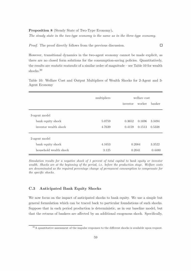
Proposition 8 (Steady State of Two-Type Economy).
The steady state in the two-type economy is the same as in the three-type economy.
Proof. The proof directly follows from the previous discussion.
However, transitional dynamics in the two-agent economy cannot be made explicit, as
there are no closed form solutions for the consumption-saving policies. Quantitatively,
the results are mutatis mutandis of a similar order of magnitude – see Table 10 for wealth
shocks.30
Table 10: Welfare Cost and Output Multipliers of Wealth Shocks for 2-Agent and 3-Agent Economy
multipliers welfare cost
investor worker banker
3-agent model
bank equity shock 5.0759 0.3652 0.1696 3.3494
investor wealth shock 4.7639 0.4159 0.1513 0.5338
2-agent model
bank equity shock 4.1653 0.2084 3.3522
household wealth shock 3.125 0.2041 0.4480
Simulation results for a negative shock of 1 percent of total capital to bank equity or investorwealth. Shocks are at the beginning of the period, i.e. before the production stage. Welfare costsare denominated as the required percentage change of permanent consumption to compensate forthe specific shocks.
C.3 Anticipated Bank Equity Shocks
We now focus on the impact of anticipated shocks to bank equity. We use a simple but
general formulation which can be traced back to particular foundations of such shocks.
Suppose that in each period production is deterministic, as in our baseline model, but
that the returns of bankers are affected by an additional exogenous shock. Specifically,
30A quantitative assessment of the impulse responses to the different shocks is available upon request.
59

let
rBt =
θλ(rMt , rI
t ) − δ − 1 with probability 1 − ν
κ(θλ(rMt , rI
t ) − δ) − 1 with probability ν,
where 0 < κ < 1 and 0 < ν < 1. The shocks to bank equity are independently and iden-
tically distributed across time and realized before the bankers make their consumption-
saving decision. Typically for the context of banking crises, ν is assumed to be rather
small and thus such shocks occur infrequently. The bankers’ Euler equation reads
1
CBt
= βBEt
[
1 + rBt+1
CBt+1
]
,
where Et denotes the expectation formed at the end of period t. As current shocks
are realized when the consumption-saving decision is made, the functional form of the
saving policy remains unaffected compared to the non-stochastic case. Specifically, CBt =
(1 − βB)(1 + rBt )Et and Et+1 = βB(1 + rB
t )Et, i.e. saving rates remain constant with
respect to end-of-period equity. Hence, with high probability, the dynamics associated
with anticipated negative shocks to bank equity are approximately the same as if such
shocks occurred unanticipated at the deterministic steady state provided that the shocks
are sufficiently rare. The reason is that with very high probability, the economy is close
to its steady state when a negative bank equity shock occurs.31
C.4 Stochastic Productivity Shocks
In analogy to the real business cycle literature, we introduce stochastic productivity.
Typically, we assume
At = Aeat , at = ρat−1 + ηt,
where ηt is an independent and identically, normally distributed random variable with
mean zero and variance σ2η . The parameter ρ (0 < ρ < 1) measures the persistence of the
shock that follows an autoregressive model of order one. By using the same argument
as in the previous section, we see that the saving rates with respect to end-of-period
wealth of bankers and investors remain unaffected by uncertainty about future returns
to capital and bank equity. Hence, the laws of motion essentially remain the same, but
with stochastic time paths of all economic variables.
31Assuming larger probabilities for negative bank equity shocks would allow to investigate limit distri-butions and stochastic steady states. For instance, leverage is distributed symmetrically in our calibrationif we set κ = 0.8 and ν = 0.2.
60

D Appendix – List of Notations
parameter/variable description
i = H, W, B index for investor (H), worker(W ), and banker(B)
j = M, I index for production sector bond financed (M) and loan financed (I)
Et bank equity
Ωt household wealth
Γ partition on state space for which financial frictions are binding
Cit consumption of agent i = H, W, B
Kjt capital input in sector j = M, I
Kt total capital endowment
Dt investment in deposits
Bt investment in bonds
Lj labor input in sector j = M, I
L total labor endowment
lj share of labor endowment devoted to sector j = M, I
ℓ relative labor input ℓ.= LI/LM
rjt capital return in sector j = M, I
rDt deposit rate
wjt wage rate in sector j = M, I
λt bank leverage
At common productivity
zjt sector specific productivity in sector j = M, I
z relative productivity z.= (zI/zM)1/(1−α)
α output elasticity
δ capital depreciation rate
θ financial friction
βi discount factor of agent i = H, W, B
ρi discount rate of agent i = H, W, B
61


