

Flexible Automatic Generation Control System for
Embedded HVDC Links
Francisco Gonzalez-Longatt
Loughborough University
School of Electric, Electronic and
Systems Engineering
Loughborough, United Kingdom
Anton Steliuk
DMCC Engineering Ltd
Peremogy ave., 56, Kyiv, 03056
Ukraine
Víctor Hugo Hinojosa M Universidad Técnica Federico Santa
María, Department of Electrical
Engineering Valparaiso-Chile
Abstract— Future power systems are expected being operated
under increasingly stressed conditions and increased
uncertainties. The future single European electricity market will
entail higher energy trading volumes, for which augmented use
of HVDCs is expected to facilitate cross-border bulk power
transfers. In traditional power systems a change in demand at
one point of network is reflected throughout the system by a
change in frequency. However, significant interconnections
using HVDC will affect the classical ability of traditional AC
system to overcome “together” frequency deviations which may
result in a cascading failure and system collapse. Future HVDC
systems shall fulfil requirements referring to frequency stability
and also intervening in the frequency quality. As consequence
HVDC systems will operate providing ancillary service depends
on the framework of service. This paper proposes a flexible
Automatic Generation Control (AGC) system for embedded
HVDC links in order to provide frequency sensitive response
and control power interchange.
Index Terms-- Automatic generation control, frequency
controller, frequency stability, power system, protection scheme,
wind turbine generator.
I. INTRODUCTION
Future energy systems networks will be completely
different to the power systems on nowadays [1], [2]. High
and low power converters will be massively deployed in
several areas on the electric network [3], [4]: (i) renewable
energy from highly variable generators connected over high
power converters, (ii) several technologies for energy storage
with very different time constants, some of them using power
converters as an interface to the grid, and (iii) Pan-European
transmission network facilitating the massive integration of
large-scale renewable energy sources and transportation of
electricity based on underwater multi-terminal high voltage
direct current transmission. The developments of stronger
interconnector and massive integration of offshore wind
power in remote location are steadily increasing the demand
for more robust, efficient, and reliable grid integration
solutions. Multi-terminal Voltage source converter (VSC)-
based HVDC (MTDC) technology has the potential to
increase transmission capacity, system reliability, and
electricity market opportunities.
The integration of VSC-HVDC links into transmission
systems has the potential to afford a powerful new tool for
controlling both over and under frequency conditions. The
high degree of controllability inherent to the active power
flow on HVDC links allow rapid changes of power flows to
be used to counter active power imbalances [5].
Primary frequency control in HVDC has been a hot topic
in recent times. Several publications have developed and
tested controllers to enable inertial response on HVDC
systems [6-9]. HVDC for primary frequency control has been
considered in several publications [10], [11], and the
coordinated primary frequency control among non-
synchronous systems connected by a multi-terminal HVDC
grid has been studied in [12]. In addition, the problem of
providing frequency control services, including inertia
emulation and primary frequency control, from offshore wind
farms connected through a MTDC network has been studied
in [13]. However, secondary and tertiary frequency control
considering HVDC or MTDC systems has deserved a very
low attention in recent publications.
This paper proposes a flexible Automatic Generation
Control (AGC) system for embedded HVDC link in order to
provide frequency sensitive response and control power
interchange. The paper is organized as follows: Section II
briefly defines the main considerations about DC-
Independent System Operator (DC-ISO) and Section III
establishes the short backgrounds about DC-voltage control
in MTDC systems. Section IV focuses the proposed optimal
power flow in system based on DC-ISO objectives. Section V
illustrates application examples on a representative test
system of a future DC-ISO. Finally, section VI results are
tabulated for assessment and comparisons.

II. FREQUENCY CONTROL
Frequency control in power systems is usually formed of
primary and secondary control. Future power system will
require an active participation of HVDC to support the
primary and secondary frequency control.
Frequency control can be considered to be one of the most
crucial aspects of ancillary services. It is responsible that the
power system operates within acceptable frequency limits.
The classical approach of frequency control can
schematically be divided by three stages: primary, secondary
and tertiary control. This is a tiered approach where
controllers are responsible of frequency containment,
frequency restoration and replacement reserves, respectively.
The primary control refers to control actions that are done
locally (on the power plant level) based on the set-points for
frequency and power. The objective of the primary control is
to maintain the balance between generation and load [1] as
consequence stabilizes the frequency after a disturbance. The
primary frequency controllers are typically a simple
proportional controller. A generating unit participating in
primary control uses a proportional constant in the controller,
named speed droop D. The constant provides the relationship
between momentary frequency deviation (f) and change in
electric power production (P), D = f /P in Hz/MW
Post-disturbance steady-state frequency differs from the
nominal frequency, especially because the droop
characteristics in primary controllers and the load self-
regulation effect. The secondary frequency control, also
called Load Frequency Control (LFC), adjusts power set-
points of the generators in order to compensate for the
remaining frequency error after the primary control has acted.
The purpose of secondary control actions is to restore the
system frequency to the nominal set point, and ensure that
any tie-line flows in the system are at their contracted level.
LFC can also be performed manually as in case of the Nordel
powers system and [14], Continental Europe interconnected
system (ENTSO-e) and National Grid Transco (NGT) in
England and Wales [15], uses an automatic scheme which
can also be called Automatic Generation Control (AGC).
Global analysis of the power system markets shows that the
AGC is one of the most profitable ancillary services at these
systems [16].
The AGC is a controller created for the following
functions [17]: (i) maintain frequency at the scheduled value
(frequency control); (ii) maintain the net power interchanges
with neighboring control areas at their scheduled values (tie-
line control); and (iii) maintain power allocation among the
units in accordance with area dispatching needs (energy
market, security or emergency).
In some interconnected power systems, the role of AGC
may be restricted one or two of the above objectives. For
instance, tie-line power control is only used where a number
of separate power systems are interconnected and operate
under mutually beneficial contractual agreements.
Based on the above objectives, two variables frequency
and tie line power exchanges are weighted together and used
into the supplementary feedback loop. A suitable linear
combination of frequency (fi = fi -fset) and tie-line power
changes (Ptie,i= Ptie,i - Ptie,iset) for area i, is known as the Area
Control Error (ACE):
, ,i tie i bias i iACE P f (1)
where βbias,i is a bias factor. ACE corresponds to the power by
which the total area power generation must be changed in
order to maintain both frequency and tie-line flows at their
scheduled values. The AGC is a central frequency regulator
which uses an integrating element in order to remove any
error and this may be supplemented by a proportional
element. For such a PI regulator the output signal is:
, , ,AGC i P i i I i iP K ACE K ACE dt (2)
The aim of the frequency bias factor βbias,i is to fully
compensate for the initial frequency response of the area. It
can be demonstrated that independent of the choice of βbias,i
the frequency deviation will eventually be returned to zero so
that the choice of βbias,i is not critical for the system. The
regulator in an area tries to restore the frequency and net tie-
line interchanges after an imbalance, so it enforces an
increase in generation equal to the power deficit. The
regulation is executed by changing the power output of power
plants in the area through varying Pref,i in their governing
systems.
The regulator output signal Pref is then multiplied by the
participation factors α1, α2, …, αn which define the
contribution of the individual generating units to the total
generation control as shown on Fig 1.
ACE
Pf
+
-
Ptie
Ptie,ref
λR
+
fmeas
fref
-
-
-PI
α1
α2
αi
αn
Pref1
Pref2
Prefi
Prefn
Pref
Figure 1. Functional diagram of a central regulator [17].
The control signals Pref1, Pref2, …, Prefn obtained in this
way are then transmitted to the power plants and delivered to
the reference set points of the turbine governing systems.
During the last decades, there has been a large amount of
research into alternatives to the classical AGC control
formulation. With the advent of advanced control theory
many new solutions have been proposed. A summary of the
research into such topics is provided in [18], [19].
III. AUTOMATIC GENERATION CONTROL (AGC)
The structure of the AGC of the interconnected power
system (IPS) is shown in Fig. 2. It consists of n power plants

with generation units participating in frequency support.
Control levels
System
Levelfsys
fref Pnet,ref
Pflow,k
Power
controller 1
Governor 1,1
AGC of the Area
...
Power
plant 1 fP1
Governor 1m
P1mP11
Pt1mPt11
PAGC,1
Power
Plant
Level
Generation
Unit
Unit Level
Power
controller n
Governor nm
Power
plant n
Governor n1
Pn1 Pmn
Ptn1
Gnm
... ...
PAGC,n
Pflow,1
Pflow,m
f1,1
G11 G1m
...
...
f1,m fn,1
Gn1
Ptnmfn,m
...
...
...
fPn
...
...
Figure 2. The structure of the Interconnected Power system and
representation of the AGC.
There are three control levels of the active power and
frequency control. The upper system control level is
presented by the AGC of the area (system level). The input
signals are the system frequency measurement fmeas=fsys in the
power system, and the scheduled power on the interface (Ptie
line interchanges Pflow,k.
Based on tie-line interchanges Pflow,k, the net interchange
power (Pnet,ref) is calculated by:
, ,
1
branchesN
net ref flow k
k
P P
(3)
In the AGC of the IPS, the system frequency deviation
(f) and the changes on the net interchange power (Pnet)
deviations are defined as:
sys reff f f (4)
,net net net refP P P (5)
where: fref is a frequency set point value (typically, the rated
or nominal frequency), Pnet.ref is a net interchange power set
point value.
The area control error (ACE) is calculated in similar way to
(1) as:
net biasACE P K f (6)
where: Kbias is the frequency bias.
In the event of internal power imbalance of the IPS, ACE
defines the power to be compensated by the regulating power
plants in this IPS [20]. In case of external frequency
disturbance, due to different signs of frequency and net
interchange power deviations, ACE value tends to zero. The
AGC operation depends on location of the disturbance [20],
[21].
The unscheduled active power setting PAGC formed by the
proportional-integral (PI) controller is calculated as follows: 2
1
t
AGC P I
t
P K ACE K ACEdt (7)
where: KP is the proportional gain of the PI controller; KI is
the integral gain of the PI controller; t1, t2 are the integration
limits. As shown in Fig. 2, the i-AGC control signal PAGCi, is
transmitted to each regulating power plant according to the
participation factor αi of each individual power plant in the
secondary frequency control:
, αAGC i i AGCP P i = 1, 2, …, n (8)
At the power plant control level the signal PPCi formed by
the power plant PI controller is calculated as: 2
11 1
tm mPC PC
PCi P f agci Tj I f agci Tj
j jt
P K K f P P K K f P P dt
(9)
where: KPPC is the proportional gain of the power plant PI
controller; KIPC is the integral gain of the power plant PI
controller; Kf is the coefficient of frequency correction; PT
is the sum of the turbine power change of the generating units
participating in the secondary frequency control, and i = 1, 2,
…, n,.
The distribution of the control signal PPCi at the i-power
plant control level is performed in accordance with the
participation factors βij of the generating units in the
secondary frequency control (see Fig. 2):
βij ij PCiP P i = 1, 2, …, n and j = 1, 2,…,m (10)
where: n is the number of regulating power plants; m is the
number of generating units of the i-power plant; ∆Pij is the
control signal from the power plant controller. The control
signal ΔPij.ref is distributed in such a way that:
1
m
PCi ij
j
P P
i = 1, 2, …, n (11)
and
1 1 1
n n m
agc agci ij
i i j
P P P
(12)
The calculated control signal ΔPij from the power
controller is transmitted to the turbine governor of the
generating unit (aggregate control level) using the speed
changer motor (see Fig. 2). Further, according to the
reference control signal ΔPij, the turbine governor generates a
signal for the turbine power change ΔPtij. Thus, the power
changing of the generating units restores the normal
frequency and scheduled net interchange power.
IV. PROPOSED AGC INCLUDING EMBEDDED HVDC LINK
Future power system will require an active participation of
HVDC grids to support the AGC function of frequency
control. The classical approach presented on Section III is
expanded to a hybrid AC/DC system where a HVDC link is
embedded in a traditional AC system. The structure of the
proposed controller enabling the participation of HVDC link
on the AGC support is presented in Fig. 3. There are four
control levels of the active power and frequency control. The
upper system control level is presented by the AGC of the
power system. The input signals are the system frequency
measurement fmeas in the power, the scheduled power on the
interface (Ptie ) and line interchanges (AC lines: Pflow,k, and
DC lines: PDC,ij).

Control levels
System
Levelfsys
fref Pnet,ref
Pflow,k
Power
controller 1
Governor 1,1
AGC of the Area
...
Power
plant 1 fP1
Governor 1m
P1mP11
Pt1mPt11
PAGC,1
Power
Plant
Level
Generation
Unit
Unit Level
Power
controller n
Governor nm
Power
plant n
Governor n1
Pn1 Pmn
Ptn1
Gnm
... ...
PAGC,n
Pflow,1
Pflow,m
f1,1
G11 G1m
...
...
f1,m fn,1
Gn1
Ptnmfn,m
...
...
...
fPn
...
...
PDC,ref
PDC,ij
PDC,ij
HVDC
Link
Level
PDC,ij
...
Figure 3. The structure of the hybrid AC/DC Interconnected Power system
and considering the proposed AGC controller.
Based on tie-line interchanges, the net interchange power
(Pnet,ref) is calculated as:
, , ,
1
branchesN
net ref flow k DC ij
k
P P P
(13)
In the AGC of the power system, the system frequency
deviation (f) and changes on the net interchange power
(Pnet) deviations are calculated using (4) and (5). Also the
ACE is calculated using (6). In this paper, the proposed AGC
includes a control system to provide signals to embedded
HVDC links in order to provide frequency sensitive response
and control power interchange. The control is designed to
make use of the fast response and lower loses of the HVDC
system and alleviate the AC transmission system in the
interface between the ISPs. A proportional controller is used
to define the change on the HVDC based on the AGC: 0
, ,DC ref DC ref HVDCP P ACE (14)
subject to: min max
,DC DC ref DCP P P (15)
where 0
,DC refP is pre-contingency power flow on the HVDC
link and max
DCP , min
DCP power limit of the converter station.
V. SIMULATION AND RESULTS
In this Section, a hybrid AC/DC test network is used to
illustrate and test the proposed controller. The classical IEEE
14-bus test system is used as AC test network. It represents a
portion of the American Electric Power System (in the
Midwestern USA) in February, 1962. The original IEEE 14-
bus system (as presented on [22], [23]) has been slightly
modified, so the system has three Power Plants and a
boundary has been defined to establish 2 operational areas
(Area 1 and Area 2 in Fig. 4). Not depicted in Fig. 4, but
included in the system model, are generator controllers (IEEE
Type 1 speed-governing model and the automatic voltage
regulators - SEXS, Simplified Excitation System).
Net interchange power
Area 1
Area 2
Power
Plant 3
Power
plant 2
Power
plant 1
IEEE 14 bus Test model
G3
1 B
us
G21 Bus
G3
_2
Bu
s
G1 Bus
G22 Bus
Bus 8
Bus 6
Bus 11 Bus 10
Bus 9
Bus 14Bus 13
Bus 12
Bus 3
Bus 2
Bus 1
Bus 5Bus 4
fglongatt.org
PowerFactory 15.1.6
IEEE 14 Bus Test system - AGC simulation
Prof. FGL, Dr A. Steliuk, Dr V Hinojosa Automatic Generation Control: Simulation
Frequency Stability
Project: Graphic: Test network Date: 11/14/2014 Annex: 1
Load 1
Add load
Tr-G3-1Tr-G3-1
G~
G3
1
Tr-
G2
-1T
r-G
2-1
G~G21
Tr-G32Tr-G32
Tr-
G1
Tr-
G1
Tr-
G2
-2T
r-G
2-2
4-7
7-8
7-9
4-7
7-8
7-9
4-7
7-8
7-9G~
SC
6
G ~G
33
G ~
CS
8
5-6
5-6
4-9
4-9
G~ G22
G~
G1
Load 2
Load 3 Lo
ad
4
Lo
ad
5
OHL 1-5OHL 1-5
OHL 1-2 /2OHL 1-2 /2
OHL 1-2 /1OHL 1-2 /1
OHL 2-5OHL 2-5 OHL 4-5OHL 4-5
OHL 2-4OHL 2-4
OHL 2-3OHL 2-3
OH
L 3
-4O
HL
3-4
Lo
ad
6
Load 9
Load 10Load 11
Load 12
Load 14Load 13
6-1
16
-11 OHL 10-11OHL 10-11
9-1
09
-10
9-1
49
-14
OHL 13-14OHL 13-14
OH
L 6
-13
OH
L 6
-13
OHL 6-12OHL 6-12
OHL 12-13
OHL 12-13
DIg
SIL
EN
T
Figure 4: Test System: Modified IEEE 14-bus test system.
The interface between Area 1 and Area 2 is defined by
three overhead transmission line OHL 1-5, OHL 1-2/1 and
OHL 1-2/2, as consequence the AGC is developed to monitor
and control the net power interchange on them.
DIgSILENT® PowerFactoryTM is used for time-domain
(RMS) simulations and DIgSILENT Simulation Language
(DSL) is used for dynamic modelling of all controllers.
All simulations are performed using a PC based on Intel®,
CoreTM i7-7410HQ CPU 2.5GHz, 16 GB RAM with
Windows 8.1 64-bit operating system.
The proposed AGC model enabling the participation of the
HVDC link in the AGC support has been developed using
DSL. Figure 5 shows the DSL implementation of the generic
AGC controller. Active power flow measurements on OHL 1-
5 (Pflow1), OHL 1-2/1 (Pflow2), and OHL 1-2/2 (Pflow3) are used
for monitoring the net power interchange. In addition, a
measurement device (ElmPphi) is used to obtain the system
frequency (fsys). AGC AREA-2 frame:
AGC slot
Power flow and
frequency
measurement slots
AGC ControllerElmAgc*
0
1
2
3
0
1
Frequency meaElmPhi*
Power flow Pflow3StaPqmea*
Power flow Pflow2StaPqmea*
Power flow Pflow1StaPqmea*
AGC AREA-2 frame:
fmeas
Pflow3
Pflow2
Pflow1
DIg
SIL
EN
T
Figure 5. General frame of the AGC model.
Fig. 6 shows the DSL model created for the proposed
controller, including the classical AGC and enhancing the
participation of the HVDC link in frequency control. Five
subsystems have been highlighted on the general frame:
Frequency deviation calculation, Calculation of net
interchange power deviation, PI controller, signals calculation
of the AGC and HVDC contribution.
Three scenarios have been simulated in order to evaluate
the performance of the controllers and to demonstrate the
suitable operation of the proposed controllers:

Case I, No AGC: This simulation scenario is based on the
AC network (IEEE 14-bus) and considering the inertial
and governor response. AGC is not active in this case.
The idea of this base case is to demonstrate that a system
frequency disturbance creates power imbalance which is
covered by the governors, however, the final operational
frequency is reduced by the action of the droop.
Case II: Classic AGC: A classic AGC controller is
enabled in this simulation scenario allowing the
frequency recovery after the system frequency
disturbance.
Case III: Proposed AGC: under this scenario the HVAC
overhead transmission line OHL1-5 is substituted by a
HVDC link. Now, the proposed AGC is enabled in the
hybrid AC/DC network in order to test the proposed
controller.
AGC AREA2 controller:
HVDC Contribution
Calculation ofthe net interchange power
deviation
Frequency deviationcalculation
AGC control signals calculation
PIcontroller
ConstGammaHVDC
ConstGamma32
ConstGamma31
ConstGamma22
ConstPnetr..
ConstKbias
-
ConstGamma21
[Kp+Ki/s]Kp,Ki
Pagc_max
Pagc_min
Constfref
-
1/basePbase
-
AGC AREA2 controller:
0
2
3
1
1
2
3
4
0dPdc
o5
fmeas
o4
o3
o1
dP
net
yi
o2
Pnet
dP32
dP31
dP22
dP21PagcBia
s_fa
ct
df
fr
o19
ACEKbiasdf
Pflow1
Pflow3
Pflow2
DIg
SIL
EN
T
Figure 6. General frame of the Proposed AGC control model.
TABLE I. SUMMARY OF SIMULATION RESULTS
Case I II III
Initial state Post-contingency Steady State
Output Power at Generators (MW)
Gen 1 225 (221.3) 232.4 225.3 221.2
Gen 21 150 (148.9) 157.0 160 159.3
Gen 22 150 (148.9) 157.0 160 159.3
Gen 31 150 (148.9) 157.0 159 159.4
Gen 32 150 (148.9) 157.0 159 159.4
Power flows (MW)
OHL 1-2/1 -17 (-16.2) -16.4 -13.5 -9.5
OHL 1-2/2 -16.9 (-16.1) -16.3 -13.5 -9.4
OHL 1-5 -56.3 -64.9 -63.5 --
HVDC --56.6 -70.2
Net flow -90.2 (-88.6) -97.7 -90.6 -89.1
Number between parentheses shows the initial condition of Case III. The use
of HVDC link reduces power losses as consequence power generations and
power flows are different.
A simple contingency is simulated, it is an events based on
step increase on the power demand at load 6 (PL6 = 44.8
MW). Plots of main electromechanical associated to the
system frequency response are shown on Fig. 6 and 7. Case II
is used to illustrate how the steady-state post contingency
frequency is recovered after the system frequency event,
without AGC (Case I) a decreased frequency, 49.94 Hz is
observed. Also, the positive effect of the classical AGC (Case
II) on reestablishing the net interchange power flow at the
interface is shown on Fig. 7. A summary of the pre and post
contingency steady-state, power generation and power flows,
for several cases is shown on Table I. Results on Table I
demonstrate the capacity of the proposed controller (Case III)
to modify the power flow on the interface increasing the
power transfer on the HVDC link, decreasing the power on
OHL 1-1/2 and OHL 1-2/2 ( around -44%), also the correct
performance is shown on the faster recovery on the frequency
compare to Case II.
100,080,060,040,020,00,0 [s]
161,50
159,00
156,50
154,00
151,50
149,00
Generator 31: Pgen in MW Case I
Generator 32: Pgen in MW Case I
Generator 31: Pgen in MW Case II
Generator 32: Pgen in MW Case II
150 MW
157 MW 159 MW
100,080,060,040,020,00,0 [s]
236,50
234,00
231,50
229,00
226,50
224,00
Generator 1: Pgen in MW Case I
Generator 1: Pgen in MW Case II
225 MW
232.4 MW
225.3 MW
100,080,060,040,020,00,0 [s]
161,50
159,00
156,50
154,00
151,50
149,00
Generator 21: Pgen in MW Case I
Generator 22: Pgen in MW Case I
Generator 21: Pgen in MW Case II
Generator 22: Pgen in MW Case II
150 MW
157 MW 160 MW
100,080,060,040,020,00,0 [s]
50,03
50,00
49,97
49,94
49,91
49,88
Bus 2: Freq in Hz Case I
Bus 2: Freq in Hz Case II
49.94 Hz
DIg
SIL
EN
T
100,080,060,040,020,00,0 [s]
161,50
159,00
156,50
154,00
151,50
149,00
Generator 31: Pgen in MW Case I
Generator 32: Pgen in MW Case I
Generator 31: Pgen in MW Case II
Generator 32: Pgen in MW Case II
150 MW
157 MW 159 MW
100,080,060,040,020,00,0 [s]
236,50
234,00
231,50
229,00
226,50
224,00
Generator 1: Pgen in MW Case I
Generator 1: Pgen in MW Case II
225 MW
232.4 MW
225.3 MW
100,080,060,040,020,00,0 [s]
161,50
159,00
156,50
154,00
151,50
149,00
Generator 21: Pgen in MW Case I
Generator 22: Pgen in MW Case I
Generator 21: Pgen in MW Case II
Generator 22: Pgen in MW Case II
150 MW
157 MW 160 MW
100,080,060,040,020,00,0 [s]
50,03
50,00
49,97
49,94
49,91
49,88
Bus 2: Freq in Hz Case I
Bus 2: Freq in Hz Case II
49.94 Hz
DIg
SIL
EN
T
100,080,060,040,020,00,0 [s]
-55,50
-58,00
-60,50
-63,00
-65,50
-68,00
OHL 1-5: Pflow in MW Case I
OHL 1-5: Pflow in MW Case II
-56.3 MW
-63.5 MW
-64.9 MW
100,080,060,040,020,00,0 [s]
-13,00
-14,00
-15,00
-16,00
-17,00
-18,00
OHL 1-2 /1: Pflow in MW Case I
OHL 1-2 /1: Pflow in MW Case II
-17 MW
-13.5 MW
-16.4 MW
100,080,060,040,020,00,0 [s]
-13,00
-14,00
-15,00
-16,00
-17,00
-18,00
OHL 1-2 /2: Pflow in MW Case I
OHL 1-2 /2: Pflow in MW Case II
-16.9 MW
-13.5 MW
-16.3 MW
100,080,060,040,020,00,0 [s]
-88,50
-91,00
-93,50
-96,00
-98,50
-101,00
Net interchange power: P in MW Case I
Net interchange power: P in MW Case II
-90.2 MW
-90.6 MW
-97.7 MW
DIg
SIL
EN
T
Figure 7. Plots of main electromechanical: Case I and Case II.
VI. CONCLUSIONS
This paper proposes a flexible AGC system for embedded HVDC link. The proposed AGC includes a control system to provide signals to embedded HVDC links in order to provide frequency sensitive response and control power interchange. The control is designed to make use of the fast response and lower loses of the HVDC system and alleviate the AC transmission system in the interface between the ISPs. A proportional controller is used to define the change on the HVDC based on the AGC and a limiter is included to avoid the overloading the HVDC link. This is a simple an efficient
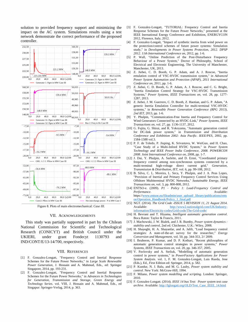
solution to provided frequency support and minimizing the impact on the AC system. Simulations results using a test network demonstrate the correct performance of the proposed controller.
100,080,060,040,020,00,0 [s]
160,50
158,00
155,50
153,00
150,50
148,00
Generator 31: Pgen in MW Case III
Generator 32: Pgen in MW Case III
148.9 MW
159.4 MW
100,080,060,040,020,00,0 [s]
232,50
230,00
227,50
225,00
222,50
220,00
Generator 1: Pgen in MW Case III
221.331 MW
221.2 MW
100,080,060,040,020,00,0 [s]
160,50
158,00
155,50
153,00
150,50
148,00
Generator 21: Pgen in MW Case III
Generator 22: Pgen in MW Case III
148.9 MW
159.3 MW
100,080,060,040,020,00,0 [s]
50,035
50,010
49,985
49,960
49,935
49,910
Bus 2: Freq in Hz Case III
50.01 Hz
DIg
SIL
EN
T
100,080,060,040,020,00,0 [s]
160,50
158,00
155,50
153,00
150,50
148,00
Generator 31: Pgen in MW Case III
Generator 32: Pgen in MW Case III
148.9 MW
159.4 MW
100,080,060,040,020,00,0 [s]
232,50
230,00
227,50
225,00
222,50
220,00
Generator 1: Pgen in MW Case III
221.331 MW
221.2 MW
100,080,060,040,020,00,0 [s]
160,50
158,00
155,50
153,00
150,50
148,00
Generator 21: Pgen in MW Case III
Generator 22: Pgen in MW Case III
148.9 MW
159.3 MW
100,080,060,040,020,00,0 [s]
50,035
50,010
49,985
49,960
49,935
49,910
Bus 2: Freq in Hz Case III
50.01 Hz
DIg
SIL
EN
T
100,080,060,040,020,00,0 [s]
-53,00
-57,00
-61,00
-65,00
-69,00
-73,00
Conv2: Pflow in MW Case III
-56.6 MW
-70.2 MW
100,080,060,040,020,00,0 [s]
-7,50
-10,00
-12,50
-15,00
-17,50
-20,00
OHL 1-2 /1: Pflow in MW Case III
-16.2 MW
-9.5 MW
100,080,060,040,020,00,0 [s]
-7,50
-10,00
-12,50
-15,00
-17,50
-20,00
OHL 1-2 /2: Pflow in MW Case III
-16.1 MW
-9.4 MW
100,080,060,040,020,00,0 [s]
-87,50
-90,00
-92,50
-95,00
-97,50
-100,00
Net interchange power: P in MW Case III
-88.9 MW
-89.1 MW
DIg
SIL
EN
T
Figure 8. Plots of main electromechanical: Case III.
VII. ACKNOWLEDGEMENTS
This study was partially supported in part by the Chilean
National Commission for Scientific and Technological
Research (CONICYT) and British Council under the
UKIERI, under grant Fondecyt 1130793 and
IND/CONT/E/13-14/700, respectively.
VIII. REFERENCES
[1] F. Gonzalez-Longatt, "Frequency Control and Inertial Response
Schemes for the Future Power Networks," in Large Scale Renewable
Power Generation, J. Hossain and A. Mahmud, Eds., ed: Springer
Singapore, 2014, pp. 193-231.
[2] F. Gonzalez-Longatt, "Frequency Control and Inertial Response
Schemes for the Future Power Networks," in Advances in Technologies
for Generation, Transmission and Storage, Green Energy and
Technology Series. vol. VIII, J. Hossain and A. Mahmud, Eds., ed
Singapur: Springer-Verlag, 2014, p. 363.
[3] F. Gonzalez-Longatt, "TUTORIAL: Frequency Control and Inertia
Response Schemes for the Future Power Networks," presented at the
IEEE Inernational Energy Conference and Exhibition, ENERGYCON
2012, Florence, Italy, 2012.
[4] F. Gonzalez-Longatt, "Impact of synthetic inertia from wind power on
the protection/control schemes of future power systems: Simulation
study," in Developments in Power Systems Protection, 2012. DPSP
2012. 11th International Conference on, 2012, pp. 1-6.
[5] P. Wall, "Online Prediction of the Post-Disturbance Frequency
Behaviour of a Power System," Doctor of Philosophy, School of
Electrical and Electronic Engineering, The University of Manchester,
Manchester, UK, 2013.
[6] Z. Jiebei, C. D. Booth, G. P. Adam, and A. J. Roscoe, "Inertia
emulation control of VSC-HVDC transmission system," in Advanced
Power System Automation and Protection (APAP), 2011 International
Conference on, 2011, pp. 1-6.
[7] Z. Jiebei, C. D. Booth, G. P. Adam, A. J. Roscoe, and C. G. Bright,
"Inertia Emulation Control Strategy for VSC-HVDC Transmission
Systems," Power Systems, IEEE Transactions on, vol. 28, pp. 1277-
1287, 2013.
[8] Z. Jiebei, J. M. Guerrero, C. D. Booth, Z. Haotian, and G. P. Adam, "A
generic Inertia Emulation Controller for multi-terminal VSC-HVDC
systems," in Renewable Power Generation Conference (RPG 2013),
2nd IET, 2013, pp. 1-6.
[9] Y. Phulpin, "Communication-Free Inertia and Frequency Control for
Wind Generators Connected by an HVDC-Link," Power Systems, IEEE
Transactions on, vol. 27, pp. 1136-1137, 2012.
[10] G. Fujita, G. Shirai, and R. Yokoyama, "Automatic generation control
for DC-link power system," in Transmission and Distribution
Conference and Exhibition 2002: Asia Pacific. IEEE/PES, 2002, pp.
1584-1588 vol.3.
[11] P. F. de Toledo, P. Jiuping, K. Srivastava, W. WeiGuo, and H. Chao,
"Case Study of a Multi-Infeed HVDC System," in Power System
Technology and IEEE Power India Conference, 2008. POWERCON
2008. Joint International Conference on, 2008, pp. 1-7.
[12] J. Dai, Y. Phulpin, A. Sarlette, and D. Ernst, "Coordinated primary
frequency control among non-synchronous systems connected by a
multi-terminal high-voltage direct current grid," Generation,
Transmission & Distribution, IET, vol. 6, pp. 99-108, 2012.
[13] B. Silva, C. L. Moreira, L. Seca, Y. Phulpin, and J. A. Peas Lopes,
"Provision of Inertial and Primary Frequency Control Services Using
Offshore Multiterminal HVDC Networks," Sustainable Energy, IEEE
Transactions on, vol. 3, pp. 800-808, 2012.
[14] ENTSO-e. (2009). P1 – Policy 1: Load-Frequency Control and
Performance. Available:
https://www.entsoe.eu/fileadmin/user_upload/_library/publications/ents
oe/Operation_Handbook/Policy_1_final.pdf
[15] NGT. (2014). The Grid Code -ISSUE 5 REVISION 11, 21 August 2014.
Available: http://www2.nationalgrid.com/UK/Industry-
information/Electricity-codes/Grid-code/The-Grid-code/
[16] H. Bevrani and T. Hiyama, Intelligent automatic generation control.
Boca Raton: Taylor & Francis, 2011.
[17] J. Machowski, J. W. Bialek, and J. R. Bumby, Power system dynamics :
stability and control, 2nd ed. Chichester, U.K.: Wiley, 2008.
[18] H. Shayeghi, H. A. Shayanfar, and A. Jalili, "Load frequency control
strategies: A state-of-the-art survey for the researcher," Energy
Conversion and Management, vol. 50, pp. 344-353, 2// 2009.
[19] I. Ibraheem, P. Kumar, and D. P. Kothari, "Recent philosophies of
automatic generation control strategies in power systems," Power
Systems, IEEE Transactions on, vol. 20, pp. 346-357, 2005.
[20] V. Pavlovsky and A. Steliuk, "Modelling of automatic generation
control in power systems," in PowerFactory Applications for Power
System Analysis. vol. 1, F. M. Gonzalez-Longatt, Luis Rueda, Jose
(Eds.), Ed., First Edition ed: Springer, 2014, p. 582.
[21] P. Kundur, N. J. Balu, and M. G. Lauby, Power system stability and
control. New York: McGraw-Hill, 1994.
[22] F. Milano, Power system modelling and scripting. London: Springer,
2010.
[23] F. Gonzalez-Longatt. (2014). IEEE 14 bus Test: Power system test case
archive. Available: http://fglongatt.org/OLD/Test_Case_IEEE_14.html


