
Gauge-origin invariant calculations of excitationenergies for molecules subject to strong magnetic
fields
Erik Tellgren
Center for Theoretical and Computational Chemistry, Department of Chemistry,University of Oslo, Norway
Workshop on Quantum Chemistry in Strong Magnetic Fields,September 13–14, 2010
Gauge-origin invariant calculations of excitationenergies (and geometrical gradients) for molecules
subject to strong magnetic fields
Erik Tellgren
Center for Theoretical and Computational Chemistry, Department of Chemistry,University of Oslo, Norway
Workshop on Quantum Chemistry in Strong Magnetic Fields,September 13–14, 2010
Gauge orig.inv., excitations, gradients. . . 2/35
Outline
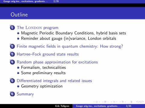
1 The London programMagnetic Periodic Boundary Conditions, hybrid basis setsReminder about gauge (in)variance, London orbitals
2 Finite magnetic fields in quantum chemistry: How strong?
3 Hartree–Fock ground state results
4 Random phase approximation for excitationsFormalism, technicalitiesSome preliminary results
5 Differentiated integrals and related issuesGeometry optimization
6 Summary
Erik Tellgren Gauge orig.inv., excitations, gradients. . . 2/35
Gauge orig.inv., excitations, gradients. . . 3/35
The London program
Magnetic Periodic Boundary Conditions, hybrid basis sets
From MPBC to mixed basis sets & London orbitals
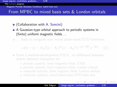
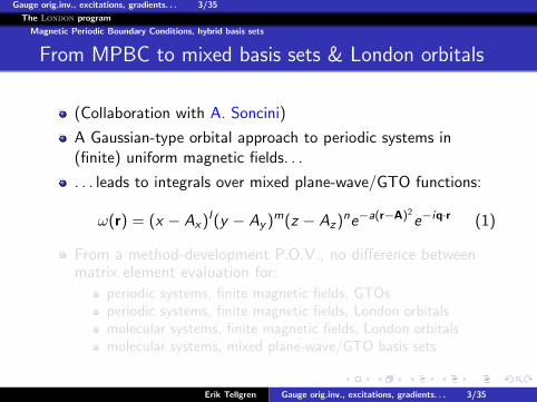
(Collaboration with A. Soncini)
A Gaussian-type orbital approach to periodic systems in(finite) uniform magnetic fields. . .
. . . leads to integrals over mixed plane-wave/GTO functions:
ω(r) = (x − Ax)l(y − Ay )m(z − Az)ne−a(r−A)2e−iq·r (1)
From a method-development P.O.V., no difference betweenmatrix element evaluation for:
periodic systems, finite magnetic fields, GTOsperiodic systems, finite magnetic fields, London orbitalsmolecular systems, finite magnetic fields, London orbitalsmolecular systems, mixed plane-wave/GTO basis sets
Erik Tellgren Gauge orig.inv., excitations, gradients. . . 3/35
Gauge orig.inv., excitations, gradients. . . 3/35
The London program
Magnetic Periodic Boundary Conditions, hybrid basis sets
From MPBC to mixed basis sets & London orbitals
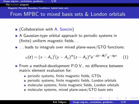
(Collaboration with A. Soncini)
A Gaussian-type orbital approach to periodic systems in(finite) uniform magnetic fields. . .
. . . leads to integrals over mixed plane-wave/GTO functions:
ω(r) = (x − Ax)l(y − Ay )m(z − Az)ne−a(r−A)2e−iq·r (1)
From a method-development P.O.V., no difference betweenmatrix element evaluation for:
periodic systems, finite magnetic fields, GTOsperiodic systems, finite magnetic fields, London orbitalsmolecular systems, finite magnetic fields, London orbitalsmolecular systems, mixed plane-wave/GTO basis sets
Erik Tellgren Gauge orig.inv., excitations, gradients. . . 3/35
Gauge orig.inv., excitations, gradients. . . 4/35
The London program
Magnetic Periodic Boundary Conditions, hybrid basis sets
From MPBC to mixed basis sets & London orbitals
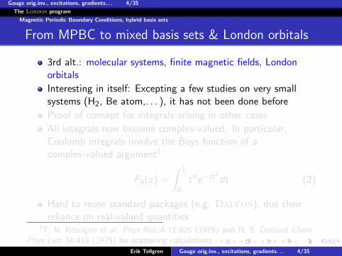
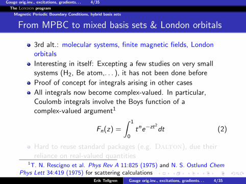
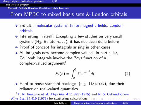
3rd alt.: molecular systems, finite magnetic fields, Londonorbitals
Interesting in itself: Excepting a few studies on very smallsystems (H2, Be atom,. . . ), it has not been done before
Proof of concept for integrals arising in other cases
All integrals now become complex-valued. In particular,Coulomb integrals involve the Boys function of acomplex-valued argument1
Fn(z) =
∫ 1
0tne−zt2
dt (2)
Hard to reuse standard packages (e.g. Dalton), due theirreliance on real-valued quantities
1T. N. Rescigno et al. Phys Rev A 11:825 (1975) and N. S. Ostlund ChemPhys Lett 34:419 (1975) for scattering calculations
Erik Tellgren Gauge orig.inv., excitations, gradients. . . 4/35
Gauge orig.inv., excitations, gradients. . . 4/35
The London program
Magnetic Periodic Boundary Conditions, hybrid basis sets
From MPBC to mixed basis sets & London orbitals
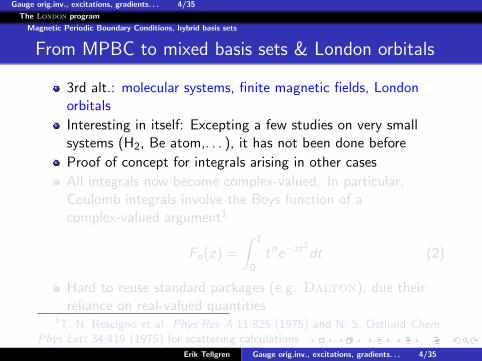
3rd alt.: molecular systems, finite magnetic fields, Londonorbitals
Interesting in itself: Excepting a few studies on very smallsystems (H2, Be atom,. . . ), it has not been done before
Proof of concept for integrals arising in other cases
All integrals now become complex-valued. In particular,Coulomb integrals involve the Boys function of acomplex-valued argument1
Fn(z) =
∫ 1
0tne−zt2
dt (2)
Hard to reuse standard packages (e.g. Dalton), due theirreliance on real-valued quantities
1T. N. Rescigno et al. Phys Rev A 11:825 (1975) and N. S. Ostlund ChemPhys Lett 34:419 (1975) for scattering calculations
Erik Tellgren Gauge orig.inv., excitations, gradients. . . 4/35
Gauge orig.inv., excitations, gradients. . . 5/35
The London program
Magnetic Periodic Boundary Conditions, hybrid basis sets
London orbitals: implementation issues
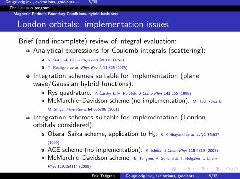
Brief (and incomplete) review of integral evaluation:
Analytical expressions for Coulomb integrals (scattering):N. Ostlund, Chem Phys Lett 34:419 (1975)
T. Rescigno et al. Phys Rev A 11:825 (1975)
Integration schemes suitable for implementation (planewave/Gaussian hybrid functions):
Rys quadrature: P. Carsky & M. Polasek, J Comp Phys 143:266 (1998)
McMurchie–Davidson scheme (no implementation): M. Tachikawa &
M. Shiga, Phys Rev E 64:056706 (2001)
Integration schemes suitable for implementation (Londonorbitals considered):
Obara–Saika scheme, application to H2: S. Kiribayashi et al. IJQC 75:637
(1999)
ACE scheme (no implementation): K. Ishida, J Chem Phys 118:4819 (2003)
McMurchie–Davidson scheme: E. Tellgren, A. Soncini & T. Helgaker, J Chem
Phys 129:154114 (2008)
Erik Tellgren Gauge orig.inv., excitations, gradients. . . 5/35
Gauge orig.inv., excitations, gradients. . . 6/35
The London program
Reminder about gauge (in)variance, London orbitals
London orbitals: A vs. B
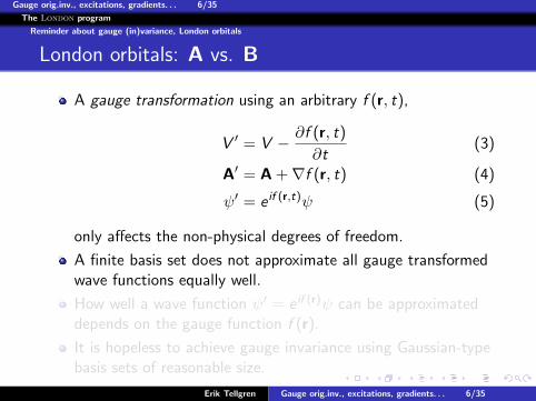
A gauge transformation using an arbitrary f (r, t),
V ′ = V − ∂f (r, t)
∂t(3)
A′ = A +∇f (r, t) (4)
ψ′ = e if (r,t)ψ (5)
only affects the non-physical degrees of freedom.
A finite basis set does not approximate all gauge transformedwave functions equally well.
How well a wave function ψ′ = e if (r)ψ can be approximateddepends on the gauge function f (r).
It is hopeless to achieve gauge invariance using Gaussian-typebasis sets of reasonable size.
Erik Tellgren Gauge orig.inv., excitations, gradients. . . 6/35
Gauge orig.inv., excitations, gradients. . . 6/35
The London program
Reminder about gauge (in)variance, London orbitals
London orbitals: A vs. B
A gauge transformation using an arbitrary f (r, t),
V ′ = V − ∂f (r, t)
∂t(3)
A′ = A +∇f (r, t) (4)
ψ′ = e if (r,t)ψ (5)
only affects the non-physical degrees of freedom.
A finite basis set does not approximate all gauge transformedwave functions equally well.
How well a wave function ψ′ = e if (r)ψ can be approximateddepends on the gauge function f (r).
It is hopeless to achieve gauge invariance using Gaussian-typebasis sets of reasonable size.
Erik Tellgren Gauge orig.inv., excitations, gradients. . . 6/35
Gauge orig.inv., excitations, gradients. . . 7/35
The London program
Reminder about gauge (in)variance, London orbitals
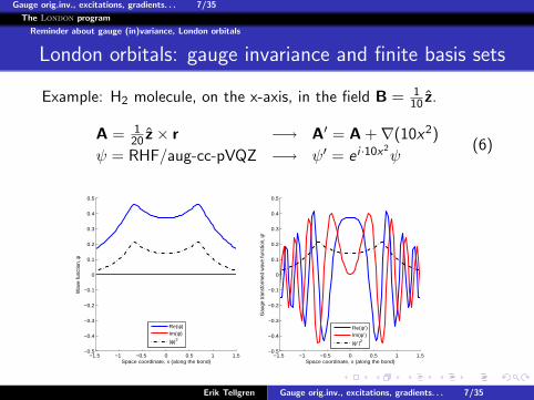
London orbitals: gauge invariance and finite basis sets
Example: H2 molecule, on the x-axis, in the field B = 110 z.
A = 120 z× r −→ A′ = A +∇(10x2)
ψ = RHF/aug-cc-pVQZ −→ ψ′ = e i ·10x2ψ
(6)
−1.5 −1 −0.5 0 0.5 1 1.5−0.5
−0.4
−0.3
−0.2
−0.1
0
0.1
0.2
0.3
0.4
0.5
Space coordinate, x (along the bond)
Wav
e fu
nctio
n, ψ
Re(ψ)Im(ψ)
|ψ|2
−1.5 −1 −0.5 0 0.5 1 1.5−0.5
−0.4
−0.3
−0.2
−0.1
0
0.1
0.2
0.3
0.4
0.5
Space coordinate, x (along the bond)
Gau
ge tr
ansf
orm
ed w
ave
func
tion,
ψ′
Re(ψ′)Im(ψ′)|ψ′|2
Erik Tellgren Gauge orig.inv., excitations, gradients. . . 7/35
Gauge orig.inv., excitations, gradients. . . 8/35
The London program
Reminder about gauge (in)variance, London orbitals
London orbitals: gauge invariance vs. gauge-origininvariance
Gauge invariance is not practically feasible with Gaussian basissets.
Restrict attention to uniform fields, fix some of the gaugefreedom by choosing ∇ · A = 0, and in addition take A to becylindrically symmetric.
A magnetic field B0 is then represented byA(r) = 1
2B0 × (r − G).
The gauge origin G contains the remaining gauge degrees offreedom.
More modest goal: make finite basis set calculationsindependent of the gauge origin G.
Erik Tellgren Gauge orig.inv., excitations, gradients. . . 8/35
Gauge orig.inv., excitations, gradients. . . 9/35
The London program
Reminder about gauge (in)variance, London orbitals
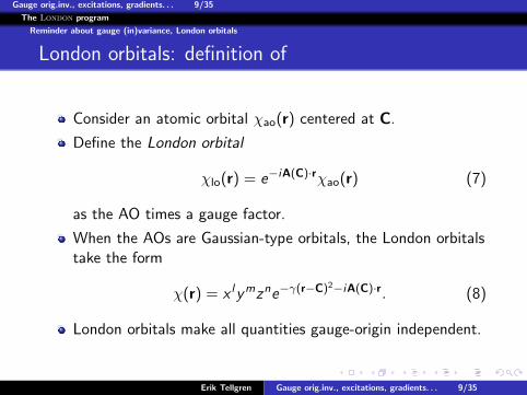
London orbitals: definition of
Consider an atomic orbital χao(r) centered at C.
Define the London orbital
χlo(r) = e−iA(C)·rχao(r) (7)
as the AO times a gauge factor.
When the AOs are Gaussian-type orbitals, the London orbitalstake the form
χ(r) = x lymzne−γ(r−C)2−iA(C)·r. (8)
London orbitals make all quantities gauge-origin independent.
Erik Tellgren Gauge orig.inv., excitations, gradients. . . 9/35
Gauge orig.inv., excitations, gradients. . . 10/35
The London program
Reminder about gauge (in)variance, London orbitals
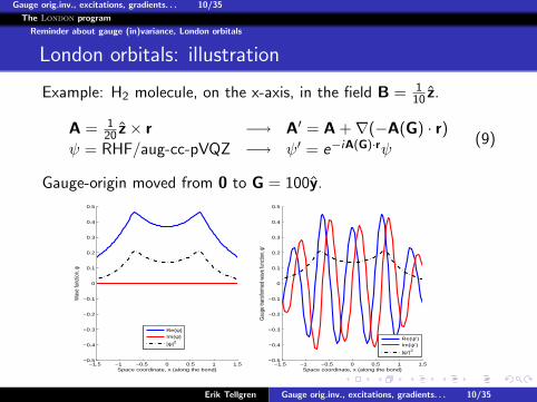
London orbitals: illustration
Example: H2 molecule, on the x-axis, in the field B = 110 z.
A = 120 z× r −→ A′ = A +∇(−A(G) · r)
ψ = RHF/aug-cc-pVQZ −→ ψ′ = e−iA(G)·rψ(9)
Gauge-origin moved from 0 to G = 100y.
−1.5 −1 −0.5 0 0.5 1 1.5−0.5
−0.4
−0.3
−0.2
−0.1
0
0.1
0.2
0.3
0.4
0.5
Space coordinate, x (along the bond)
Wav
e fu
nctio
n, ψ
Re(ψ)Im(ψ)
|ψ|2
−1.5 −1 −0.5 0 0.5 1 1.5−0.5
−0.4
−0.3
−0.2
−0.1
0
0.1
0.2
0.3
0.4
0.5
Space coordinate, x (along the bond)
Gau
ge tr
ansf
orm
ed w
ave
func
tion,
ψ′
Re(ψ′)Im(ψ′)|ψ′|2
Erik Tellgren Gauge orig.inv., excitations, gradients. . . 10/35
Gauge orig.inv., excitations, gradients. . . 11/35
The London program
Reminder about gauge (in)variance, London orbitals
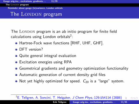
The London program
The London program is an ab initio program for finite fieldcalculations using London orbitals2:
Hartree-Fock wave functions [RHF, UHF, GHF].
DFT version?
Quite general integral evaluation
Excitation energies using RPA
Geometrical gradients and geometry optimization functionality
Automatic generation of current density grid files
Not yet highly optimized for speed. C20 is a “large” system.
2E. Tellgren, A. Soncini, T. Helgaker, J Chem Phys, 129:154114 (2008)Erik Tellgren Gauge orig.inv., excitations, gradients. . . 11/35
Gauge orig.inv., excitations, gradients. . . 12/35
Finite magnetic fields in quantum chemistry: How strong?
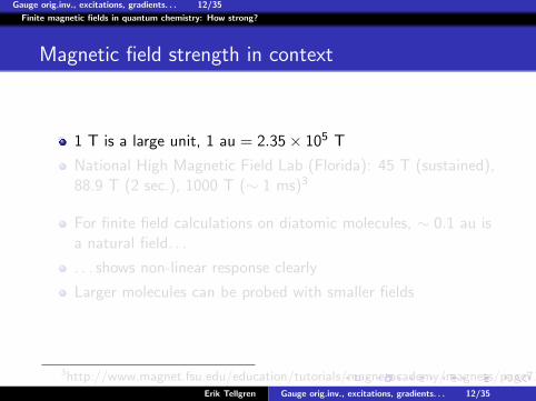
Magnetic field strength in context
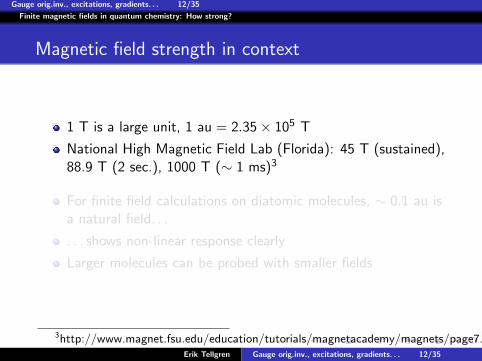
1 T is a large unit, 1 au = 2.35× 10⁵ T
National High Magnetic Field Lab (Florida): 45 T (sustained),88.9 T (2 sec.), 1000 T (∼ 1 ms)3
For finite field calculations on diatomic molecules, ∼ 0.1 au isa natural field. . .
. . . shows non-linear response clearly
Larger molecules can be probed with smaller fields
3http://www.magnet.fsu.edu/education/tutorials/magnetacademy/magnets/page7.htmlErik Tellgren Gauge orig.inv., excitations, gradients. . . 12/35
Gauge orig.inv., excitations, gradients. . . 12/35
Finite magnetic fields in quantum chemistry: How strong?
Magnetic field strength in context
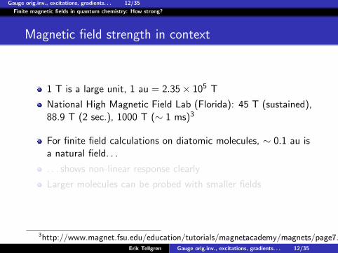
1 T is a large unit, 1 au = 2.35× 10⁵ T
National High Magnetic Field Lab (Florida): 45 T (sustained),88.9 T (2 sec.), 1000 T (∼ 1 ms)3
For finite field calculations on diatomic molecules, ∼ 0.1 au isa natural field. . .
. . . shows non-linear response clearly
Larger molecules can be probed with smaller fields
3http://www.magnet.fsu.edu/education/tutorials/magnetacademy/magnets/page7.htmlErik Tellgren Gauge orig.inv., excitations, gradients. . . 12/35
Gauge orig.inv., excitations, gradients. . . 12/35
Finite magnetic fields in quantum chemistry: How strong?
Magnetic field strength in context
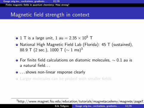
1 T is a large unit, 1 au = 2.35× 10⁵ T
National High Magnetic Field Lab (Florida): 45 T (sustained),88.9 T (2 sec.), 1000 T (∼ 1 ms)3
For finite field calculations on diatomic molecules, ∼ 0.1 au isa natural field. . .
. . . shows non-linear response clearly
Larger molecules can be probed with smaller fields
3http://www.magnet.fsu.edu/education/tutorials/magnetacademy/magnets/page7.htmlErik Tellgren Gauge orig.inv., excitations, gradients. . . 12/35
Gauge orig.inv., excitations, gradients. . . 12/35
Finite magnetic fields in quantum chemistry: How strong?
Magnetic field strength in context
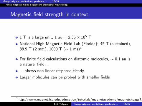
1 T is a large unit, 1 au = 2.35× 10⁵ T
National High Magnetic Field Lab (Florida): 45 T (sustained),88.9 T (2 sec.), 1000 T (∼ 1 ms)3
For finite field calculations on diatomic molecules, ∼ 0.1 au isa natural field. . .
. . . shows non-linear response clearly
Larger molecules can be probed with smaller fields
3http://www.magnet.fsu.edu/education/tutorials/magnetacademy/magnets/page7.htmlErik Tellgren Gauge orig.inv., excitations, gradients. . . 12/35
Gauge orig.inv., excitations, gradients. . . 12/35
Finite magnetic fields in quantum chemistry: How strong?
Magnetic field strength in context
1 T is a large unit, 1 au = 2.35× 10⁵ T
National High Magnetic Field Lab (Florida): 45 T (sustained),88.9 T (2 sec.), 1000 T (∼ 1 ms)3
For finite field calculations on diatomic molecules, ∼ 0.1 au isa natural field. . .
. . . shows non-linear response clearly
Larger molecules can be probed with smaller fields
3http://www.magnet.fsu.edu/education/tutorials/magnetacademy/magnets/page7.htmlErik Tellgren Gauge orig.inv., excitations, gradients. . . 12/35
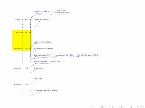
Earth magnetic field (30-50 microT)
fridge magnet
1 mT4.26e-9 au
field in sunspot
loud-speaker magnet medical MRI
1 T4.26e-6 au
500 MHz NMR spectro. (11.7 T)frog levitation exper. (16 T) strongest static field (45 T)
non-destructive pulse (88.9 T)
expl. pulsed fields (2.8 kT)
1 kT0.00426 au
neutron star, 1-100 MT
1 MT4.26 au
magnetar, up to 100 GTBrel = 4.41 GT,
cyclotron energy = mc^2
1 GT4260 au
Gauge orig.inv., excitations, gradients. . . 14/35
Hartree–Fock ground state results
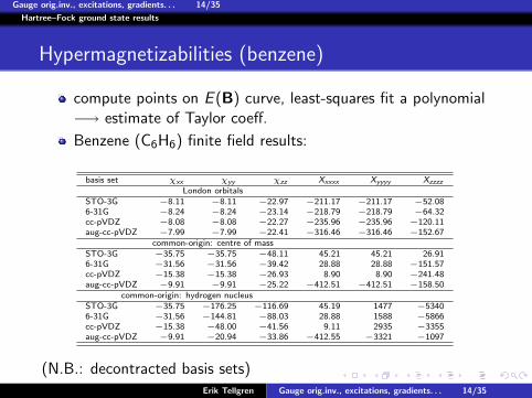
Hypermagnetizabilities (benzene)
compute points on E (B) curve, least-squares fit a polynomial−→ estimate of Taylor coeff.
Benzene (C6H6) finite field results:
basis set χxx χyy χzz Xxxxx Xyyyy Xzzzz
London orbitalsSTO-3G −8.11 −8.11 −22.97 −211.17 −211.17 −52.086-31G −8.24 −8.24 −23.14 −218.79 −218.79 −64.32cc-pVDZ −8.08 −8.08 −22.27 −235.96 −235.96 −120.11aug-cc-pVDZ −7.99 −7.99 −22.41 −316.46 −316.46 −152.67
common-origin: centre of massSTO-3G −35.75 −35.75 −48.11 45.21 45.21 26.916-31G −31.56 −31.56 −39.42 28.88 28.88 −151.57cc-pVDZ −15.38 −15.38 −26.93 8.90 8.90 −241.48aug-cc-pVDZ −9.91 −9.91 −25.22 −412.51 −412.51 −158.50
common-origin: hydrogen nucleusSTO-3G −35.75 −176.25 −116.69 45.19 1477 −53406-31G −31.56 −144.81 −88.03 28.88 1588 −5866cc-pVDZ −15.38 −48.00 −41.56 9.11 2935 −3355aug-cc-pVDZ −9.91 −20.94 −33.86 −412.55 −3321 −1097
(N.B.: decontracted basis sets)Erik Tellgren Gauge orig.inv., excitations, gradients. . . 14/35
Gauge orig.inv., excitations, gradients. . . 15/35
Hartree–Fock ground state results
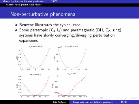
Non-perturbative phenomena
Benzene illustrates the typical caseSome paratropic (C4H4) and paramagnetic (BH, C20 ring)systems have slowly converging/diverging perturbationexpansions
−0.1 −0.05 0 0.05 0.10
0.02
0.04
0.06
0.08
0.1
∆ E
(B)
C6H
6, aug−cc−pVDZ
−0.1 −0.05 0 0.05 0.10
5
10
x 10−3
∆ E
(B)
C4H
4, aug−cc−pVDZ
0 0.1 0.2 0.3 0.40
0.01
0.02
0.03
0.04
0.05
0.06
∆ E
(B)
BH, aug−cc−pVTZ
0 0.01 0.02 0.03 0.04 0.05
−0.03
−0.02
−0.01
0
∆ E
(B)
C20
, cc−pVDZ
Erik Tellgren Gauge orig.inv., excitations, gradients. . . 15/35
Gauge orig.inv., excitations, gradients. . . 16/35
Hartree–Fock ground state results
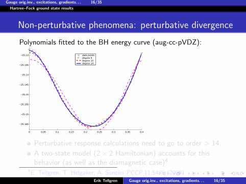
Non-perturbative phenomena: perturbative divergence
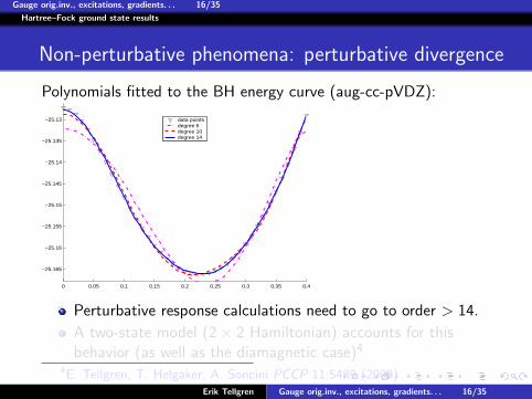
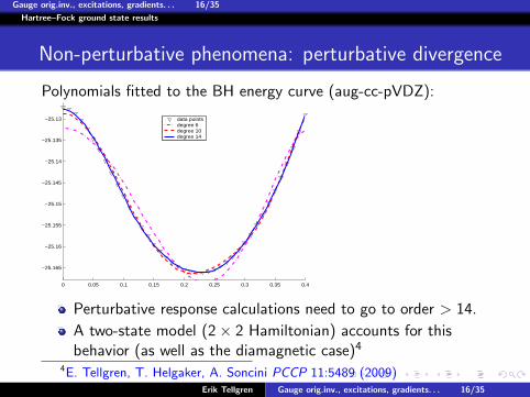
Polynomials fitted to the BH energy curve (aug-cc-pVDZ):
0 0.05 0.1 0.15 0.2 0.25 0.3 0.35 0.4
−25.165
−25.16
−25.155
−25.15
−25.145
−25.14
−25.135
−25.13 data pointsdegree 6degree 10degree 14
Perturbative response calculations need to go to order > 14.
A two-state model (2× 2 Hamiltonian) accounts for thisbehavior (as well as the diamagnetic case)4
4E. Tellgren, T. Helgaker, A. Soncini PCCP 11:5489 (2009)Erik Tellgren Gauge orig.inv., excitations, gradients. . . 16/35
Gauge orig.inv., excitations, gradients. . . 16/35
Hartree–Fock ground state results
Non-perturbative phenomena: perturbative divergence
Polynomials fitted to the BH energy curve (aug-cc-pVDZ):
0 0.05 0.1 0.15 0.2 0.25 0.3 0.35 0.4
−25.165
−25.16
−25.155
−25.15
−25.145
−25.14
−25.135
−25.13 data pointsdegree 6degree 10degree 14
Perturbative response calculations need to go to order > 14.
A two-state model (2× 2 Hamiltonian) accounts for thisbehavior (as well as the diamagnetic case)4
4E. Tellgren, T. Helgaker, A. Soncini PCCP 11:5489 (2009)Erik Tellgren Gauge orig.inv., excitations, gradients. . . 16/35
Gauge orig.inv., excitations, gradients. . . 17/35
Random phase approximation for excitations
Formalism, technicalities
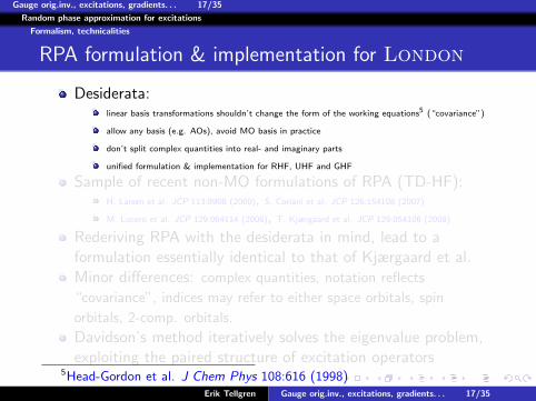
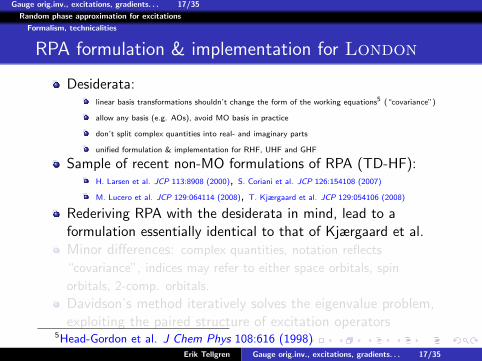
RPA formulation & implementation for London
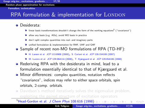
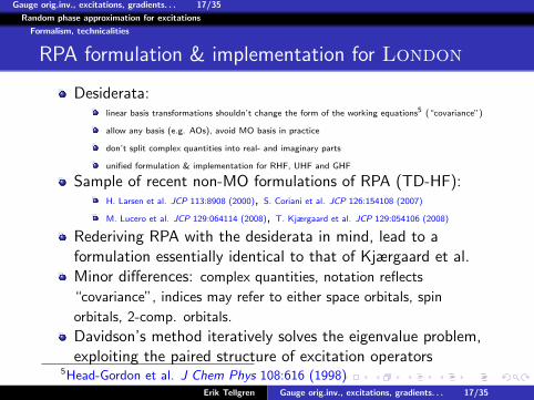
Desiderata:linear basis transformations shouldn’t change the form of the working equations5 (“covariance”)
allow any basis (e.g. AOs), avoid MO basis in practice
don’t split complex quantities into real- and imaginary parts
unified formulation & implementation for RHF, UHF and GHF
Sample of recent non-MO formulations of RPA (TD-HF):H. Larsen et al. JCP 113:8908 (2000), S. Coriani et al. JCP 126:154108 (2007)
M. Lucero et al. JCP 129:064114 (2008), T. Kjærgaard et al. JCP 129:054106 (2008)
Rederiving RPA with the desiderata in mind, lead to aformulation essentially identical to that of Kjærgaard et al.Minor differences: complex quantities, notation reflects
“covariance”, indices may refer to either space orbitals, spin
orbitals, 2-comp. orbitals.
Davidson’s method iteratively solves the eigenvalue problem,exploiting the paired structure of excitation operators
5Head-Gordon et al. J Chem Phys 108:616 (1998)Erik Tellgren Gauge orig.inv., excitations, gradients. . . 17/35
Gauge orig.inv., excitations, gradients. . . 17/35
Random phase approximation for excitations
Formalism, technicalities
RPA formulation & implementation for London
Desiderata:linear basis transformations shouldn’t change the form of the working equations5 (“covariance”)
allow any basis (e.g. AOs), avoid MO basis in practice
don’t split complex quantities into real- and imaginary parts
unified formulation & implementation for RHF, UHF and GHF
Sample of recent non-MO formulations of RPA (TD-HF):H. Larsen et al. JCP 113:8908 (2000), S. Coriani et al. JCP 126:154108 (2007)
M. Lucero et al. JCP 129:064114 (2008), T. Kjærgaard et al. JCP 129:054106 (2008)
Rederiving RPA with the desiderata in mind, lead to aformulation essentially identical to that of Kjærgaard et al.Minor differences: complex quantities, notation reflects
“covariance”, indices may refer to either space orbitals, spin
orbitals, 2-comp. orbitals.
Davidson’s method iteratively solves the eigenvalue problem,exploiting the paired structure of excitation operators
5Head-Gordon et al. J Chem Phys 108:616 (1998)Erik Tellgren Gauge orig.inv., excitations, gradients. . . 17/35
Gauge orig.inv., excitations, gradients. . . 18/35
Random phase approximation for excitations
Formalism, technicalities
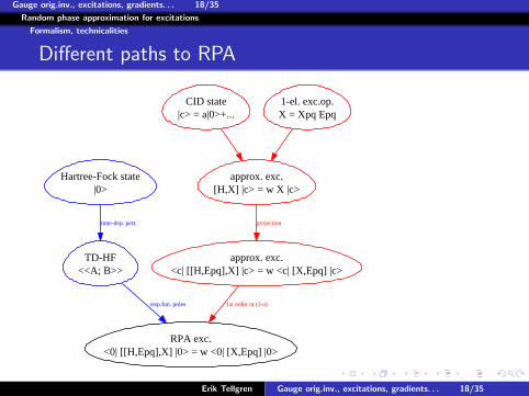
Different paths to RPA
Hartree-Fock state|0>
TD-HF<<A; B>>
time-dep. pert.
RPA exc.<0| [[H,Epq],X] |0> = w <0| [X,Epq] |0>
resp.fun. poles
CID state|c> = a|0>+...
approx. exc.[H,X] |c> = w X |c>
1-el. exc.op.X = Xpq Epq
approx. exc.<c| [[H,Epq],X] |c> = w <c| [X,Epq] |c>
projection
1st order in (1-a)
Erik Tellgren Gauge orig.inv., excitations, gradients. . . 18/35
Gauge orig.inv., excitations, gradients. . . 19/35
Random phase approximation for excitations
Formalism, technicalities
RPA formulation & implementation for London
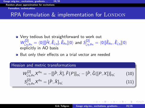
Very tedious but straightforward to work out
W[2]ζη,θκ = 〈0|[[H, Eζη], Eθκ]|0〉 and S
[2]ζη,θκ = 〈0|[Eθκ, Eζη]|0〉
explicitly in AO basis
But only their effects on a trial vector are needed
Hessian and metric transformations
W[2]ζη,θκX θκ = −[[P, X ], F (P)]ηζ − [P, G ([P,X ])]ηζ (10)
S[2]ζη,θκX θκ = [P, X ]ηζ (11)
Erik Tellgren Gauge orig.inv., excitations, gradients. . . 19/35
Gauge orig.inv., excitations, gradients. . . 20/35
Random phase approximation for excitations
Some preliminary results
RPA spectrum of boronmonohydride (BH)
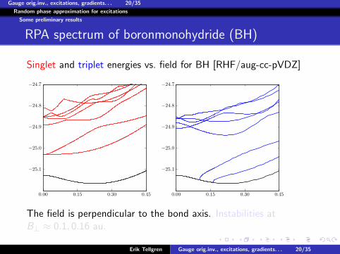
Singlet and triplet energies vs. field for BH [RHF/aug-cc-pVDZ]
0.00 0.15 0.30 0.45
−25.1
−25.0
−24.9
−24.8
−24.7
0.00 0.15 0.30 0.45
−25.1
−25.0
−24.9
−24.8
−24.7
The field is perpendicular to the bond axis. Instabilities atB⊥ ≈ 0.1, 0.16 au.
Erik Tellgren Gauge orig.inv., excitations, gradients. . . 20/35
Gauge orig.inv., excitations, gradients. . . 20/35
Random phase approximation for excitations
Some preliminary results
RPA spectrum of boronmonohydride (BH)
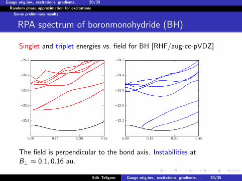
Singlet and triplet energies vs. field for BH [RHF/aug-cc-pVDZ]
0.00 0.15 0.30 0.45
−25.1
−25.0
−24.9
−24.8
−24.7
0.00 0.15 0.30 0.45
−25.1
−25.0
−24.9
−24.8
−24.7
The field is perpendicular to the bond axis. Instabilities atB⊥ ≈ 0.1, 0.16 au.
Erik Tellgren Gauge orig.inv., excitations, gradients. . . 20/35
Gauge orig.inv., excitations, gradients. . . 21/35
Random phase approximation for excitations
Some preliminary results
RPA spectrum of boronmonohydride (BH)
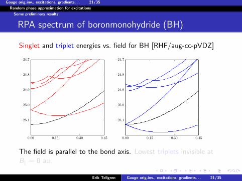
Singlet and triplet energies vs. field for BH [RHF/aug-cc-pVDZ]
0.00 0.15 0.30 0.45
−25.1
−25.0
−24.9
−24.8
−24.7
0.00 0.15 0.30 0.45
−25.1
−25.0
−24.9
−24.8
−24.7
The field is parallel to the bond axis. Lowest triplets invisible atB‖ = 0 au.
Erik Tellgren Gauge orig.inv., excitations, gradients. . . 21/35
Gauge orig.inv., excitations, gradients. . . 21/35
Random phase approximation for excitations
Some preliminary results
RPA spectrum of boronmonohydride (BH)
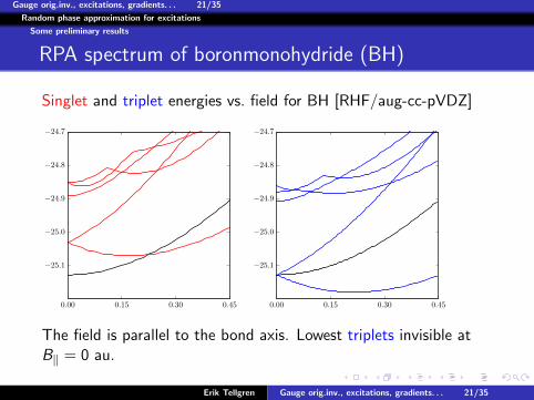
Singlet and triplet energies vs. field for BH [RHF/aug-cc-pVDZ]
0.00 0.15 0.30 0.45
−25.1
−25.0
−24.9
−24.8
−24.7
0.00 0.15 0.30 0.45
−25.1
−25.0
−24.9
−24.8
−24.7
The field is parallel to the bond axis. Lowest triplets invisible atB‖ = 0 au.
Erik Tellgren Gauge orig.inv., excitations, gradients. . . 21/35
Gauge orig.inv., excitations, gradients. . . 22/35
Random phase approximation for excitations
Some preliminary results
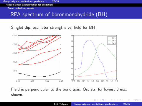
RPA spectrum of boronmonohydride (BH)
Singlet dip. oscillator strengths vs. field for BH
0.00 0.15 0.30 0.45
−25.1
−25.0
−24.9
−24.8
−24.7
0.00 0.05 0.10 0.15 0.20 0.25 0.30 0.35 0.40 0.450.00
0.05
0.10
0.15
0.20
0.25
0.30
0.35
0.40
Exc 1Exc 2Exc 3
Field is perpendicular to the bond axis. Osc.str. for lowest 3 exc.shown.
Erik Tellgren Gauge orig.inv., excitations, gradients. . . 22/35
Gauge orig.inv., excitations, gradients. . . 23/35
Random phase approximation for excitations
Some preliminary results
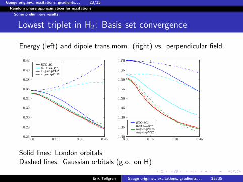
Lowest triplet in H2: Basis set convergence
Energy (left) and dipole trans.mom. (right) vs. perpendicular field.
0.00 0.15 0.30 0.450.26
0.28
0.30
0.32
0.34
0.36
0.38
0.40
0.42STO-3G6-311++G**aug-cc-pVDZaug-cc-pVTZ
0.00 0.15 0.30 0.451.30
1.35
1.40
1.45
1.50
1.55
1.60
1.65
1.70
STO-3G6-311++G**aug-cc-pVDZaug-cc-pVTZ
Solid lines: London orbitalsDashed lines: Gaussian orbitals (g.o. on H)
Erik Tellgren Gauge orig.inv., excitations, gradients. . . 23/35
Gauge orig.inv., excitations, gradients. . . 24/35
Random phase approximation for excitations
Some preliminary results
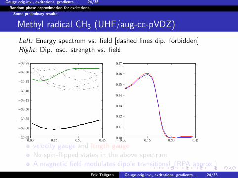
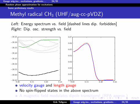
Methyl radical CH3 (UHF/aug-cc-pVDZ)
Left: Energy spectrum vs. field [dashed lines dip. forbidden]Right: Dip. osc. strength vs. field
0.00 0.15 0.30 0.45−39.65
−39.60
−39.55
−39.50
−39.45
−39.40
−39.35
−39.30
−39.25
0.00 0.15 0.30 0.450.00
0.01
0.02
0.03
0.04
0.05
0.06
0.07
velocity gauge and length gaugeNo spin-flipped states in the above spectrumA magnetic field modulates dipole transitions! (RPA approx.)
Erik Tellgren Gauge orig.inv., excitations, gradients. . . 24/35
Gauge orig.inv., excitations, gradients. . . 24/35
Random phase approximation for excitations
Some preliminary results
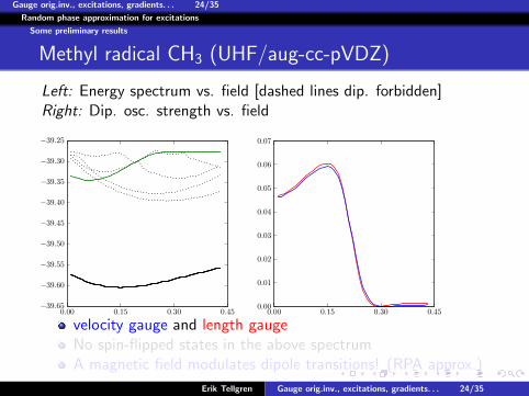
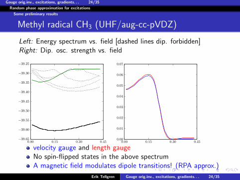
Methyl radical CH3 (UHF/aug-cc-pVDZ)
Left: Energy spectrum vs. field [dashed lines dip. forbidden]Right: Dip. osc. strength vs. field
0.00 0.15 0.30 0.45−39.65
−39.60
−39.55
−39.50
−39.45
−39.40
−39.35
−39.30
−39.25
0.00 0.15 0.30 0.450.00
0.01
0.02
0.03
0.04
0.05
0.06
0.07
velocity gauge and length gaugeNo spin-flipped states in the above spectrumA magnetic field modulates dipole transitions! (RPA approx.)
Erik Tellgren Gauge orig.inv., excitations, gradients. . . 24/35
Gauge orig.inv., excitations, gradients. . . 24/35
Random phase approximation for excitations
Some preliminary results
Methyl radical CH3 (UHF/aug-cc-pVDZ)
Left: Energy spectrum vs. field [dashed lines dip. forbidden]Right: Dip. osc. strength vs. field
0.00 0.15 0.30 0.45−39.65
−39.60
−39.55
−39.50
−39.45
−39.40
−39.35
−39.30
−39.25
0.00 0.15 0.30 0.450.00
0.01
0.02
0.03
0.04
0.05
0.06
0.07
velocity gauge and length gaugeNo spin-flipped states in the above spectrumA magnetic field modulates dipole transitions! (RPA approx.)
Erik Tellgren Gauge orig.inv., excitations, gradients. . . 24/35
Gauge orig.inv., excitations, gradients. . . 25/35
Differentiated integrals and related issues
Differentiated GTO integrals
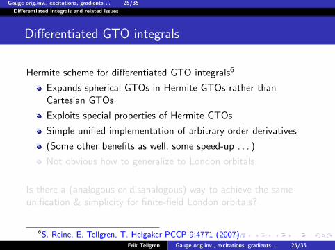
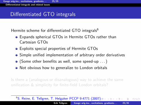
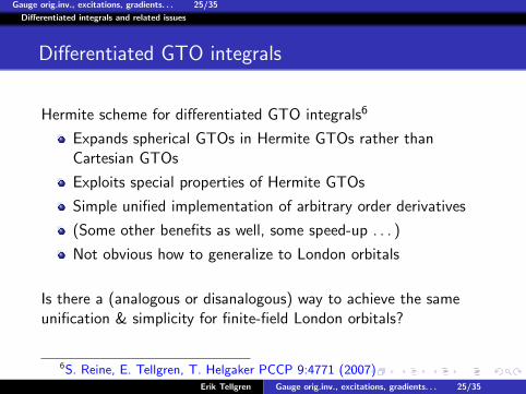
Hermite scheme for differentiated GTO integrals6
Expands spherical GTOs in Hermite GTOs rather thanCartesian GTOs
Exploits special properties of Hermite GTOs
Simple unified implementation of arbitrary order derivatives
(Some other benefits as well, some speed-up . . . )
Not obvious how to generalize to London orbitals
Is there a (analogous or disanalogous) way to achieve the sameunification & simplicity for finite-field London orbitals?
6S. Reine, E. Tellgren, T. Helgaker PCCP 9:4771 (2007)Erik Tellgren Gauge orig.inv., excitations, gradients. . . 25/35
Gauge orig.inv., excitations, gradients. . . 25/35
Differentiated integrals and related issues
Differentiated GTO integrals
Hermite scheme for differentiated GTO integrals6
Expands spherical GTOs in Hermite GTOs rather thanCartesian GTOs
Exploits special properties of Hermite GTOs
Simple unified implementation of arbitrary order derivatives
(Some other benefits as well, some speed-up . . . )
Not obvious how to generalize to London orbitals
Is there a (analogous or disanalogous) way to achieve the sameunification & simplicity for finite-field London orbitals?
6S. Reine, E. Tellgren, T. Helgaker PCCP 9:4771 (2007)Erik Tellgren Gauge orig.inv., excitations, gradients. . . 25/35
Gauge orig.inv., excitations, gradients. . . 26/35
Differentiated integrals and related issues
One approach to differentiated London orbitals
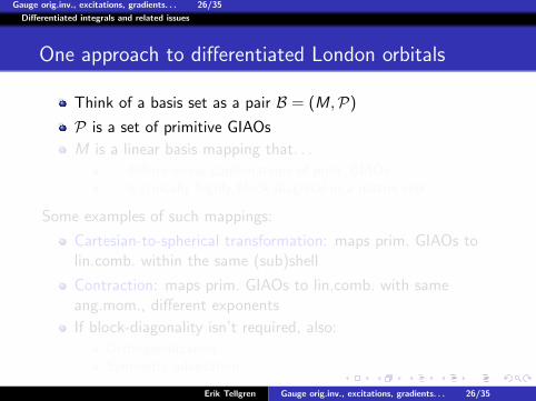
Think of a basis set as a pair B = (M,P)
P is a set of primitive GIAOs
M is a linear basis mapping that. . .
. . . defines linear combinations of prim. GIAOs
. . . is typically highly block diagonal in a matrix repr.
Some examples of such mappings:
Cartesian-to-spherical transformation: maps prim. GIAOs tolin.comb. within the same (sub)shell
Contraction: maps prim. GIAOs to lin.comb. with sameang.mom., different exponents
If block-diagonality isn’t required, also:
OrthogonalizationSymmetry adaptation
Erik Tellgren Gauge orig.inv., excitations, gradients. . . 26/35
Gauge orig.inv., excitations, gradients. . . 26/35
Differentiated integrals and related issues
One approach to differentiated London orbitals
Think of a basis set as a pair B = (M,P)
P is a set of primitive GIAOs
M is a linear basis mapping that. . .
. . . defines linear combinations of prim. GIAOs
. . . is typically highly block diagonal in a matrix repr.
Some examples of such mappings:
Cartesian-to-spherical transformation: maps prim. GIAOs tolin.comb. within the same (sub)shell
Contraction: maps prim. GIAOs to lin.comb. with sameang.mom., different exponents
If block-diagonality isn’t required, also:
OrthogonalizationSymmetry adaptation
Erik Tellgren Gauge orig.inv., excitations, gradients. . . 26/35
Gauge orig.inv., excitations, gradients. . . 27/35
Differentiated integrals and related issues
One approach to differentiated London orbitals
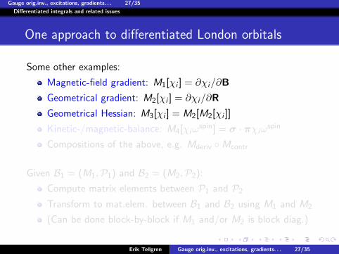
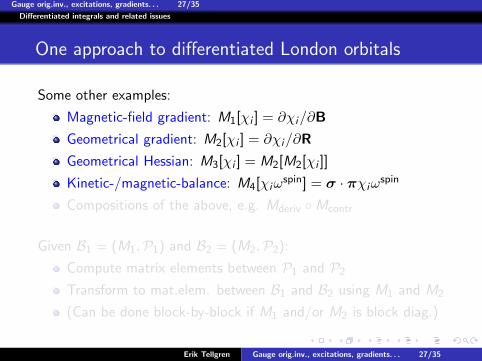
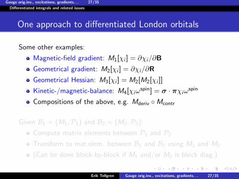
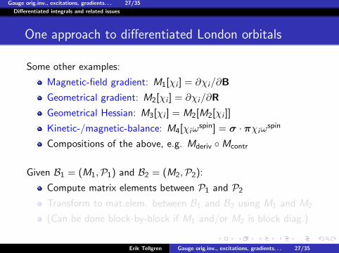
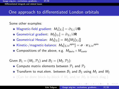
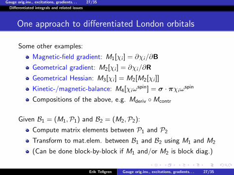
Some other examples:
Magnetic-field gradient: M1[χi ] = ∂χi/∂B
Geometrical gradient: M2[χi ] = ∂χi/∂R
Geometrical Hessian: M3[χi ] = M2[M2[χi ]]
Kinetic-/magnetic-balance: M4[χiωspin] = σ · πχiω
spin
Compositions of the above, e.g. Mderiv ◦Mcontr
Given B1 = (M1,P1) and B2 = (M2,P2):
Compute matrix elements between P1 and P2
Transform to mat.elem. between B1 and B2 using M1 and M2
(Can be done block-by-block if M1 and/or M2 is block diag.)
Erik Tellgren Gauge orig.inv., excitations, gradients. . . 27/35
Gauge orig.inv., excitations, gradients. . . 27/35
Differentiated integrals and related issues
One approach to differentiated London orbitals
Some other examples:
Magnetic-field gradient: M1[χi ] = ∂χi/∂B
Geometrical gradient: M2[χi ] = ∂χi/∂R
Geometrical Hessian: M3[χi ] = M2[M2[χi ]]
Kinetic-/magnetic-balance: M4[χiωspin] = σ · πχiω
spin
Compositions of the above, e.g. Mderiv ◦Mcontr
Given B1 = (M1,P1) and B2 = (M2,P2):
Compute matrix elements between P1 and P2
Transform to mat.elem. between B1 and B2 using M1 and M2
(Can be done block-by-block if M1 and/or M2 is block diag.)
Erik Tellgren Gauge orig.inv., excitations, gradients. . . 27/35
Gauge orig.inv., excitations, gradients. . . 28/35
Differentiated integrals and related issues
One approach to differentiated London orbitals
When higher-order derivatives/several basis sets are involved,another operation is useful:
Given B1 = (M1,P1) and B2 = (M2,P2), reexpress asB′1 = (M ′
1,P1 ∪ P2) and B′2 = (M ′2,P1 ∪ P2)
Mi [Pi ] = M ′i [P1 ∪ P2] =⇒ Bi ,B′i define the same basis
functions
Enables reuse of intermediate integrals (e.g. gradients for freewhen computing Hessians)
Erik Tellgren Gauge orig.inv., excitations, gradients. . . 28/35
Gauge orig.inv., excitations, gradients. . . 29/35
Differentiated integrals and related issues
Geometry optimization
Current status
Geometrical gradients have been implemented in Londonusing the above scheme
(When the density matrix response is available, it should alsobe easy to implement Hessians.)
BFGS geometry optimization implemented
works OK, but struggles to rotate molecules into optimalalignment with the external fieldneed to incorporate some extra coordinate that respondsdirectly to the total torquefor now, it’s best to provide an initial guess with the desiredalignment
Erik Tellgren Gauge orig.inv., excitations, gradients. . . 29/35
Gauge orig.inv., excitations, gradients. . . 30/35
Differentiated integrals and related issues
Geometry optimization
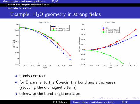
Example: H2O geometry in strong fields
0 0.02 0.04 0.06 0.08 0.1 0.12 0.14 0.1693.95
94
94.05
94.1
94.15
94.2
94.25
94.3
B [au]
d(O
−H
) [p
m]
H2O, HF/6−31G**
oopin−plane, ⊥ C2−axisin−plane, || C2−axis
0 0.02 0.04 0.06 0.08 0.1 0.12 0.14 0.16105.4
105.6
105.8
106
106.2
106.4
106.6
106.8
107
B [au]
H−
O−
H a
ngle
[deg
rees
]
H2O, HF/6−31G**
oopin−plane, ⊥ C2−axisin−plane, || C2−axis
bonds contract
for B parallel to the C2-axis, the bond angle decreases(reducing the diamagnetic term)
otherwise the bond angle increases
Erik Tellgren Gauge orig.inv., excitations, gradients. . . 30/35
Gauge orig.inv., excitations, gradients. . . 31/35
Differentiated integrals and related issues
Geometry optimization
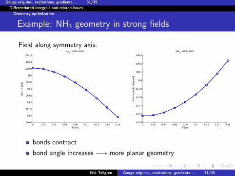
Example: NH3 geometry in strong fields
Field along symmetry axis:
0 0.02 0.04 0.06 0.08 0.1 0.12 0.14 0.1699.65
99.7
99.75
99.8
99.85
99.9
99.95
100
100.05
100.1
100.15
B [au]
d(N
−H
) [p
m]
NH3, HF/6−31G**
0 0.02 0.04 0.06 0.08 0.1 0.12 0.14 0.16107.5
107.6
107.7
107.8
107.9
108
108.1
108.2
108.3
B [au]
H−
N−
H a
ngle
[deg
rees
]
NH3, HF/6−31G**
bonds contract
bond angle increases −→ more planar geometry
Erik Tellgren Gauge orig.inv., excitations, gradients. . . 31/35
Gauge orig.inv., excitations, gradients. . . 32/35
Differentiated integrals and related issues
Geometry optimization
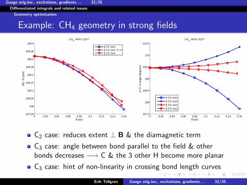
Example: CH4 geometry in strong fields
0 0.02 0.04 0.06 0.08 0.1 0.12 0.14 0.16107.95
108
108.05
108.1
108.15
108.2
108.25
108.3
108.35
108.4
B [au]
d(C
−H
) [p
m]
CH4, HF/6−31G**
|| C2−axis|| C3−axis, C−H|| C3−axis
0 0.02 0.04 0.06 0.08 0.1 0.12 0.14 0.16107.5
108
108.5
109
109.5
110
110.5
B [au]
H−
C−
H a
ngle
[deg
rees
]
CH4, HF/6−31G**
|| C2−axis|| C2−axis|| C3−axis|| C3−axis
C2 case: reduces extent ⊥ B & the diamagnetic term
C3 case: angle between bond parallel to the field & otherbonds decreases −→ C & the 3 other H become more planar
C3 case: hint of non-linearity in crossing bond length curves
Erik Tellgren Gauge orig.inv., excitations, gradients. . . 32/35
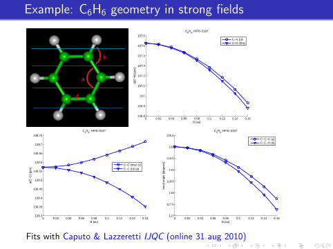
Example: C6H6 geometry in strong fields
0 0.02 0.04 0.06 0.08 0.1 0.12 0.14 0.16106.8
106.9
107
107.1
107.2
107.3
107.4
107.5
107.6
B [au]
d(C
−H
) [p
m]
C6H
6, HF/6−31G*
C−H || BC−H other
0 0.02 0.04 0.06 0.08 0.1 0.12 0.14 0.16138.3
138.35
138.4
138.45
138.5
138.55
138.6
138.65
138.7
138.75
B [au]
d(C
−C
) [p
m]
C6H
6, HF/6−31G*
C−C other (c)C−C || B (d)
0 0.02 0.04 0.06 0.08 0.1 0.12 0.14 0.16117
117.5
118
118.5
119
119.5
120
120.5
B [au]
bond
ang
le [d
egre
es]
C6H
6, HF/6−31G*
C−C−C (a)C−C−H (b)
Fits with Caputo & Lazzeretti IJQC (online 31 aug 2010)
Gauge orig.inv., excitations, gradients. . . 34/35
Summary
Summary
London opens up for several applications, from analternative method to compute static response properties toinvestigation of intrinsically non-perturbative phenomena
Functionality for RPA excitations recently added
AO-/arbitrary basis formulationunified handling of RHF/UHF/GHF
Functionality related to gradients recently added
part of quite simple & general scheme for derivativesBFGS geometry optimizeropens up for Hessians, 4-component integrals
Future goals include
Correlation: CI, etc.Study of CDFT functionals using Adiabatic Connectionmethods (with A. Teale)
Erik Tellgren Gauge orig.inv., excitations, gradients. . . 34/35
Gauge orig.inv., excitations, gradients. . . 35/35
Acknowledgments
Thanks to. . .
Trygve Helgaker
Alessandro Soncini
Kai Kaarvann Lange (master student working on the RPAimplementation)
Pawe l Sa lek, Simen Reine
The audience
Erik Tellgren Gauge orig.inv., excitations, gradients. . . 35/35


