

Gene Shaving – Applying PCA
• Identify groups of genes a set of genes using PCA which serve as the informative genes to classify samples.
• The “gene shaving” method is also a method of clustering genes and sample cells. But unlike classic clustering, in this method, one gene could belong to more than one cluster.
Features of Gene Groups• The genes in each cluster behave in a similar
manner, which suggests similar or related function among genes;
• The cluster centroid shows high variance across the samples, which indicates the potential of this cluster to distinguish sample classes;
• The groups are as much uncorrelated between each other (which encourages seeking groups of different specification) as possible.

Motivation and Details
• We favor subsets of genes that
– All behave in a similar manner (coherence)
– And all show large across the cell lines.
• Given an expression array, we seek a sequence
of nested gene clusters of size k. has the
property that the variance of the cluster mean
is maximum over all clusters of size k.
kS
kS

Gene Shaving approach finds the linear combination of genes having maximal variation among samples. This linear combination of genes is viewed as a “super gene”.
The genes having lowest correlation with the “super gene” is removed (shaved). The process is continued until the subset of genes contains only one gene.
This process produces a sequence of gene blocks, each containing genes that are similar to one another and displaying large variance across samples.A statistical approach
Identifies subsets of genes with coherent expression patterns and large variation across conditions
Gene may belong to more than one cluster
Can be either un-supervised or supervised

Gene Shaving Algorithm-1• STEP 1. Start with the entire expression data X,
each row centered to have zero mean.
• STEP 2. Compute the leading principal component
of the rows of X.
• STEP 3. Shave off the proportion alpha (typically
10%) of the rows having smallest inner-product
with the leading principal component.
• STEP 4. Repeat step 2 and 3 until only one gene
remains.

Gene Shaving Iteration

Gene Shaving Algorithm-2
• STEP 5. This produces a sequence of nested gene clusters
where denotes a cluster of k genes. Estimate the
optimal cluster size
• STEP 6. Orthogonalize each row of X with respect to ,
the average gene in
• STEP 7. Repeat steps 1-5 above with the orthogonalized
data, to find the second optimal cluster. This process is
continued until a maximum of M clusters are found, with
M chosen apriori.
121
SSSS kkN
kS
x
k̂
kS ˆ

Principal Component of the rows
slides
genesslides
genes
Derive the first principal component Z1
Z1slide
Super-gene

The Gap estimate of cluster size
2
1
)(1
xxp
p
jj
(Vt) Variance Total
)(V VarianceBetween 1002 b
R
sequence ofmember th for the measures the 2 kRDk
XX b ofmatrix data permuted a* *b
k
2* cluster for measures the SRD b
k
BbDD b
k
b
k ,,1over of average the ** *)Gap(function Gap The kk DDk
We then select as the optimal number of genes that value k producingThe largest gap:
)Gap(argmaxˆ kk k )Gap(argmaxˆ kk k
Vb =2
1
)(1
kSi
p
jij xx
kpVt =

Gene Shaving (Cont.)
The first three gene clusters found for the DLCL data
Gene Shaving (Cont.)
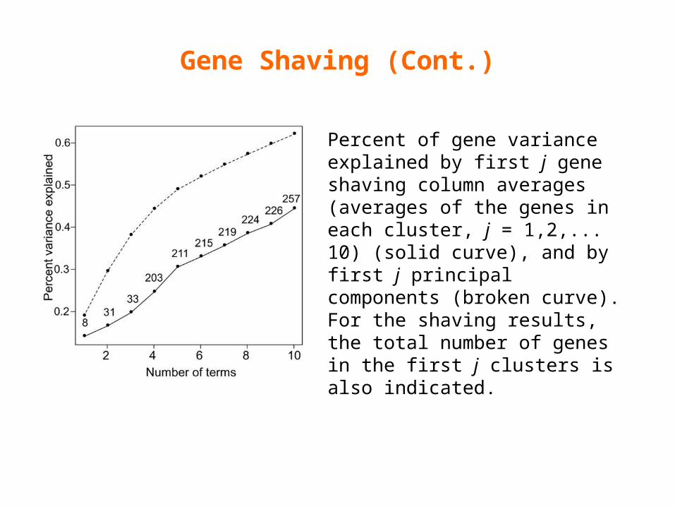
Percent of gene variance explained by first j gene shaving column averages (averages of the genes in each cluster, j = 1,2,... 10) (solid curve), and by first j principal components (broken curve). For the shaving results, the total number of genes in the first j clusters is also indicated.

Gene Shaving ( Cont.)
a) Variance plots for real and randomized data. The percent variance explained by each cluster, both for the original data, and for an average over three randomized versions.
b) Gap estimates of cluster size. The gap curve, which highlights the difference between the pair of curves, is shown.

References
• ‘Gene Shaving’ as a method for identifying distinct sets of genes with similar expression patterns T. Hastie, R. Tibshirani, M.B. Eisen, A Alizadeh, R. Levy,L Staudt, W.C Chan, D.Botstein and P. Brown. Genome Biology 2000. http://genomebiology.com/2000/1/2/research/0003/#B14.


