IFPRI Discussion Paper 00900

September 2009

Greenhouse Gas Mitigation

Issues for Indian Agriculture

Gerald C. Nelson Richard Robertson

Siwa Msangi Tingju Zhu Xiaoli Liao

Puja Jawajar

Environment and Production Technology Division

ii

INTERNATIONAL FOOD POLICY RESEARCH INSTITUTE The International Food Policy Research Institute (IFPRI) was established in 1975. IFPRI is one of 15 agricultural research centers that receive principal funding from governments, private foundations, and international and regional organizations, most of which are members of the Consultative Group on International Agricultural Research (CGIAR).

FINANCIAL CONTRIBUTORS AND PARTNERS IFPRI’s research, capacity strengthening, and communications work is made possible by its financial contributors and partners. IFPRI gratefully acknowledges generous unrestricted funding from Australia, Canada, China, Denmark, Finland, France, Germany, India, Ireland, Italy, Japan, the Netherlands, Norway, the Philippines, Sweden, Switzerland, the United Kingdom, the United States, and the World Bank.

AUTHORS Gerald C. Nelson, International Food Policy Research Institute Senior Research Fellow, Environment and Production Technology Division Email: g.nelson@cgiar.org Richard Robertson, International Food Policy Research Institute Research Fellow, Environment and Production Technology Division Siwa Msangi, International Food Policy Research Institute Senior Research Fellow, Environment and Production Technology Division Tingju Zhu, International Food Policy Research Institute Scientist, Environment and Production Technology Division Xiaoli Liao, University of Illinois at Urbana-Champaign PhD student, Department of Agricultural and Consumer Economics Puja Jawajar, Independent Consultant

Notices 1 Effective January 2007, the Discussion Paper series within each division and the Director General’s Office of IFPRI were merged into one IFPRI–wide Discussion Paper series. The new series begins with number 00689, reflecting the prior publication of 688 discussion papers within the dispersed series. The earlier series are available on IFPRI’s website at www.ifpri.org/pubs/otherpubs.htm#dp. 2 IFPRI Discussion Papers contain preliminary material and research results. They have not been subject to formal external reviews managed by IFPRI’s Publications Review Committee but have been reviewed by at least one internal and/or external reviewer. They are circulated in order to stimulate discussion and critical comment.

Copyright 2008 International Food Policy Research Institute. All rights reserved. Sections of this material may be reproduced for personal and not-for-profit use without the express written permission of but with acknowledgment to IFPRI. To reproduce the material contained herein for profit or commercial use requires express written permission. To obtain permission, contact the Communications Division at ifpri-copyright@cgiar.org.

iii

Contents Executive Summary vi

1. Introduction 1

2. Agriculture’s Role in Greenhouse Gas Emissions and Mitigation 2

3. Assumptions and Data Sources 3

4. Effects of Midseason Drying on Methane Emissions 14

5. Effects of Fertilizer Type on N2O Emissions 17

6. Emissions of CO2 from Groundwater Pumping 18

7. Carbon Sequestration Supply Curves and Efficiency of Payment Schemes 22

8. Conclusions 27

Technical Appendix A: N2O Determinants 28

Technical Appendix B: IPCC N2O Methodology 31

Technical Appendix C: India Fertilizer Use Projections 33

Technical Appendix D: Estimating the Contribution of Groundwater Irrigation Pumping to CO2 Emissions 37

References 47

Recent IFPRI Discussion Papers 48

List of Tables

Table 1. Greenhouse gas emissions, 2004 estimates (million mt, CO2e) 1

Table 2. Global warming potential (CO2e) 2

Table 3. Decision tree to allocate GLC 2000 and ISAM data to 1 km pixels 4

Table 4. Sensitivity analysis for different rates of N application, water regimes, and manure application affecting simulated rice yields, N uptake, and annual GHG emissions. 7

Table 5. Assumptions about GHG emissions and mitigation 8

Table 6. India carbon pool estimates, 2000 (million mt C) 10

Table 7. India agricultural GHG emissions, 2000 and 2050 (million mt CO2e, IPCC assumptions unless otherwise noted) 10

Table 8. Trade unit values, average of 2001–2003 12

Table 9. Effects of midseason drying on irrigated-rice GHG emissions, 2000–2050. 15

Table 10. Irrigation water use by source, 2000–2050 19

Table 11. Carbon emissions from Indian groundwater pumping for irrigation, four scenarios (million mt, CO2e) 20

iv

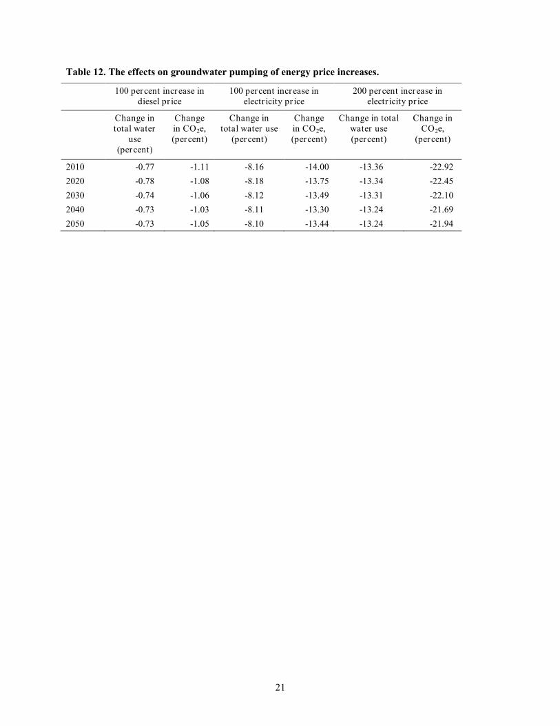
Table 12. The effects on groundwater pumping of energy price increases. 21

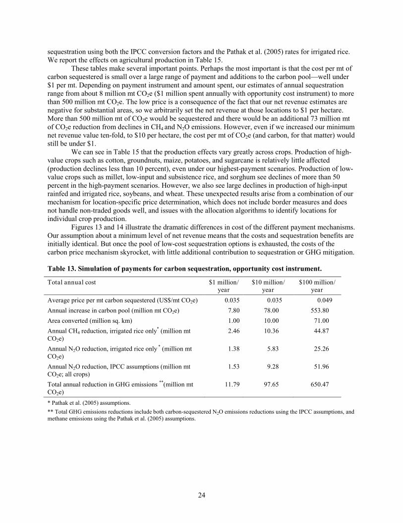
Table 13. Simulation of payments for carbon sequestration, opportunity cost instrument. 24

Table 14. Simulation of payments for carbon sequestration, carbon price instrument. 25

Table 15. Share of total production lost with different instruments (percent). 26

Table A.1. Summary statistics of variables. 28

Table A.2. Regression results, determinants of N2O emissions. 30

Table C1: Nutrient use by crop and management (kg/ha) 33

Table C2. Lookup table IMPACT crops and FAO crops. 34

Table C3. IMPACT production projections by crop, 2000-2050 (000 mt). 35

Table C4. India fertilizer use projections, 2000-2050 (million mt nutrient). 35

Table D1. CO2 emissions from Indian power plants 38

Table D2. Effective Efficiency of Indian Irrigation (liters consumed/liters pumped) 38

Table D3. Reference crop evapotranspiration rates for Indian FPUs (mm/hectare) 40

Table D4. Tubewell count, by state and type and area irrigated, 2000 41

Table D5. Irrigation water use by source, 2000-2050. 43

Table D6. Sensitivity analysis assumptions 43

Table D7. Carbon emissions from Indian groundwater pumping for irrigation, three scenarios (000 mt, C). 44

List of Figures

Figure 1. FPUs in India and neighboring countries. 5

Figure 2. Changes in soil carbon for different cropping systems, Futchimiram, Nigeria 6

Figure 3. Changes in soil carbon for different cropping systems, Lingampally village, India 6

Figure 4. Nitrogen yield curve, irrigated rice (Pathak et al. 2005) . 7

Figure 5. Methane emissions, irrigated rice (Pathak et al. 2005) 7

Figure 6. Carbon pool, above and below ground (mt C/ha) 11

Figure 7. CO2e from CH4 and N2O emissions from rice using Pathak et al. (2005) assumptions (CO2e mt/ha) 11

Figure 8. Location-specific milled rice prices based on export unit values (US$/mt). 12

Figure 9. Location-specific maize prices based on import unit values (US$/mt). 12

Figure 10. Estimated net revenue per hectare per year for irrigated rice (US$/ha). 13

Figure 11. Locations of changes in GHG emissions with midseason drying, 2000 (change in mt CO2e/ha/year). 16

v

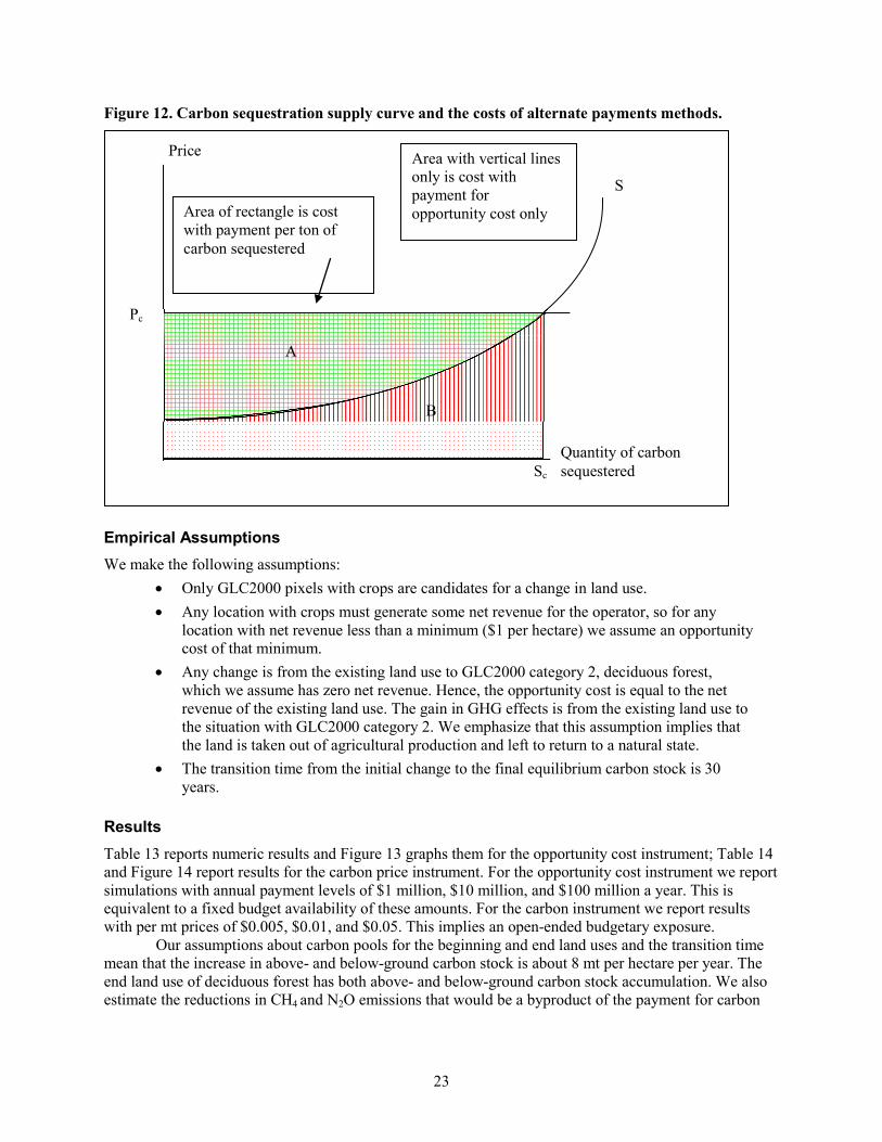
Figure 12. Carbon sequestration supply curve and the costs of alternate payments methods. 23

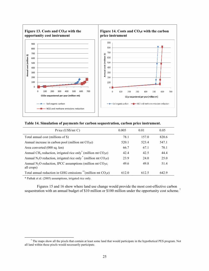
Figure 13. Costs and CO2e with the opportunity cost instrument 25

Figure 14. Costs and CO2e with the carbon price instrument 25

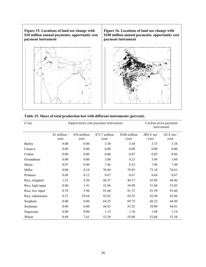
Figure 15. Locations of land use change with $10 million annual payments, opportunity cost payment instrument 26

Figure 16. Locations of land use change with $100 million annual payments, opportunity cost payment instrument 26

Figure D1. Effective Efficiency of Indian Irrigation. 39

vi

EXECUTIVE SUMMARY

By some estimates, agricultural practices account for 20 percent of India’s total greenhouse gas (GSG) emissions; thus, cost-effective reductions in agricultural emissions could significantly lower India’s overall emissions.

We explore mitigation options for three agricultural sources of GHGs—methane (CH4) emissions from irrigated rice production, nitrous oxide (N2O) emissions from the use of nitrogenous fertilizers, and the release of carbon dioxide (CO2) from energy sources used to pump groundwater for irrigation. We also examine how changes in land use would affect carbon sequestration. Although livestock-based methane emissions may be significant, we do not include them here, both because the data on livestock numbers and emissions are inadequate and technologies to reduce emissions are in early stages of development. We find great opportunities for cost-effective mitigation of GHGs in Indian agriculture, but caution that our results are based on a variety of data sources, some of which are of poor quality.

Emissions Estimates for 2000 and 2050 Using the International Food Policy Research Institute’s IMPACT model, we estimate emissions

today and in 2050, in carbon dioxide equivalent (CO2e) units. Raising crops results in N2O emissions from the use of nitrogenous fertilizers and CH4 emissions from anaerobic decomposition of organic material typically associated with flooded irrigation techniques. In addition, groundwater pumping releases small amounts of CO2 dissolved in water and much larger amounts from the energy sources used to lift the water to the surface.

Overall, N2O emissions from all crop agriculture are the largest source of GHG emissions. This result is based on a straightforward application of the Intergovernmental Panel on Climate Change’s (IPCC) standard accounting methodology, which is subject to great uncertainty (see Technical Appendix B: IPCC N2O Methodology). We also use results from a study by Bhati et al. (2004) that are based on actual field estimates for irrigated rice. Using Bhati et al. (2004), N2O emissions from irrigated rice were 26.9 million metric tonnes (mt) CO2e in 2000 and will increase to 34.5 million mt CO2e in 2050. Using the IPPC methodology, estimates of N2O emissions are much lower; only 4.5 million mt CO2e in 2000 and 5.8 million mt CO2e in 2050. For all other crops, the IPCC methodology results in an estimated 85.5 million mt CO2e emissions in 2000, increasing to 97.2 million mt CO2e in 2050 (Table 7).

Focusing on groundwater pumping for irrigated rice, we find the resulting emissions from use of coal-fired electricity and diesel fuel are large, with an estimated release of 58.7 million mt CO2e in 2000. Of this total, 95 percent comes from electric pumps using coal-fired generation. The remaining 5 percent is released by diesel-powered pumps (Table 11). Deep wells powered by electricity are the single largest source of CO2 emissions from groundwater pumping. They account for 65 percent of the total in 2000 and 87 percent in 2050, as we assume most of the increase in irrigation water is supplied by deep wells. Finally, CH4 emissions from irrigated rice are substantial, with 47.8 million mt CO2e in 2000, increasing to 61.3 million mt CO2e in 2050 (Table 7).

By combining these results, our estimate of the total CO2e from these sources in 2000 is 148.7 to 218.9 million mt CO2e. Total Indian GHG emissions reported by the World Resources Institute (cait.wri.org) in 2004 are 1,853 million mt CO2e; agricultural emissions are 375 million mt CO2e. Thus, our estimates for these agricultural activities range from 8.0 to 11.8 percent of total GHG emissions and from 39.6 to 58.4 percent of agricultural GHG emissions. We estimate that, without mitigation policies and programs, these sources will contribute 237.6 to 327.7 million mt CO2e in 2050.

Estimating the Opportunity Costs of Mitigation Options The next step is estimating the opportunity costs of various mitigation options. We explore these

options: changing irrigation management techniques for irrigated rice, changing the fertilizer type, raising

vii

the price of energy sources used in pumping groundwater, and paying farmers to adopt carbon sequestering management techniques.

Methane emissions. Methane emissions from irrigated rice can be reduced by temporarily draining the field during the growing period to allow aerobic decomposition. We estimate that with a single midseason drying, annual methane emissions would drop by about 18 percent with only a 1.5 percent yield decline. By contrast, with “business as usual,” the CO2e from methane would increase by almost 25 percent by 2050 as production rises (Table 9). Implementing midseason drying on all irrigated rice areas would stabilize methane emissions at 2000 levels even as production grows substantially. The opportunity cost of the yield decline is about 4.4 percent of net revenue (or about $213 million in 2000), but not all areas are affected equally, as Figure 11 shows. The lost revenue could potentially be made up by environmental service payments funded from the global carbon market.

N2O emissions. Our analysis of the effects of fertilizer type on N2O emissions has results that are similar to those used in the IPCC methodology. There are some promising indications that fertilizer type and crop choice influence N2O emissions, but the statistical results are not strong enough to warrant empirical estimates. We are not able to provide quantitative estimates of the potential benefits of extension efforts in encouraging efficiency of fertilizer use, use of biofertilizers, manure management, and use of compost from agricultural and domestic waste programs, although such efforts would likely be important.

CO2 emissions from groundwater pumping. Groundwater pumping requires energy and most of that energy in India comes from electricity generated from coal. A much smaller share uses diesel-powered pumps. We simulate the effects on water use and food production of a 100 percent increase in the price of diesel and 100 and 200 percent increases in the price of electricity (Table 12). A 100 percent increase in the diesel price reduces total water use by less than 1 percent and CO2e emissions by slightly more than 1 percent. However, a 100 percent increase in the electricity price charged to the rural sector reduces water use by more than 8 percent and CO2e emissions by 14 percent. There is almost no effect on crop production. In essence, the cost of the electricity price increase would be borne by farmers. It is likely that such a price increase would encourage adoption of more efficient water use practices, but we are not able to capture that in our modeling.

Pump efficiency has a substantial impact on estimated CO2 emissions. Our baseline assumption is 30 percent energy use efficiency in both diesel and electric pumps. If pump efficiency is instead 20 percent, CO2 emissions increase by 50 percent. Any technological improvements in pump efficiency would result in substantially lower emissions.

Environmental service payments to sequester carbon above and below ground. Changes in agricultural practices can increase carbon sequestered above and below ground, but might reduce farmer incomes. We analyzed the potential for using environmental service payments and where the most cost-effective locations would be, considering both an opportunity cost instrument (pay farmers just the opportunity cost of revenue foregone from adopting the sequestration practice) and a fixed-price-of-carbon instrument (pay farmers for every ton of carbon sequestered).

Perhaps the most important result is that the cost per mt of carbon sequestered is small over a large range of payments and additions to the carbon pool—well under $1 per mt. However, this result is based on strong assumptions and should be considered preliminary until better data are made available. Depending on the payment instrument and the amount spent, our estimates of annual sequestration range from about 8 million mt ($1 million spent annually with the opportunity cost instrument) to more than 500 million mt with expenditures of less than $100 million per year. Production of high-value crops would be only slightly affected, but production of some low-value crops would see declines of more than 50 percent of 2000 production under high-payment scenarios. (See Table 13 and Figure 13 for the opportunity cost instrument results; Table 14 and Figure 14 show the carbon price instrument results. Table 15 reports production effects.)

Our findings suggest large potential for cost-effective GHG mitigation in Indian agriculture. Particularly promising are making changes to irrigation management techniques and reducing subsidies to agricultural electricity use to encourage water conservation and increased pump efficiency. And if offset

viii

payments to agricultural activities in developing countries are allowed under a new climate change agreement, there is significant potential for these payments to fund environmental service payments for mitigation activities involving land use such as midseason drying of irrigated rice, and land use change practices such as conservation agriculture and conversion of low-productivity crop land to pasture or agriculture and, in some cases, to forests. In addition, although we have not explored this possibility here, carbon storage below ground in the form of soil organic material may significantly increase agricultural productivity and resilience to climate change. Keywords: Greenhouse gas, climate change, mitigation, sequestration, mid-season drying, groundwater, pumping; payments for environmental services

1

1. INTRODUCTION

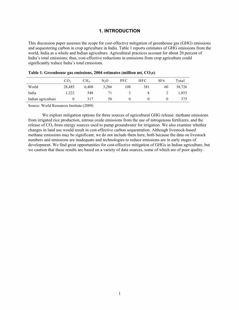
This discussion paper assesses the scope for cost-effective mitigation of greenhouse gas (GHG) emissions and sequestering carbon in crop agriculture in India. Table 1 reports estimates of GHG emissions from the world, India as a whole and Indian agriculture. Agricultural practices account for about 20 percent of India’s total emissions; thus, cost-effective reductions in emissions from crop agriculture could significantly reduce India’s total emissions.

Table 1. Greenhouse gas emissions, 2004 estimates (million mt, CO2e)

CO2 CH4 N2O PFC HFC SF6 Total World 28,485 6,408 3,286 108 381 60 38,726 India 1,222 548 71 3 8 2 1,853 Indian agriculture 0 317 58 0 0 0 375

Source: World Resources Institute (2009)

We explore mitigation options for three sources of agricultural GHG release: methane emissions from irrigated rice production, nitrous oxide emissions from the use of nitrogenous fertilizers, and the release of CO2 from energy sources used to pump groundwater for irrigation. We also examine whether changes in land use would result in cost-effective carbon sequestration. Although livestock-based methane emissions may be significant, we do not include them here, both because the data on livestock numbers and emissions are inadequate and technologies to reduce emissions are in early stages of development. We find great opportunities for cost-effective mitigation of GHGs in Indian agriculture, but we caution that these results are based on a variety of data sources, some of which are of poor quality.

2

2. AGRICULTURE’S ROLE IN GREENHOUSE GAS EMISSIONS AND MITIGATION

Agriculture can play an important role in mitigating three greenhouse gases: carbon dioxide (CO2), methane (CH4), and nitrous oxide (N2O). Plants absorb CO2 from the atmosphere and extract some carbon for use in developing plant tissues. Oxygen (O2) and CO2 are released back into the atmosphere. When the plant dies, the carbon in the plant tissues is converted back to CO2 if decomposition is aerobic, to CH4 if decomposition is anaerobic, or remains in the soil as soil organic material (SOM) if the material does not decompose. Aerobic decomposition takes place where decaying plant material is either on the surface or close to it and exposed to alternating wet and dry periods. Anaerobic decomposition releases CH4 and takes place in fields that are flooded for extended periods, such as those used for paddy rice.

Some agricultural practices remove CO2 from the atmosphere, release oxygen back into the atmosphere, and sequester carbon in the soil for long periods. Any practice that moves plant material down into the soil extends the period that carbon is sequestered. According to researchers at the National Institute for Agricultural Research (INRA), the mean residence time for organic carbon in the soil increases markedly with depth, with rapid turnover (days to months) near the surface and reaching from 2,000 to 10,000 years below 20 cm (INRA 2007).

Changes in land and soil use can trigger changes in soil carbon accumulation. The process is dynamic, involving plant growth above the soil surface and organic carbon accumulation below the surface. Eventually, the system reaches a new soil carbon stock equilibrium or saturation point, and no new carbon is absorbed or lost. This accumulation process can continue for 50 years or longer. Under constant conditions, the amount of soil organic carbon eventually stabilizes, but changes in land management practices can bring soil organic carbon stocks to a new equilibrium, with more or less carbon sequestered than under old practices.

Agricultural practices can also sequester carbon above ground in the form of woody material. This carbon remains sequestered only for as long as the plant remains alive or the products remain in organic form such as lumber or furniture.

N2O release is a byproduct of the plant’s use of nitrogen for growth. Plants extract nitrogen from naturally occurring compounds in the soil, and from organic fertilizers and inorganic nitrogenous fertilizers. Some of the nitrogen contained in fertilizer is not taken up by the plant but is converted to N2O and released to the atmosphere. The nitrogen in either form of fertilizer, inorganic or organic, can be converted to N2O and contribute to global warming.

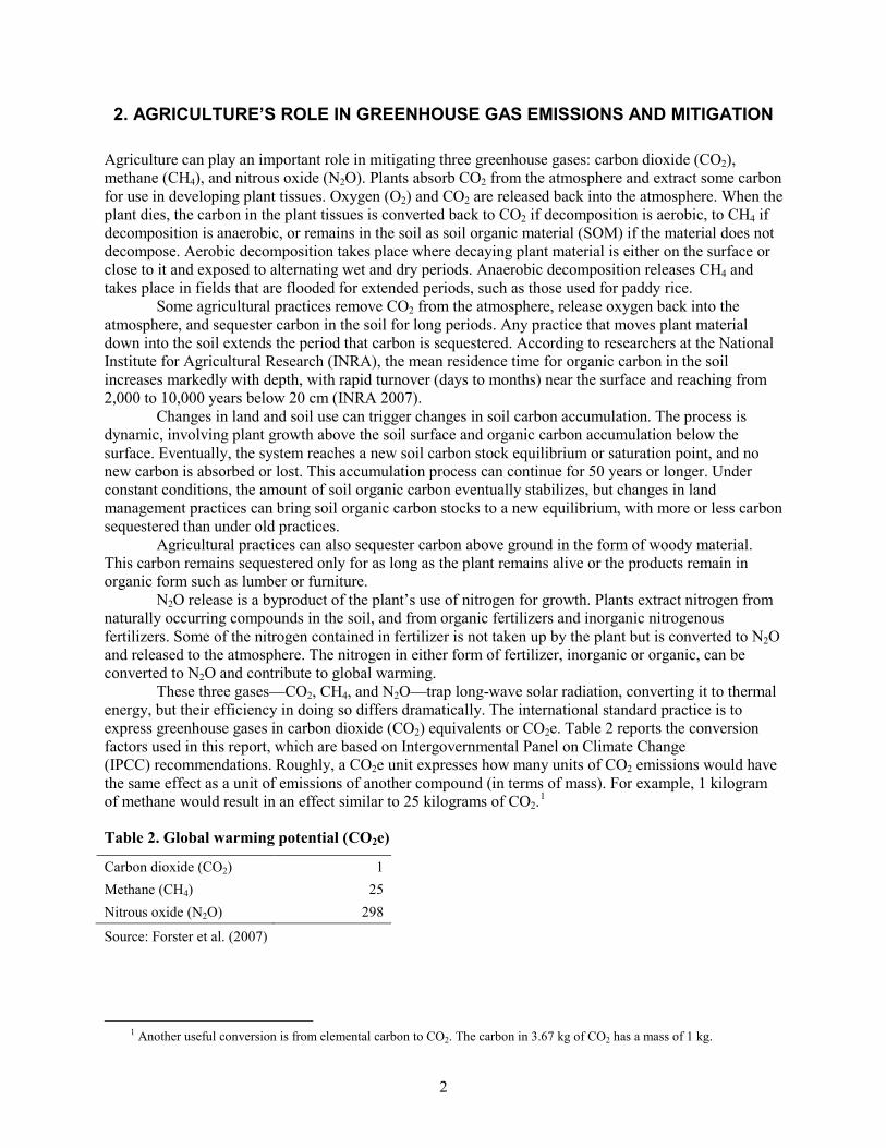
These three gases—CO2, CH4, and N2O—trap long-wave solar radiation, converting it to thermal energy, but their efficiency in doing so differs dramatically. The international standard practice is to express greenhouse gases in carbon dioxide (CO2) equivalents or CO2e. Table 2 reports the conversion factors used in this report, which are based on Intergovernmental Panel on Climate Change (IPCC) recommendations. Roughly, a CO2e unit expresses how many units of CO2 emissions would have the same effect as a unit of emissions of another compound (in terms of mass). For example, 1 kilogram of methane would result in an effect similar to 25 kilograms of CO2.1

Table 2. Global warming potential (CO2e)

Carbon dioxide (CO2) 1 Methane (CH4) 25 Nitrous oxide (N2O) 298

Source: Forster et al. (2007)

1 Another useful conversion is from elemental carbon to CO2. The carbon in 3.67 kg of CO2 has a mass of 1 kg.

3

3. ASSUMPTIONS AND DATA SOURCES

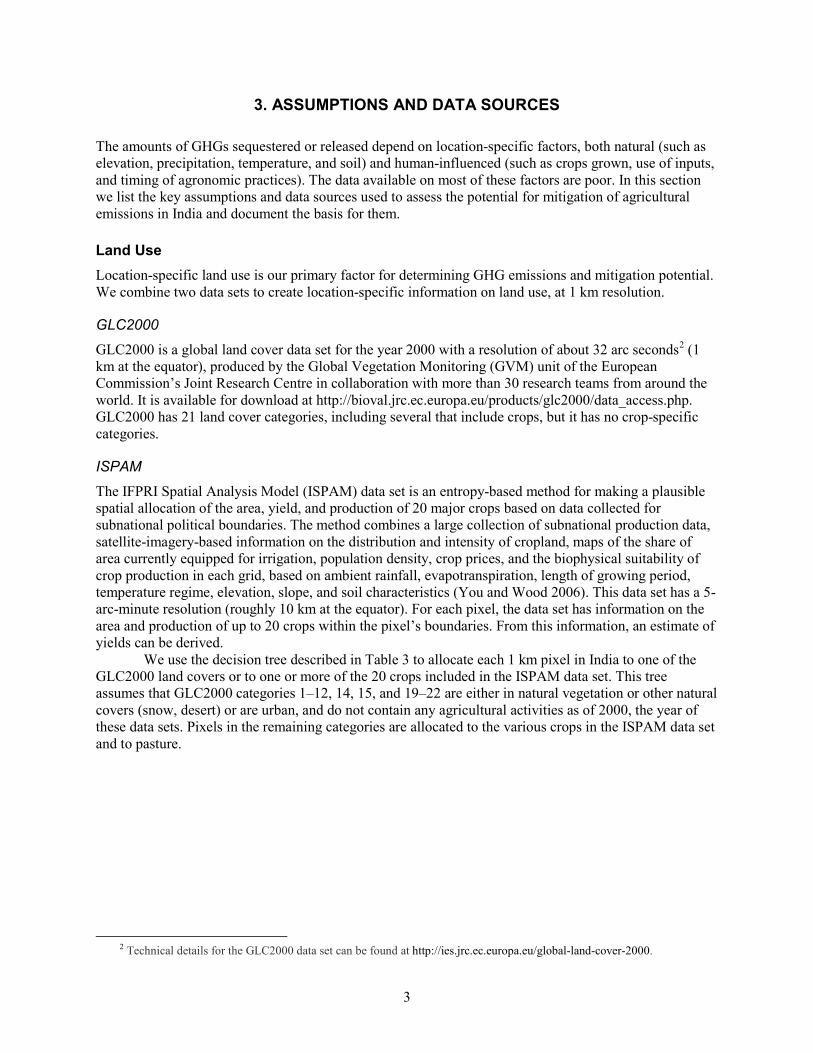
The amounts of GHGs sequestered or released depend on location-specific factors, both natural (such as elevation, precipitation, temperature, and soil) and human-influenced (such as crops grown, use of inputs, and timing of agronomic practices). The data available on most of these factors are poor. In this section we list the key assumptions and data sources used to assess the potential for mitigation of agricultural emissions in India and document the basis for them.

Land Use Location-specific land use is our primary factor for determining GHG emissions and mitigation potential. We combine two data sets to create location-specific information on land use, at 1 km resolution.

GLC2000

GLC2000 is a global land cover data set for the year 2000 with a resolution of about 32 arc seconds2

collaboration

(1 km at the equator), produced by the Global Vegetation Monitoring (GVM) unit of the European Commission’s Joint Research Centre in with more than 30 research teams from around the world. It is available for download at http://bioval.jrc.ec.europa.eu/products/glc2000/data_access.php. GLC2000 has 21 land cover categories, including several that include crops, but it has no crop-specific categories.

ISPAM

The IFPRI Spatial Analysis Model (ISPAM) data set is an entropy-based method for making a plausible spatial allocation of the area, yield, and production of 20 major crops based on data collected for subnational political boundaries. The method combines a large collection of subnational production data, satellite-imagery-based information on the distribution and intensity of cropland, maps of the share of area currently equipped for irrigation, population density, crop prices, and the biophysical suitability of crop production in each grid, based on ambient rainfall, evapotranspiration, length of growing period, temperature regime, elevation, slope, and soil characteristics (You and Wood 2006). This data set has a 5-arc-minute resolution (roughly 10 km at the equator). For each pixel, the data set has information on the area and production of up to 20 crops within the pixel’s boundaries. From this information, an estimate of yields can be derived.

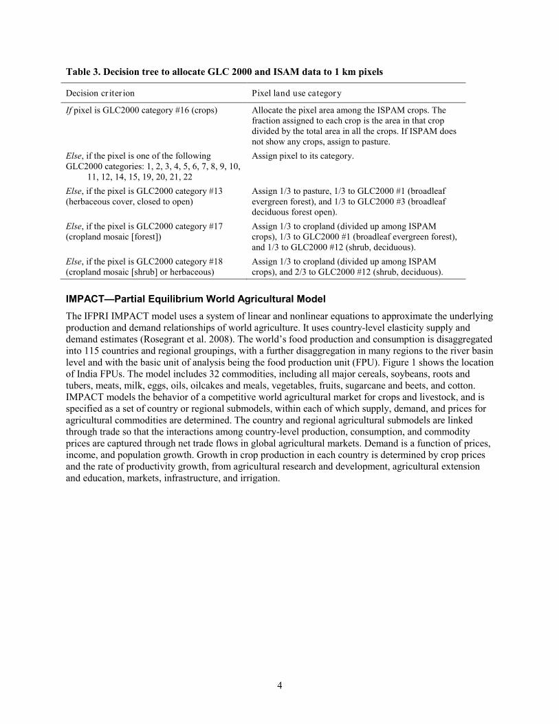
We use the decision tree described in Table 3 to allocate each 1 km pixel in India to one of the GLC2000 land covers or to one or more of the 20 crops included in the ISPAM data set. This tree assumes that GLC2000 categories 1–12, 14, 15, and 19–22 are either in natural vegetation or other natural covers (snow, desert) or are urban, and do not contain any agricultural activities as of 2000, the year of these data sets. Pixels in the remaining categories are allocated to the various crops in the ISPAM data set and to pasture.

2 Technical details for the GLC2000 data set can be found at http://ies.jrc.ec.europa.eu/global-land-cover-2000.

4

Table 3. Decision tree to allocate GLC 2000 and ISAM data to 1 km pixels

Decision cr iter ion Pixel land use category

If pixel is GLC2000 category #16 (crops) Allocate the pixel area among the ISPAM crops. The fraction assigned to each crop is the area in that crop divided by the total area in all the crops. If ISPAM does not show any crops, assign to pasture.

Else, if the pixel is one of the following GLC2000 categories: 1, 2, 3, 4, 5, 6, 7, 8, 9, 10,

11, 12, 14, 15, 19, 20, 21, 22

Assign pixel to its category.

Else, if the pixel is GLC2000 category #13 (herbaceous cover, closed to open)

Assign 1/3 to pasture, 1/3 to GLC2000 #1 (broadleaf evergreen forest), and 1/3 to GLC2000 #3 (broadleaf deciduous forest open).

Else, if the pixel is GLC2000 category #17 (cropland mosaic [forest])

Assign 1/3 to cropland (divided up among ISPAM crops), 1/3 to GLC2000 #1 (broadleaf evergreen forest), and 1/3 to GLC2000 #12 (shrub, deciduous).

Else, if the pixel is GLC2000 category #18 (cropland mosaic [shrub] or herbaceous)

Assign 1/3 to cropland (divided up among ISPAM crops), and 2/3 to GLC2000 #12 (shrub, deciduous).

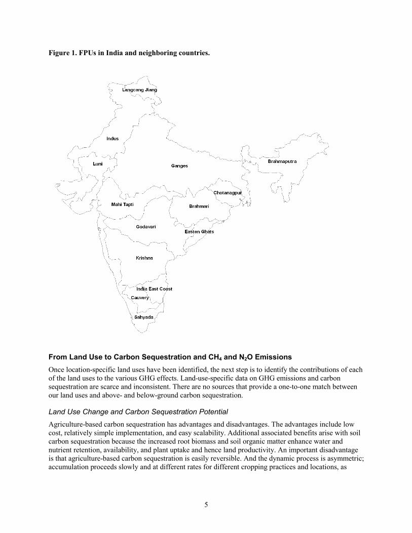
IMPACT—Partial Equilibrium World Agricultural Model The IFPRI IMPACT model uses a system of linear and nonlinear equations to approximate the underlying production and demand relationships of world agriculture. It uses country-level elasticity supply and demand estimates (Rosegrant et al. 2008). The world’s food production and consumption is disaggregated into 115 countries and regional groupings, with a further disaggregation in many regions to the river basin level and with the basic unit of analysis being the food production unit (FPU). Figure 1 shows the location of India FPUs. The model includes 32 commodities, including all major cereals, soybeans, roots and tubers, meats, milk, eggs, oils, oilcakes and meals, vegetables, fruits, sugarcane and beets, and cotton. IMPACT models the behavior of a competitive world agricultural market for crops and livestock, and is specified as a set of country or regional submodels, within each of which supply, demand, and prices for agricultural commodities are determined. The country and regional agricultural submodels are linked through trade so that the interactions among country-level production, consumption, and commodity prices are captured through net trade flows in global agricultural markets. Demand is a function of prices, income, and population growth. Growth in crop production in each country is determined by crop prices and the rate of productivity growth, from agricultural research and development, agricultural extension and education, markets, infrastructure, and irrigation.

5

Figure 1. FPUs in India and neighboring countries.

From Land Use to Carbon Sequestration and CH4 and N2O Emissions Once location-specific land uses have been identified, the next step is to identify the contributions of each of the land uses to the various GHG effects. Land-use-specific data on GHG emissions and carbon sequestration are scarce and inconsistent. There are no sources that provide a one-to-one match between our land uses and above- and below-ground carbon sequestration.

Land Use Change and Carbon Sequestration Potential

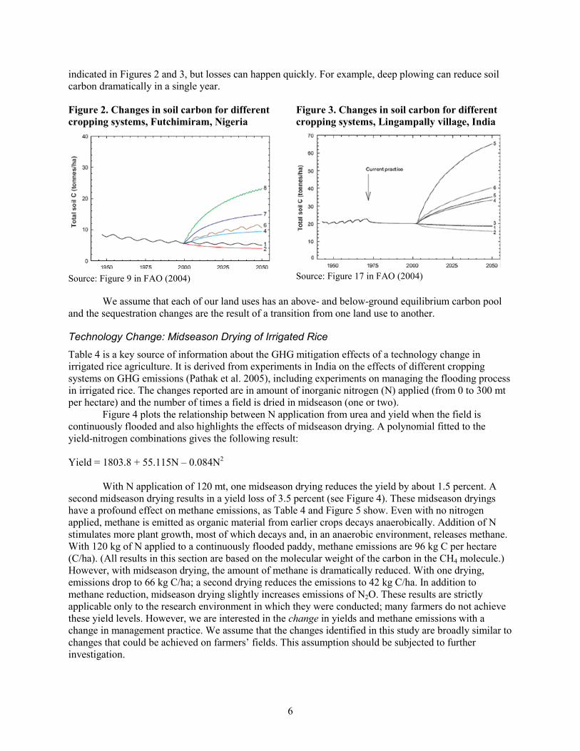
Agriculture-based carbon sequestration has advantages and disadvantages. The advantages include low cost, relatively simple implementation, and easy scalability. Additional associated benefits arise with soil carbon sequestration because the increased root biomass and soil organic matter enhance water and nutrient retention, availability, and plant uptake and hence land productivity. An important disadvantage is that agriculture-based carbon sequestration is easily reversible. And the dynamic process is asymmetric; accumulation proceeds slowly and at different rates for different cropping practices and locations, as

6

indicated in Figures 2 and 3, but losses can happen quickly. For example, deep plowing can reduce soil carbon dramatically in a single year.

Figure 2. Changes in soil carbon for different cropping systems, Futchimiram, Nigeria

Source: Figure 9 in FAO (2004)

Figure 3. Changes in soil carbon for different cropping systems, Lingampally village, India

Source: Figure 17 in FAO (2004)

We assume that each of our land uses has an above- and below-ground equilibrium carbon pool and the sequestration changes are the result of a transition from one land use to another.

Technology Change: Midseason Drying of Irrigated Rice

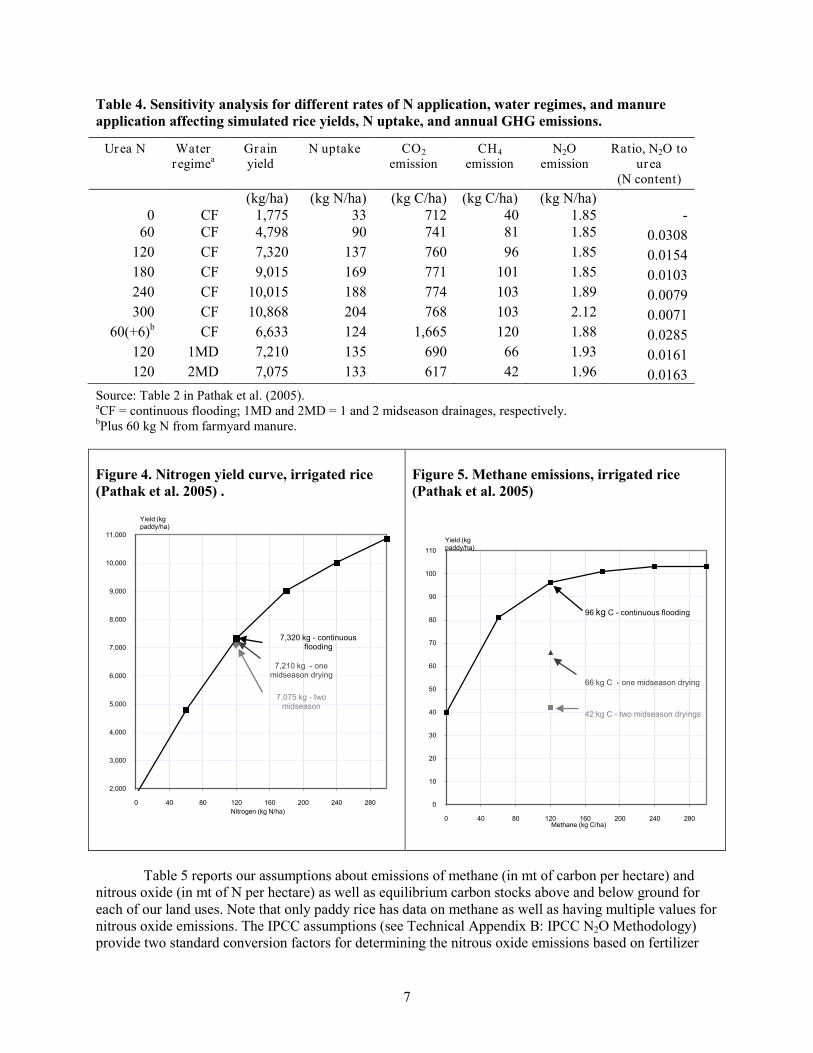
Table 4 is a key source of information about the GHG mitigation effects of a technology change in irrigated rice agriculture. It is derived from experiments in India on the effects of different cropping systems on GHG emissions (Pathak et al. 2005), including experiments on managing the flooding process in irrigated rice. The changes reported are in amount of inorganic nitrogen (N) applied (from 0 to 300 mt per hectare) and the number of times a field is dried in midseason (one or two).

Figure 4 plots the relationship between N application from urea and yield when the field is continuously flooded and also highlights the effects of midseason drying. A polynomial fitted to the yield-nitrogen combinations gives the following result: Yield = 1803.8 + 55.115N – 0.084N2

With N application of 120 mt, one midseason drying reduces the yield by about 1.5 percent. A

second midseason drying results in a yield loss of 3.5 percent (see Figure 4). These midseason dryings have a profound effect on methane emissions, as Table 4 and Figure 5 show. Even with no nitrogen applied, methane is emitted as organic material from earlier crops decays anaerobically. Addition of N stimulates more plant growth, most of which decays and, in an anaerobic environment, releases methane. With 120 kg of N applied to a continuously flooded paddy, methane emissions are 96 kg C per hectare (C/ha). (All results in this section are based on the molecular weight of the carbon in the CH4 molecule.) However, with midseason drying, the amount of methane is dramatically reduced. With one drying, emissions drop to 66 kg C/ha; a second drying reduces the emissions to 42 kg C/ha. In addition to methane reduction, midseason drying slightly increases emissions of N2O. These results are strictly applicable only to the research environment in which they were conducted; many farmers do not achieve these yield levels. However, we are interested in the change in yields and methane emissions with a change in management practice. We assume that the changes identified in this study are broadly similar to changes that could be achieved on farmers’ fields. This assumption should be subjected to further investigation.

7

Table 4. Sensitivity analysis for different rates of N application, water regimes, and manure application affecting simulated rice yields, N uptake, and annual GHG emissions.

Urea N Water regimea

Grain yield

N uptake CO2 emission

CH4 emission

N2O emission

Ratio, N2O to urea

(N content) (kg/ha) (kg N/ha) (kg C/ha) (kg C/ha) (kg N/ha)

0 CF 1,775 33 712 40 1.85 - 60 CF 4,798 90 741 81 1.85 0.0308

120 CF 7,320 137 760 96 1.85 0.0154 180 CF 9,015 169 771 101 1.85 0.0103 240 CF 10,015 188 774 103 1.89 0.0079 300 CF 10,868 204 768 103 2.12 0.0071

60(+6)b CF 6,633 124 1,665 120 1.88 0.0285 120 1MD 7,210 135 690 66 1.93 0.0161 120 2MD 7,075 133 617 42 1.96 0.0163

Source: Table 2 in Pathak et al. (2005). aCF = continuous flooding; 1MD and 2MD = 1 and 2 midseason drainages, respectively. bPlus 60 kg N from farmyard manure.

Figure 4. Nitrogen yield curve, irrigated rice (Pathak et al. 2005) .

Figure 5. Methane emissions, irrigated rice (Pathak et al. 2005)

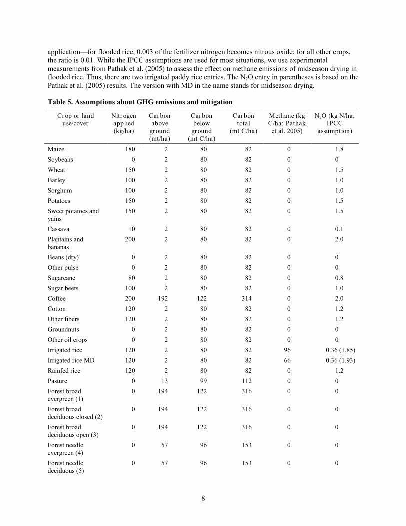
Table 5 reports our assumptions about emissions of methane (in mt of carbon per hectare) and nitrous oxide (in mt of N per hectare) as well as equilibrium carbon stocks above and below ground for each of our land uses. Note that only paddy rice has data on methane as well as having multiple values for nitrous oxide emissions. The IPCC assumptions (see Technical Appendix B: IPCC N2O Methodology) provide two standard conversion factors for determining the nitrous oxide emissions based on fertilizer

2,000

3,000

4,000

5,000

6,000

7,000

8,000

9,000

10,000

11,000

0 40 80 120 160 200 240 280

Yield (kg paddy/ha)

Nitrogen (kg N/ha)

7,320 kg - continuous flooding

7,210 kg - one midseason drying

7,075 kg - two midseason

0

10

20

30

40

50

60

70

80

90

100

110

0 40 80 120 160 200 240 280

Yield (kg paddy/ha)

Methane (kg C/ha)

96 kg C - continuous flooding

66 kg C - one midseason drying

42 kg C - two midseason dryings

8

application—for flooded rice, 0.003 of the fertilizer nitrogen becomes nitrous oxide; for all other crops, the ratio is 0.01. While the IPCC assumptions are used for most situations, we use experimental measurements from Pathak et al. (2005) to assess the effect on methane emissions of midseason drying in flooded rice. Thus, there are two irrigated paddy rice entries. The N2O entry in parentheses is based on the Pathak et al. (2005) results. The version with MD in the name stands for midseason drying.

Table 5. Assumptions about GHG emissions and mitigation

Crop or land use/cover

Nitrogen applied (kg/ha)

Carbon above

ground (mt/ha)

Carbon below

ground (mt C/ha)

Carbon total

(mt C/ha)

Methane (kg C/ha; Pathak

et al. 2005)

N2O (kg N/ha; IPCC

assumption)

Maize 180 2 80 82 0 1.8 Soybeans 0 2 80 82 0 0 Wheat 150 2 80 82 0 1.5 Barley 100 2 80 82 0 1.0 Sorghum 100 2 80 82 0 1.0 Potatoes 150 2 80 82 0 1.5 Sweet potatoes and yams

150 2 80 82 0 1.5

Cassava 10 2 80 82 0 0.1 Plantains and bananas

200 2 80 82 0 2.0

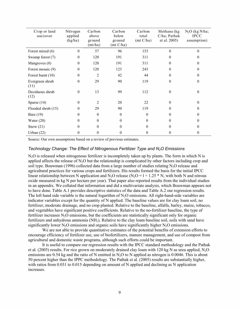
Beans (dry) 0 2 80 82 0 0 Other pulse 0 2 80 82 0 0 Sugarcane 80 2 80 82 0 0.8 Sugar beets 100 2 80 82 0 1.0 Coffee 200 192 122 314 0 2.0 Cotton 120 2 80 82 0 1.2 Other fibers 120 2 80 82 0 1.2 Groundnuts 0 2 80 82 0 0 Other oil crops 0 2 80 82 0 0 Irrigated rice 120 2 80 82 96 0.36 (1.85) Irrigated rice MD 120 2 80 82 66 0.36 (1.93) Rainfed rice 120 2 80 82 0 1.2 Pasture 0 13 99 112 0 0 Forest broad evergreen (1)

0 194 122 316 0 0

Forest broad deciduous closed (2)

0 194 122 316 0 0

Forest broad deciduous open (3)

0 194 122 316 0 0

Forest needle evergreen (4)

0 57 96 153 0 0

Forest needle deciduous (5)

0 57 96 153 0 0

9

Crop or land use/cover

Nitrogen applied (kg/ha)

Carbon above

ground (mt/ha)

Carbon below

ground (mt C/ha)

Carbon total

(mt C/ha)

Methane (kg C/ha; Pathak

et al. 2005)

N2O (kg N/ha; IPCC

assumption)

Forest mixed (6) 0 57 96 153 0 0 Swamp forest (7) 0 120 191 311 0 0 Mangroves (8) 0 120 191 311 0 0 Forest mosaic (9) 0 120 123 243 0 0 Forest burnt (10) 0 2 42 44 0 0 Evergreen shrub (11)

0 29 90 119 0 0

Deciduous shrub (12)

0 13 99 112 0 0

Sparse (14) 0 2 20 22 0 0 Flooded shrub (15) 0 29 90 119 0 0 Bare (19) 0 0 0 0 0 0 Water (20) 0 0 0 0 0 0 Snow (21) 0 0 0 0 0 0 Urban (22) 0 0 0 0 0 0

Source: Our own assumptions based on a review of previous estimates.

Technology Change: The Effect of Nitrogenous Fertilizer Type and N2O Emissions

N2O is released when nitrogenous fertilizer is incompletely taken up by plants. The form in which N is applied affects the release of N2O but the relationship is complicated by other factors including crop and soil type. Bouwman (1996) collected data from a large number of studies relating N2O release and agricultural practices for various crops and fertilizers. His results formed the basis for the initial IPCC linear relationship between N application and N2O release (N2O = l + 1.25 * N, with both N and nitrous oxide measured in kg N per hectare per year). That paper also reported results from the individual studies in an appendix. We collated that information and did a multivariate analysis, which Bouwman appears not to have done. Table A.1 provides descriptive statistics of the data and Table A.2 our regression results. The left hand side variable is the natural logarithm of N2O emissions. All right-hand-side variables are indicator variables except for the quantity of N applied. The baseline values are for clay loam soil, no fertilizer, moderate drainage, and no crop planted. Relative to the baseline, alfalfa, barley, maize, tobacco, and vegetables have significant positive coefficients. Relative to the no-fertilizer baseline, the type of fertilizer increases N2O emissions, but the coefficients are statistically significant only for organic fertilizers and anhydrous ammonia (NH3). Relative to the clay loam baseline soil, soils with sand have significantly lower N2O emissions and organic soils have significantly higher N2O emissions.

We are not able to provide quantitative estimates of the potential benefits of extension efforts to encourage efficiency of fertilizer use, use of biofertilizers, manure management, and use of compost from agricultural and domestic waste programs, although such efforts could be important.

It is useful to compare our regression results with the IPCC standard methodology and the Pathak et al. (2005) results. For rice grown on moderately drained clay loam with 120 kg N as urea applied, N2O emissions are 0.54 kg and the ratio of N emitted in N2O to N applied as nitrogen is 0.0046. This is about 50 percent higher than the IPPC methodology. The Pathak et al. (2005) results are substantially higher, with ratios from 0.031 to 0.015 depending on amount of N applied and declining as N application increases.

10

Carbon Pool and GHG Emissions Estimates

Carbon Pool

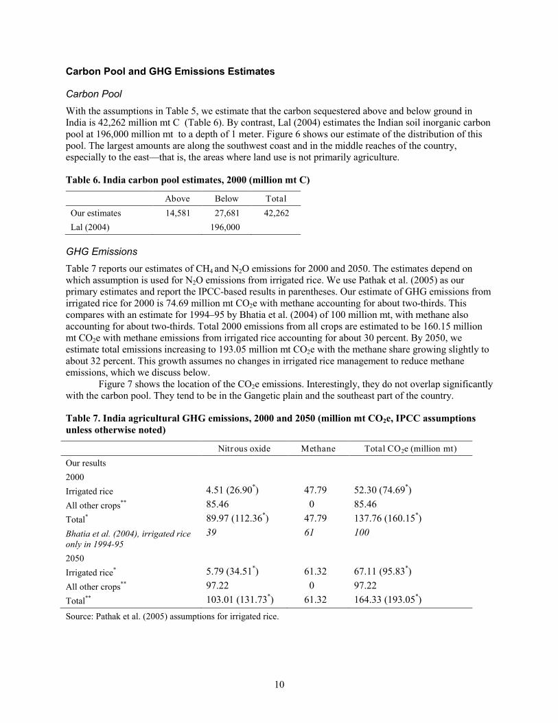
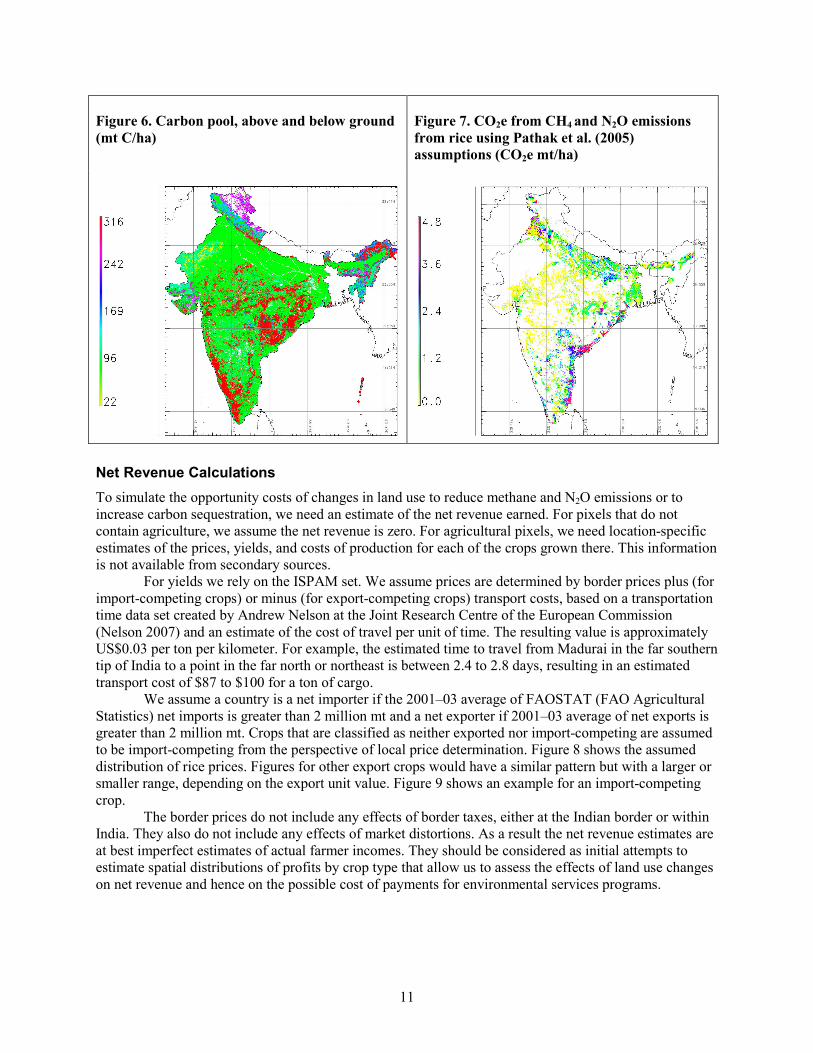
With the assumptions in Table 5, we estimate that the carbon sequestered above and below ground in India is 42,262 million mt C (Table 6). By contrast, Lal (2004) estimates the Indian soil inorganic carbon pool at 196,000 million mt to a depth of 1 meter. Figure 6 shows our estimate of the distribution of this pool. The largest amounts are along the southwest coast and in the middle reaches of the country, especially to the east—that is, the areas where land use is not primarily agriculture.

Table 6. India carbon pool estimates, 2000 (million mt C)

Above Below Total Our estimates 14,581 27,681 42,262 Lal (2004) 196,000

GHG Emissions

Table 7 reports our estimates of CH4 and N2O emissions for 2000 and 2050. The estimates depend on which assumption is used for N2O emissions from irrigated rice. We use Pathak et al. (2005) as our primary estimates and report the IPCC-based results in parentheses. Our estimate of GHG emissions from irrigated rice for 2000 is 74.69 million mt CO2e with methane accounting for about two-thirds. This compares with an estimate for 1994–95 by Bhatia et al. (2004) of 100 million mt, with methane also accounting for about two-thirds. Total 2000 emissions from all crops are estimated to be 160.15 million mt CO2e with methane emissions from irrigated rice accounting for about 30 percent. By 2050, we estimate total emissions increasing to 193.05 million mt CO2e with the methane share growing slightly to about 32 percent. This growth assumes no changes in irrigated rice management to reduce methane emissions, which we discuss below.

Figure 7 shows the location of the CO2e emissions. Interestingly, they do not overlap significantly with the carbon pool. They tend to be in the Gangetic plain and the southeast part of the country.

Table 7. India agricultural GHG emissions, 2000 and 2050 (million mt CO2e, IPCC assumptions unless otherwise noted)

Nitrous oxide Methane Total CO2e (million mt) Our results 2000 Irrigated rice 4.51 (26.90*) 47.79 52.30 (74.69*) All other crops** 85.46 0 85.46 Total* 89.97 (112.36*) 47.79 137.76 (160.15*) Bhatia et al. (2004), irrigated rice only in 1994-95

39 61 100

2050 Irrigated rice* 5.79 (34.51*) 61.32 67.11 (95.83*) All other crops** 97.22 0 97.22 Total** 103.01 (131.73*) 61.32 164.33 (193.05*) Source: Pathak et al. (2005) assumptions for irrigated rice.

11

Figure 6. Carbon pool, above and below ground (mt C/ha)

Figure 7. CO2e from CH4 and N2O emissions from rice using Pathak et al. (2005) assumptions (CO2e mt/ha)

Net Revenue Calculations To simulate the opportunity costs of changes in land use to reduce methane and N2O emissions or to increase carbon sequestration, we need an estimate of the net revenue earned. For pixels that do not contain agriculture, we assume the net revenue is zero. For agricultural pixels, we need location-specific estimates of the prices, yields, and costs of production for each of the crops grown there. This information is not available from secondary sources.

For yields we rely on the ISPAM set. We assume prices are determined by border prices plus (for import-competing crops) or minus (for export-competing crops) transport costs, based on a transportation time data set created by Andrew Nelson at the Joint Research Centre of the European Commission (Nelson 2007) and an estimate of the cost of travel per unit of time. The resulting value is approximately US$0.03 per ton per kilometer. For example, the estimated time to travel from Madurai in the far southern tip of India to a point in the far north or northeast is between 2.4 to 2.8 days, resulting in an estimated transport cost of $87 to $100 for a ton of cargo.

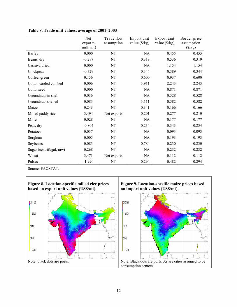
We assume a country is a net importer if the 2001–03 average of FAOSTAT (FAO Agricultural Statistics) net imports is greater than 2 million mt and a net exporter if 2001–03 average of net exports is greater than 2 million mt. Crops that are classified as neither exported nor import-competing are assumed to be import-competing from the perspective of local price determination. Figure 8 shows the assumed distribution of rice prices. Figures for other export crops would have a similar pattern but with a larger or smaller range, depending on the export unit value. Figure 9 shows an example for an import-competing crop.

The border prices do not include any effects of border taxes, either at the Indian border or within India. They also do not include any effects of market distortions. As a result the net revenue estimates are at best imperfect estimates of actual farmer incomes. They should be considered as initial attempts to estimate spatial distributions of profits by crop type that allow us to assess the effects of land use changes on net revenue and hence on the possible cost of payments for environmental services programs.

12

Table 8. Trade unit values, average of 2001–2003

Net expor ts

(mill. mt)

Trade flow assumption

Impor t unit value ($/kg)

Expor t unit value ($/kg)

Border pr ice assumption

($/kg) Barley 0.000 NT NA 0.455 0.455 Beans, dry -0.297 NT 0.319 0.536 0.319 Cassava dried 0.000 NT NA 1.154 1.154 Chickpeas -0.329 NT 0.344 0.389 0.344 Coffee, green 0.156 NT 0.600 0.937 0.600 Cotton carded combed 0.006 NT 3.911 2.243 2.243 Cottonseed 0.000 NT NA 0.871 0.871 Groundnuts in shell 0.036 NT NA 0.528 0.528 Groundnuts shelled 0.083 NT 3.111 0.582 0.582 Maize 0.243 NT 0.341 0.166 0.166 Milled paddy rice 3.494 Net exports 0.201 0.277 0.210 Millet 0.028 NT NA 0.177 0.177 Peas, dry -0.804 NT 0.234 0.343 0.234 Potatoes 0.037 NT NA 0.093 0.093 Sorghum 0.005 NT NA 0.193 0.193 Soybeans 0.083 NT 0.784 0.230 0.230 Sugar (centrifugal, raw) 0.268 NT NA 0.232 0.232 Wheat 3.471 Net exports NA 0.112 0.112 Pulses -1.990 NT 0.294 0.482 0.294

Source: FAOSTAT.

Figure 8. Location-specific milled rice prices based on export unit values (US$/mt).

Figure 9. Location-specific maize prices based on import unit values (US$/mt).

Note: black dots are ports.

Note: Black dots are ports. Xs are cities assumed to be consumption centers.

13

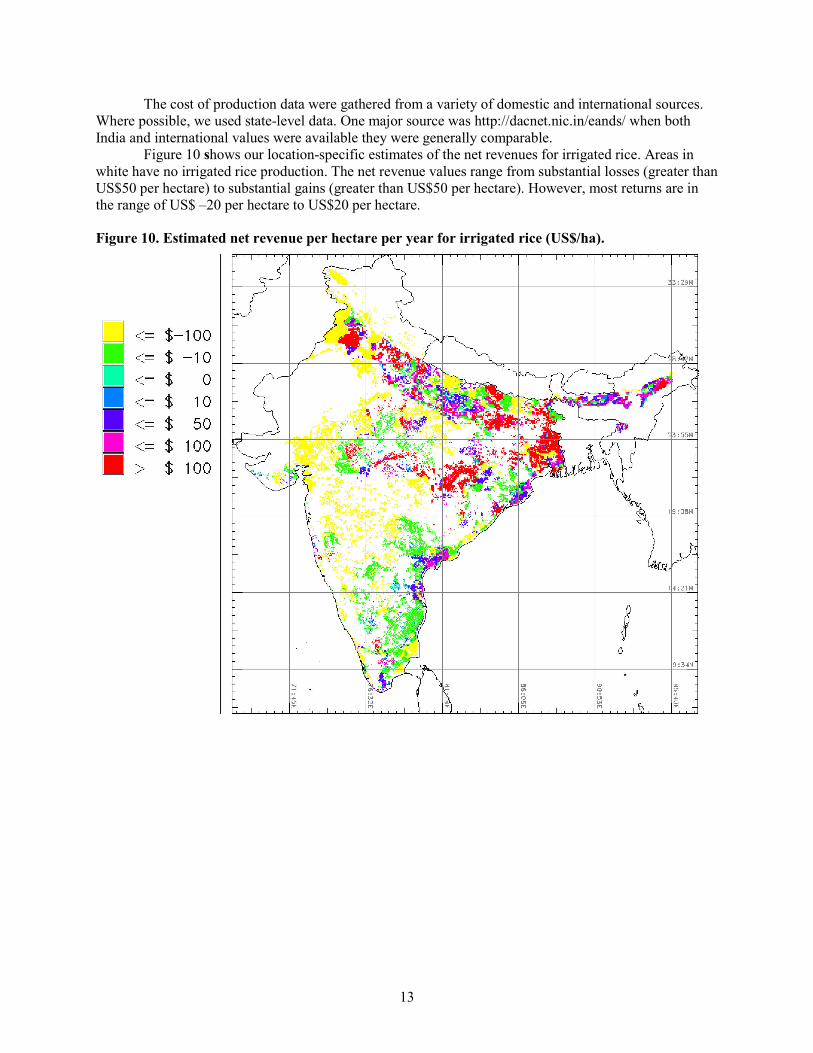
The cost of production data were gathered from a variety of domestic and international sources. Where possible, we used state-level data. One major source was http://dacnet.nic.in/eands/ when both India and international values were available they were generally comparable.

Figure 10 shows our location-specific estimates of the net revenues for irrigated rice. Areas in white have no irrigated rice production. The net revenue values range from substantial losses (greater than US$50 per hectare) to substantial gains (greater than US$50 per hectare). However, most returns are in the range of US$ –20 per hectare to US$20 per hectare.

Figure 10. Estimated net revenue per hectare per year for irrigated rice (US$/ha).

14

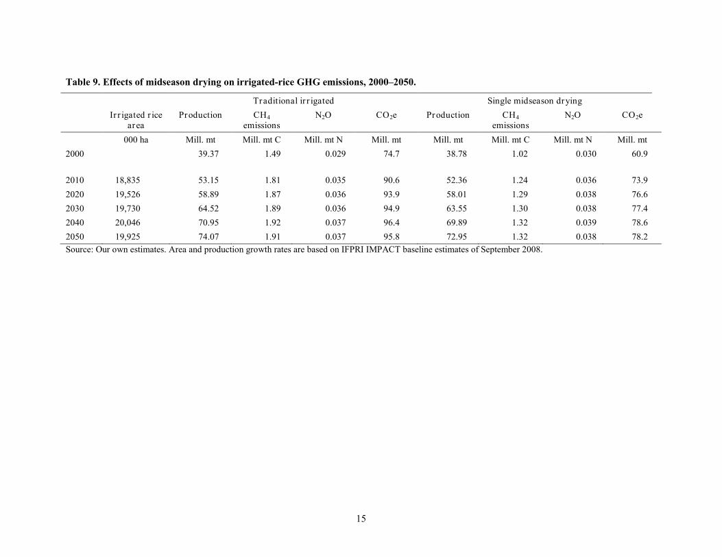
4. EFFECTS OF MIDSEASON DRYING ON METHANE EMISSIONS

In this section, we report the results of a complete conversion of irrigated rice from continuous flooding to a single midseason drying. Table 9 provides summary statistics. The results are based on projections for rice agriculture from the IMPACT model along with the emission rates reported in Pathak et al. (2005). The combined emissions of methane and N2O in irrigated rice agriculture in 2000 result in 75.7 million mt CO2e. If all of this area used a single midseason drying, CO2e drops to 60.9 million mt, a decline of about 20 percent.

The growth in emissions in the out-years to 2050 is based on the growth rates in irrigated area predicted by the IMPACT model. Without a technology change, CO2e rises about 28 percent by 2050. With complete adoption of the drying technology, the CO2e in 2050 is less than 5 percent higher than the CO2e emissions in 2000 and lower than the projections for 2010, even with the increase in area and accompanying nitrogen application.

15

Table 9. Effects of midseason drying on irrigated-rice GHG emissions, 2000–2050.

Traditional ir r igated Single midseason drying Ir r igated r ice

area Production CH4

emissions N2O CO2e Production CH4

emissions N2O CO2e

000 ha Mill. mt Mill. mt C Mill. mt N Mill. mt Mill. mt Mill. mt C Mill. mt N Mill. mt 2000

39.37 1.49 0.029 74.7 38.78 1.02 0.030 60.9

2010 18,835 53.15 1.81 0.035 90.6 52.36 1.24 0.036 73.9 2020 19,526 58.89 1.87 0.036 93.9 58.01 1.29 0.038 76.6 2030 19,730 64.52 1.89 0.036 94.9 63.55 1.30 0.038 77.4 2040 20,046 70.95 1.92 0.037 96.4 69.89 1.32 0.039 78.6 2050 19,925 74.07 1.91 0.037 95.8 72.95 1.32 0.038 78.2 Source: Our own estimates. Area and production growth rates are based on IFPRI IMPACT baseline estimates of September 2008.

16

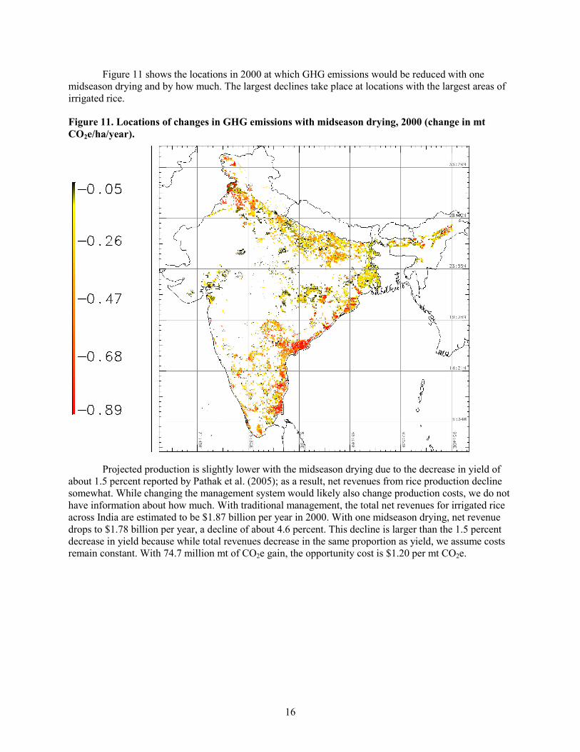
Figure 11 shows the locations in 2000 at which GHG emissions would be reduced with one midseason drying and by how much. The largest declines take place at locations with the largest areas of irrigated rice.

Figure 11. Locations of changes in GHG emissions with midseason drying, 2000 (change in mt CO2e/ha/year).

Projected production is slightly lower with the midseason drying due to the decrease in yield of about 1.5 percent reported by Pathak et al. (2005); as a result, net revenues from rice production decline somewhat. While changing the management system would likely also change production costs, we do not have information about how much. With traditional management, the total net revenues for irrigated rice across India are estimated to be $1.87 billion per year in 2000. With one midseason drying, net revenue drops to $1.78 billion per year, a decline of about 4.6 percent. This decline is larger than the 1.5 percent decrease in yield because while total revenues decrease in the same proportion as yield, we assume costs remain constant. With 74.7 million mt of CO2e gain, the opportunity cost is $1.20 per mt CO2e.

17

5. EFFECTS OF FERTILIZER TYPE ON N2O EMISSIONS

Since the regression results do not find any significant effect of fertilizer type on N2O emissions for the types available in India, we assume these effects are zero. We are not able to provide quantitative estimates of the potential benefits of extension efforts to encourage efficiency of fertilizer use, use of biofertilizers, manure management, and use of compost from agricultural and domestic waste programs, although such efforts could be important.

18

6. EMISSIONS OF CO2 FROM GROUNDWATER PUMPING3

Groundwater lifting requires energy. That energy can come from humans (using treadle pumps), animals, hydro, nuclear power, and fossil fuels. Only fossil fuels contribute significantly to CO2 emissions, and they are by far the most important energy sources for groundwater pumping. Two different fossil fuels provide pumping energy: diesel and coal. Diesel fuel is transported close to the well location and used to power a diesel pump. Electric pumps rely on electricity produced mostly from coal although hydro power accounts for about 13 percent and nuclear 3 percent of total Indian electricity output (source: Table 3.1 in Central Electricity Authority [2005]). This electricity is transported, sometimes long distances, to electric pumps near the fields to be irrigated.

With a 100 percent efficient process, the energy needed to lift 1,000 m3 of water 1 meter is 9.8 * 106 joules (equal to 2.724 kWh). CO2 emissions depend on the efficiency of the power transmission and pumping process and the carbon density of the energy source. In India, the carbon emissions from coal-fired electricity are almost six times greater than from diesel. In our baseline assumptions, we use conservative estimates of 5 percent electricity transmission loss and 30 percent efficiency for both diesel and electric pumps. Once the water is at the surface, further losses occur in transmission and evaporation.

The amount of irrigation water needed by a crop depends on the physiology of the plant and the climate conditions where it is grown. The IMPACT model includes values for each crop in each of the FPUs in India. It also assumes increases in efficiency over time.

The use of groundwater in Indian irrigation has grown rapidly as has the role of deep wells. Between 1950 and 2000, canal-based irrigation increased 8.3 million hectares to 18 million hectares (slightly more than doubling), while groundwater-based irrigation increased more than five-fold, from 6 million hectares to 33.6 million hectares (Ministry of Agriculture). Wells are being excavated deeper, and powered by electric motors as subsidized electricity has made it more cost-effective for farmers to invest in electric pumps instead of diesel pumps. In our forward-looking scenarios we assume all growth in water consumption comes from deep electric wells.

To summarize our baseline assumptions: • Deep wells lift water 75 meters; shallow wells lift water 15 meters. • The energy needed to lift 1,000 m3 of water a distance of 1 meter is 2.724 kWh with no

efficiency losses. • The efficiency of both electric and diesel pumps is 30 percent in terms of theoretical

energy needed to lift water divided by actual energy used. • Electricity transmission losses are 5 percent of the total. • The carbon density of diesel fuel is 0.0732 kg C per kWh; the carbon density of

electricity is 0.4062 kg C per kWh. • The carbon emissions to lift a 1,000 m3 of water 1 meter are 0.665 kg C with diesel-

fueled pumps and 3.873 kg C with electric pumps.

These set of assumptions likely underestimate the contribution of electricity use to CO2 emissions. For example, the transmission electricity losses are believed by some observers to be on the order of 25 percent. The efficiency losses in pumps are likely to make the conversion from actual to theoretical pump efficiency 20 percent or lower.

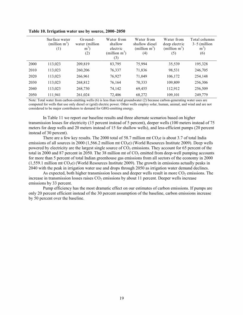
Table 10 reports IMPACT model water results in columns 1 and 2 and our allocations of groundwater to shallow electric and diesel wells and deep electric wells based on district-level counts of wells by type. Our assumption about the future growth of water use coming from deep wells results in a three-fold increase in use of water from that source between 2000 and 2050. Interestingly, the growth stops by 2040 as increasing efficiency of water use offsets demand from more agricultural production.

3 The technical details behind these calculations are reported in Technical Appendix D.

19

Table 10. Irrigation water use by source, 2000–2050

Sur face water (million m3)

(1)

Ground- water (million

m3) (2)

Water from shallow electr ic

(million m3) (3)

Water from shallow diesel (million m3)

(4)

Water from deep electr ic (million m3)

(5)

Total columns 3–5 (million

m3) (6)

2000 113,023 209,819 83,795 75,994 35,539 195,328 2010 113,023 260,206 76,337 71,836 98,531 246,705 2020 113,023 266,961 76,927 71,049 106,172 254,148 2030 113,023 268,812 76,164 70,333 109,809 256,306 2040 113,023 268,730 74,142 69,455 112,912 256,509 2050 111,941 261,024 72,406 68,272 109,101 249,779 Note: Total water from carbon-emitting wells (6) is less than total groundwater (2) because carbon-generating water uses are computed for wells that use only diesel or (grid) electric power. Other wells employ solar, human, animal, and wind and are not considered to be major contributors to demand for GHG-emitting energy.

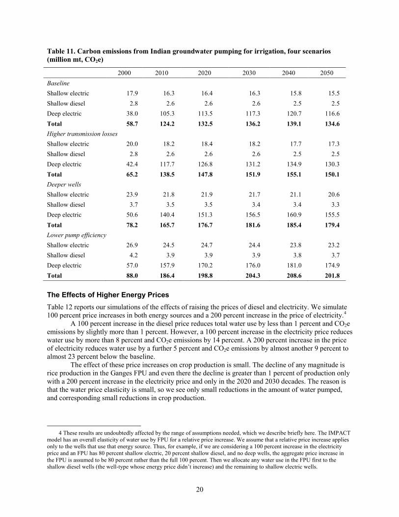
In Table 11 we report our baseline results and three alternate scenarios based on higher transmission losses for electricity (15 percent instead of 5 percent), deeper wells (100 meters instead of 75 meters for deep wells and 20 meters instead of 15 for shallow wells), and less-efficient pumps (20 percent instead of 30 percent).

There are a few key results. The 2000 total of 58.7 million mt CO2e is about 3.7 of total India emissions of all sources in 2000 (1,566.2 million mt CO2e) (World Resources Institute 2009). Deep wells powered by electricity are the largest single source of CO2 emissions. They account for 65 percent of the total in 2000 and 87 percent in 2050. The 38 million mt of CO2 emitted from deep-well pumping accounts for more than 5 percent of total Indian greenhouse gas emissions from all sectors of the economy in 2000 (1,559.1 million mt CO2e) (World Resources Institute 2009). The growth in emissions actually peaks in 2040 with the peak in irrigation water use and drops through 2050 as irrigation water demand declines.

As expected, both higher transmission losses and deeper wells result in more CO2 emissions. The increase in transmission losses raises CO2 emissions by about 11 percent. Deeper wells increase emissions by 33 percent.

Pump efficiency has the most dramatic effect on our estimates of carbon emissions. If pumps are only 20 percent efficient instead of the 30 percent assumption of the baseline, carbon emissions increase by 50 percent over the baseline.

20

Table 11. Carbon emissions from Indian groundwater pumping for irrigation, four scenarios (million mt, CO2e)

2000 2010 2020 2030 2040 2050 Baseline Shallow electric 17.9 16.3 16.4 16.3 15.8 15.5 Shallow diesel 2.8 2.6 2.6 2.6 2.5 2.5 Deep electric 38.0 105.3 113.5 117.3 120.7 116.6 Total 58.7 124.2 132.5 136.2 139.1 134.6 Higher transmission losses Shallow electric 20.0 18.2 18.4 18.2 17.7 17.3 Shallow diesel 2.8 2.6 2.6 2.6 2.5 2.5 Deep electric 42.4 117.7 126.8 131.2 134.9 130.3 Total 65.2 138.5 147.8 151.9 155.1 150.1 Deeper wells Shallow electric 23.9 21.8 21.9 21.7 21.1 20.6 Shallow diesel 3.7 3.5 3.5 3.4 3.4 3.3 Deep electric 50.6 140.4 151.3 156.5 160.9 155.5 Total 78.2 165.7 176.7 181.6 185.4 179.4 Lower pump efficiency Shallow electric 26.9 24.5 24.7 24.4 23.8 23.2 Shallow diesel 4.2 3.9 3.9 3.9 3.8 3.7 Deep electric 57.0 157.9 170.2 176.0 181.0 174.9 Total 88.0 186.4 198.8 204.3 208.6 201.8

The Effects of Higher Energy Prices Table 12 reports our simulations of the effects of raising the prices of diesel and electricity. We simulate 100 percent price increases in both energy sources and a 200 percent increase in the price of electricity.4

A 100 percent increase in the diesel price reduces total water use by less than 1 percent and CO2e emissions by slightly more than 1 percent. However, a 100 percent increase in the electricity price reduces water use by more than 8 percent and CO2e emissions by 14 percent. A 200 percent increase in the price of electricity reduces water use by a further 5 percent and CO2e emissions by almost another 9 percent to almost 23 percent below the baseline.

The effect of these price increases on crop production is small. The decline of any magnitude is rice production in the Ganges FPU and even there the decline is greater than 1 percent of production only with a 200 percent increase in the electricity price and only in the 2020 and 2030 decades. The reason is that the water price elasticity is small, so we see only small reductions in the amount of water pumped, and corresponding small reductions in crop production.

4 These results are undoubtedly affected by the range of assumptions needed, which we describe briefly here. The IMPACT

model has an overall elasticity of water use by FPU for a relative price increase. We assume that a relative price increase applies only to the wells that use that energy source. Thus, for example, if we are considering a 100 percent increase in the electricity price and an FPU has 80 percent shallow electric, 20 percent shallow diesel, and no deep wells, the aggregate price increase in the FPU is assumed to be 80 percent rather than the full 100 percent. Then we allocate any water use in the FPU first to the shallow diesel wells (the well-type whose energy price didn’t increase) and the remaining to shallow electric wells.

21

Table 12. The effects on groundwater pumping of energy price increases.

100 percent increase in diesel pr ice

100 percent increase in electr icity pr ice

200 percent increase in electr icity pr ice

Change in total water

use (percent)

Change in CO2e, (percent)

Change in total water use

(percent)

Change in CO2e, (percent)

Change in total water use (percent)

Change in CO2e,

(percent)

2010 -0.77 -1.11 -8.16 -14.00 -13.36 -22.92

2020 -0.78 -1.08 -8.18 -13.75 -13.34 -22.45

2030 -0.74 -1.06 -8.12 -13.49 -13.31 -22.10

2040 -0.73 -1.03 -8.11 -13.30 -13.24 -21.69

2050 -0.73 -1.05 -8.10 -13.44 -13.24 -21.94

22

7. CARBON SEQUESTRATION SUPPLY CURVES AND EFFICIENCY OF PAYMENT SCHEMES

The goal of this section is to develop a conceptual approach, and implement it empirically, to identify locations where land use change would provide the most carbon sequestered per unit of payment. We compare two payment instruments: a payment per unit of carbon sequestered and a foregone-revenues or opportunity-cost-based payment.

Conceptual Approach We assume that farmers are willing to change to a land use with higher environmental benefits only if they receive a payment at least equal to the loss in net revenue from the change. Since funds are limited, we want to identify locations where the environmental service benefits per unit of payment—in this case, carbon sequestered—are greatest. Before any payment program is implemented, additional research would be needed to determine conversion costs, empirical assessments of actual baseline carbon stocks, additionality of the carbon sequestered, and how dynamic leakage (reversion of the land use after the payments program ends) is to be handled.5

The Role of Instrument Choice

In our quantitative analysis below, we consider only the change in net revenue arising from a land use change, a linear carbon accumulation path from the value in the initial land use to that in the destination land use, and we ignore the possibility of revision to the initial land use after the project is completed and payment stops. We use the partial budgeting approach described above to estimate the net revenue of existing land use practices and all other potential land uses at each location. We assume the values in Table 5 are equilibrium carbon pool values for each possible land use.

The choice of the incentive measure used to induce land use change can have a large effect on the costs. Broadly speaking, two types of incentive schemes are used in payments of environmental services (PES) programs to increase carbon sequestration: a fixed price per unit of service (a carbon price instrument)6

The effect of instrument choice is illustrated in Figure 12. With a fixed price (Pc) instrument, all potential suppliers to the location associated with the quantity Sc of soil carbon sequestered convert to the optimal land use and the cost is area A + B. If, on the other hand, farmers are paid only the opportunity cost of converting, the cost of sequestering Sc is given by area B. The GIS techniques we have developed allow us to construct a supply curve based on the ordering of locations by opportunity cost. Thus, it is possible to examine both the supply curve as a summary measure and to observe the geographic distribution of the locations contributing the services that make up the curve.

and a payment at least equal to the opportunity cost of changing the land use (an opportunity cost instrument). An example of the opportunity cost approach is the U.S. Conservation Reserve Program, in which farmers bid to receive annual government payments and take their land out of production for a fixed number of years.

5 For an in-depth discussion of the issues and approaches to creating agriculture- and forest-based GHG offset projects, see

Willey and Chameides (2007). 6 In fact, the price approach is often filtered through a project that encourages carbon sequestration. A firm “buys” X tons of

sequestered carbon at Y dollars per ton. The payment goes to an entity that works with land operators to adopt land use practices that result in X tons of carbon sequestered. The payment to the land operator might be in the form of a fixed capital investment, technology transfer, or annual payments.

23

Figure 12. Carbon sequestration supply curve and the costs of alternate payments methods.

Empirical Assumptions We make the following assumptions:

• Only GLC2000 pixels with crops are candidates for a change in land use. • Any location with crops must generate some net revenue for the operator, so for any

location with net revenue less than a minimum ($1 per hectare) we assume an opportunity cost of that minimum.

• Any change is from the existing land use to GLC2000 category 2, deciduous forest, which we assume has zero net revenue. Hence, the opportunity cost is equal to the net revenue of the existing land use. The gain in GHG effects is from the existing land use to the situation with GLC2000 category 2. We emphasize that this assumption implies that the land is taken out of agricultural production and left to return to a natural state.

• The transition time from the initial change to the final equilibrium carbon stock is 30 years.

Results Table 13 reports numeric results and Figure 13 graphs them for the opportunity cost instrument; Table 14 and Figure 14 report results for the carbon price instrument. For the opportunity cost instrument we report simulations with annual payment levels of $1 million, $10 million, and $100 million a year. This is equivalent to a fixed budget availability of these amounts. For the carbon instrument we report results with per mt prices of $0.005, $0.01, and $0.05. This implies an open-ended budgetary exposure.

Our assumptions about carbon pools for the beginning and end land uses and the transition time mean that the increase in above- and below-ground carbon stock is about 8 mt per hectare per year. The end land use of deciduous forest has both above- and below-ground carbon stock accumulation. We also estimate the reductions in CH4 and N2O emissions that would be a byproduct of the payment for carbon

Quantity of carbon sequestered

Price

Area of rectangle is cost with payment per ton of carbon sequestered

Pc

S

Sc

A

B

Area with vertical lines only is cost with payment for opportunity cost only

24

sequestration using both the IPCC conversion factors and the Pathak et al. (2005) rates for irrigated rice. We report the effects on agricultural production in Table 15.

These tables make several important points. Perhaps the most important is that the cost per mt of carbon sequestered is small over a large range of payment and additions to the carbon pool—well under $1 per mt. Depending on payment instrument and amount spent, our estimates of annual sequestration range from about 8 million mt CO2e ($1 million spent annually with opportunity cost instrument) to more than 500 million mt CO2e. The low price is a consequence of the fact that our net revenue estimates are negative for substantial areas, so we arbitrarily set the net revenue at those locations to $1 per hectare. More than 500 million mt of CO2e would be sequestered and there would be an additional 73 million mt of CO2e reduction from declines in CH4 and N2O emissions. However, even if we increased our minimum net revenue value ten-fold, to $10 per hectare, the cost per mt of CO2e (and carbon, for that matter) would still be under $1.

We can see in Table 15 that the production effects vary greatly across crops. Production of high-value crops such as cotton, groundnuts, maize, potatoes, and sugarcane is relatively little affected (production declines less than 10 percent), even under our highest-payment scenarios. Production of low-value crops such as millet, low-input and subsistence rice, and sorghum see declines of more than 50 percent in the high-payment scenarios. However, we also see large declines in production of high-input rainfed and irrigated rice, soybeans, and wheat. These unexpected results arise from a combination of our mechanism for location-specific price determination, which does not include border measures and does not handle non-traded goods well, and issues with the allocation algorithms to identify locations for individual crop production.

Figures 13 and 14 illustrate the dramatic differences in cost of the different payment mechanisms. Our assumption about a minimum level of net revenue means that the costs and sequestration benefits are initially identical. But once the pool of low-cost sequestration options is exhausted, the costs of the carbon price mechanism skyrocket, with little additional contribution to sequestration or GHG mitigation.

Table 13. Simulation of payments for carbon sequestration, opportunity cost instrument.

Total annual cost $1 million/ year

$10 million/ year

$100 million/ year

Average price per mt carbon sequestered (US$/mt CO2e) 0.035 0.035 0.049 Annual increase in carbon pool (million mt CO2e) 7.80 78.00 553.80 Area converted (million sq. km) 1.00 10.00 71.00 Annual CH4 reduction, irrigated rice only* (million mt CO2e)

2.46 10.36 44.87

Annual N2O reduction, irrigated rice only * (million mt CO2e)

1.38 5.83 25.26

Annual N2O reduction, IPCC assumptions (million mt CO2e; all crops)

1.53 9.28 51.96

Total annual reduction in GHG emissions **(million mt CO2e)

11.79 97.65 650.47

* Pathak et al. (2005) assumptions. ** Total GHG emissions reductions include both carbon-sequestered N2O emissions reductions using the IPCC assumptions, and methane emissions using the Pathak et al. (2005) assumptions.

25

Figure 13. Costs and CO2e with the opportunity cost instrument

Figure 14. Costs and CO2e with the carbon price instrument

Table 14. Simulation of payments for carbon sequestration, carbon price instrument.

Pr ice (US$/mt C) 0.005 0.01 0.05

Total annual cost (millions of $) 78.1 157.0 820.6 Annual increase in carbon pool (million mt CO2e) 520.1 523.4 547.1 Area converted (000 sq. km) 66.7 67.1 70.1 Annual CH4 reduction, irrigated rice only* (million mt CO2e) 42.4 42.5 44.4 Annual N2O reduction, irrigated rice only * (million mt CO2e) 23.9 24.0 25.0 Annual N2O reduction, IPCC assumptions (million mt CO2e; all crops)

49.6 49.8 51.4

Total annual reduction in GHG emissions **(million mt CO2e) 612.0 612.5 642.9 * Pathak et al. (2005) assumptions, irrigated rice only.

Figures 15 and 16 show where land use change would provide the most cost-effective carbon sequestration with an annual budget of $10 million or $100 million under the opportunity cost scheme.7

7 The maps show all the pixels that contain at least some land that would participate in the hypothetical PES program. Not

all land within these pixels would necessarily participate.

0

100

200

300

400

500

600

700

800

900

0 100 200 300 400 500 600 700

Ann

ual c

ost

(mill

ion

$)

CO2e sequestered per year (million mt)

Soil organic carbon

NO2 and methane emissions reduction

26

Figure 15. Locations of land use change with $10 million annual payments, opportunity cost payment instrument

Figure 16. Locations of land use change with $100 million annual payments, opportunity cost payment instrument

Table 15. Share of total production lost with different instruments (percent).

Crop Oppor tunity cost payment instrument Carbon pr ice payment instrument

$1 million / year

$10 million/ year

$73.7 million /year

$100 million /year

.005 $ /mt / year

.03 $ /mt / year

Barley 0.00 0.00 3.38 3.44 3.33 3.38 Cassava 0.00 0.00 0.00 0.00 0.00 0.00 Cotton 0.00 0.00 0.06 0.07 0.05 0.06 Groundnuts 0.00 0.00 3.60 4.23 3.49 3.60 Maize 0.07 0.40 7.46 8.32 7.04 7.48 Millet 0.00 0.18 76.44 79.85 73.18 76.61 Potatoes 0.08 0.12 0.67 0.67 0.66 0.67 Rice, irrigated 1.21 9.20 44.37 46.37 43.09 44.46 Rice, high input 0.00 1.41 32.96 34.99 31.86 33.05 Rice, low input 0.78 5.96 91.60 91.72 91.59 91.60 Rice, subsistence 0.57 29.64 92.82 93.55 92.09 92.86 Sorghum 0.00 0.00 64.25 69.75 60.22 64.49 Soybeans 0.00 0.00 44.43 53.52 38.80 44.81 Sugarcane 0.00 0.00 1.13 1.18 1.09 1.14 Wheat 0.98 7.61 53.29 55.09 52.06 53.38

27

8. CONCLUSIONS

By some estimates, agricultural practices account for 20 percent of India’s total emissions; thus, cost-effective reductions in agricultural emissions could significantly lower India’s overall emissions. We explored mitigation options for three agricultural sources of GHGs: methane (CH4) emissions from irrigated rice production, nitrous oxide (N2O) emissions from the use of nitrogenous fertilizers, and the release of CO2 from energy sources used to pump groundwater for irrigation. We also examined how changes in land use would affect carbon sequestration.

We find great opportunities for cost-effective mitigation of GHGs in Indian agriculture. Reductions in subsidies to rural electric use for agriculture would discourage the use of carbon-intensive electricity for extraction of groundwater from deep aquifers. A single midseason drying would substantially reduce methane emissions from irrigated rice with only a small reduction in yields, which could be compensated with an environmental service payment funded from the world carbon market. And if offset payments to agricultural activities in developing countries are allowed under a new climate change agreement, there is significant potential for these payments to fund mitigation activities involving land use including practices such as conservation agriculture and conversion of low-productivity crop land to pasture or agriculture and, in some cases, to forests.

In addition, although we have not explored this possibility in our research, carbon storage below ground in the form of soil organic material may increase agricultural productivity and resilience to climate change.

Underlying the results in this report are many assumptions combined with data from different sources. We have attempted to be conservative in our assumptions, but it is important to recognize that there may be large error bounds around our conclusions. We have designed our methodologies so that, as better data become available, we can update our estimates. There at least four places where better data would be particularly useful--carbon stocks by land use, and location specific information on land use, prices and costs.

Our data on above- and below-ground carbon stocks are based on estimates for broad land use aggregates at the global level. It is unclear whether India-specific data would substantially differ, but an assessment would be an important part of efforts to identify locations to undertake environmental service payments.

This information is crucial for identifying the opportunity costs of changes in management or land use. We rely on the ISPAM data set for area and yields at a high resolution. The methodology to create the ISPAM data generates plausible spatial allocations of area and yield, but the plausibility at particular locations needs to be verified. Similarly, the methodology we use to identify location-specific prices ignores international and interior border measures, and does not handle well those situations in which goods are not traded because of transport costs. Finally, our data on costs of production could be significantly improved.

28

TECHNICAL APPENDIX A: N2O DETERMINANTS

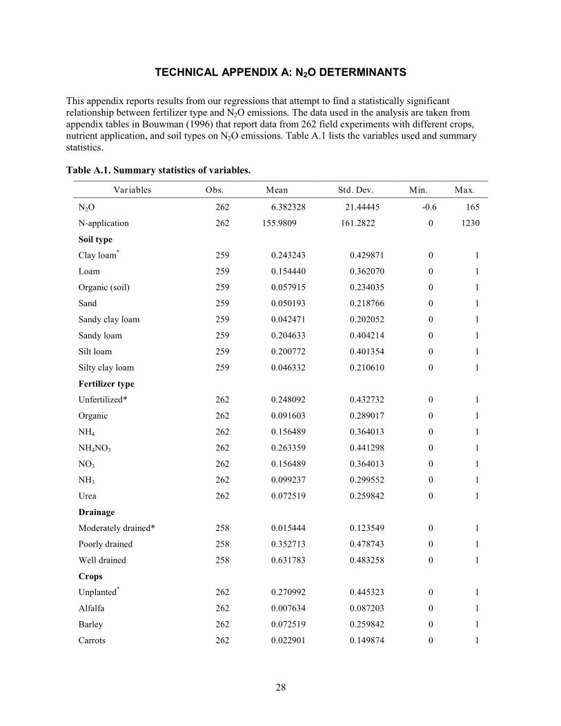
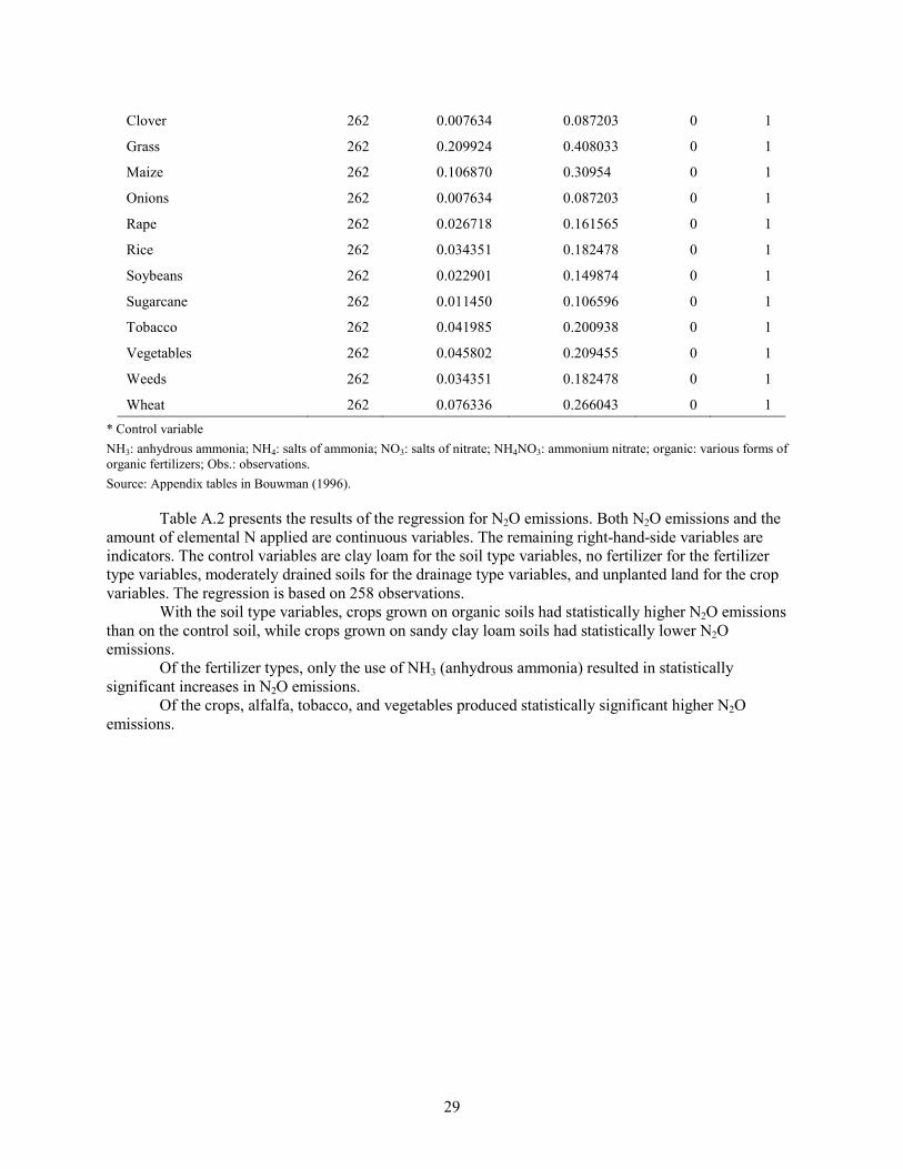
This appendix reports results from our regressions that attempt to find a statistically significant relationship between fertilizer type and N2O emissions. The data used in the analysis are taken from appendix tables in Bouwman (1996) that report data from 262 field experiments with different crops, nutrient application, and soil types on N2O emissions. Table A.1 lists the variables used and summary statistics.

Table A.1. Summary statistics of variables.

Var iables Obs. Mean Std. Dev. Min. Max.

N2O 262 6.382328 21.44445 -0.6 165

N-application 262 155.9809 161.2822 0 1230

Soil type

Clay loam* 259 0.243243 0.429871 0 1

Loam 259 0.154440 0.362070 0 1

Organic (soil) 259 0.057915 0.234035 0 1

Sand 259 0.050193 0.218766 0 1

Sandy clay loam 259 0.042471 0.202052 0 1

Sandy loam 259 0.204633 0.404214 0 1

Silt loam 259 0.200772 0.401354 0 1

Silty clay loam 259 0.046332 0.210610 0 1

Fertilizer type

Unfertilized* 262 0.248092 0.432732 0 1

Organic 262 0.091603 0.289017 0 1

NH4 262 0.156489 0.364013 0 1

NH4NO3 262 0.263359 0.441298 0 1

NO3 262 0.156489 0.364013 0 1

NH3 262 0.099237 0.299552 0 1

Urea 262 0.072519 0.259842 0 1

Drainage

Moderately drained* 258 0.015444 0.123549 0 1

Poorly drained 258 0.352713 0.478743 0 1

Well drained 258 0.631783 0.483258 0 1

Crops

Unplanted* 262 0.270992 0.445323 0 1

Alfalfa 262 0.007634 0.087203 0 1

Barley 262 0.072519 0.259842 0 1

Carrots 262 0.022901 0.149874 0 1

29

Clover 262 0.007634 0.087203 0 1

Grass 262 0.209924 0.408033 0 1

Maize 262 0.106870 0.30954 0 1

Onions 262 0.007634 0.087203 0 1

Rape 262 0.026718 0.161565 0 1

Rice 262 0.034351 0.182478 0 1

Soybeans 262 0.022901 0.149874 0 1

Sugarcane 262 0.011450 0.106596 0 1

Tobacco 262 0.041985 0.200938 0 1

Vegetables 262 0.045802 0.209455 0 1

Weeds 262 0.034351 0.182478 0 1

Wheat 262 0.076336 0.266043 0 1 * Control variable NH3: anhydrous ammonia; NH4: salts of ammonia; NO3: salts of nitrate; NH4NO3: ammonium nitrate; organic: various forms of organic fertilizers; Obs.: observations. Source: Appendix tables in Bouwman (1996).

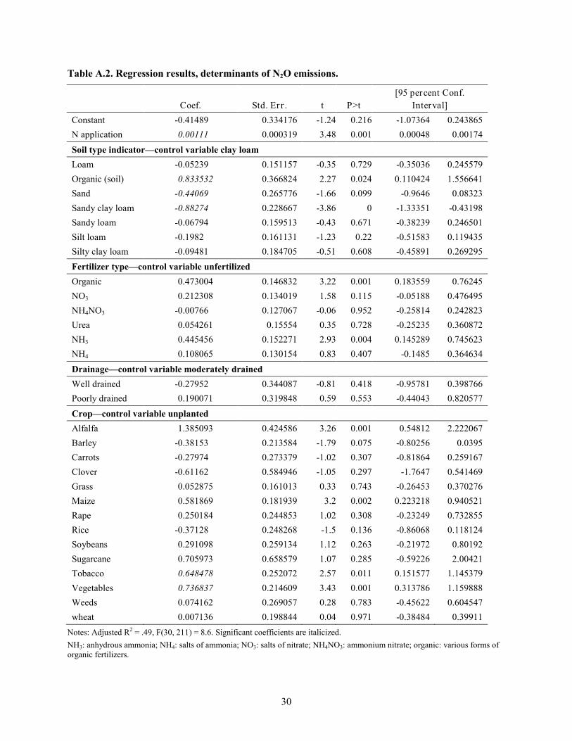
Table A.2 presents the results of the regression for N2O emissions. Both N2O emissions and the amount of elemental N applied are continuous variables. The remaining right-hand-side variables are indicators. The control variables are clay loam for the soil type variables, no fertilizer for the fertilizer type variables, moderately drained soils for the drainage type variables, and unplanted land for the crop variables. The regression is based on 258 observations.

With the soil type variables, crops grown on organic soils had statistically higher N2O emissions than on the control soil, while crops grown on sandy clay loam soils had statistically lower N2O emissions.

Of the fertilizer types, only the use of NH3 (anhydrous ammonia) resulted in statistically significant increases in N2O emissions.

Of the crops, alfalfa, tobacco, and vegetables produced statistically significant higher N2O emissions.

30

Table A.2. Regression results, determinants of N2O emissions.

Coef. Std. Er r . t P>t [95 percent Conf.

Interval] Constant -0.41489 0.334176 -1.24 0.216 -1.07364 0.243865 N application 0.00111 0.000319 3.48 0.001 0.00048 0.00174 Soil type indicator—control variable clay loam Loam -0.05239 0.151157 -0.35 0.729 -0.35036 0.245579 Organic (soil) 0.833532 0.366824 2.27 0.024 0.110424 1.556641 Sand -0.44069 0.265776 -1.66 0.099 -0.9646 0.08323 Sandy clay loam -0.88274 0.228667 -3.86 0 -1.33351 -0.43198 Sandy loam -0.06794 0.159513 -0.43 0.671 -0.38239 0.246501 Silt loam -0.1982 0.161131 -1.23 0.22 -0.51583 0.119435 Silty clay loam -0.09481 0.184705 -0.51 0.608 -0.45891 0.269295 Fertilizer type—control variable unfertilized Organic 0.473004 0.146832 3.22 0.001 0.183559 0.76245 NO3 0.212308 0.134019 1.58 0.115 -0.05188 0.476495 NH4NO3 -0.00766 0.127067 -0.06 0.952 -0.25814 0.242823 Urea 0.054261 0.15554 0.35 0.728 -0.25235 0.360872 NH3 0.445456 0.152271 2.93 0.004 0.145289 0.745623 NH4 0.108065 0.130154 0.83 0.407 -0.1485 0.364634 Drainage—control variable moderately drained Well drained -0.27952 0.344087 -0.81 0.418 -0.95781 0.398766 Poorly drained 0.190071 0.319848 0.59 0.553 -0.44043 0.820577 Crop—control variable unplanted Alfalfa 1.385093 0.424586 3.26 0.001 0.54812 2.222067 Barley -0.38153 0.213584 -1.79 0.075 -0.80256 0.0395 Carrots -0.27974 0.273379 -1.02 0.307 -0.81864 0.259167 Clover -0.61162 0.584946 -1.05 0.297 -1.7647 0.541469 Grass 0.052875 0.161013 0.33 0.743 -0.26453 0.370276 Maize 0.581869 0.181939 3.2 0.002 0.223218 0.940521 Rape 0.250184 0.244853 1.02 0.308 -0.23249 0.732855 Rice -0.37128 0.248268 -1.5 0.136 -0.86068 0.118124 Soybeans 0.291098 0.259134 1.12 0.263 -0.21972 0.80192 Sugarcane 0.705973 0.658579 1.07 0.285 -0.59226 2.00421 Tobacco 0.648478 0.252072 2.57 0.011 0.151577 1.145379 Vegetables 0.736837 0.214609 3.43 0.001 0.313786 1.159888 Weeds 0.074162 0.269057 0.28 0.783 -0.45622 0.604547 wheat 0.007136 0.198844 0.04 0.971 -0.38484 0.39911

Notes: Adjusted R2 = .49, F(30, 211) = 8.6. Significant coefficients are italicized. NH3: anhydrous ammonia; NH4: salts of ammonia; NO3: salts of nitrate; NH4NO3: ammonium nitrate; organic: various forms of organic fertilizers.

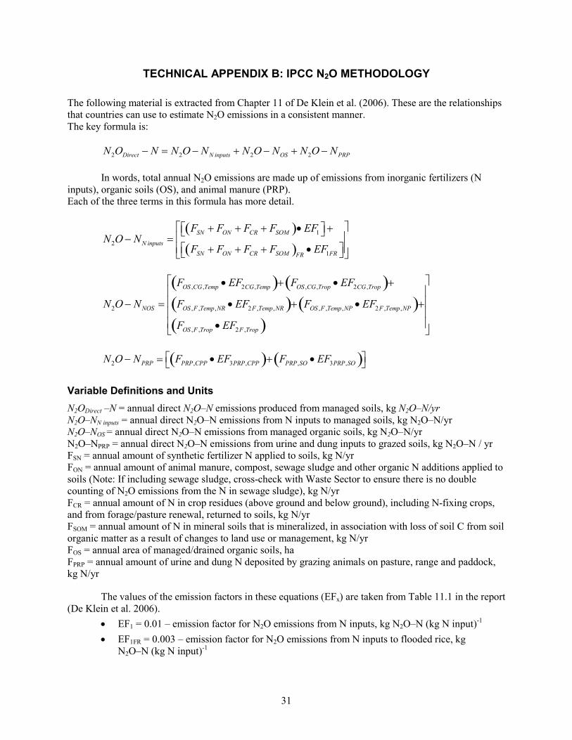
31

TECHNICAL APPENDIX B: IPCC N2O METHODOLOGY

The following material is extracted from Chapter 11 of De Klein et al. (2006). These are the relationships that countries can use to estimate N2O emissions in a consistent manner. The key formula is:

2 2 2 2Direct N inputs OS PRPN O N N O N N O N N O N− = − + − + −

In words, total annual N2O emissions are made up of emissions from inorganic fertilizers (N inputs), organic soils (OS), and animal manure (PRP). Each of the three terms in this formula has more detail.

( )( )

1

21

SN ON CR SOM

N inputsSN ON CR SOM FRFR

F F F F EFN O N

F F F F EF

+ + + • + − = + + + •

( ) ( )( ) ( )( )

, , 2 , , , 2 ,

2 , , , 2 , , , , , 2 , ,

, , 2 ,

OS CG Temp CG Temp OS CG Trop CG Trop

NOS OS F Temp NR F Temp NR OS F Temp NP F Temp NP

OS F Trop F Trop

F EF F EF

N O N F EF F EF

F EF

• + • + − = • + • + •

( ) ( )2 , 3 , , 3 ,PRP PRP CPP PRP CPP PRP SO PRP SON O N F EF F EF − = • + •

Variable Definitions and Units N2ODirect –N = annual direct N2O–N emissions produced from managed soils, kg N2O–N/yr N2O–NN inputs = annual direct N2O–N emissions from N inputs to managed soils, kg N2O–N/yr N2O–NOS = annual direct N2O–N emissions from managed organic soils, kg N2O–N/yr N2O–NPRP = annual direct N2O–N emissions from urine and dung inputs to grazed soils, kg N2O–N / yr FSN = annual amount of synthetic fertilizer N applied to soils, kg N/yr FON = annual amount of animal manure, compost, sewage sludge and other organic N additions applied to soils (Note: If including sewage sludge, cross-check with Waste Sector to ensure there is no double counting of N2O emissions from the N in sewage sludge), kg N/yr FCR = annual amount of N in crop residues (above ground and below ground), including N-fixing crops, and from forage/pasture renewal, returned to soils, kg N/yr FSOM = annual amount of N in mineral soils that is mineralized, in association with loss of soil C from soil organic matter as a result of changes to land use or management, kg N/yr FOS = annual area of managed/drained organic soils, ha FPRP = annual amount of urine and dung N deposited by grazing animals on pasture, range and paddock, kg N/yr

The values of the emission factors in these equations (EFx) are taken from Table 11.1 in the report (De Klein et al. 2006).

• EF1 = 0.01 – emission factor for N2O emissions from N inputs, kg N2O–N (kg N input)-1 • EF1FR = 0.003 – emission factor for N2O emissions from N inputs to flooded rice, kg

N2O–N (kg N input)-1

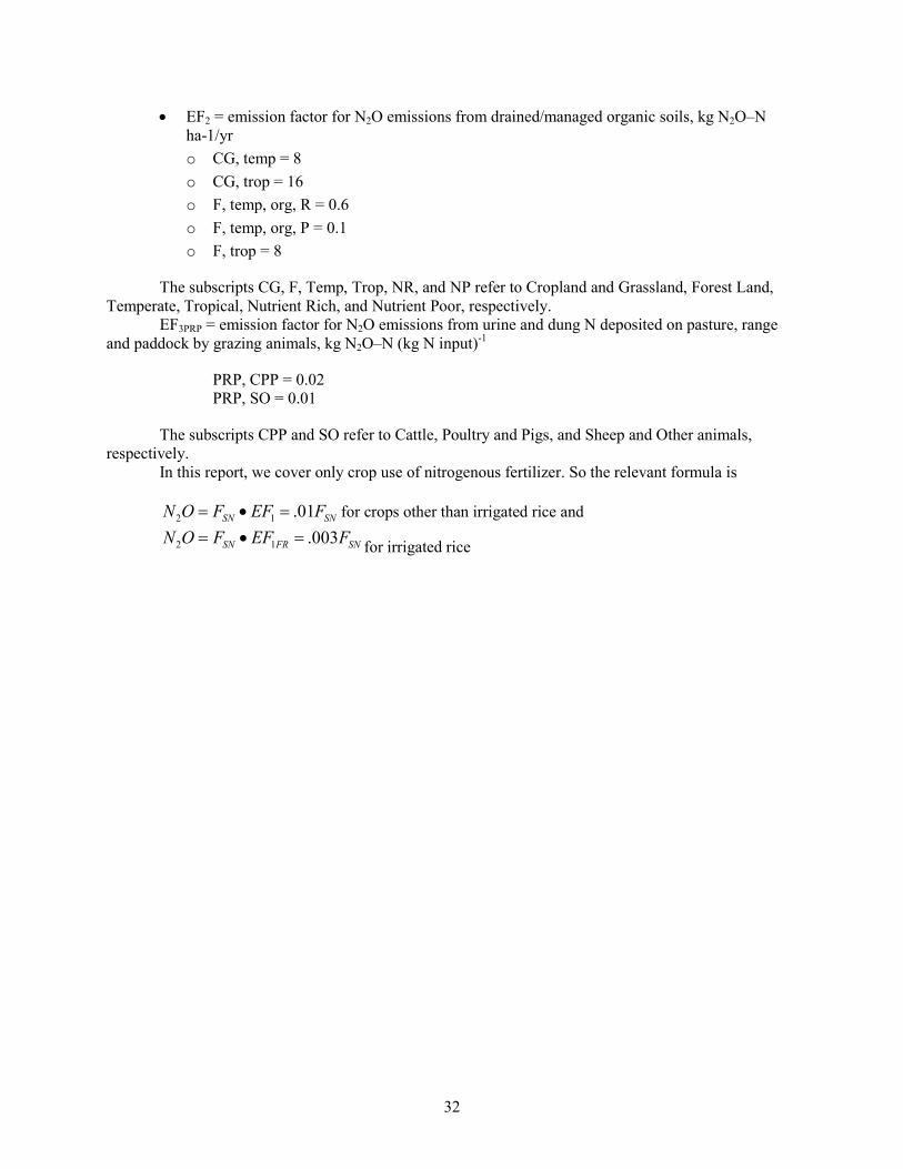
32

• EF2 = emission factor for N2O emissions from drained/managed organic soils, kg N2O–N ha-1/yr o CG, temp = 8 o CG, trop = 16 o F, temp, org, R = 0.6 o F, temp, org, P = 0.1 o F, trop = 8

The subscripts CG, F, Temp, Trop, NR, and NP refer to Cropland and Grassland, Forest Land, Temperate, Tropical, Nutrient Rich, and Nutrient Poor, respectively.

EF3PRP = emission factor for N2O emissions from urine and dung N deposited on pasture, range and paddock by grazing animals, kg N2O–N (kg N input)-1

PRP, CPP = 0.02 PRP, SO = 0.01

The subscripts CPP and SO refer to Cattle, Poultry and Pigs, and Sheep and Other animals, respectively.

In this report, we cover only crop use of nitrogenous fertilizer. So the relevant formula is

2 1 .01SN SNN O F EF F= • = for crops other than irrigated rice and

2 1 .003SN FR SNN O F EF F= • = for irrigated rice

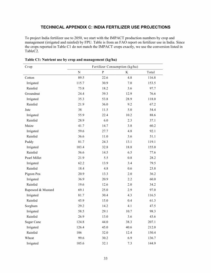
33

TECHNICAL APPENDIX C: INDIA FERTILIZER USE PROJECTIONS

To project India fertilizer use to 2050, we start with the IMPACT production numbers by crop and management (irrigated and rainfed) by FPU. Table is from an FAO report on fertilizer use in India. Since the crops reported in Table C1 do not match the IMPACT crops exactly, we use the conversion listed in TableC2.

Table C1: Nutrient use by crop and management (kg/ha)

Crop Fer tilizer Consumption (kg/ha) N P K Total

Cotton 89.5 22.6 4.8 116.8 Irrigated 115.7 30.9 7.0 153.5 Rainfed 75.8 18.2 3.6 97.7 Groundnut 24.4 39.3 12.9 76.6 Irrigated 35.3 53.8 28.9 118.0 Rainfed 21.9 36.0 9.2 67.2 Jute 38 11.5 5.0 54.4 Irrigated 55.9 22.4 10.2 88.6 Rainfed 28.9 6.0 2.3 37.1 Maize 41.7 14.7 3.8 60.2 Irrigated 59.6 27.7 4.8 92.1 Rainfed 36.6 11.0 3.6 51.1 Paddy 81.7 24.3 13.1 119.1 Irrigated 103.4 32.8 18.8 155.0 Rainfed 56.6 14.5 6.5 77.6 Pearl Millet 21.9 5.5 0.8 28.2 Irrigated 62.2 13.9 3.4 79.5 Rainfed 18.4 4.8 0.6 23.8 Pigeon Pea 20.9 13.3 2.0 36.2 Irrigated 36.9 20.9 2.2 60.0 Rainfed 19.6 12.6 2.0 34.2 Rapeseed & Mustard 69.1 25.0 2.9 97.0 Irrigated 81.7 30.4 4.3 116.5 Rainfed 45.9 15.0 0.4 61.3 Sorghum 29.2 14.2 4.1 47.5 Irrigated 58.5 29.1 10.7 98.3 Rainfed 26.9 13.0 3.6 43.6 Sugar Cane 124.8 44.0 38.3 207.1 Irrigated 126.4 45.0 40.6 212.0 Rainfed 106 32.0 12.4 150.4 Wheat 99.6 30.2 6.9 136.7 Irrigated 105.6 32.1 7.3 144.9

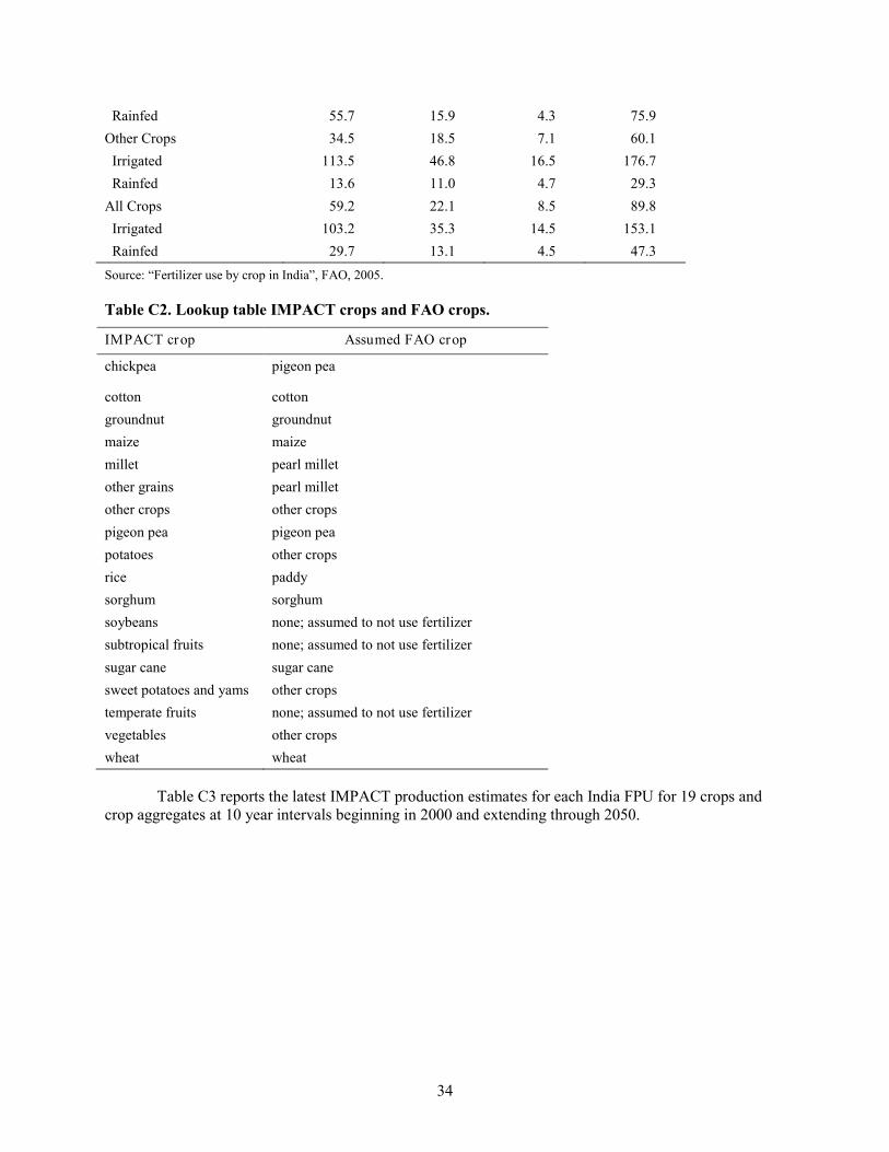
34

Rainfed 55.7 15.9 4.3 75.9 Other Crops 34.5 18.5 7.1 60.1 Irrigated 113.5 46.8 16.5 176.7 Rainfed 13.6 11.0 4.7 29.3 All Crops 59.2 22.1 8.5 89.8 Irrigated 103.2 35.3 14.5 153.1 Rainfed 29.7 13.1 4.5 47.3 Source: “Fertilizer use by crop in India”, FAO, 2005.

Table C2. Lookup table IMPACT crops and FAO crops.

IMPACT crop Assumed FAO crop

chickpea pigeon pea

cotton cotton groundnut groundnut maize maize millet pearl millet other grains pearl millet other crops other crops pigeon pea pigeon pea potatoes other crops rice paddy sorghum sorghum soybeans none; assumed to not use fertilizer subtropical fruits none; assumed to not use fertilizer sugar cane sugar cane sweet potatoes and yams other crops temperate fruits none; assumed to not use fertilizer vegetables other crops wheat wheat

Table C3 reports the latest IMPACT production estimates for each India FPU for 19 crops and crop aggregates at 10 year intervals beginning in 2000 and extending through 2050.

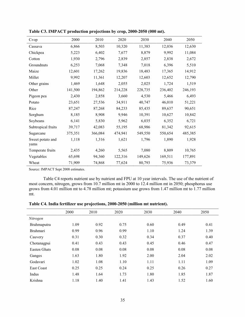
35

Table C3. IMPACT production projections by crop, 2000-2050 (000 mt).

Crop 2000 2010 2020 2030 2040 2050

Cassava 6,866 8,503 10,320 11,383 12,036 12,630 Chickpea 5,223 6,402 7,677 8,879 9,992 11,084 Cotton 1,930 2,796 2,839 2,857 2,838 2,672 Groundnuts 6,253 7,068 7,348 7,018 6,396 5,510 Maize 12,601 17,262 19,836 18,483 17,365 14,912 Millet 9,992 11,361 12,207 12,603 12,652 12,790 Other grains 1,469 1,648 2,055 2,025 1,724 1,519 Other 141,500 194,862 214,228 228,735 236,402 246,193 Pigeon pea 2,430 2,858 3,660 4,530 5,466 6,493 Potato 23,651 27,536 34,911 40,747 46,010 51,221 Rice 87,247 87,268 84,233 85,435 89,637 90,651 Sorghum 8,185 8,908 9,946 10,391 10,627 10,842 Soybeans 6,141 5,830 5,962 6,035 6,352 6,721 Subtropical fruits 39,717 42,083 55,195 68,986 81,342 92,615 Sugarcane 375,351 366,084 474,941 549,550 550,654 485,385 Sweet potato and yams

1,118 1,316 1,621 1,796 1,890 1,928

Temperate fruits 2,435 4,260 5,565 7,080 8,809 10,765 Vegetables 65,698 94,360 122,316 149,626 169,511 177,891 Wheat 71,909 74,868 77,624 80,793 75,936 73,379 Source: IMPACT Sept 2008 estimates.

Table C4 reports nutrient use by nutrient and FPU at 10 year intervals. The use of the nutrient of most concern, nitrogen, grows from 10.7 million mt in 2000 to 12.4 million mt in 2050; phosphorus use grows from 4.01 million mt to 4.78 million mt; potassium use grows from 1.47 million mt to 1.77 million mt.

Table C4. India fertilizer use projections, 2000-2050 (million mt nutrient).

2000 2010 2020 2030 2040 2050 Nitrogen Brahmaputra 1.09 0.92 0.75 0.60 0.49 0.41 Brahmari 0.99 0.96 0.99 1.10 1.24 1.39 Cauvery 0.31 0.30 0.32 0.34 0.37 0.40 Chotanagpui 0.41 0.43 0.43 0.45 0.46 0.47 Easten Ghats 0.08 0.08 0.08 0.08 0.08 0.08 Ganges 1.63 1.80 1.92 2.00 2.04 2.02 Godavari 1.02 1.08 1.10 1.11 1.11 1.09 East Coast 0.25 0.25 0.24 0.25 0.26 0.27 Indus 1.48 1.64 1.73 1.80 1.85 1.87 Krishna 1.18 1.40 1.41 1.43 1.52 1.60

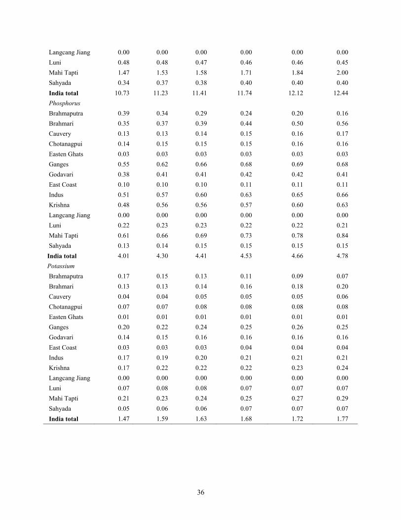
36

Langcang Jiang 0.00 0.00 0.00 0.00 0.00 0.00 Luni 0.48 0.48 0.47 0.46 0.46 0.45 Mahi Tapti 1.47 1.53 1.58 1.71 1.84 2.00 Sahyada 0.34 0.37 0.38 0.40 0.40 0.40 India total 10.73 11.23 11.41 11.74 12.12 12.44 Phosphorus Brahmaputra 0.39 0.34 0.29 0.24 0.20 0.16 Brahmari 0.35 0.37 0.39 0.44 0.50 0.56 Cauvery 0.13 0.13 0.14 0.15 0.16 0.17 Chotanagpui 0.14 0.15 0.15 0.15 0.16 0.16 Easten Ghats 0.03 0.03 0.03 0.03 0.03 0.03 Ganges 0.55 0.62 0.66 0.68 0.69 0.68 Godavari 0.38 0.41 0.41 0.42 0.42 0.41 East Coast 0.10 0.10 0.10 0.11 0.11 0.11 Indus 0.51 0.57 0.60 0.63 0.65 0.66 Krishna 0.48 0.56 0.56 0.57 0.60 0.63 Langcang Jiang 0.00 0.00 0.00 0.00 0.00 0.00 Luni 0.22 0.23 0.23 0.22 0.22 0.21 Mahi Tapti 0.61 0.66 0.69 0.73 0.78 0.84 Sahyada 0.13 0.14 0.15 0.15 0.15 0.15 India total 4.01 4.30 4.41 4.53 4.66 4.78 Potassium Brahmaputra 0.17 0.15 0.13 0.11 0.09 0.07 Brahmari 0.13 0.13 0.14 0.16 0.18 0.20 Cauvery 0.04 0.04 0.05 0.05 0.05 0.06 Chotanagpui 0.07 0.07 0.08 0.08 0.08 0.08 Easten Ghats 0.01 0.01 0.01 0.01 0.01 0.01 Ganges 0.20 0.22 0.24 0.25 0.26 0.25 Godavari 0.14 0.15 0.16 0.16 0.16 0.16 East Coast 0.03 0.03 0.03 0.04 0.04 0.04 Indus 0.17 0.19 0.20 0.21 0.21 0.21 Krishna 0.17 0.22 0.22 0.22 0.23 0.24 Langcang Jiang 0.00 0.00 0.00 0.00 0.00 0.00 Luni 0.07 0.08 0.08 0.07 0.07 0.07 Mahi Tapti 0.21 0.23 0.24 0.25 0.27 0.29 Sahyada 0.05 0.06 0.06 0.07 0.07 0.07 India total 1.47 1.59 1.63 1.68 1.72 1.77

37

TECHNICAL APPENDIX D: ESTIMATING THE CONTRIBUTION OF GROUNDWATER IRRIGATION PUMPING TO CO2 EMISSIONS

Introduction This note documents the methodology used to develop estimates of the contribution of groundwater pumping for irrigation to the CO2 emissions of India. It also reports detailed results.

Groundwater pumping requires energy. That energy can come from humans (using treadle pumps), animals, hydro, nuclear power and fossil fuels. Of these, only fossil fuels contribute significantly to CO2 emissions but they dominate the energy sources for groundwater pumping in India. Two different types of fossil fuels provide pumping energy – diesel and coal. Diesel fuel is transported close to the well location and used to power a diesel pump. Electric pumps rely on electricity produced for the most part from coal although hydro power accounts for about 13 percent and nuclear 3 percent (Source: Table 3.1 in Central Electricity Authority General Review 2005). This electricity is transported, sometimes long distances, to electric pumps near the fields to be irrigated.

Reference measures This section documents the various reference measures needed to convert crop production and implied irrigation water use to CO2 emissions.

Energy needed to lift 1000 m3 of water one meter

Using energy from either diesel fuel or coal releases CO2. The amount of CO2 released depends on the energy density of the fuel and the efficiency of the pumps. We start with the theoretical relationship that determines the energy needed to lift a mass as expressed in equation (0.1).

W mgh= (0.1) W = work (energy) in joules m = mass in kilograms g = gravitational constant = about 9.8 meters/sec2 h = height in meters 1 watt (W) = 1 joule (j) used per second

Using this relationship, we find that the energy required to lift 1000 m3 of water a distance of 1 meter is 2.724 kWh (9.8 * 106 J / (3.6 * 106 J/kWh)).8

This figure of 2.724 kWh reflects the energy embodied in the lifted water and does not include energy losses either in the pump itself or due to friction as the water is lifted through a pipe. In practice, the efficiency of this process is closer to 20 to 30 percent of the theoretical maximum. If we use a 30 percent efficiency rate (our baseline assumption), the effective energy use is 9.080 kWh per thousand cubic meters of water lifted one meter vertically.

CO2 released to lift 1000 m3 of water one meter

The amount of CO2 created in supplying this lift depends on the source of energy. Diesel does not have a unique chemical formulation so the mass and carbon content vary by mixture. A liter of standard diesel fuel contains approximately 0.732 kg carbon, a mass of approximately 0.85 kg and an energy content of

8 A liter of water weighs 1 kg. Thus 1,000 m3 = 106 kg. The energy required to lift this mass is 106 kg * 9.8 m/s2 * 1m = 9.8 * 106 J. For convenience, we convert this energy use rate to kilowatt hours (kWh), which are typically used to measure electric power usage. A watt measures the rate of energy usage where 1 W = 1 joule used per second. Thus a kWh = 1000 * 1 J/s * 3600 s/hour = 3.6 * 106 J. We can use this to convert the joules needed to lift a cubic meter 1 meter to kWh. The result is (9.8 * 106 J) / (3.6 * 106 J/kWh) = 2.724 kWh.

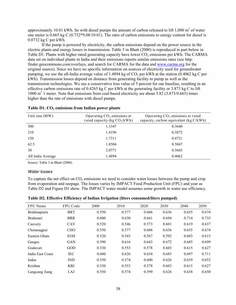
38

approximately 10.01 kWh. So with diesel pumps the amount of carbon released to lift 1,000 m3 of water one meter is 0.665 kg C (0.732*9.08/10.01). The ratio of carbon emissions to energy content for diesel is 0.0732 kg C per kWh.

If the pump is powered by electricity, the carbon emissions depend on the power source in the electric plants and energy losses in transmission. Table 3 in Bhatt (2000) is reproduced in part below in Table D1. Plants with higher rated generating capacity have lower CO2 emissions per kWh. The CARMA data set on individual plants in India and their emissions reports similar emissions rates (see http: finder.geocommons.com/overlays, and search for CARMA for the data and www.carma.org for the original source). Since we have no specific information on sources of electricity used for groundwater pumping, we use the all-India average value of 1.4894 kg of CO2 per kWh at the station (0.4062 kg C per kWh). Transmission losses depend on distance from generating facility to pump as well as the transmission technologies. We use a conservative loss value of 5 percent for our baseline, resulting in an effective carbon emissions rate of 0.4265 kg C per kWh at the generating facility or 3.873 kg C to lift 1000 m3 1 meter. Note that emissions from coal-based electricity are about 5.82 (3.873/0.665) times higher than the rate of emissions with diesel pumps.

Table D1. CO2 emissions from Indian power plants

Unit size (MW) Operating CO2 emissions at rated capacity (kg CO2/kWh)

Operating CO2 emissions at rated capacity, carbon equivalent (kg C/kWh)

500 1.3347 0.3640 210 1.4196 0.3872 120 1.7311 0.4721 62.5 1.8504 0.5047 30 2.0771 0.5665 All India Average 1.4894 0.4062 Source: Table 3 in Bhatt (2000).

Water losses

To capture the net effect on CO2 emissions we need to consider water losses between the pump and crop from evaporation and seepage. The losses varies by IMPACT Food Production Unit (FPU) and year as Table D2 and Figure D1 show. The IMPACT water model assumes some growth in water use efficiency.

Table D2. Effective Efficiency of Indian Irrigation (liters consumed/liters pumped)

FPU Name FPU Code 2000 2010 2020 2030 2040 2050 Brahmaputra BRT 0.550 0.577 0.606 0.636 0.655 0.674 Brahmari BRR 0.600 0.630 0.661 0.694 0.714 0.735 Cauvery CAV 0.520 0.546 0.573 0.601 0.619 0.637 Chotanagpui CHO 0.550 0.577 0.606 0.636 0.655 0.674 Eastern Ghats EGH 0.520 0.543 0.567 0.592 0.603 0.615 Ganges GAN 0.590 0.616 0.643 0.672 0.685 0.699 Godavari GOD 0.530 0.553 0.578 0.603 0.615 0.627 India East Coast IEC 0.600 0.626 0.654 0.683 0.697 0.711 Indus IND 0.550 0.574 0.600 0.626 0.639 0.652 Krishna KRI 0.530 0.553 0.578 0.603 0.615 0.627 Langcang Jiang LAJ 0.550 0.574 0.599 0.626 0.638 0.650

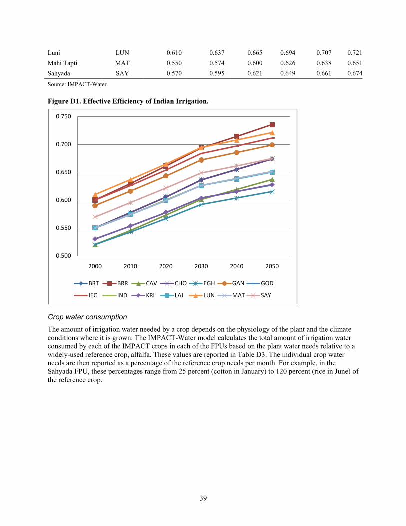
39

Luni LUN 0.610 0.637 0.665 0.694 0.707 0.721 Mahi Tapti MAT 0.550 0.574 0.600 0.626 0.638 0.651 Sahyada SAY 0.570 0.595 0.621 0.649 0.661 0.674 Source: IMPACT-Water.

Figure D1. Effective Efficiency of Indian Irrigation.

Crop water consumption

The amount of irrigation water needed by a crop depends on the physiology of the plant and the climate conditions where it is grown. The IMPACT-Water model calculates the total amount of irrigation water consumed by each of the IMPACT crops in each of the FPUs based on the plant water needs relative to a widely-used reference crop, alfalfa. These values are reported in Table D3. The individual crop water needs are then reported as a percentage of the reference crop needs per month. For example, in the Sahyada FPU, these percentages range from 25 percent (cotton in January) to 120 percent (rice in June) of the reference crop.

0.500

0.550

0.600

0.650

0.700

0.750

2000 2010 2020 2030 2040 2050

BRT BRR CAV CHO EGH GAN GOD

IEC IND KRI LAJ LUN MAT SAY

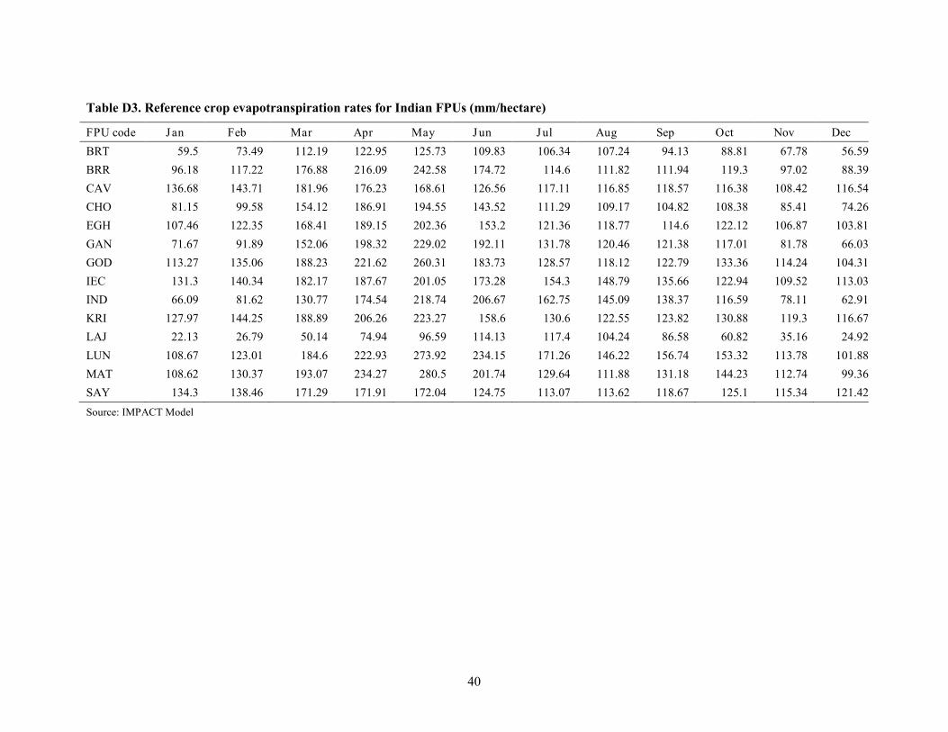
40

Table D3. Reference crop evapotranspiration rates for Indian FPUs (mm/hectare)

FPU code Jan Feb Mar Apr May Jun Jul Aug Sep Oct Nov Dec BRT 59.5 73.49 112.19 122.95 125.73 109.83 106.34 107.24 94.13 88.81 67.78 56.59 BRR 96.18 117.22 176.88 216.09 242.58 174.72 114.6 111.82 111.94 119.3 97.02 88.39 CAV 136.68 143.71 181.96 176.23 168.61 126.56 117.11 116.85 118.57 116.38 108.42 116.54 CHO 81.15 99.58 154.12 186.91 194.55 143.52 111.29 109.17 104.82 108.38 85.41 74.26 EGH 107.46 122.35 168.41 189.15 202.36 153.2 121.36 118.77 114.6 122.12 106.87 103.81 GAN 71.67 91.89 152.06 198.32 229.02 192.11 131.78 120.46 121.38 117.01 81.78 66.03 GOD 113.27 135.06 188.23 221.62 260.31 183.73 128.57 118.12 122.79 133.36 114.24 104.31 IEC 131.3 140.34 182.17 187.67 201.05 173.28 154.3 148.79 135.66 122.94 109.52 113.03 IND 66.09 81.62 130.77 174.54 218.74 206.67 162.75 145.09 138.37 116.59 78.11 62.91 KRI 127.97 144.25 188.89 206.26 223.27 158.6 130.6 122.55 123.82 130.88 119.3 116.67 LAJ 22.13 26.79 50.14 74.94 96.59 114.13 117.4 104.24 86.58 60.82 35.16 24.92 LUN 108.67 123.01 184.6 222.93 273.92 234.15 171.26 146.22 156.74 153.32 113.78 101.88 MAT 108.62 130.37 193.07 234.27 280.5 201.74 129.64 111.88 131.18 144.23 112.74 99.36 SAY 134.3 138.46 171.29 171.91 172.04 124.75 113.07 113.62 118.67 125.1 115.34 121.42 Source: IMPACT Model

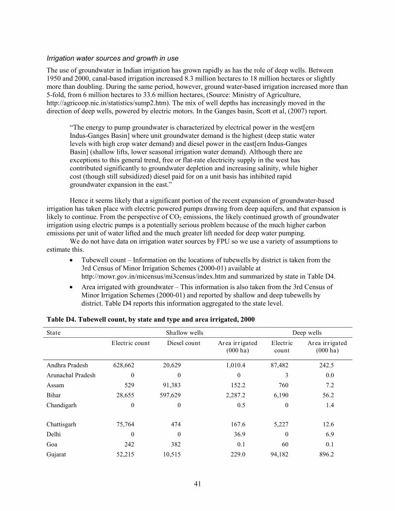
41

Irrigation water sources and growth in use

The use of groundwater in Indian irrigation has grown rapidly as has the role of deep wells. Between 1950 and 2000, canal-based irrigation increased 8.3 million hectares to 18 million hectares or slightly more than doubling. During the same period, however, ground water-based irrigation increased more than 5-fold, from 6 million hectares to 33.6 million hectares, (Source: Ministry of Agriculture, http://agricoop.nic.in/statistics/sump2.htm). The mix of well depths has increasingly moved in the direction of deep wells, powered by electric motors. In the Ganges basin, Scott et al, (2007) report.

“The energy to pump groundwater is characterized by electrical power in the west[ern Indus-Ganges Basin] where unit groundwater demand is the highest (deep static water levels with high crop water demand) and diesel power in the east[ern Indus-Ganges Basin] (shallow lifts, lower seasonal irrigation water demand). Although there are exceptions to this general trend, free or flat-rate electricity supply in the west has contributed significantly to groundwater depletion and increasing salinity, while higher cost (though still subsidized) diesel paid for on a unit basis has inhibited rapid groundwater expansion in the east.”

Hence it seems likely that a significant portion of the recent expansion of groundwater-based irrigation has taken place with electric powered pumps drawing from deep aquifers, and that expansion is likely to continue. From the perspective of CO2 emissions, the likely continued growth of groundwater irrigation using electric pumps is a potentially serious problem because of the much higher carbon emissions per unit of water lifted and the much greater lift needed for deep water pumping.

We do not have data on irrigation water sources by FPU so we use a variety of assumptions to estimate this.

• Tubewell count – Information on the locations of tubewells by district is taken from the 3rd Census of Minor Irrigation Schemes (2000-01) available at http://mowr.gov.in/micensus/mi3census/index.htm and summarized by state in Table D4.

• Area irrigated with groundwater – This information is also taken from the 3rd Census of Minor Irrigation Schemes (2000-01) and reported by shallow and deep tubewells by district. Table D4 reports this information aggregated to the state level.

Table D4. Tubewell count, by state and type and area irrigated, 2000

State Shallow wells Deep wells Electr ic count Diesel count Area ir r igated

(000 ha) Electr ic count

Area ir r igated (000 ha)

Andhra Pradesh 628,662 20,629 1,010.4 87,482 242.5 Arunachal Pradesh 0 0 0 3 0.0 Assam 529 91,383 152.2 760 7.2 Bihar 28,655 597,629 2,287.2 6,190 56.2 Chandigarh 0 0 0.5 0 1.4

Chattisgarh 75,764 474 167.6 5,227 12.6 Delhi 0 0 36.9 0 6.9 Goa 242 382 0.1 60 0.1 Gujarat 52,215 10,515 229.0 94,182 896.2

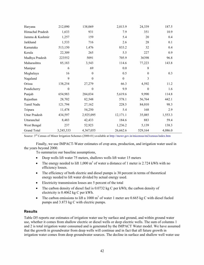
42

Haryana 212,090 138,069 2,013.9 24,339 187.5 Himachal Pradesh 1,633 931 7.9 351 10.9 Jammu & Kashmir 1,257 159 5.4 20 0.4 Jarkhand 1,533 716 2.6 28 0.1 Karnataka 513,150 1,476 833.2 32 0.4 Kerala 22,309 265 5.5 227 0.9 Madhya Pradesh 223552 5091 705.9 36398 96.8 Maharashtra 85,183 3,543 114.6 77,223 143.8 Manipur 6 69 0.0 8 Meghalaya 16 0 0.5 0 0.3 Nagaland 9 0 0 3 Orissa 138,254 27,279 66.3 4,592 11.2 Pondicherry 0 0 9.9 0 1.6 Punjab 654,983 284,034 5,619.6 9,990 114.8 Rajasthan 28,702 82,548 578.1 56,764 442.1 Tamil Nadu 121,794 27,162 228.5 84,010 98.3 Tripura 11,478 54,250 5.4 168 2.9 Uttar Pradesh 434,597 2,925,095 12,171.1 35,085 1,553.3 Uttaranchal 8,483 42,433 184.6 883 59.4 West Bengal 237 52,923 1,236.2 5,139 138.3 Grand Total 3,245,333 4,367,055 26,662.6 529,164 4,086.0 Source: 3rd Census of Minor Irrigation Schemes (2000-01) available at http://mowr.gov.in/micensus/mi3census/index.htm

Finally, we use IMPACT-Water estimates of crop area, production, and irrigation water used in the years beyond 2000.

To summarize our baseline assumptions, • Deep wells lift water 75 meters, shallows wells lift water 15 meters • The energy needed to lift 1,000 m3 of water a distance of 1 meter is 2.724 kWh with no

efficiency losses. • The efficiency of both electric and diesel pumps is 30 percent in terms of theoretical

energy needed to lift water divided by actual energy used. • Electricity transmission losses are 5 percent of the total • The carbon density of diesel fuel is 0.0732 kg C per kWh; the carbon density of

electricity is 0.4062 kg C per kWh. • The carbon emissions to lift a 1000 m3 of water 1 meter are 0.665 kg C with diesel fueled

pumps and 3.873 kg C with electric pumps.

Results Table D5 reports our estimates of irrigation water use by surface and ground, and within ground water use, whether it comes from shallow electric or diesel wells or deep electric wells. The sum of columns 1 and 2 is total irrigation water consumed and is generated by the IMPACT Water model. We have assumed that the growth in groundwater from deep wells will continue and in fact that all future growth in irrigation water comes from deep groundwater sources. The decline in surface and shallow well water use

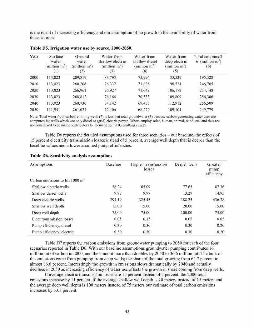
43

is the result of increasing efficiency and our assumption of no growth in the availability of water from these sources.

Table D5. Irrigation water use by source, 2000-2050.

Year Sur face water

(million m3) (1)

Ground water

(million m3) (2)

Water from shallow electr ic

(million m3) (3)

Water from shallow diesel (million m3)

(4)

Water from deep electr ic (million m3)

(5)

Total columns 3-6 (million m3)

(6)

2000 113,023 209,819 83,795 75,994 35,539 195,328 2010 113,023 260,206 76,337 71,836 98,531 246,705 2020 113,023 266,961 76,927 71,049 106,172 254,148 2030 113,023 268,812 76,164 70,333 109,809 256,306 2040 113,023 268,730 74,142 69,455 112,912 256,509 2050 111,941 261,024 72,406 68,272 109,101 249,779 Note: Total water from carbon-emitting wells (7) is less that total groundwater (3) because carbon-generating water uses are computed for wells which use only diesel or (grid) electric power. Others employ solar, human, animal, wind, etc. and thus are not considered to be major contributors to demand for GHG emitting energy.

Table D6 reports the detailed assumptions used for three scenarios – our baseline, the effects of 15 percent electricity transmission losses instead of 5 percent, average well depth that is deeper than the baseline values and a lower assumed pump efficiencies.

Table D6. Sensitivity analysis assumptions

Assumptions Baseline Higher transmission losses

Deeper wells Greater pump

efficiency Carbon emissions to lift 1000 m3 Shallow electric wells 58.24 65.09 77.65 87.36 Shallow diesel wells 9.97 9.97 13.29 14.95 Deep electric wells 291.19 325.45 388.25 436.78 Shallow well depth 15.00 15.00 20.00 15.00 Deep well depth 75.00 75.00 100.00 75.00 Elect transmission losses 0.05 0.15 0.05 0.05 Pump efficiency, diesel 0.30 0.30 0.30 0.20 Pump efficiency, electric 0.30 0.30 0.30 0.20

Table D7 reports the carbon emissions from groundwater pumping to 2050 for each of the four scenarios reported in Table D6. With our baseline assumptions groundwater pumping contributes 16 million mt of carbon in 2000, and the amount more than doubles by 2050 to 36.6 million mt. The bulk of the emissions come from pumping from deep wells; the share of the total growing from 64.7 percent to almost 86.6 percent. Interestingly the growth in emissions slows dramatically by 2040 and actually declines in 2050 as increasing efficiency of water use offsets the growth in share coming from deep wells.

If average electric transmission losses are 15 percent instead of 5 percent, the 2000 total emissions increase by 11 percent. If the average shallow well depth is 20 meters instead of 15 meters and the average deep well depth is 100 meters instead of 75 meters our estimate of total carbon emissions increases by 33.3 percent.

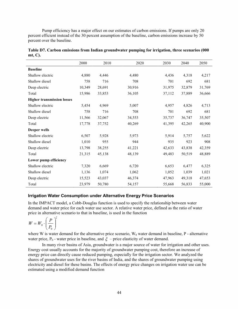
44

Pump efficiency has a major effect on our estimates of carbon emissions. If pumps are only 20 percent efficient instead of the 30 percent assumption of the baseline, carbon emissions increase by 50 percent over the baseline.

Table D7. Carbon emissions from Indian groundwater pumping for irrigation, three scenarios (000 mt, C).

2000 2010 2020 2030 2040 2050 Baseline Shallow electric 4,880 4,446 4,480 4,436 4,318 4,217 Shallow diesel 758 716 708 701 692 681 Deep electric 10,349 28,691 30,916 31,975 32,879 31,769 Total 15,986 33,853 36,105 37,112 37,889 36,666 Higher transmission losses Shallow electric 5,454 4,969 5,007 4,957 4,826 4,713 Shallow diesel 758 716 708 701 692 681 Deep electric 11,566 32,067 34,553 35,737 36,747 35,507 Total 17,778 37,752 40,269 41,395 42,265 40,900 Deeper wells Shallow electric 6,507 5,928 5,973 5,914 5,757 5,622 Shallow diesel 1,010 955 944 935 923 908 Deep electric 13,798 38,255 41,221 42,633 43,838 42,359 Total 21,315 45,138 48,139 49,483 50,519 48,889 Lower pump efficiency Shallow electric 7,320 6,669 6,720 6,653 6,477 6,325 Shallow diesel 1,136 1,074 1,062 1,052 1,039 1,021 Deep electric 15,523 43,037 46,374 47,963 49,318 47,653 Total 23,979 50,780 54,157 55,668 56,833 55,000

Irrigation Water Consumption under Alternative Energy Price Scenarios In the IMPACT model, a Cobb-Douglas function is used to specify the relationship between water demand and water price for each water use sector. A relative water price, defined as the ratio of water price in alternative scenario to that in baseline, is used in the function

ξ

⋅=

00 P

PWW

where W is water demand for the alternative price scenario, W0 water demand in baseline, P - alternative water price, P0 - water price in baseline, and ξ – price elasticity of water demand.

In many river basins of Asia, groundwater is a major source of water for irrigation and other uses. Energy cost usually accounts for the majority of groundwater pumping cost, therefore an increase of energy price can directly cause reduced pumping, especially for the irrigation sector. We analyzed the shares of groundwater uses for the river basins of India, and the shares of groundwater pumping using electricity and diesel for these basins. The effects of energy price changes on irrigation water use can be estimated using a modified demand function

45

( ) ( )[ ]ξ

θθα

⋅∆++∆+⋅⋅=0

0 11PPPPWW ddee

where α is the share of groundwater in total water use, eP∆ the increase of electricity price, dP∆ the

increase of diesel price, eθ the share of groundwater pumping using electricity, and dθ the share of groundwater pumping using diesel.

Workflow process Computing the total amount of carbon emissions requires determining how much water is coming from the various sources and then multiplying that by the emission rates for each of them. We consider four sources for irrigation water: surface water (no emissions), shallow diesel wells, shallow electric wells, and deep electric wells.

We begin by computing the total amount of water needed as projected by the IMPACT-water model. This means that we take the total beneficial irrigation amount and divide it by the assumed irrigation efficiency. The next task is to split the total amount of water needed into the contributions from the various sources. Since we assume no growth in capacity from surface water or shallow wells, these are assumed to provide (at most) the same amount as in the baseline period of 2000. That is, the amount of water that could be supplied by surface water is subtracted from the amount needed. If more water is needed, the shallow well capacity is removed. Any remaining needs are then met by the deep wells. The allocation between diesel and electric pumping for the shallow wells is done simply by multiplying the shallow water pumped by the fraction of diesel and electric pumps, respectively, among all shallow well pumps. (There is a small fraction of shallow pumping that is done by other means.)

The remaining matter is to establish the baseline capacities for surface water and shallow wells. We have data for several major states indicating the amount of cropland that is groundwater irrigated and the net irrigated area overall. From these, we compute the fraction of irrigated land that is groundwater irrigated. By assuming, for simplicity, that the water usage is constant between the major types of irrigation, the surface water capacity is computed by taking the total water needed in 2000 and multiplying by one minus the fraction of groundwater irrigated area. The remainder, then, comes from groundwater.

The baseline shallow well capacity is computed based on data from the Minor Irrigation Survey which indicate how much land is irrigated by shallow wells and by deep wells. Again, assuming relatively consistent water usage rates, the water provided by shallow wells is considered to be the total groundwater in 2000 multiplied by the fraction of area served by the shallow wells.

Details of the arithmetic are summarized as follows: Groundwater fraction = groundwater irrigated area / net irrigated area Baseline ground water =extra water needed in 2000 * (groundwater fraction) shallow fraction = shallow irrigated area / (deep irrigated area + shallow irrigated area) baseline shallow water = baseline ground water * shallow fraction baseline surface water = extra water needed in 2000 * (1.0 - groundwater fraction) total water needed = extra water needed / FPU water efficiency Deep carbon = deep water needed * carbon cost of deep Shallow carbon = shallow water needed * carbon cost of shallow, by diesel and electric Total carbon = shallow carbon + deep carbon Water needed = from a hierarchy: take total water needed, subtract out baseline surface water. If anything left: subtract out as much as is needed for baseline shallow water. If anything left, assign to deep water. Shallow diesel water needed = shallow water needed * (number of shallow diesel / total number of shallow wells) [note that total number of shallow wells is greater than diesel plus electric] Shallow electric water needed = shallow water needed * (number of shallow electric / total number of shallow wells)

46

References Bhatt, M. S. 2000. Energy efficiency and greenhouse emission burden from coal-fired electric power

plants- a case study of the Indian power sector. Energy Sources 22(7): 611-623. Scott, C., P. Narayana, et al. 2007. Groundwater in the Indus-Ganges Basin: Energy supply and pricing

impacts. Sri Lanka: International Water Management Institute.

47

REFERENCES

Bhatia, A., H. Pathak, and P. K. Aggarwal. 2004. Inventory of methane and nitrous oxide emissions from agricultural soils of India and their global warming potential. Current Science 87 (3): 317–324.

Bouwman, A. F. 1996. Direct emission of nitrous oxide from agricultural soils. Nutrient Cycling in Agroecosystems 46 (1): 53–70.

Central Electricity Authority. 2005. All India electricity statistics: General review. Delhi: Chandu Press.

De Klein, C., et al. 2006. IPCC guidelines for national greenhouse gas inventories. Agriculture, forestry and other land use, (4). Hayama, Japan: Intergovernmental Panel on Climate Change (IPCC).

Food and Agriculture Organization of the United Nations (FAO). 2004. World soil resources report: Carbon sequestration in dryland soils. Rome: FAO.

Forster, P., V. Ramaswamy, P. Artaxo, T. Berntsen, R. Betts, D.W. Fahey, J. Haywood, J. Lean, D.C. Lowe, G. Myhre, J. Nganga, R. Prinn, G. Raga, M. Schulz, and R. Van Dorland. 2007. Changes in atmospheric constituents and in radiative forcing. In Climate change 2007: The physical science basis. Contribution of working group I to the fourth assessment report of the Intergovernmental Panel on Climate Change, eds. S. Solomon, D. Qin, M. Manning, Z. Chen, M. Marquis, K.B. Averyt, M. Tignor, and H.L. Miller. Cambridge and New York: Cambridge University Press.

INRA. 2007. Why carbon storage is more stable in deep soil layers. http://www.international.inra.fr/press/carbon_storage_more_stable_deep_soil_layers. Accessed April 2009.

Lal, R. 2004. Soil carbon sequestration in India. Climatic Change 65 (3): 277–296.

Ministry of Agriculture, Government of India. Net area irrigated from different sources of irrigation and gross irrigated area (all India). http://agricoop.nic.in/statistics/sump2.htm. Accessed November 25, 2008.]

Nelson, A. 2007. Global accessibility model for travel time estimates to populated places of 250,000 persons or more. Ispra, Italy: Joint Research Centre of the European Commission.

Pathak, H., C. Li, and R. Wassmann. 2005. Greenhouse gas emissions from Indian rice fields: calibration and upscaling using the DNDC model. Biogeosciences 2 (2): 113–123.

Rosegrant M.W. S. Msangi, C. Ringler, T.B. Sulser, T. Zhu, and S.A. Cline. 2008. International model for policy analysis of agricultural commodities and trade (IMPACT): Model description. Washington, D.C.: International Food Policy Research Institute.

Willey, Z., and B. Chameides. 2007. Harnessing farms and forests in the low-carbon economy: How to create, measure, and verify greenhouse gas offsets. Durham, NC: Duke University Press.

World Resources Institute. 2009. Climate analysis indicators tool (CAIT) 6.0. Washington, DC: World Resources Institute.

You, L., and S. Wood. 2006. An entropy approach to spatial disaggregation of agricultural production. Agricultural Systems 90 (1–3): 329-347.

48

RECENT IFPRI DISCUSSION PAPERS

For earlier discussion papers, please go to www.ifpri.org/pubs/pubs.htm#dp. All discussion papers can be downloaded free of charge.

899. Rural non-farm income and inequality in Nigeria. Babatunde Omilola, 2009.

898. Lagging regions and development strategies: The case of Peru. James Thurlow, Samuel Morley, and Alejandro Nin Pratt, 2009.

897. Spatial networks, labor supply, and income dynamics: Evidence from Indonesian villages. Futoshi Yamauchi, Megumi Muto, Shyamal Chowdhury, Reno Dewina, and Sony Sumaryanto, 2009.

896. The evolution of an industrial cluster in China. Belton Fleisher, Dinghuan Hu, William McGuire, and Xiaobo Zhang, 2009.

895. Commodity price volatility and nutrition vulnerability. Monika Verma and Thomas W. Hertel, 2009

894. Measuring irrigation performance in Africa. Mark Svendsen, Mandy Ewing, and Siwa Msangi, 2009

893. Managing future oil revenues in Ghana: An assessment of alternative allocation options. Clemens Breisinger, Xinshen Diao, Rainer Schweickert, and Manfred Wiebelt, 2009.

892. Impact of water user associations on agricultural productivity in Chile. Nancy McCarthy and Tim Essam, 2009.

891. China’s growth and the agricultural exports of southern Africa. Nelson Villoria, Thomas Hertel, and Alejandro Nin-Pratt, 2009.

890. The impact of climate variability and change on economic growth and poverty in Zambia. James Thurlow, Tingju Zhu, and Xinshen Diao, 2009.

889. Navigating the perfect storm: Reflections on the food, energy, and financial crises. Derek Headey, Sangeetha Malaiyandi, and Shenggen Fan, 2009.

888. How important is a regional free trade area for southern Africa? Potential impacts and structural constraints. Alejandro Nin Pratt, Xinshen Diao, and Yonas Bahta, 2009.

887. Determinant of smallholder farmer labor allocation decisions in Uganda. Fred Bagamba, Kees Burger, and Arie Kuyvenhoven, 2009.

886. The potential cost of a failed Doha Round. Antoine Bouët and David Laborde, 2009.

885. Mapping South African farming sector vulnerability to climate change and variability: A subnational assessment. Glwadys Aymone Gbetibouo and Claudia Ringler, 2009.

884. How does food price increase affect Ugandan households? An augmented multimarket approach. John M. Ulimwengu and Racha Ramadan, 2009.

883. Linking urban consumers and rural farmers in India: A comparison of traditional and modern food supply chains. Bart Minten, Thomas Reardon, and Anneleen Vandeplas, 2009.

882. Promising Approaches to Address the Needs of Poor Female Farmers: Resources, Constraints, and Interventions. Agnes R. Quisumbing and Lauren Pandolfelli, 2009.

881. Natural Disasters, Self-Insurance, and Human Capital Investment: Evidence from Bangladesh, Ethiopia, and Malawi. Futoshi Yamauchi, Yisehac Yohannes, and Agnes Quisumbing, 2009.

880. Risks, ex-ante actions, and public assistance: Impacts of natural disasters on child schooling in Bangladesh, Ethiopia, and Malawi. Futoshi Yamauchi, Yisehac Yohannes, and Agnes Quisumbing, 2009.

879. Measuring child labor: Comparisons between hours data and subjective measures. Andrew Dillon, 2009.

878. The effects of political reservations for women on local governance and rural service provision: Survey evidence from Karnataka. Katharina Raabe, Madhushree Sekher, and Regina Birner, 2009.

INTERNATIONAL FOOD POLICY RESEARCH INSTITUTE

www.ifpri.org

IFPRI HEADQUARTERS

2033 K Street, NW Washington, DC 20006-1002 USA Tel.: +1-202-862-5600 Fax: +1-202-467-4439 Email: ifpri@cgiar.org

IFPRI ADDIS ABABA

P. O. Box 5689 Addis Ababa, Ethiopia Tel.: +251 11 6463215 Fax: +251 11 6462927 Email: ifpri-addisababa@cgiar.org

IFPRI NEW DELHI

CG Block, NASC Complex, PUSA New Delhi 110-012 India Tel.: 91 11 2584-6565 Fax: 91 11 2584-8008 / 2584-6572 Email: ifpri-newdelhi@cgiar.org