
Global Warming and the daunting challenge of Climate-Ecosystem Feedbacks
The University of Toronto
October 20, 2005
John Harte
University of California, Berkeley

With graduate students:
Scott Saleska, Marc Fischer, Jennifer Dunne, Margaret Torn, Becky Shaw, Michael Loik, Molly Smith, Lara Kueppers, Karin Shen, Perry deValpine, Ann Kinzig, Fang Ru Chang, Julia Klein
and undergraduates:
Tracy Perfors, Liz Alter, Francesca Saavedra, Susan McDowell, Brian Feifarek, Hadley Renkin, Chris Still, Laurie Tucker, Agnieska Rawa, Vanessa Price, Julia Harte, Wendy Brown, Susan Mahler, Erika Hoffman, Jim Williams, Eric Sparling, Jennifer Hazen, Jim Downing, Sheridan Pauker, Billy Barr, Kathy Northrop, Ann and Dave Zweig, Kevin Taylor, Aaron Soule, Andrew Wilcox, Mike Geluardi, Annabelle Singer, Sarah McCarthy
And with Financial Support from NSF, DOE, USDA, NASA, USEPA,
Outline of this talk
1.A quick overview of global warming
2. A global view of climate-ecosystem interactions and feedbacks
3. A local view: results from the RMBL meadow-warming experiment

Sunlight
Heat
Greenhouse gases
Heat
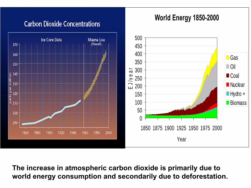
The increase in atmospheric carbon dioxide is primarily due to world energy consumption and secondarily due to deforestation.
World Energy 1850-2000
050
100150200250300350400450500
1850 1875 1900 1925 1950 1975 2000
YearE
J/ye
ar
GasOilCoalNuclearHydro +Biomass
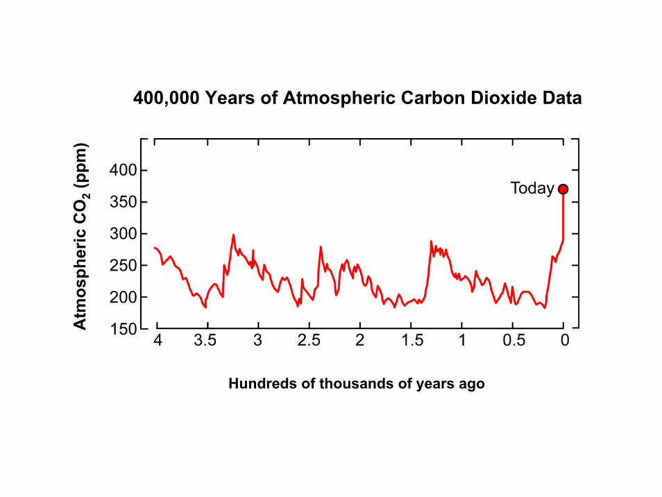
Hundreds of thousands of years ago
400,000 Years of Atmospheric Carbon Dioxide DataA
tmos
pher
ic C
O2
(ppm
)
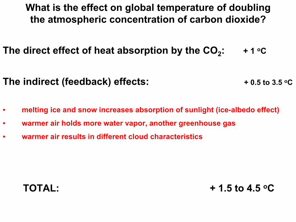
What is the effect on global temperature of doubling the atmospheric concentration of carbon dioxide?
The direct effect of heat absorption by the CO2: + 1 oC
The indirect (feedback) effects: + 0.5 to 3.5 oC
• melting ice and snow increases absorption of sunlight (ice-albedo effect)
• warmer air holds more water vapor, another greenhouse gas
• warmer air results in different cloud characteristics
TOTAL: + 1.5 to 4.5 oC

Temperatures During the Past Ice Age
oF oC
Thousands of years ago
Should we worry about +4 oC change?

O CO F
1000 Years of Northern Hemisphere Temperature Data
year

Fingerprint of Global Warming
•Stratosphere cools as surface warms
•Temperature rises faster at night than day
•Temperature rises faster in winter than summer
•High latitudes warm more than low latitudes
If global warming were caused by a brightening sun, then the stratosphere would warm and temperature rise would be greatest in daytime
Models predict, and the data show that:

IMPACTS OF GLOBAL WARMING
• Threats to Food Production (Diminished Water Supplies)
• Human Health Impacts (Heat Waves, Infectious Disease)
• Wildfire
• Sealevel Rise
• Ecological Effects:
Extinction Episode Comparable to K-T Boundary
Spread of Invasive Species
Coral Bleaching
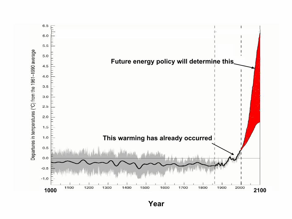
Future energy policy will determine this
This warming has already occurred
1000 2100
Year
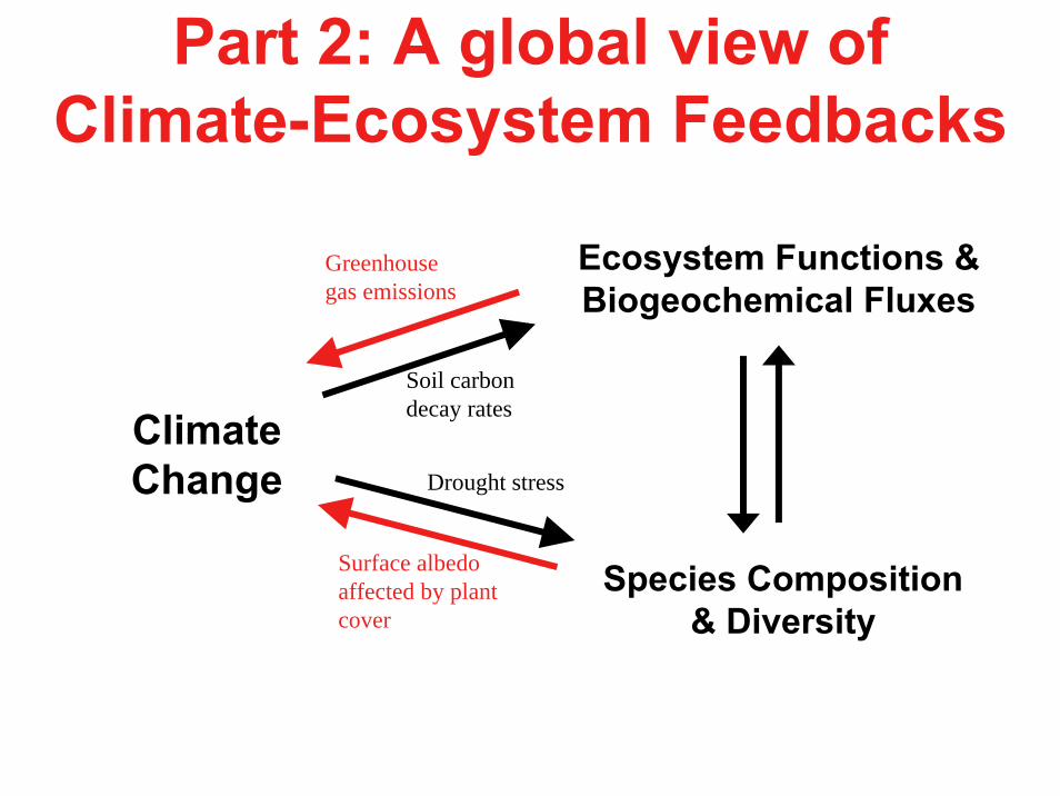
Part 2: A global view of Climate-Ecosystem Feedbacks
Climate Change
Species Composition & Diversity
Ecosystem Functions & Biogeochemical Fluxes
Surface albedoaffected by plant cover
Greenhouse gas emissions
Soil carbon decay rates
Drought stress

Retreat of N. American Ice Sheet
The model with rock and silt surface predicts slow retreat
Rate predicted w/ rock surface
Rat
e of
retr
eat
(km
y-1
)
Surface Absorption(1-albedo)
Actualrate
Rock, Silta = 0.4

Retreat of N. American Ice Sheet
The model with spruce trees predicts actual rate
Rate predicted w/ rock surface
Rat
e of
retr
eat
(km
y-1
)
Surface Absorption(1-albedo)
Spruce Treesa = 0.1
Actualrate
Rock, Silta = 0.4
Vegetation effect
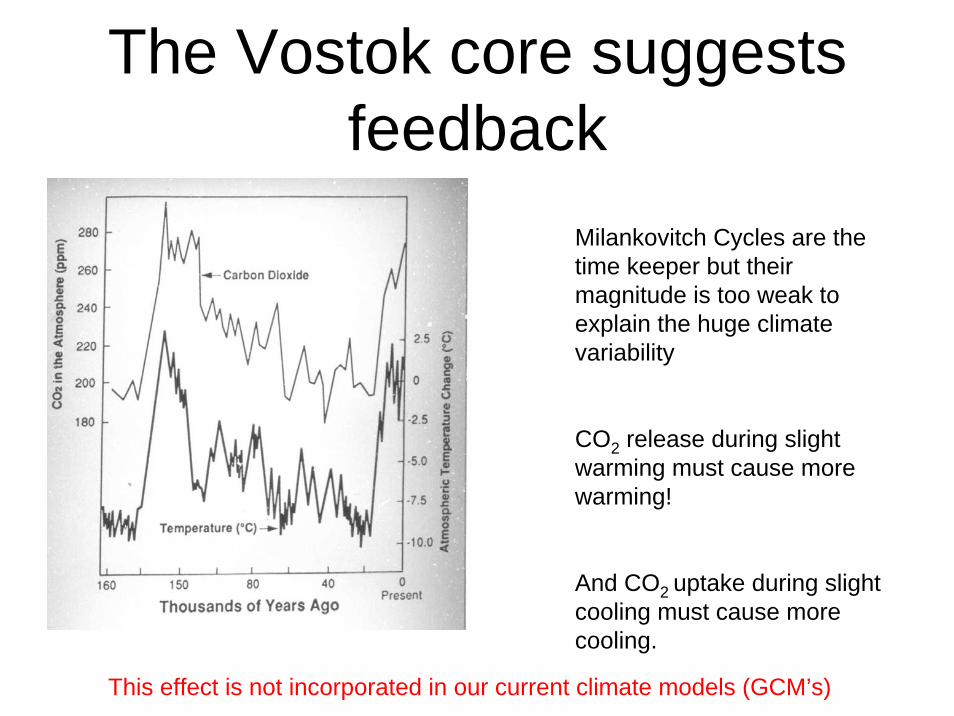
The Vostok core suggests feedback
Milankovitch Cycles are the time keeper but their magnitude is too weak to explain the huge climate variability
CO2 release during slight warming must cause more warming!
And CO2 uptake during slight cooling must cause more cooling.
This effect is not incorporated in our current climate models (GCM’s)

Slide 16
WB3 Wendy Brown, 2003-10-13

biosphere
HOW DO WE QUANTIFY FEEDBACK?
O = I + gI + ggI + gggI + ...
= I / (1 - g) if g < 1
If g < 0: O < I, negative feedbackIf g > 0, g < 1: O > I, positive feedback, stableIf g > 1: unstable positive feedback
Gain Factor (g)
Output Signal (O)
(e.g., full warming effect)
Input Signal (I)
(e.g., direct warming effect of GHG increase)
g = Σ (∂T/∂pi)(∂pi/∂T)
e.g., p1(T) = albedo of land surface, which may change if warming induces a changes in dominant vegetation
pi

FEEDBACK (CONTINUED)g < 0: O < I, negative feedback g > 0: O > I, positive feedback g > 1: Unstable
Feedback process Gain factor (g)
In current GCMs:water vapor 0.40 (0.28 - 0.52)ice and snow 0.09 (0.03 - 0.21)clouds 0.22 (-0.12 - 0.29)
total 0.71 (0.17 - 0.77)
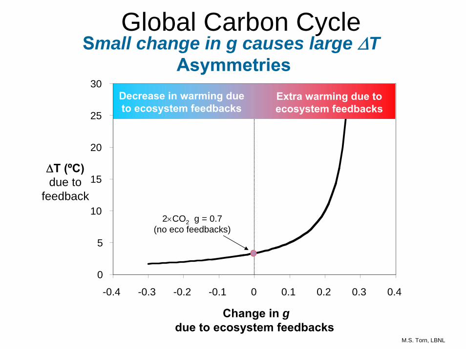
Climate change: ∆T=forcing effect/(1-g)
∆T = 1oC/(1 – 0.71) = 3.oC
0
5
10
15
20
25
30
-0.4 -0.3 -0.2 -0.1 0 0.1 0.2 0.3 0.4
2×CO2 g = 0.7(no eco feedbacks)
Extra warming due to ecosystem feedbacks
Decrease in warming due to ecosystem feedbacks
Global Carbon Cycle
ΔT (ºC)due to
feedback
Change in gdue to ecosystem feedbacks
Small change in g causes large ΔT Asymmetries
M.S. Torn, LBNL
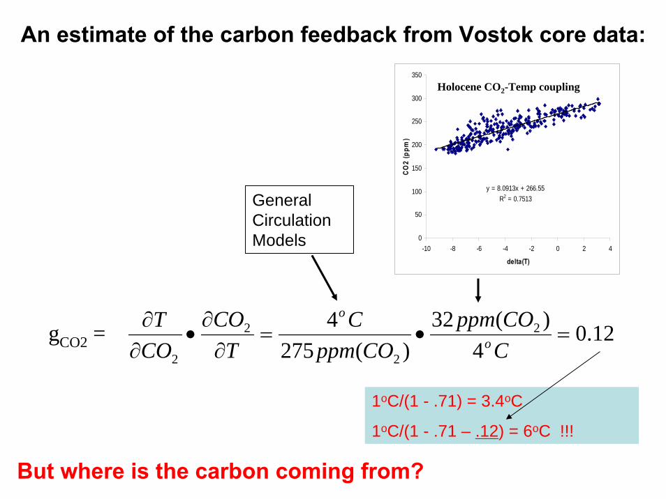
gCO2 = 12.04
)(32)(275
4 2
2
2
2
=•=∂
∂•
∂∂
CCOppm
COppmC
TCO
COT
o
o
An estimate of the carbon feedback from Vostok core data:
1oC/(1 - .71) = 3.4oC
1oC/(1 - .71 – .12) = 6oC !!!
y = 8.0913x + 266.55R2 = 0.7513
0
50
100
150
200
250
300
350
-10 -8 -6 -4 -2 0 2 4
delta(T)
CO2
(ppm
)
General Circulation Models
Holocene CO2-Temp coupling
But where is the carbon coming from?
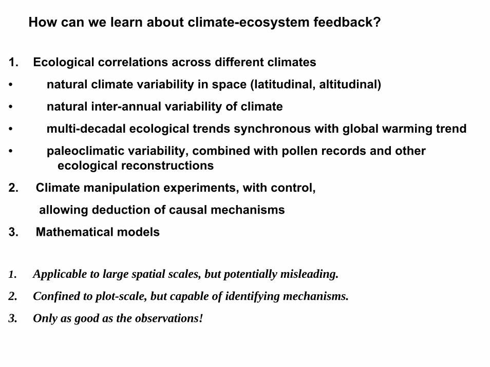
How can we learn about climate-ecosystem feedback?
1. Ecological correlations across different climates
• natural climate variability in space (latitudinal, altitudinal)
• natural inter-annual variability of climate
• multi-decadal ecological trends synchronous with global warming trend
• paleoclimatic variability, combined with pollen records and other ecological reconstructions
2. Climate manipulation experiments, with control,
allowing deduction of causal mechanisms
3. Mathematical models
1. Applicable to large spatial scales, but potentially misleading.
2. Confined to plot-scale, but capable of identifying mechanisms.
3. Only as good as the observations!

POSSIBLE LEVELS OF AGGREGATION
IN GLOBAL MODELS
Planet
Single big leaf
N=1
Biomes
Coarse Functional Groups
N ~ 10
Ecosystems
Functional Groups
N ~ 1000’s
Community Patch
Species assemblage
N ~ millions

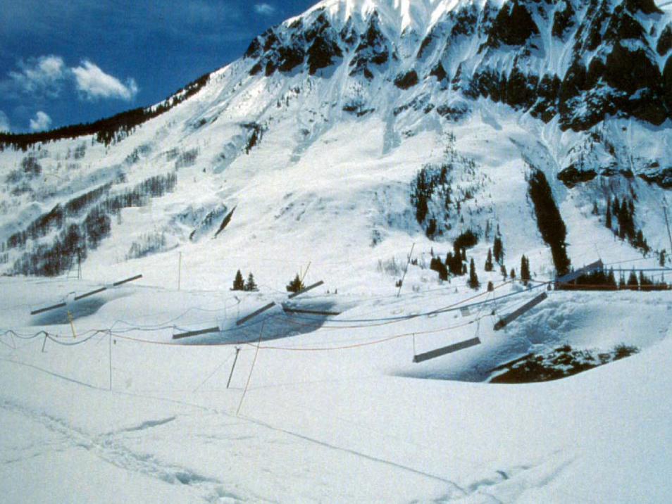
Part 3: A “longterm” warming experiment

Rocky Mt. Biological Laboratory, Gothic, ColoradoInfra-red heaters (22 W m-2). Soil is warmer, drier; Earlier snowmelt

Warming Treatment Effect: Forb Production Decreases. Sagebrush Production Increases.
% Change in areal cover
Warming− Control( )Control
•100%
Forbs
Harte and Shaw, Science, 1995
Sagebrush
-30
-15
0
15
30
Delphinium nelsonii in John Harte's global warming experiment
Julian date of snowmelt in upper zone100 110 120 130 140 150 160
Num
ber o
f flo
wer
ing
plan
ts in
plo
ts
0
100
200
300
400
500
600
700
H-1994H-1995
H-1996
H-1997
H-1998
H-1999
H-2000
H-2001H-2003
H-2004
H-2005
C-1994
C-1995
C-1996
C-1997
C-1998
C-1999
C-2000
C-2001
C-2003
C-2004
C-2005
r2 = .470p = .0004
Inouye data
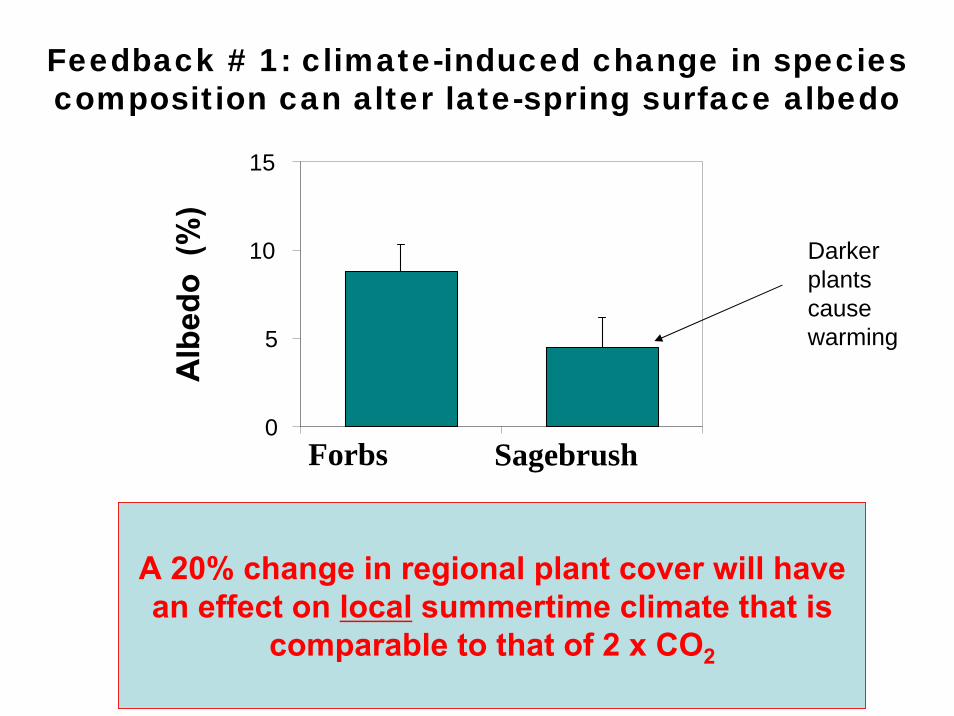
Feedback # 1: climate-induced change in species composition can alter late-spring surface albedo
Forbs Sagebrush
Alb
edo
(%)
A 20% change in regional plant cover will have an effect on local summertime climate that is
comparable to that of 2 x CO2
0
5
10
15
Darker plants cause warming

Met
hane
Upt
ake
(mg
CH
4m
-2d-1
)
Soil Moisture (%)
Feedback # 2: methane consumption influenced by soil moisture
negative feedbackpositive feedback
If warming → soil drying:
Torn and Harte, Biogeochemistry, 1995
SOIL ORGANIC CARBON
2
2.5
3
3.5
4
4.5
5
5.5
6
6.5
0 2 4 6 8 10
year since 1990
% s
oil c
arbo
n
Series1
Series2
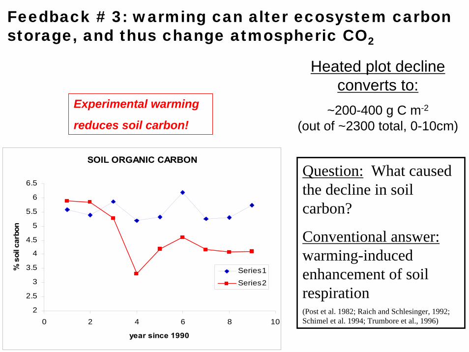
Feedback # 3: warming can alter ecosystem carbon storage, and thus change atmospheric CO2
Question: What caused the decline in soil carbon?
Conventional answer: warming-induced enhancement of soil respiration (Post et al. 1982; Raich and Schlesinger, 1992; Schimel et al. 1994; Trumbore et al., 1996)
Heated plot decline converts to:
~200-400 g C m-2
(out of ~2300 total, 0-10cm)
Experimental warming
reduces soil carbon!

What caused the decline in soil carbon? NOT a heating-induced increase in soil
respiration
y = 0.1925x + 0.17252R2 = 0.92
0.5
1.5
2.5
0 5 10 15
temp * moisture (o C g H2O/gsoil)
resp
iratio
n, μ
g C
g-1
soil
hr-1
Soil drying and soil warming have opposite effects
(evidence from laboratory soil incubation)
Full 5x5 factorial :0, 10, 13,18, 30 deg. C2, 10, 20, 30, 40 %H2O
Thus,
as T ↑, decomposition ↑
as M↓, decomposition ↓
No overall effect!
Saleska et al., Global Biogeochemical Cycles, 2002
Upper
LowerMid
Heated
1000
1500
2000
2500
3000
4 5 6 7Mean Annual Temp (deg C)
Soil
Org
anic
Car
bon
(gC
/m2)
Control
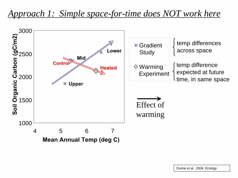
Approach 1: Simple space-for-time does NOT work here
GradientStudy
WarmingExperiment
Effect of warming
temp differences across space
temp difference expected at future time, in same space
Dunne et al., 2004, Ecology
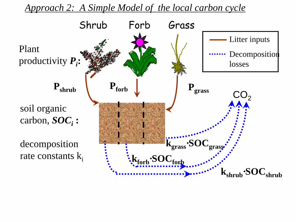
soil organic carbon, SOCi :
decomposition rate constants ki
Shrub Forb Grass
Pshrub Pforb Pgrass
kshrub·SOCshrub
kforb·SOCforb
kgrass·SOCgrass
Plant productivity Pi:
Litter inputs
Decomposition losses
Approach 2: A Simple Model of the local carbon cycle
CO2
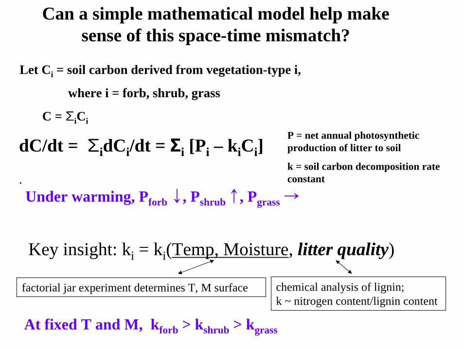
Key insight: ki = ki(Temp, Moisture, litter quality)
chemical analysis of lignin; k ~ nitrogen content/lignin content
Can a simple mathematical model help make sense of this space-time mismatch?
Let Ci = soil carbon derived from vegetation-type i,
where i = forb, shrub, grass
C = ΣiCi
dC/dt = ΣidCi/dt = Σi [Pi – kiCi]
. Under warming, Pforb ↓, Pshrub↑, Pgrass→
factorial jar experiment determines T, M surface
At fixed T and M, kforb > kshrub > kgrass
P = net annual photosynthetic production of litter to soil
k = soil carbon decomposition rate constant

2200
2000 3000 4000
2400
2600
SOC
(g C
m-2
)
2000 3000 4000 5000Predicted SOC
2000
B
uppermiddlelowerwarm contrl
contrlheat
AVGAVG
R2=0.84
Test of Simple Model for ambient Soil Organic Carbon
Predicted SOC
The equilibrium solution to the model accurately predicts ambient soil carbon levels across a climate gradient.
It fails to predict the transient response of carbon levels to heating.
So let’s look at the dynamic solution to the differential equations…
Saleska et al., Global Biogeochemical Cycles, 2002
Dunne et al., Ecology, 2004
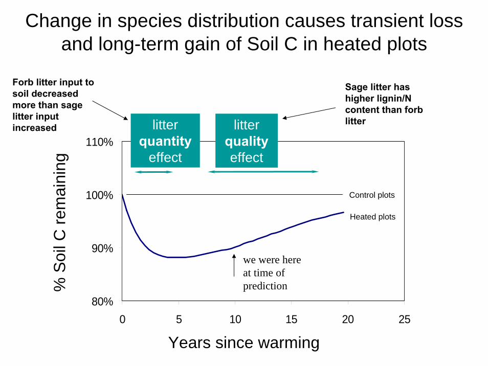
Change in species distribution causes transient loss and long-term gain of Soil C in heated plots
Years since warming
% S
oil C
rem
aini
ng
80%
90%
100%
110%
0 5 10 15 20 25
litter quality effect
litter quantity
effect
we were here at time of prediction
Forb litter input to soil decreased more than sage litter input increased
Sage litter has higher lignin/N content than forblitter
Heated plots
Control plots
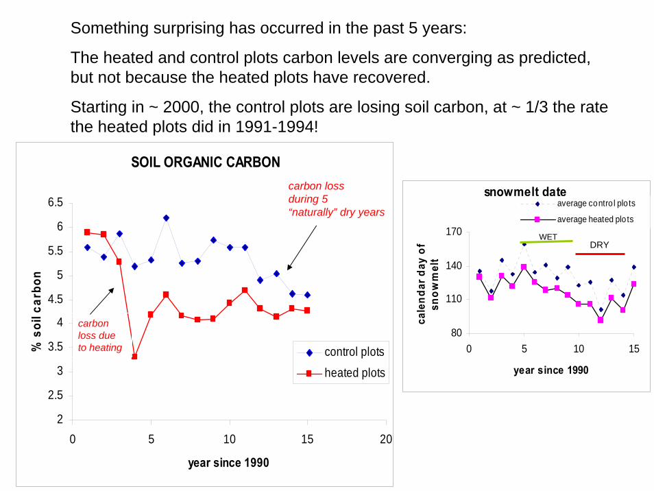
Something surprising has occurred in the past 5 years:
The heated and control plots carbon levels are converging as predicted, but not because the heated plots have recovered.
Starting in ~ 2000, the control plots are losing soil carbon, at ~ 1/3 the rate the heated plots did in 1991-1994!
SOIL ORGANIC CARBON
2
2.5
3
3.5
4
4.5
5
5.5
6
6.5
0 5 10 15 20
year since 1990
% s
oil c
arbo
n
control plots
heated plots
carbon loss during 5 “naturally” dry years
carbon loss due to heating
snowmelt date
80
110
140
170
0 5 10 15
year since 1990
cale
ndar
day
of
snow
mel
t
average contro l plo ts
average heated plots
DRYWET

AGB in the control plots in 1999-2004
resembles
AGB in the heated plots in 1993-1997
Thus soil carbon in the control plots in 99-04 behaved like soil carbon in the heated plots in 93-97
Our model suggests that plant community composition/productivity controls soil carbon;
Above-Ground Biomass (AGB) of forbs and shrubs drives the model.

Effect on Carbon
turnover
Response to Climate
Medium lignin:N
Lower lignin:N
Shallow rooted(sensitive to drought)
Forb:Erigeron
speciosus
Forb:Delphinium nuttallianum
Deep rooted(less sensitive to drought)
Forb:Ligusticum
porteri
Forb:Helianthella
quinquinervis
Species matter! Response to climate vs. effect on soil carbon turnover

What is a sensible set of plant traits/categories?
Albedo
Contribution to NPP and thus carbon input to soil
Lignin:N of foliage
Sensitivity to climate change (e.g., rooting depth)
Transpiration rate
LAI or Shading of soil beneath plant
Canopy roughness
Categories: for each we might consider 3 levels: high, medium, low
Thus have 36 = 729 plant categories.Just based on on the RMBL experience: the first 4 above or 34 = 81
The warming meadow contains about 75 plant species!

The feedback linkages in the meadow are very complex.
Yet we have not even begun here to look at:
•Other Habitats (tundra, desert, savannah, temperate forests, boreal forests, tropics, freshwater, marine …)
•Larger Spatial Scales (emergent phenomena?)
•Animals (grazers, pollinators, …)
•Other Climate Characteristics (extreme events, …)
•Carbon Dioxide increase (water efficiency, growth stimulation)
•Nitrogen Deposition (N addition can increase carbon storage)
•Land Use Changes (albedo, water exchange …)
•Invasive Species (carbon storage, albedo, water exchange)
•Genetic differences (influences shifts in community composition) between populations

Summary•Analysis of the long-term climate record suggests that strong positive feedback operates in Earth’s climate system.
•An ecosystem warming experiment provides further evidence for mechanisms that induce strong feedback responses.
•Current climate models do not incorporate these feedback effects and therefore are likely to be underestimating the magnitude of future warming.
•Developing a global-scale understanding of the sign and strength of these feedbacks is a huge challenge.


