
GROTHENDIECK-TYPE INEQUALITIESIN COMBINATORIAL OPTIMIZATION
SUBHASH KHOT AND ASSAF NAOR
Abstract. We survey connections of the Grothendieck inequality and its variants to com-binatorial optimization and computational complexity.
Contents
1. Introduction 21.1. Assumptions from computational complexity 31.2. Convex and semidefinite programming 42. Applications of the classical Grothendieck inequality 52.1. Cut norm estimation 52.1.1. Szemeredi partitions 82.1.2. Frieze-Kannan matrix decomposition 102.1.3. Maximum acyclic subgraph 112.1.4. Linear equations modulo 2 142.2. Rounding 163. The Grothendieck constant of a graph 183.1. Algorithmic consequences 203.1.1. Spin glasses 203.1.2. Correlation clustering 204. Kernel clustering and the propeller conjecture 215. The Lp Grothendieck problem 256. Higher rank Grothendieck inequalities 287. Hardness of approximation 29References 31
S. K. was partially supported by NSF CAREER grant CCF-0833228, NSF Expeditions grant CCF-0832795, an NSF Waterman award, and BSF grant 2008059. A. N. was partially supported by NSF Expe-ditions grant CCF-0832795, BSF grant 2006009, and the Packard Foundation.
1
1. Introduction
The Grothendieck inequality asserts that there exists a universal constant K ∈ (0,∞)such that for every m,n ∈ N and every m× n matrix A = (aij) with real entries we have
max
m∑i=1
n∑j=1
aij〈xi, yj〉 : ximi=1, yjnj=1 ⊆ Sn+m−1
6 K max
m∑i=1
n∑j=1
aijεiδj : εimi=1, δjnj=1 ⊆ −1, 1
. (1)
Here, and in what follows, the standard scalar product on Rk is denoted 〈x, y〉 =∑k
i=1 xiyiand the Euclidean sphere in Rk is denoted Sk−1 = x ∈ Rk :
∑ki=1 x
2i = 1. We refer
to [34, 56] for the simplest known proofs of the Grothendieck inequality; see Section 2.2 fora proof of (1) yielding the best known bound on K. Grothendieck proved the inequality (1)in [45], though it was stated there in a different, but equivalent, form. The formulation ofthe Grothendieck inequality appearing in (1) is due to Lindenstrauss and Pe lczynski [83].
The Grothendieck inequality is of major importance to several areas, ranging from Banachspace theory to C∗ algebras and quantum information theory. We will not attempt to indicatehere this wide range of applications of (1), and refer instead to [83, 114, 100, 55, 37, 34, 19, 1,40, 33, 102, 101] and the references therein. The purpose of this survey is to focus solely onapplications of the Grothendieck inequality and its variants to combinatorial optimization,and to explain their connections to computational complexity.
The infimum over those K ∈ (0,∞) for which (1) holds for all m,n ∈ N and all m × nmatrices A = (aij) is called the Grothendieck constant, and is denoted KG. Evaluating theexact value of KG remains a long-standing open problem, posed by Grothendieck in [45].In fact, even the second digit of KG is currently unknown, though clearly this is of lesserimportance than the issue of understanding the structure of matrices A and spherical config-urations ximi=1, yjnj=1 ⊆ Sn+m−1 which make the inequality (1) “most difficult”. Followinga series of investigations [45, 83, 107, 77, 78], the best known upper bound [21] on KG is
KG <π
2 log(1 +√
2) = 1.782..., (2)
and the best known lower bound [105] on KG is
KG >π
2eη
20 = 1.676..., (3)
where η0 = 0.25573... is the unique solution of the equation
1− 2
√2
π
∫ η
0
e−z2/2dz =
2
πe−η
2
.
In [104] the problem of estimating KG up to an additive error of ε ∈ (0, 1) was reduced to anoptimization over a compact space, and by exhaustive search over an appropriate net it wasshown that there exists an algorithm that computes KG up to an additive error of ε ∈ (0, 1)in time exp(exp(O(1/ε3))). It does not seem likely that this approach can yield computerassisted proofs of estimates such as (2) and (3), though to the best of our knowledge thishas not been attempted.
2
In the above discussion we focused on the classical Grothendieck inequality (1). However,the literature contains several variants and extensions of (1) that have been introduced forvarious purposes and applications in the decades following Grothendieck’s original work.In this survey we describe some of these variants, emphasizing relatively recent develop-ments that yielded Grothendieck-type inequalities that are a useful tool in the design ofpolynomial time algorithms for computing approximate solutions of computationally hardoptimization problems. In doing so, we omit some important topics, including applicationsof the Grothendieck inequality to communication complexity and quantum information the-ory. While these research directions can be viewed as dealing with a type of optimizationproblem, they are of a different nature than the applications described here, which belong toclassical optimization theory. Connections to communication complexity have already beencovered in the survey of Lee and Shraibman [81]; we refer in addition to [84, 80, 85, 86]for more information on this topic. An explanation of the relation of the Grothendieckinequality to quantum mechanics is contained in Section 19 of Pisier’s survey [101], thepioneering work in this direction being that of Tsirelson [114]. An investigation of thesequestions from a computational complexity point of view was initiated in [28], where it wasshown, for example, how to obtain a polynomial time algorithm for computing the entan-gled value of an XOR game based on Tsirelson’s work. We hope that the developmentssurrounding applications of the Grothendieck inequality in quantum information theory willeventually be surveyed separately by experts in this area. Interested readers are referredto [114, 37, 28, 1, 54, 98, 102, 61, 22, 80, 86, 106, 101]. Perhaps the most influential variantsof the Grothendieck inequality are its noncommutative generalizations. The noncommuta-tive versions in [99, 49] were conjectured by Grothendieck himself [45]; additional extensionsto operator spaces are extensively discussed in Pisier’s survey [101]. We will not describethese developments here, even though we believe that they might have applications to op-timization theory. Finally, multi-linear extensions of the Grothendieck inequality have alsobeen investigated in the literature; see for example [115, 112, 20, 109] and especially Blei’sbook [19]. We will not cover this research direction since its relation to classical combinato-rial optimization has not (yet?) been established, though there are recent investigations ofmulti-linear Grothendieck inequalities in the context of quantum information theory [98, 80].
Being a mainstay of functional analysis, the Grothendieck inequality might attract tothis survey readers who are not familiar with approximation algorithms and computationalcomplexity. We wish to encourage such readers to persist beyond this introduction so thatthey will be exposed to, and hopefully eventually contribute to, the use of analytic tools incombinatorial optimization. For this reason we include Sections 1.1, 1.2 below; two very basicintroductory sections intended to quickly provide background on computational complexityand convex programming for non-experts.
1.1. Assumptions from computational complexity. At present there are few uncondi-tional results on the limitations of polynomial time computation. The standard practice inthis field is to frame an impossibility result in computational complexity by asserting thatthe polynomial time solvability of a certain algorithmic task would contradict a benchmarkhypothesis. We briefly describe below two key hypotheses of this type.
A graph G = (V,E) is 3-colorable if there exists a partition C1, C2, C3 of V such thatfor every i ∈ 1, 2, 3 and u, v ∈ Ci we have u, v /∈ E. The P 6= NP hypothesis as-serts that there is no polynomial time algorithm that takes an n-vertex graph as input and
3
determines whether or not it is 3-colorable. We are doing an injustice to this importantquestion by stating it this way, since it has many far-reaching equivalent formulations. Werefer to [39, 108, 31] for more information, but for non-experts it suffices to keep the abovesimple formulation in mind.
When we say that assuming P 6= NP no polynomial time algorithm can perform a certaintask T (e.g., evaluating the maximum of a certain function up to a predetermined error) wemean that given an algorithm ALG that performs the task T one can design an algorithmALG′ that determines whether or not any input graph is 3-colorable while making at mostpolynomially many calls to the algorithm ALG, with at most polynomially many additionalTuring machine steps. Thus, if ALG were a polynomial time algorithm then the same wouldbe true for ALG′, contradicting the P 6= NP hypothesis. Such results are called hardnessresults. The message that non-experts should keep in mind is that a hardness result isnothing more than the design of a new algorithm for 3-colorability, and if one accepts theP 6= NP hypothesis then it implies that there must exist inputs on which ALG takes super-polynomial time to terminate.
The Unique Games Conjecture (UGC) asserts that for every ε ∈ (0, 1) there exists a primep = p(ε) ∈ N such that no polynomial time algorithm can perform the following task. Theinput is a system of m linear equations in n variables x1, . . . , xn, each of which has the formxi − xj ≡ cij mod p (thus the input is S ⊆ 1, . . . , n × 1, . . . , n and cij(i,j)∈S ⊆ N).The algorithm must determine whether there exists an assignment of an integer value toeach variable xi such that at least (1 − ε)m of the equations are satisfied, or whether noassignment of such values can satisfy more than εm of the equations. If neither of thesepossibilities occur, then an arbitrary output is allowed.
As in the case of P 6= NP , saying that assuming the UGC no polynomial time algorithmcan perform a certain task T is the same as designing a polynomial time algorithm thatsolves the above linear equations problem while making at most polynomially many calls toa “black box” that can perform the task T . The UGC was introduced in [62], though theabove formulation of it, which is equivalent to the original one, is due to [64]. The use ofthe UGC as a hardness hypothesis has become popular over the past decade; we refer to thesurvey [63] for more information on this topic.
To simplify matters (while describing all the essential ideas), we allow polynomial timealgorithms to be randomized. Most (if not all) of the algorithms described here can be turnedinto deterministic algorithms, and corresponding hardness results can be stated equally wellin the context randomized or deterministic algorithms. We will ignore these distinctions,even though they are important. Moreover, it is widely believed that in our context thesedistinctions do not exist, i.e., randomness does not add computational power to polynomialtime algorithms; see for example the discussion of the NP 6⊆ BPP hypothesis in [11].
1.2. Convex and semidefinite programming. An important paradigm of optimizationtheory is that one can efficiently optimize linear functionals over compact convex sets thathave a “membership oracle”. A detailed exposition of this statement is contained in [46],but for the sake of completeness we now quote the precise formulation of the results thatwill be used in this article.
Let K ⊆ Rn be a compact convex set. We are also given a point z ∈ Qn and two radiir, R ∈ (0,∞)∩Q such that B(z, r) ⊆ K ⊆ B(z, R), where B(z, t) = x ∈ Rn : ‖x−z‖2 6 t.In what follows, stating that an algorithm is polynomial means that we allow the running time
4
to grow at most polynomially in the number of bits required to represent the data (z, r, R).Thus, if, say, z = 0, r = 2−n and R = 2n then the running time will be polynomial in thedimension n. Assume that there exists an algorithm ALG with the following properties. Theinput of ALG is a vector y ∈ Qn and ε ∈ (0, 1)∩Q. The running time of ALG is polynomialin n and the number of bits required to represent the data (ε, y). The output of ALG is theassertion that either the distance of y from K is at most ε, or that the distance of y fromthe complement of K is at most ε. Then there exists an algorithm ALG′ that takes as inputa vector c = (c1, . . . , cn) ∈ Qn and ε ∈ (0, 1) ∩Q and outputs a vector y = (y1, . . . , yn) ∈ Rn
that is at distance at most ε from K and for every x = (x1, . . . , xn) ∈ K that is at distancegreater than ε from the complement of K we have
∑ni=1 ciyi >
∑ni=1 cixi − ε. The running
time of ALG′ is allowed to grow at most polynomially in n and the number of bits requiredto represent the data (z, r, R, c, ε). This important result is due to [57]; we refer to [46] foran excellent account of this theory.
The above statement is a key tool in optimization, as it yields a polynomial time methodto compute the maximum of linear functionals on a given convex body with arbitrarilygood precision. We note the following special case of this method, known as semidefiniteprogramming. Assume that n = k2 and think of Rn as the space of all k×k matrices. Assumethat we are given a compact convex setK ⊆ Rn that satisfies the above assumptions, and thatfor a given k×k matrix (cij) we wish to compute in polynomial time (up to a specified additive
error) the maximum of∑k
i=1
∑kj=1 cijxij over the set of symmetric positive semidefinite
matrices (xij) that belong to K. This can indeed be done, since determining whether a givensymmetric matrix is (approximately) positive semidefinite is an eignevalue computation andhence can be performed in polynomial time. The use of semidefinite programming to designapproximation algorithms is by now a deep theory of fundamental importance to severalareas of theoretical computer science. The Goemans-Williamson MAX-CUT algorithm [42]was a key breakthrough in this context. It is safe to say that after the discovery of thisalgorithm the field of approximation algorithms was transformed, and many subsequentresults, including those presented in the present article, can be described as attempts tomimic the success of the Goemans-Williamson approach in other contexts.
2. Applications of the classical Grothendieck inequality
The classical Grothendieck inequality (1) has applications to algorithmic questions ofcentral interest. These applications will be described here in some detail. In Section 2.1 wediscuss the cut norm estimation problem, whose relation to the Grothendieck inequality wasfirst noted in [8]. This is a generic combinatorial optimization problem that contains well-studied questions as subproblems. Examples of its usefulness are presented in Sections 2.1.1,2.1.2, 2.1.3, 2.1.4. Section 2.2 is devoted to the rounding problem, including the (algorithmic)method behind the proof of the best known upper bound on the Grothendieck constant.
2.1. Cut norm estimation. Let A = (aij) be an m× n matrix with real entries. The cutnorm of A is defined as follows
‖A‖cut = maxS⊆1,...,mT⊆1,...,n
∣∣∣∣∣∣∣∑i∈Sj∈T
aij
∣∣∣∣∣∣∣ . (4)
5
We will now explain how the Grothendieck inequality can be used to obtain a polynomialtime algorithm for the following problem. The input is an m× n matrix A = (aij) with realentries, and the goal of the algorithm is to output in polynomial time a number α that isguaranteed to satisfy
‖A‖cut 6 α 6 C‖A‖cut, (5)
where C is a (hopefully not too large) universal constant. A closely related algorithmic goalis to output in polynomial time two subsets S0 ⊆ 1, . . . ,m and T0 ⊆ 1, . . . , n satisfying∣∣∣∣∣∣∣
∑i∈S0j∈T0
aij
∣∣∣∣∣∣∣ >1
C‖A‖cut. (6)
The link to the Grothendieck inequality is made via two simple transformations. Firstly,define an (m+ 1)× (n+ 1) matrix B = (bij) as follows.
B =
a11 a12 . . . a1n −
∑nk=1 a1k
a21 a22 . . . a2n −∑n
k=1 a2k...
.... . .
......
am1 am2 . . . amn −∑n
k=1 amk−∑m
`=1 a`1 −∑m
`=1 a`2 . . . −∑m
`=1 a`n∑n
k=1
∑m`=1 a`k
. (7)
Observe that‖A‖cut = ‖B‖cut. (8)
Indeed, for every S ⊆ 1, . . . ,m + 1 and T ⊆ 1, . . . , n + 1 define S∗ ⊆ 1, . . . ,m andT ∗ ⊆ 1, . . . , n by
S∗ =
S if m+ 1 /∈ S,1, . . . ,mr S if m+ 1 ∈ S, and T ∗ =
T if n+ 1 /∈ T,1, . . . , nr T if n+ 1 ∈ T.
One checks that for all S ⊆ 1, . . . ,m+ 1 and T ⊆ 1, . . . , n+ 1 we have∣∣∣∣∣∣∣∑i∈Sj∈T
bij
∣∣∣∣∣∣∣ =
∣∣∣∣∣∣∣∑i∈S∗j∈T ∗
aij
∣∣∣∣∣∣∣ ,implying (8). We next claim that
‖B‖cut =1
4‖B‖∞→1, (9)
where
‖B‖∞→1 = max
m+1∑i=1
n+1∑j=1
bijεiδj : εim+1i=1 , δjn+1
j=1 ⊆ −1, 1
. (10)
To explain this notation observe that ‖B‖∞→1 is the norm of B when viewed as a linearoperator from `n∞ to `m1 . Here, and in what follows, for p ∈ [1,∞] and k ∈ N the space `kpis Rk equipped with the `p norm ‖ · ‖p, where ‖x‖pp =
∑k`=1 |x`|p for x = (x1, . . . , xk) ∈ Rk
(for p =∞ we set as usual ‖x‖∞ = maxi∈1,...,n |xi|). Though it is important, this operatortheoretic interpretation of the quantity ‖B‖∞→1 will not have any role in this survey, so itmay be harmlessly ignored at first reading.
6
The proof of (9) is simple: for εim+1i=1 , δjn+1
j=1 ⊆ −1, 1 define S+, S− ⊆ 1, . . . ,m+ 1and T+, T− ⊆ 1, . . . , n + 1 by setting S± = i ∈ 1, . . . ,m + 1 : εi = ±1 and T± =j ∈ 1, . . . , n+ 1 : δj = ±1. Then
m+1∑i=1
n+1∑j=1
bijεiδj =∑i∈S+
j∈T+
bij +∑i∈S−
j∈T−
bij −∑i∈S+
j∈T−
bij −∑i∈S−
j∈T+
bij 6 4‖B‖cut. (11)
This shows that ‖B‖∞→1 6 4‖B‖cut (for any matrix B, actually, not just the specific choicein (7); we will use this observation later, in Section 2.1.3). In the reverse direction, givenS ⊆ 1, . . . ,m+1 and T ⊆ 1, . . . , n+1 define for i ∈ 1, . . . ,m+1 and j ∈ 1, . . . , n+1,
εi =
1 if i ∈ S,−1 if i /∈ S, and δj =
1 if j ∈ T,−1 if j /∈ T.
Then, since the sum of each row and each column of B vanishes,∑i∈Sj∈T
bij =m+1∑i=1
n+1∑j=1
bij1 + εi
2· 1 + δj
2=
1
4
m+1∑i=1
n+1∑j=1
bijεiδj 61
4‖B‖∞→1.
This completes the proof of (9). We summarize the above simple transformations in thefollowing lemma.
Lemma 2.1. Let A = (aij) be an m × n matrix with real entries and let B = (bij) be the(m+ 1)× (n+ 1) matrix given in (7). Then
‖A‖cut =1
4‖B‖∞→1.
A consequence of Lemma 2.1 is that the problem of approximating ‖A‖cut in polynomialtime is equivalent to the problem of approximating ‖A‖∞→1 in polynomial time in the sensethat any algorithm for one of these problems can be used to obtain an algorithm for the otherproblem with the same running time (up to constant factors) and the same (multiplicative)approximation guarantee.
Given an m× n matrix A = (aij) consider the following quantity.
SDP(A) = max
m∑i=1
n∑j=1
aij〈xi, yj〉 : ximi=1, yjnj=1 ⊆ Sn+m−1
. (12)
The maximization problem in (12) falls into the framework of semidefinite programmingas discussed in Section 1.2. Therefore SDP(A) can be computed in polynomial time witharbitrarily good precision. It is clear that SDP(A) > ‖A‖∞→1, because the maximum in (12)is over a bigger set than the maximum in (10). The Grothendieck inequality says thatSDP(A) 6 KG‖A‖∞→1, so we have
‖A‖∞→1 6 SDP(A) 6 KG‖A‖∞→1.
Thus, the polynomial time algorithm that outputs the number SDP(A) is guaranteed to bewithin a factor of KG of ‖A‖∞→1. By Lemma 2.1, the algorithm that outputs the numberα = 1
4SDP(B), where the matrix B is as in (7), satisfies (5) with C = KG.
Section 7 is devoted to algorithmic impossibility results. But, it is worthwhile to makeat this juncture two comments regarding hardness of approximation. First of all, unless
7
P = NP , we need to introduce an error C > 1 in our requirement (5). This was observedin [8]: the classical MAXCUT problem from algorithmic graph theory was shown in [8] tobe a special case of the problem of computing ‖A‖cut, and therefore by [51] we know thatunless P = NP there does not exist a polynomial time algorithm that outputs a number αsatisfying (5) with C strictly smaller than 17
16. In fact, by a reduction to the MAX DICUT
problem one can show that C must be at least 1312
, unless P = NP ; we refer to Section 7and [8] for more information on this topic.
Another (more striking) algorithmic impossibility result is based on the Unique GamesConjecture (UGC). Clearly the above algorithm cannot yield an approximation guaranteestrictly smaller than KG (this is the definition of KG). In fact, it was shown in [104] thatunless the UGC is false, for every ε ∈ (0, 1) any polynomial time algorithm for estimating‖A‖cut whatsoever, and not only the specific algorithm described above, must make anerror of at least KG − ε on some input matrix A. Thus, if we assume the UGC then theclassical Grothendieck constant has a complexity theoretic interpretation: it equals the bestapproximation ratio of polynomial time algorithms for the cut norm problem. Note that [104]manages to prove this statement despite the fact that the value of KG is unknown.
We have thus far ignored the issue of finding in polynomial time the subsets S0, T0
satisfying (6), i.e., we only explained how the Grothendieck inequality can be used forpolynomial time estimation of the quantity ‖A‖cut without actually finding efficiently sub-sets at which ‖A‖cut is approximately attained. In order to do this we cannot use theGrothendieck inequality as a black box: we need to look into its proof and argue that ityields a polynomial time procedure that converts vectors ximi=1, yjnj=1 ⊆ Sn+m−1 intosigns εimi=1, δjnj=1 ⊆ −1, 1 (this is known as a rounding procedure). It is indeed pos-sible to do so, as explained in Section 2.2. We postpone the explanation of the roundingprocedure that hides behind the Grothendieck inequality in order to first give examples whyone might want to efficiently compute the cut norm of a matrix.
2.1.1. Szemeredi partitions. The Szemeredi regularity lemma [111] (see also [72]) is a generaland very useful structure theorem for graphs, asserting (informally) that any graph can bepartitioned into a controlled number of pieces that interact with each other in a pseudo-random way. The Grothendieck inequality, via the cut norm estimation algorithm, yields apolynomial time algorithm that, when given a graph G = (V,E) as input, outputs a partitionof V that satisfies the conclusion of the Szemeredi regularity lemma.
To make the above statements formal, we need to recall some definitions. Let G = (V,E)be a graph. For every disjoint X, Y ⊆ V denote the number of edges joining X and Y bye(X, Y ) = |(u, v) ∈ X × Y : u, v ∈ E|. Let X, Y ⊆ V be disjoint and nonempty, andfix ε, δ ∈ (0, 1). The pair of vertex sets (X, Y ) is called (ε, δ)-regular if for every S ⊆ X and
T ⊆ Y that are not too small, the quantity e(S,T )|S|·|T | (the density of edges between S and T ) is
essentially independent of the pair (S, T ) itself. Formally, we require that for every S ⊆ Xwith |S| > δ|X| and every T ⊆ Y with |T | > δ|Y | we have
∣∣∣∣ e(S, T )
|S| · |T |− e(X, Y )
|X| · |Y |
∣∣∣∣ 6 ε. (13)
8
The almost uniformity of the numbers e(S,T )|S|·|T | as exhibited in (13) says that the pair (X, Y ) is
“pseudo-random”, i.e., it is similar to a random bipartite graph where each (x, y) ∈ X × Yis joined by an edge independently with probability e(X,Y )
|X|·|Y | .
The Szemeredi regularity lemma says that for all ε, δ, η ∈ (0, 1) and k ∈ N there existsK = K(ε, δ, η, k) ∈ N such that for all n ∈ N any n-vertex graph G = (V,E) can bepartitioned into m-sets S1, . . . , Sm ⊆ V with the following properties
• k 6 m 6 K,• |Si| − |Sj| 6 1 for all i, j ∈ 1, . . . ,m,• the number of i, j ∈ 1, . . . ,m with i < j such that the pair (Si, Sj) is (ε, δ)-regular
is at least (1− η)(m2
).
Thus every graph is almost a superposition of a bounded number of pseudo-random graphs,the key point being that K is independent of n and the specific combinatorial structure ofthe graph in question.
It would be of interest to have a way to produce a Szemeredi partition in polynomial timewith K independent of n (this is a good example of an approximation algorithm: one mightcare to find such a partition into the minimum possible number of pieces, but producing anypartition into boundedly many pieces is already a significant achievement). Such a polyno-mial time algorithm was designed in [5] (see also [73]). We refer to [5, 73] for applicationsof algorithms for constructing Szemeredi partitions, and to [5] for a discussion of the com-putational complexity of this algorithmic task. We shall now explain how the Grothendieckinequality yields a different approach to this problem, which has some advantages over [5, 73]that will be described later. The argument below is due to [8].
Assume that X, Y are disjoint n-point subsets of a graph G = (V,E). How can we deter-mine in polynomial time whether or not the pair (X, Y ) is close to being (ε, δ)-regular? Itturns out that this is the main “bottleneck” towards our goal to construct Szemeredi parti-tions in polynomial time. To this end consider the following n×n matrix A = (axy)(x,y)∈X×Y .
axy =
1− e(X,Y )
|X|·|Y | if x, y ∈ E,− e(X,Y )|X|·|Y | if x, y /∈ E.
(14)
By the definition of A, if S ⊆ X and T ⊆ Y then∣∣∣∣∣∣∣∑x∈Sy∈T
axy
∣∣∣∣∣∣∣ = |S| · |T | ·∣∣∣∣ e(S, T )
|S| · |T |− e(X, Y )
|X| · |Y |
∣∣∣∣ . (15)
Hence if (X, Y ) is not (ε, δ)-regular then ‖A‖cut > εδ2n2. The approximate cut norm al-gorithm based on the Grothendieck inequality, together with the rounding procedure inSection 2.2, finds in polynomial time subsets S ⊆ X and T ⊆ Y such that
min
n|S|, n|T |, n2
∣∣∣∣ e(S, T )
|S| · |T |− e(X, Y )
|X| · |Y |
∣∣∣∣ (15)
>
∣∣∣∣∣∣∣∑x∈Sy∈T
axy
∣∣∣∣∣∣∣ >1
KG
εδ2n2 >1
2εδ2n2.
This establishes the following lemma.
9
Lemma 2.2. There exists a polynomial time algorithm that takes as input two disjoint n-point subsets X, Y of a graph, and either decides that (X, Y ) is (ε, δ)-regular or finds S ⊆ Xand T ⊆ Y with
|S|, |T | > 1
2εδ2n and
∣∣∣∣ e(S, T )
|S| · |T |− e(X, Y )
|X| · |Y |
∣∣∣∣ > 1
2εδ2.
From Lemma 2.2 it is quite simple to design a polynomial algorithm that constructs aSzemeredi partition with bounded cardinality; compare Lemma 2.2 to Corollary 3.3 in [5]and Theorem 1.5 in [73]. We will not explain this deduction here since it is identical tothe argument in [5]. We note that the quantitative bounds in Lemma 2.2 improve over thecorresponding bounds in [5, 73] yielding, say, when ε = δ = η, an algorithm with the bestknown bound on K as a function of ε (this bound is nevertheless still huge, as must be thecase due to [44]; see also [30]). See [8] for a precise statement of these bounds. In addition,the algorithms of [5, 73] worked only in the “dense case”, i.e., when ‖A‖cut, for A as in (14),is of order n2, while the above algorithm does not have this requirement. This observationcan be used to design the only known polynomial time algorithm for sparse versions of theSzemeredi regularity lemma [4] (see also [41]). We will not discuss the sparse version of theregularity lemma here, and refer instead to [71, 72] for a discussion of this topic. We alsorefer to [4] for additional applications of the Grothendieck inequality in sparse settings.
2.1.2. Frieze-Kannan matrix decomposition. The cut norm estimation problem was origi-nally raised in the work of Frieze and Kannan [38] which introduced a method to designpolynomial time approximation schemes for dense constraint satisfaction problems. The keytool for this purpose is a decomposition theorem for matrices that we now describe.
An m × n matrix D = (dij) is called a cut matrix if there exist subsets S ⊆ 1, . . . ,mand T ⊆ 1, . . . , n, and d ∈ R such that for all (i, j) ∈ 1, . . . ,m × 1, . . . , n we have,
dij =
d if (i, j) ∈ S × T,0 if (i, j) /∈ S × T. (16)
Denote the matrix D defined in (16) by CUT (S, T, d). In [38] it is proved that for everyε > 0 there exists an integer s = O(1/ε2) such that for any m × n matrix A = (aij) withentries bounded in absolute value by 1, there are cut matrices D1, . . . , Ds satisfying∥∥∥∥∥A−
s∑k=1
Dk
∥∥∥∥∥cut
6 εmn. (17)
Moreover, these cut matrices D1, . . . , Ds can be found in time C(ε)(mn)O(1). We shall nowexplain how this is done using the cut norm approximation algorithm of Section 2.1.
The argument is iterative. Set A0 = A, and assuming that the cut matrices D1, . . . , Dr
have already been defined write Ar = (aij(r)) = A−∑r
k=1Dk. We are done if ‖Ar‖cut 6 εmn,so we may assume that ‖Ar‖cut > εmn. By the cut norm approximation algorithm we canfind in polynomial time S ⊆ 1, . . . ,m and T ⊆ 1, . . . , n satisfying∣∣∣∣∣∣∣
∑i∈Sj∈T
aij(r)
∣∣∣∣∣∣∣ > c‖Ar‖cut > cεmn, (18)
10
where c > 0 is a universal constant. Set
d =1
|S| · |T |∑i∈Sj∈T
aij(r).
Define Dr+1 = CUT (S, T, d) and Ar+1 = (aij(r + 1)) = Ar −Dr+1. Then by expanding thesquares we have,
m∑i=1
n∑j=1
aij(r + 1)2 =m∑i=1
n∑j=1
aij(r)2 − 1
|S| · |T |
∑i∈Sj∈T
aij(r)
2
(18)
6m∑i=1
n∑j=1
aij(r)2 − c2ε2mn.
It follows inductively that if we can carry out this procedure r times then
0 6m∑i=1
n∑j=1
aij(r)2 6
m∑i=1
n∑j=1
a2ij − rc2ε2mn 6 mn− rc2ε2mn,
where we used the assumption that |aij| 6 1. Therefore the above iteration must terminateafter d1/(c2ε2)e steps, yielding (17). We note that the bound s = O(1/ε2) in (17) cannot beimproved [6]; see also [89, 30] for related lower bounds.
The key step in the above algorithm was finding sets S, T as in (18). In [38] an algorithmwas designed that, given an m × n matrix A = (aij) and ε > 0 as input, produces in time
21/εO(1)(mn)O(1) subsets S ⊆ 1, . . . ,m and T ⊆ 1, . . . , n satisfying∣∣∣∣∣∣∣
∑i∈Sj∈T
aij
∣∣∣∣∣∣∣ > ‖A‖cut − εmn. (19)
The additive approximation guarantee in (19) implies (18) only if ‖A‖cut > ε(c+ 1)mn, andsimilarly the running time is not polynomial if, say, ε = n−Ω(1). Thus the Kannan-Friezemethod is relevant only to “dense” instances, while the cut norm algorithm based on theGrothendieck inequality applies equally well for all values of ‖A‖cut. This fact, combinedwith more work (and, necessarily, additional assumptions on the matrix A), was used in [29]to obtain a sparse version of (17): with εmn in the right hand side of (17) replaced byε‖A‖cut and s = O(1/ε2) (importantly, here s is independent of m,n).
We have indicated above how the cut norm approximation problem is relevant to Kannan-Frieze matrix decompositions, but we did not indicate the uses of such decompositions sincethis is beyond the scope of the current survey. We refer to [38, 6, 15, 29] for a variety ofapplications of this methodology to combinatorial optimization problems.
2.1.3. Maximum acyclic subgraph. In the maximum acyclic subgraph problem we are givenas input an n-vertex directed graph G = (1, . . . , n, E). Thus E consists of a family ofordered pairs of distinct elements in 1, . . . , n. We are interested in the maximum of∣∣(i, j) ∈ 1, . . . , n2 : σ(i) < σ(j) ∩ E
∣∣− ∣∣(i, j) ∈ 1, . . . , n2 : σ(i) > σ(j) ∩ E∣∣
over all possible permutations σ ∈ Sn (Sn denotes the group of permutations of 1, . . . , n).In words, the quantity of interest is the maximum over all orderings of the vertices of thenumber of edges going “forward” minus the number of edges going “backward”. Note that itis trivial to get at least half of the edges to go forward by considering a random permutation,
11
so in essence we are measuring here the advantage of the best possible ordering over a randomordering. The best known approximation algorithm for this problem was discovered in [26]as an application of the cut norm approximation algorithm.
It is most natural to explain the algorithm of [26] for a weighted version of the maximumacyclic subgraph problem. Let W : 1, . . . , n × 1, . . . , n → R be skew symmetric, i.e.,W (u, v) = −W (v, u) for all u, v ∈ 1, . . . , n. For σ ∈ Sn define
W (σ) =∑
u,v∈1,...,nu<v
W (σ(u), σ(v)).
Thus W (σ) is the sum of the entries of W that lie above the diagonal after the rows andcolumns of W have been permuted according to the permutation σ. We are interested in thequantity MW = maxσ∈SnW (σ). The case of a directed graph G = (1, . . . , n, E) describedabove corresponds to the matrix W (u, v) = 1(u,v)∈E − 1(v,u)∈E.
Theorem 2.3 ([26]). The exists a polynomial time algorithm that takes as input an n×n skewsymmetric W : 1, . . . , n × 1, . . . , n → R and outputs a permutation σ ∈ Sn satisfying1
W (σ) &MW
log n.
Proof. The proof below is a slight variant of the reasoning of [26]. By the cut norm approx-imation algorithm one can find in polynomial time two subsets S, T ⊆ 1, . . . , n satisfying∑
u∈Sv∈T
W (u, v) > c‖W‖cut, (20)
where c ∈ (0,∞) is a universal constant. Note that we do not need to take the absolutevalue of the left hand side of (20) because W is skew symmetric. Observe also that since Wis skew symmetric we have
∑u,v∈S∩T W (u, v) = 0 and therefore∑
u∈Sv∈T
W (u, v) =∑
u∈SrTv∈TrS
W (u, v) +∑
u∈SrTv∈S∩T
W (u, v) +∑u∈S∩Tv∈TrS
W (u, v).
By replacing the pair of subsets (S, T ) by one of (SrT, TrS), (SrT, S∩T ), (S∩T, TrS),and replacing the constant c is (20) by c/3, we may assume without loss of generality that (20)holds with S and T disjoint. Denote R = 1, . . . , nr (S ∪ T ) and write S = s1, . . . , s|S|,T = t1, . . . , t|T | and R = r1, . . . , r|R|, where s1 < · · · < s|S|, t1 < · · · < t|T | andr1 < · · · < r|R|.
Define two permutations σ1, σ2 ∈ Sn as follows.
σ1(u) =
su if u ∈ 1, . . . , |S|,tu−|S| if u ∈ |S|+ 1, . . . , |S|+ |T |,ru−|S|−|T | if u ∈ |S|+ |T |+ 1, . . . , n,
and
σ2(u) =
r|R|−u+1 if u ∈ 1, . . . , |R|,s|R|+|S|−u+1 if u ∈ |R|+ 1, . . . , |R|+ |S|,tn−u+1 if u ∈ |R|+ |S|+ 1, . . . , n.
1Here, and in what follows, the relations &,. indicate the corresponding inequalities up to an absolutefactor. The relation stands for & ∧ ..
12
In words, σ1 orders 1, . . . , n by starting with the elements of S in increasing order, then theelements of T in increasing order, and finally the elements of R in increasing order. At thesame time, σ2 orders 1, . . . , n by starting with the elements of R in decreasing order, thenthe elements of S in decreasing order, and finally the elements of T in decreasing order. Thequantity W (σ1)+W (σ2) consists of a sum of terms of the form W (u, v) for u, v ∈ 1, . . . , n,where if (u, v) ∈ (S×S)∪ (T ×T )∪ (R×1, . . . , n) then both W (u, v) and W (v, u) appearexactly once in this sum, and if (u, v) ∈ S × T then W (u, v) appears twice in this sumand W (v, u) does not appear in this sum at all. Therefore, using the fact that W is skewsymmetric we have the following identity.
W (σ1) +W (σ2) = 2∑u∈Sv∈T
W (u, v).
It follows that for some ` ∈ 1, 2 we have
M(σ`) >∑u∈Sv∈T
W (u, v)(20)
> c‖W‖cut.
The output of the algorithm will be the permutation σ`, so it suffices to prove that
‖W‖cut &MW
log n. (21)
We will prove below that
‖W‖cut &1
log n
∑u,v∈1,...,n
u<v
W (u, v). (22)
Inequality (21) follows by applying (22) to W ′(u, v) = W (σ(u), σ(v)) for every σ ∈ Sn.To prove (22) first note that ‖W‖cut > 1
4‖W‖∞→1; we have already proved this inequality
as a consequence of the simple identity (11). Moreover, we have
‖W‖∞→1 & max
n∑u=1
n∑v=1
W (u, v) sin(αu − βv) : αunu=1, βvnv=1 ⊆ R
. (23)
Inequality (23) is a special case of (1) with the choice of vectors xu = (sinαu, cosαu) ∈ R2 andyv = (cos βv,− sin βv) ∈ R2. We note that this two-dimensional version of the Grothendieckinequality is trivial with the constant in the right hand side of (23) being 1
2, and it is shown
in [78] that the best constant in the right hand side of (23) is actually 1√2.
For every θ1, . . . , θn ∈ R, an application of (23) when αu = βu = θu and αu = βu = −θuyields the inequality
‖W‖cut &
∣∣∣∣∣n∑u=1
n∑v=1
W (u, v) sin (θu − θv)
∣∣∣∣∣ = 2
∣∣∣∣∣∣∣∑
u,v∈1,...,nu<v
W (u, v) sin (θu − θv)
∣∣∣∣∣∣∣ , (24)
13
where for the equality in (24) we used the fact that W is skew symmetric. Consequently, forevery k ∈ N we have
‖W‖cut &
∣∣∣∣∣∣∣∑
u,v∈1,...,nu<v
W (u, v) sin
(π(v − u)k
n
)∣∣∣∣∣∣∣ . (25)
By the standard orthogonality relation for the sine function, for every u, v ∈ 1, . . . , nsuch that u < v we have
2
n
n−1∑k=1
n−1∑`=1
sin
(π(v − u)k
n
)sin
(πk`
n
)= 1. (26)
Readers who are unfamiliar with (26) are referred to its derivation in the appendix of [26];it can be proved by substituting sin (π(v − u)k/n) = (eiπ(v−u)k/n − e−iπ(v−u)k/n)/(2i) andsin(πk`/n) = (eiπk`/n − e−iπk`/n)/(2i) into the left hand side of (26) and computing theresulting geometric sums explicitly. Now,∑
u,v∈1,...,nu<v
W (u, v)(26)=
2
n
∑u,v∈1,...,n
u<v
W (u, v)n−1∑k=1
n−1∑`=1
sin
(π(v − u)k
n
)sin
(πk`
n
)
62
n
n−1∑k=1
∣∣∣∣∣n−1∑`=1
sin
(πk`
n
)∣∣∣∣∣ ·∣∣∣∣∣∣∣∑
u,v∈1,...,nu<v
W (u, v) sin
(π(v − u)k
n
)∣∣∣∣∣∣∣(25)
.
∑n−1k=1
∣∣∑n−1`=1 sin
(πk`n
)∣∣n
‖W‖cut.
Hence, the desired inequality (22) will follow from∑n−1
k=1
∣∣∑n−1`=1 sin (πk`/n)
∣∣ . n log n. To
establish this estimate observe that by writing sin(πk`/n) = (eiπk`/n − e−iπk`/n)/(2i) andcomputing geometric sums explicitly, one sees that
∑n−1`=1 sin (πk`/n) = 0 if k is even and∑n−1
`=1 sin (πk`/n) = cot(πk/(2n)) if k is odd (see the appendix of [26] for the details of thiscomputation). Hence, since cot(θ) < 1/θ for every θ ∈ (0, π/2), we have
n−1∑k=1
∣∣∣∣∣n−1∑`=1
sin
(πk`
n
)∣∣∣∣∣ =
bn2−1c∑j=0
cot
(π(2j + 1)
2n
)6
2n
π
bn2−1c∑j=0
1
2j + 1. n log n
2.1.4. Linear equations modulo 2. Consider a system E of N linear equations modulo 2 inn Boolean variables z1, . . . , zn such that in each equation appear only three distinct vari-ables. Let MAXSAT(E) be the maximum number of equations in E that can be satisfiedsimultaneously. A random 0, 1 assignment of these variables satisfies in expectation N/2equations, so it is natural to ask for a polynomial time approximation algorithm to the quan-tity MAXSAT(E) − N/2. We describe below the best known [65] approximation algorithmfor this problem, which uses the Grothendieck inequality in a crucial way. The approxima-tion guarantee thus obtained is O(
√n/ log n). While this allows for a large error, it is shown
in [52] that for every ε ∈ (0, 1) if there were a polynomial time algorithm that approximates
MAXSAT(E)−N/2 to within a factor of 2(logn)1−ε in time 2(logn)O(1)then there would be an
14
algorithm for 3-colorability that runs in time 2(logn)O(1), a conclusion which is widely believed
to be impossible.Let E be a system of linear equations as described above. Write aijk = 1 if the equation
zi + zj + zk = 0 is in the system E . Similarly write aijk = −1 if the equation zi + zj + zk = 1is in E . Finally, write aijk = 0 if no equation in E corresponds to zi + zj + zk. Assume thatthe assignment (z1, . . . , zn) ∈ 0, 1n satisfies m of the equations in E . Then
n∑i=1
n∑j=1
n∑k=1
aijk(−1)zi+zj+zk = m− (N −m) = 2
(m− N
2
).
It follows that
max
n∑i=1
n∑j=1
n∑k=1
aijkεiεjεk : εini=1 ⊆ −1, 1
= 2
(MAXSAT(E)− N
2
)def= M. (27)
We will now present a randomized polynomial algorithm that outputs a number α ∈ Rwhich satisfies with probability at least 2
3,
1
20KG
√log n
nM 6 α 6M. (28)
Fix m ∈ N that will be determined later. Choose ε1, . . . , εm ∈ −1, 1n independently anduniformly at random and consider the following random variable.
α =1
10KG
max`∈1,...,m
max
n∑i=1
n∑j=1
n∑k=1
aijkε`i〈yj, zk〉 : yjnj=1, zknk=1 ⊆ S2n−1
. (29)
By the Grothendieck inequality we know that
α 61
10max
n∑i=1
n∑j=1
n∑k=1
aijkεiδjζk : εini=1, δjnj=1, ζknk=1 ⊆ −1, 1
6M. (30)
The final step in (30) follows from an elementary decoupling argument; see [65, Lem. 2.1].We claim that
Pr
[α >
1
20KG
√log n
nM
]> 1− e−cm/ 4√n. (31)
Once (31) is established, it would follow that for m 4√n we have α > 1
20KG
√lognnM with
probability at least 23. This combined with (30) would complete the proof of (28) since
α as defined in (29) can be computed in polynomial time, being the maximum of O ( 4√n)
semidefinite programs.To check (31) let ‖ · ‖ be the norm on Rn defined for every x = (x1, . . . , xn) ∈ Rn by
‖x‖ = max
n∑i=1
n∑j=1
n∑k=1
aijkxi〈yj, zk〉 : yjnj=1, zknk=1 ⊆ S2n−1
.
Define K = x ∈ Rn : ‖x‖ 6 1 and let K = w ∈ Rn : supx∈K〈x,w〉 6 1 be thepolar of K. Then max‖w‖1 : w ∈ K = max‖x‖ : ‖x‖∞ 6 1 > M , where the firstequality is straightforward duality and the final inequality is a consequence of the definition
15
of ‖ · ‖ and M . It follows that there exists w ∈ K with ‖w‖1 > M . Hence, recalling thatα = 1
10KGmax`∈1,...,m ‖ε`‖, we have
Pr
[α >
1
20KG
√log n
nM
](29)= 1−
m∏`=1
Pr
[‖ε`‖ < 1
2
√log n
nM
]
> 1−
(Pr
[n∑i=1
ε1iwi <
1
2
√log n
n
n∑i=1
|wi|
])m
.
In order to prove (31) it therefore suffices to prove that if ε is chosen uniformly at random
from −1, 1n and a ∈ Rn satisfies ‖a‖1 = 1 then Pr[∑n
i=1 εiai >√
log n/(4n)]> 1−c/ 4
√n,
where c ∈ (0,∞) is a universal constant. This probabilistic estimate for i.i.d. Bernoulli sumscan be proved directly; see [65, Lem. 3.2].
2.2. Rounding. Let A = (aij) be an m×n matrix. In Section 2.1 we described a polynomialtime algorithm for approximating ‖A‖cut and ‖A‖∞→1. For applications it is also importantto find in polynomial time signs ε1, . . . , εm, δ1, . . . , δn ∈ −1, 1 for which
∑mi=1
∑nj=1 aijεiδj
is at least a constant multiple of ‖A‖∞→1. This amounts to a “rounding problem”: weneed to find a procedure that, given vectors x1, . . . , xm, y1, . . . , yn ∈ Sm+n−1, produces signsε1, . . . , εm, δ1, . . . , δn ∈ −1, 1 whose existence is ensured by the Grothendieck inequality,i.e.,
∑mi=1
∑nj=1 aijεiδj is at least a constant multiple of
∑mi=1
∑nj=1 aij〈xi, yj〉. For this pur-
pose one needs to examine proofs of the Grothendieck inequality, as done in [8]. We will nowdescribe the rounding procedure that gives the best known approximation guarantee. Thisprocedure yields a randomized algorithm that produces the desired signs; it is also possibleto obtain a deterministic algorithm, as explained in [8].
The argument below is based on a clever two-step rounding method due to Krivine [77].Fix k ∈ N and assume that we are given two centrally symmetric measurable partitions ofRk, or equivalently two odd measurable functions f, g : Rk → −1, 1. Let G1, G2 ∈ Rk
be independent random vectors that are distributed according to the standard Gaussianmeasure on Rk, i.e., the measure with density x 7→ e−‖x‖
22/2/(2π)k/2. For t ∈ (−1, 1) define
Hf,g(t)def= E
[f
(1√2G1
)g
(t√2G1 +
√1− t2√
2G2
)]=
1
πk(1− t2)k/2
∫Rk
∫Rkf(x)g(y) exp
(−‖x‖2
2 − ‖y‖22 + 2t〈x, y〉
1− t2
)dxdy. (32)
Then Hf,g extends to an analytic function on the strip z ∈ C : <(z) ∈ (−1, 1). The pairof functions f, g is called a Krivine rounding scheme if Hf,g is invertible on a neighborhoodof the origin, and if we consider the Taylor expansion H−1
f,g (z) =∑∞
j=0 a2j+1z2j+1 then there
exists c = c(f, g) ∈ (0,∞) satisfying∑∞
j=0 |a2j+1|c2j+1 = 1.
For (f, g) as above and unit vectors ximi=1, yjnj=1 ⊆ Sm+n−1, one can find new unit
vectors uimi=1, vjnj=1 ⊆ Sm+n−1 satisfying the identities
∀(i, j) ∈ 1, . . . ,m × 1, . . . , n, 〈ui, vj〉 = H−1f,g (c(f, g)〈xi, yj〉). (33)
We refer to [21] for the proof that uimi=1, vjnj=1 exist. This existence proof is not via anefficient algorithm, but as explained in [8], once we know that they exist the new vectors
16
can be computed efficiently provided H−1f,g can be computed efficiently; this simply amounts
to computing a Cholesky decomposition or, alternatively, solving a semidefinite programcorresponding to (33). This completes the first (preprocessing) step of a generalized Krivinerounding procedure. The next step is to apply a random projection to the new vectors thusobtained, as in Grothendieck’s original proof [45] or the Goemans-Williamson algorithm [42].
Let G : Rm+n → Rk be a random k × (m + n) matrix whose entries are i.i.d. standardGaussian random variables. Define random signs εimi=1, δjnj=1 ⊆ −1, 1 by
∀(i, j) ∈ 1, . . . ,m × 1, . . . , n, εidef= f
(1√2Gui
)and δj
def= g
(1√2Gvj
). (34)
Now,
E
[m∑i=1
n∑j=1
aijεiδj
](∗)= E
[m∑i=1
n∑j=1
aijHf,g (〈ui, vj〉)
](33)= c(f, g)
m∑i=1
n∑j=1
aij〈xi, yj〉, (35)
where (∗) follows by rotation invariance from (34) and (32). The identity (35) yields thedesired polynomial time randomized rounding algorithm, provided one can bound c(f, g)from below. It also gives a systematic way to bound the Grothendieck constant from above:for every Krivine rounding scheme f, g : Rk → −1, 1 we have KG 6 1/c(f, g). Krivineused this reasoning to obtain the bound KG 6 π/
(2 log
(1 +√
2))
by considering the casek = 1 and f0(x) = g0(x) = sign(x). One checks that f0, g0 is a Krivine rounding schemewith Hf0,g0(t) = 2
πarcsin(t) (Grothendieck’s identity) and c(f0, g0) = 2
πlog(1 +√
2).
Since the goal of the above discussion is to round vectors ximi=1, yjnj=1 ⊆ Sm+n−1 tosigns εimi=1, δjnj=1 ⊆ −1, 1, it seems natural to expect that the best possible Krivinerounding scheme occurs when k = 1 and f(x) = g(x) = sign(x). If true, this would implythat KG = π/
(2 log
(1 +√
2))
; a long-standing conjecture of Krivine [77]. Over the yearsadditional evidence supporting Krivine’s conjecture was discovered, and a natural analyticconjecture was made in [76] as a step towards proving it. We will not discuss these topicshere since in [21] it was shown that actually KG 6 π/
(2 log
(1 +√
2))−ε0 for some effective
constant ε0 > 0.It is known [21, Lem. 2.4] that among all one dimensional Krivine rounding schemes
f, g : R → −1, 1 we indeed have c(f, g) 6 2π
log(1 +√
2), i.e., it does not pay off to
take partitions of R which are more complicated than the half-line partitions. Somewhatunexpectedly, it was shown in [21] that a certain two dimensional Krivine rounding schemef, g : R2 → −1, 1 satisfies c(f, g) > 2
πlog(1 +√
2). The proof of [21] uses a Krivine
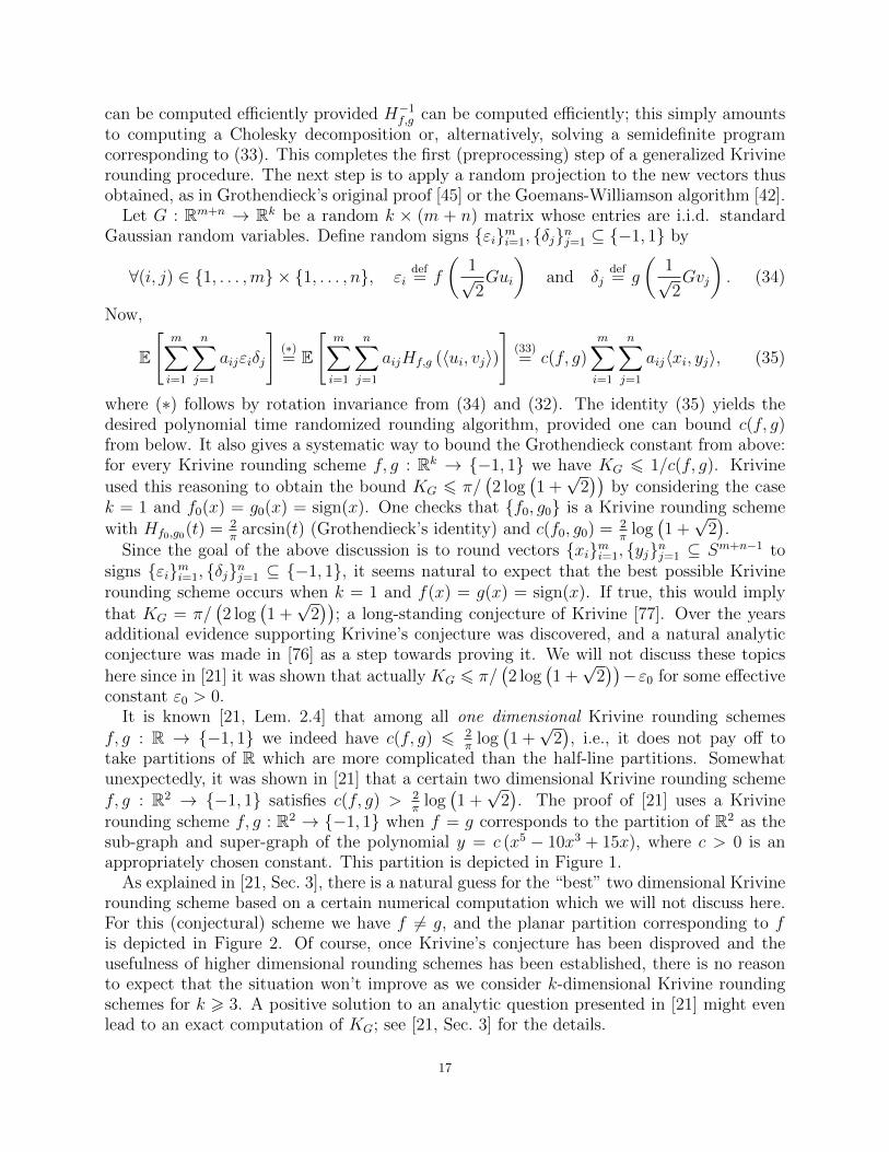
rounding scheme f, g : R2 → −1, 1 when f = g corresponds to the partition of R2 as thesub-graph and super-graph of the polynomial y = c (x5 − 10x3 + 15x), where c > 0 is anappropriately chosen constant. This partition is depicted in Figure 1.
As explained in [21, Sec. 3], there is a natural guess for the “best” two dimensional Krivinerounding scheme based on a certain numerical computation which we will not discuss here.For this (conjectural) scheme we have f 6= g, and the planar partition corresponding to fis depicted in Figure 2. Of course, once Krivine’s conjecture has been disproved and theusefulness of higher dimensional rounding schemes has been established, there is no reasonto expect that the situation won’t improve as we consider k-dimensional Krivine roundingschemes for k > 3. A positive solution to an analytic question presented in [21] might evenlead to an exact computation of KG; see [21, Sec. 3] for the details.
17
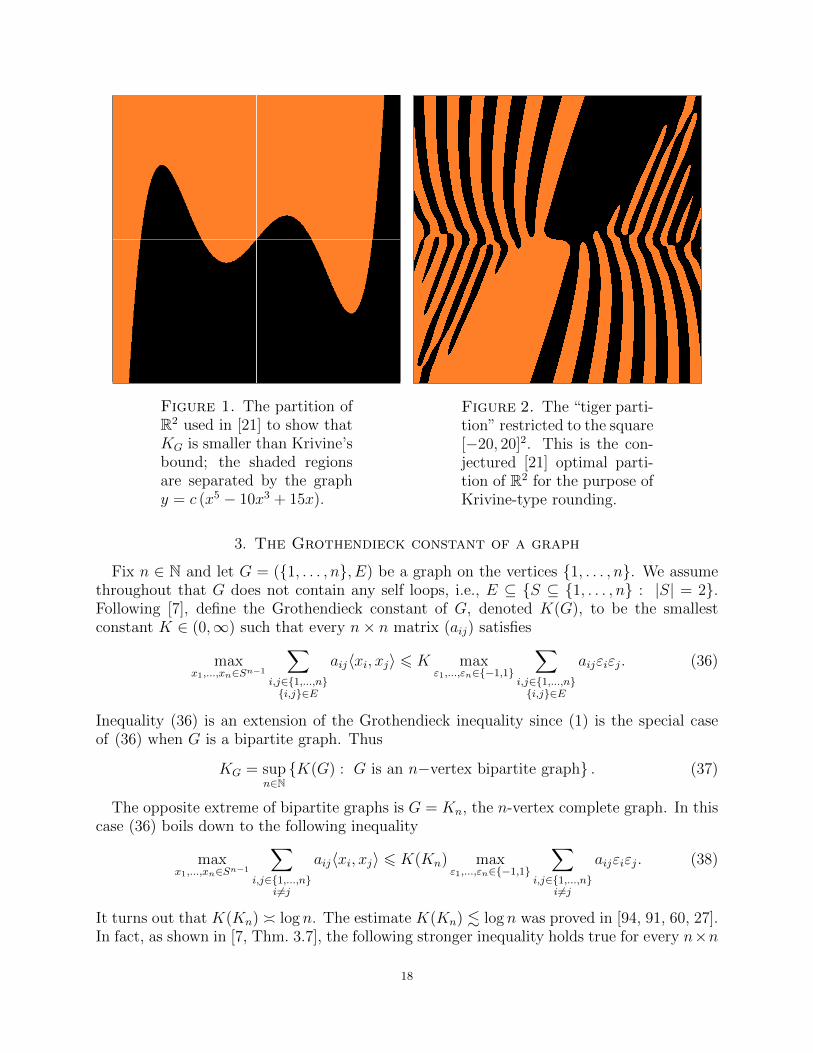
Figure 1. The partition ofR2 used in [21] to show thatKG is smaller than Krivine’sbound; the shaded regionsare separated by the graphy = c (x5 − 10x3 + 15x).
Figure 2. The “tiger parti-tion” restricted to the square[−20, 20]2. This is the con-jectured [21] optimal parti-tion of R2 for the purpose ofKrivine-type rounding.
3. The Grothendieck constant of a graph
Fix n ∈ N and let G = (1, . . . , n, E) be a graph on the vertices 1, . . . , n. We assumethroughout that G does not contain any self loops, i.e., E ⊆ S ⊆ 1, . . . , n : |S| = 2.Following [7], define the Grothendieck constant of G, denoted K(G), to be the smallestconstant K ∈ (0,∞) such that every n× n matrix (aij) satisfies
maxx1,...,xn∈Sn−1
∑i,j∈1,...,ni,j∈E
aij〈xi, xj〉 6 K maxε1,...,εn∈−1,1
∑i,j∈1,...,ni,j∈E
aijεiεj. (36)
Inequality (36) is an extension of the Grothendieck inequality since (1) is the special caseof (36) when G is a bipartite graph. Thus
KG = supn∈NK(G) : G is an n−vertex bipartite graph . (37)
The opposite extreme of bipartite graphs is G = Kn, the n-vertex complete graph. In thiscase (36) boils down to the following inequality
maxx1,...,xn∈Sn−1
∑i,j∈1,...,n
i 6=j
aij〈xi, xj〉 6 K(Kn) maxε1,...,εn∈−1,1
∑i,j∈1,...,n
i 6=j
aijεiεj. (38)
It turns out that K(Kn) log n. The estimate K(Kn) . log n was proved in [94, 91, 60, 27].In fact, as shown in [7, Thm. 3.7], the following stronger inequality holds true for every n×n
18
matrix (aij); it implies that K(Kn) . log n by the Cauchy-Schwartz inequality.
maxx1,...,xn∈Sn−1
∑i,j∈1,...,n
i 6=j
aij〈xi, xj〉
. log
∑i∈1,...,n
∑j∈1,...,nri |aij|√∑
i∈1,...,n∑
j∈1,...,nri a2ij
maxε1,...,εn∈−1,1
∑i,j∈1,...,n
i 6=j
aijεiεj.
The matching lower bound K(Kn) & log n is due to [7], improving over a result of [60].How can we interpolate between the two extremes (37) and (38)? The Grothendieck
constant K(G) depends on the combinatorial structure of the graph G, but at present ourunderstanding of this dependence is incomplete. The following general bounds are known.
logω . K(G) . log ϑ, (39)
andK(G) 6
π
2 log
(1+√
(ϑ−1)2+1
ϑ−1
) , (40)
where (39) is due to [7] and (40) is due to [23]. Here ω is the clique number of G, i.e.,the largest k ∈ 2, . . . , n such that there exists S ⊆ 1, . . . , n of cardinality k satisfyingi, j ∈ E for all distinct i, j ∈ S, and
ϑ = min
max
i∈1,...,n
1
〈xi, y〉2: x1, . . . , xn, y ∈ Sn ∧ ∀i, j ∈ E, 〈xi, xj〉 = 0
. (41)
The parameter ϑ is known as the Lovasz theta function of the complement of G; animportant graph parameter that was introduced in [87]. We refer to [59] and [7, Thm. 3.5]for alternative characterizations of ϑ. It suffices to say here that it was shown in [87] thatϑ 6 χ, where χ is the chromatic number of G, i.e., the smallest integer k such that thereexists a partition A1, . . . , Ak of 1, . . . , n such that i, j /∈ E for all (i, j) ∈
⋃k`=1A`×A`.
Note that the upper bound in (39) is superior to (40) when ϑ is large, but when ϑ = 2 thebound (40) implies Krivine’s classical bound [77] KG 6 π/
(2 log
(1 +√
2))
.The upper and lower bounds in (39) are known to match up to absolute constants for a
variety of graph classes. Several such sharp Grothendieck-type inequalities are presented inSections 5.2 and 5.3 of [7] . For example, as explained in [7], it follows from (39), combinedwith combinatorial results of [87, 9], that for every n× n× n 3-tensor (aijk) we have
maxxijni,j=1⊆Sn
2−1
∑i,j,k∈1,...,n
i 6=j 6=k
aijk 〈xij, xjk〉 . maxεijni,j=1⊆−1,1
∑i,j,k∈1,...,n
i 6=j 6=k
aijkεijεjk.
While (39) is often a satisfactory asymptotic evaluation of K(G), this isn’t always thecase. In particular, it is unknown whether K(G) can be bounded from below by a functionof ϑ that tends to ∞ as ϑ → ∞. An instance in which (39) is not sharp is the case ofErdos-Renyi [36] random graphs G(n, 1/2). For such graphs we have ω log n almostsurely as n → ∞; see [90] and [10, Sec. 4.5]. At the same time, for G(n, 1/2) we have [58]ϑ √n almost surely as n→∞. Thus (39) becomes in this case the rather weak estimate
log log n . K(G(n, 1/2)) . log n. It turns out [3] that K(G(n, 1/2)) log n almost surely as
19
n→∞; we refer to [3] for additional computations of this type of the Grothendieck constantof random and psuedo-random graphs. An explicit evaluation of the Grothendieck constantof certain graph families can be found in [79]; for example, if G is a graph of girth g that is
not a forest and does not admit K5 as a minor then K(G) = g cos(π/g)g−2
.
3.1. Algorithmic consequences. Other than being a natural variant of the Grothendieckinequality, and hence of intrinsic mathematical interest, (36) has ramifications to discreteoptimization problems, which we now describe.
3.1.1. Spin glasses. Perhaps the most natural interpretation of (36) is in the context of solidstate physics, specifically the problem of efficient computation of ground states of Ising spinglasses. The graph G represents the interaction pattern of n particles; thus i, j /∈ E if andonly if the particles i and j cannot interact with each other. Let aij be the magnitude ofthe interaction of i and j (the sign of aij corresponds to attraction/repulsion). In the Isingmodel each particle i ∈ 1, . . . , n has a spin εi ∈ −1, 1 and the total energy of the systemis given by the quantity −
∑i,j∈E aijεiεj. A spin configuration (ε1, . . . , εn) ∈ −1, 1n is
called a ground state if it minimizes the total energy. Thus the problem of finding a groundstate is precisely that of computing the maximum appearing in the right hand side of (36).For more information on this topic see [88, pp. 352–355].
Physical systems seek to settle at a ground state, and therefore it is natural to ask whetherit is computationally efficient (i.e., polynomial time computable) to find such a ground state,at least approximately. Such questions have been studied in the physics literature for severaldecades; see [18, 16, 13, 22]. In particular, it was shown in [16] that if G is a planar graphthen one can find a ground state in polynomial time, but in [13] it was shown that when Gis the three dimensional grid then this computational task is NP-hard.
Since the quantity in the left hand side of (36) is a semidefinite program and thereforecan be computed in polynomial time with arbitrarily good precision, a good bound onK(G) yields a polynomial time algorithm that computes the energy of a ground state withcorrespondingly good approximation guarantee. Moreover, as explained in [7], the proof ofthe upper bound in (39) yields a polynomial time algorithm that finds a spin configuration(σ1, . . . , σn) ∈ −1, 1n for which∑
i,j∈1,...,ni,j∈E
aijσiσj &1
log ϑ· maxεini=1⊆−1,1
∑i,j∈1,...,ni,j∈E
aijεiεj. (42)
An analogous polynomial time algorithm corresponds to the bound (40). These algorithmsyield the best known efficient methods for computing a ground state of Ising spin glasses ona variety of interaction graphs.
3.1.2. Correlation clustering. A different interpretation of (36) yields the best known poly-nomial time approximation algorithm for the correlation clustering problem [14, 25]; this con-nection is due to [27]. Interpret the graph G = (1, . . . , n, E) as the “similarity/dissmilaritygraph” for the items 1, . . . , n, in the following sense. For i, j ∈ E we are given a signaij ∈ −1, 1 which has the following meaning: if aij = 1 then i and j are deemed to besimilar, and if aij = −1 then i and j are deemed to be different. If i, j /∈ E then we donot express any judgement on the similarity or dissimilarity of i and j.
20
Assume that A1, . . . , Ak is a partition (or “clustering”) of 1, . . . , n. An agreement be-tween this clustering and our similarity/dissmilarity judgements is a pair i, j ∈ 1, . . . , nsuch that aij = 1 and i, j ∈ Ar for some r ∈ 1, . . . , k or aij = −1 and i ∈ Ar, j ∈ Asfor distinct r, s ∈ 1, . . . , k. A disagreement between this clustering and our similar-ity/dissmilarity judgements is a pair i, j ∈ 1, . . . , n such that aij = 1 and i ∈ Ar, j ∈ Asfor distinct r, s ∈ 1, . . . , k or aij = −1 and i, j ∈ Ar for some r ∈ 1, . . . , k. Our goal is tocluster the items while encouraging agreements and penalizing disagreements. Thus, we wishto find a clustering of 1, . . . , n into an unspecified number of clusters which maximizes thetotal number of agreements minus the total number of disagreements.
It was proved in [27] that the case of clustering into two parts is the “bottleneck” for thisproblem: if there were a polynomial time algorithm that finds a clustering into two partsfor which the total number of agreements minus the total number of disagreements is atleast a fraction α ∈ (0, 1) of the maximum possible (over all bi-partitions) total number ofagreements minus the total number of disagreements, then one could find in polynomial timea clustering which is at least a fraction α/(2 +α) of the analogous maximum that is definedwithout specifying the number of clusters.
One checks that the problem of finding a partition into two clusters that maximizes thetotal number of agreements minus the total number of disagreements is the same as theproblem of computing the maximum in the right hand side of (36). Thus the upper boundin (39) yields a polynomial time algorithm for correlation clustering with approximationguarantee O(log ϑ), which is the best known approximation algorithm for this problem.Note that when G is the complete graph then the approximation ratio is O(log n). Aswill be explained in Section 7, it is known [69] that for every γ ∈ (0, 1/6), if there were apolynomial time algorithm for correlation clustering that yields an approximation guaranteeof (log n)γ then there would be an algorithm for 3-colorability that runs in time 2(logn)O(1)
, aconclusion which is widely believed to be impossible.
4. Kernel clustering and the propeller conjecture
Here we describe a large class of Grothendieck-type inequalities that is motivated byalgorithmic applications to a combinatorial optimization problem called Kernel Clustering.This problem originates in machine learning [110], and its only known rigorous approximationalgorithms follow from Grothendieck inequalities (these algorithms are sharp assuming theUGC). We will first describe the inequalities and then the algorithmic application.
Consider the special case of the Grothendieck inequality (1) where A = (aij) is an n × npositive semidefinite matrix. In this case we may assume without loss of generality thatin (1) xi = yi and εi = δi for every i ∈ 1, . . . , n since this holds for the maxima on eitherside of (1) (see also the explanation in [8, Sec. 5.2]). It follows from [45, 107] (see also [95])that for every n× n symmetric positive semidefinite matrix A = (aij) we have
maxx1,...,xn∈Sn−1
n∑i=1
n∑j=1
aij〈xi, xj〉 6π
2· maxε1,...,εn∈−1,1
n∑i=1
n∑j=1
aijεiεj, (43)
and that π2
is the best possible constant in (43).
A natural variant of (43) is to replace the numbers −1, 1 by general vectors v1, . . . , vk ∈ Rk,namely one might ask for the smallest constant K ∈ (0,∞) such that for every symmetric
21

positive semidefinite n× n matrix (aij) we have:
maxx1,...,xn∈Sn−1
n∑i=1
n∑j=1
aij〈xi, xj〉 6 K maxu1,...,un∈v1,...,vk
n∑i=1
n∑j=1
aij〈ui, uj〉. (44)
The best constant K in (44) can be characterized as follows. Let B = (bij = 〈vi, vj〉) be theGram matrix of v1, . . . , vk. Let C(B) be the maximum over all partitions A1, . . . , Ak of
Rk−1 into measurable sets of the quantity∑k
i=1
∑kj=1 bij〈zi, zj〉, where for i ∈ 1, . . . , k the
vector zi ∈ Rk−1 is the Gaussian moment of Ai, i.e.,
zi =1
(2π)(k−1)/2
∫Ai
xe−‖x‖22/2dx.
It was proved in [67] that (44) holds with K = 1/C(B) and that this constant is sharp.Inequality (44) with K = 1/C(B) is proved via the following rounding procedure. Fix unit
vectors x1, . . . , xn ∈ Sn−1. Let G = (gij) be a (k − 1) × n random matrix whose entriesare i.i.d. standard Gaussian random variables. Let A1, . . . , Ak ⊆ Rk−1 be a measurablepartition of Rk−1 at which C(B) is attained (for a proof that the maximum defining C(B) isindeed attained, see [67]). Define a random choice of ui ∈ v1, . . . , vk by setting ui = v` forthe unique ` ∈ 1, . . . , k such that Gxi ∈ A`. The fact that (44) holds with K = 1/C(B) isa consequence of the following fact, whose proof we skip (the full details are in [67]).
E
[n∑i=1
n∑j=1
aij〈ui, uj〉
]> C(B)
n∑i=1
n∑j=1
aij〈xi, xj〉. (45)
Determining the partition of Rk−1 that achieves the value C(B) is a nontrivial problem ingeneral, even in the special case when B = Ik is the k× k identity matrix. Note that in thiscase one desires a partition A1, . . . , Ak of Rk−1 into measurable sets so as to maximize thefollowing quantity.
k∑i=1
∥∥∥∥ 1
(2π)(k−1)/2
∫Ai
xe−‖x‖22/2dx
∥∥∥∥2
2
.
As shown in [66, 67], the optimal partition is given by simplicial cones centered at the origin.When B = I2 we have C(I2) = 1
π, and the optimal partition of R into two cones is the
positive and the negative axes. When B = I3 it was shown in [66] that C(I3) = 98π
, and theoptimal partition of R2 into three cones is the propeller partition, i.e., into three cones withangular measure 120 each.
Though it might be surprising at first sight, the authors posed in [66] the propeller con-jecture: for any k > 4, the optimal partition of Rk−1 into k parts is P ×Rk−3 where P is thepropeller partition of R2. In other words, even if one is allowed to use k parts, the propellerconjecture asserts that the best partition consists of only three nonempty parts. Recently,this conjecture was solved positively [53] for k = 4, i.e., for partitions of R3 into four mea-surable parts. The proof of [53] reduces the problem to a concrete finite set of numericalinequalities which are then verified with full rigor in a computer-assisted fashion. Note thatthis is the first nontrivial (surprising?) case of the propeller conjecture, i.e., this is the firstcase in which we indeed drop one of the four allowed parts in the optimal partition.
22
We now describe an application of (44) to the Kernel Clustering problem; a general frame-work for clustering massive statistical data so as to uncover a certain hypothesized struc-ture [110]. The problem is defined as follows. Let A = (aij) be an n× n symmetric positivesemidefinite matrix which is usually normalized to be centered, i.e.,
∑ni=1
∑nj=1 aij = 0. The
matrix A is often thought of as the correlation matrix of random variables (X1, . . . , Xn) thatmeasure attributes of certain empirical data, i.e., aij = E [XiXj]. We are also given anothersymmetric positive semidefinite k × k matrix B = (bij) which functions as a hypothesis, ortest matrix. Think of n as huge and k as a small constant. The goal is to cluster A so asto obtain a smaller matrix which most resembles B. Formally, we wish to find a partitionS1, . . . , Sk of 1, . . . , n so that if we write cij =
∑(p,q)∈Si×Sj apq then the resulting clus-
tered version of A has the maximum correlation∑k
i=1
∑kj=1 cijbij with the hypothesis matrix
B. In words, we form a k× k matrix C = (cij) by summing the entries of A over the blocksinduced by the given partition, and we wish to produce in this way a matrix that is mostcorrelated with B. Equivalently, the goal is to evaluate the number:
Clust(A|B) = maxσ:1,...,n→1,...,k
k∑i=1
k∑j=1
aijbσ(i)σ(j). (46)
The strength of this generic clustering framework is based in part on the flexibility ofadapting the matrix B to the problem at hand. Various particular choices of B lead to wellstudied optimization problems, while other specialized choices of B are based on statisticalhypotheses which have been applied with some empirical success. We refer to [110, 66] foradditional background and a discussion of specific examples.
In [66] it was shown that there exists a randomized polynomial time algorithm that takesas input two positive semidefinite matrices A,B and outputs a number α that satisfiesClust(A|B) 6 E[α] 6
(1 + 3π
2
)Clust(A|B). There is no reason to believe that the approxi-
mation factor of 1 + 3π2
is sharp, but nevertheless prior to this result, which is based on (44),no constant factor polynomial time approximation algorithm for this problem was known.
Sharper results can be obtained if we assume that the input matrices are normalizedappropriately. Specifically, assume that k > 3 and restrict only to inputs A that arecentered, i.e.,
∑ni=1
∑nj=1 aij = 0, and inputs B that are either the identity matrix Ik,
or satisfy∑k
i=1
∑kj=1 bij = 0 (B is centered as well) and bii = 1 for all i ∈ 1, . . . , k
(B is “spherical”). Under these assumptions the output of the algorithm of [66] satisfiesClust(A|B) 6 E[α] 6 8π
9
(1− 1
k
)Clust(A|B). Moreover, it was shown in [66] that assum-
ing the propeller conjecture and the UGC, no polynomial time algorithm can achieve anapproximation guarantee that is strictly smaller than 8π
9
(1− 1
k
)(for input matrices normal-
ized as above). Since the propeller conjecture is known to hold true for k = 3 [66] and k = 4[53], we know that the UGC hardness threshold for the above problem is exactly 16π
27when
k = 3 and 2π3
when k = 4.A finer, and perhaps more natural, analysis of the kernel clustering problem can be ob-
tained if we fix the matrix B and let the input be only the matrix A, with the goal being, asbefore, to approximate the quantity Clust(A|B) in polynomial time. Since B is symmetricand positive semidefinite we can find vectors v1, . . . , vk ∈ Rk such that B is their Grammatrix, i.e., bij = 〈vi, vj〉 for all i, j ∈ 1, . . . , k. Let R(B) be the smallest possible radiusof a Euclidean ball in Rk which contains v1, . . . , vk and let w(B) be the center of this ball.
23
We note that both R(B) and w(B) can be efficiently computed by solving an appropriatesemidefinite program. Let C(B) be the parameter defined above.
It is shown in [67] that for every fixed symmetric positive semidefinite k × k matrix Bthere exists a randomized polynomial time algorithm which given an n×n symmetric positivesemidefinite centered matrix A, outputs a number Alg(A) such that
Clust(A|B) 6 E [Alg(A)] 6R(B)2
C(B)Clust(A|B).
As we will explain in Section 7, assuming the UGC no polynomial time algorithm can achievean approximation guaranty strictly smaller than R(B)2/C(B).
The algorithm of [67] uses semidefinite programming to compute the value
SDP(A|B) = max
n∑i=1
n∑j=1
aij 〈xi, xj〉 : x1, . . . , xn ∈ Rn ∧ ‖xi‖2 6 1 ∀i ∈ 1, . . . , n
= max
n∑i=1
n∑j=1
aij 〈xi, xj〉 : x1, . . . , xn ∈ Sn−1
, (47)
where the last equality in (47) holds since the function (x1, . . . , xn) 7→∑n
i=1
∑nj=1 aij 〈xi, xj〉
is convex (by virtue of the fact that A is positive semidefinite). We claim that
Clust(A|B)
R(B)26 SDP(A|B) 6
Clust(A|B)
C(B), (48)
which implies that if we output the number R(B)2SDP(A|B) we will obtain a polynomial
time algorithm which approximates Clust(A|B) up to a factor of R(B)2
C(B). To verify (48) let
x∗1, . . . , x∗n ∈ Sn−1 and σ∗ : 1, . . . , n → 1, . . . , k be such that
SDP(A|B) =n∑i=1
n∑j=1
aij⟨x∗i , x
∗j
⟩and Clust(A|B) =
n∑i=1
n∑j=1
aijbσ∗(i)σ∗(j).
Write (aij)ni,j=1 = (〈ui, uj〉)ni,j=1 for some u1, . . . , un ∈ Rn. The assumption that A is
centered means that∑n
i=1 ui = 0. The rightmost inequality in (48) is just the Grothendieck
inequality (44). The leftmost inequality in (48) follows from the fact thatvσ∗(i)−w(B)
R(B)has
norm at most 1 for all i ∈ 1, . . . , n. Indeed, these norm bounds imply that
SDP(A|B) >n∑i=1
n∑j=1
aij
⟨vσ∗(i) − w(B)
R(B),vσ∗(j) − w(B)
R(B)
⟩
=1
R(B)2
n∑i=1
n∑j=1
aij⟨vσ∗(i), vσ∗(j)
⟩− 2
R(B)2
n∑i=1
⟨w(B), vσ∗(i)
⟩⟨ui,
n∑j=1
uj
⟩+‖w(B)‖2
2
R(B)2
n∑i=1
n∑j=1
aij
=Clust(A|B)
R(B)2.
24
This completes the proof that the above algorithm approximates efficiently the numberClust(A|B), but does not address the issue of how to efficiently compute an assignmentσ : 1, . . . , n → 1, . . . , k for which the induced clustering of A has the required value.The issue here is to find efficiently a conical simplicial partition A1, . . . , Ak of Rk−1 at whichC(B) is attained. Such a partition exists and may be assumed to be hardwired into thedescription of the algorithm. Alternately, the partition that achieves C(B) up to a desireddegree of accuracy can be found by brute-force for fixed k (or k = k(n) growing sufficientlyslowly as a function of n); see [67]. For large values of k the problem of computing C(B)efficiently remains open.
5. The Lp Grothendieck problem
Fix p ∈ [1,∞] and consider the following algorithmic problem. The input is an n × nmatrix A = (aij) whose diagonal entries vanish, and the goal is to compute (or estimate) inpolynomial time the quantity
Mp(A) = maxt1,...,tn∈R∑nk=1 |tk|p61
n∑i=1
n∑j=1
aijtitj = maxt1,...,tn∈R∑nk=1 |tk|p=1
n∑i=1
n∑j=1
aijtitj. (49)
The second equality in (49) follows from a straightforward convexity argument since thediagonal entries of A vanish. Some of the results described below hold true without the van-ishing diagonal assumption, but we will tacitly make this assumption here since the secondequality in (49) makes the problem become purely combinatorial when p =∞. Specifically,if G = (1, . . . , n, E) is the complete graph then M∞(A) = maxε1,...,εn∈−1,1
∑i,j∈E aijεiεj.
The results described in Section 3 therefore imply that there is a polynomial time algorithmthat approximates M∞(A) up to a O(log n) factor, and that it is computationally hard toachieve an approximation guarantee smaller than (log n)γ for all γ ∈ (0, 1/6).
There are values of p for which the above problem can be solved in polynomial time.When p = 2 the quantity M2(A) is the largest eigenvalue of A, and hence can be computedin polynomial time [43, 82]. When p = 1 it was shown in [2] that it is possible to approximateM1(A) up to a factor of 1 + ε in time nO(1/ε). It is also shown in [2] that the problem of(1 + ε)-approximately computing M1(A) is W [1] complete; we refer to [35] for the definitionof this type of hardness result and just say here that it indicates that a running time ofc(ε)nO(1) is impossible.
The algorithm of [2] proceeds by showing that for every m ∈ N there exist y1, . . . , yn ∈ 1mZ
with∑n
i=1 |yi| 6 1 and∑n
i=1
∑nj=1 aijyiyj >
(1− 1
m
)M1(A). The number of such vectors y
is 1 +∑m
k=1
∑k`=1 2`
(n`
)(k−1`−1
)6 4nm. An exhaustive search over all such vectors will then
approximate M1(A) to within a factor of m/(m− 1) in time O(nm). To prove the existenceof y fix t1, . . . , tn ∈ R with
∑nk=1 |tk| = 1 and
∑ni=1
∑nj=1 aijtitj = M1(A). Let X ∈ Rn be
a random vector given by Pr [X = sign(tj)ej] = |tj| for every j ∈ 1, . . . , n. Here e1, . . . , enis the standard basis of Rn. Let Xs = (Xs1, . . . , Xsn)ms=1 be independent copies of Xand set Y = (Y1, . . . , Yn) = 1
m
∑ms=1Xs. Note that if s, t ∈ 1, . . . ,m are distinct then
for all i, j ∈ 1, . . . , n we have E [XsiXtj] = sign(ti)sign(tj)|ti| · |tj| = titj. Also, for everys ∈ 1, . . . ,m and every distinct i, j ∈ 1, . . . , n we have XsiXsj = 0. Since the diagonal
25
entries of A vanish it follows that
E
[n∑i=1
n∑j=1
aijYiYj
]=
1
m2
∑s,t∈1,...,m
s 6=t
∑i,j∈1,...,n
i 6=j
aijE [XsiXtj] =
(1− 1
m
)M1(A). (50)
Noting that the vector Y has `1 norm at most 1 and all of its entries are integer multiples of1/m, it follows from (50) that with positive probability Y will have the desired properties.
How can we interpolate between the above results for p ∈ 1, 2,∞? It turns out thatthere is a satisfactory answer for p ∈ (2,∞) but the range p ∈ (1, 2) remains a mystery. To
explain this write γp = (E [|G|p])1/p, where G is a standard Gaussian random variable. Onecomputes that
γp =√
2
(Γ(p+1
2
)√π
)1/p
. (51)
Also, Stirling’s formula implies that γ2p = p
e+ O(1) as p → ∞. It follows from [92, 48] that
for every fixed p ∈ [2,∞) there exists a polynomial time algorithm that approximates Mp(A)to within a factor of γ2
p , and that for every ε ∈ (0, 1) the existence of a polynomial time
algorithm that approximates Mp(A) to within a factor γ2p − ε would imply that P = NP .
These results improve over the earlier work [70] which designed a polynomial time algorithmfor Mp(A) whose approximation guarantee is (1 + o(1))γ2
p as p → ∞, and which proved a
γ2p − ε hardness results assuming the UGC rather than P 6= NP .The following Grothendieck-type inequality was proved in [92] and independently in [48].
For every n× n matrix A = (aij) and every p ∈ [2,∞) we have
maxx1,...,xn∈Rn∑nk=1 ‖xk‖
p261
n∑i=1
n∑j=1
aij〈xi, xj〉 6 γ2p max
t1,...,tn∈R∑nk=1 |tk|p61
n∑i=1
n∑j=1
aijtitj. (52)
The constant γ2p in (52) is sharp. The validity of (52) implies that Mp(A) can be computed
in polynomial time to within a factor γ2p . This follows since the left hand side of (52) is the
maximum of∑n
i=1
∑nj=1 aijXij, which is a linear functional in the variables (Xij), given the
constraint that (Xij) is a symmetric positive semidefinite matrix and∑n
i=1 Xp/2ii 6 1. The
latter constraint is convex since p > 2, and therefore this problem falls into the frameworkof convex programming that was described in Section 1.2. Thus the left hand side of (52)can be computed in polynomial time with arbitrarily good precision.
Choosing the specific value p = 3 in order to illustrate the current satisfactory state ofaffairs concretely, the NP -hardness threshold of computing max∑n
i=1 |xi|361
∑ni=1
∑nj=1 aijxixj
equals 2/ 3√π. Such a sharp NP -hardness result (with transcendental hardness ratio) is quite
remarkable, since it shows that the geometric algorithm presented above probably yields thebest possible approximation guarantee even when one allows any polynomial time algorithmwhatsoever. Results of this type have been known to hold under the UGC, but this NP -hardness result of [48] seems to be the first time that such an algorithm for a simple to stateproblem was shown to be optimal assuming P 6= NP .
26
When p ∈ [1, 2] one can easily show [92] that
maxx1,...,xn∈Rn∑nk=1 ‖xk‖
p261
n∑i=1
n∑j=1
aij〈xi, xj〉 = maxt1,...,tn∈R∑nk=1 |tk|p61
n∑i=1
n∑j=1
aijtitj. (53)
While the identity (53) seems to indicate the problem of computing Mp(A) in polynomial
time might be easy for p ∈ (1, 2), the above argument fails since the constraint∑n
i=1Xp/2ii 6 1
is no longer convex. This is reflected by the fact that despite (53) the problem of (1 + ε)-approximately computing M1(A) is W [1] complete [2]. It remains open whether for p ∈ (1, 2)one can approximate Mp(A) in polynomial time up to a factor O(1), and no hardness ofapproximation result is known for this problem as well.
Remark 5.1. If p ∈ [2,∞] then for positive semidefinite matrices (aij) the constant γ2p in
the right hand side of (52) can be improved [92] to γ−2p∗ , where here and in what follows
p∗ = p/(p− 1). For p =∞ this estimate coincides with the classical bound [45, 107] that wehave already encountered in (43), and it is sharp in the entire range p ∈ [2,∞]. Moreover,this bound shows that there exists a polynomial time algorithm that takes as input a positivesemidefinite matrix A and outputs a number that is guaranteed to be within a factor γ−2
p∗
of Mp(A). Conversely, the existence of a polynomial time algorithm for this problem whoseapproximation guarantee is strictly smaller than γ−2
p∗ would contradict the UGC [92].
Remark 5.2. The bilinear variant of (52) is an immediate consequence of the Grothendieckinequality (1). Specifically, assume that p, q ∈ [1,∞] and x1, . . . , xm, y1, . . . , yn ∈ Rm+n
satisfy∑m
i=1 ‖xi‖p2 6 1 and
∑nj=1 ‖yj‖
q2 6 1. Write αi = ‖xi‖2 and βj = ‖yj‖2. For an m× n
matrix (aij) the Grothendieck inequality provides ε1, . . . , εm, δ1, . . . , δn ∈ −1, 1 such that∑mi=1
∑nj=1 aij〈xi, yj〉 6 KG
∑mi=1
∑nj=1 aijαiβjεiδj. This establishes the following inequality.
maxximi=1,yjnj=1⊆Rn+m∑m
i=1 ‖xi‖p261∑n
j=1 ‖yj‖q261
m∑i=1
n∑j=1
aij〈xi, yj〉 6 KG · maxsimi=1,tjnj=1⊆R∑m
i=1 |si|p61∑nj=1 |tj |q61
m∑i=1
n∑j=1
aijsitj. (54)
Observe that the maximum on the right hand side of (54) is ‖A‖p→q∗ ; the operator norm ofA acting as a linear operator from (Rm, ‖ · ‖p) to (Rn, ‖ · ‖q∗). Moreover, if p, q > 2 then theleft hand side of (54) can be computed in polynomial time. Thus, for p > 2 > r > 1, thegeneralized Grothendieck inequality (54) yields a polynomial time algorithm that takes asinput an m × n matrix A = (aij) and outputs a number that is guaranteed to be within afactor KG of ‖A‖p→r. This algorithmic task has been previously studied in [96] (see also [93,Sec. 4.3.2]), where for p > 2 > r > 1 a polynomial time algorithm was designed thatapproximates ‖A‖p→r up to a factor 3π/
(6√
3− 2π)∈ [2.293, 2.294]. The above argument
yields the approximation factor KG < 1.783 as a formal consequence of the Grothendieckinequality. The complexity of the problem of approximating ‖A‖p→r has been studied in [17],where it is shown that if either p > r > 2 or 2 > p > r then it is NP -hard to approximate‖A‖p→r up to any constant factor, and unless 3-colorability can be solved in time 2(logn)O(1)
,
for any ε ∈ (0, 1) no polynomial time algorithm can approximate ‖A‖p→r up to 2(logn)1−ε .
Remark 5.3. Let K ⊆ Rn be a compact and convex set which is invariant under reflectionswith respect to the coordinate hyperplanes. Denote by CK the smallest C ∈ (0,∞) such
27
that for every n× n matrix (aij) we have
maxx1,...,xn∈Rn
(‖x1‖2,...,‖xn‖2)∈K
n∑i=1
n∑j=1
aij〈xi, xj〉 6 C maxt1,...,tn∈R
(t1,...,tn)∈K
n∑i=1
n∑j=1
aijtitj. (55)
Such generalized Grothendieck inequalities are investigated in [92], where bounds on CK areobtained under certain geometric assumptions on K. These assumptions are easy to verifywhen K = x ∈ Rn : ‖x‖p 6 1, yielding (52). More subtle inequalities of this type forother convex bodies K are discussed in [92], but we will not describe them here. The naturalbilinear version of (55) is: if K ⊆ Rm and L ⊆ Rn are compact and convex sets that areinvariant under reflections with respect to the coordinate hyperplanes then let CK,L denotethe smallest constant C ∈ (0,∞) such that for every m× n matrix (aij) we have
maxximi=1,yjnj=1⊆Rn+m
(‖x1‖2,...,‖xm‖2)∈K(‖y1‖2,...,‖yn‖2)∈L
m∑i=1
n∑j=1
aij〈xi, yj〉 6 C maxsimi=1,tjnj=1⊆R
(s1,...,sm)∈K(t1,...,tn)∈L
m∑i=1
n∑j=1
aijsitj. (56)
The argument in Remark 5.2 shows that CK,L 6 KG. Under certain geometric assumptionson K,L this bound can be improved [92].
6. Higher rank Grothendieck inequalities
We have already seen several variants of the classical Grothendieck inequality (1), in-cluding the Grothendieck inequality for graphs (36), the variant of the positive semidefiniteGrothendieck inequality arising from the Kernel Clustering problem (44), and Grothendieckinequalities for convex bodies other than the cube (52), (54), (55), (56). The literature con-tains additional variants of the Grothendieck inequality, some of which will be described inthis section.
Let G = (1, . . . , n, E) be a graph and fix q, r ∈ N. Following [23], let K(q → r,G) bethe smallest constant K ∈ (0,∞) such that for every n× n matrix A = (aij) we have
maxx1,...,xn∈Sq−1
∑i,j∈1,...,ni,j∈E
aij〈xi, xj〉 6 K maxy1,...,yn∈Sr−1
∑i,j∈1,...,ni,j∈E
aij〈yi, yj〉. (57)
Set also K(r,G) = supq∈NK(q → r,G). We similarly define K+(q → r,G) to be thesmallest constant K ∈ (0,∞) satisfying (57) for all positive semidefinite matrices A, andcorrespondingly K+(r,G) = supq∈NK
+(q → r,G).To link these definitions to what we have already seen in this article, observe that KG is
the supremum of K(1, G) over all finite bipartite graphs G, and due to the results describedin Section 4 we have
supn∈N
K+ (r,Kn ) = supn∈N
supx1,...,xn∈Sr−1
1
C(〈xi, xj〉)ni,j=1
) , (58)
where Kn is the complete graph on n-vertices with self loops. Recall that the definition ofC(B) for a positive semidefinite matrix B is given in the paragraph following (44).
An important special case of (57) is r = 2, since the supremum of K(2, G) over all finitebipartite graphs G is at most the complex Grothendieck constant KC
G (defined analogouslyto KG, but over the complex scalar field), a fundamental quantity whose value has been
28
investigated in [45, 83, 99, 50, 74]. The best known bounds on KCG are 1.338 < KC
G < 1.4049;see [101, Sec. 4] for more information on this topic. We also refer to [32, 113] for informationof the constants K(2q → 2, G) where G is a bipartite graph. The supremum of K(q → r,G)over all biparpite graphs G was investigated in [78] for r = 1 and in [74] for r = 2; seealso [75] for a unified treatment of these cases. The higher rank constants K(q → r,G)when G is bipartite were introduced in [22]. Definition (57) in full generality is due to [23]where several estimates on K(q → r,G) are given. One of the motivations of [23] is thecase r = 3 (and G a subgraph of the grid Z3), based on the connection to the polynomialtime approximation of ground states of spin glasses as described in Section 3.1.1; the caser = 1 was discussed in Section 3.1.1 in connection with the Ising model, but the case r = 3corresponds to the more physically realistic Heisenberg model of vector-valued spins. Theparameter supn∈NK
+ (r,Kn ) (recall (58)) was studied in [22] in the context of quantuminformation theory, and in [24] it was shown that
K+ (1, Kn ) 6π
n
(Γ((n+ 1)/2)
Γ(n/2)
)2
=π
2− π
4n+O
(1
n2
), (59)
and
supn∈N
K+ (r,Kn ) =r
2
(Γ(r/2)
Γ((r + 1)/2)
)2
= 1 +1
2r+O
(1
r2
).
We refer to [24] for a corresponding UGC hardness result. Note that (59) improves over (43)for fixed n ∈ N.
7. Hardness of approximation
We have seen examples of how Grothendieck-type inequalities yield upper bounds onthe best possible polynomial time approximation ratio of certain optimization problems.From the algorithmic and computational complexity viewpoint it is interesting to provecomputational lower bounds as well, i.e., results that rule out the existence of efficientalgorithms achieving a certain approximation guarantee. Such results are known as hardnessor inapproximability results, and as explained in Section 1.1, at present the state of the artallows one to prove such results while relying on complexity theoretic assumptions such asP 6= NP or the Unique Games Conjecture. A nice feature of the known hardness resultsfor problems in which a Grothendieck-type inequality has been applied is that often thehardness results (lower bounds) exactly match the approximation ratios (upper bounds). Inthis section we briefly review the known hardness results for optimization problems associatedwith Grothendieck-type inequalities.
Let Kn,n-QP denote the optimization problem associated with the classical Grothendieckinequality (the acronym QP stands for “quadratic programming”). Thus, in the problemKn,n-QP we are given an n× n real matrix (aij) and the goal is to determine the quantity
max
m∑i=1
n∑j=1
aijεiδj : εimi=1, δjnj=1 ⊆ −1, 1
.
As explained in [8], the MAX DICUT problem can be framed as a special case of theproblem Kn,n-QP. Hence, as a consequence of [51], we know that for every ε ∈ (0, 1), assum-ing P 6= NP there is no polynomial time algorithm that approximates the Kn,n-QP problemwithin ratio 13
12−ε. In [68] it is shown that the lower bound (3) on the Grothendieck constant
29

can be translated into a hardness result, albeit relying on the Unique Games Conjecture.Namely, letting η0 be as in (3), for every ε ∈ (0, 1) assuming the UGC there is no polynomial
time algorithm that approximates the Kn,n-QP problem within a ratio π2eη
20 − ε.
We note that all the hardness results cited here rely on the well-known paradigm ofdictatorship testing. A lower bound on the integrality gap of a semidefinite program, suchas the estimate KG > π
2eη
20 , can be translated into a probabilistic test to check whether a
function f : −1, 1n 7→ −1, 1 is a dictatorship, i.e., of the form f(x) = xi for some fixedi ∈ 1, . . . , n. If f is indeed a dictatorship, then the test passes with probability c and iff is “far from a dictator” (in a formal sense that we do not describe here), the test passeswith probability at most s. The ratio c/s corresponds exactly to the UGC-based hardnesslower bound. It is well-known how to prove a UGC-based hardness result once we have theappropriate dictatorship test; see the survey [63].
The above quoted result of [68] relied on explicitly knowing the lower bound construc-
tion [105] leading to the estimate KG > π2eη
20 . On the other hand, in [104], building on
the earlier work [103], it is shown that any lower bound on the Grothedieck constant canbe translated into a UGC-based hardness result, even without explicitly knowing the con-struction! Thus, modulo the UGC, the best polynomial time algorithm to approximate theKn,n-QP problem is via the Grothendieck inequality, even though we do not know the precisevalue of KG. Formally, for every ε ∈ (0, 1), assuming the UGC there is no polynomial timealgorithm that approximates the Kn,n-QP problem within a factor KG − ε.
Let Kn,n-QPPSD be the special case of the Kn,n-QP problem where the input matrix (aij) isassumed to be positive semidefinite. By considering matrices that are Laplacians of graphsone sees that the MAX CUT problem is a special case of the problem Kn,n-QPPSD (see [66]).Hence, due to [51], we know that for every ε ∈ (0, 1), assuming P 6= NP there is nopolynomial time algorithm that approximates the Kn,n-QPPSD problem within ratio 17
16− ε.
Moreover, it is proved in [66] that for every ε ∈ (0, 1), assuming the UGC there is nopolynomial time algorithm that approximates the Kn,n-QPPSD problem within ratio π
2− ε,
an optimal hardness result due to the positive semidefinite Grothendieck inequality (43).This follows from the more general results for the Kernel Clustering problem described later.
Let (aij) be an n× n real matrix with zeroes on the diagonal. The Kn-QP problem seeksto determine the quantity
max
m∑i=1
n∑j=1
aijεiεj : εimi=1 ⊆ −1, 1
.
In [69] it is proved that for every γ ∈ (0, 1/6), assuming that NP does not have a 2(logn)O(1)
time deterministic algorithm, there is no polynomial time algorithm that approximates theKn-QP problem within ratio (log n)γ. This improves over [12] where a hardness factor of(log n)c was proved, under the same complexity assumption, for an unspecified universalconstant c > 0. Recall that, as explained in Section 3, there is an algorithm for Kn-QPthat achieves a ratio of O(log n), so there remains an asymptotic gap in our understandingof the complexity of the Kn-QP problem. For the maximum acyclic subgraph problem,as discussed in Section 2.1.3, the gap between the upper and lower bounds is even larger.We have already seen that an approximation factor of O(log n) is achievable, but from thehardness perspective we know due to [97] that there exists ε0 > 0 such that assumingP 6= NP there is no polynomial time algorithm for the maximum acyclic subgraph problem
30
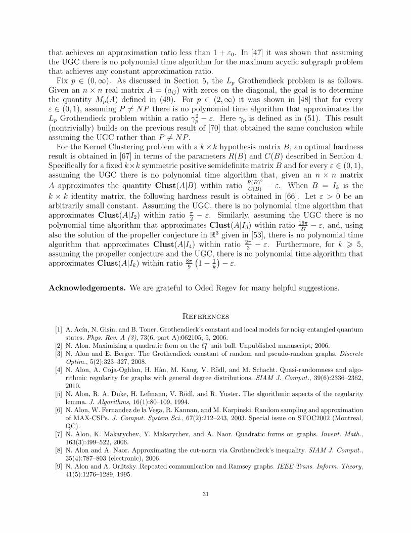
that achieves an approximation ratio less than 1 + ε0. In [47] it was shown that assumingthe UGC there is no polynomial time algorithm for the maximum acyclic subgraph problemthat achieves any constant approximation ratio.
Fix p ∈ (0,∞). As discussed in Section 5, the Lp Grothendieck problem is as follows.Given an n × n real matrix A = (aij) with zeros on the diagonal, the goal is to determinethe quantity Mp(A) defined in (49). For p ∈ (2,∞) it was shown in [48] that for everyε ∈ (0, 1), assuming P 6= NP there is no polynomial time algorithm that approximates theLp Grothendieck problem within a ratio γ2
p − ε. Here γp is defined as in (51). This result(nontrivially) builds on the previous result of [70] that obtained the same conclusion whileassuming the UGC rather than P 6= NP .
For the Kernel Clustering problem with a k×k hypothesis matrix B, an optimal hardnessresult is obtained in [67] in terms of the parameters R(B) and C(B) described in Section 4.Specifically for a fixed k×k symmetric positive semidefinite matrix B and for every ε ∈ (0, 1),assuming the UGC there is no polynomial time algorithm that, given an n × n matrix
A approximates the quantity Clust(A|B) within ratio R(B)2
C(B)− ε. When B = Ik is the
k × k identity matrix, the following hardness result is obtained in [66]. Let ε > 0 be anarbitrarily small constant. Assuming the UGC, there is no polynomial time algorithm thatapproximates Clust(A|I2) within ratio π
2− ε. Similarly, assuming the UGC there is no
polynomial time algorithm that approximates Clust(A|I3) within ratio 16π27− ε, and, using
also the solution of the propeller conjecture in R3 given in [53], there is no polynomial timealgorithm that approximates Clust(A|I4) within ratio 2π
3− ε. Furthermore, for k > 5,
assuming the propeller conjecture and the UGC, there is no polynomial time algorithm thatapproximates Clust(A|Ik) within ratio 8π
9
(1− 1
k
)− ε.
Acknowledgements. We are grateful to Oded Regev for many helpful suggestions.
References
[1] A. Acın, N. Gisin, and B. Toner. Grothendieck’s constant and local models for noisy entangled quantumstates. Phys. Rev. A (3), 73(6, part A):062105, 5, 2006.
[2] N. Alon. Maximizing a quadratic form on the `n1 unit ball. Unpublished manuscript, 2006.[3] N. Alon and E. Berger. The Grothendieck constant of random and pseudo-random graphs. Discrete
Optim., 5(2):323–327, 2008.[4] N. Alon, A. Coja-Oghlan, H. Han, M. Kang, V. Rodl, and M. Schacht. Quasi-randomness and algo-
rithmic regularity for graphs with general degree distributions. SIAM J. Comput., 39(6):2336–2362,2010.
[5] N. Alon, R. A. Duke, H. Lefmann, V. Rodl, and R. Yuster. The algorithmic aspects of the regularitylemma. J. Algorithms, 16(1):80–109, 1994.
[6] N. Alon, W. Fernandez de la Vega, R. Kannan, and M. Karpinski. Random sampling and approximationof MAX-CSPs. J. Comput. System Sci., 67(2):212–243, 2003. Special issue on STOC2002 (Montreal,QC).
[7] N. Alon, K. Makarychev, Y. Makarychev, and A. Naor. Quadratic forms on graphs. Invent. Math.,163(3):499–522, 2006.
[8] N. Alon and A. Naor. Approximating the cut-norm via Grothendieck’s inequality. SIAM J. Comput.,35(4):787–803 (electronic), 2006.
[9] N. Alon and A. Orlitsky. Repeated communication and Ramsey graphs. IEEE Trans. Inform. Theory,41(5):1276–1289, 1995.
31
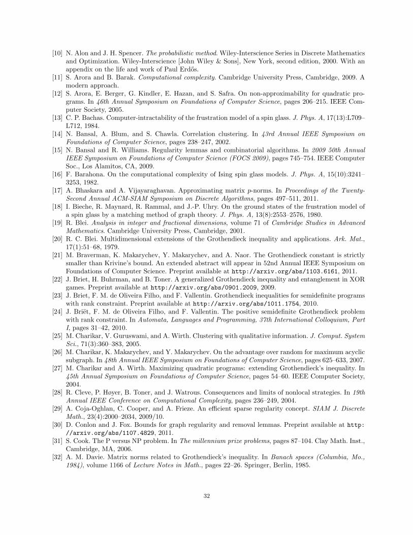
[10] N. Alon and J. H. Spencer. The probabilistic method. Wiley-Interscience Series in Discrete Mathematicsand Optimization. Wiley-Interscience [John Wiley & Sons], New York, second edition, 2000. With anappendix on the life and work of Paul Erdos.
[11] S. Arora and B. Barak. Computational complexity. Cambridge University Press, Cambridge, 2009. Amodern approach.
[12] S. Arora, E. Berger, G. Kindler, E. Hazan, and S. Safra. On non-approximability for quadratic pro-grams. In 46th Annual Symposium on Foundations of Computer Science, pages 206–215. IEEE Com-puter Society, 2005.
[13] C. P. Bachas. Computer-intractability of the frustration model of a spin glass. J. Phys. A, 17(13):L709–L712, 1984.
[14] N. Bansal, A. Blum, and S. Chawla. Correlation clustering. In 43rd Annual IEEE Symposium onFoundations of Computer Science, pages 238–247, 2002.
[15] N. Bansal and R. Williams. Regularity lemmas and combinatorial algorithms. In 2009 50th AnnualIEEE Symposium on Foundations of Computer Science (FOCS 2009), pages 745–754. IEEE ComputerSoc., Los Alamitos, CA, 2009.
[16] F. Barahona. On the computational complexity of Ising spin glass models. J. Phys. A, 15(10):3241–3253, 1982.
[17] A. Bhaskara and A. Vijayaraghavan. Approximating matrix p-norms. In Proceedings of the Twenty-Second Annual ACM-SIAM Symposium on Discrete Algorithms, pages 497–511, 2011.
[18] I. Bieche, R. Maynard, R. Rammal, and J.-P. Uhry. On the ground states of the frustration model ofa spin glass by a matching method of graph theory. J. Phys. A, 13(8):2553–2576, 1980.
[19] R. Blei. Analysis in integer and fractional dimensions, volume 71 of Cambridge Studies in AdvancedMathematics. Cambridge University Press, Cambridge, 2001.
[20] R. C. Blei. Multidimensional extensions of the Grothendieck inequality and applications. Ark. Mat.,17(1):51–68, 1979.
[21] M. Braverman, K. Makarychev, Y. Makarychev, and A. Naor. The Grothendieck constant is strictlysmaller than Krivine’s bound. An extended abstract will appear in 52nd Annual IEEE Symposium onFoundations of Computer Science. Preprint available at http://arxiv.org/abs/1103.6161, 2011.
[22] J. Briet, H. Buhrman, and B. Toner. A generalized Grothendieck inequality and entanglement in XORgames. Preprint available at http://arxiv.org/abs/0901.2009, 2009.
[23] J. Briet, F. M. de Oliveira Filho, and F. Vallentin. Grothendieck inequalities for semidefinite programswith rank constraint. Preprint available at http://arxiv.org/abs/1011.1754, 2010.
[24] J. Briet, F. M. de Oliveira Filho, and F. Vallentin. The positive semidefinite Grothendieck problemwith rank constraint. In Automata, Languages and Programming, 37th International Colloquium, PartI, pages 31–42, 2010.
[25] M. Charikar, V. Guruswami, and A. Wirth. Clustering with qualitative information. J. Comput. SystemSci., 71(3):360–383, 2005.
[26] M. Charikar, K. Makarychev, and Y. Makarychev. On the advantage over random for maximum acyclicsubgraph. In 48th Annual IEEE Symposium on Foundations of Computer Science, pages 625–633, 2007.
[27] M. Charikar and A. Wirth. Maximizing quadratic programs: extending Grothendieck’s inequality. In45th Annual Symposium on Foundations of Computer Science, pages 54–60. IEEE Computer Society,2004.
[28] R. Cleve, P. Høyer, B. Toner, and J. Watrous. Consequences and limits of nonlocal strategies. In 19thAnnual IEEE Conference on Computational Complexity, pages 236–249, 2004.
[29] A. Coja-Oghlan, C. Cooper, and A. Frieze. An efficient sparse regularity concept. SIAM J. DiscreteMath., 23(4):2000–2034, 2009/10.
[30] D. Conlon and J. Fox. Bounds for graph regularity and removal lemmas. Preprint available at http:
//arxiv.org/abs/1107.4829, 2011.[31] S. Cook. The P versus NP problem. In The millennium prize problems, pages 87–104. Clay Math. Inst.,
Cambridge, MA, 2006.[32] A. M. Davie. Matrix norms related to Grothendieck’s inequality. In Banach spaces (Columbia, Mo.,
1984), volume 1166 of Lecture Notes in Math., pages 22–26. Springer, Berlin, 1985.
32
[33] J. Diestel, J. H. Fourie, and J. Swart. The metric theory of tensor products. American MathematicalSociety, Providence, RI, 2008. Grothendieck’s resume revisited.
[34] J. Diestel, H. Jarchow, and A. Tonge. Absolutely summing operators, volume 43 of Cambridge Studiesin Advanced Mathematics. Cambridge University Press, Cambridge, 1995.
[35] R. G. Downey and M. R. Fellows. Parameterized complexity. Monographs in Computer Science.Springer-Verlag, New York, 1999.
[36] P. Erdos and A. Renyi. On the evolution of random graphs. Magyar Tud. Akad. Mat. Kutato Int.Kozl., 5:17–61, 1960.
[37] P. C. Fishburn and J. A. Reeds. Bell inequalities, Grothendieck’s constant, and root two. SIAM J.Discrete Math., 7(1):48–56, 1994.
[38] A. Frieze and R. Kannan. Quick approximation to matrices and applications. Combinatorica, 19(2):175–220, 1999.
[39] M. R. Garey and D. S. Johnson. Computers and intractability. W. H. Freeman and Co., San Francisco,Calif., 1979. A guide to the theory of NP-completeness, A Series of Books in the Mathematical Sciences.
[40] D. J. H. Garling. Inequalities: a journey into linear analysis. Cambridge University Press, Cambridge,2007.
[41] S. Gerke and A. Steger. A characterization for sparse ε-regular pairs. Electron. J. Combin., 14(1):Re-search Paper 4, 12 pp. (electronic), 2007.
[42] M. X. Goemans and D. P. Williamson. Improved approximation algorithms for maximum cut andsatisfiability problems using semidefinite programming. J. Assoc. Comput. Mach., 42(6):1115–1145,1995.
[43] G. H. Golub and C. F. Van Loan. Matrix computations. Johns Hopkins Studies in the MathematicalSciences. Johns Hopkins University Press, Baltimore, MD, third edition, 1996.
[44] W. T. Gowers. Lower bounds of tower type for Szemeredi’s uniformity lemma. Geom. Funct. Anal.,7(2):322–337, 1997.
[45] A. Grothendieck. Resume de la theorie metrique des produits tensoriels topologiques. Bol. Soc. Mat.Sao Paulo, 8:1–79, 1953.
[46] M. Grotschel, L. Lovasz, and A. Schrijver. Geometric algorithms and combinatorial optimization, vol-ume 2 of Algorithms and Combinatorics. Springer-Verlag, Berlin, second edition, 1993.
[47] V. Guruswami, R. Manokaran, and P. Raghavendra. Beating the random ordering is hard: Inapprox-imability of maximum acyclic subgraph. In 49th Annual IEEE Symposium on Foundations of ComputerScience, pages 573–582, 2008.
[48] V. Guruswami, P. Raghavendra, R. Saket, and Y. Wu. Bypassing UGC from some optimal geometricinapproximability results. Electronic Colloquium on Computational Complexity (ECCC), 17:177, 2010.
[49] U. Haagerup. The Grothendieck inequality for bilinear forms on C∗-algebras. Adv. in Math., 56(2):93–116, 1985.
[50] U. Haagerup. A new upper bound for the complex Grothendieck constant. Israel J. Math., 60(2):199–224, 1987.
[51] J. Hastad. Some optimal inapproximability results. J. ACM, 48(4):798–859 (electronic), 2001.[52] J. Hastad and S. Venkatesh. On the advantage over a random assignment. Random Structures Algo-
rithms, 25(2):117–149, 2004.[53] S. Heilman, A. Jagannath, and A. Naor. Solution of the propeller conjecture in R3. Manuscript, 2011.[54] H. Heydari. Quantum correlation and Grothendieck’s constant. J. Phys. A, 39(38):11869–11875, 2006.[55] G. J. O. Jameson. Summing and nuclear norms in Banach space theory, volume 8 of London Mathe-
matical Society Student Texts. Cambridge University Press, Cambridge, 1987.[56] W. B. Johnson and J. Lindenstrauss. Basic concepts in the geometry of Banach spaces. In Handbook
of the geometry of Banach spaces, Vol. I, pages 1–84. North-Holland, Amsterdam, 2001.[57] D. B. Judin and A. S. Nemirovskiı. Informational complexity and effective methods for the solution of
convex extremal problems. Ekonom. i Mat. Metody, 12(2):357–369, 1976.[58] F. Juhasz. The asymptotic behaviour of Lovasz’ θ function for random graphs. Combinatorica,
2(2):153–155, 1982.[59] D. Karger, R. Motwani, and M. Sudan. Approximate graph coloring by semidefinite programming. J.
ACM, 45(2):246–265, 1998.
33
[60] B. S. Kashin and S. I. Sharek. On the Gram matrices of systems of uniformly bounded functions. Tr.Mat. Inst. Steklova, 243(Funkts. Prostran., Priblizh., Differ. Uravn.):237–243, 2003.
[61] J. Kempe, H. Kobayashi, K. Matsumoto, B. Toner, and T. Vidick. Entangled games are hard toapproximate. In 49th Annual IEEE Symposium on Foundations of Computer Science, pages 447–456,2008.
[62] S. Khot. On the power of unique 2-prover 1-round games. In Proceedings of the Thirty-Fourth AnnualACM Symposium on Theory of Computing, pages 767–775 (electronic), New York, 2002. ACM.
[63] S. Khot. On the unique games conjecture (invited survey). In Proceedings of the 25th Annual IEEEConference on Computational Complexity, pages 99–121, 2010.
[64] S. Khot, G. Kindler, E. Mossel, and R. O’Donnell. Optimal inapproximability results for MAX-CUTand other 2-variable CSPs? SIAM J. Comput., 37(1):319–357 (electronic), 2007.
[65] S. Khot and A. Naor. Linear equations modulo 2 and the L1 diameter of convex bodies. SIAM J.Comput., 38(4):1448–1463, 2008.
[66] S. Khot and A. Naor. Approximate kernel clustering. Mathematika, 55(1-2):129–165, 2009.[67] S. Khot and A. Naor. Sharp kernel clustering algorithms and their associated Grothendieck inequalities.
In Proceedings of the Twenty-First Annual ACM-SIAM Symposium on Discrete Algorithms, pages 664–683, 2010. Full version to appear in Random Structures and Algorithms.
[68] S. Khot and R. O’Donnell. SDP gaps and UGC-hardness for max-cut-gain. Theory Comput., 5:83–117,2009.
[69] S. Khot and S. Safra. A two prover one round game with strong soundness. To appear in 52nd AnnualIEEE Symposium on Foundations of Computer Science, 2011.
[70] G. Kindler, A. Naor, and G. Schechtman. The UGC hardness threshold of the Lp Grothendieck prob-lem. Math. Oper. Res., 35(2):267–283, 2010.
[71] Y. Kohayakawa. Szemeredi’s regularity lemma for sparse graphs. In Foundations of computationalmathematics (Rio de Janeiro, 1997), pages 216–230. Springer, Berlin, 1997.
[72] Y. Kohayakawa and V. Rodl. Szemeredi’s regularity lemma and quasi-randomness. In Recent advancesin algorithms and combinatorics, volume 11 of CMS Books Math./Ouvrages Math. SMC, pages 289–351.Springer, New York, 2003.
[73] Y. Kohayakawa, V. Rodl, and L. Thoma. An optimal algorithm for checking regularity. SIAM J.Comput., 32(5):1210–1235 (electronic), 2003.
[74] H. Konig. On the complex Grothendieck constant in the n-dimensional case. In Geometry of Banachspaces (Strobl, 1989), volume 158 of London Math. Soc. Lecture Note Ser., pages 181–198. CambridgeUniv. Press, Cambridge, 1990.
[75] H. Konig. Some remarks on the Grothendieck inequality. In General inequalities, 6 (Oberwolfach, 1990),volume 103 of Internat. Ser. Numer. Math., pages 201–206. Birkhauser, Basel, 1992.
[76] H. Konig. On an extremal problem originating in questions of unconditional convergence. In Recentprogress in multivariate approximation (Witten-Bommerholz, 2000), volume 137 of Internat. Ser. Nu-mer. Math., pages 185–192. Birkhauser, Basel, 2001.
[77] J.-L. Krivine. Sur la constante de Grothendieck. C. R. Acad. Sci. Paris Ser. A-B, 284(8):A445–A446,1977.
[78] J.-L. Krivine. Constantes de Grothendieck et fonctions de type positif sur les spheres. Adv. in Math.,31(1):16–30, 1979.
[79] M. Laurent and A. Varvitsiotis. Computing the Grothendieck constant of some graph classes. Preprintavailable at http://arxiv.org/abs/1106.2735, 2011.
[80] T. Lee, G. Schechtman, and A. Shraibman. Lower bounds on quantum multiparty communicationcomplexity. In Proceedings of the 24th Annual IEEE Conference on Computational Complexity, pages254–262, 2009.
[81] T. Lee and A. Shraibman. Lower bounds in communication complexity. Found. Trends Theor. Comput.Sci., 3(4):front matter, 263–399 (2009), 2007.
[82] A. S. Lewis and M. L. Overton. Eigenvalue optimization. In Acta numerica, 1996, volume 5 of ActaNumer., pages 149–190. Cambridge Univ. Press, Cambridge, 1996.
[83] J. Lindenstrauss and A. Pe lczynski. Absolutely summing operators in Lp-spaces and their applications.Studia Math., 29:275–326, 1968.
34
[84] N. Linial, S. Mendelson, G. Schechtman, and A. Shraibman. Complexity measures of sign matrices.Combinatorica, 27(4):439–463, 2007.
[85] N. Linial and A. Shraibman. Learning complexity vs. communication complexity. Combin. Probab.Comput., 18(1-2):227–245, 2009.
[86] N. Linial and A. Shraibman. Lower bounds in communication complexity based on factorization norms.Random Structures Algorithms, 34(3):368–394, 2009.
[87] L. Lovasz. On the Shannon capacity of a graph. IEEE Trans. Inform. Theory, 25(1):1–7, 1979.[88] L. Lovasz and M. D. Plummer. Matching theory, volume 121 of North-Holland Mathematics Studies.
North-Holland Publishing Co., Amsterdam, 1986. Annals of Discrete Mathematics, 29.[89] L. Lovasz and B. Szegedy. Szemeredi’s lemma for the analyst. Geom. Funct. Anal., 17(1):252–270,
2007.[90] D. W. Matula. On the complete subgraphs of a random graph. In Proc. Second Chapel Hill Conf.
on Combinatorial Mathematics and its Applications (Univ. North Carolina, Chapel Hill, N.C., 1970),pages 356–369. Univ. North Carolina, Chapel Hill, N.C., 1970.
[91] A. Megretski. Relaxations of quadratic programs in operator theory and system analysis. In Systems,approximation, singular integral operators, and related topics (Bordeaux, 2000), volume 129 of Oper.Theory Adv. Appl., pages 365–392. Birkhauser, Basel, 2001.
[92] A. Naor and G. Schechtman. An approximation scheme for quadratic form maximization on convexbodies. Manuscript, 2009.
[93] A. Nemirovski. Advances in convex optimization: conic programming. In International Congress ofMathematicians. Vol. I, pages 413–444. Eur. Math. Soc., Zurich, 2007.
[94] A. Nemirovski, C. Roos, and T. Terlaky. On maximization of quadratic form over intersection ofellipsoids with common center. Math. Program., 86(3, Ser. A):463–473, 1999.
[95] Y. Nesterov. Semidefinite relaxation and nonconvex quadratic optimization. Optim. Methods Softw.,9(1-3):141–160, 1998.
[96] Y. Nesterov, H. Wolkowicz, and Y. Ye. Semidefinite programming relaxations of nonconvex quadraticoptimization. In Handbook of semidefinite programming, volume 27 of Internat. Ser. Oper. Res. Man-agement Sci., pages 361–419. Kluwer Acad. Publ., Boston, MA, 2000.
[97] C. H. Papadimitriou and M. Yannakakis. Optimization, approximation, and complexity classes. J.Comput. System Sci., 43(3):425–440, 1991.
[98] D. Perez-Garcıa, M. M. Wolf, C. Palazuelos, I. Villanueva, and M. Junge. Unbounded violation oftripartite Bell inequalities. Comm. Math. Phys., 279(2):455–486, 2008.
[99] G. Pisier. Grothendieck’s theorem for noncommutative C∗-algebras, with an appendix onGrothendieck’s constants. J. Funct. Anal., 29(3):397–415, 1978.
[100] G. Pisier. Factorization of linear operators and geometry of Banach spaces, volume 60 of CBMS Re-gional Conference Series in Mathematics. Published for the Conference Board of the MathematicalSciences, Washington, DC, 1986.
[101] G. Pisier. Grothendieck’s theorem, past and present. Preprint available at http://arxiv.org/abs/
1101.4195, 2011.[102] I. Pitowsky. New Bell inequalities for the singlet state: going beyond the Grothendieck bound. J. Math.
Phys., 49(1):012101, 11, 2008.[103] P. Raghavendra. Optimal algorithms and inapproximability results for every CSP? In Proceedings of
the 40th Annual ACM Symposium on Theory of Computing, pages 245–254, 2008.[104] P. Raghavendra and D. Steurer. Towards computing the Grothendieck constant. In Proceedings of the
Twentieth Annual ACM-SIAM Symposium on Discrete Algorithms, pages 525–534, 2009.[105] J. A. Reeds. A new lower bound on the real Grothendieck constant. Unpublished manuscript, available
at http://www.dtc.umn.edu/reedsj/bound2.dvi, 1991.[106] O. Regev and B. Toner. Simulating quantum correlations with finite communication. SIAM J. Comput.,
39(4):1562–1580, 2009/10.[107] R. E. Rietz. A proof of the Grothendieck inequality. Israel J. Math., 19:271–276, 1974.[108] M. Sipser. Introduction to the theory of computation. PWS Publishing Company, 1997.[109] R. R. Smith. Completely bounded multilinear maps and Grothendieck’s inequality. Bull. London Math.
Soc., 20(6):606–612, 1988.
35
[110] L. Song, A. Smola, A. Gretton, and K. A. Borgwardt. A dependence maximization view of clustering.In Proceedings of the 24th international conference on Machine learning, pages 815 – 822, 2007.
[111] E. Szemeredi. Regular partitions of graphs. In Problemes combinatoires et theorie des graphes (Colloq.Internat. CNRS, Univ. Orsay, Orsay, 1976), volume 260 of Colloq. Internat. CNRS, pages 399–401.CNRS, Paris, 1978.
[112] A. Tonge. The von Neumann inequality for polynomials in several Hilbert-Schmidt operators. J. LondonMath. Soc. (2), 18(3):519–526, 1978.
[113] A. Tonge. The complex Grothendieck inequality for 2 × 2 matrices. Bull. Soc. Math. Grece (N.S.),27:133–136, 1986.
[114] B. S. Tsirelson. Quantum analogues of Bell’s inequalities. The case of two spatially divided domains.Zap. Nauchn. Sem. Leningrad. Otdel. Mat. Inst. Steklov. (LOMI), 142:174–194, 200, 1985. Problemsof the theory of probability distributions, IX.
[115] N. T. Varopoulos. On an inequality of von Neumann and an application of the metric theory of tensorproducts to operators theory. J. Functional Analysis, 16:83–100, 1974.
Courant Institute, New York University, 251 Mercer Street, New York NY 10012, USAE-mail address: [email protected]
Courant Institute, New York University, 251 Mercer Street, New York NY 10012, USAE-mail address: [email protected]
36


