URSI AP-RASC 2019, New Delhi, India, 09 - 15 March 2019

Ground-based observations of VLF banded emissions occurring between 16 and 39 kHz

Edith L. Macotela* (1), Frantisek Nemec(2), Jyrki Manninen(1), Ondrej Santolik(3,2), Ivana Kolmasova(3,2), and Tauno Turunen(1)

(1) Sodankylä Geophysical Observatory, University of Oulu, Sodankylä, Finland. (2) Faculty of Mathematcs and Physics, Charles University, Prague, Czechia.

(3) Department of Space Physics, Institute of Atmospheric Physics, The Czech Academy of Sciences, Prague, Czechia.

Abstract

Analysis of Very Low Frequency (VLF) radio waves provides us with an outstanding possibility of investigating the response of both the lower ionosphere and magnetosphere to a diversity of transient and long-term physical phenomena originating on Earth (e.g. atmospheric waves) and outside Earth (e.g. solar flares). In this work, data obtained by the Kannuslehto VLF radio receiver located in northern Finland is used to look for new natural VLF emissions observed in the frequency range 16-39 kHz. This study is motivated by the scarcity of studies in this frequency range. We analyzed the campaigns 2006, 2007, 2008 and 2013. We found two different types of events, structured and banded emissions. Both of these emission types can be observed either in high frequency ranges or spanning from low to high frequency ranges. Their times of occurrence are between 16:00 and 03:00 UT (18:00 – 05:00 LT). These events last from 10 min to 3 hours, and have stronger left-handed polarization than right-handed polarization. Finally, It appears that their formation might be related to lightning generated tweeks and its propagation in the Earth-ionosphere waveguide. 1. Introduction The term Very low frequency (VLF) radio waves is defined by the range 3 kHz – 30 kHz. However, the VLF technique, which is employed to monitor radio waves, can operate in any subset of a wider frequency range that can extend from 3Hz up to even 50 kHz. The VLF technique is an important tool that is used to study changes in the properties of the magnetospheric plasma (using natural emissions) and the ionospheric electrical conductivity changes (using transmitting signals from navigation systems) caused by a diversity of transient or long term physical phenomena (e.g. lightning, atmospheric waves, solar wind-magnetosphere interactions, solar eclipses, X-ray flares emissions, coronal mass ejections) [1,2,3,4,5,6]. Studies of VLF radiation like chorus, hiss, bands and quasi periodic emission have been reported in a wide frequency range usually below 16 kHz [7,8,9,10]. Hence, although there are raw data above 16 kHz, there is a lack of information on analysis of natural emissions above this

frequency. Not surprisingly, these reasons generate a strong motivation for further investigation. A major reason for the scarce number of reports and studies on natural emissions in the frequency range from 16 to 39 kHz is that such frequencies were also used by navigation transmitters, which filled up this frequency range blocking possible detection [11]. However, some of those transmitters operate sporadically, opening some windows in frequency range of 16-39 kHz to find new natural emissions, that were not reported before. Furthermore, strong geomagnetic disturbances can penetrate deeply in the magnetosphere, i.e., to the regions of strong geomagnetic field, which ensures a shift of wave processes related to cyclotron resonance to higher frequencies [12]. Therefore, there is a hope that ground-based data above 16 kHz will give interesting examples of natural emissions during high geomagnetic activity. Although the raw data from Kannuslehto receiver covers the frequency range 0.2-39 kHz, there is a lack of information on analysis of natural emissions above 16 kHz. Thus, the aim of the present study is to examine the broadband VLF data between 16-39 kHz to look for VLF emissions not reported in previous literature. In section 2 the data used in this work and the methodology applied for the analysis are presented. The obtained results are presented in section 3. Some remarks and summary of the study are in the final section. 2. Data and methodology In this study, the broadband band VLF data from the Kannuslehto VLF receiver is used. This receiver is located in northern Finland (67.74° N 26.27° E; L-value = 5.5) running under the operation of the Sodankylä Geophysical Observatory (SGO) [13]. The receiver is composed of two square loop antennas. The antennas, electronics and acquisition software were all developed and implemented at SGO. The Kannuslehto receiver is one of the most suitable VLF data sources in polar latitudes. The sensor registered natural and man-made VLF emissions during different campaigns since 2006, in the radio band of 0.2-39 kHz and with a sampling frequency of 78.125 kHz. The receiver is very sensitive, with 1 ADC unit approximately equal to 100 aT. Furthermore, the system is calibrated before the

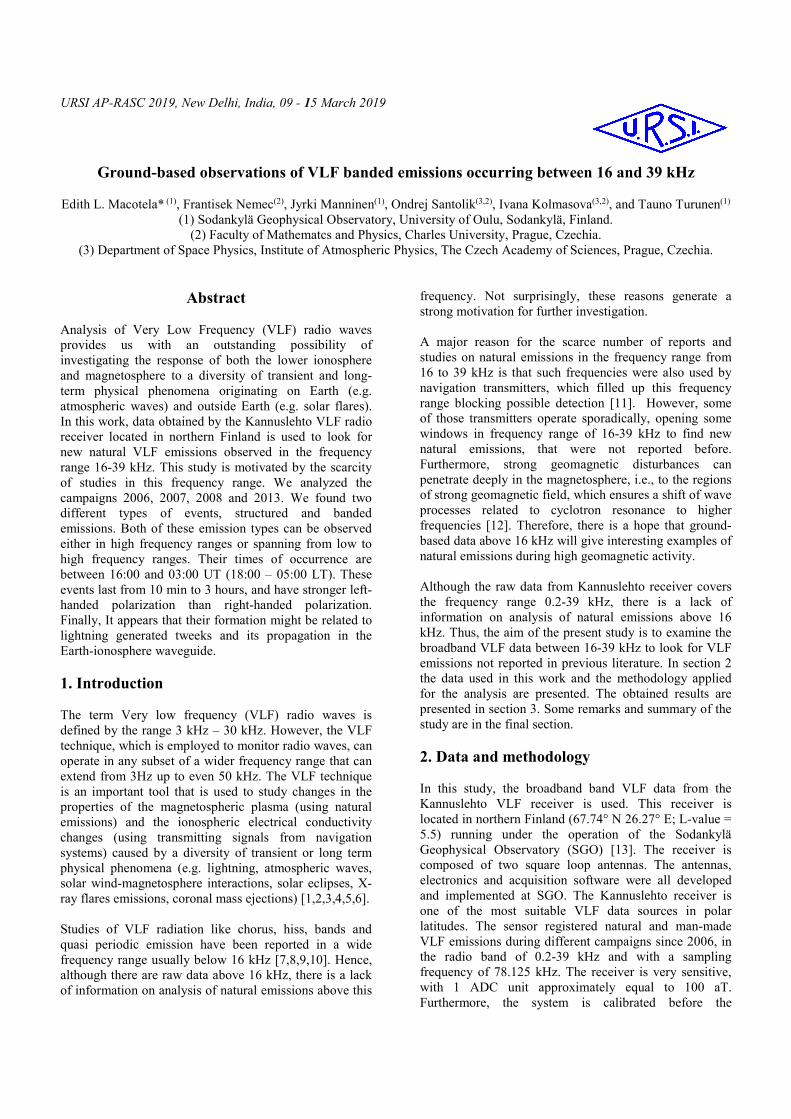
acquisition. All these characteristics make the data very reliable and they are very advantageous even when analyzing weak events. Many naturally occurring VLF waves at frequencies above 4–6 kHz could not be studied in the past because strong atmospherics (sferics) hide all such waves. Sferics originate in lightning discharges [14] and propagate thousands of km in the Earth-ionosphere waveguide. To study the high frequency emissions, we have to apply special digital tools which filter out the strong impulsive sferics. That process uncovers completely new types of high frequency VLF emissions with various unusual spectral structures that have never been seen before. More information about the sferics removal technique can be found in [15]. In this study we use spectrograms after filtering. We also remove the narrowband transmitter signals and Power Line Harmonic Radiations (PLHRs). Figure 1 shows 24-hour total power spectrogram (frequency–time dynamic spectra) for the frequency range 0.2-39 kHz obtained after removing the sferics on 08 December 2013. This figure illustrates an open window of observation for natural emissions below 12 kHz and another window between 26 and 37 kHz. The signals from navigation transmitters in the form of horizontal lines essentially prevents the observations at middle frequencies.

Figure 1. A 24 hours dynamic spectrogram for the frequency range 0.2–39 kHz of filtered VLF data recorded on 08 December 2013.

The times employed in the figures showed here are UT. However, we would like to point out that the local time in Finland is calculated according to the Eastern European Summer Time (EEST): +0300 UTC. 3. Results Figures 2 and 3 shows examples of structured VLF emissions obtained on different days. The figures are 1 h

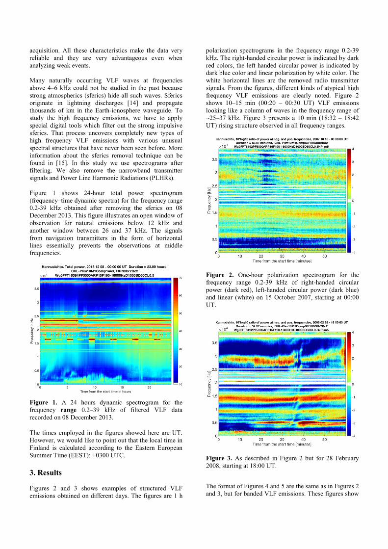
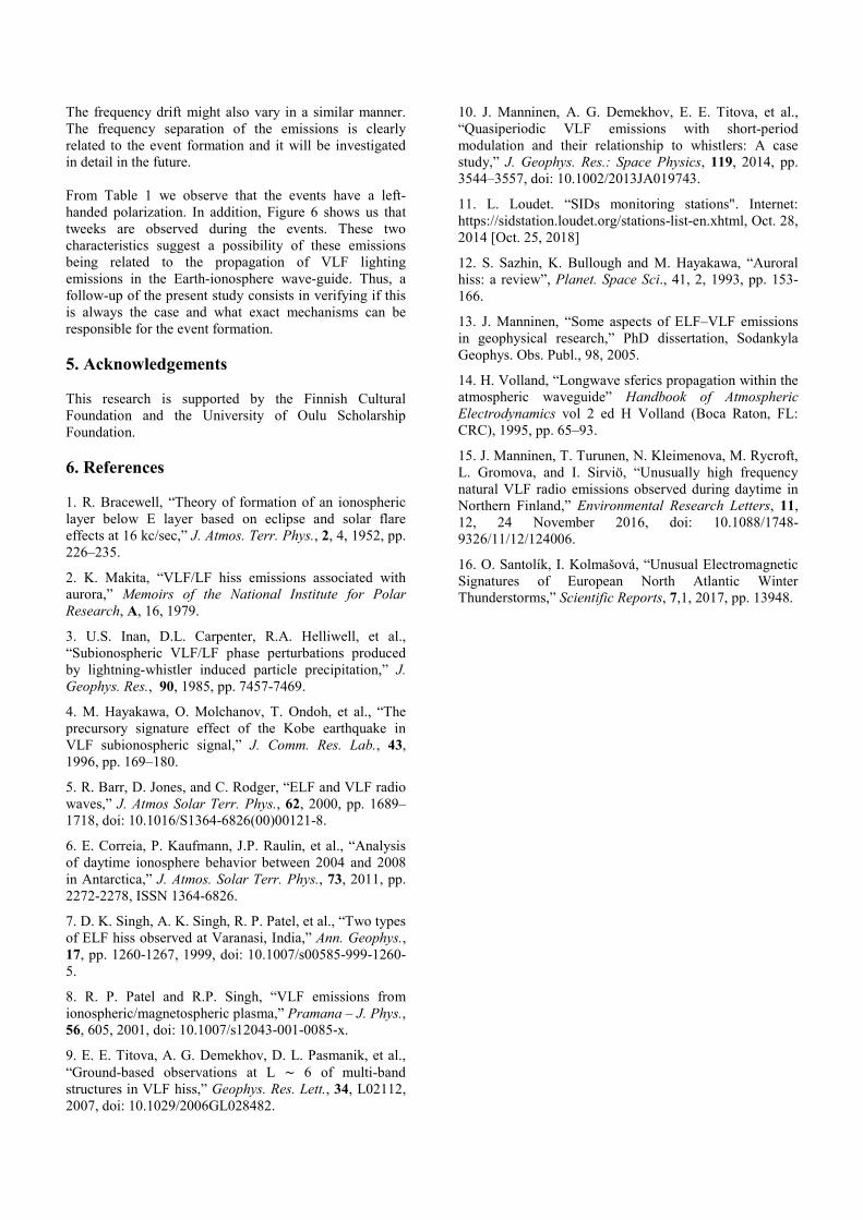
polarization spectrograms in the frequency range 0.2-39 kHz. The right-handed circular power is indicated by dark red colors, the left-handed circular power is indicated by dark blue color and linear polarization by white color. The white horizontal lines are the removed radio transmitter signals. From the figures, different kinds of atypical high frequency VLF emissions are clearly noted. Figure 2 shows 10–15 min (00:20 – 00:30 UT) VLF emissions looking like a column of waves in the frequency range of ~25–37 kHz. Figure 3 presents a 10 min (18:32 – 18:42 UT) rising structure observed in all frequency ranges.

Figure 2. One-hour polarization spectrogram for the frequency range 0.2-39 kHz of right-handed circular power (dark red), left-handed circular power (dark blue) and linear (white) on 15 October 2007, starting at 00:00 UT.

Figure 3. As described in Figure 2 but for 28 February 2008, starting at 18:00 UT.

The format of Figures 4 and 5 are the same as in Figures 2 and 3, but for banded VLF emissions. These figures show

different kinds of atypical high frequency banded VLF emissions. Figure 4 shows 40 min (17:40 – 18:20 UT) of banded emissions in the frequency range of ~25–37 kHz. Figure 5 presents a 1 hour (18:00 – 19:00 UT) of banded emissions observed in all frequency ranges. VLF auroral hiss emissions are also observed at the time in which the banded emissions are occurring. Surprisingly, a change in polarization, from right-handed to left-handed is observed in Figure 4 at about minute 18:23 UT.

Figure 4. As described in Figure 2 but for 24 November 2006, starting at 17:30 UT.

Figure 5. As described in Figure 2 but for 20 December 2013, starting at 18:00 UT.

Table 1 shows the types and number of natural emissions observed at Kannuslehto at frequencies above 16 kHz. In this table, the behavior of those emission is characterized, i.e. the observed time of occurrence, the polarization and duration of the events. The events have primarily a left-handed polarization, and are observed in the evening and nighttime hours

Table 1. Classification and behaviour of the selected events.

Campaigns 2006, 2007, 2008, 2013 Types Structured Banded Total events 12 15 Time of occurrence

16:00 – 03:00 UT

16:00 – 21:00 UT

Primary polarization

Left-handed Left-handed

Duration 15 – 180 min 10 – 180 min

We investigated the events for a possible presence of fine internal structures, i.e., observation of a dispersed type of sferics (so called tweek atmospherics or tweeks) because dispersed parts of tweeks are left-handed polarized [16]. For that we use recordings around the middle time of the event. Figure 6 shows 5-second total power frequency–time dynamic spectra for the frequency range 0.2-39 kHz recorded on 22 November 2006. The white and blue horizontal lines are the removed radio transmitter signals. This figure reveals tweeks, suggesting the possibility of the observed events being related to the propagation of VLF lighting emissions in the Earth-ionosphere wave-guide.

Figure 6. 5-second dynamic spectrogram for the frequency range 0.2–39 kHz of filtered VLF data recorded on 22 November 2006, starting at 19:16 UT.

4. Remarks and Summary In this study, VLF natural emissions observed in high frequency ranges are used. From Figures 2, 3, 4 and 5 we notice that some of the emissions are only observed in high frequency ranges (25-37 kHz), while others are observed in all the frequencies recorded at Kannuslehto (0.2-39 kHz). In the case of the banded emissions, the figures suggest that the band separation is not constant, but it may vary both as a function of time and frequency.

The frequency drift might also vary in a similar manner. The frequency separation of the emissions is clearly related to the event formation and it will be investigated in detail in the future. From Table 1 we observe that the events have a left-handed polarization. In addition, Figure 6 shows us that tweeks are observed during the events. These two characteristics suggest a possibility of these emissions being related to the propagation of VLF lighting emissions in the Earth-ionosphere wave-guide. Thus, a follow-up of the present study consists in verifying if this is always the case and what exact mechanisms can be responsible for the event formation. 5. Acknowledgements This research is supported by the Finnish Cultural Foundation and the University of Oulu Scholarship Foundation. 6. References 1. R. Bracewell, “Theory of formation of an ionospheric layer below E layer based on eclipse and solar flare effects at 16 kc/sec,” J. Atmos. Terr. Phys., 2, 4, 1952, pp. 226–235.

2. K. Makita, “VLF/LF hiss emissions associated with aurora,” Memoirs of the National Institute for Polar Research, A, 16, 1979.

3. U.S. Inan, D.L. Carpenter, R.A. Helliwell, et al., “Subionospheric VLF/LF phase perturbations produced by lightning-whistler induced particle precipitation,” J. Geophys. Res., 90, 1985, pp. 7457-7469.

4. M. Hayakawa, O. Molchanov, T. Ondoh, et al., “The precursory signature effect of the Kobe earthquake in VLF subionospheric signal,” J. Comm. Res. Lab., 43, 1996, pp. 169–180.

5. R. Barr, D. Jones, and C. Rodger, “ELF and VLF radio waves,” J. Atmos Solar Terr. Phys., 62, 2000, pp. 1689–1718, doi: 10.1016/S1364-6826(00)00121-8.

6. E. Correia, P. Kaufmann, J.P. Raulin, et al., “Analysis of daytime ionosphere behavior between 2004 and 2008 in Antarctica,” J. Atmos. Solar Terr. Phys., 73, 2011, pp. 2272-2278, ISSN 1364-6826.

7. D. K. Singh, A. K. Singh, R. P. Patel, et al., “Two types of ELF hiss observed at Varanasi, India,” Ann. Geophys., 17, pp. 1260-1267, 1999, doi: 10.1007/s00585-999-1260-5.

8. R. P. Patel and R.P. Singh, “VLF emissions from ionospheric/magnetospheric plasma,” Pramana – J. Phys., 56, 605, 2001, doi: 10.1007/s12043-001-0085-x.

9. E. E. Titova, A. G. Demekhov, D. L. Pasmanik, et al., “Ground-based observations at L ∼ 6 of multi-band structures in VLF hiss,” Geophys. Res. Lett., 34, L02112, 2007, doi: 10.1029/2006GL028482.

10. J. Manninen, A. G. Demekhov, E. E. Titova, et al., “Quasiperiodic VLF emissions with short-period modulation and their relationship to whistlers: A case study,” J. Geophys. Res.: Space Physics, 119, 2014, pp. 3544–3557, doi: 10.1002/2013JA019743.

11. L. Loudet. “SIDs monitoring stations". Internet: https://sidstation.loudet.org/stations-list-en.xhtml, Oct. 28, 2014 [Oct. 25, 2018]

12. S. Sazhin, K. Bullough and M. Hayakawa, “Auroral hiss: a review”, Planet. Space Sci., 41, 2, 1993, pp. 153-166.

13. J. Manninen, “Some aspects of ELF–VLF emissions in geophysical research,” PhD dissertation, Sodankyla Geophys. Obs. Publ., 98, 2005.

14. H. Volland, “Longwave sferics propagation within the atmospheric waveguide” Handbook of Atmospheric Electrodynamics vol 2 ed H Volland (Boca Raton, FL: CRC), 1995, pp. 65–93.

15. J. Manninen, T. Turunen, N. Kleimenova, M. Rycroft, L. Gromova, and I. Sirviö, “Unusually high frequency natural VLF radio emissions observed during daytime in Northern Finland,” Environmental Research Letters, 11, 12, 24 November 2016, doi: 10.1088/1748-9326/11/12/124006.

16. O. Santolík, I. Kolmašová, “Unusual Electromagnetic Signatures of European North Atlantic Winter Thunderstorms,” Scientific Reports, 7,1, 2017, pp. 13948.