
GUIDE User Manual∗
(updated for version 27.9)
Wei-Yin LohDepartment of Statistics
University of Wisconsin–Madison
April 2, 2018
Contents
1 Warranty disclaimer 4
2 Introduction 52.1 Installation . . . . . . . . . . . . . . . . . . . . . . . . . . . . . . . . 62.2 LATEX . . . . . . . . . . . . . . . . . . . . . . . . . . . . . . . . . . . 8
3 Program operation 93.1 Required files . . . . . . . . . . . . . . . . . . . . . . . . . . . . . . . 93.2 Input file creation . . . . . . . . . . . . . . . . . . . . . . . . . . . . . 12
4 Classification 134.1 Univariate splits, ordinal predictors: glaucoma data . . . . . . . . . . 13
4.1.1 Input file generation . . . . . . . . . . . . . . . . . . . . . . . 134.1.2 Contents of glaucoma.in . . . . . . . . . . . . . . . . . . . . 154.1.3 Executing the program . . . . . . . . . . . . . . . . . . . . . . 164.1.4 Interpreting the output file . . . . . . . . . . . . . . . . . . . . 18
4.2 Linear splits: glaucoma data . . . . . . . . . . . . . . . . . . . . . . . 26
∗Based on work partially supported by grants from the U.S. Army Research Office, NationalScience Foundation, National Institutes of Health, Bureau of Labor Statistics, and Eli Lilly & Co.Work on precursors to GUIDE additionally supported by IBM and Pfizer.
1

CONTENTS CONTENTS
4.3 Univariate splits, categorical predictors: peptide data . . . . . . . . . 304.3.1 Input file generation . . . . . . . . . . . . . . . . . . . . . . . 304.3.2 Results . . . . . . . . . . . . . . . . . . . . . . . . . . . . . . . 31
4.4 Unbalanced classes and equal priors: hepatitis data . . . . . . . . . . 354.5 Unequal misclassification costs: hepatitis data . . . . . . . . . . . . . 394.6 More than 2 classes: dermatology . . . . . . . . . . . . . . . . . . . . 40
4.6.1 Default option . . . . . . . . . . . . . . . . . . . . . . . . . . . 404.6.2 Nearest-neighbor option . . . . . . . . . . . . . . . . . . . . . 494.6.3 Kernel density option . . . . . . . . . . . . . . . . . . . . . . . 58
4.7 More than 2 classes: heart disease . . . . . . . . . . . . . . . . . . . . 684.7.1 Input file creation . . . . . . . . . . . . . . . . . . . . . . . . . 684.7.2 Results . . . . . . . . . . . . . . . . . . . . . . . . . . . . . . . 734.7.3 RPART model . . . . . . . . . . . . . . . . . . . . . . . . . . 90
5 Regression 925.1 Least squares constant: birthwt data . . . . . . . . . . . . . . . . . . 92
5.1.1 Input file creation . . . . . . . . . . . . . . . . . . . . . . . . . 925.1.2 Results . . . . . . . . . . . . . . . . . . . . . . . . . . . . . . . 955.1.3 Contents of cons.var . . . . . . . . . . . . . . . . . . . . . . 107
5.2 Least squares simple linear: birthwt data . . . . . . . . . . . . . . . . 1085.2.1 Input file creation . . . . . . . . . . . . . . . . . . . . . . . . . 1085.2.2 Results . . . . . . . . . . . . . . . . . . . . . . . . . . . . . . . 1115.2.3 Contents of lin.var . . . . . . . . . . . . . . . . . . . . . . . 1155.2.4 Contents of lin.reg . . . . . . . . . . . . . . . . . . . . . . . 116
5.3 Multiple linear: birthwt data . . . . . . . . . . . . . . . . . . . . . . . 1165.3.1 Input file creation . . . . . . . . . . . . . . . . . . . . . . . . . 1165.3.2 Results . . . . . . . . . . . . . . . . . . . . . . . . . . . . . . . 1195.3.3 Contents of mul.var . . . . . . . . . . . . . . . . . . . . . . . 1235.3.4 Contents of mul.reg . . . . . . . . . . . . . . . . . . . . . . . 123
5.4 Stepwise linear: birthwt data . . . . . . . . . . . . . . . . . . . . . . 1245.4.1 Input file creation . . . . . . . . . . . . . . . . . . . . . . . . . 1245.4.2 Contents of step.reg . . . . . . . . . . . . . . . . . . . . . . 125
5.5 Best ANCOVA: birthwt data . . . . . . . . . . . . . . . . . . . . . . 1265.5.1 Input file creation . . . . . . . . . . . . . . . . . . . . . . . . . 1265.5.2 Results . . . . . . . . . . . . . . . . . . . . . . . . . . . . . . . 1295.5.3 Contents of ancova.reg . . . . . . . . . . . . . . . . . . . . . 132
5.6 Quantile regression: birthwt data . . . . . . . . . . . . . . . . . . . . 1325.6.1 Piecewise constant: 1 quantile . . . . . . . . . . . . . . . . . . 133
Wei-Yin Loh 2 GUIDE manual

CONTENTS CONTENTS
5.6.2 Input file creation . . . . . . . . . . . . . . . . . . . . . . . . . 1335.6.3 Results . . . . . . . . . . . . . . . . . . . . . . . . . . . . . . . 1345.6.4 Piecewise constant: 2 quantiles . . . . . . . . . . . . . . . . . 1405.6.5 Input file creation . . . . . . . . . . . . . . . . . . . . . . . . . 1405.6.6 Results . . . . . . . . . . . . . . . . . . . . . . . . . . . . . . . 1435.6.7 Piecewise simple linear . . . . . . . . . . . . . . . . . . . . . . 1505.6.8 Input file creation . . . . . . . . . . . . . . . . . . . . . . . . . 1505.6.9 Results . . . . . . . . . . . . . . . . . . . . . . . . . . . . . . . 1535.6.10 Piecewise multiple linear . . . . . . . . . . . . . . . . . . . . . 1565.6.11 Input file creation . . . . . . . . . . . . . . . . . . . . . . . . . 1585.6.12 Results . . . . . . . . . . . . . . . . . . . . . . . . . . . . . . . 159
5.7 Least median of squares: birthwt data . . . . . . . . . . . . . . . . . 1625.7.1 Results . . . . . . . . . . . . . . . . . . . . . . . . . . . . . . . 165
5.8 Poisson regression with offset: lung cancer data . . . . . . . . . . . . 1705.8.1 Input file creation . . . . . . . . . . . . . . . . . . . . . . . . . 1725.8.2 Results . . . . . . . . . . . . . . . . . . . . . . . . . . . . . . . 173
5.9 Censored response: heart attack data . . . . . . . . . . . . . . . . . . 1775.9.1 Results . . . . . . . . . . . . . . . . . . . . . . . . . . . . . . . 180
5.10 Multi-response: public health data . . . . . . . . . . . . . . . . . . . 1865.10.1 Input file creation . . . . . . . . . . . . . . . . . . . . . . . . . 1875.10.2 Results . . . . . . . . . . . . . . . . . . . . . . . . . . . . . . . 190
5.11 Longitudinal response with varying time: wage data . . . . . . . . . . 1935.11.1 Input file creation . . . . . . . . . . . . . . . . . . . . . . . . . 1955.11.2 Results . . . . . . . . . . . . . . . . . . . . . . . . . . . . . . . 198
5.12 Subgroup identification: breast cancer . . . . . . . . . . . . . . . . . 2045.12.1 Without linear prognostic control . . . . . . . . . . . . . . . . 2055.12.2 Simple linear prognostic control . . . . . . . . . . . . . . . . . 2145.12.3 Multiple linear prognostic control . . . . . . . . . . . . . . . . 218
6 Importance scoring 2236.1 Classification: glaucoma data . . . . . . . . . . . . . . . . . . . . . . 223
6.1.1 Input file creation . . . . . . . . . . . . . . . . . . . . . . . . . 2236.1.2 Contents of imp.out . . . . . . . . . . . . . . . . . . . . . . . 224
6.2 Regression with censoring: heart attack data . . . . . . . . . . . . . . 226
7 Differential item functioning: GDS data 235
Wei-Yin Loh 3 GUIDE manual

1 WARRANTY DISCLAIMER
8 Tree ensembles 2388.1 GUIDE forest: hepatitis data . . . . . . . . . . . . . . . . . . . . . . 2398.2 Input file creation . . . . . . . . . . . . . . . . . . . . . . . . . . . . . 2398.3 Results . . . . . . . . . . . . . . . . . . . . . . . . . . . . . . . . . . . 2408.4 Bagged GUIDE . . . . . . . . . . . . . . . . . . . . . . . . . . . . . . 243
9 Other features 2469.1 Pruning with test samples . . . . . . . . . . . . . . . . . . . . . . . . 2469.2 Prediction of test samples . . . . . . . . . . . . . . . . . . . . . . . . 2479.3 GUIDE in R and in simulations . . . . . . . . . . . . . . . . . . . . . 2479.4 Generation of powers and products . . . . . . . . . . . . . . . . . . . 2489.5 Data formatting functions . . . . . . . . . . . . . . . . . . . . . . . . 249
1 Warranty disclaimer
Redistribution and use in binary forms, with or without modification, are permittedprovided that the following condition is met:
Redistributions in binary form must reproduce the above copyright notice, thiscondition and the following disclaimer in the documentation and/or other materialsprovided with the distribution.
THIS SOFTWARE IS PROVIDED BY WEI-YIN LOH “AS IS” AND ANY EX-PRESS OR IMPLIED WARRANTIES, INCLUDING, BUT NOT LIMITED TO,THE IMPLIED WARRANTIES OF MERCHANTABILITY AND FITNESS FOR APARTICULAR PURPOSE ARE DISCLAIMED. IN NO EVENT SHALL WEI-YINLOH BE LIABLE FOR ANY DIRECT, INDIRECT, INCIDENTAL, SPECIAL, EX-EMPLARY, OR CONSEQUENTIAL DAMAGES (INCLUDING, BUT NOT LIM-ITED TO, PROCUREMENT OF SUBSTITUTE GOODS OR SERVICES; LOSSOF USE, DATA, OR PROFITS; OR BUSINESS INTERRUPTION) HOWEVERCAUSED AND ON ANY THEORY OF LIABILITY, WHETHER IN CONTRACT,STRICT LIABILITY, OR TORT (INCLUDING NEGLIGENCE OR OTHERWISE)ARISING IN ANY WAY OUT OF THE USE OF THIS SOFTWARE, EVEN IFADVISED OF THE POSSIBILITY OF SUCH DAMAGE.
The views and conclusions contained in the software and documentation are thoseof the author and should not be interpreted as representing official policies, eitherexpressed or implied, of the University of Wisconsin.
Wei-Yin Loh 4 GUIDE manual

2 INTRODUCTION
2 Introduction
GUIDE stands for Generalized, Unbiased, Interaction Detection and Estimation. It isan algorithm for construction of classification and regression trees and forests. It is adescendent of the FACT (Loh and Vanichsetakul, 1988), SUPPORT (Chaudhuri et al.,1994, 1995), QUEST (Loh and Shih, 1997), CRUISE (Kim and Loh, 2001, 2003), andLOTUS (Chan and Loh, 2004; Loh, 2006a) algorithms. GUIDE is the only classifi-cation and regression tree algorithm with all these features:
1. Unbiased variable selection.
2. Automatic handling of missing values without requiring prior imputation.
3. Kernel and nearest-neighbor node models for classification trees.
4. Weighted least squares, least median of squares, quantile, Poisson, and relativerisk (proportional hazards) regression models.
5. Univariate, multivariate, censored, and longitudinal response variables.
6. Pairwise interaction detection at each node.
7. Linear splits on two variables at a time for classification trees.
8. Categorical variables for splitting only, or for both splitting and fitting (via 0-1dummy variables), in regression tree models.
9. Ranking and scoring of predictor variables.
10. Tree ensembles (bagging and forests).
11. Subgroup identification for differential treatment effects.
Tables 1 and 2 compare the features of GUIDE with QUEST, CRUISE, C4.5 (Quinlan,1993), RPART (Therneau et al., 2017) 1, and M5’ (Quinlan, 1992; Witten and Frank,2000).
The GUIDE algorithm is documented in Loh (2002) for regression trees and Loh(2009) for classification trees. Reviews of the subject may be found in Loh (2008a),Loh (2011) and Loh (2014). Some advanced features of the algorithm are reportedin Chaudhuri and Loh (2002), Loh (2006b), Kim et al. (2007), Loh et al. (2007),
1RPART is an implementation of CART (Breiman et al., 1984) in R. CART is a registeredtrademark of California Statistical Software, Inc.
Wei-Yin Loh 5 GUIDE manual

2.1 Installation 2 INTRODUCTION
Table 1: Comparison of GUIDE, QUEST, CRUISE, CART, and C4.5 classificationtree algorithms. Node models: S = simple, K = kernel, L = linear discriminant, N =nearest-neighbor.
GUIDE QUEST CRUISE CART C4.5Unbiased splits Yes Yes Yes No NoSplits per node 2 2 ≥ 2 2 2Interactiondetection
Yes No Yes No No
Importanceranking
Yes No No Yes No
Class priors Yes Yes Yes Yes NoMisclassificationcosts
Yes Yes Yes Yes No
Linear splits Yes Yes Yes Yes NoCategoricalsplits
Subsets Subsets Subsets Subsets Atoms
Node models S, K, N S S, L S SMissing values Special Imputation Surrogate Surrogate WeightsTree diagrams Text and LATEX Proprietary TextBagging Yes No No No NoForests Yes No No No No
and Loh (2008b). A list of third-party applications of GUIDE, CRUISE, QUEST,and LOTUS is maintained in http://www.stat.wisc.edu/~loh/apps.html. Thismanual illustrates the use of the GUIDE software and the interpretation of theoutput.
2.1 Installation
GUIDE is available free from www.stat.wisc.edu/~loh/guide.html in the form ofcompiled 32- and 64-bit executables for Linux, Mac OS X, and Windows on Inteland compatible processors. Data and description files used in this manual are in thezip file www.stat.wisc.edu/~loh/treeprogs/guide/datafiles.zip.
Linux: There are three 64-bit executables to choose from: Intel and NAG (for RedHat 6.8), and Gfortran (for Ubuntu 16.0). Make the unzipped file executableby issuing this command in a Terminal application in the folder where the file
Wei-Yin Loh 6 GUIDE manual

2.1 Installation 2 INTRODUCTION
Table 2: Comparison of GUIDE, CART and M5’ regression tree algorithms
GUIDE CART M5’Unbiased splits Yes No NoPairwise interac-tion detection
Yes No No
Importance scores Yes Yes NoLoss functions Weighted least squares, least
median of squares, quantile,Poisson, proportional hazards
Least squares,least absolutedeviations
Least squaresonly
Survival, longitu-dinal and multi-response data
Yes, yes, yes No, no, no No, no, no
Node models Constant, multiple, stepwiselinear, polynomial, ANCOVA
Constant only Constant andstepwise
Linear models Multiple or stepwise (forwardand forward-backward)
N/A Stepwise
Variable roles Split only, fit only, both, nei-ther, weight, censored, offset
Split only Split and fit
Categorical vari-able splits
Subsets of categorical values Subsets 0-1 variables
Tree selection Pruning or stopping rules Pruning only Pruning onlyTree diagrams Text and LATEX Proprietary PostScriptOperation modes Batch Interactive
and batchInteractive
Case weights Yes Yes NoTransformations Powers and products No NoMissing values insplit variables
Missing values treated as aspecial category
Surrogatesplits
Imputation
Missing values inlinear predictors
Choice of separate constantmodels or mean imputation
N/A Imputation
Bagging & forests Yes & yes No & no No & noSubgroup identifi-cation
Yes No No
Data conversions ARFF, C4.5, Minitab, R,SAS, Statistica, Systat, CSV
No No
Wei-Yin Loh 7 GUIDE manual

2.2 LATEX 2 INTRODUCTION
is located: chmod a+x guide.
Mac OS X: There are three executables to choose from. Make the unzipped fileexecutable by issuing this command in a Terminal application in the folderwhere the file is located: chmod a+x guide
NAG. This version may be the fastest. It requires no additional softwarebesides the guide.gz file.
Absoft. This version requires no additional software besides the guide.gz filetoo.
Gfortran. This version requires Xcode and gfortran to be installed. Toensure that the gfortran libraries are placed in the right place, followthese steps:
1. InstallXcode from https://developer.apple.com/xcode/downloads/.
2. Go to http://hpc.sourceforge.net and download file gcc-7.1-bin.tar.gzto your Downloads folder. The direct link to the file ishttp://prdownloads.sourceforge.net/hpc/gcc-7.1-bin.tar.gz?download
3. Open a Terminal window and type (or copy and paste):
(a) cd ~/Downloads
(b) gunzip gcc-7.1-bin.tar.gz
(c) sudo tar -xvf gcc-7.1-bin.tar -C /
Windows: There are four executables to choose from: Intel (64 or 32 bit), Absoft(64 bit) and Gfortran (64 bit). The 32-bit executable may run a bit fasterbut the 64-bit versions can handle larger arrays. Download the 32 or 64-bitexecutable guide.zip and unzip it (right-click on file icon and select “Extractall”). The resulting file guide.exe may be placed in one of three places:
1. top level of your C: drive (where it can be invoked by typing C:\guide ina terminal window—see Section 3.1),
2. a folder that contains your data files, or
3. a folder on your search path.
2.2 LATEX
GUIDE uses the public-domain software LATEX (http://www.ctan.org) to producetree diagrams. The specific locations are:
Wei-Yin Loh 8 GUIDE manual

3 PROGRAM OPERATION
Linux: TeX Live http://www.tug.org/texlive/
Mac: MacTeX http://tug.org/mactex/
Windows: proTeXt http://www.tug.org/protext/
After LATEX is installed, a pdf file of a LATEX file, called diagram.tex say, producedby GUIDE can be obtained by typing these three commands in a terminal window:
1. latex diagram
2. dvips diagram
3. ps2pdf diagram.ps
The first command produces a file called diagram.dvi which the second com-mand uses to create a postscript file called diagram.ps. The latter can be viewedand printed if a postscript viewer (such as Preview for the Mac) is installed. Ifno postscript viewer is available, the last command can be used to convert thepostscript file into a pdf file, which can be viewed and printed with Adobe Reader.The file diagram.tex can be edited to change colors, node sizes, etc. See, e.g.,http://tug.org/PSTricks/main.cgi/.
Windows users: Convert the postscript figure to Enhanced-format Meta File(emf) format for use in Windows applications such as Word or PowerPoint. Thereare many conversion programs are available on the web, such as Graphic Converter(http://www.graphic-converter.net/) and pstoedit (http://www.pstoedit.net/).
3 Program operation
3.1 Required files
The GUIDE program requires two text files for input.
Data file: This file contains the training sample. Each file record consists of ob-servations on the response (i.e., dependent) variable, the predictor (i.e., X orindependent) variables, and optional weight and time variables. Entries in eachrecord are comma, space, or tab delimited (multiple spaces are treated as onespace, but not for commas). A record can occupy more than one line in thefile, but each record must begin on a new line.
Values of categorical variables can contain any ascii character except singleand double quotation marks, which are used to enclose values that contain
Wei-Yin Loh 9 GUIDE manual
3.1 Required files 3 PROGRAM OPERATION
spaces and commas. Values can be up to 60 characters long. Class labels aretruncated to 10 characters in tabular displays.
A common problem among first-time users is getting the data file in propershape. If the data are in a spreadsheet and there are no empty cells, exportthem to a MS-DOS Comma Separated (csv) file (the MS-DOS CSV formattakes care of carriage return and line feed characters properly). If there areempty cells, a good solution is to read the spreadsheet into R (using read.csv
with proper specification of the na.strings argument), verify that the data arecorrectly read, and then export them to a text file using either write.tableor write.csv.
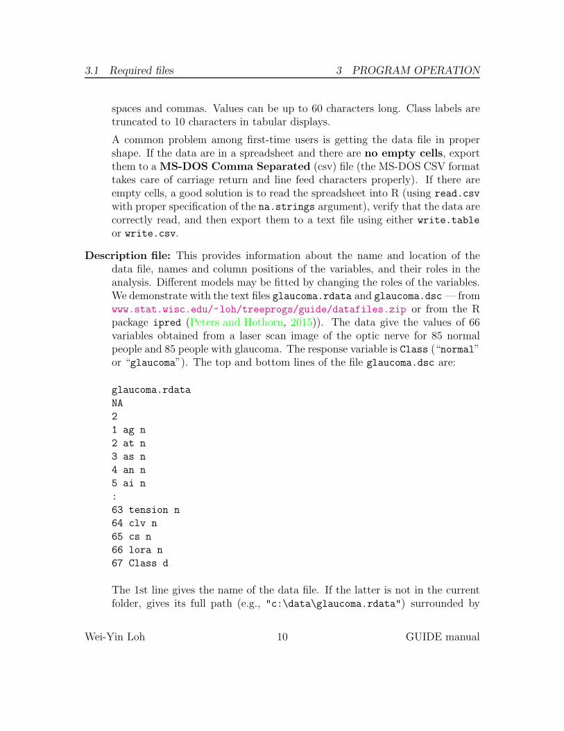
Description file: This provides information about the name and location of thedata file, names and column positions of the variables, and their roles in theanalysis. Different models may be fitted by changing the roles of the variables.We demonstrate with the text files glaucoma.rdata and glaucoma.dsc — fromwww.stat.wisc.edu/~loh/treeprogs/guide/datafiles.zip or from the Rpackage ipred (Peters and Hothorn, 2015)). The data give the values of 66variables obtained from a laser scan image of the optic nerve for 85 normalpeople and 85 people with glaucoma. The response variable is Class (“normal”or “glaucoma”). The top and bottom lines of the file glaucoma.dsc are:
glaucoma.rdata
NA
2
1 ag n
2 at n
3 as n
4 an n
5 ai n
:
63 tension n
64 clv n
65 cs n
66 lora n
67 Class d
The 1st line gives the name of the data file. If the latter is not in the currentfolder, gives its full path (e.g., "c:\data\glaucoma.rdata") surrounded by
Wei-Yin Loh 10 GUIDE manual
3.1 Required files 3 PROGRAM OPERATION
quotes (because it contains backslashes). The 2nd line gives the missing valuecode, which can be up to 80 characters long. If it contains non-alphanumericcharacters, it too must be surrounded by quotation marks. A missing valuecode must appear in the second line of the file even if there are no missingvalues in the data (in which case any character string not present among thedata values can be used). The 3rd line gives the line number of the first datarecord in the data file. Because glaucoma.rdata has the variable names in thefirst row, a “2” is placed on the third line of glaucoma.dsc. Blank lines inthe data and description files are ignored. The position, name and role of eachvariable comes next (in that order), with one line for each variable.
Variable names must begin with an alphabet and be not more than 60 charac-ters long. If a name contains non-alphanumeric characters, it must be enclosedin matching single or double quotes. Spaces and the four characters #, %, {,and } are replaced by dots (periods) if they appear in a name. Variable namesare truncated to 10 characters in tabular output. Leading and trailing spacesare dropped.
The following roles for the variables are permitted. Lower and upper caseletters are accepted.
b Categorical variable that is used both for splitting and for node modeling inregression. It is transformed to 0-1 dummy variables for node modeling.It is converted to c type for classification.
c Categorical variable used for splitting only.
d Dependent variable. Except for multi-response data (see Sec. 5.10), therecan only be one such variable. In the case of relative risk models, thisis the death indicator. The variable can take character string values forclassification.
f Numerical variable used only for f itting the linear models in the nodes of thetree. It is not used for splitting the nodes and is disallowed in classification.
n Numerical variable used both for splitting the nodes and for fitting the nodemodels. It is converted to type s in classification.
r Categorical treatment (Rx) variable used only for fitting the linear modelsin the nodes of the tree. It is not used for splitting the nodes. If thisvariable is present, all n variables are automatically changed to s.
s Numerical-valued variable only used for splitting the nodes. It is not used asa regressor in the linear models. This role is suitable for ordinal categoricalvariables if they are given numerical values that reflect the orderings.
Wei-Yin Loh 11 GUIDE manual

3.2 Input file creation 3 PROGRAM OPERATION
t Survival time (for proportional hazards models) or observation time (forlongitudinal models) variable.
w Weight variable for weighted least squares regression or for excluding ob-servations in the training sample from tree construction. See section 9.2for the latter. Except for longitudinal models, a record with a missingvalue in a d, t, or z-variable is automatically assigned zero weight.
x Excluded variable. This allows models to be fitted to different subsets ofthe variables without reformatting the data file.
z Offset variable used only in Poisson regression.
GUIDE runs within a terminal window of the computer operating system.
Do not double-click its icon on the desktop!
Linux. Any terminal program will do.
Mac OS X. The program is called Terminal; it is in the Applications Folder.
Windows. The terminal program is started from the Start button by choosingAll Programs → Accessories → Command Prompt
After the terminal window is opened, change to the folder where the data and pro-gram files are stored. For Windows users who do not know how to do this, readhttp://www.digitalcitizen.life/command-prompt-how-use-basic-commands.
3.2 Input file creation
GUIDE is started by typing its (lowercase) name in a terminal. The preferred wayis to create an input file (option 1 below) for subsequent execution. The input filemay be edited if you wish to change some input parameters later. In the following,the sign (>) is the terminal prompt (not to be typed!).
> guide
GUIDE Classification and Regression Trees and Forests
Version 27.9 (Build date: April 1, 2018)
Compiled with NAG Fortran 6.2.0 on Mac OS X Sierra 10.13.4
Copyright (c) 1997-2018 Wei-Yin Loh. All rights reserved.
This software is based upon work supported by the U.S. Army Research Office,
the National Science Foundation and the National Institutes of Health.
Choose one of the following options:
Wei-Yin Loh 12 GUIDE manual
4 CLASSIFICATION
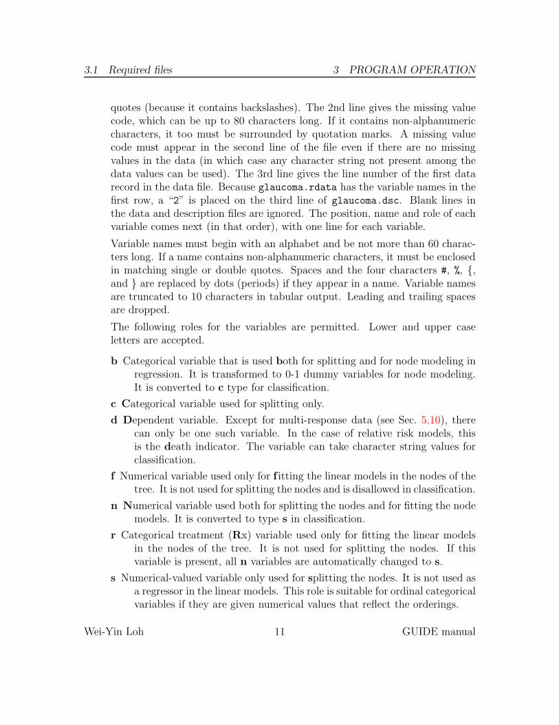
0. Read the warranty disclaimer
1. Create an input file for model fitting or importance scoring (recommended)
2. Convert data to other formats without creating input file
Input your choice:
The meanings of these options are:
0. Print the warranty disclaimer.
1. Create an input file for model fitting or importance scoring (recommended).
2. Convert the data file into a format suitable for importation into database, spread-sheet, or statistics software. See Table 2 for the statistical packages supported.Section 9.5 has an example.
4 Classification
4.1 Univariate splits, ordinal predictors: glaucoma data
We first show how to generate an input file to produce a classification tree fromthe data in the file glaucoma.rdata, using the default options. Whenever you areprompted for a selection, there is usually range of permissible values given withinsquare brackets and a default choice (indicated by the symbol <cr>=). The defaultmay be selected by pressing the ENTER or RETURN key. Annotations are printed inblue italics in this manual.
4.1.1 Input file generation
0. Read the warranty disclaimer
1. Create an input file for model fitting or importance scoring (recommended)
2. Convert data to other formats without creating input file
Input your choice: 1
Name of batch input file: glaucoma.in
This file will store your answers to the prompts.
Input 1 for model fitting, 2 for importance or DIF scoring,
3 for data conversion ([1:3], <cr>=1):
Press the ENTER or RETURN key to accept the default selection.
Name of batch output file: glaucoma.out
This file will contain the results when you apply the input file to GUIDE later.
Input 1 for single tree, 2 for ensemble ([1:2], <cr>=1):
Option 2 is for bagging and random forest-type methods.
Input 1 for classification, 2 for regression, 3 for propensity score grouping
Wei-Yin Loh 13 GUIDE manual

4.1 Univariate splits, ordinal predictors: glaucoma data 4 CLASSIFICATION
(propensity score grouping is an experimental option)
Input your choice ([1:3], <cr>=1):
Input 1 for default options, 2 otherwise ([1:2], <cr>=1):
The default option will produce a traditional classification tree.
Choose option 2 for more advanced features.
Input name of data description file (max 100 characters);
enclose with matching quotes if it has spaces: glaucoma.dsc
Reading data description file ...
Training sample file: glaucoma.rdata
The name of the data set is read from the description file.
Some information about the data are printed in the next few lines.
Missing value code: NA
Records in data file start on line 2
Warning: N variables changed to S
This warning is due to N variables being always used as S in classification.
Dependent variable is Class
Reading data file ...
Number of records in data file: 170
Length of longest data entry: 8
Checking for missing values ...
Total number of cases: 170
Number of classes = 2
Re-checking data ...
Allocating missing value information
Assigning codes to categorical and missing values
Finished checking data
Creating missing value indicators
Rereading data
Class #Cases Proportion
glaucoma 85 0.50000000
normal 85 0.50000000
Total #cases w/ #missing
#cases miss. D ord. vals #X-var #N-var #F-var #S-var #B-var #C-var
170 0 17 0 0 0 66 0 0
No. cases used for training: 170
No. cases excluded due to 0 weight or missing D: 0
Finished reading data file
Choose 1 for estimated priors, 2 for equal priors, 3 for priors from a file
Input 1, 2, or 3 ([1:3], <cr>=1):
See other parts of manual for examples of equal and specified priors.
Choose 1 for unit misclassification costs, 2 to input costs from a file
Input 1 or 2 ([1:2], <cr>=1):
Input 1 for LaTeX tree code, 2 to skip it ([1:2], <cr>=1):
Choose option 2 if you do not want LaTeX code.
Input file name to store LaTeX code (use .tex as suffix): glaucoma.tex
Input 2 to save individual fitted values and node IDs, 1 otherwise ([1:2], <cr>=2):
Wei-Yin Loh 14 GUIDE manual

4.1 Univariate splits, ordinal predictors: glaucoma data 4 CLASSIFICATION
Input name of file to store node ID and fitted value of each case: glaucoma.fit
This file will contain the node number and predicted class for each observation.
Input file is created!
Run GUIDE with the command: guide < glaucoma.in
4.1.2 Contents of glaucoma.in
Here are the contents of the input file:
GUIDE (do not edit this file unless you know what you are doing)
27.9 (version of GUIDE that generated this file)
1 (1=model fitting, 2=importance or DIF scoring, 3=data conversion)
"glaucoma.out" (name of output file)
1 (1=one tree, 2=ensemble)
1 (1=classification, 2=regression, 3=propensity score grouping)
1 (1=simple model, 2=nearest-neighbor, 3=kernel)
1 (0=linear 1st, 1=univariate 1st, 2=skip linear, 3=skip linear and interaction)
1 (1=prune by CV, 2=by test sample, 3=no pruning)
"glaucoma.dsc" (name of data description file)
10 (number of cross-validations)
1 (1=mean-based CV tree, 2=median-based CV tree)
0.500 (SE number for pruning)
1 (1=estimated priors, 2=equal priors, 3=other priors)
1 (1=unit misclassification costs, 2=other)
2 (1=split point from quantiles, 2=use exhaustive search)
1 (1=default max. number of split levels, 2=specify no. in next line)
1 (1=default min. node size, 2=specify min. value in next line)
1 (1=write latex, 2=skip latex)
"glaucoma.tex" (latex file name)
1 (1=vertical tree)
1 (1=include node numbers, 2=exclude)
1 (1=number all nodes, 2=only terminal nodes)
1 (1=color terminal nodes, 2=no colors)
1 (0=#errors, 1=class sizes in nodes, 2=nothing)
1 (1=no storage, 2=store fit and split variables, 3=store split variables and values)
2 (1=do not save fitted values and node IDs, 2=save in a file)
"glaucoma.fit" (file name for fitted values and node IDs)
1 (1=do not write R function, 2=write R function)
GUIDE reads only the first item in each line; the rest of the line is a comment forhuman consumption. It is generally not advisable for the user to edit this file becauseeach question depends on the answers given to previous questions.
Wei-Yin Loh 15 GUIDE manual

4.1 Univariate splits, ordinal predictors: glaucoma data 4 CLASSIFICATION
4.1.3 Executing the program
After the input file is generated, GUIDE can be executed by typing the command“guide < glaucoma.in” at the screen prompt:
> guide < glaucoma.in
This produces the following output to the screen. The alternative command “guide< glaucoma.in > log.txt” sends the screen output to the file log.txt.
GUIDE Classification and Regression Trees and Forests
Version 27.9 (Build date: April 1, 2018)
Compiled with NAG Fortran 6.2.0 on Mac OS X Sierra 10.13.4
Copyright (c) 1997-2018 Wei-Yin Loh. All rights reserved.
This software is based upon work supported by the U.S. Army Research Office,
the National Science Foundation and the National Institutes of Health.
Choose one of the following options:
0. Read the warranty disclaimer
1. Create a GUIDE input file
Input your choice: Batch run with input file
Input 1 for model fitting, 2 for importance or DIF scoring, 3 for data conversion: 1
Input 1 for single tree, 2 for ensemble of trees: 1
Input 1 for classification, 2 for regression, 3 for propensity score grouping
(propensity score grouping is an experimental option)
Input your choice: 1
Input 1 for simple, 2 for nearest-neighbor, 3 for kernel method: 1
Input 0 for linear, interaction and univariate splits (in this order),
1 for univariate, linear and interaction splits (in this order),
2 to skip linear splits,
3 to skip linear and interaction splits: 1
Input 1 to prune by CV, 2 by test sample, 3 for no pruning: 1
Input name of data description file (max 100 characters);
enclose with matching quotes if it has spaces: glaucoma.dsc
Reading data description file ...
Training sample file: glaucoma.rdata
Missing value code: NA
Records in data file start on line 2
Warning: N variables changed to S
Dependent variable is Class
Reading data file ...
Number of records in data file: 170
Length of longest entry in data file: 8
Checking for missing values ...
Wei-Yin Loh 16 GUIDE manual

4.1 Univariate splits, ordinal predictors: glaucoma data 4 CLASSIFICATION
Total number of cases: 170
Number of classes: 2
Re-checking data ...
Allocating missing value information
Assigning codes to categorical and missing values
Data checks complete
Creating missing value indicators
Rereading data
Class #Cases Proportion
glaucoma 85 0.50000000
normal 85 0.50000000
Total #cases w/ #missing
#cases miss. D ord. vals #X-var #N-var #F-var #S-var #B-var #C-var
170 0 17 0 0 0 66 0 0
No. cases used for training: 170
No. cases excluded due to 0 weight or missing D: 0
Finished reading data file
Univariate split highest priority
Interaction and linear splits 2nd and 3rd priorities
Input number of cross-validations: 10
Selected tree is based on mean of CV estimates
Input number of SEs for pruning: 0.5000000000000000
Choose 1 for estimated priors, 2 for equal priors, 3 for priors from a file
Input 1, 2, or 3: 1
Choose 1 for unit misclassification costs, 2 to input costs from a file
Input 1 or 2: 1
Choose a split point selection method for numerical variables:
Choose 1 to use faster method based on sample quantiles
Choose 2 to use exhaustive search
Input 1 or 2: 2
Max. number of split levels: 10
Input 1 for default min. node size,
2 to specify min. value: 1
Input 1 for LaTeX tree code, 2 to skip it: 1
Input file name to store LaTeX code: glaucoma.tex
Input 1 to include node numbers, 2 to omit them: 1
Input 1 to number all nodes, 2 to number leaves only: 1
Input 0 for #errors, 1 for class sizes in nodes, 2 for nothing: 1
You can store the variables and/or values used to split and fit in a file
Choose 1 to skip this step, 2 to store split and fit variables,
3 to store split variables and their values
Input your choice: 1
Input 2 to save fitted values and node IDs; 1 otherwise: 2
File name is glaucoma.fit
Input 2 to write R function for predicting new cases, 1 otherwise: 1
Constructing main tree ...
Wei-Yin Loh 17 GUIDE manual
4.1 Univariate splits, ordinal predictors: glaucoma data 4 CLASSIFICATION
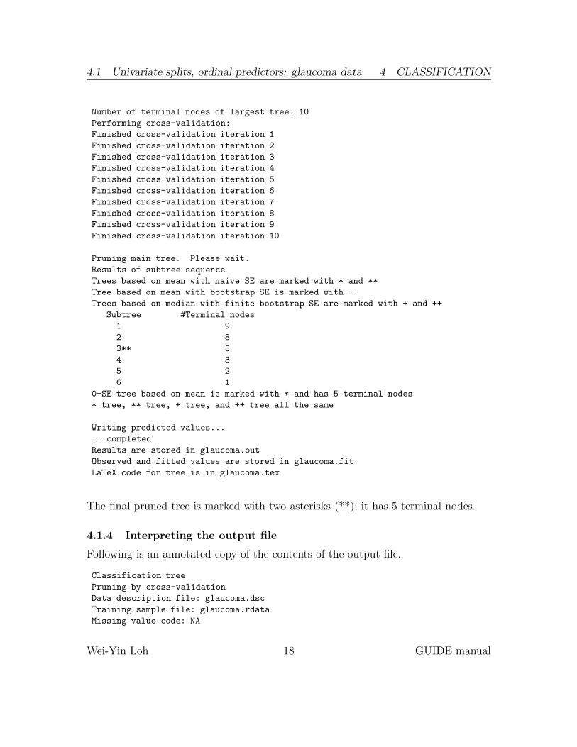
Number of terminal nodes of largest tree: 10
Performing cross-validation:
Finished cross-validation iteration 1
Finished cross-validation iteration 2
Finished cross-validation iteration 3
Finished cross-validation iteration 4
Finished cross-validation iteration 5
Finished cross-validation iteration 6
Finished cross-validation iteration 7
Finished cross-validation iteration 8
Finished cross-validation iteration 9
Finished cross-validation iteration 10
Pruning main tree. Please wait.
Results of subtree sequence
Trees based on mean with naive SE are marked with * and **
Tree based on mean with bootstrap SE is marked with --
Trees based on median with finite bootstrap SE are marked with + and ++
Subtree #Terminal nodes
1 9
2 8
3** 5
4 3
5 2
6 1
0-SE tree based on mean is marked with * and has 5 terminal nodes
* tree, ** tree, + tree, and ++ tree all the same
Writing predicted values...
...completed
Results are stored in glaucoma.out
Observed and fitted values are stored in glaucoma.fit
LaTeX code for tree is in glaucoma.tex
The final pruned tree is marked with two asterisks (**); it has 5 terminal nodes.
4.1.4 Interpreting the output file
Following is an annotated copy of the contents of the output file.
Classification tree
Pruning by cross-validation
Data description file: glaucoma.dsc
Training sample file: glaucoma.rdata
Missing value code: NA
Wei-Yin Loh 18 GUIDE manual
4.1 Univariate splits, ordinal predictors: glaucoma data 4 CLASSIFICATION
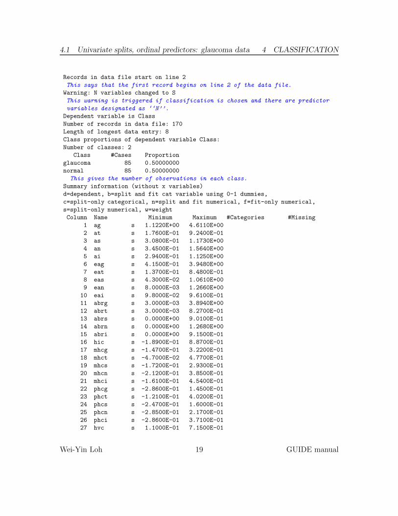
Records in data file start on line 2
This says that the first record begins on line 2 of the data file.
Warning: N variables changed to S
This warning is triggered if classification is chosen and there are predictor
variables designated as ‘‘N’’.
Dependent variable is Class
Number of records in data file: 170
Length of longest data entry: 8
Class proportions of dependent variable Class:
Number of classes: 2
Class #Cases Proportion
glaucoma 85 0.50000000
normal 85 0.50000000
This gives the number of observations in each class.
Summary information (without x variables)
d=dependent, b=split and fit cat variable using 0-1 dummies,
c=split-only categorical, n=split and fit numerical, f=fit-only numerical,
s=split-only numerical, w=weight
Column Name Minimum Maximum #Categories #Missing
1 ag s 1.1220E+00 4.6110E+00
2 at s 1.7600E-01 9.2400E-01
3 as s 3.0800E-01 1.1730E+00
4 an s 3.4500E-01 1.5640E+00
5 ai s 2.9400E-01 1.1250E+00
6 eag s 4.1500E-01 3.9480E+00
7 eat s 1.3700E-01 8.4800E-01
8 eas s 4.3000E-02 1.0610E+00
9 ean s 8.0000E-03 1.2660E+00
10 eai s 9.8000E-02 9.6100E-01
11 abrg s 3.0000E-03 3.8940E+00
12 abrt s 3.0000E-03 8.2700E-01
13 abrs s 0.0000E+00 9.0100E-01
14 abrn s 0.0000E+00 1.2680E+00
15 abri s 0.0000E+00 9.1500E-01
16 hic s -1.8900E-01 8.8700E-01
17 mhcg s -1.4700E-01 3.2200E-01
18 mhct s -4.7000E-02 4.7700E-01
19 mhcs s -1.7200E-01 2.9300E-01
20 mhcn s -2.1200E-01 3.8500E-01
21 mhci s -1.6100E-01 4.5400E-01
22 phcg s -2.8600E-01 1.4500E-01
23 phct s -1.2100E-01 4.0200E-01
24 phcs s -2.4700E-01 1.6000E-01
25 phcn s -2.8500E-01 2.1700E-01
26 phci s -2.8600E-01 3.7100E-01
27 hvc s 1.1000E-01 7.1500E-01
Wei-Yin Loh 19 GUIDE manual

4.1 Univariate splits, ordinal predictors: glaucoma data 4 CLASSIFICATION
28 vbsg s 2.0000E-02 2.0770E+00
29 vbst s 7.0000E-03 4.4600E-01
30 vbss s 2.0000E-03 5.5400E-01
31 vbsn s 0.0000E+00 6.9600E-01
32 vbsi s 6.0000E-03 4.9000E-01
33 vasg s 5.0000E-03 7.5100E-01
34 vast s 0.0000E+00 1.5000E-02
35 vass s 1.0000E-03 2.3900E-01
36 vasn s 1.0000E-03 3.9700E-01
37 vasi s 1.0000E-03 1.0500E-01
38 vbrg s 0.0000E+00 1.9890E+00
39 vbrt s 0.0000E+00 3.9900E-01
40 vbrs s 0.0000E+00 5.4400E-01
41 vbrn s 0.0000E+00 6.7900E-01
42 vbri s 0.0000E+00 4.2800E-01
43 varg s 6.0000E-03 1.3250E+00
44 vart s 1.0000E-03 6.5000E-02
45 vars s 3.0000E-03 3.9700E-01
46 varn s 1.0000E-03 5.9700E-01
47 vari s 0.0000E+00 2.6600E-01
48 mdg s 1.2100E-01 1.2980E+00
49 mdt s 1.1700E-01 1.2150E+00
50 mds s 1.3700E-01 1.3510E+00
51 mdn s 2.3000E-02 1.2600E+00
52 mdi s 1.1600E-01 1.2470E+00
53 tmg s -3.5300E-01 1.9200E-01
54 tmt s -2.5900E-01 3.6600E-01
55 tms s -4.3000E-01 3.5800E-01
56 tmn s -5.1000E-01 2.4500E-01
57 tmi s -4.0500E-01 2.8600E-01
58 mr s 5.9900E-01 1.2190E+00
59 rnf s -1.9000E-02 4.5100E-01
60 mdic s 1.2000E-02 6.6300E-01
61 emd s 4.7000E-02 7.4300E-01
62 mv s 0.0000E+00 1.8300E-01
63 tension s 1.0000E+01 2.5000E+01 4
64 clv s 0.0000E+00 1.4600E+02 12
65 cs s 3.3000E-01 1.9100E+00 1
66 lora s 0.0000E+00 9.2578E+01
67 Class d 2
This shows the type, minimum, maximum and number of missing values of each variable.
Total #cases w/ #missing
#cases miss. D ord. vals #X-var #N-var #F-var #S-var #B-var #C-var
170 0 17 0 0 0 66 0 0
This shows the number of each type of variable.
No. cases used for training: 170
Wei-Yin Loh 20 GUIDE manual

4.1 Univariate splits, ordinal predictors: glaucoma data 4 CLASSIFICATION
No. cases excluded due to 0 weight or missing D: 0
Univariate split highest priority
Interaction and linear splits 2nd and 3rd priorities
Pruning by v-fold cross-validation, with v = 10
Selected tree is based on mean of CV estimates
Simple node models
Estimated priors
Unit misclassification costs
Split values for N and S variables based on exhaustive search
Max. number of split levels: 10
Min. node sample size: 2
Number of SE’s for pruned tree: 5.0000E-01
Size and CV mean cost and SE of subtrees:
Tree #Tnodes Mean Cost SE(Mean) BSE(Mean) Median Cost BSE(Median)
1 9 1.118E-01 2.417E-02 2.812E-02 8.824E-02 4.666E-02
2 8 1.118E-01 2.417E-02 2.812E-02 8.824E-02 4.666E-02
3** 5 9.412E-02 2.239E-02 3.015E-02 5.882E-02 4.716E-02
4 3 1.353E-01 2.623E-02 3.009E-02 8.824E-02 4.745E-02
5 2 1.471E-01 2.716E-02 2.897E-02 1.176E-01 4.883E-02
6 1 5.000E-01 3.835E-02 9.213E-03 5.000E-01 2.508E-02
0-SE tree based on mean is marked with * and has 5 terminal nodes
0-SE tree based on median is marked with + and has 5 terminal nodes
Selected-SE tree based on mean using naive SE is marked with **
Selected-SE tree based on mean using bootstrap SE is marked with --
Selected-SE tree based on median and bootstrap SE is marked with ++
** tree and ++ tree are the same
The tree with the smallest mean CV cost is marked with an asterisk.
The selected tree is marked with two asterisks; it is the smallest one
having mean CV cost within the specified standard error (SE) bounds.
The mean CV costs and SEs are given in the 3rd and 4th columns.
The other columns are bootstrap estimates used for experimental purposes.
Following tree is based on mean CV with naive SE estimate (**).
Structure of final tree. Each terminal node is marked with a T.
Node cost is node misclassification cost divided by number of training cases
Node Total Train Predicted Node Split Interacting
label cases cases class cost variables variable
1 170 170 glaucoma 5.000E-01 lora
2 73 73 normal 9.589E-02 clv
4T 62 62 normal 0.000E+00 -
5 11 11 glaucoma 3.636E-01 lora
Wei-Yin Loh 21 GUIDE manual

4.1 Univariate splits, ordinal predictors: glaucoma data 4 CLASSIFICATION
10T 4 4 normal 0.000E+00 -
11T 7 7 glaucoma 0.000E+00 -
3 97 97 glaucoma 1.959E-01 clv
6T 15 15 normal 6.667E-02 -
7T 82 82 glaucoma 6.098E-02 tmi :clv
This shows the tree structure in tabular form. A node with label k has its left
and right child nodes are labeled 2k and 2k+1, respectively. Terminal nodes are
indicated with the symbol T. The notation ‘‘:tmi’’ at node 7 indicates that
the variable clv has an interaction with the split variable vass.
Number of terminal nodes of final tree: 5
Total number of nodes of final tree: 9
Second best split variable (based on curvature test) at root node is clv
This says that lora is the second best variable to split the root node.
Classification tree:
The tree structure is shown next in indented text form.
Node 1: lora <= 56.40073
Node 2: clv <= 8.40000 or NA
Node 4: normal
Node 2: clv > 8.40000
Node 5: lora <= 49.23372
Node 10: normal
Node 5: lora > 49.23372 or NA
Node 11: glaucoma
Node 1: lora > 56.40073 or NA
Node 3: clv <= 2.00000
Node 6: normal
Node 3: clv > 2.00000 or NA
Node 7: glaucoma
***************************************************************
Node compositions and other details are given next.
In the following the predictor node mean is mean of complete cases.
Node 1: Intermediate node
A case goes into Node 2 if lora <= 5.6400730E+01
lora mean = 5.7555E+01
Class Number Posterior
glaucoma 85 0.50000
normal 85 0.50000
Number of training cases misclassified = 85
Predicted class is glaucoma
----------------------------
Node 2: Intermediate node
A case goes into Node 4 if clv <= 8.4000000E+00 or NA
clv mean = 5.4861E+00
Wei-Yin Loh 22 GUIDE manual
4.1 Univariate splits, ordinal predictors: glaucoma data 4 CLASSIFICATION
Class Number Posterior
glaucoma 7 0.09589
normal 66 0.90411
Number of training cases misclassified = 7
Predicted class is normal
----------------------------
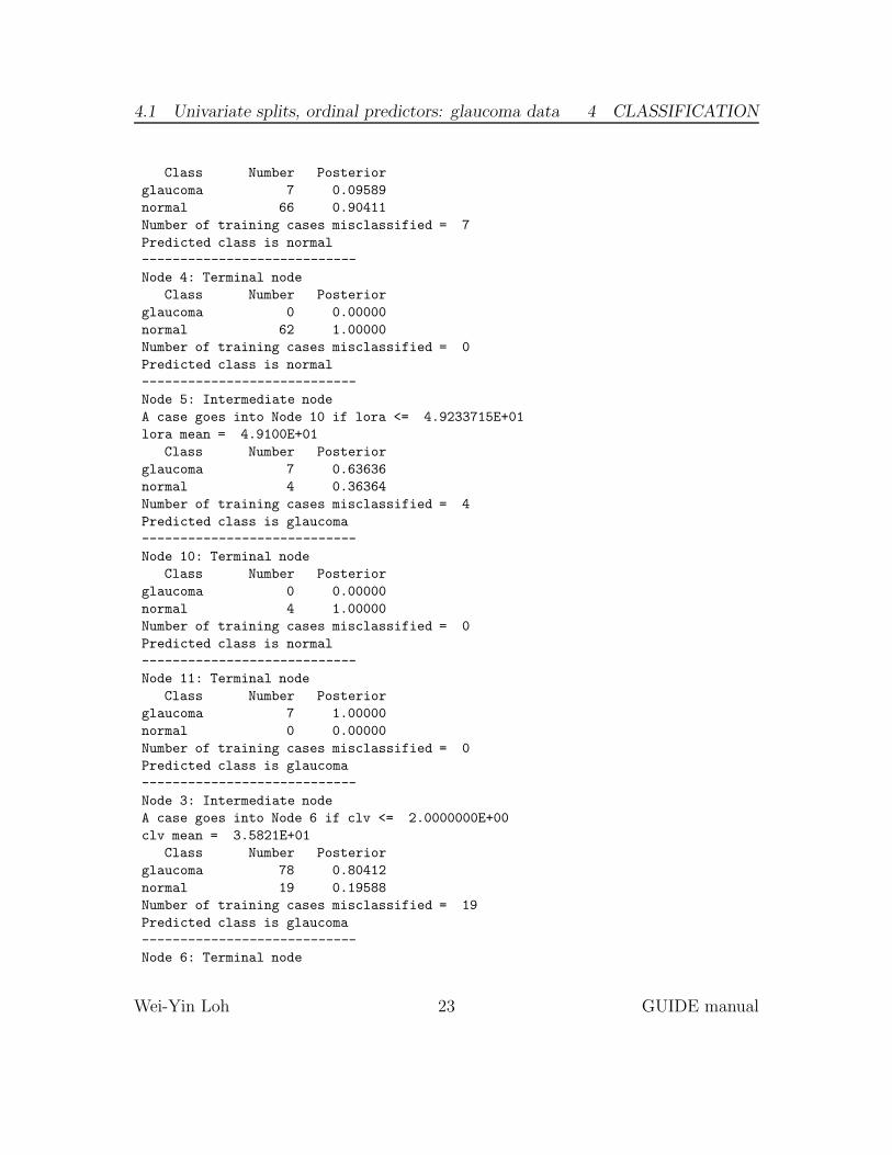
Node 4: Terminal node
Class Number Posterior
glaucoma 0 0.00000
normal 62 1.00000
Number of training cases misclassified = 0
Predicted class is normal
----------------------------
Node 5: Intermediate node
A case goes into Node 10 if lora <= 4.9233715E+01
lora mean = 4.9100E+01
Class Number Posterior
glaucoma 7 0.63636
normal 4 0.36364
Number of training cases misclassified = 4
Predicted class is glaucoma
----------------------------
Node 10: Terminal node
Class Number Posterior
glaucoma 0 0.00000
normal 4 1.00000
Number of training cases misclassified = 0
Predicted class is normal
----------------------------
Node 11: Terminal node
Class Number Posterior
glaucoma 7 1.00000
normal 0 0.00000
Number of training cases misclassified = 0
Predicted class is glaucoma
----------------------------
Node 3: Intermediate node
A case goes into Node 6 if clv <= 2.0000000E+00
clv mean = 3.5821E+01
Class Number Posterior
glaucoma 78 0.80412
normal 19 0.19588
Number of training cases misclassified = 19
Predicted class is glaucoma
----------------------------
Node 6: Terminal node
Wei-Yin Loh 23 GUIDE manual

4.1 Univariate splits, ordinal predictors: glaucoma data 4 CLASSIFICATION
Class Number Posterior
glaucoma 1 0.06667
normal 14 0.93333
Number of training cases misclassified = 1
Predicted class is normal
----------------------------
Node 7: Terminal node
Class Number Posterior
glaucoma 77 0.93902
normal 5 0.06098
Number of training cases misclassified = 5
Predicted class is glaucoma
----------------------------
Classification matrix for training sample:
Predicted True class
class glaucoma normal
glaucoma 84 5
normal 1 80
Total 85 85
Number of cases used for tree construction: 170
Number misclassified: 6
Resubstitution est. of mean misclassification cost: 0.3529E-01
Observed and fitted values are stored in glaucoma.fit
LaTeX code for tree is in glaucoma.tex
Figure 1 shows the classification tree drawn by LaTeX using the file glaucoma.tex.The last sentence in its caption gives the second best variable for splitting the rootnode. The top lines of the file glaucoma.fit are shown below. Their order corre-sponds to the order of the observations in the training sample file. The 1st column(labeled train) indicates whether the observation is used (“y”) or not used (“n”) tofit the model. Since we used the entire data set to fit the model here, all the entriesin the first column are y. The 2nd column gives the terminal node number that theobservation belongs to and the 3rd and 4th columns give its observed and predictedclasses. The last two columns give the number of glaucoma and normal observationsin the node where the observation belongs. They may be used to estimate the classprobabilities in the node.
train node observed predicted glaucoma normal
y 4 "normal" "normal" 0 62
y 4 "normal" "normal" 0 62
y 4 "normal" "normal" 0 62
y 4 "normal" "normal" 0 62
Wei-Yin Loh 24 GUIDE manual

4.1 Univariate splits, ordinal predictors: glaucoma data 4 CLASSIFICATION
lora≤56.40 1
clv≤∗8.40 2
062 4
normal
lora≤49.23 5
04 10
normal
11
glaucoma
70
clv≤2.00 3
114 6
normal
7
glaucoma
775
0 20 40 60 80
050
100
150
lora
clv
glaucomanormal
Figure 1: GUIDE v.27.9 0.50-SE classification tree for predicting Class using esti-mated priors and unit misclassification costs. At each split, an observation goes tothe left branch if and only if the condition is satisfied. The symbol ‘≤∗’ stands for‘≤ or missing’. Predicted classes (based on estimated misclassification cost) printedbelow terminal nodes; sample sizes for Class = glaucoma and normal, respectively,beside nodes. Second best split variable at root node is clv.
Wei-Yin Loh 25 GUIDE manual

4.2 Linear splits: glaucoma data 4 CLASSIFICATION
y 6 "normal" "normal" 1 14
4.2 Linear splits: glaucoma data
This section shows how to make GUIDE use linear splits on two variables at a time.
0. Read the warranty disclaimer
1. Create an input file for model fitting or importance scoring (recommended)
2. Convert data to other formats without creating input file
Input your choice: 1
Name of batch input file: lin.in
Input 1 for model fitting, 2 for importance or DIF scoring,
3 for data conversion ([1:3], <cr>=1):
Name of batch output file: lin.out
Input 1 for single tree, 2 for ensemble ([1:2], <cr>=1):
Input 1 for classification, 2 for regression, 3 for propensity score grouping
(propensity score grouping is an experimental option)
Input your choice ([1:3], <cr>=1):
Input 1 for default options, 2 otherwise ([1:2], <cr>=1):2
Choosing 2 enables more options.
Input 1 for simple, 2 for nearest-neighbor, 3 for kernel method
([1:3], <cr>=1):
Options 2 and 3 yield nearest-neighbor and kernel discriminant node models.
Input 0 for linear, interaction and univariate splits (in this order),
1 for univariate, linear and interaction splits (in this order),
2 to skip linear splits,
3 to skip linear and interaction splits:
Input your choice ([0:3], <cr>=1):0
Option 1 is the default.
Input 1 to prune by CV, 2 by test sample, 3 for no pruning ([1:3], <cr>=1):
Input name of data description file (max 100 characters);
enclose with matching quotes if it has spaces: glaucoma.dsc
Reading data description file ...
Training sample file: glaucoma.rdata
Missing value code: NA
Records in data file start on line 2
Warning: N variables changed to S
Dependent variable is Class
Reading data file ...
Number of records in data file: 170
Length of longest data entry: 8
Checking for missing values ...
Total number of cases: 170
Number of classes: 2
Wei-Yin Loh 26 GUIDE manual

4.2 Linear splits: glaucoma data 4 CLASSIFICATION
Re-checking data ...
Allocating missing value information
Assigning codes to categorical and missing values
Finished checking data
Creating missing value indicators
Rereading data
Class #Cases Proportion
glaucoma 85 0.50000000
normal 85 0.50000000
Total #cases w/ #missing
#cases miss. D ord. vals #X-var #N-var #F-var #S-var #B-var #C-var
170 0 17 0 0 0 66 0 0
No. cases used for training: 170
No. cases excluded due to 0 weight or missing D: 0
Finished reading data file
Default number of cross-validations: 10
Input 1 to accept the default, 2 to change it ([1:2], <cr>=1):
Best tree may be chosen based on mean or median CV estimate
Input 1 for mean-based, 2 for median-based ([1:2], <cr>=1):
Input number of SEs for pruning ([0.00:1000.00], <cr>=0.50):
Choose 1 for estimated priors, 2 for equal priors, 3 for priors from a file
Input 1, 2, or 3 ([1:3], <cr>=1):
Choose 1 for unit misclassification costs, 2 to input costs from a file
Input 1 or 2 ([1:2], <cr>=1):
Choose a split point selection method for numerical variables:
Choose 1 to use faster method based on sample quantiles
Choose 2 to use exhaustive search
Input 1 or 2 ([1:2], <cr>=2):
Default max number of split levels: 10
Input 1 to accept this value, 2 to change it ([1:2], <cr>=1):
Default minimum node sample size is 10
Input 1 to use the default value, 2 to change it ([1:2], <cr>=1):
Input 1 for LaTeX tree code, 2 to skip it ([1:2], <cr>=1):
Input file name to store LaTeX code (use .tex as suffix): lin.tex
Input 1 to include node numbers, 2 to omit them ([1:2], <cr>=1):
Choosing 2 will give a tree with no node labels.
Input 1 to number all nodes, 2 to number leaves only ([1:2], <cr>=1):
Input 1 to color terminal nodes, 2 otherwise ([1:2], <cr>=1):
Choose amount of detail in nodes of LaTeX tree diagram
Input 0 for #errors, 1 for class sizes, 2 for nothing ([0:2], <cr>=1):
Choose 2 if a large tree is expected.
You can store the variables and/or values used to split and fit in a file
Choose 1 to skip this step, 2 to store split variables and their values
Input your choice ([1:2], <cr>=1): 2
Choose 2 to output the info to another file for further processing.
Input file name: linvar.txt
Wei-Yin Loh 27 GUIDE manual
4.2 Linear splits: glaucoma data 4 CLASSIFICATION
Input 2 to save individual fitted values and node IDs, 1 otherwise ([1:2], <cr>=2):
Input name of file to store node ID and fitted value of each case: lin.fit
Input 2 to save terminal node IDs for importance scoring; 1 otherwise ([1:2], <cr>=1):
Input 2 to write R function for predicting new cases, 1 otherwise ([1:2], <cr>=1):2
Input file name: linpred.r
Input file is created!
Run GUIDE with the command: guide < lin.in
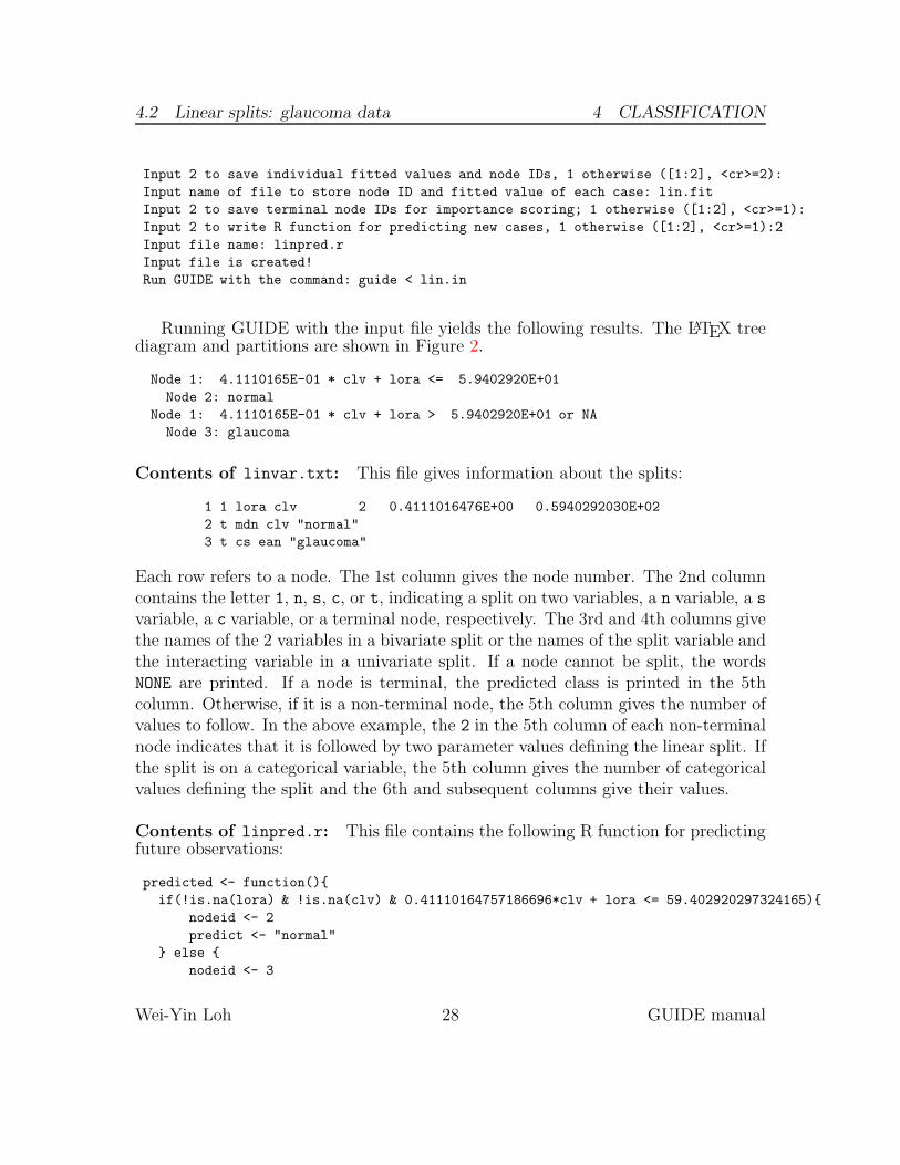
Running GUIDE with the input file yields the following results. The LATEX treediagram and partitions are shown in Figure 2.
Node 1: 4.1110165E-01 * clv + lora <= 5.9402920E+01
Node 2: normal
Node 1: 4.1110165E-01 * clv + lora > 5.9402920E+01 or NA
Node 3: glaucoma
Contents of linvar.txt: This file gives information about the splits:
1 1 lora clv 2 0.4111016476E+00 0.5940292030E+02
2 t mdn clv "normal"
3 t cs ean "glaucoma"
Each row refers to a node. The 1st column gives the node number. The 2nd columncontains the letter 1, n, s, c, or t, indicating a split on two variables, a n variable, a svariable, a c variable, or a terminal node, respectively. The 3rd and 4th columns givethe names of the 2 variables in a bivariate split or the names of the split variable andthe interacting variable in a univariate split. If a node cannot be split, the wordsNONE are printed. If a node is terminal, the predicted class is printed in the 5thcolumn. Otherwise, if it is a non-terminal node, the 5th column gives the number ofvalues to follow. In the above example, the 2 in the 5th column of each non-terminalnode indicates that it is followed by two parameter values defining the linear split. Ifthe split is on a categorical variable, the 5th column gives the number of categoricalvalues defining the split and the 6th and subsequent columns give their values.
Contents of linpred.r: This file contains the following R function for predictingfuture observations:
predicted <- function(){
if(!is.na(lora) & !is.na(clv) & 0.41110164757186696*clv + lora <= 59.402920297324165){
nodeid <- 2
predict <- "normal"
} else {
nodeid <- 3
Wei-Yin Loh 28 GUIDE manual

4.2 Linear splits: glaucoma data 4 CLASSIFICATION
loraclv 1
271 2
normal
3
glaucoma
8314
0 20 40 60 80
050
100
150
lora
clv glaucoma
normal
Figure 2: GUIDE v.27.9 0.50-SE classification tree for predicting Class using linearsplit priority, estimated priors and unit misclassification costs. At each split, anobservation goes to the left branch if and only if the condition is satisfied. Predictedclasses (based on estimated misclassification cost) printed below terminal nodes;sample sizes for Class = glaucoma and normal, respectively, beside nodes.
Wei-Yin Loh 29 GUIDE manual

4.3 Univariate splits, categorical predictors: peptide data 4 CLASSIFICATION
predict <- "glaucoma"
}
return(c(nodeid,predict))
}
4.3 Univariate splits, categorical predictors: peptide data
GUIDE can be used with categorical (i.e., nominal) predictor variables as well. Weshow this with a data set on peptide binding analyzed by Segal (1988) who usedCART. The data consist of observations on 310 peptides, 181 of which bind to aClass I MHC molecule and 129 do not. The data are in the file peptide.rdata.Column 1 contains the peptide ID and column 2 its binding status (bind). Theremaining 112 columns are predictor variables, all continuous except for the last 8which are categorical (named pos1–pos8), each taking 18–20 nominal values. Ourgoal here is to build a model to predict bind from these 8 categorical variables.
The GUIDE description is peptide.dsc. Note that the 3rd line of the file is“2”, indicating that the data begin on line 2 of peptide.rdata (the first line of thelatter contain the names of the variables). Note also that the continuous variablesare excluded from the model by designating each of them with an “x”.
4.3.1 Input file generation
We use all the default options to produce a GUIDE input file.
0. Read the warranty disclaimer
1. Create an input file for model fitting or importance scoring (recommended)
2. Convert data to other formats without creating input file
Input your choice: 1
Name of batch input file: peptide.in
Input 1 for model fitting, 2 for importance or DIF scoring,
3 for data conversion ([1:3], <cr>=1):
Name of batch output file: peptide.out
Input 1 for single tree, 2 for ensemble ([1:2], <cr>=1):
Input 1 for classification, 2 for regression, 3 for propensity score grouping
(propensity score grouping is an experimental option)
Input your choice ([1:3], <cr>=1):
Input 1 for default options, 2 otherwise ([1:2], <cr>=1):
Input name of data description file (max 100 characters);
enclose with matching quotes if it has spaces: peptide.dsc
Reading data description file ...
Training sample file: peptide.rdata
Missing value code: NA
Wei-Yin Loh 30 GUIDE manual

4.3 Univariate splits, categorical predictors: peptide data 4 CLASSIFICATION
Records in data file start on line 2
Dependent variable is bind
Reading data file ...
Number of records in data file: 310
Length of longest data entry: 6
Checking for missing values ...
Total number of cases: 310
Number of classes = 2
Col. no. Categorical variable #levels #missing values
107 pos1 18 0
108 pos2 20 0
109 pos3 20 0
110 pos4 20 0
111 pos5 20 0
112 pos6 20 0
113 pos7 19 0
114 pos8 20 0
Re-checking data ...
Assigning codes to categorical and missing values
Finished checking data
Rereading data
Class #Cases Proportion
0 129 0.41612903
1 181 0.58387097
Total #cases w/ #missing
#cases miss. D ord. vals #X-var #N-var #F-var #S-var #B-var #C-var
310 0 0 105 0 0 0 0 8
No. cases used for training: 310
Finished reading data file
Choose 1 for estimated priors, 2 for equal priors, 3 for priors from a file
Input 1, 2, or 3 ([1:3], <cr>=1):
Choose 1 for unit misclassification costs, 2 to input costs from a file
Input 1 or 2 ([1:2], <cr>=1):
Input 1 for LaTeX tree code, 2 to skip it ([1:2], <cr>=1):
Input file name to store LaTeX code (use .tex as suffix): peptide.tex
Input 2 to save individual fitted values and node IDs, 1 otherwise ([1:2], <cr>=2):
Input name of file to store node ID and fitted value of each case: peptide.fit
Input file is created!
Run GUIDE with the command: guide < peptide.in
4.3.2 Results
Results from the output file peptide.out follow.
Classification tree
Wei-Yin Loh 31 GUIDE manual

4.3 Univariate splits, categorical predictors: peptide data 4 CLASSIFICATION
Pruning by cross-validation
Data description file: peptide.dsc
Training sample file: peptide.rdata
Missing value code: NA
Records in data file start on line 2
Dependent variable is bind
Number of records in data file: 310
Length of longest entry in data file: 6
Number of classes: 2
Training sample class proportions of D variable bind:
Class #Cases Proportion
0 129 0.41612903
1 181 0.58387097
Summary information (without x variables)
d=dependent, b=split and fit cat variable using 0-1 dummies,
c=split-only categorical, n=split and fit numerical, f=fit-only numerical,
s=split-only numerical, w=weight
Column Name Minimum Maximum #Categories #Missing
2 bind d 2
107 pos1 c 18
108 pos2 c 20
109 pos3 c 20
110 pos4 c 20
111 pos5 c 20
112 pos6 c 20
113 pos7 c 19
114 pos8 c 20
Total #cases w/ #missing
#cases miss. D ord. vals #X-var #N-var #F-var #S-var #B-var #C-var
310 0 0 105 0 0 0 0 8
No. cases used for training: 310
Univariate split highest priority
Interaction and linear splits 2nd and 3rd priorities
Pruning by v-fold cross-validation, with v = 10
Selected tree is based on mean of CV estimates
Simple node models
Estimated priors
Unit misclassification costs
Split values for N and S variables based on exhaustive search
Max. number of split levels: 10
Min. node sample size: 2
Number of SE’s for pruned tree: 5.0000E-01
Wei-Yin Loh 32 GUIDE manual

4.3 Univariate splits, categorical predictors: peptide data 4 CLASSIFICATION
Size and CV mean cost and SE of subtrees:
Tree #Tnodes Mean Cost SE(Mean) BSE(Mean) Median Cost BSE(Median)
1 10 1.097E-01 1.775E-02 2.409E-02 9.677E-02 2.879E-02
2 8 1.097E-01 1.775E-02 2.409E-02 9.677E-02 2.879E-02
3 6 1.097E-01 1.775E-02 2.242E-02 9.677E-02 2.416E-02
4 5 1.097E-01 1.775E-02 2.206E-02 8.065E-02 2.231E-02
5 3 1.194E-01 1.841E-02 2.150E-02 1.129E-01 2.576E-02
6** 2 1.097E-01 1.775E-02 2.286E-02 8.065E-02 2.670E-02
7 1 4.161E-01 2.800E-02 3.207E-03 4.194E-01 1.019E-03
0-SE tree based on mean is marked with * and has 2 terminal nodes
0-SE tree based on median is marked with + and has 2 terminal nodes
Selected-SE tree based on mean using naive SE is marked with **
Selected-SE tree based on mean using bootstrap SE is marked with --
Selected-SE tree based on median and bootstrap SE is marked with ++
* tree, ** tree, + tree, and ++ tree all the same
Following tree is based on mean CV with naive SE estimate (**).
Structure of final tree. Each terminal node is marked with a T.
Node cost is node misclassification cost divided by number of training cases
Node Total Train Predicted Node Split Interacting
label cases cases class cost variables variable
1 310 310 1 4.161E-01 pos5
2T 169 169 1 5.917E-02 pos1
3T 141 141 0 1.560E-01 pos8
Number of terminal nodes of final tree: 2
Total number of nodes of final tree: 3
Second best split variable (based on curvature test) at root node is pos1
Classification tree:
Node 1: pos5 = "F", "M", "Y"
Node 2: 1
Node 1: pos5 /= "F", "M", "Y"
Node 3: 0
***************************************************************
Node 1: Intermediate node
A case goes into Node 2 if pos5 =
"F", "M", "Y"
pos5 mode = "Y"
Wei-Yin Loh 33 GUIDE manual

4.3 Univariate splits, categorical predictors: peptide data 4 CLASSIFICATION
Class Number Posterior
0 129 0.41613
1 181 0.58387
Number of training cases misclassified = 129
Predicted class is 1
----------------------------
Node 2: Terminal node
Class Number Posterior
0 10 0.05917
1 159 0.94083
Number of training cases misclassified = 10
Predicted class is 1
----------------------------
Node 3: Terminal node
Class Number Posterior
0 119 0.84397
1 22 0.15603
Number of training cases misclassified = 22
Predicted class is 0
----------------------------
Classification matrix for training sample:
Predicted True class
class 0 1
0 119 22
1 10 159
Total 129 181
Number of cases used for tree construction: 310
Number misclassified: 32
Resubstitution est. of mean misclassification cost: 0.1032
Observed and fitted values are stored in peptide.fit
LaTeX code for tree is in peptide.tex
The results indicate that the largest tree before pruning has 10 terminal nodes.The pruned tree (marked by “**”) has 2 terminal nodes. Its cross-validation estimateof misclassification cost (or error rate here) is 0.1097. Figure 3 shows the prunedtree. It splits on pos5, sending values F, M and Y to the left node. The second bestvariable to split the root node is pos1.
Wei-Yin Loh 34 GUIDE manual

4.4 Unbalanced classes and equal priors: hepatitis data 4 CLASSIFICATION
pos5
in S1 10.420.58
0.060.94 2
1169
3
0141
0.840.16
Figure 3: GUIDE v.27.9 0.50-SE classification tree for predicting bind using esti-mated priors and unit misclassification costs. At each split, an observation goes tothe left branch if and only if the condition is satisfied. Set S1 = {F, M, Y}. Predictedclasses and sample sizes printed below terminal nodes; class proportions for bind =0 and 1 beside nodes. Second best split variable at root node is pos1.
4.4 Unbalanced classes and equal priors: hepatitis data
If a data set has one dominant class, a classification tree may be null after pruning,as it may be hard to beat the classifier that predicts every observation to belong tothe dominant class. Nonetheless, it may be of interest to find out which variablesare more predictive and how they affect the dependent variable. One solution is touse the equal priors option. The resulting model should not be used for prediction.Instead, by comparing the class proportions in each terminal node against thoseat the root node, it can be used to identify the nodes where the dominant classproportion is much higher or much lower than average (i.e., at the root node).
We use a hepatitis data set to show this. The files are hepdsc.txt and hepdat.txt;see http://archive.ics.uci.edu/ml/datasets/Hepatitis. The data consist ofobservations from 155 individuals, of whom 32 are labeled “die’’ and 123 labeled“live’’. That is, 79% of the individuals are in the “live” class. The contents ofhepdsc.txt are:
hepdat.txt
"?"
1
1 CLASS d
2 AGE n
3 SEX c
4 STEROID c
5 ANTIVIRALS c
6 FATIGUE c
7 MALAISE c
8 ANOREXIA c
9 BIGLIVER c
Wei-Yin Loh 35 GUIDE manual
4.4 Unbalanced classes and equal priors: hepatitis data 4 CLASSIFICATION
ASCITES= yes 1
0.210.79
0.700.30 2
die20
3
live135
0.130.87
ASCITES= yes 1
0.210.79
0.700.30 2
die20
SPIDERS= no 3
0.050.95 6
live93
7
die42
0.310.69
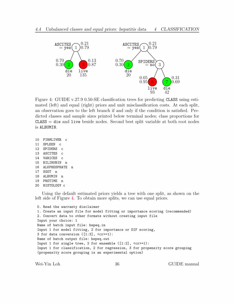
Figure 4: GUIDE v.27.9 0.50-SE classification trees for predicting CLASS using esti-mated (left) and equal (right) priors and unit misclassification costs. At each split,an observation goes to the left branch if and only if the condition is satisfied. Pre-dicted classes and sample sizes printed below terminal nodes; class proportions forCLASS = die and live beside nodes. Second best split variable at both root nodesis ALBUMIN.
10 FIRMLIVER c
11 SPLEEN c
12 SPIDERS c
13 ASCITES c
14 VARICES c
15 BILIRUBIN n
16 ALKPHOSPHATE n
17 SGOT n
18 ALBUMIN n
19 PROTIME n
20 HISTOLOGY c
Using the default estimated priors yields a tree with one split, as shown on theleft side of Figure 4. To obtain more splits, we can use equal priors.
0. Read the warranty disclaimer
1. Create an input file for model fitting or importance scoring (recommended)
2. Convert data to other formats without creating input file
Input your choice: 1
Name of batch input file: hepeq.in
Input 1 for model fitting, 2 for importance or DIF scoring,
3 for data conversion ([1:3], <cr>=1):
Name of batch output file: hepeq.out
Input 1 for single tree, 2 for ensemble ([1:2], <cr>=1):
Input 1 for classification, 2 for regression, 3 for propensity score grouping
(propensity score grouping is an experimental option)
Wei-Yin Loh 36 GUIDE manual

4.4 Unbalanced classes and equal priors: hepatitis data 4 CLASSIFICATION
Input your choice ([1:3], <cr>=1):
Input 1 for default options, 2 otherwise ([1:2], <cr>=1): 2
Option 2 is needed for equal or specified priors.
Input 1 for simple, 2 for nearest-neighbor, 3 for kernel method ([1:3], <cr>=1):
Input 0 for linear, interaction and univariate splits (in this order),
1 for univariate, linear and interaction splits (in this order),
2 to skip linear splits,
3 to skip linear and interaction splits:
Input your choice ([0:3], <cr>=1):
Input 1 to prune by CV, 2 by test sample, 3 for no pruning ([1:3], <cr>=1):
Input name of data description file (max 100 characters);
enclose with matching quotes if it has spaces: hepdsc.txt
Reading data description file ...
Training sample file: hepdat.txt
Missing value code: ?
Records in data file start on line 1
Warning: N variables changed to S
Dependent variable is CLASS
Reading data file ...
Number of records in data file: 155
Length of longest data entry: 6
Checking for missing values ...
Total number of cases: 155
Missing values found among categorical variables
Separate categories will be created for missing categorical variables
Number of classes: 2
Col. no. Categorical variable #levels #missing values
3 SEX 2 0
4 STEROID 2 1
5 ANTIVIRALS 2 0
6 FATIGUE 2 1
7 MALAISE 2 1
8 ANOREXIA 2 1
9 BIGLIVER 2 10
10 FIRMLIVER 2 11
11 SPLEEN 2 5
12 SPIDERS 2 5
13 ASCITES 2 5
14 VARICES 2 5
20 HISTOLOGY 2 0
Re-checking data ...
Allocating missing value information
Assigning codes to categorical and missing values
Data checks complete
Creating missing value indicators
Wei-Yin Loh 37 GUIDE manual

4.4 Unbalanced classes and equal priors: hepatitis data 4 CLASSIFICATION
Rereading data
Class #Cases Proportion
die 32 0.20645161
live 123 0.79354839
Total #cases w/ #missing
#cases miss. D ord. vals #X-var #N-var #F-var #S-var #B-var #C-var
155 0 72 0 0 0 6 0 13
No. cases used for training: 155
No. cases excluded due to 0 weight or missing D: 0
Finished reading data file
Default number of cross-validations: 10
Input 1 to accept the default, 2 to change it ([1:2], <cr>=1):
Best tree may be chosen based on mean or median CV estimate
Input 1 for mean-based, 2 for median-based ([1:2], <cr>=1):
Input number of SEs for pruning ([0.00:1000.00], <cr>=0.50):
Choose 1 for estimated priors, 2 for equal priors, 3 for priors from a file
Input 1, 2, or 3 ([1:3], <cr>=1):2
Option 2 is for equal priors.
Choose 1 for unit misclassification costs, 2 to input costs from a file
Input 1 or 2 ([1:2], <cr>=1):
Choose a split point selection method for numerical variables:
Choose 1 to use faster method based on sample quantiles
Choose 2 to use exhaustive search
Input 1 or 2 ([1:2], <cr>=2):
Default max. number of split levels: 10
Input 1 to accept this value, 2 to change it ([1:2], <cr>=1):
Default minimum node sample size is 2
Input 1 to use the default value, 2 to change it ([1:2], <cr>=1):
Input 1 for LaTeX tree code, 2 to skip it ([1:2], <cr>=1):
Input file name to store LaTeX code (use .tex as suffix): hepeq.tex
Input 1 to include node numbers, 2 to omit them ([1:2], <cr>=1):
Input 1 to number all nodes, 2 to number leaves only ([1:2], <cr>=1):
Input 1 to color terminal nodes, 2 otherwise ([1:2], <cr>=1):
Choose amount of detail in nodes of LaTeX tree diagram
Input 0 for #errors, 1 for class sizes, 2 for nothing ([0:2], <cr>=1):
You can store the variables and/or values used to split and fit in a file
Choose 1 to skip this step, 2 to store split and fit variables,
3 to store split variables and their values
Input your choice ([1:3], <cr>=1):3
Input file name: hepvar.txt
Contents of this file are shown below.
Input 2 to save individual fitted values and node IDs, 1 otherwise ([1:2], <cr>=2):
Input name of file to store node ID and fitted value of each case: hepeq.fit
Input 2 to write R function for predicting new cases, 1 otherwise ([1:2], <cr>=1):
Input file is created!
Run GUIDE with the command: guide < hepeq.in
Wei-Yin Loh 38 GUIDE manual
4.5 Unequal misclassification costs: hepatitis data 4 CLASSIFICATION
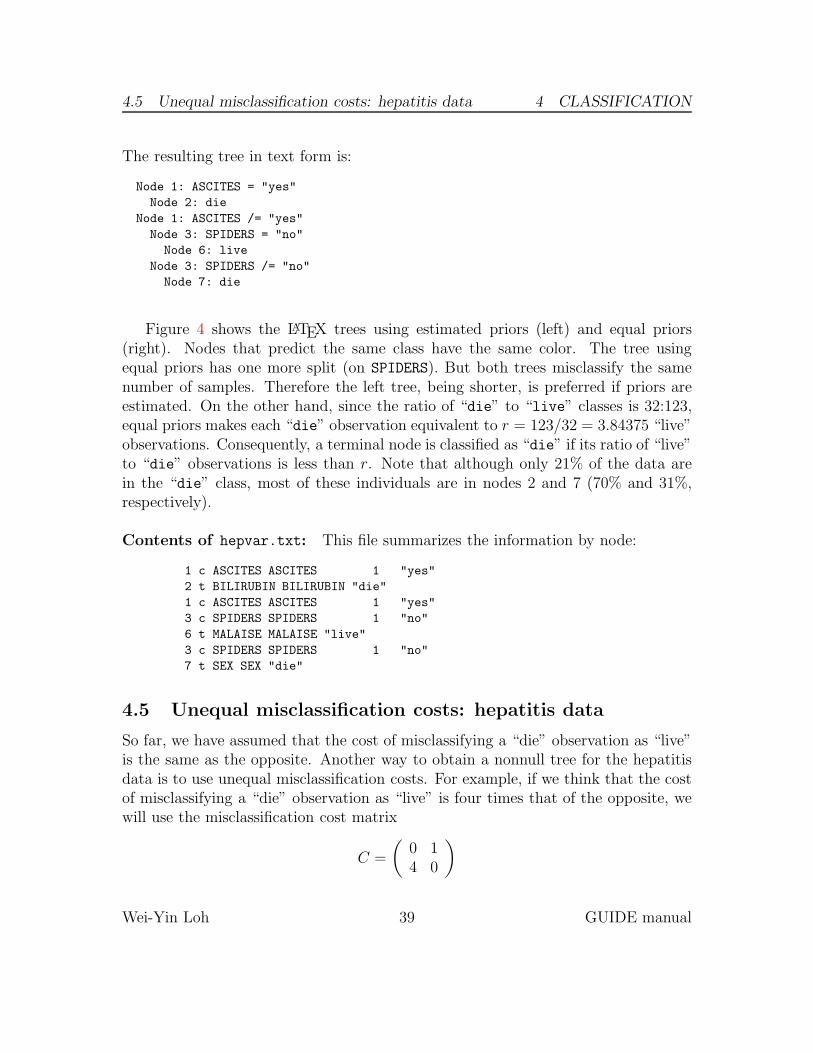
The resulting tree in text form is:
Node 1: ASCITES = "yes"
Node 2: die
Node 1: ASCITES /= "yes"
Node 3: SPIDERS = "no"
Node 6: live
Node 3: SPIDERS /= "no"
Node 7: die
Figure 4 shows the LATEX trees using estimated priors (left) and equal priors(right). Nodes that predict the same class have the same color. The tree usingequal priors has one more split (on SPIDERS). But both trees misclassify the samenumber of samples. Therefore the left tree, being shorter, is preferred if priors areestimated. On the other hand, since the ratio of “die” to “live” classes is 32:123,equal priors makes each “die” observation equivalent to r = 123/32 = 3.84375 “live”observations. Consequently, a terminal node is classified as “die” if its ratio of “live”to “die” observations is less than r. Note that although only 21% of the data arein the “die” class, most of these individuals are in nodes 2 and 7 (70% and 31%,respectively).
Contents of hepvar.txt: This file summarizes the information by node:
1 c ASCITES ASCITES 1 "yes"
2 t BILIRUBIN BILIRUBIN "die"
1 c ASCITES ASCITES 1 "yes"
3 c SPIDERS SPIDERS 1 "no"
6 t MALAISE MALAISE "live"
3 c SPIDERS SPIDERS 1 "no"
7 t SEX SEX "die"
4.5 Unequal misclassification costs: hepatitis data
So far, we have assumed that the cost of misclassifying a “die” observation as “live”is the same as the opposite. Another way to obtain a nonnull tree for the hepatitisdata is to use unequal misclassification costs. For example, if we think that the costof misclassifying a “die” observation as “live” is four times that of the opposite, wewill use the misclassification cost matrix
C =
(
0 14 0
)
Wei-Yin Loh 39 GUIDE manual

4.6 More than 2 classes: dermatology 4 CLASSIFICATION
where C(i, j) denotes the cost of classifying an observation as class i given that itbelongs to class j. Note that GUIDE sorts the class values in alphabetical order, sothat “die” is treated as class 1 and “live” as class 2 here. This matrix is saved in thetext file cost.txt which has these two lines:
0 1
4 0
The following lines in the input file generation step shows where this file is used:
Choose 1 for estimated priors, 2 for equal priors, 3 to input the priors from a file
Input 1, 2, or 3 ([1:3], <cr>=1):
Choose 1 for unit misclassification costs, 2 to input costs from a file
Input 1 or 2 ([1:2], <cr>=1): 2
Input the name of a file containing the cost matrix C(i|j),
where C(i|j) is the cost of classifying class j as class i
The rows of the matrix must be in alphabetical order of the class names
Input name of file: cost.txt
The resulting tree is the same as that for equal priors in Figure 4.
4.6 More than 2 classes: dermatology with ordinal predic-tors
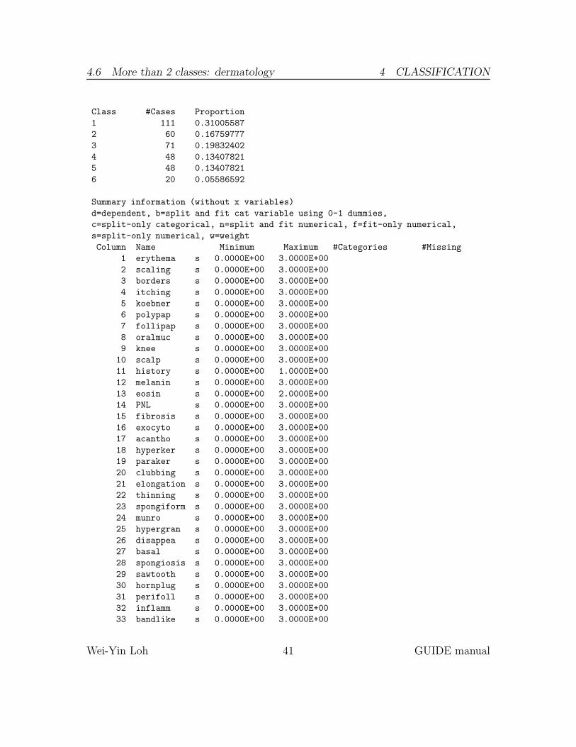
The data, taken from UCI (Ilter and Guvenir, 1998), give the diagnosis (6 classes)and clinical and laboratory measurements of 34 ordinal predictor variables for 358patients. The description and data files are derm.dsc and derm.dat, respectively.
4.6.1 Default option
The default option gives the following results.
Classification tree
Pruning by cross-validation
Data description file: derm.dsc
Training sample file: derm.dat
Missing value code: ?
Records in data file start on line 1
Warning: N variables changed to S
Dependent variable is class
Number of records in data file: 358
Length of longest data entry: 2
Number of classes: 6
Class proportions of dependent variable class:
Wei-Yin Loh 40 GUIDE manual
4.6 More than 2 classes: dermatology 4 CLASSIFICATION
Class #Cases Proportion
1 111 0.31005587
2 60 0.16759777
3 71 0.19832402
4 48 0.13407821
5 48 0.13407821
6 20 0.05586592
Summary information (without x variables)
d=dependent, b=split and fit cat variable using 0-1 dummies,
c=split-only categorical, n=split and fit numerical, f=fit-only numerical,
s=split-only numerical, w=weight
Column Name Minimum Maximum #Categories #Missing
1 erythema s 0.0000E+00 3.0000E+00
2 scaling s 0.0000E+00 3.0000E+00
3 borders s 0.0000E+00 3.0000E+00
4 itching s 0.0000E+00 3.0000E+00
5 koebner s 0.0000E+00 3.0000E+00
6 polypap s 0.0000E+00 3.0000E+00
7 follipap s 0.0000E+00 3.0000E+00
8 oralmuc s 0.0000E+00 3.0000E+00
9 knee s 0.0000E+00 3.0000E+00
10 scalp s 0.0000E+00 3.0000E+00
11 history s 0.0000E+00 1.0000E+00
12 melanin s 0.0000E+00 3.0000E+00
13 eosin s 0.0000E+00 2.0000E+00
14 PNL s 0.0000E+00 3.0000E+00
15 fibrosis s 0.0000E+00 3.0000E+00
16 exocyto s 0.0000E+00 3.0000E+00
17 acantho s 0.0000E+00 3.0000E+00
18 hyperker s 0.0000E+00 3.0000E+00
19 paraker s 0.0000E+00 3.0000E+00
20 clubbing s 0.0000E+00 3.0000E+00
21 elongation s 0.0000E+00 3.0000E+00
22 thinning s 0.0000E+00 3.0000E+00
23 spongiform s 0.0000E+00 3.0000E+00
24 munro s 0.0000E+00 3.0000E+00
25 hypergran s 0.0000E+00 3.0000E+00
26 disappea s 0.0000E+00 3.0000E+00
27 basal s 0.0000E+00 3.0000E+00
28 spongiosis s 0.0000E+00 3.0000E+00
29 sawtooth s 0.0000E+00 3.0000E+00
30 hornplug s 0.0000E+00 3.0000E+00
31 perifoll s 0.0000E+00 3.0000E+00
32 inflamm s 0.0000E+00 3.0000E+00
33 bandlike s 0.0000E+00 3.0000E+00
Wei-Yin Loh 41 GUIDE manual

4.6 More than 2 classes: dermatology 4 CLASSIFICATION
34 age s 0.0000E+00 7.5000E+01
35 class d 6
Total #cases w/ #missing
#cases miss. D ord. vals #X-var #N-var #F-var #S-var #B-var #C-var
358 0 0 0 0 0 34 0 0
No. cases used for training: 358
Univariate split highest priority
Interaction and linear splits 2nd and 3rd priorities
Pruning by v-fold cross-validation, with v = 10
Selected tree is based on mean of CV estimates
Simple node models
Estimated priors
Unit misclassification costs
Split values for N and S variables based on exhaustive search
Max. number of split levels: 10
Min. node sample size: 2
Number of SE’s for pruned tree: 5.0000E-01
Size and CV mean cost and SE of subtrees:
Tree #Tnodes Mean Cost SE(Mean) BSE(Mean) Median Cost BSE(Median)
1 12 3.631E-02 9.887E-03 9.649E-03 2.778E-02 7.256E-03
2 10 3.631E-02 9.887E-03 9.649E-03 2.778E-02 7.256E-03
3** 9 3.631E-02 9.887E-03 9.649E-03 2.778E-02 7.256E-03
4++ 8 5.307E-02 1.185E-02 1.713E-02 2.778E-02 1.611E-02
5 7 5.866E-02 1.242E-02 1.720E-02 4.167E-02 2.080E-02
6 5 1.788E-01 2.025E-02 2.914E-02 1.690E-01 2.707E-02
7 2 4.804E-01 2.641E-02 2.058E-02 4.722E-01 2.831E-02
8 1 6.899E-01 2.444E-02 2.184E-02 6.806E-01 2.412E-02
0-SE tree based on mean is marked with *
0-SE tree based on median is marked with +
Selected-SE tree based on mean using naive SE is marked with **
Selected-SE tree based on mean using bootstrap SE is marked with --
Selected-SE tree based on median and bootstrap SE is marked with ++
** tree same as -- tree
+ tree same as ++ tree
* tree same as ** tree
* tree same as -- tree
Following tree is based on mean CV with naive SE estimate (**).
Structure of final tree. Each terminal node is marked with a T.
Node cost is node misclassification cost divided by number of training cases
Wei-Yin Loh 42 GUIDE manual
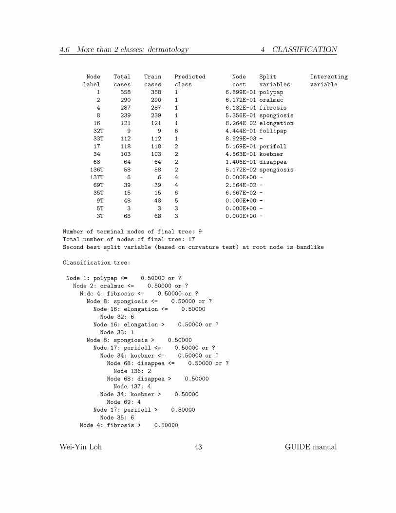
4.6 More than 2 classes: dermatology 4 CLASSIFICATION
Node Total Train Predicted Node Split Interacting
label cases cases class cost variables variable
1 358 358 1 6.899E-01 polypap
2 290 290 1 6.172E-01 oralmuc
4 287 287 1 6.132E-01 fibrosis
8 239 239 1 5.356E-01 spongiosis
16 121 121 1 8.264E-02 elongation
32T 9 9 6 4.444E-01 follipap
33T 112 112 1 8.929E-03 -
17 118 118 2 5.169E-01 perifoll
34 103 103 2 4.563E-01 koebner
68 64 64 2 1.406E-01 disappea
136T 58 58 2 5.172E-02 spongiosis
137T 6 6 4 0.000E+00 -
69T 39 39 4 2.564E-02 -
35T 15 15 6 6.667E-02 -
9T 48 48 5 0.000E+00 -
5T 3 3 3 0.000E+00 -
3T 68 68 3 0.000E+00 -
Number of terminal nodes of final tree: 9
Total number of nodes of final tree: 17
Second best split variable (based on curvature test) at root node is bandlike
Classification tree:
Node 1: polypap <= 0.50000 or ?
Node 2: oralmuc <= 0.50000 or ?
Node 4: fibrosis <= 0.50000 or ?
Node 8: spongiosis <= 0.50000 or ?
Node 16: elongation <= 0.50000
Node 32: 6
Node 16: elongation > 0.50000 or ?
Node 33: 1
Node 8: spongiosis > 0.50000
Node 17: perifoll <= 0.50000 or ?
Node 34: koebner <= 0.50000 or ?
Node 68: disappea <= 0.50000 or ?
Node 136: 2
Node 68: disappea > 0.50000
Node 137: 4
Node 34: koebner > 0.50000
Node 69: 4
Node 17: perifoll > 0.50000
Node 35: 6
Node 4: fibrosis > 0.50000
Wei-Yin Loh 43 GUIDE manual
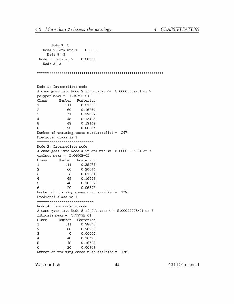
4.6 More than 2 classes: dermatology 4 CLASSIFICATION
Node 9: 5
Node 2: oralmuc > 0.50000
Node 5: 3
Node 1: polypap > 0.50000
Node 3: 3
***************************************************************
Node 1: Intermediate node
A case goes into Node 2 if polypap <= 5.0000000E-01 or ?
polypap mean = 4.4972E-01
Class Number Posterior
1 111 0.31006
2 60 0.16760
3 71 0.19832
4 48 0.13408
5 48 0.13408
6 20 0.05587
Number of training cases misclassified = 247
Predicted class is 1
----------------------------
Node 2: Intermediate node
A case goes into Node 4 if oralmuc <= 5.0000000E-01 or ?
oralmuc mean = 2.0690E-02
Class Number Posterior
1 111 0.38276
2 60 0.20690
3 3 0.01034
4 48 0.16552
5 48 0.16552
6 20 0.06897
Number of training cases misclassified = 179
Predicted class is 1
----------------------------
Node 4: Intermediate node
A case goes into Node 8 if fibrosis <= 5.0000000E-01 or ?
fibrosis mean = 3.7979E-01
Class Number Posterior
1 111 0.38676
2 60 0.20906
3 0 0.00000
4 48 0.16725
5 48 0.16725
6 20 0.06969
Number of training cases misclassified = 176
Wei-Yin Loh 44 GUIDE manual

4.6 More than 2 classes: dermatology 4 CLASSIFICATION
Predicted class is 1
----------------------------
Node 8: Intermediate node
A case goes into Node 16 if spongiosis <= 5.0000000E-01 or ?
spongiosis mean = 1.0544E+00
Class Number Posterior
1 111 0.46444
2 60 0.25105
3 0 0.00000
4 48 0.20084
5 0 0.00000
6 20 0.08368
Number of training cases misclassified = 128
Predicted class is 1
----------------------------
Node 16: Intermediate node
A case goes into Node 32 if elongation <= 5.0000000E-01
elongation mean = 2.0909E+00
Class Number Posterior
1 111 0.91736
2 3 0.02479
3 0 0.00000
4 1 0.00826
5 0 0.00000
6 6 0.04959
Number of training cases misclassified = 10
Predicted class is 1
----------------------------
Node 32: Terminal node
Class Number Posterior
1 0 0.00000
2 3 0.33333
3 0 0.00000
4 1 0.11111
5 0 0.00000
6 5 0.55556
Number of training cases misclassified = 4
Predicted class is 6
----------------------------
Node 33: Terminal node
Class Number Posterior
1 111 0.99107
2 0 0.00000
3 0 0.00000
4 0 0.00000
5 0 0.00000
Wei-Yin Loh 45 GUIDE manual

4.6 More than 2 classes: dermatology 4 CLASSIFICATION
6 1 0.00893
Number of training cases misclassified = 1
Predicted class is 1
----------------------------
Node 17: Intermediate node
A case goes into Node 34 if perifoll <= 5.0000000E-01 or ?
perifoll mean = 2.6271E-01
Class Number Posterior
1 0 0.00000
2 57 0.48305
3 0 0.00000
4 47 0.39831
5 0 0.00000
6 14 0.11864
Number of training cases misclassified = 61
Predicted class is 2
----------------------------
Node 34: Intermediate node
A case goes into Node 68 if koebner <= 5.0000000E-01 or ?
koebner mean = 5.4369E-01
Class Number Posterior
1 0 0.00000
2 56 0.54369
3 0 0.00000
4 47 0.45631
5 0 0.00000
6 0 0.00000
Number of training cases misclassified = 47
Predicted class is 2
----------------------------
Node 68: Intermediate node
A case goes into Node 136 if disappea <= 5.0000000E-01 or ?
disappea mean = 9.3750E-02
Class Number Posterior
1 0 0.00000
2 55 0.85938
3 0 0.00000
4 9 0.14063
5 0 0.00000
6 0 0.00000
Number of training cases misclassified = 9
Predicted class is 2
----------------------------
Node 136: Terminal node
Class Number Posterior
1 0 0.00000
Wei-Yin Loh 46 GUIDE manual
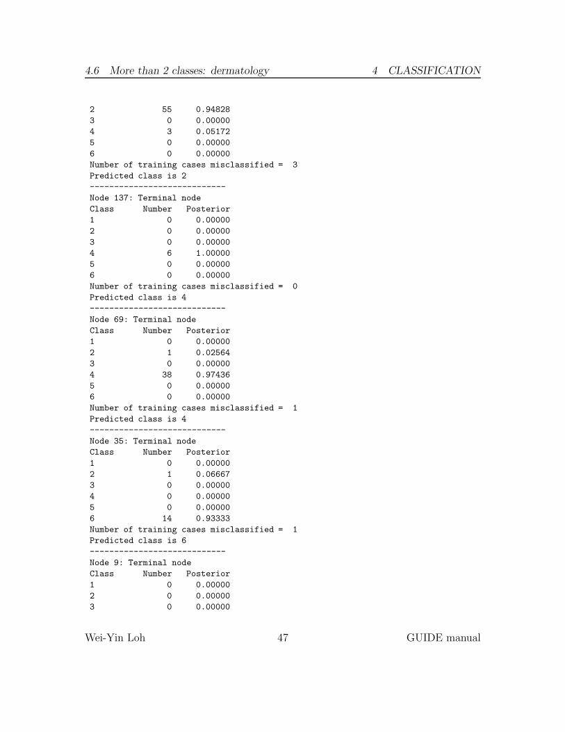
4.6 More than 2 classes: dermatology 4 CLASSIFICATION
2 55 0.94828
3 0 0.00000
4 3 0.05172
5 0 0.00000
6 0 0.00000
Number of training cases misclassified = 3
Predicted class is 2
----------------------------
Node 137: Terminal node
Class Number Posterior
1 0 0.00000
2 0 0.00000
3 0 0.00000
4 6 1.00000
5 0 0.00000
6 0 0.00000
Number of training cases misclassified = 0
Predicted class is 4
----------------------------
Node 69: Terminal node
Class Number Posterior
1 0 0.00000
2 1 0.02564
3 0 0.00000
4 38 0.97436
5 0 0.00000
6 0 0.00000
Number of training cases misclassified = 1
Predicted class is 4
----------------------------
Node 35: Terminal node
Class Number Posterior
1 0 0.00000
2 1 0.06667
3 0 0.00000
4 0 0.00000
5 0 0.00000
6 14 0.93333
Number of training cases misclassified = 1
Predicted class is 6
----------------------------
Node 9: Terminal node
Class Number Posterior
1 0 0.00000
2 0 0.00000
3 0 0.00000
Wei-Yin Loh 47 GUIDE manual

4.6 More than 2 classes: dermatology 4 CLASSIFICATION
4 0 0.00000
5 48 1.00000
6 0 0.00000
Number of training cases misclassified = 0
Predicted class is 5
----------------------------
Node 5: Terminal node
Class Number Posterior
1 0 0.00000
2 0 0.00000
3 3 1.00000
4 0 0.00000
5 0 0.00000
6 0 0.00000
Number of training cases misclassified = 0
Predicted class is 3
----------------------------
Node 3: Terminal node
Class Number Posterior
1 0 0.00000
2 0 0.00000
3 68 1.00000
4 0 0.00000
5 0 0.00000
6 0 0.00000
Number of training cases misclassified = 0
Predicted class is 3
----------------------------
Classification matrix for training sample:
Predicted True class
class 1 2 3 4 5 6
1 111 0 0 0 0 1
2 0 55 0 3 0 0
3 0 0 71 0 0 0
4 0 1 0 44 0 0
5 0 0 0 0 48 0
6 0 4 0 1 0 19
Total 111 60 71 48 48 20
Number of cases used for tree construction: 358
Number misclassified: 10
Resubstitution est. of mean misclassification cost: 0.2793E-01
Wei-Yin Loh 48 GUIDE manual

4.6 More than 2 classes: dermatology 4 CLASSIFICATION
Observed and fitted values are stored in derm.fit
LaTeX code for tree is in derm.tex
The tree is shown in Figure 5; it misclassifies 10 observations.
4.6.2 Nearest-neighbor option
One way to obtain a smaller tree is to fit a classification model to the data in eachnode and use it to classify the individual observations there. GUIDE has two meansto achieve this: nearest-neighbor and kernel discrimination. For nearest-neighbor, anobservation in a node is classified to the plurality class among observations within itsneighborhood. The neighborhood is defined to be the whole node if the split variableis categorical. The input file for this option is obtained as follows.
Input file creation
0. Read the warranty disclaimer
1. Create an input file for model fitting or importance scoring (recommended)
2. Convert data to other formats without creating input file
Input your choice: 1
Name of batch input file: nn.in
Input 1 for model fitting, 2 for importance or DIF scoring,
3 for data conversion ([1:3], <cr>=1):
Name of batch output file: nn.out
Input 1 for single tree, 2 for ensemble ([1:2], <cr>=1):
Input 1 for classification, 2 for regression, 3 for propensity score grouping
(propensity score grouping is an experimental option)
Input your choice ([1:3], <cr>=1):
Input 1 for default options, 2 otherwise ([1:2], <cr>=1): 2
Input 1 for simple, 2 for nearest-neighbor, 3 for kernel method ([1:3], <cr>=1): 2
Choose nearest-neighbor option here.
Input 1 for univariate, 2 for bivariate preference ([1:2], <cr>=1):
Default is univariate kernels.
Input 1 for interaction tests, 2 to skip them ([1:2], <cr>=1):
Input 1 to prune by CV, 2 by test sample, 3 for no pruning ([1:3], <cr>=1):
Input name of data description file (max 100 characters);
enclose with matching quotes if it has spaces: derm.dsc
Reading data description file ...
Training sample file: derm.dat
Missing value code: ?
Records in data file start on line 1
Warning: N variables changed to S
Wei-Yin Loh 49 GUIDE manual

4.6 More than 2 classes: dermatology 4 CLASSIFICATION
polypap≤∗.5000 1
358
oralmuc≤∗.5000 2
fibrosis≤∗.5000 4
spongiosis≤∗.5000 8
elongation≤ .5000 16
4 32
69
33
1112
1
perifoll≤∗.5000 17
koebner≤∗.5000 34
disappea≤∗.5000 68
3 136
258
137
46
0
69
439
1
35
615
1
9
548
0
5
33
0
3
368
0
Figure 5: GUIDE v.27.9 0.50-SE classification tree for predicting class using es-timated priors and unit misclassification costs. At each split, an observation goesto the left branch if and only if the condition is satisfied. The symbol ‘≤∗’ standsfor ‘≤ or missing’. Predicted classes and sample sizes printed below terminal nodes;#misclassified beside nodes. Second best split variable at root node is bandlike.
Wei-Yin Loh 50 GUIDE manual
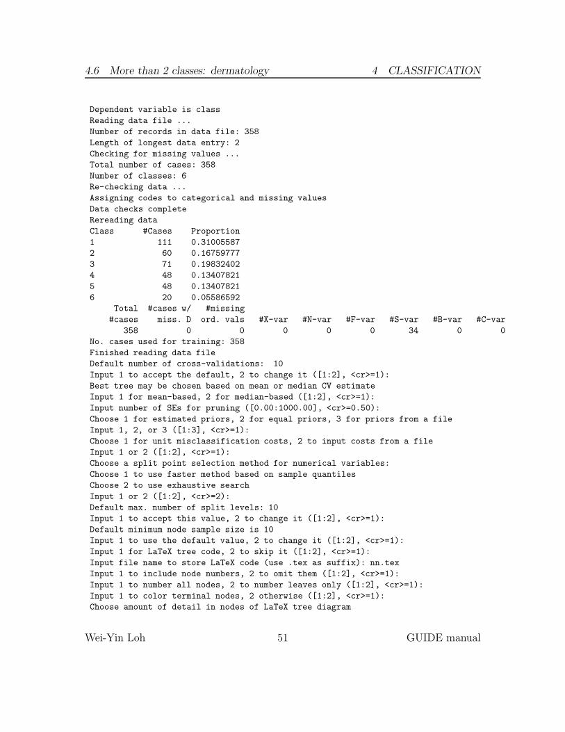
4.6 More than 2 classes: dermatology 4 CLASSIFICATION
Dependent variable is class
Reading data file ...
Number of records in data file: 358
Length of longest data entry: 2
Checking for missing values ...
Total number of cases: 358
Number of classes: 6
Re-checking data ...
Assigning codes to categorical and missing values
Data checks complete
Rereading data
Class #Cases Proportion
1 111 0.31005587
2 60 0.16759777
3 71 0.19832402
4 48 0.13407821
5 48 0.13407821
6 20 0.05586592
Total #cases w/ #missing
#cases miss. D ord. vals #X-var #N-var #F-var #S-var #B-var #C-var
358 0 0 0 0 0 34 0 0
No. cases used for training: 358
Finished reading data file
Default number of cross-validations: 10
Input 1 to accept the default, 2 to change it ([1:2], <cr>=1):
Best tree may be chosen based on mean or median CV estimate
Input 1 for mean-based, 2 for median-based ([1:2], <cr>=1):
Input number of SEs for pruning ([0.00:1000.00], <cr>=0.50):
Choose 1 for estimated priors, 2 for equal priors, 3 for priors from a file
Input 1, 2, or 3 ([1:3], <cr>=1):
Choose 1 for unit misclassification costs, 2 to input costs from a file
Input 1 or 2 ([1:2], <cr>=1):
Choose a split point selection method for numerical variables:
Choose 1 to use faster method based on sample quantiles
Choose 2 to use exhaustive search
Input 1 or 2 ([1:2], <cr>=2):
Default max. number of split levels: 10
Input 1 to accept this value, 2 to change it ([1:2], <cr>=1):
Default minimum node sample size is 10
Input 1 to use the default value, 2 to change it ([1:2], <cr>=1):
Input 1 for LaTeX tree code, 2 to skip it ([1:2], <cr>=1):
Input file name to store LaTeX code (use .tex as suffix): nn.tex
Input 1 to include node numbers, 2 to omit them ([1:2], <cr>=1):
Input 1 to number all nodes, 2 to number leaves only ([1:2], <cr>=1):
Input 1 to color terminal nodes, 2 otherwise ([1:2], <cr>=1):
Choose amount of detail in nodes of LaTeX tree diagram
Wei-Yin Loh 51 GUIDE manual
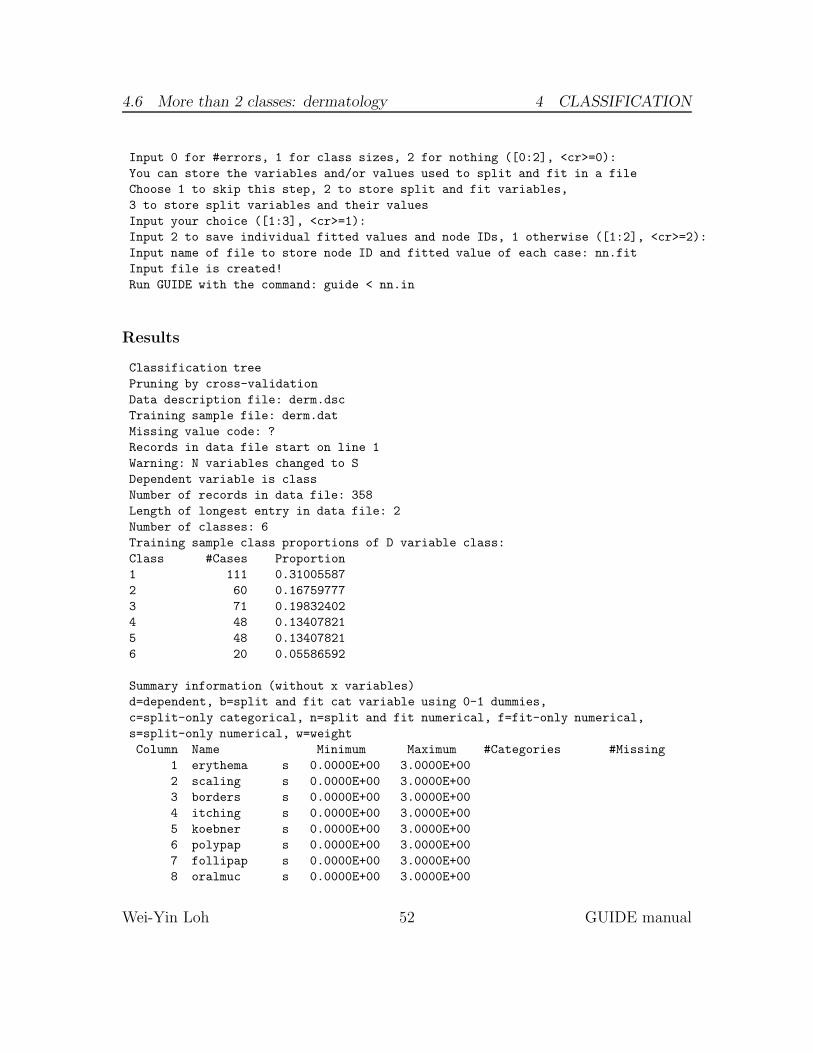
4.6 More than 2 classes: dermatology 4 CLASSIFICATION
Input 0 for #errors, 1 for class sizes, 2 for nothing ([0:2], <cr>=0):
You can store the variables and/or values used to split and fit in a file
Choose 1 to skip this step, 2 to store split and fit variables,
3 to store split variables and their values
Input your choice ([1:3], <cr>=1):
Input 2 to save individual fitted values and node IDs, 1 otherwise ([1:2], <cr>=2):
Input name of file to store node ID and fitted value of each case: nn.fit
Input file is created!
Run GUIDE with the command: guide < nn.in
Results
Classification tree
Pruning by cross-validation
Data description file: derm.dsc
Training sample file: derm.dat
Missing value code: ?
Records in data file start on line 1
Warning: N variables changed to S
Dependent variable is class
Number of records in data file: 358
Length of longest entry in data file: 2
Number of classes: 6
Training sample class proportions of D variable class:
Class #Cases Proportion
1 111 0.31005587
2 60 0.16759777
3 71 0.19832402
4 48 0.13407821
5 48 0.13407821
6 20 0.05586592
Summary information (without x variables)
d=dependent, b=split and fit cat variable using 0-1 dummies,
c=split-only categorical, n=split and fit numerical, f=fit-only numerical,
s=split-only numerical, w=weight
Column Name Minimum Maximum #Categories #Missing
1 erythema s 0.0000E+00 3.0000E+00
2 scaling s 0.0000E+00 3.0000E+00
3 borders s 0.0000E+00 3.0000E+00
4 itching s 0.0000E+00 3.0000E+00
5 koebner s 0.0000E+00 3.0000E+00
6 polypap s 0.0000E+00 3.0000E+00
7 follipap s 0.0000E+00 3.0000E+00
8 oralmuc s 0.0000E+00 3.0000E+00
Wei-Yin Loh 52 GUIDE manual
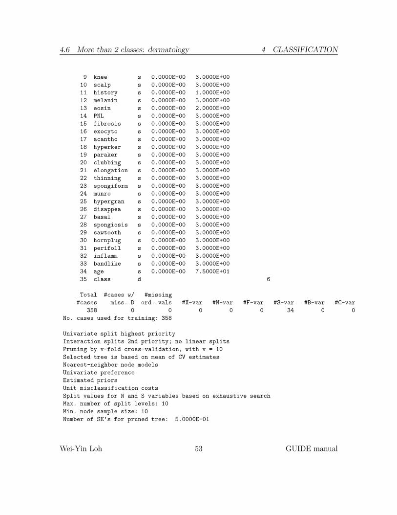
4.6 More than 2 classes: dermatology 4 CLASSIFICATION
9 knee s 0.0000E+00 3.0000E+00
10 scalp s 0.0000E+00 3.0000E+00
11 history s 0.0000E+00 1.0000E+00
12 melanin s 0.0000E+00 3.0000E+00
13 eosin s 0.0000E+00 2.0000E+00
14 PNL s 0.0000E+00 3.0000E+00
15 fibrosis s 0.0000E+00 3.0000E+00
16 exocyto s 0.0000E+00 3.0000E+00
17 acantho s 0.0000E+00 3.0000E+00
18 hyperker s 0.0000E+00 3.0000E+00
19 paraker s 0.0000E+00 3.0000E+00
20 clubbing s 0.0000E+00 3.0000E+00
21 elongation s 0.0000E+00 3.0000E+00
22 thinning s 0.0000E+00 3.0000E+00
23 spongiform s 0.0000E+00 3.0000E+00
24 munro s 0.0000E+00 3.0000E+00
25 hypergran s 0.0000E+00 3.0000E+00
26 disappea s 0.0000E+00 3.0000E+00
27 basal s 0.0000E+00 3.0000E+00
28 spongiosis s 0.0000E+00 3.0000E+00
29 sawtooth s 0.0000E+00 3.0000E+00
30 hornplug s 0.0000E+00 3.0000E+00
31 perifoll s 0.0000E+00 3.0000E+00
32 inflamm s 0.0000E+00 3.0000E+00
33 bandlike s 0.0000E+00 3.0000E+00
34 age s 0.0000E+00 7.5000E+01
35 class d 6
Total #cases w/ #missing
#cases miss. D ord. vals #X-var #N-var #F-var #S-var #B-var #C-var
358 0 0 0 0 0 34 0 0
No. cases used for training: 358
Univariate split highest priority
Interaction splits 2nd priority; no linear splits
Pruning by v-fold cross-validation, with v = 10
Selected tree is based on mean of CV estimates
Nearest-neighbor node models
Univariate preference
Estimated priors
Unit misclassification costs
Split values for N and S variables based on exhaustive search
Max. number of split levels: 10
Min. node sample size: 10
Number of SE’s for pruned tree: 5.0000E-01
Wei-Yin Loh 53 GUIDE manual
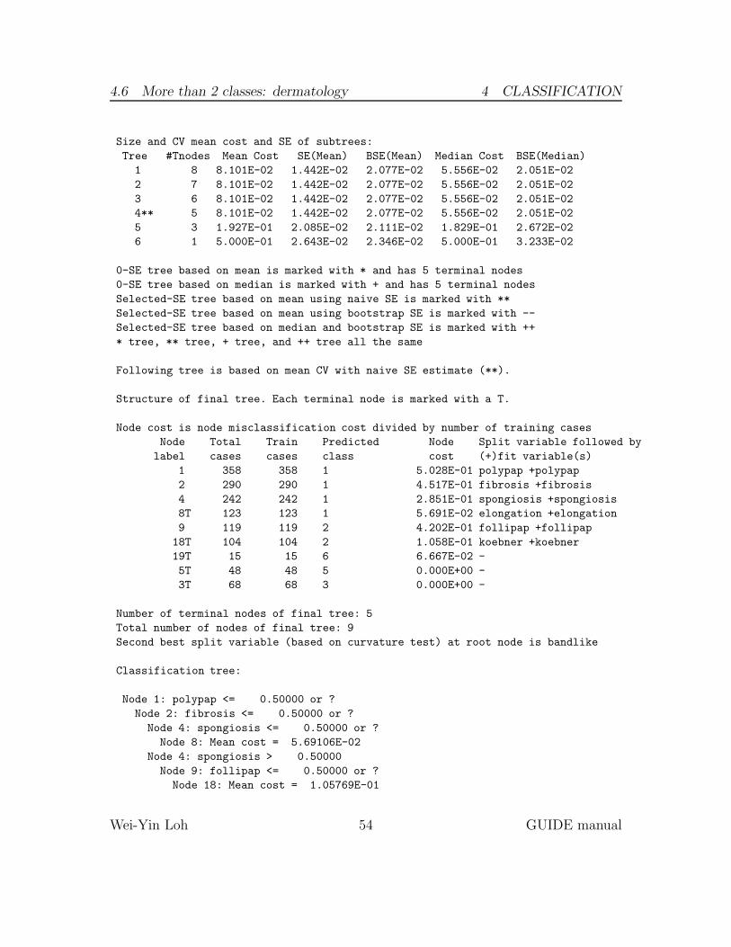
4.6 More than 2 classes: dermatology 4 CLASSIFICATION
Size and CV mean cost and SE of subtrees:
Tree #Tnodes Mean Cost SE(Mean) BSE(Mean) Median Cost BSE(Median)
1 8 8.101E-02 1.442E-02 2.077E-02 5.556E-02 2.051E-02
2 7 8.101E-02 1.442E-02 2.077E-02 5.556E-02 2.051E-02
3 6 8.101E-02 1.442E-02 2.077E-02 5.556E-02 2.051E-02
4** 5 8.101E-02 1.442E-02 2.077E-02 5.556E-02 2.051E-02
5 3 1.927E-01 2.085E-02 2.111E-02 1.829E-01 2.672E-02
6 1 5.000E-01 2.643E-02 2.346E-02 5.000E-01 3.233E-02
0-SE tree based on mean is marked with * and has 5 terminal nodes
0-SE tree based on median is marked with + and has 5 terminal nodes
Selected-SE tree based on mean using naive SE is marked with **
Selected-SE tree based on mean using bootstrap SE is marked with --
Selected-SE tree based on median and bootstrap SE is marked with ++
* tree, ** tree, + tree, and ++ tree all the same
Following tree is based on mean CV with naive SE estimate (**).
Structure of final tree. Each terminal node is marked with a T.
Node cost is node misclassification cost divided by number of training cases
Node Total Train Predicted Node Split variable followed by
label cases cases class cost (+)fit variable(s)
1 358 358 1 5.028E-01 polypap +polypap
2 290 290 1 4.517E-01 fibrosis +fibrosis
4 242 242 1 2.851E-01 spongiosis +spongiosis
8T 123 123 1 5.691E-02 elongation +elongation
9 119 119 2 4.202E-01 follipap +follipap
18T 104 104 2 1.058E-01 koebner +koebner
19T 15 15 6 6.667E-02 -
5T 48 48 5 0.000E+00 -
3T 68 68 3 0.000E+00 -
Number of terminal nodes of final tree: 5
Total number of nodes of final tree: 9
Second best split variable (based on curvature test) at root node is bandlike
Classification tree:
Node 1: polypap <= 0.50000 or ?
Node 2: fibrosis <= 0.50000 or ?
Node 4: spongiosis <= 0.50000 or ?
Node 8: Mean cost = 5.69106E-02
Node 4: spongiosis > 0.50000
Node 9: follipap <= 0.50000 or ?
Node 18: Mean cost = 1.05769E-01
Wei-Yin Loh 54 GUIDE manual
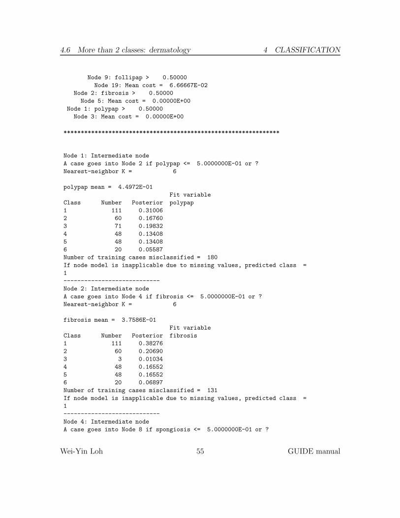
4.6 More than 2 classes: dermatology 4 CLASSIFICATION
Node 9: follipap > 0.50000
Node 19: Mean cost = 6.66667E-02
Node 2: fibrosis > 0.50000
Node 5: Mean cost = 0.00000E+00
Node 1: polypap > 0.50000
Node 3: Mean cost = 0.00000E+00
***************************************************************
Node 1: Intermediate node
A case goes into Node 2 if polypap <= 5.0000000E-01 or ?
Nearest-neighbor K = 6
polypap mean = 4.4972E-01
Fit variable
Class Number Posterior polypap
1 111 0.31006
2 60 0.16760
3 71 0.19832
4 48 0.13408
5 48 0.13408
6 20 0.05587
Number of training cases misclassified = 180
If node model is inapplicable due to missing values, predicted class =
1
----------------------------
Node 2: Intermediate node
A case goes into Node 4 if fibrosis <= 5.0000000E-01 or ?
Nearest-neighbor K = 6
fibrosis mean = 3.7586E-01
Fit variable
Class Number Posterior fibrosis
1 111 0.38276
2 60 0.20690
3 3 0.01034
4 48 0.16552
5 48 0.16552
6 20 0.06897
Number of training cases misclassified = 131
If node model is inapplicable due to missing values, predicted class =
1
----------------------------
Node 4: Intermediate node
A case goes into Node 8 if spongiosis <= 5.0000000E-01 or ?
Wei-Yin Loh 55 GUIDE manual

4.6 More than 2 classes: dermatology 4 CLASSIFICATION
Nearest-neighbor K = 6
spongiosis mean = 1.0537E+00
Fit variable
Class Number Posterior spongiosis
1 111 0.45868
2 60 0.24793
3 3 0.01240
4 48 0.19835
5 0 0.00000
6 20 0.08264
Number of training cases misclassified = 69
If node model is inapplicable due to missing values, predicted class =
1
----------------------------
Node 8: Terminal node
Nearest-neighbor K = 5
elongation mean = 2.0569E+00
Fit variable
Class Number Posterior elongation
1 111 0.90244
2 3 0.02439
3 2 0.01626
4 1 0.00813
5 0 0.00000
6 6 0.04878
----------------------------
Node 9: Intermediate node
A case goes into Node 18 if follipap <= 5.0000000E-01 or ?
Nearest-neighbor K = 5
follipap mean = 2.5210E-01
Fit variable
Class Number Posterior follipap
1 0 0.00000
2 57 0.47899
3 1 0.00840
4 47 0.39496
5 0 0.00000
6 14 0.11765
Number of training cases misclassified = 50
If node model is inapplicable due to missing values, predicted class =
2
----------------------------
Node 18: Terminal node
Nearest-neighbor K = 5
Wei-Yin Loh 56 GUIDE manual
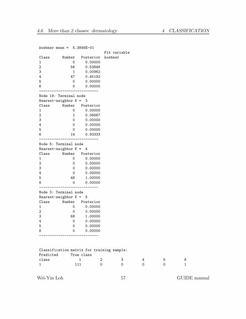
4.6 More than 2 classes: dermatology 4 CLASSIFICATION
koebner mean = 5.3846E-01
Fit variable
Class Number Posterior koebner
1 0 0.00000
2 56 0.53846
3 1 0.00962
4 47 0.45192
5 0 0.00000
6 0 0.00000
----------------------------
Node 19: Terminal node
Nearest-neighbor K = 3
Class Number Posterior
1 0 0.00000
2 1 0.06667
3 0 0.00000
4 0 0.00000
5 0 0.00000
6 14 0.93333
----------------------------
Node 5: Terminal node
Nearest-neighbor K = 4
Class Number Posterior
1 0 0.00000
2 0 0.00000
3 0 0.00000
4 0 0.00000
5 48 1.00000
6 0 0.00000
----------------------------
Node 3: Terminal node
Nearest-neighbor K = 5
Class Number Posterior
1 0 0.00000
2 0 0.00000
3 68 1.00000
4 0 0.00000
5 0 0.00000
6 0 0.00000
----------------------------
Classification matrix for training sample:
Predicted True class
class 1 2 3 4 5 6
1 111 0 0 0 0 1
Wei-Yin Loh 57 GUIDE manual
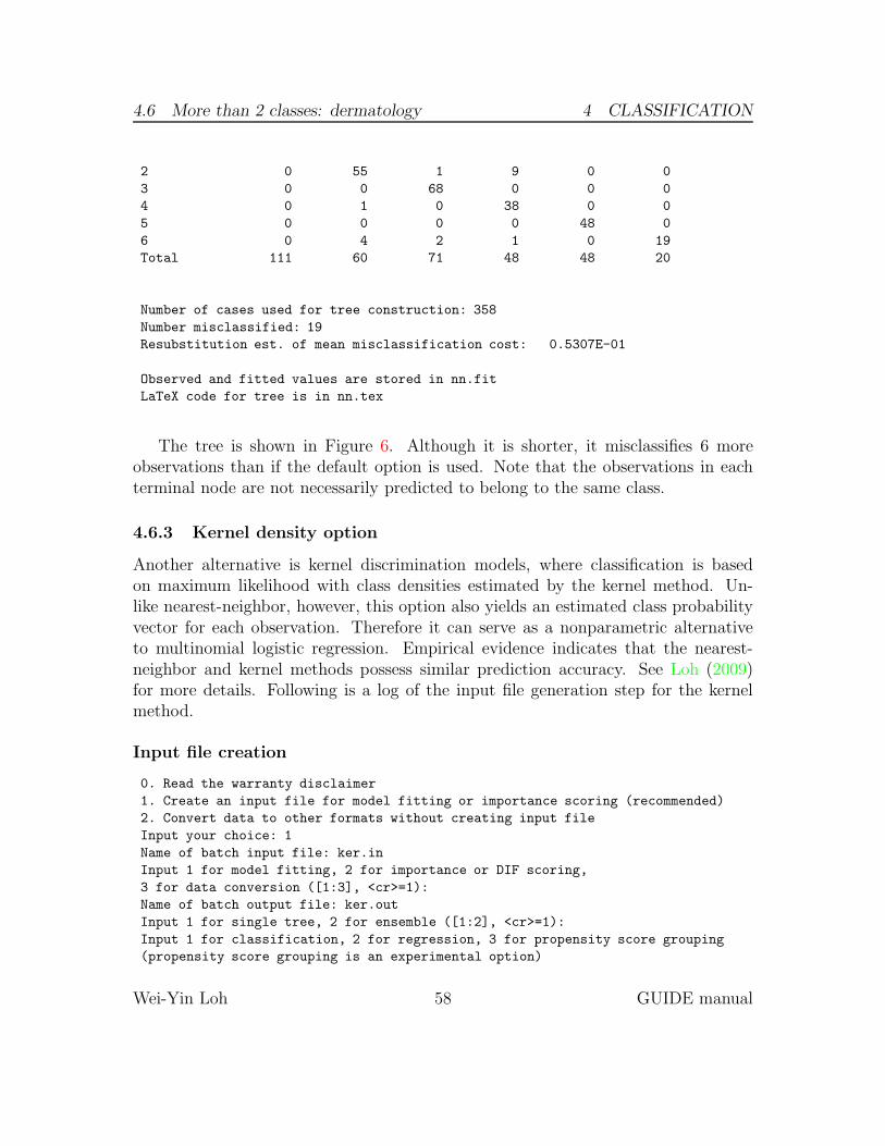
4.6 More than 2 classes: dermatology 4 CLASSIFICATION
2 0 55 1 9 0 0
3 0 0 68 0 0 0
4 0 1 0 38 0 0
5 0 0 0 0 48 0
6 0 4 2 1 0 19
Total 111 60 71 48 48 20
Number of cases used for tree construction: 358
Number misclassified: 19
Resubstitution est. of mean misclassification cost: 0.5307E-01
Observed and fitted values are stored in nn.fit
LaTeX code for tree is in nn.tex
The tree is shown in Figure 6. Although it is shorter, it misclassifies 6 moreobservations than if the default option is used. Note that the observations in eachterminal node are not necessarily predicted to belong to the same class.
4.6.3 Kernel density option
Another alternative is kernel discrimination models, where classification is basedon maximum likelihood with class densities estimated by the kernel method. Un-like nearest-neighbor, however, this option also yields an estimated class probabilityvector for each observation. Therefore it can serve as a nonparametric alternativeto multinomial logistic regression. Empirical evidence indicates that the nearest-neighbor and kernel methods possess similar prediction accuracy. See Loh (2009)for more details. Following is a log of the input file generation step for the kernelmethod.
Input file creation
0. Read the warranty disclaimer
1. Create an input file for model fitting or importance scoring (recommended)
2. Convert data to other formats without creating input file
Input your choice: 1
Name of batch input file: ker.in
Input 1 for model fitting, 2 for importance or DIF scoring,
3 for data conversion ([1:3], <cr>=1):
Name of batch output file: ker.out
Input 1 for single tree, 2 for ensemble ([1:2], <cr>=1):
Input 1 for classification, 2 for regression, 3 for propensity score grouping
(propensity score grouping is an experimental option)
Wei-Yin Loh 58 GUIDE manual

4.6 More than 2 classes: dermatology 4 CLASSIFICATION
polypap≤∗.5000 1
358
fibrosis≤∗.5000 2
spongiosis≤∗.5000 4
7 8
1123
follipap≤∗.5000 9
11 18
2104
19
615
1
5
548
0
3
368
0
Figure 6: GUIDE v.27.9 0.50-SE classification tree for predicting class using uni-variate nearest-neighbor node models, estimated priors and unit misclassificationcosts. At each split, an observation goes to the left branch if and only if the condi-tion is satisfied. The symbol ‘≤∗’ stands for ‘≤ or missing’. Predicted classes andsample sizes printed below terminal nodes; #misclassified beside nodes. Second bestsplit variable at root node is bandlike.
Wei-Yin Loh 59 GUIDE manual
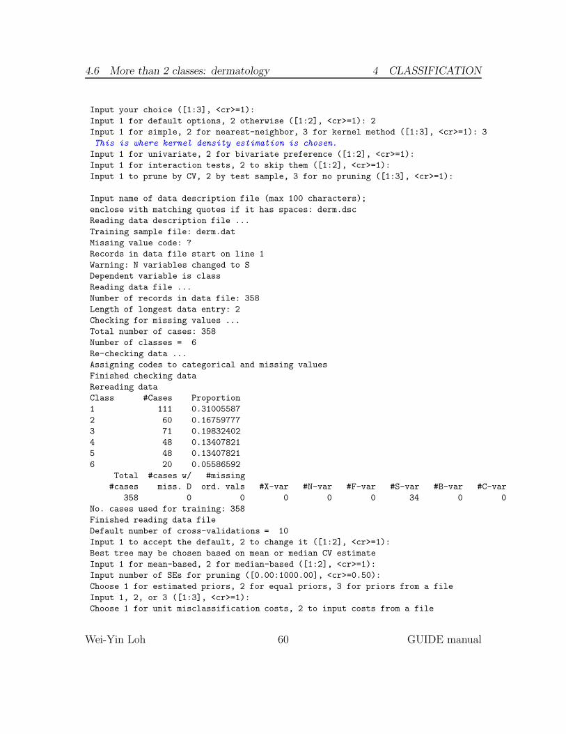
4.6 More than 2 classes: dermatology 4 CLASSIFICATION
Input your choice ([1:3], <cr>=1):
Input 1 for default options, 2 otherwise ([1:2], <cr>=1): 2
Input 1 for simple, 2 for nearest-neighbor, 3 for kernel method ([1:3], <cr>=1): 3
This is where kernel density estimation is chosen.
Input 1 for univariate, 2 for bivariate preference ([1:2], <cr>=1):
Input 1 for interaction tests, 2 to skip them ([1:2], <cr>=1):
Input 1 to prune by CV, 2 by test sample, 3 for no pruning ([1:3], <cr>=1):
Input name of data description file (max 100 characters);
enclose with matching quotes if it has spaces: derm.dsc
Reading data description file ...
Training sample file: derm.dat
Missing value code: ?
Records in data file start on line 1
Warning: N variables changed to S
Dependent variable is class
Reading data file ...
Number of records in data file: 358
Length of longest data entry: 2
Checking for missing values ...
Total number of cases: 358
Number of classes = 6
Re-checking data ...
Assigning codes to categorical and missing values
Finished checking data
Rereading data
Class #Cases Proportion
1 111 0.31005587
2 60 0.16759777
3 71 0.19832402
4 48 0.13407821
5 48 0.13407821
6 20 0.05586592
Total #cases w/ #missing
#cases miss. D ord. vals #X-var #N-var #F-var #S-var #B-var #C-var
358 0 0 0 0 0 34 0 0
No. cases used for training: 358
Finished reading data file
Default number of cross-validations = 10
Input 1 to accept the default, 2 to change it ([1:2], <cr>=1):
Best tree may be chosen based on mean or median CV estimate
Input 1 for mean-based, 2 for median-based ([1:2], <cr>=1):
Input number of SEs for pruning ([0.00:1000.00], <cr>=0.50):
Choose 1 for estimated priors, 2 for equal priors, 3 for priors from a file
Input 1, 2, or 3 ([1:3], <cr>=1):
Choose 1 for unit misclassification costs, 2 to input costs from a file
Wei-Yin Loh 60 GUIDE manual
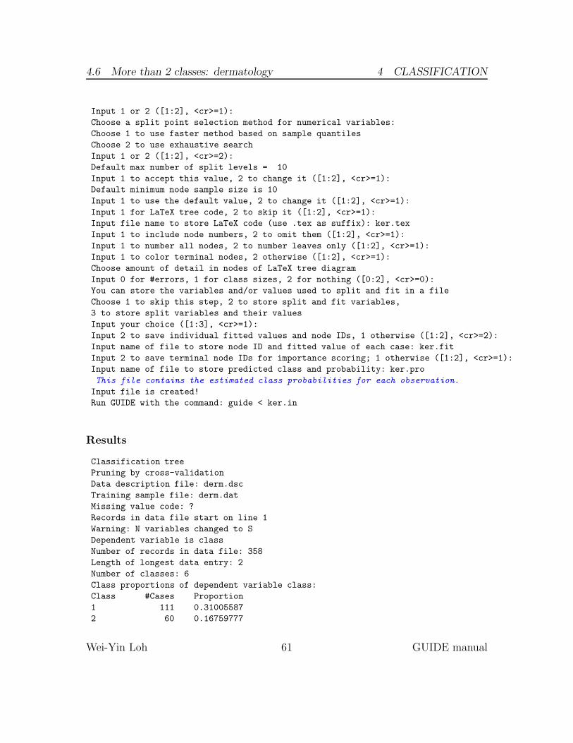
4.6 More than 2 classes: dermatology 4 CLASSIFICATION
Input 1 or 2 ([1:2], <cr>=1):
Choose a split point selection method for numerical variables:
Choose 1 to use faster method based on sample quantiles
Choose 2 to use exhaustive search
Input 1 or 2 ([1:2], <cr>=2):
Default max number of split levels = 10
Input 1 to accept this value, 2 to change it ([1:2], <cr>=1):
Default minimum node sample size is 10
Input 1 to use the default value, 2 to change it ([1:2], <cr>=1):
Input 1 for LaTeX tree code, 2 to skip it ([1:2], <cr>=1):
Input file name to store LaTeX code (use .tex as suffix): ker.tex
Input 1 to include node numbers, 2 to omit them ([1:2], <cr>=1):
Input 1 to number all nodes, 2 to number leaves only ([1:2], <cr>=1):
Input 1 to color terminal nodes, 2 otherwise ([1:2], <cr>=1):
Choose amount of detail in nodes of LaTeX tree diagram
Input 0 for #errors, 1 for class sizes, 2 for nothing ([0:2], <cr>=0):
You can store the variables and/or values used to split and fit in a file
Choose 1 to skip this step, 2 to store split and fit variables,
3 to store split variables and their values
Input your choice ([1:3], <cr>=1):
Input 2 to save individual fitted values and node IDs, 1 otherwise ([1:2], <cr>=2):
Input name of file to store node ID and fitted value of each case: ker.fit
Input 2 to save terminal node IDs for importance scoring; 1 otherwise ([1:2], <cr>=1):
Input name of file to store predicted class and probability: ker.pro
This file contains the estimated class probabilities for each observation.
Input file is created!
Run GUIDE with the command: guide < ker.in
Results
Classification tree
Pruning by cross-validation
Data description file: derm.dsc
Training sample file: derm.dat
Missing value code: ?
Records in data file start on line 1
Warning: N variables changed to S
Dependent variable is class
Number of records in data file: 358
Length of longest data entry: 2
Number of classes: 6
Class proportions of dependent variable class:
Class #Cases Proportion
1 111 0.31005587
2 60 0.16759777
Wei-Yin Loh 61 GUIDE manual
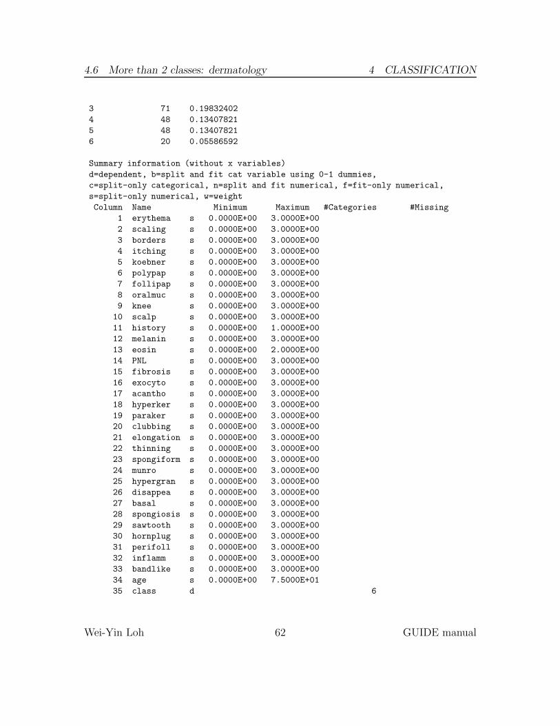
4.6 More than 2 classes: dermatology 4 CLASSIFICATION
3 71 0.19832402
4 48 0.13407821
5 48 0.13407821
6 20 0.05586592
Summary information (without x variables)
d=dependent, b=split and fit cat variable using 0-1 dummies,
c=split-only categorical, n=split and fit numerical, f=fit-only numerical,
s=split-only numerical, w=weight
Column Name Minimum Maximum #Categories #Missing
1 erythema s 0.0000E+00 3.0000E+00
2 scaling s 0.0000E+00 3.0000E+00
3 borders s 0.0000E+00 3.0000E+00
4 itching s 0.0000E+00 3.0000E+00
5 koebner s 0.0000E+00 3.0000E+00
6 polypap s 0.0000E+00 3.0000E+00
7 follipap s 0.0000E+00 3.0000E+00
8 oralmuc s 0.0000E+00 3.0000E+00
9 knee s 0.0000E+00 3.0000E+00
10 scalp s 0.0000E+00 3.0000E+00
11 history s 0.0000E+00 1.0000E+00
12 melanin s 0.0000E+00 3.0000E+00
13 eosin s 0.0000E+00 2.0000E+00
14 PNL s 0.0000E+00 3.0000E+00
15 fibrosis s 0.0000E+00 3.0000E+00
16 exocyto s 0.0000E+00 3.0000E+00
17 acantho s 0.0000E+00 3.0000E+00
18 hyperker s 0.0000E+00 3.0000E+00
19 paraker s 0.0000E+00 3.0000E+00
20 clubbing s 0.0000E+00 3.0000E+00
21 elongation s 0.0000E+00 3.0000E+00
22 thinning s 0.0000E+00 3.0000E+00
23 spongiform s 0.0000E+00 3.0000E+00
24 munro s 0.0000E+00 3.0000E+00
25 hypergran s 0.0000E+00 3.0000E+00
26 disappea s 0.0000E+00 3.0000E+00
27 basal s 0.0000E+00 3.0000E+00
28 spongiosis s 0.0000E+00 3.0000E+00
29 sawtooth s 0.0000E+00 3.0000E+00
30 hornplug s 0.0000E+00 3.0000E+00
31 perifoll s 0.0000E+00 3.0000E+00
32 inflamm s 0.0000E+00 3.0000E+00
33 bandlike s 0.0000E+00 3.0000E+00
34 age s 0.0000E+00 7.5000E+01
35 class d 6
Wei-Yin Loh 62 GUIDE manual

4.6 More than 2 classes: dermatology 4 CLASSIFICATION
Total #cases w/ #missing
#cases miss. D ord. vals #X-var #N-var #F-var #S-var #B-var #C-var
358 0 0 0 0 0 34 0 0
No. cases used for training: 358
Univariate split highest priority
Interaction splits 2nd priority; no linear splits
Pruning by v-fold cross-validation, with v = 10
Selected tree is based on mean of CV estimates
Kernel density node models
Univariate preference
Estimated priors
Unit misclassification costs
Split values for N and S variables based on exhaustive search
Max. number of split levels: 10
Min. node sample size: 10
Number of SE’s for pruned tree: 5.0000E-01
Size and CV mean cost and SE of subtrees:
Tree #Tnodes Mean Cost SE(Mean) BSE(Mean) Median Cost BSE(Median)
1 8 8.380E-02 1.464E-02 2.073E-02 6.944E-02 2.149E-02
2 7 8.380E-02 1.464E-02 2.073E-02 6.944E-02 2.149E-02
3 6 8.380E-02 1.464E-02 2.073E-02 6.944E-02 2.149E-02
4** 5 7.263E-02 1.372E-02 1.824E-02 5.556E-02 1.440E-02
5 3 2.039E-01 2.129E-02 2.928E-02 1.829E-01 2.672E-02
6 1 5.056E-01 2.642E-02 2.881E-02 5.000E-01 3.310E-02
0-SE tree based on mean is marked with * and has 5 terminal nodes
0-SE tree based on median is marked with + and has 5 terminal nodes
Selected-SE tree based on mean using naive SE is marked with **
Selected-SE tree based on mean using bootstrap SE is marked with --
Selected-SE tree based on median and bootstrap SE is marked with ++
** tree and ++ tree are the same
Following tree is based on mean CV with naive SE estimate (**).
Structure of final tree. Each terminal node is marked with a T.
Node cost is node misclassification cost divided by number of training cases
Node Total Train Predicted Node Split variable followed by
label cases cases class cost (+)fit variable(s)
1 358 358 1 5.000E-01 polypap +polypap
2 290 290 1 4.517E-01 fibrosis +fibrosis
4 242 242 1 2.851E-01 spongiosis +spongiosis
8T 123 123 1 7.317E-02 elongation +elongation
9 119 119 2 4.874E-01 follipap +follipap
Wei-Yin Loh 63 GUIDE manual

4.6 More than 2 classes: dermatology 4 CLASSIFICATION
18T 104 104 2 1.058E-01 koebner +koebner
19T 15 15 6 6.667E-02 -
5T 48 48 5 0.000E+00 -
3T 68 68 3 0.000E+00 -
‘‘Split variable’’ refers to the variable selected to split the node
and ‘‘fit variable(s)’’ refers to the one(s) used to estimate the class kernel
densities. Fit variables are indicated with a preceding + sign.
If a categorical variable is selected for fitting, discrete kernel
density estimates are used. A dash (-) indicates that a node is not split, usually
due to sample size being too small, in which case all the observations in the node
are predicted as belonging to the class that minimizes the misclassification cost.
Number of terminal nodes of final tree: 5
Total number of nodes of final tree: 9
Second best split variable (based on curvature test) at root node is bandlike
Classification tree:
Node 1: polypap <= 0.50000 or ?
Node 2: fibrosis <= 0.50000 or ?
Node 4: spongiosis <= 0.50000 or ?
Node 8: Mean cost = 7.31707E-02
Node 4: spongiosis > 0.50000
Node 9: follipap <= 0.50000 or ?
Node 18: Mean cost = 1.05769E-01
Node 9: follipap > 0.50000
Node 19: Mean cost = 6.66667E-02
Node 2: fibrosis > 0.50000
Node 5: Mean cost = 0.00000E+00
Node 1: polypap > 0.50000
Node 3: Mean cost = 0.00000E+00
***************************************************************
Node 1: Intermediate node
A case goes into Node 2 if polypap <= 5.0000000E-01 or ?
polypap mean = 4.4972E-01
Bandwidth
Class Number Posterior polypap
1 111 0.31006 3.6127E-02
2 60 0.16760 4.0857E-02
3 71 0.19832 3.9504E-01
4 48 0.13408 4.2722E-02
5 48 0.13408 4.2722E-02
6 20 0.05587 5.0897E-02
Wei-Yin Loh 64 GUIDE manual

4.6 More than 2 classes: dermatology 4 CLASSIFICATION
Number of training cases misclassified = 179
If node model is inapplicable due to missing values, predicted class =
1
The numbers in the last column give the kernel density bandwidth for
each class.
Number of training cases misclassified = 177
If node model is inapplicable due to missing values, predicted class =
1
----------------------------
Node 2: Intermediate node
A case goes into Node 4 if fibrosis <= 5.0000000E-01 or ?
fibrosis mean = 3.7586E-01
Bandwidth
Class Number Posterior fibrosis
1 111 0.38276 3.6127E-02
2 60 0.20690 4.0857E-02
3 3 0.01034 7.4383E-02
4 48 0.16552 4.2722E-02
5 48 0.16552 4.2722E-01
6 20 0.06897 5.0897E-02
Number of training cases misclassified = 131
If node model is inapplicable due to missing values, predicted class =
1
----------------------------
Node 4: Intermediate node
A case goes into Node 8 if spongiosis <= 5.0000000E-01 or ?
spongiosis mean = 1.0537E+00
Bandwidth
Class Number Posterior spongiosis
1 111 0.45868 7.6519E-02
2 60 0.24793 4.0857E-01
3 3 0.01240 2.2315E+00
4 48 0.19835 7.5190E-01
5 0 0.00000 0.0000E+00
6 20 0.08264 1.3804E+00
Number of training cases misclassified = 69
If node model is inapplicable due to missing values, predicted class =
1
----------------------------
Node 8: Terminal node
elongation mean = 2.0569E+00
Bandwidth
Class Number Posterior elongation
1 111 0.90244 3.6127E-01
2 3 0.02439 7.8156E-02
3 2 0.01626 8.4758E-02
Wei-Yin Loh 65 GUIDE manual

4.6 More than 2 classes: dermatology 4 CLASSIFICATION
4 1 0.00813 9.7362E-02
5 0 0.00000 0.0000E+00
6 6 0.04878 7.1324E-01
----------------------------
Node 9: Intermediate node
A case goes into Node 18 if follipap <= 5.0000000E-01 or ?
follipap mean = 2.5210E-01
Bandwidth
Class Number Posterior follipap
1 0 0.00000 0.0000E+00
2 57 0.47899 1.4751E-01
3 1 0.00840 9.3523E-02
4 47 0.39496 4.3301E-02
5 0 0.00000 0.0000E+00
6 14 0.11765 9.0804E-01
Number of training cases misclassified = 58
If node model is inapplicable due to missing values, predicted class =
2
----------------------------
Node 18: Terminal node
koebner mean = 5.3846E-01
Bandwidth
Class Number Posterior koebner
1 0 0.00000 0.0000E+00
2 56 0.53846 2.9870E-01
3 1 0.00962 1.2607E-01
4 47 0.45192 8.5804E-01
5 0 0.00000 0.0000E+00
6 0 0.00000 0.0000E+00
----------------------------
Node 19: Terminal node
Class Number Posterior
1 0 0.00000
2 1 0.06667
3 0 0.00000
4 0 0.00000
5 0 0.00000
6 14 0.93333
----------------------------
Node 5: Terminal node
Class Number Posterior
1 0 0.00000
2 0 0.00000
3 0 0.00000
4 0 0.00000
5 48 1.00000
Wei-Yin Loh 66 GUIDE manual
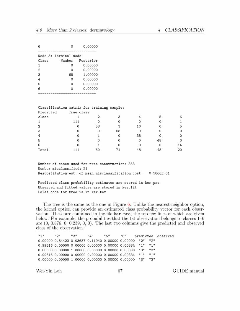
4.6 More than 2 classes: dermatology 4 CLASSIFICATION
6 0 0.00000
----------------------------
Node 3: Terminal node
Class Number Posterior
1 0 0.00000
2 0 0.00000
3 68 1.00000
4 0 0.00000
5 0 0.00000
6 0 0.00000
----------------------------
Classification matrix for training sample:
Predicted True class
class 1 2 3 4 5 6
1 111 0 0 0 0 1
2 0 58 3 10 0 5
3 0 0 68 0 0 0
4 0 1 0 38 0 0
5 0 0 0 0 48 0
6 0 1 0 0 0 14
Total 111 60 71 48 48 20
Number of cases used for tree construction: 358
Number misclassified: 21
Resubstitution est. of mean misclassification cost: 0.5866E-01
Predicted class probability estimates are stored in ker.pro
Observed and fitted values are stored in ker.fit
LaTeX code for tree is in ker.tex
The tree is the same as the one in Figure 6. Unlike the nearest-neighbor option,the kernel option can provide an estimated class probability vector for each obser-vation. These are contained in the file ker.pro, the top few lines of which are givenbelow. For example, the probabilities that the 1st observation belongs to classes 1–6are (0, 0.876, 0, 0.239, 0, 0). The last two columns give the predicted and observedclass of the observation.
"1" "2" "3" "4" "5" "6" predicted observed
0.00000 0.84423 0.03637 0.11940 0.00000 0.00000 "2" "2"
0.99616 0.00000 0.00000 0.00000 0.00000 0.00384 "1" "1"
0.00000 0.00000 1.00000 0.00000 0.00000 0.00000 "3" "3"
0.99616 0.00000 0.00000 0.00000 0.00000 0.00384 "1" "1"
0.00000 0.00000 1.00000 0.00000 0.00000 0.00000 "3" "3"
Wei-Yin Loh 67 GUIDE manual
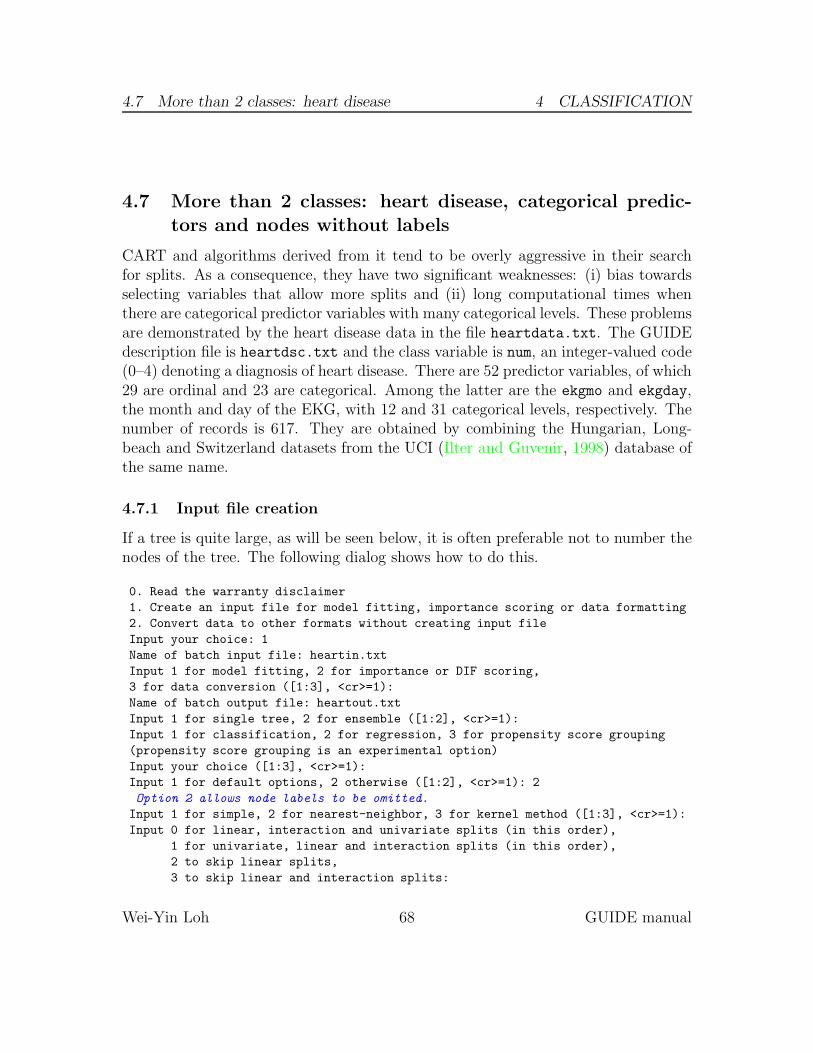
4.7 More than 2 classes: heart disease 4 CLASSIFICATION
4.7 More than 2 classes: heart disease, categorical predic-tors and nodes without labels
CART and algorithms derived from it tend to be overly aggressive in their searchfor splits. As a consequence, they have two significant weaknesses: (i) bias towardsselecting variables that allow more splits and (ii) long computational times whenthere are categorical predictor variables with many categorical levels. These problemsare demonstrated by the heart disease data in the file heartdata.txt. The GUIDEdescription file is heartdsc.txt and the class variable is num, an integer-valued code(0–4) denoting a diagnosis of heart disease. There are 52 predictor variables, of which29 are ordinal and 23 are categorical. Among the latter are the ekgmo and ekgday,the month and day of the EKG, with 12 and 31 categorical levels, respectively. Thenumber of records is 617. They are obtained by combining the Hungarian, Long-beach and Switzerland datasets from the UCI (Ilter and Guvenir, 1998) database ofthe same name.
4.7.1 Input file creation
If a tree is quite large, as will be seen below, it is often preferable not to number thenodes of the tree. The following dialog shows how to do this.
0. Read the warranty disclaimer
1. Create an input file for model fitting, importance scoring or data formatting
2. Convert data to other formats without creating input file
Input your choice: 1
Name of batch input file: heartin.txt
Input 1 for model fitting, 2 for importance or DIF scoring,
3 for data conversion ([1:3], <cr>=1):
Name of batch output file: heartout.txt
Input 1 for single tree, 2 for ensemble ([1:2], <cr>=1):
Input 1 for classification, 2 for regression, 3 for propensity score grouping
(propensity score grouping is an experimental option)
Input your choice ([1:3], <cr>=1):
Input 1 for default options, 2 otherwise ([1:2], <cr>=1): 2
Option 2 allows node labels to be omitted.
Input 1 for simple, 2 for nearest-neighbor, 3 for kernel method ([1:3], <cr>=1):
Input 0 for linear, interaction and univariate splits (in this order),
1 for univariate, linear and interaction splits (in this order),
2 to skip linear splits,
3 to skip linear and interaction splits:
Wei-Yin Loh 68 GUIDE manual
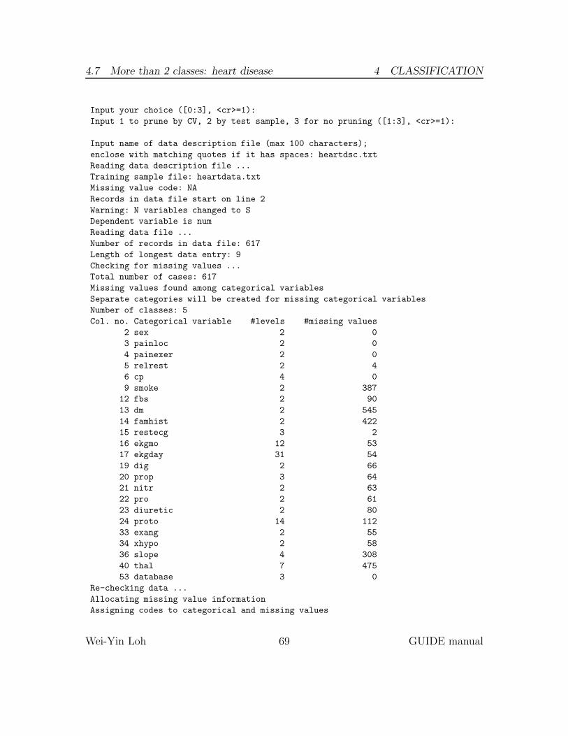
4.7 More than 2 classes: heart disease 4 CLASSIFICATION
Input your choice ([0:3], <cr>=1):
Input 1 to prune by CV, 2 by test sample, 3 for no pruning ([1:3], <cr>=1):
Input name of data description file (max 100 characters);
enclose with matching quotes if it has spaces: heartdsc.txt
Reading data description file ...
Training sample file: heartdata.txt
Missing value code: NA
Records in data file start on line 2
Warning: N variables changed to S
Dependent variable is num
Reading data file ...
Number of records in data file: 617
Length of longest data entry: 9
Checking for missing values ...
Total number of cases: 617
Missing values found among categorical variables
Separate categories will be created for missing categorical variables
Number of classes: 5
Col. no. Categorical variable #levels #missing values
2 sex 2 0
3 painloc 2 0
4 painexer 2 0
5 relrest 2 4
6 cp 4 0
9 smoke 2 387
12 fbs 2 90
13 dm 2 545
14 famhist 2 422
15 restecg 3 2
16 ekgmo 12 53
17 ekgday 31 54
19 dig 2 66
20 prop 3 64
21 nitr 2 63
22 pro 2 61
23 diuretic 2 80
24 proto 14 112
33 exang 2 55
34 xhypo 2 58
36 slope 4 308
40 thal 7 475
53 database 3 0
Re-checking data ...
Allocating missing value information
Assigning codes to categorical and missing values
Wei-Yin Loh 69 GUIDE manual
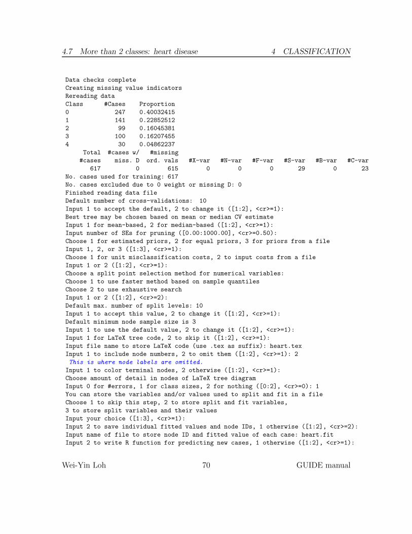
4.7 More than 2 classes: heart disease 4 CLASSIFICATION
Data checks complete
Creating missing value indicators
Rereading data
Class #Cases Proportion
0 247 0.40032415
1 141 0.22852512
2 99 0.16045381
3 100 0.16207455
4 30 0.04862237
Total #cases w/ #missing
#cases miss. D ord. vals #X-var #N-var #F-var #S-var #B-var #C-var
617 0 615 0 0 0 29 0 23
No. cases used for training: 617
No. cases excluded due to 0 weight or missing D: 0
Finished reading data file
Default number of cross-validations: 10
Input 1 to accept the default, 2 to change it ([1:2], <cr>=1):
Best tree may be chosen based on mean or median CV estimate
Input 1 for mean-based, 2 for median-based ([1:2], <cr>=1):
Input number of SEs for pruning ([0.00:1000.00], <cr>=0.50):
Choose 1 for estimated priors, 2 for equal priors, 3 for priors from a file
Input 1, 2, or 3 ([1:3], <cr>=1):
Choose 1 for unit misclassification costs, 2 to input costs from a file
Input 1 or 2 ([1:2], <cr>=1):
Choose a split point selection method for numerical variables:
Choose 1 to use faster method based on sample quantiles
Choose 2 to use exhaustive search
Input 1 or 2 ([1:2], <cr>=2):
Default max. number of split levels: 10
Input 1 to accept this value, 2 to change it ([1:2], <cr>=1):
Default minimum node sample size is 3
Input 1 to use the default value, 2 to change it ([1:2], <cr>=1):
Input 1 for LaTeX tree code, 2 to skip it ([1:2], <cr>=1):
Input file name to store LaTeX code (use .tex as suffix): heart.tex
Input 1 to include node numbers, 2 to omit them ([1:2], <cr>=1): 2
This is where node labels are omitted.
Input 1 to color terminal nodes, 2 otherwise ([1:2], <cr>=1):
Choose amount of detail in nodes of LaTeX tree diagram
Input 0 for #errors, 1 for class sizes, 2 for nothing ([0:2], <cr>=0): 1
You can store the variables and/or values used to split and fit in a file
Choose 1 to skip this step, 2 to store split and fit variables,
3 to store split variables and their values
Input your choice ([1:3], <cr>=1):
Input 2 to save individual fitted values and node IDs, 1 otherwise ([1:2], <cr>=2):
Input name of file to store node ID and fitted value of each case: heart.fit
Input 2 to write R function for predicting new cases, 1 otherwise ([1:2], <cr>=1):
Wei-Yin Loh 70 GUIDE manual

4.7 More than 2 classes: heart disease 4 CLASSIFICATION
Input file is created!
Run GUIDE with the command: guide < heartin.txt
Wei-Yin Loh 71 GUIDE manual

4.7
More
than2cla
sses:heart
disea
se4
CLASSIFIC
ATIO
N
lmt≤∗.5000
0.40
0.23
0.16
0.16
0.05
rcaprox
≤∗1.50
rcadist≤∗1.50
cxmain≤∗1.50
ladprox
≤∗1.50
laddist≤∗1.50
0.99
0.01
0.00
0.00
0.00
0190
16
0.00
1.00
0.00
0.00
0.00
115
0.00
0.87
0.13
0.00
0.00
laddist≤∗1.50
0.00
0.82
0.18
0.00
0.00
111
27
0.00
0.00
1.00
0.00
0.00
215
0.00
0.20
0.47
0.33
0.00
332
0.00
0.06
0.25
0.69
0.00
lmt≤ 1.50
rcaprox
≤∗1.50
rcadist≤∗1.50
ladprox
≤∗1.50
laddist≤∗1.50
cxmain≤∗1.50
0.92
0.08
0.00
0.00
0.00
063
120
0.00
1.00
0.00
0.00
0.00
cxmainramus
0.00
0.94
0.06
0.00
0.00
116
27
0.00
0.00
1.00
0.00
0.00
cxmain≤∗1.50
om1≤∗1.50
0.00
0.89
0.11
0.00
0.00
136
25
0.00
0.00
1.00
0.00
0.00
210
0.00
0.00
1.00
0.00
0.00
fbs= NA
0.00
0.67
0.22
0.11
0.00
19
317
0.00
0.06
0.12
0.82
0.00
ladprox
≤∗1.50
laddist≤∗1.50
cxmain≤∗1.50
0.00
0.93
0.07
0.00
0.00
129
218
0.00
0.00
1.00
0.00
0.00
318
0.00
0.00
0.17
0.83
0.00
cxmain≤∗1.50
ramus≤∗1.50
om1≤∗1.50
0.00
0.00
1.00
0.00
0.00
219
37
0.00
0.00
0.00
1.00
0.00
39
0.00
0.00
0.00
1.00
0.00
327
0.00
0.00
0.00
1.00
0.00
431
0.03
0.00
0.00
0.00
0.97
Figure 7: GUIDE v.27.9 0.50-SE classification tree for heart disease data
Wei-Y
inLoh
72GUID
Eman
ual

4.7 More than 2 classes: heart disease 4 CLASSIFICATION
4.7.2 Results
The GUIDE tree is shown in Figure 7 and the text output follows. Despite the treebeing quite large, no categorical variable is selected to split the nodes.
Classification tree
Pruning by cross-validation
Data description file: heartdsc.txt
Training sample file: heartdata.txt
Missing value code: NA
Records in data file start on line 2
Warning: N variables changed to S
Dependent variable is num
Number of records in data file: 617
Length of longest entry in data file: 9
Missing values found among categorical variables
Separate categories will be created for missing categorical variables
Number of classes: 5
Training sample class proportions of D variable num:
Class #Cases Proportion
0 247 0.40032415
1 141 0.22852512
2 99 0.16045381
3 100 0.16207455
4 30 0.04862237
Summary information (without x variables)
d=dependent, b=split and fit cat variable using 0-1 dummies,
c=split-only categorical, n=split and fit numerical, f=fit-only numerical,
s=split-only numerical, w=weight
Column Name Minimum Maximum #Categories #Missing
1 age s 2.8000E+01 7.7000E+01
2 sex c 2
3 painloc c 2
4 painexer c 2
5 relrest c 2 4
6 cp c 4
7 trestbps s 0.0000E+00 2.0000E+02 59
8 chol s 0.0000E+00 6.0300E+02 30
9 smoke c 2 387
10 cigs s 0.0000E+00 8.0000E+01 415
11 years s 0.0000E+00 6.0000E+01 427
12 fbs c 2 90
13 dm c 2 545
14 famhist c 2 422
15 restecg c 3 2
Wei-Yin Loh 73 GUIDE manual

4.7 More than 2 classes: heart disease 4 CLASSIFICATION
16 ekgmo c 12 53
17 ekgday c 31 54
18 ekgyr s 8.1000E+01 8.7000E+01 53
19 dig c 2 66
20 prop c 3 64
21 nitr c 2 63
22 pro c 2 61
23 diuretic c 2 80
24 proto c 14 112
25 thaldur s 1.0000E+00 2.4000E+01 56
26 thaltime s 0.0000E+00 2.0000E+01 384
27 met s 2.0000E+00 2.0000E+02 105
28 thalach s 6.0000E+01 1.9000E+02 55
29 thalrest s 3.7000E+01 1.3900E+02 56
30 tpeakbps s 1.0000E+02 2.4000E+02 63
31 tpeakbpd s 1.1000E+01 1.3400E+02 63
32 trestbpd s 0.0000E+00 1.2000E+02 59
33 exang c 2 55
34 xhypo c 2 58
35 oldpeak s -2.6000E+00 5.0000E+00 62
36 slope c 4 308
37 rldv5 s 2.0000E+00 3.6000E+01 143
38 rldv5e s 2.0000E+00 3.6000E+01 142
39 ca s 0.0000E+00 9.0000E+00 606
40 thal c 7 475
41 cyr s 1.0000E+00 8.7000E+01 9
42 num d 5
43 lmt s 0.0000E+00 1.6200E+02 275
44 ladprox s 1.0000E+00 2.0000E+00 236
45 laddist s 1.0000E+00 2.0000E+00 246
46 diag s 1.0000E+00 2.0000E+00 276
47 cxmain s 1.0000E+00 2.0000E+00 235
48 ramus s 1.0000E+00 2.0000E+00 285
49 om1 s 1.0000E+00 2.0000E+00 271
50 om2 s 1.0000E+00 2.0000E+00 290
51 rcaprox s 1.0000E+00 2.0000E+00 245
52 rcadist s 1.0000E+00 2.0000E+00 270
53 database c 3
Total #cases w/ #missing
#cases miss. D ord. vals #X-var #N-var #F-var #S-var #B-var #C-var
617 0 615 0 0 0 29 0 23
No. cases used for training: 617
No. cases excluded due to 0 weight or missing D: 0
Univariate split highest priority
Wei-Yin Loh 74 GUIDE manual
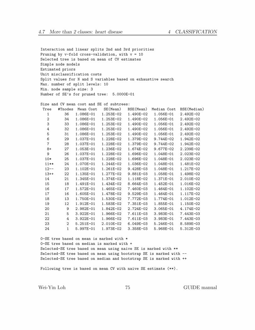
4.7 More than 2 classes: heart disease 4 CLASSIFICATION
Interaction and linear splits 2nd and 3rd priorities
Pruning by v-fold cross-validation, with v = 10
Selected tree is based on mean of CV estimates
Simple node models
Estimated priors
Unit misclassification costs
Split values for N and S variables based on exhaustive search
Max. number of split levels: 10
Min. node sample size: 3
Number of SE’s for pruned tree: 5.0000E-01
Size and CV mean cost and SE of subtrees:
Tree #Tnodes Mean Cost SE(Mean) BSE(Mean) Median Cost BSE(Median)
1 36 1.086E-01 1.253E-02 1.490E-02 1.056E-01 2.492E-02
2 34 1.086E-01 1.253E-02 1.490E-02 1.056E-01 2.492E-02
3 33 1.086E-01 1.253E-02 1.490E-02 1.056E-01 2.492E-02
4 32 1.086E-01 1.253E-02 1.490E-02 1.056E-01 2.492E-02
5 31 1.086E-01 1.253E-02 1.490E-02 1.056E-01 2.492E-02
6 29 1.037E-01 1.228E-02 1.379E-02 9.744E-02 1.942E-02
7 28 1.037E-01 1.228E-02 1.379E-02 9.744E-02 1.942E-02
8+ 27 1.053E-01 1.236E-02 1.674E-02 9.677E-02 2.239E-02
9 26 1.037E-01 1.228E-02 1.696E-02 1.048E-01 2.023E-02
10* 25 1.037E-01 1.228E-02 1.696E-02 1.048E-01 2.023E-02
11** 24 1.070E-01 1.244E-02 1.036E-02 1.048E-01 1.481E-02
12-- 23 1.102E-01 1.261E-02 9.428E-03 1.048E-01 1.217E-02
13++ 22 1.135E-01 1.277E-02 9.881E-03 1.058E-01 1.498E-02
14 21 1.345E-01 1.374E-02 1.118E-02 1.371E-01 2.010E-02
15 18 1.491E-01 1.434E-02 8.664E-03 1.452E-01 1.016E-02
16 17 1.572E-01 1.465E-02 7.460E-03 1.464E-01 1.102E-02
17 16 1.605E-01 1.478E-02 9.529E-03 1.464E-01 1.117E-02
18 13 1.750E-01 1.530E-02 7.772E-03 1.774E-01 1.012E-02
19 12 1.912E-01 1.583E-02 7.351E-03 1.855E-01 1.150E-02
20 9 2.982E-01 1.842E-02 2.724E-02 3.065E-01 4.174E-02
21 5 3.922E-01 1.966E-02 7.611E-03 3.983E-01 7.443E-03
22 4 3.922E-01 1.966E-02 7.611E-03 3.983E-01 7.443E-03
23 2 5.251E-01 2.010E-02 6.049E-03 5.246E-01 8.589E-03
24 1 5.997E-01 1.973E-02 3.358E-03 5.968E-01 5.312E-03
0-SE tree based on mean is marked with *
0-SE tree based on median is marked with +
Selected-SE tree based on mean using naive SE is marked with **
Selected-SE tree based on mean using bootstrap SE is marked with --
Selected-SE tree based on median and bootstrap SE is marked with ++
Following tree is based on mean CV with naive SE estimate (**).
Wei-Yin Loh 75 GUIDE manual
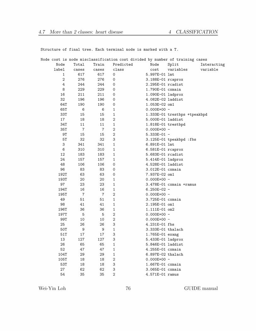
4.7 More than 2 classes: heart disease 4 CLASSIFICATION
Structure of final tree. Each terminal node is marked with a T.
Node cost is node misclassification cost divided by number of training cases
Node Total Train Predicted Node Split Interacting
label cases cases class cost variables variable
1 617 617 0 5.997E-01 lmt
2 276 276 0 3.188E-01 rcaprox
4 244 244 0 2.295E-01 rcadist
8 229 229 0 1.790E-01 cxmain
16 211 211 0 1.090E-01 ladprox
32 196 196 0 4.082E-02 laddist
64T 190 190 0 1.053E-02 om1
65T 6 6 1 0.000E+00 -
33T 15 15 1 1.333E-01 trestbps +tpeakbpd
17 18 18 2 5.000E-01 laddist
34T 11 11 1 1.818E-01 trestbpd
35T 7 7 2 0.000E+00 -
9T 15 15 2 5.333E-01 -
5T 32 32 3 3.125E-01 tpeakbpd :fbs
3 341 341 1 6.891E-01 lmt
6 310 310 1 6.581E-01 rcaprox
12 183 183 1 5.683E-01 rcadist
24 157 157 1 5.414E-01 ladprox
48 106 106 0 4.528E-01 laddist
96 83 83 0 3.012E-01 cxmain
192T 63 63 0 7.937E-02 om1
193T 20 20 1 0.000E+00 -
97 23 23 1 3.478E-01 cxmain +ramus
194T 16 16 1 6.250E-02 -
195T 7 7 2 0.000E+00 -
49 51 51 1 3.725E-01 cxmain
98 41 41 1 2.195E-01 om1
196T 36 36 1 1.111E-01 om2
197T 5 5 2 0.000E+00 -
99T 10 10 2 0.000E+00 -
25 26 26 3 4.231E-01 fbs
50T 9 9 1 3.333E-01 thalach
51T 17 17 3 1.765E-01 exang
13 127 127 3 5.433E-01 ladprox
26 65 65 1 5.846E-01 laddist
52 47 47 1 4.255E-01 cxmain
104T 29 29 1 6.897E-02 thalach
105T 18 18 2 0.000E+00 -
53T 18 18 3 1.667E-01 cxmain
27 62 62 3 3.065E-01 cxmain
54 35 35 2 4.571E-01 ramus
Wei-Yin Loh 76 GUIDE manual

4.7 More than 2 classes: heart disease 4 CLASSIFICATION
108 26 26 2 2.692E-01 om1
216T 19 19 2 0.000E+00 -
217T 7 7 3 0.000E+00 -
109T 9 9 3 0.000E+00 -
55T 27 27 3 0.000E+00 -
7T 31 31 4 3.226E-02 -
Warning: tree very large, omitting node numbers in LaTeX file
Number of terminal nodes of final tree: 24
Total number of nodes of final tree: 47
Second best split variable (based on curvature test) at root node is rcaprox
Classification tree:
At each categorical variable split, values not in training data go right
Node 1: lmt <= 0.50000 or NA
Node 2: rcaprox <= 1.50000 or NA
Node 4: rcadist <= 1.50000 or NA
Node 8: cxmain <= 1.50000 or NA
Node 16: ladprox <= 1.50000 or NA
Node 32: laddist <= 1.50000 or NA
Node 64: 0
Node 32: laddist > 1.50000
Node 65: 1
Node 16: ladprox > 1.50000
Node 33: 1
Node 8: cxmain > 1.50000
Node 17: laddist <= 1.50000 or NA
Node 34: 1
Node 17: laddist > 1.50000
Node 35: 2
Node 4: rcadist > 1.50000
Node 9: 2
Node 2: rcaprox > 1.50000
Node 5: 3
Node 1: lmt > 0.50000
Node 3: lmt <= 1.50000
Node 6: rcaprox <= 1.50000 or NA
Node 12: rcadist <= 1.50000 or NA
Node 24: ladprox <= 1.50000 or NA
Node 48: laddist <= 1.50000 or NA
Node 96: cxmain <= 1.50000 or NA
Node 192: 0
Node 96: cxmain > 1.50000
Node 193: 1
Node 48: laddist > 1.50000
Wei-Yin Loh 77 GUIDE manual
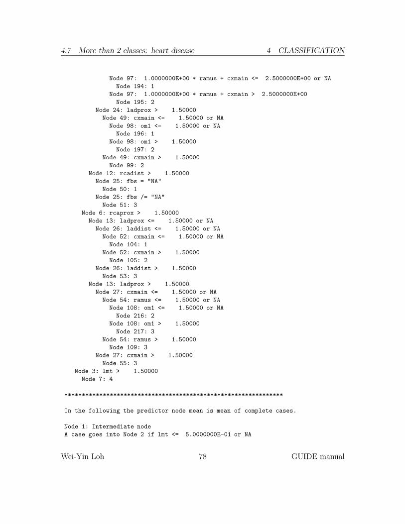
4.7 More than 2 classes: heart disease 4 CLASSIFICATION
Node 97: 1.0000000E+00 * ramus + cxmain <= 2.5000000E+00 or NA
Node 194: 1
Node 97: 1.0000000E+00 * ramus + cxmain > 2.5000000E+00
Node 195: 2
Node 24: ladprox > 1.50000
Node 49: cxmain <= 1.50000 or NA
Node 98: om1 <= 1.50000 or NA
Node 196: 1
Node 98: om1 > 1.50000
Node 197: 2
Node 49: cxmain > 1.50000
Node 99: 2
Node 12: rcadist > 1.50000
Node 25: fbs = "NA"
Node 50: 1
Node 25: fbs /= "NA"
Node 51: 3
Node 6: rcaprox > 1.50000
Node 13: ladprox <= 1.50000 or NA
Node 26: laddist <= 1.50000 or NA
Node 52: cxmain <= 1.50000 or NA
Node 104: 1
Node 52: cxmain > 1.50000
Node 105: 2
Node 26: laddist > 1.50000
Node 53: 3
Node 13: ladprox > 1.50000
Node 27: cxmain <= 1.50000 or NA
Node 54: ramus <= 1.50000 or NA
Node 108: om1 <= 1.50000 or NA
Node 216: 2
Node 108: om1 > 1.50000
Node 217: 3
Node 54: ramus > 1.50000
Node 109: 3
Node 27: cxmain > 1.50000
Node 55: 3
Node 3: lmt > 1.50000
Node 7: 4
***************************************************************
In the following the predictor node mean is mean of complete cases.
Node 1: Intermediate node
A case goes into Node 2 if lmt <= 5.0000000E-01 or NA
Wei-Yin Loh 78 GUIDE manual
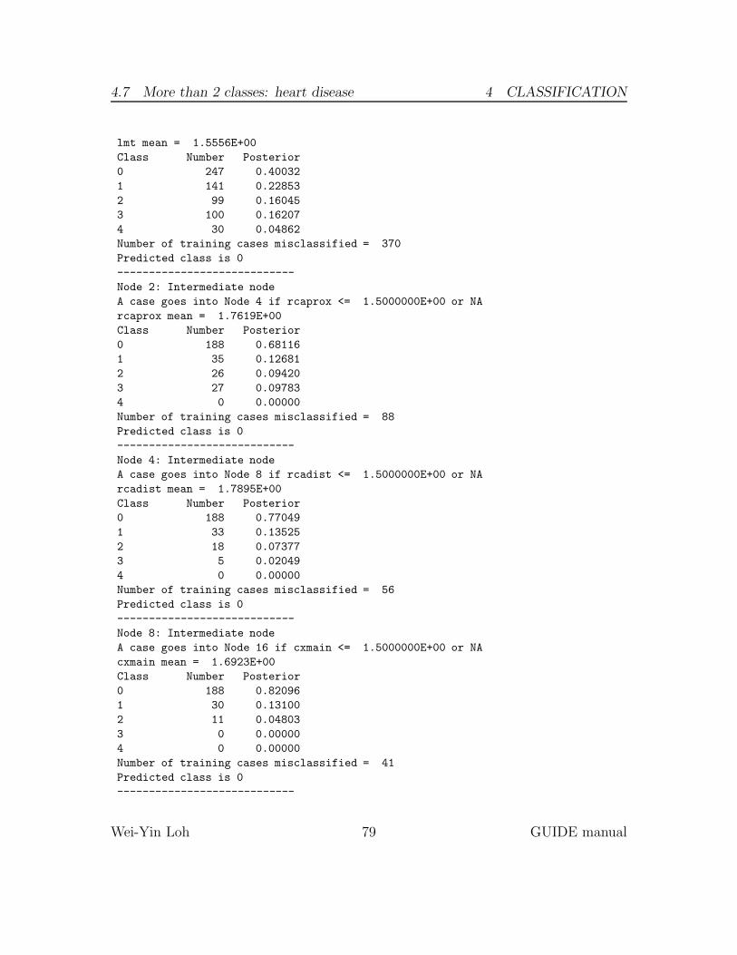
4.7 More than 2 classes: heart disease 4 CLASSIFICATION
lmt mean = 1.5556E+00
Class Number Posterior
0 247 0.40032
1 141 0.22853
2 99 0.16045
3 100 0.16207
4 30 0.04862
Number of training cases misclassified = 370
Predicted class is 0
----------------------------
Node 2: Intermediate node
A case goes into Node 4 if rcaprox <= 1.5000000E+00 or NA
rcaprox mean = 1.7619E+00
Class Number Posterior
0 188 0.68116
1 35 0.12681
2 26 0.09420
3 27 0.09783
4 0 0.00000
Number of training cases misclassified = 88
Predicted class is 0
----------------------------
Node 4: Intermediate node
A case goes into Node 8 if rcadist <= 1.5000000E+00 or NA
rcadist mean = 1.7895E+00
Class Number Posterior
0 188 0.77049
1 33 0.13525
2 18 0.07377
3 5 0.02049
4 0 0.00000
Number of training cases misclassified = 56
Predicted class is 0
----------------------------
Node 8: Intermediate node
A case goes into Node 16 if cxmain <= 1.5000000E+00 or NA
cxmain mean = 1.6923E+00
Class Number Posterior
0 188 0.82096
1 30 0.13100
2 11 0.04803
3 0 0.00000
4 0 0.00000
Number of training cases misclassified = 41
Predicted class is 0
----------------------------
Wei-Yin Loh 79 GUIDE manual

4.7 More than 2 classes: heart disease 4 CLASSIFICATION
Node 16: Intermediate node
A case goes into Node 32 if ladprox <= 1.5000000E+00 or NA
ladprox mean = 1.6818E+00
Class Number Posterior
0 188 0.89100
1 21 0.09953
2 2 0.00948
3 0 0.00000
4 0 0.00000
Number of training cases misclassified = 23
Predicted class is 0
----------------------------
Node 32: Intermediate node
A case goes into Node 64 if laddist <= 1.5000000E+00 or NA
laddist mean = 1.2857E+00
Class Number Posterior
0 188 0.95918
1 8 0.04082
2 0 0.00000
3 0 0.00000
4 0 0.00000
Number of training cases misclassified = 8
Predicted class is 0
----------------------------
Node 64: Terminal node
Class Number Posterior
0 188 0.98947
1 2 0.01053
2 0 0.00000
3 0 0.00000
4 0 0.00000
Number of training cases misclassified = 2
Predicted class is 0
----------------------------
Node 65: Terminal node
Class Number Posterior
0 0 0.00000
1 6 1.00000
2 0 0.00000
3 0 0.00000
4 0 0.00000
Number of training cases misclassified = 0
Predicted class is 1
----------------------------
Node 33: Terminal node
Class Number Posterior
Wei-Yin Loh 80 GUIDE manual
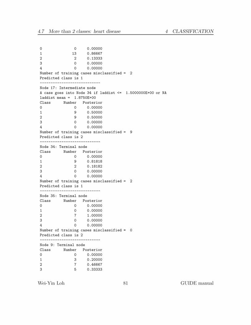
4.7 More than 2 classes: heart disease 4 CLASSIFICATION
0 0 0.00000
1 13 0.86667
2 2 0.13333
3 0 0.00000
4 0 0.00000
Number of training cases misclassified = 2
Predicted class is 1
----------------------------
Node 17: Intermediate node
A case goes into Node 34 if laddist <= 1.5000000E+00 or NA
laddist mean = 1.8750E+00
Class Number Posterior
0 0 0.00000
1 9 0.50000
2 9 0.50000
3 0 0.00000
4 0 0.00000
Number of training cases misclassified = 9
Predicted class is 2
----------------------------
Node 34: Terminal node
Class Number Posterior
0 0 0.00000
1 9 0.81818
2 2 0.18182
3 0 0.00000
4 0 0.00000
Number of training cases misclassified = 2
Predicted class is 1
----------------------------
Node 35: Terminal node
Class Number Posterior
0 0 0.00000
1 0 0.00000
2 7 1.00000
3 0 0.00000
4 0 0.00000
Number of training cases misclassified = 0
Predicted class is 2
----------------------------
Node 9: Terminal node
Class Number Posterior
0 0 0.00000
1 3 0.20000
2 7 0.46667
3 5 0.33333
Wei-Yin Loh 81 GUIDE manual

4.7 More than 2 classes: heart disease 4 CLASSIFICATION
4 0 0.00000
Number of training cases misclassified = 8
Predicted class is 2
----------------------------
Node 5: Terminal node
Class Number Posterior
0 0 0.00000
1 2 0.06250
2 8 0.25000
3 22 0.68750
4 0 0.00000
Number of training cases misclassified = 10
Predicted class is 3
----------------------------
Node 3: Intermediate node
A case goes into Node 6 if lmt <= 1.5000000E+00
lmt mean = 1.5601E+00
Class Number Posterior
0 59 0.17302
1 106 0.31085
2 73 0.21408
3 73 0.21408
4 30 0.08798
Number of training cases misclassified = 235
Predicted class is 1
----------------------------
Node 6: Intermediate node
A case goes into Node 12 if rcaprox <= 1.5000000E+00 or NA
rcaprox mean = 1.4137E+00
Class Number Posterior
0 58 0.18710
1 106 0.34194
2 73 0.23548
3 73 0.23548
4 0 0.00000
Number of training cases misclassified = 204
Predicted class is 1
----------------------------
Node 12: Intermediate node
A case goes into Node 24 if rcadist <= 1.5000000E+00 or NA
rcadist mean = 1.1444E+00
Class Number Posterior
0 58 0.31694
1 79 0.43169
2 31 0.16940
3 15 0.08197
Wei-Yin Loh 82 GUIDE manual

4.7 More than 2 classes: heart disease 4 CLASSIFICATION
4 0 0.00000
Number of training cases misclassified = 104
Predicted class is 1
----------------------------
Node 24: Intermediate node
A case goes into Node 48 if ladprox <= 1.5000000E+00 or NA
ladprox mean = 1.3290E+00
Class Number Posterior
0 58 0.36943
1 72 0.45860
2 27 0.17197
3 0 0.00000
4 0 0.00000
Number of training cases misclassified = 85
Predicted class is 1
----------------------------
Node 48: Intermediate node
A case goes into Node 96 if laddist <= 1.5000000E+00 or NA
laddist mean = 1.2212E+00
Class Number Posterior
0 58 0.54717
1 40 0.37736
2 8 0.07547
3 0 0.00000
4 0 0.00000
Number of training cases misclassified = 48
Predicted class is 0
----------------------------
Node 96: Intermediate node
A case goes into Node 192 if cxmain <= 1.5000000E+00 or NA
cxmain mean = 1.2439E+00
Class Number Posterior
0 58 0.69880
1 25 0.30120
2 0 0.00000
3 0 0.00000
4 0 0.00000
Number of training cases misclassified = 25
Predicted class is 0
----------------------------
Node 192: Terminal node
Class Number Posterior
0 58 0.92063
1 5 0.07937
2 0 0.00000
3 0 0.00000
Wei-Yin Loh 83 GUIDE manual

4.7 More than 2 classes: heart disease 4 CLASSIFICATION
4 0 0.00000
Number of training cases misclassified = 5
Predicted class is 0
----------------------------
Node 193: Terminal node
Class Number Posterior
0 0 0.00000
1 20 1.00000
2 0 0.00000
3 0 0.00000
4 0 0.00000
Number of training cases misclassified = 0
Predicted class is 1
----------------------------
Node 97: Intermediate node
A case goes into Node 194 if
1.0000000E+00 * ramus + cxmain <= 2.5000000E+00 or NA
Linear combination mean = 2.3043E+00
Class Number Posterior
0 0 0.00000
1 15 0.65217
2 8 0.34783
3 0 0.00000
4 0 0.00000
Number of training cases misclassified = 8
Predicted class is 1
----------------------------
Node 194: Terminal node
Class Number Posterior
0 0 0.00000
1 15 0.93750
2 1 0.06250
3 0 0.00000
4 0 0.00000
Number of training cases misclassified = 1
Predicted class is 1
----------------------------
Node 195: Terminal node
Class Number Posterior
0 0 0.00000
1 0 0.00000
2 7 1.00000
3 0 0.00000
4 0 0.00000
Number of training cases misclassified = 0
Predicted class is 2
Wei-Yin Loh 84 GUIDE manual
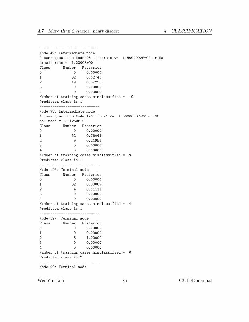
4.7 More than 2 classes: heart disease 4 CLASSIFICATION
----------------------------
Node 49: Intermediate node
A case goes into Node 98 if cxmain <= 1.5000000E+00 or NA
cxmain mean = 1.2000E+00
Class Number Posterior
0 0 0.00000
1 32 0.62745
2 19 0.37255
3 0 0.00000
4 0 0.00000
Number of training cases misclassified = 19
Predicted class is 1
----------------------------
Node 98: Intermediate node
A case goes into Node 196 if om1 <= 1.5000000E+00 or NA
om1 mean = 1.1250E+00
Class Number Posterior
0 0 0.00000
1 32 0.78049
2 9 0.21951
3 0 0.00000
4 0 0.00000
Number of training cases misclassified = 9
Predicted class is 1
----------------------------
Node 196: Terminal node
Class Number Posterior
0 0 0.00000
1 32 0.88889
2 4 0.11111
3 0 0.00000
4 0 0.00000
Number of training cases misclassified = 4
Predicted class is 1
----------------------------
Node 197: Terminal node
Class Number Posterior
0 0 0.00000
1 0 0.00000
2 5 1.00000
3 0 0.00000
4 0 0.00000
Number of training cases misclassified = 0
Predicted class is 2
----------------------------
Node 99: Terminal node
Wei-Yin Loh 85 GUIDE manual
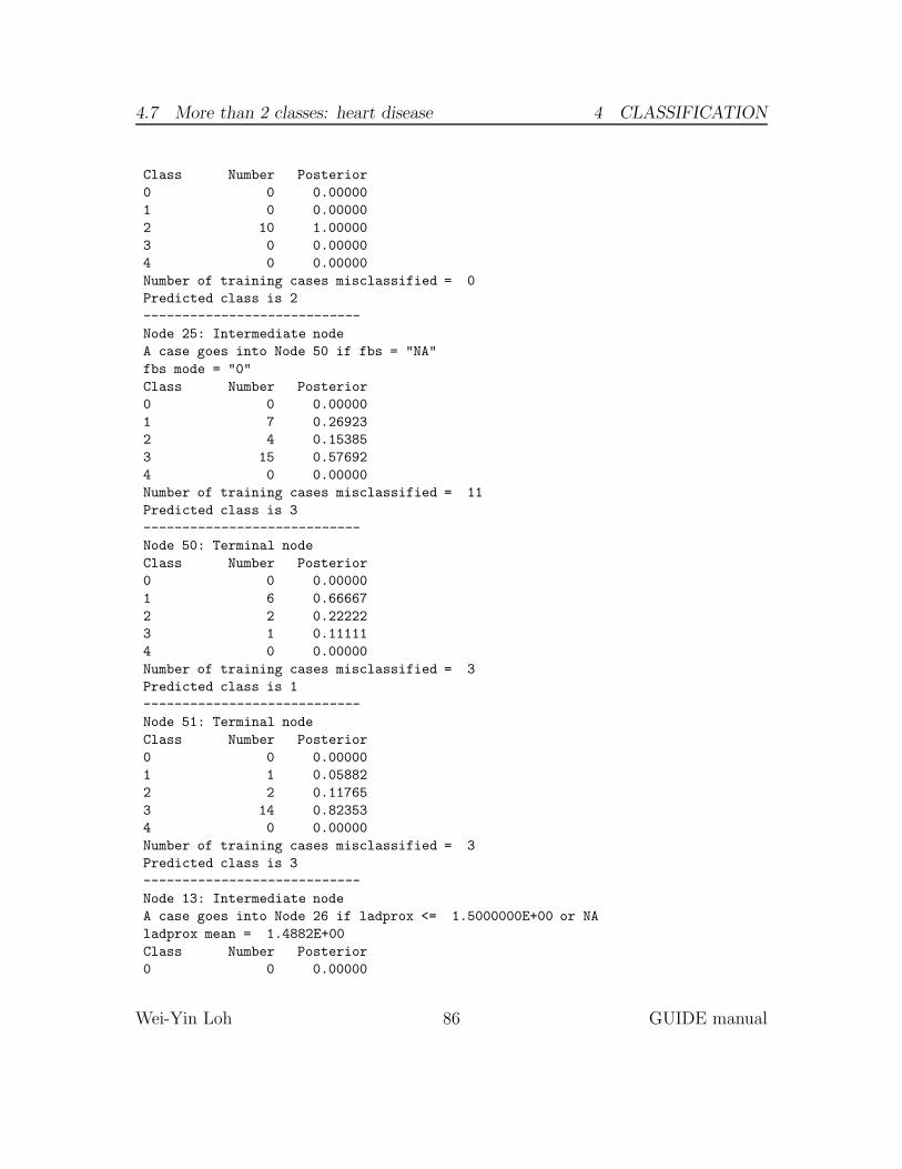
4.7 More than 2 classes: heart disease 4 CLASSIFICATION
Class Number Posterior
0 0 0.00000
1 0 0.00000
2 10 1.00000
3 0 0.00000
4 0 0.00000
Number of training cases misclassified = 0
Predicted class is 2
----------------------------
Node 25: Intermediate node
A case goes into Node 50 if fbs = "NA"
fbs mode = "0"
Class Number Posterior
0 0 0.00000
1 7 0.26923
2 4 0.15385
3 15 0.57692
4 0 0.00000
Number of training cases misclassified = 11
Predicted class is 3
----------------------------
Node 50: Terminal node
Class Number Posterior
0 0 0.00000
1 6 0.66667
2 2 0.22222
3 1 0.11111
4 0 0.00000
Number of training cases misclassified = 3
Predicted class is 1
----------------------------
Node 51: Terminal node
Class Number Posterior
0 0 0.00000
1 1 0.05882
2 2 0.11765
3 14 0.82353
4 0 0.00000
Number of training cases misclassified = 3
Predicted class is 3
----------------------------
Node 13: Intermediate node
A case goes into Node 26 if ladprox <= 1.5000000E+00 or NA
ladprox mean = 1.4882E+00
Class Number Posterior
0 0 0.00000
Wei-Yin Loh 86 GUIDE manual
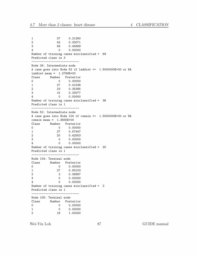
4.7 More than 2 classes: heart disease 4 CLASSIFICATION
1 27 0.21260
2 42 0.33071
3 58 0.45669
4 0 0.00000
Number of training cases misclassified = 69
Predicted class is 3
----------------------------
Node 26: Intermediate node
A case goes into Node 52 if laddist <= 1.5000000E+00 or NA
laddist mean = 1.2769E+00
Class Number Posterior
0 0 0.00000
1 27 0.41538
2 23 0.35385
3 15 0.23077
4 0 0.00000
Number of training cases misclassified = 38
Predicted class is 1
----------------------------
Node 52: Intermediate node
A case goes into Node 104 if cxmain <= 1.5000000E+00 or NA
cxmain mean = 1.3830E+00
Class Number Posterior
0 0 0.00000
1 27 0.57447
2 20 0.42553
3 0 0.00000
4 0 0.00000
Number of training cases misclassified = 20
Predicted class is 1
----------------------------
Node 104: Terminal node
Class Number Posterior
0 0 0.00000
1 27 0.93103
2 2 0.06897
3 0 0.00000
4 0 0.00000
Number of training cases misclassified = 2
Predicted class is 1
----------------------------
Node 105: Terminal node
Class Number Posterior
0 0 0.00000
1 0 0.00000
2 18 1.00000
Wei-Yin Loh 87 GUIDE manual
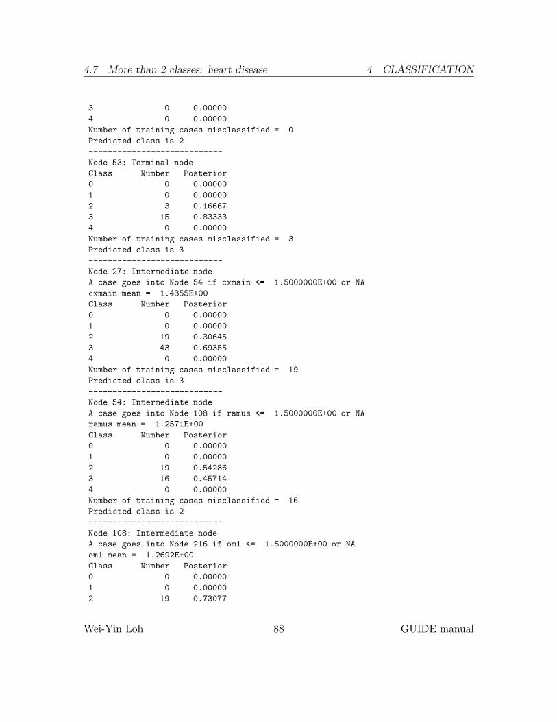
4.7 More than 2 classes: heart disease 4 CLASSIFICATION
3 0 0.00000
4 0 0.00000
Number of training cases misclassified = 0
Predicted class is 2
----------------------------
Node 53: Terminal node
Class Number Posterior
0 0 0.00000
1 0 0.00000
2 3 0.16667
3 15 0.83333
4 0 0.00000
Number of training cases misclassified = 3
Predicted class is 3
----------------------------
Node 27: Intermediate node
A case goes into Node 54 if cxmain <= 1.5000000E+00 or NA
cxmain mean = 1.4355E+00
Class Number Posterior
0 0 0.00000
1 0 0.00000
2 19 0.30645
3 43 0.69355
4 0 0.00000
Number of training cases misclassified = 19
Predicted class is 3
----------------------------
Node 54: Intermediate node
A case goes into Node 108 if ramus <= 1.5000000E+00 or NA
ramus mean = 1.2571E+00
Class Number Posterior
0 0 0.00000
1 0 0.00000
2 19 0.54286
3 16 0.45714
4 0 0.00000
Number of training cases misclassified = 16
Predicted class is 2
----------------------------
Node 108: Intermediate node
A case goes into Node 216 if om1 <= 1.5000000E+00 or NA
om1 mean = 1.2692E+00
Class Number Posterior
0 0 0.00000
1 0 0.00000
2 19 0.73077
Wei-Yin Loh 88 GUIDE manual
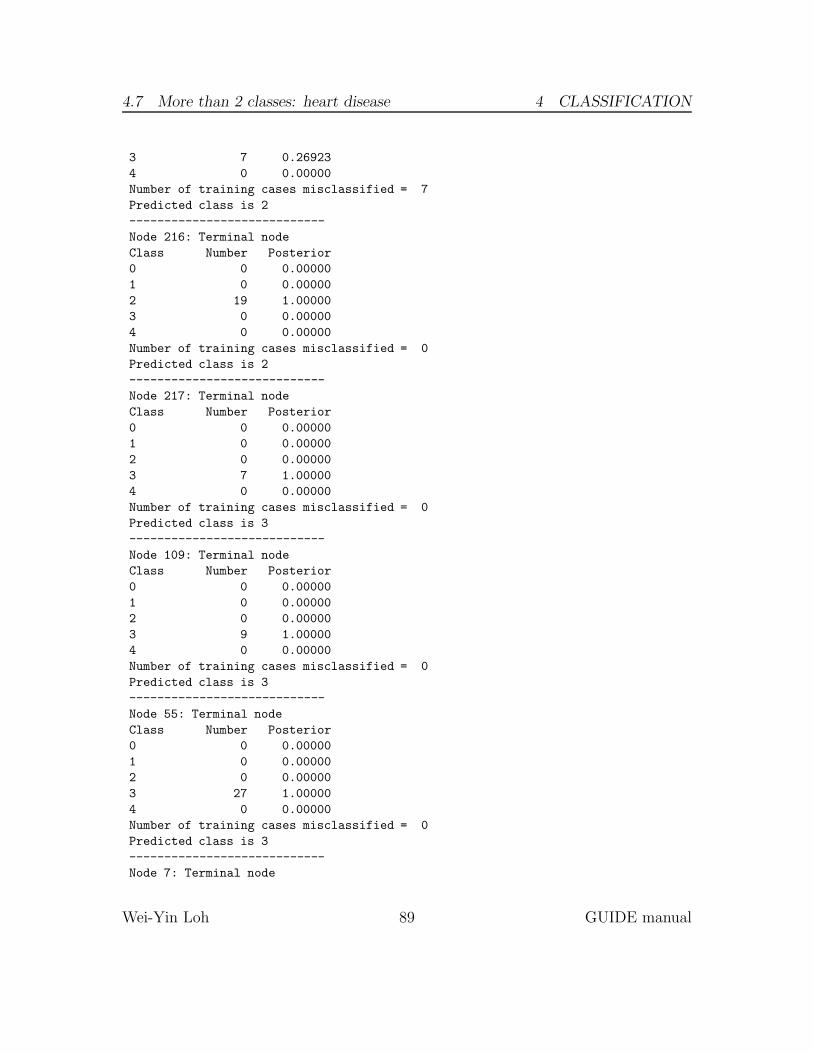
4.7 More than 2 classes: heart disease 4 CLASSIFICATION
3 7 0.26923
4 0 0.00000
Number of training cases misclassified = 7
Predicted class is 2
----------------------------
Node 216: Terminal node
Class Number Posterior
0 0 0.00000
1 0 0.00000
2 19 1.00000
3 0 0.00000
4 0 0.00000
Number of training cases misclassified = 0
Predicted class is 2
----------------------------
Node 217: Terminal node
Class Number Posterior
0 0 0.00000
1 0 0.00000
2 0 0.00000
3 7 1.00000
4 0 0.00000
Number of training cases misclassified = 0
Predicted class is 3
----------------------------
Node 109: Terminal node
Class Number Posterior
0 0 0.00000
1 0 0.00000
2 0 0.00000
3 9 1.00000
4 0 0.00000
Number of training cases misclassified = 0
Predicted class is 3
----------------------------
Node 55: Terminal node
Class Number Posterior
0 0 0.00000
1 0 0.00000
2 0 0.00000
3 27 1.00000
4 0 0.00000
Number of training cases misclassified = 0
Predicted class is 3
----------------------------
Node 7: Terminal node
Wei-Yin Loh 89 GUIDE manual

4.7 More than 2 classes: heart disease 4 CLASSIFICATION
Class Number Posterior
0 1 0.03226
1 0 0.00000
2 0 0.00000
3 0 0.00000
4 30 0.96774
Number of training cases misclassified = 1
Predicted class is 4
----------------------------
Classification matrix for training sample:
Predicted True class
class 0 1 2 3 4
0 246 7 0 0 0
1 0 128 13 1 0
2 0 3 73 5 0
3 0 3 13 94 0
4 1 0 0 0 30
Total 247 141 99 100 30
Number of cases used for tree construction: 617
Number misclassified: 46
Resubstitution est. of mean misclassification cost: 0.7455E-01
Observed and fitted values are stored in heart.fit
LaTeX code for tree is in heart.tex
4.7.3 RPART model
The GUIDE model in Figure 7 took 3 sec. to construct on a Linux computer. Incomparison, RPART (Therneau et al., 2017) took more than 3.5 hrs, due primarilyto the presence of the categorical variables ekgmo and ekgday. The result is shownin Figure 8. It splits repeatedly on ekgmo and ekgday.
Wei-Yin Loh 90 GUIDE manual

4.7
More
than2cla
sses:heart
disea
se4
CLASSIFIC
ATIO
N
|painexer=a
database=arcaprox< 1.5
ladprox< 1.5
cxmain< 1.5
lmt< 1.5
rcaprox< 1.5
ekgday=afghijkmnorstuvwxyBDE ladprox< 1.5
cxmain< 1.5
laddist< 1.5
ekgday=abcilmotA
database=a
oldpeak< 0.9
ekgday=djlmprvwCD
ekgday=bcefhnosxzABEekgmo=bcdehkl
ekgmo=beh
0247/141/99/100/30
0177/30/17/22/50
143/9/3/7/20
34/21/14/15/3
034/17/6/4/10
34/9/1/2/1034/4/1/0/1
10/5/0/2/0
10/8/5/2/0
30/4/8/11/2
170/111/82/78/25
125/85/59/58/0
125/62/25/11/0
119/58/10/9/0
26/4/15/2/0
30/23/34/47/0
10/23/19/10/0
10/23/5/4/01
0/23/2/0/03
0/0/3/4/0
20/0/14/6/0
30/0/15/37/02
0/0/12/6/03
0/0/3/31/0
045/26/23/20/25
044/26/23/20/13
034/9/7/4/2
110/17/16/16/11
11/14/3/1/2
39/3/13/15/92
9/3/12/12/13
7/2/1/10/106/2/0/2/0
31/0/1/8/1
22/1/11/2/0
40/0/1/3/8
41/0/0/0/12
Figure 8: RPART model for heart disease data
Wei-Y
inLoh
91GUID
Eman
ual

5 REGRESSION
5 Regression
GUIDE can fit least-squares (LS), quantile, Poisson, proportional hazards, and least-median-of-squares (LMS) regression tree models. We use the birthweight data in filesbirthwt.dat and birthwt.dsc to demonstrate LS models. The data consist of ob-servations from 50,000 live births. They are a subset of a larger dataset analyzedin Koenker and Hallock (2001); see also Koenker (2005). The variables are weight(infant birth weight), black (indicator of black mother), married (indicator of mar-ried mother), boy (indicator of boy), visit (prenatal visit: 0 = no visits, 1 = visitin 2nd trimester, 2 = visit in last trimester, 3 = visit in 1st trimester), ed (Mother’seducation level: 0 = high school, 1 = some college, 2 = college, 3 = less than highschool), smoke (indicator of smoking mother), cigsper (number of cigarettes smokedper day), age (mother’s age), and wtgain (mother’s weight gain during pregnancy).The contents of birthwt.dsc are:
birthwt.dat
NA
1
1 weight d
2 black c
3 married c
4 boy c
5 age n
6 smoke c
7 cigsper n
8 wtgain n
9 visit c
10 ed c
11 lowbwt x
The last variable lowbwt is a derived indicator of low birthweight not used here.
5.1 Least squares constant: birthwt data
5.1.1 Input file creation
The input file cons.in is obtained as follows. We select the non-default option toenable more selections to be provided.
0. Read the warranty disclaimer
1. Create a GUIDE input file
Input your choice: 1
Name of batch input file: cons.in
Input 1 for model fitting, 2 for importance or DIF scoring,
3 for data conversion ([1:3], <cr>=1):
Wei-Yin Loh 92 GUIDE manual
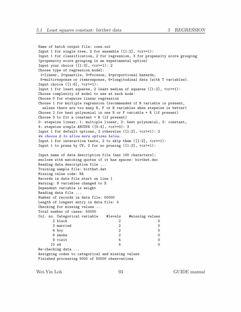
5.1 Least squares constant: birthwt data 5 REGRESSION
Name of batch output file: cons.out
Input 1 for single tree, 2 for ensemble ([1:2], <cr>=1):
Input 1 for classification, 2 for regression, 3 for propensity score grouping
(propensity score grouping is an experimental option)
Input your choice ([1:3], <cr>=1): 2
Choose type of regression model:
1=linear, 2=quantile, 3=Poisson, 4=proportional hazards,
5=multiresponse or itemresponse, 6=longitudinal data (with T variables).
Input choice ([1:6], <cr>=1):
Input 1 for least squares, 2 least median of squares ([1:2], <cr>=1):
Choose complexity of model to use at each node:
Choose 0 for stepwise linear regression
Choose 1 for multiple regression (recommended if R variable is present,
unless there are too many N, F or B variables when stepwise is better)
Choose 2 for best polynomial in one N or F variable + R (if present)
Choose 3 to fit a constant + R (if present)
0: stepwise linear, 1: multiple linear, 2: best polynomial, 3: constant,
4: stepwise simple ANCOVA ([0:4], <cr>=0): 3
Input 1 for default options, 2 otherwise ([1:2], <cr>=1): 2
We choose 2 to allow more options below.
Input 1 for interaction tests, 2 to skip them ([1:2], <cr>=1):
Input 1 to prune by CV, 2 for no pruning ([1:2], <cr>=1):
Input name of data description file (max 100 characters);
enclose with matching quotes if it has spaces: birthwt.dsc
Reading data description file ...
Training sample file: birthwt.dat
Missing value code: NA
Records in data file start on line 1
Warning: N variables changed to S
Dependent variable is weight
Reading data file ...
Number of records in data file: 50000
Length of longest entry in data file: 4
Checking for missing values ...
Total number of cases: 50000
Col. no. Categorical variable #levels #missing values
2 black 2 0
3 married 2 0
4 boy 2 0
6 smoke 2 0
9 visit 4 0
10 ed 4 0
Re-checking data ...
Assigning codes to categorical and missing values
Finished processing 5000 of 50000 observations
Wei-Yin Loh 93 GUIDE manual
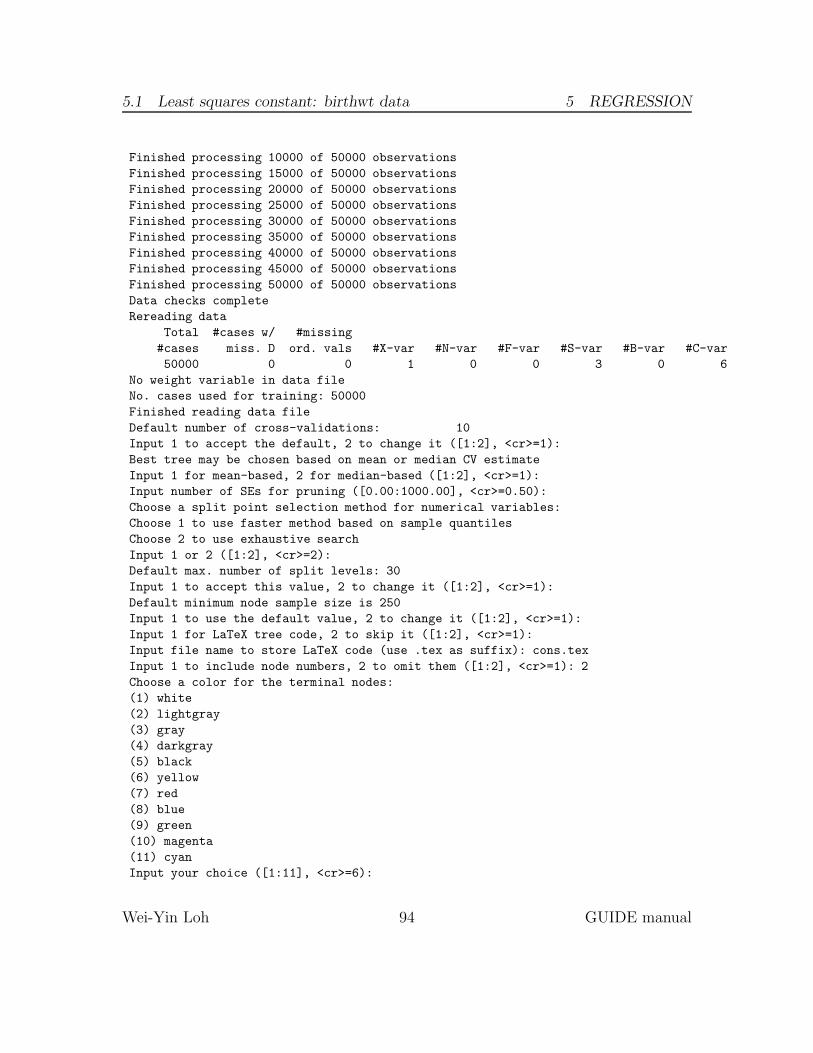
5.1 Least squares constant: birthwt data 5 REGRESSION
Finished processing 10000 of 50000 observations
Finished processing 15000 of 50000 observations
Finished processing 20000 of 50000 observations
Finished processing 25000 of 50000 observations
Finished processing 30000 of 50000 observations
Finished processing 35000 of 50000 observations
Finished processing 40000 of 50000 observations
Finished processing 45000 of 50000 observations
Finished processing 50000 of 50000 observations
Data checks complete
Rereading data
Total #cases w/ #missing
#cases miss. D ord. vals #X-var #N-var #F-var #S-var #B-var #C-var
50000 0 0 1 0 0 3 0 6
No weight variable in data file
No. cases used for training: 50000
Finished reading data file
Default number of cross-validations: 10
Input 1 to accept the default, 2 to change it ([1:2], <cr>=1):
Best tree may be chosen based on mean or median CV estimate
Input 1 for mean-based, 2 for median-based ([1:2], <cr>=1):
Input number of SEs for pruning ([0.00:1000.00], <cr>=0.50):
Choose a split point selection method for numerical variables:
Choose 1 to use faster method based on sample quantiles
Choose 2 to use exhaustive search
Input 1 or 2 ([1:2], <cr>=2):
Default max. number of split levels: 30
Input 1 to accept this value, 2 to change it ([1:2], <cr>=1):
Default minimum node sample size is 250
Input 1 to use the default value, 2 to change it ([1:2], <cr>=1):
Input 1 for LaTeX tree code, 2 to skip it ([1:2], <cr>=1):
Input file name to store LaTeX code (use .tex as suffix): cons.tex
Input 1 to include node numbers, 2 to omit them ([1:2], <cr>=1): 2
Choose a color for the terminal nodes:
(1) white
(2) lightgray
(3) gray
(4) darkgray
(5) black
(6) yellow
(7) red
(8) blue
(9) green
(10) magenta
(11) cyan
Input your choice ([1:11], <cr>=6):
Wei-Yin Loh 94 GUIDE manual
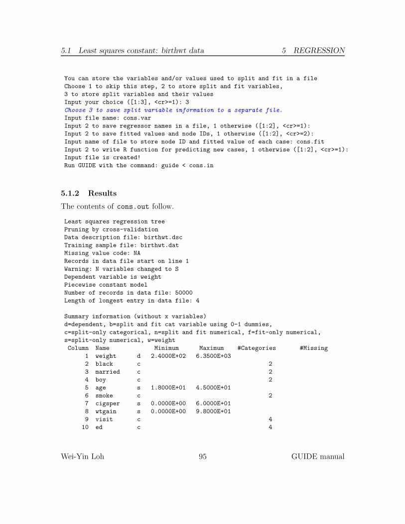
5.1 Least squares constant: birthwt data 5 REGRESSION
You can store the variables and/or values used to split and fit in a file
Choose 1 to skip this step, 2 to store split and fit variables,
3 to store split variables and their values
Input your choice ([1:3], <cr>=1): 3
Choose 3 to save split variable information to a separate file.
Input file name: cons.var
Input 2 to save regressor names in a file, 1 otherwise ([1:2], <cr>=1):
Input 2 to save fitted values and node IDs, 1 otherwise ([1:2], <cr>=2):
Input name of file to store node ID and fitted value of each case: cons.fit
Input 2 to write R function for predicting new cases, 1 otherwise ([1:2], <cr>=1):
Input file is created!
Run GUIDE with the command: guide < cons.in
5.1.2 Results
The contents of cons.out follow.
Least squares regression tree
Pruning by cross-validation
Data description file: birthwt.dsc
Training sample file: birthwt.dat
Missing value code: NA
Records in data file start on line 1
Warning: N variables changed to S
Dependent variable is weight
Piecewise constant model
Number of records in data file: 50000
Length of longest entry in data file: 4
Summary information (without x variables)
d=dependent, b=split and fit cat variable using 0-1 dummies,
c=split-only categorical, n=split and fit numerical, f=fit-only numerical,
s=split-only numerical, w=weight
Column Name Minimum Maximum #Categories #Missing
1 weight d 2.4000E+02 6.3500E+03
2 black c 2
3 married c 2
4 boy c 2
5 age s 1.8000E+01 4.5000E+01
6 smoke c 2
7 cigsper s 0.0000E+00 6.0000E+01
8 wtgain s 0.0000E+00 9.8000E+01
9 visit c 4
10 ed c 4
Wei-Yin Loh 95 GUIDE manual

5.1 Least squares constant: birthwt data 5 REGRESSION
Total #cases w/ #missing
#cases miss. D ord. vals #X-var #N-var #F-var #S-var #B-var #C-var
50000 0 0 1 0 0 3 0 6
No weight variable in data file
No. cases used for training: 50000
Interaction tests on all variables
Pruning by v-fold cross-validation, with v = 10
Selected tree is based on mean of CV estimates
Split values for N and S variables based on exhaustive search
Max. number of split levels: 30
Min. node sample size: 250
Number of SE’s for pruned tree: 5.0000E-01
Size and CV MSE and SE of subtrees:
Tree #Tnodes Mean MSE SE(Mean) BSE(Mean) Median MSE BSE(Median)
1 147 2.891E+05 2.800E+03 1.678E+03 2.875E+05 2.016E+03
2 146 2.891E+05 2.800E+03 1.678E+03 2.875E+05 2.016E+03
3 145 2.891E+05 2.800E+03 1.678E+03 2.875E+05 2.016E+03
4 144 2.891E+05 2.800E+03 1.678E+03 2.875E+05 2.017E+03
5 143 2.891E+05 2.800E+03 1.678E+03 2.875E+05 2.017E+03
6 142 2.891E+05 2.800E+03 1.678E+03 2.875E+05 2.017E+03
7 141 2.891E+05 2.800E+03 1.678E+03 2.875E+05 2.017E+03
8 140 2.891E+05 2.800E+03 1.679E+03 2.875E+05 2.019E+03
9 139 2.891E+05 2.800E+03 1.678E+03 2.875E+05 2.022E+03
10 138 2.891E+05 2.800E+03 1.678E+03 2.875E+05 2.022E+03
11 137 2.891E+05 2.800E+03 1.679E+03 2.875E+05 2.026E+03
12 136 2.891E+05 2.800E+03 1.679E+03 2.875E+05 2.026E+03
13 135 2.891E+05 2.800E+03 1.679E+03 2.875E+05 2.026E+03
14 134 2.891E+05 2.800E+03 1.679E+03 2.875E+05 2.026E+03
15 133 2.891E+05 2.800E+03 1.679E+03 2.875E+05 2.026E+03
16 132 2.891E+05 2.800E+03 1.678E+03 2.875E+05 2.025E+03
17 131 2.891E+05 2.800E+03 1.681E+03 2.875E+05 2.018E+03
18 130 2.891E+05 2.800E+03 1.683E+03 2.875E+05 2.019E+03
19 129 2.891E+05 2.800E+03 1.681E+03 2.875E+05 2.023E+03
20 128 2.891E+05 2.800E+03 1.681E+03 2.875E+05 2.023E+03
21 127 2.891E+05 2.800E+03 1.680E+03 2.875E+05 2.019E+03
22 126 2.891E+05 2.800E+03 1.680E+03 2.875E+05 2.020E+03
23 125 2.891E+05 2.800E+03 1.680E+03 2.875E+05 2.020E+03
24 123 2.891E+05 2.800E+03 1.680E+03 2.875E+05 2.020E+03
25 122 2.891E+05 2.800E+03 1.680E+03 2.875E+05 2.020E+03
26 121 2.891E+05 2.800E+03 1.679E+03 2.875E+05 2.023E+03
27 119 2.891E+05 2.800E+03 1.679E+03 2.875E+05 2.024E+03
28 118 2.891E+05 2.800E+03 1.679E+03 2.875E+05 2.025E+03
29 117 2.891E+05 2.800E+03 1.679E+03 2.875E+05 2.025E+03
30 116 2.891E+05 2.800E+03 1.679E+03 2.875E+05 2.025E+03
Wei-Yin Loh 96 GUIDE manual
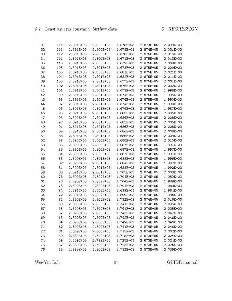
5.1 Least squares constant: birthwt data 5 REGRESSION
31 114 2.891E+05 2.800E+03 1.678E+03 2.874E+05 2.038E+03
32 113 2.891E+05 2.800E+03 1.678E+03 2.874E+05 2.031E+03
33 112 2.891E+05 2.800E+03 1.670E+03 2.875E+05 2.016E+03
34 111 2.891E+05 2.800E+03 1.671E+03 2.875E+05 2.013E+03
35 110 2.891E+05 2.800E+03 1.672E+03 2.875E+05 2.009E+03
36 108 2.891E+05 2.801E+03 1.678E+03 2.875E+05 2.009E+03
37 105 2.891E+05 2.800E+03 1.681E+03 2.875E+05 2.021E+03
38 104 2.891E+05 2.801E+03 1.682E+03 2.875E+05 2.011E+03
39 103 2.891E+05 2.801E+03 1.677E+03 2.875E+05 2.001E+03
40 102 2.891E+05 2.801E+03 1.676E+03 2.875E+05 2.002E+03
41 101 2.891E+05 2.801E+03 1.673E+03 2.876E+05 1.998E+03
42 99 2.891E+05 2.801E+03 1.674E+03 2.875E+05 1.995E+03
43 98 2.891E+05 2.801E+03 1.674E+03 2.875E+05 1.990E+03
44 97 2.891E+05 2.801E+03 1.674E+03 2.875E+05 1.990E+03
45 96 2.891E+05 2.801E+03 1.676E+03 2.875E+05 1.987E+03
46 95 2.891E+05 2.801E+03 1.685E+03 2.873E+05 2.005E+03
47 93 2.890E+05 2.801E+03 1.686E+03 2.873E+05 2.008E+03
48 92 2.891E+05 2.801E+03 1.685E+03 2.874E+05 2.005E+03
49 91 2.891E+05 2.801E+03 1.686E+03 2.874E+05 2.008E+03
50 89 2.891E+05 2.801E+03 1.686E+03 2.874E+05 2.008E+03
51 88 2.891E+05 2.801E+03 1.686E+03 2.874E+05 2.008E+03
52 87 2.890E+05 2.800E+03 1.688E+03 2.874E+05 2.010E+03
53 86 2.890E+05 2.800E+03 1.687E+03 2.874E+05 1.997E+03
54 85 2.890E+05 2.800E+03 1.687E+03 2.874E+05 1.997E+03
55 84 2.890E+05 2.800E+03 1.687E+03 2.874E+05 1.997E+03
56 83 2.890E+05 2.801E+03 1.688E+03 2.874E+05 1.996E+03
57 82 2.890E+05 2.801E+03 1.684E+03 2.874E+05 1.992E+03
58 81 2.890E+05 2.801E+03 1.688E+03 2.874E+05 1.992E+03
59 80 2.891E+05 2.801E+03 1.705E+03 2.874E+05 2.003E+03
60 78 2.890E+05 2.802E+03 1.704E+03 2.874E+05 1.989E+03
61 76 2.890E+05 2.802E+03 1.704E+03 2.874E+05 1.989E+03
62 75 2.890E+05 2.802E+03 1.704E+03 2.874E+05 1.989E+03
63 74 2.891E+05 2.802E+03 1.699E+03 2.874E+05 1.984E+03
64 72 2.891E+05 2.802E+03 1.699E+03 2.874E+05 1.984E+03
65 71 2.890E+05 2.802E+03 1.732E+03 2.874E+05 2.016E+03
66 69 2.890E+05 2.800E+03 1.741E+03 2.874E+05 2.035E+03
67 68 2.890E+05 2.800E+03 1.741E+03 2.874E+05 2.035E+03
68 67 2.890E+05 2.800E+03 1.743E+03 2.874E+05 2.047E+03
69 65 2.890E+05 2.800E+03 1.742E+03 2.874E+05 2.046E+03
70 64 2.890E+05 2.800E+03 1.742E+03 2.874E+05 2.046E+03
71 62 2.890E+05 2.800E+03 1.741E+03 2.874E+05 2.046E+03
72 61 2.889E+05 2.800E+03 1.715E+03 2.874E+05 2.002E+03
73 60 2.889E+05 2.799E+03 1.725E+03 2.873E+05 2.024E+03
74 59 2.889E+05 2.799E+03 1.725E+03 2.873E+05 2.024E+03
75 57 2.889E+05 2.799E+03 1.723E+03 2.873E+05 2.024E+03
76 55 2.889E+05 2.800E+03 1.732E+03 2.873E+05 2.039E+03
Wei-Yin Loh 97 GUIDE manual
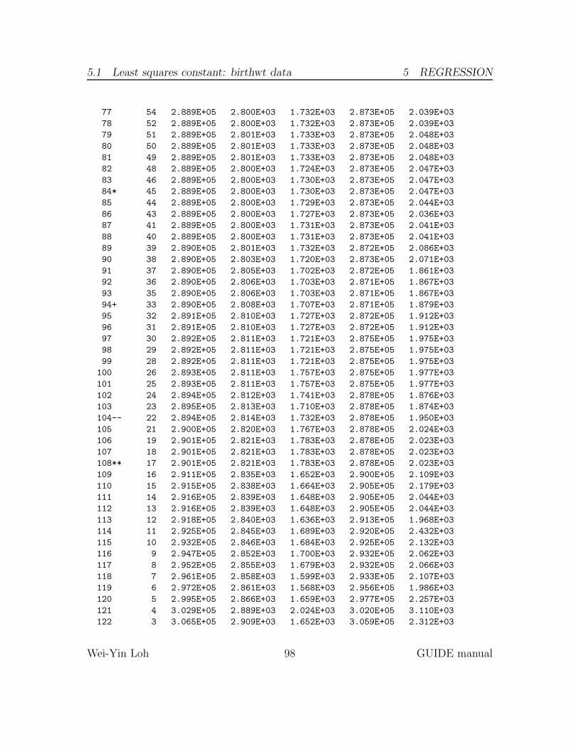
5.1 Least squares constant: birthwt data 5 REGRESSION
77 54 2.889E+05 2.800E+03 1.732E+03 2.873E+05 2.039E+03
78 52 2.889E+05 2.800E+03 1.732E+03 2.873E+05 2.039E+03
79 51 2.889E+05 2.801E+03 1.733E+03 2.873E+05 2.048E+03
80 50 2.889E+05 2.801E+03 1.733E+03 2.873E+05 2.048E+03
81 49 2.889E+05 2.801E+03 1.733E+03 2.873E+05 2.048E+03
82 48 2.889E+05 2.800E+03 1.724E+03 2.873E+05 2.047E+03
83 46 2.889E+05 2.800E+03 1.730E+03 2.873E+05 2.047E+03
84* 45 2.889E+05 2.800E+03 1.730E+03 2.873E+05 2.047E+03
85 44 2.889E+05 2.800E+03 1.729E+03 2.873E+05 2.044E+03
86 43 2.889E+05 2.800E+03 1.727E+03 2.873E+05 2.036E+03
87 41 2.889E+05 2.800E+03 1.731E+03 2.873E+05 2.041E+03
88 40 2.889E+05 2.800E+03 1.731E+03 2.873E+05 2.041E+03
89 39 2.890E+05 2.801E+03 1.732E+03 2.872E+05 2.086E+03
90 38 2.890E+05 2.803E+03 1.720E+03 2.873E+05 2.071E+03
91 37 2.890E+05 2.805E+03 1.702E+03 2.872E+05 1.861E+03
92 36 2.890E+05 2.806E+03 1.703E+03 2.871E+05 1.867E+03
93 35 2.890E+05 2.806E+03 1.703E+03 2.871E+05 1.867E+03
94+ 33 2.890E+05 2.808E+03 1.707E+03 2.871E+05 1.879E+03
95 32 2.891E+05 2.810E+03 1.727E+03 2.872E+05 1.912E+03
96 31 2.891E+05 2.810E+03 1.727E+03 2.872E+05 1.912E+03
97 30 2.892E+05 2.811E+03 1.721E+03 2.875E+05 1.975E+03
98 29 2.892E+05 2.811E+03 1.721E+03 2.875E+05 1.975E+03
99 28 2.892E+05 2.811E+03 1.721E+03 2.875E+05 1.975E+03
100 26 2.893E+05 2.811E+03 1.757E+03 2.875E+05 1.977E+03
101 25 2.893E+05 2.811E+03 1.757E+03 2.875E+05 1.977E+03
102 24 2.894E+05 2.812E+03 1.741E+03 2.878E+05 1.876E+03
103 23 2.895E+05 2.813E+03 1.710E+03 2.878E+05 1.874E+03
104-- 22 2.894E+05 2.814E+03 1.732E+03 2.878E+05 1.950E+03
105 21 2.900E+05 2.820E+03 1.767E+03 2.878E+05 2.024E+03
106 19 2.901E+05 2.821E+03 1.783E+03 2.878E+05 2.023E+03
107 18 2.901E+05 2.821E+03 1.783E+03 2.878E+05 2.023E+03
108** 17 2.901E+05 2.821E+03 1.783E+03 2.878E+05 2.023E+03
109 16 2.911E+05 2.835E+03 1.652E+03 2.900E+05 2.109E+03
110 15 2.915E+05 2.838E+03 1.664E+03 2.905E+05 2.179E+03
111 14 2.916E+05 2.839E+03 1.648E+03 2.905E+05 2.044E+03
112 13 2.916E+05 2.839E+03 1.648E+03 2.905E+05 2.044E+03
113 12 2.918E+05 2.840E+03 1.636E+03 2.913E+05 1.968E+03
114 11 2.925E+05 2.845E+03 1.689E+03 2.920E+05 2.432E+03
115 10 2.932E+05 2.846E+03 1.684E+03 2.925E+05 2.132E+03
116 9 2.947E+05 2.852E+03 1.700E+03 2.932E+05 2.062E+03
117 8 2.952E+05 2.855E+03 1.679E+03 2.932E+05 2.066E+03
118 7 2.961E+05 2.858E+03 1.599E+03 2.933E+05 2.107E+03
119 6 2.972E+05 2.861E+03 1.568E+03 2.956E+05 1.986E+03
120 5 2.995E+05 2.866E+03 1.659E+03 2.977E+05 2.257E+03
121 4 3.029E+05 2.889E+03 2.024E+03 3.020E+05 3.110E+03
122 3 3.065E+05 2.909E+03 1.652E+03 3.059E+05 2.312E+03
Wei-Yin Loh 98 GUIDE manual
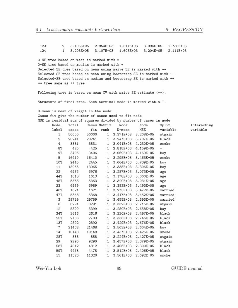
5.1 Least squares constant: birthwt data 5 REGRESSION
123 2 3.106E+05 2.954E+03 1.517E+03 3.094E+05 1.738E+03
124 1 3.208E+05 3.107E+03 1.608E+03 3.204E+05 2.111E+03
0-SE tree based on mean is marked with *
0-SE tree based on median is marked with +
Selected-SE tree based on mean using naive SE is marked with **
Selected-SE tree based on mean using bootstrap SE is marked with --
Selected-SE tree based on median and bootstrap SE is marked with ++
** tree same as ++ tree
Following tree is based on mean CV with naive SE estimate (**).
Structure of final tree. Each terminal node is marked with a T.
D-mean is mean of weight in the node
Cases fit give the number of cases used to fit node
MSE is residual sum of squares divided by number of cases in node
Node Total Cases Matrix Node Node Split Interacting
label cases fit rank D-mean MSE variable variable
1 50000 50000 1 3.371E+03 3.208E+05 wtgain
2 20241 20241 1 3.247E+03 3.707E+05 black
4 3831 3831 1 3.041E+03 4.230E+05 smoke
8T 425 425 1 2.818E+03 4.159E+05 -
9T 3406 3406 1 3.069E+03 4.169E+05 boy
5 16410 16410 1 3.295E+03 3.463E+05 smoke
10T 2445 2445 1 3.064E+03 3.739E+05 boy
11 13965 13965 1 3.335E+03 3.306E+05 boy
22 6976 6976 1 3.287E+03 3.073E+05 age
44T 1613 1613 1 3.178E+03 3.060E+05 age
45T 5363 5363 1 3.320E+03 3.031E+05 age
23 6989 6989 1 3.383E+03 3.493E+05 age
46T 1621 1621 1 3.273E+03 3.472E+05 married
47T 5368 5368 1 3.417E+03 3.452E+05 married
3 29759 29759 1 3.455E+03 2.693E+05 married
6 8291 8291 1 3.332E+03 2.715E+05 wtgain
12 5399 5399 1 3.280E+03 2.658E+05 boy
24T 2616 2616 1 3.220E+03 2.497E+05 black
25T 2783 2783 1 3.336E+03 2.746E+05 black
13T 2892 2892 1 3.429E+03 2.676E+05 black
7 21468 21468 1 3.503E+03 2.604E+05 boy
14 10148 10148 1 3.437E+03 2.425E+05 smoke
28T 858 858 1 3.224E+03 2.427E+05 wtgain
29 9290 9290 1 3.457E+03 2.379E+05 wtgain
58T 4812 4812 1 3.406E+03 2.300E+05 black
59T 4478 4478 1 3.512E+03 2.406E+05 black
15 11320 11320 1 3.561E+03 2.692E+05 smoke
Wei-Yin Loh 99 GUIDE manual
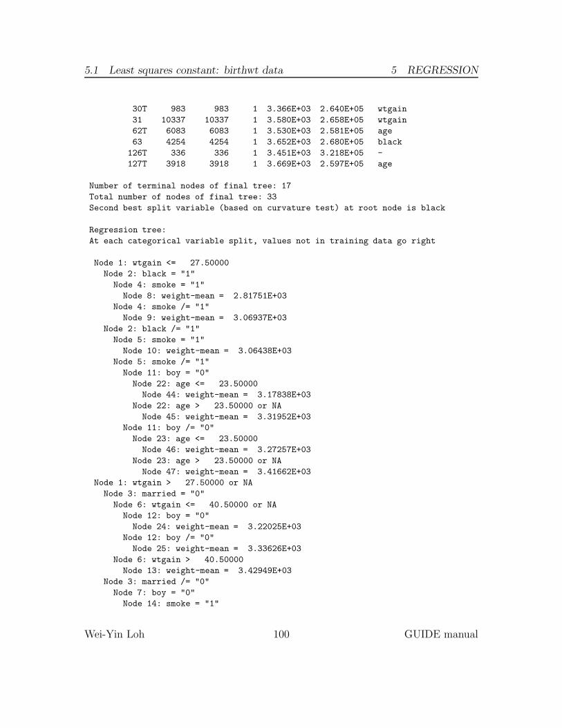
5.1 Least squares constant: birthwt data 5 REGRESSION
30T 983 983 1 3.366E+03 2.640E+05 wtgain
31 10337 10337 1 3.580E+03 2.658E+05 wtgain
62T 6083 6083 1 3.530E+03 2.581E+05 age
63 4254 4254 1 3.652E+03 2.680E+05 black
126T 336 336 1 3.451E+03 3.218E+05 -
127T 3918 3918 1 3.669E+03 2.597E+05 age
Number of terminal nodes of final tree: 17
Total number of nodes of final tree: 33
Second best split variable (based on curvature test) at root node is black
Regression tree:
At each categorical variable split, values not in training data go right
Node 1: wtgain <= 27.50000
Node 2: black = "1"
Node 4: smoke = "1"
Node 8: weight-mean = 2.81751E+03
Node 4: smoke /= "1"
Node 9: weight-mean = 3.06937E+03
Node 2: black /= "1"
Node 5: smoke = "1"
Node 10: weight-mean = 3.06438E+03
Node 5: smoke /= "1"
Node 11: boy = "0"
Node 22: age <= 23.50000
Node 44: weight-mean = 3.17838E+03
Node 22: age > 23.50000 or NA
Node 45: weight-mean = 3.31952E+03
Node 11: boy /= "0"
Node 23: age <= 23.50000
Node 46: weight-mean = 3.27257E+03
Node 23: age > 23.50000 or NA
Node 47: weight-mean = 3.41662E+03
Node 1: wtgain > 27.50000 or NA
Node 3: married = "0"
Node 6: wtgain <= 40.50000 or NA
Node 12: boy = "0"
Node 24: weight-mean = 3.22025E+03
Node 12: boy /= "0"
Node 25: weight-mean = 3.33626E+03
Node 6: wtgain > 40.50000
Node 13: weight-mean = 3.42949E+03
Node 3: married /= "0"
Node 7: boy = "0"
Node 14: smoke = "1"
Wei-Yin Loh 100 GUIDE manual

5.1 Least squares constant: birthwt data 5 REGRESSION
Node 28: weight-mean = 3.22371E+03
Node 14: smoke /= "1"
Node 29: wtgain <= 35.50000 or NA
Node 58: weight-mean = 3.40565E+03
Node 29: wtgain > 35.50000
Node 59: weight-mean = 3.51164E+03
Node 7: boy /= "0"
Node 15: smoke = "1"
Node 30: weight-mean = 3.36637E+03
Node 15: smoke /= "1"
Node 31: wtgain <= 38.50000 or NA
Node 62: weight-mean = 3.52951E+03
Node 31: wtgain > 38.50000
Node 63: black = "1"
Node 126: weight-mean = 3.45097E+03
Node 63: black /= "1"
Node 127: weight-mean = 3.66879E+03
***************************************************************
WARNING: p-values below are not adjusted for split search. For a bootstrap
solution, see Loh et al. (2016), "Identification of subgroups with
differential treatment effects for longitudinal and multiresponse
variables", Statistics in Medicine, v.35, 4837-4855.
Node 1: Intermediate node
A case goes into Node 2 if wtgain <= 2.7500000E+01
wtgain mean = 3.0709E+01
Coefficients of least squares regression function:
Regressor Coefficient t-stat p-val
Constant 3.3708E+03 1330.76 0.0000
Mean of weight = 3370.7566400000001
----------------------------
Node 2: Intermediate node
A case goes into Node 4 if black = "1"
black mode = "0"
----------------------------
Node 4: Intermediate node
A case goes into Node 8 if smoke = "1"
smoke mode = "0"
----------------------------
Node 8: Terminal node
Coefficients of least squares regression functions:
Regressor Coefficient t-stat p-val
Constant 2.8175E+03 90.07 0.0000
Wei-Yin Loh 101 GUIDE manual
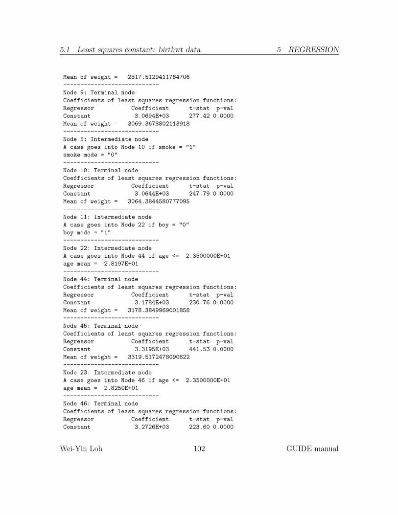
5.1 Least squares constant: birthwt data 5 REGRESSION
Mean of weight = 2817.5129411764706
----------------------------
Node 9: Terminal node
Coefficients of least squares regression functions:
Regressor Coefficient t-stat p-val
Constant 3.0694E+03 277.42 0.0000
Mean of weight = 3069.3678802113918
----------------------------
Node 5: Intermediate node
A case goes into Node 10 if smoke = "1"
smoke mode = "0"
----------------------------
Node 10: Terminal node
Coefficients of least squares regression functions:
Regressor Coefficient t-stat p-val
Constant 3.0644E+03 247.79 0.0000
Mean of weight = 3064.3844580777095
----------------------------
Node 11: Intermediate node
A case goes into Node 22 if boy = "0"
boy mode = "1"
----------------------------
Node 22: Intermediate node
A case goes into Node 44 if age <= 2.3500000E+01
age mean = 2.8197E+01
----------------------------
Node 44: Terminal node
Coefficients of least squares regression functions:
Regressor Coefficient t-stat p-val
Constant 3.1784E+03 230.76 0.0000
Mean of weight = 3178.3849969001858
----------------------------
Node 45: Terminal node
Coefficients of least squares regression functions:
Regressor Coefficient t-stat p-val
Constant 3.3195E+03 441.53 0.0000
Mean of weight = 3319.5172478090622
----------------------------
Node 23: Intermediate node
A case goes into Node 46 if age <= 2.3500000E+01
age mean = 2.8250E+01
----------------------------
Node 46: Terminal node
Coefficients of least squares regression functions:
Regressor Coefficient t-stat p-val
Constant 3.2726E+03 223.60 0.0000
Wei-Yin Loh 102 GUIDE manual
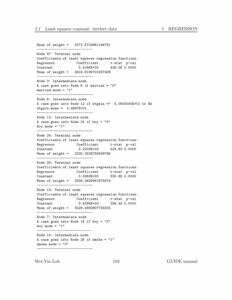
5.1 Least squares constant: birthwt data 5 REGRESSION
Mean of weight = 3272.5724861196791
----------------------------
Node 47: Terminal node
Coefficients of least squares regression functions:
Regressor Coefficient t-stat p-val
Constant 3.4166E+03 426.08 0.0000
Mean of weight = 3416.6199701937408
----------------------------
Node 3: Intermediate node
A case goes into Node 6 if married = "0"
married mode = "1"
----------------------------
Node 6: Intermediate node
A case goes into Node 12 if wtgain <= 4.0500000E+01 or NA
wtgain mean = 3.9897E+01
----------------------------
Node 12: Intermediate node
A case goes into Node 24 if boy = "0"
boy mode = "1"
----------------------------
Node 24: Terminal node
Coefficients of least squares regression functions:
Regressor Coefficient t-stat p-val
Constant 3.2203E+03 329.63 0.0000
Mean of weight = 3220.2526758409786
----------------------------
Node 25: Terminal node
Coefficients of least squares regression functions:
Regressor Coefficient t-stat p-val
Constant 3.3363E+03 335.85 0.0000
Mean of weight = 3336.2626661875674
----------------------------
Node 13: Terminal node
Coefficients of least squares regression functions:
Regressor Coefficient t-stat p-val
Constant 3.4295E+03 356.49 0.0000
Mean of weight = 3429.4892807745505
----------------------------
Node 7: Intermediate node
A case goes into Node 14 if boy = "0"
boy mode = "1"
----------------------------
Node 14: Intermediate node
A case goes into Node 28 if smoke = "1"
smoke mode = "0"
----------------------------
Wei-Yin Loh 103 GUIDE manual
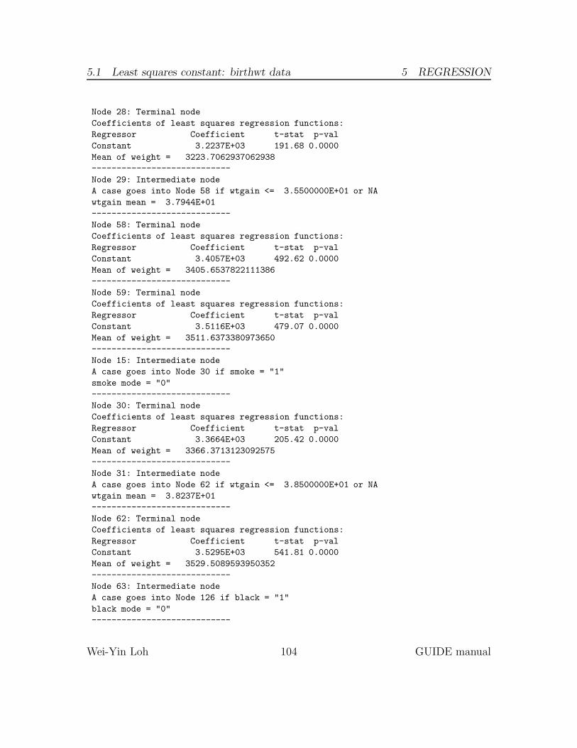
5.1 Least squares constant: birthwt data 5 REGRESSION
Node 28: Terminal node
Coefficients of least squares regression functions:
Regressor Coefficient t-stat p-val
Constant 3.2237E+03 191.68 0.0000
Mean of weight = 3223.7062937062938
----------------------------
Node 29: Intermediate node
A case goes into Node 58 if wtgain <= 3.5500000E+01 or NA
wtgain mean = 3.7944E+01
----------------------------
Node 58: Terminal node
Coefficients of least squares regression functions:
Regressor Coefficient t-stat p-val
Constant 3.4057E+03 492.62 0.0000
Mean of weight = 3405.6537822111386
----------------------------
Node 59: Terminal node
Coefficients of least squares regression functions:
Regressor Coefficient t-stat p-val
Constant 3.5116E+03 479.07 0.0000
Mean of weight = 3511.6373380973650
----------------------------
Node 15: Intermediate node
A case goes into Node 30 if smoke = "1"
smoke mode = "0"
----------------------------
Node 30: Terminal node
Coefficients of least squares regression functions:
Regressor Coefficient t-stat p-val
Constant 3.3664E+03 205.42 0.0000
Mean of weight = 3366.3713123092575
----------------------------
Node 31: Intermediate node
A case goes into Node 62 if wtgain <= 3.8500000E+01 or NA
wtgain mean = 3.8237E+01
----------------------------
Node 62: Terminal node
Coefficients of least squares regression functions:
Regressor Coefficient t-stat p-val
Constant 3.5295E+03 541.81 0.0000
Mean of weight = 3529.5089593950352
----------------------------
Node 63: Intermediate node
A case goes into Node 126 if black = "1"
black mode = "0"
----------------------------
Wei-Yin Loh 104 GUIDE manual

5.1 Least squares constant: birthwt data 5 REGRESSION
Node 126: Terminal node
Coefficients of least squares regression functions:
Regressor Coefficient t-stat p-val
Constant 3.4510E+03 111.52 0.0000
Mean of weight = 3450.9702380952381
----------------------------
Node 127: Terminal node
Coefficients of least squares regression functions:
Regressor Coefficient t-stat p-val
Constant 3.6688E+03 450.62 0.0000
Mean of weight = 3668.7919857069933
----------------------------
Proportion of variance (R-squared) explained by tree model: .0910
Observed and fitted values are stored in cons.fit
LaTeX code for tree is in cons.tex
Split and fit variable names are stored in cons.var
Figure 9 shows the tree diagram. It is rather large and may not be so easyto interpret. This is because the complexity of a piecewise-constant model restscompletely in the tree structure. GUIDE has 4 options that will reduce the tree sizeby moving some of the complexity to the nodes of the tree.
Wei-Yin Loh 105 GUIDE manual
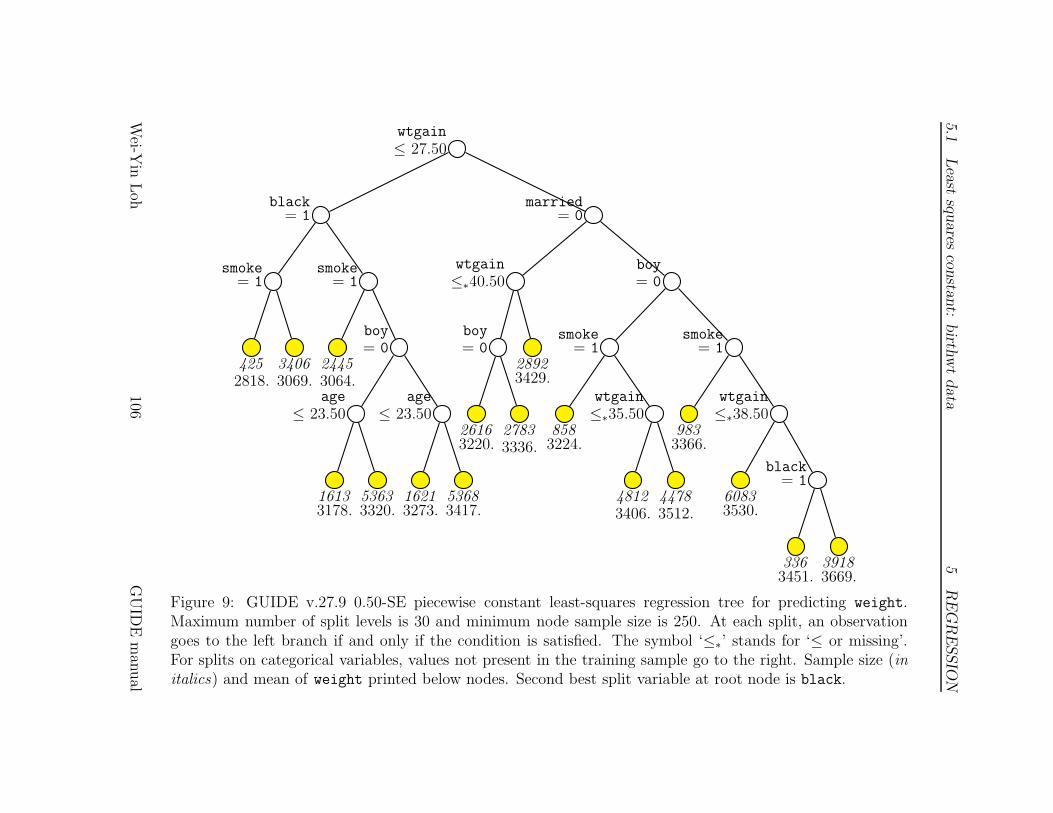
5.1
Least
squares
consta
nt:
birth
wtdata
5REGRESSIO
N
wtgain≤ 27.50
black= 1
smoke= 1
4252818.
34063069.
smoke= 1
24453064.
boy= 0
age≤ 23.50
16133178.
53633320.
age≤ 23.50
16213273.
53683417.
married= 0
wtgain≤∗40.50
boy= 0
26163220.
27833336.
28923429.
boy= 0
smoke= 1
8583224.
wtgain≤∗35.50
48123406.
44783512.
smoke= 1
9833366.
wtgain≤∗38.50
60833530.
black= 1
3363451.
39183669.
Figure 9: GUIDE v.27.9 0.50-SE piecewise constant least-squares regression tree for predicting weight.Maximum number of split levels is 30 and minimum node sample size is 250. At each split, an observationgoes to the left branch if and only if the condition is satisfied. The symbol ‘≤∗’ stands for ‘≤ or missing’.For splits on categorical variables, values not present in the training sample go to the right. Sample size (initalics) and mean of weight printed below nodes. Second best split variable at root node is black.
Wei-Y
inLoh
106GUID
Eman
ual

5.1 Least squares constant: birthwt data 5 REGRESSION
5.1.3 Contents of cons.var
Following are the contents of the text file cons.var. Column 1 gives the nodenumber, column 2 is a c, s, or t, depending on whether the split variable is C or S,or if the node is terminal. Column 3 gives the name of the split variable; if the nodeis terminal, the name is printed as NONE. Column 4 gives the name of the interactingvariable if it is present; if there is no interacting variable, the split variable nameis repeated. If a node is nonterminal, column 5 contains an integer indicating thenumber of parameter values to follow on the same line. For example, the integer is 1for node 1 and it is followed by the value 0.2750000000E+02 which is the split point.(If a split is on a categorical variable, column 5 will give the number of categoricalvalues defined by the split and subsequent columns will give those values.) If a nodeis terminal, column 5 gives the node mean of the D variable. The main purpose ofthis file is to facilitate machine extraction of the split information without parsingcons.out.
1 s wtgain wtgain 1 0.2750000000E+02
2 c black black 1 "1"
4 c smoke smoke 1 "1"
8 t NONE NONE 0.2817512941E+04
4 c smoke smoke 1 "1"
9 t boy boy 0.3069367880E+04
2 c black black 1 "1"
5 c smoke smoke 1 "1"
10 t boy boy 0.3064384458E+04
5 c smoke smoke 1 "1"
11 c boy boy 1 "0"
22 s age age 1 0.2350000000E+02
44 t age age 0.3178384997E+04
45 t age age 0.3319517248E+04
11 c boy boy 1 "0"
23 s age age 1 0.2350000000E+02
46 t married married 0.3272572486E+04
47 t married married 0.3416619970E+04
3 c married married 1 "0"
6 s wtgain wtgain 1 0.4050000000E+02
12 c boy boy 1 "0"
24 t black black 0.3220252676E+04
12 c boy boy 1 "0"
25 t black black 0.3336262666E+04
13 t black black 0.3429489281E+04
3 c married married 1 "0"
7 c boy boy 1 "0"
14 c smoke smoke 1 "1"
28 t wtgain wtgain 0.3223706294E+04
14 c smoke smoke 1 "1"
29 s wtgain wtgain 1 0.3550000000E+02
Wei-Yin Loh 107 GUIDE manual

5.2 Least squares simple linear: birthwt data 5 REGRESSION
58 t black black 0.3405653782E+04
59 t black black 0.3511637338E+04
7 c boy boy 1 "0"
15 c smoke smoke 1 "1"
30 t wtgain wtgain 0.3366371312E+04
15 c smoke smoke 1 "1"
31 s wtgain wtgain 1 0.3850000000E+02
62 t age age 0.3529508959E+04
63 c black black 1 "1"
126 t NONE NONE 0.3450970238E+04
63 c black black 1 "1"
127 t age age 0.3668791986E+04
5.2 Least squares simple linear: birthwt data
Instead of fitting a constant in each node, we can fit a simple polynomial regressionmodel of the form y = β0+β1x+β2x
2+ . . . , βkxk, where the degree of the polynomial
k is pre-specified and the best predictor variable x is chosen at each node by GUIDE.We demonstrate this with k = 1 here.
5.2.1 Input file creation
0. Read the warranty disclaimer
1. Create a GUIDE input file
Input your choice: 1
Name of batch input file: lin.in
Input 1 for model fitting, 2 for importance or DIF scoring,
3 for data conversion ([1:3], <cr>=1):
Name of batch output file: lin.out
Input 1 for single tree, 2 for ensemble ([1:2], <cr>=1):
Input 1 for classification, 2 for regression, 3 for propensity score grouping
(propensity score grouping is an experimental option)
Input your choice ([1:3], <cr>=1): 2
Choose type of regression model:
1=linear, 2=quantile, 3=Poisson, 4=proportional hazards,
5=multiresponse or itemresponse, 6=longitudinal data (with T variables).
Input choice ([1:6], <cr>=1):
Input 1 for least squares, 2 least median of squares ([1:2], <cr>=1):
Choose complexity of model to use at each node:
Choose 0 for stepwise linear regression
Choose 1 for multiple regression (recommended if R variable is present,
unless there are too many N, F or B variables when stepwise is better)
Choose 2 for best polynomial in one N or F variable + R (if present)
Wei-Yin Loh 108 GUIDE manual
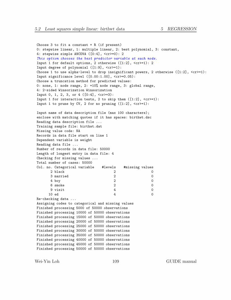
5.2 Least squares simple linear: birthwt data 5 REGRESSION
Choose 3 to fit a constant + R (if present)
0: stepwise linear, 1: multiple linear, 2: best polynomial, 3: constant,
4: stepwise simple ANCOVA ([0:4], <cr>=0): 2
This option chooses the best predictor variable at each node.
Input 1 for default options, 2 otherwise ([1:2], <cr>=1): 2
Input degree of polynomial ([1:9], <cr>=1):
Choose 1 to use alpha-level to drop insignificant powers, 2 otherwise ([1:2], <cr>=1):
Input significance level ([0.00:1.00], <cr>=0.05):
Choose a truncation method for predicted values:
0: none, 1: node range, 2: +10% node range, 3: global range,
4: 2-sided Winsorization Winsorization
Input 0, 1, 2, 3, or 4 ([0:4], <cr>=3):
Input 1 for interaction tests, 2 to skip them ([1:2], <cr>=1):
Input 1 to prune by CV, 2 for no pruning ([1:2], <cr>=1):
Input name of data description file (max 100 characters);
enclose with matching quotes if it has spaces: birthwt.dsc
Reading data description file ...
Training sample file: birthwt.dat
Missing value code: NA
Records in data file start on line 1
Dependent variable is weight
Reading data file ...
Number of records in data file: 50000
Length of longest entry in data file: 4
Checking for missing values ...
Total number of cases: 50000
Col. no. Categorical variable #levels #missing values
2 black 2 0
3 married 2 0
4 boy 2 0
6 smoke 2 0
9 visit 4 0
10 ed 4 0
Re-checking data ...
Assigning codes to categorical and missing values
Finished processing 5000 of 50000 observations
Finished processing 10000 of 50000 observations
Finished processing 15000 of 50000 observations
Finished processing 20000 of 50000 observations
Finished processing 25000 of 50000 observations
Finished processing 30000 of 50000 observations
Finished processing 35000 of 50000 observations
Finished processing 40000 of 50000 observations
Finished processing 45000 of 50000 observations
Finished processing 50000 of 50000 observations
Wei-Yin Loh 109 GUIDE manual

5.2 Least squares simple linear: birthwt data 5 REGRESSION
Data checks complete
Rereading data
Total #cases w/ #missing
#cases miss. D ord. vals #X-var #N-var #F-var #S-var #B-var #C-var
50000 0 0 1 3 0 0 0 6
No weight variable in data file
No. cases used for training: 50000
Finished reading data file
Choose how you wish to deal with missing values in training or test data:
Option 1: Fit separate models to complete and incomplete cases
Option 2: Impute missing F and N values at each node with means for regression
Option 3: Fit a piecewise constant model
Input selection: ([1:3], <cr>=2):
Default number of cross-validations: 10
Input 1 to accept the default, 2 to change it ([1:2], <cr>=1):
Best tree may be chosen based on mean or median CV estimate
Input 1 for mean-based, 2 for median-based ([1:2], <cr>=1):
Input number of SEs for pruning ([0.00:1000.00], <cr>=0.50):
Choose fraction of cases for splitting
Larger values give more splits: 0 = median split and 1 = all possible splits
Default fraction is 1.0000
Choose 1 to accept default split fraction, 2 to change it
Input 1 or 2 ([1:2], <cr>=1):
Default max. number of split levels: 30
Input 1 to accept this value, 2 to change it ([1:2], <cr>=1):
Default minimum node sample size is 2499
Input 1 to use the default value, 2 to change it ([1:2], <cr>=1):
Input 1 for LaTeX tree code, 2 to skip it ([1:2], <cr>=1):
Input file name to store LaTeX code (use .tex as suffix): lin.tex
Input 1 to include node numbers, 2 to omit them ([1:2], <cr>=1):
Input 1 to number all nodes, 2 to number leaves only ([1:2], <cr>=1):
Choose color(s) for the terminal nodes:
(1) red-yellow-green
(2) red-green-blue
(3) magenta-yellow-green
(4) yellow
(5) green
(6) magenta
(7) cyan
(8) lightgray
(9) white
Input your choice ([1:9], <cr>=1):
You can store the variables and/or values used to split and fit in a file
Choose 1 to skip this step, 2 to store split and fit variables,
3 to store split variables and their values
Input your choice ([1:3], <cr>=1): 3
Wei-Yin Loh 110 GUIDE manual
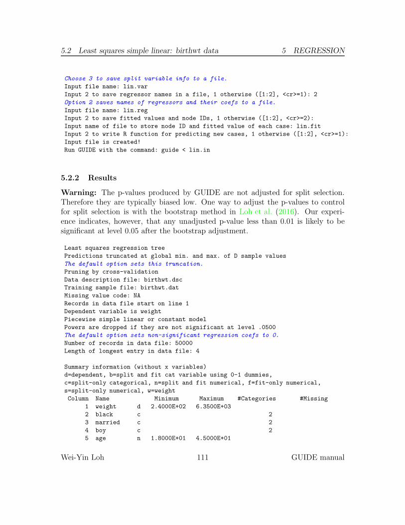
5.2 Least squares simple linear: birthwt data 5 REGRESSION
Choose 3 to save split variable info to a file.
Input file name: lin.var
Input 2 to save regressor names in a file, 1 otherwise ([1:2], <cr>=1): 2
Option 2 saves names of regressors and their coefs to a file.
Input file name: lin.reg
Input 2 to save fitted values and node IDs, 1 otherwise ([1:2], <cr>=2):
Input name of file to store node ID and fitted value of each case: lin.fit
Input 2 to write R function for predicting new cases, 1 otherwise ([1:2], <cr>=1):
Input file is created!
Run GUIDE with the command: guide < lin.in
5.2.2 Results
Warning: The p-values produced by GUIDE are not adjusted for split selection.Therefore they are typically biased low. One way to adjust the p-values to controlfor split selection is with the bootstrap method in Loh et al. (2016). Our experi-ence indicates, however, that any unadjusted p-value less than 0.01 is likely to besignificant at level 0.05 after the bootstrap adjustment.
Least squares regression tree
Predictions truncated at global min. and max. of D sample values
The default option sets this truncation.
Pruning by cross-validation
Data description file: birthwt.dsc
Training sample file: birthwt.dat
Missing value code: NA
Records in data file start on line 1
Dependent variable is weight
Piecewise simple linear or constant model
Powers are dropped if they are not significant at level .0500
The default option sets non-significant regression coefs to 0.
Number of records in data file: 50000
Length of longest entry in data file: 4
Summary information (without x variables)
d=dependent, b=split and fit cat variable using 0-1 dummies,
c=split-only categorical, n=split and fit numerical, f=fit-only numerical,
s=split-only numerical, w=weight
Column Name Minimum Maximum #Categories #Missing
1 weight d 2.4000E+02 6.3500E+03
2 black c 2
3 married c 2
4 boy c 2
5 age n 1.8000E+01 4.5000E+01
Wei-Yin Loh 111 GUIDE manual
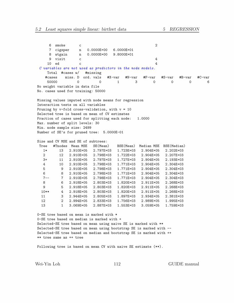
5.2 Least squares simple linear: birthwt data 5 REGRESSION
6 smoke c 2
7 cigsper n 0.0000E+00 6.0000E+01
8 wtgain n 0.0000E+00 9.8000E+01
9 visit c 4
10 ed c 4
C variables are not used as predictors in the node models.
Total #cases w/ #missing
#cases miss. D ord. vals #X-var #N-var #F-var #S-var #B-var #C-var
50000 0 0 1 3 0 0 0 6
No weight variable in data file
No. cases used for training: 50000
Missing values imputed with node means for regression
Interaction tests on all variables
Pruning by v-fold cross-validation, with v = 10
Selected tree is based on mean of CV estimates
Fraction of cases used for splitting each node: 1.0000
Max. number of split levels: 30
Min. node sample size: 2499
Number of SE’s for pruned tree: 5.0000E-01
Size and CV MSE and SE of subtrees:
Tree #Tnodes Mean MSE SE(Mean) BSE(Mean) Median MSE BSE(Median)
1* 13 2.910E+05 2.797E+03 1.723E+03 2.904E+05 2.202E+03
2 12 2.910E+05 2.798E+03 1.722E+03 2.904E+05 2.207E+03
3+ 11 2.910E+05 2.797E+03 1.727E+03 2.904E+05 2.193E+03
4 10 2.910E+05 2.798E+03 1.771E+03 2.904E+05 2.304E+03
5 9 2.910E+05 2.798E+03 1.771E+03 2.904E+05 2.304E+03
6 8 2.910E+05 2.798E+03 1.771E+03 2.904E+05 2.304E+03
7-- 7 2.910E+05 2.798E+03 1.771E+03 2.904E+05 2.304E+03
8 6 2.918E+05 2.803E+03 1.820E+03 2.911E+05 2.268E+03
9 5 2.918E+05 2.803E+03 1.820E+03 2.911E+05 2.268E+03
10** 4 2.918E+05 2.803E+03 1.820E+03 2.911E+05 2.268E+03
11 3 2.944E+05 2.805E+03 1.897E+03 2.934E+05 2.381E+03
12 2 2.994E+05 2.833E+03 1.756E+03 2.989E+05 1.995E+03
13 1 3.069E+05 2.887E+03 1.553E+03 3.059E+05 1.759E+03
0-SE tree based on mean is marked with *
0-SE tree based on median is marked with +
Selected-SE tree based on mean using naive SE is marked with **
Selected-SE tree based on mean using bootstrap SE is marked with --
Selected-SE tree based on median and bootstrap SE is marked with ++
** tree same as ++ tree
Following tree is based on mean CV with naive SE estimate (**).
Wei-Yin Loh 112 GUIDE manual

5.2 Least squares simple linear: birthwt data 5 REGRESSION
Structure of final tree. Each terminal node is marked with a T.
D-mean is mean of weight in the node
Cases fit give the number of cases used to fit node
MSE and R^2 are based on all cases in node
Node Total Cases Matrix Node Node Node Split Other
label cases fit rank D-mean MSE R^2 variable variables
1 50000 50000 2 3.371E+03 3.069E+05 0.0432 married +wtgain
2T 14369 14369 2 3.234E+03 3.166E+05 0.0558 black +wtgain
3 35631 35631 2 3.426E+03 2.925E+05 0.0394 smoke +wtgain
6T 3313 3313 2 3.198E+03 3.063E+05 0.0587 - +wtgain
7 32318 32318 2 3.449E+03 2.856E+05 0.0366 boy +wtgain
14T 15610 15610 2 3.388E+03 2.681E+05 0.0336 age +wtgain
15T 16708 16708 2 3.506E+03 2.958E+05 0.0380 age +wtgain
Number of terminal nodes of final tree: 4
Total number of nodes of final tree: 7
Second best split variable (based on curvature test) at root node is black
Regression tree:
Node 1: married = "0"
Node 2: weight-mean = 3.23443E+03
Node 1: married /= "0"
Node 3: smoke = "1"
Node 6: weight-mean = 3.19811E+03
Node 3: smoke /= "1"
Node 7: boy = "0"
Node 14: weight-mean = 3.38775E+03
Node 7: boy /= "0"
Node 15: weight-mean = 3.50636E+03
***************************************************************
WARNING: p-values below are not adjusted for split search. For a bootstrap
solution, see Loh et al. (2016), "Identification of subgroups with
differential treatment effects for longitudinal and multiresponse
variables", Statistics in Medicine, v.35, 4837-4855.
Node 1: Intermediate node
A case goes into Node 2 if married = "0"
married mode = "1"
Coefficients of least squares regression function:
Regressor Coefficient t-stat p-val Minimum Mean Maximum
Constant 3.0900E+03 482.24 0.0000
Wei-Yin Loh 113 GUIDE manual

5.2 Least squares simple linear: birthwt data 5 REGRESSION
wtgain 9.1433E+00 47.52 0.0000 0.0000E+00 3.0709E+01 9.8000E+01
Mean of weight = 3370.7566400000001
Predicted values truncated at 240.00000000000000 & 6350.0000000000000
----------------------------
Node 2: Terminal node
Coefficients of least squares regression functions:
Regressor Coefficient t-stat p-val Minimum Mean Maximum
Constant 2.9346E+03 259.41 0.0000
wtgain 9.7545E+00 29.13 0.0000 0.0000E+00 3.0737E+01 9.8000E+01
Mean of weight = 3234.4287006750642
Predicted values truncated at 240.00000000000000 & 6350.0000000000000
----------------------------
Node 3: Intermediate node
A case goes into Node 6 if smoke = "1"
smoke mode = "0"
----------------------------
Node 6: Terminal node
Coefficients of least squares regression functions:
Regressor Coefficient t-stat p-val Minimum Mean Maximum
Constant 2.9060E+03 129.19 0.0000
wtgain 9.8392E+00 14.36 0.0000 0.0000E+00 2.9688E+01 9.8000E+01
Mean of weight = 3198.1146996679745
Predicted values truncated at 240.00000000000000 & 6350.0000000000000
----------------------------
Node 7: Intermediate node
A case goes into Node 14 if boy = "0"
boy mode = "1"
----------------------------
Node 14: Terminal node
Coefficients of least squares regression functions:
Regressor Coefficient t-stat p-val Minimum Mean Maximum
Constant 3.1476E+03 283.21 0.0000
wtgain 7.8926E+00 23.29 0.0000 0.0000E+00 3.0429E+01 9.8000E+01
Mean of weight = 3387.7463164638052
Predicted values truncated at 240.00000000000000 & 6350.0000000000000
----------------------------
Node 15: Terminal node
Coefficients of least squares regression functions:
Regressor Coefficient t-stat p-val Minimum Mean Maximum
Constant 3.2296E+03 279.14 0.0000
wtgain 8.8854E+00 25.68 0.0000 0.0000E+00 3.1149E+01 9.8000E+01
Mean of weight = 3506.3593488149390
Predicted values truncated at 240.00000000000000 & 6350.0000000000000
----------------------------
Proportion of variance (R-squared) explained by tree model: .0842
Wei-Yin Loh 114 GUIDE manual
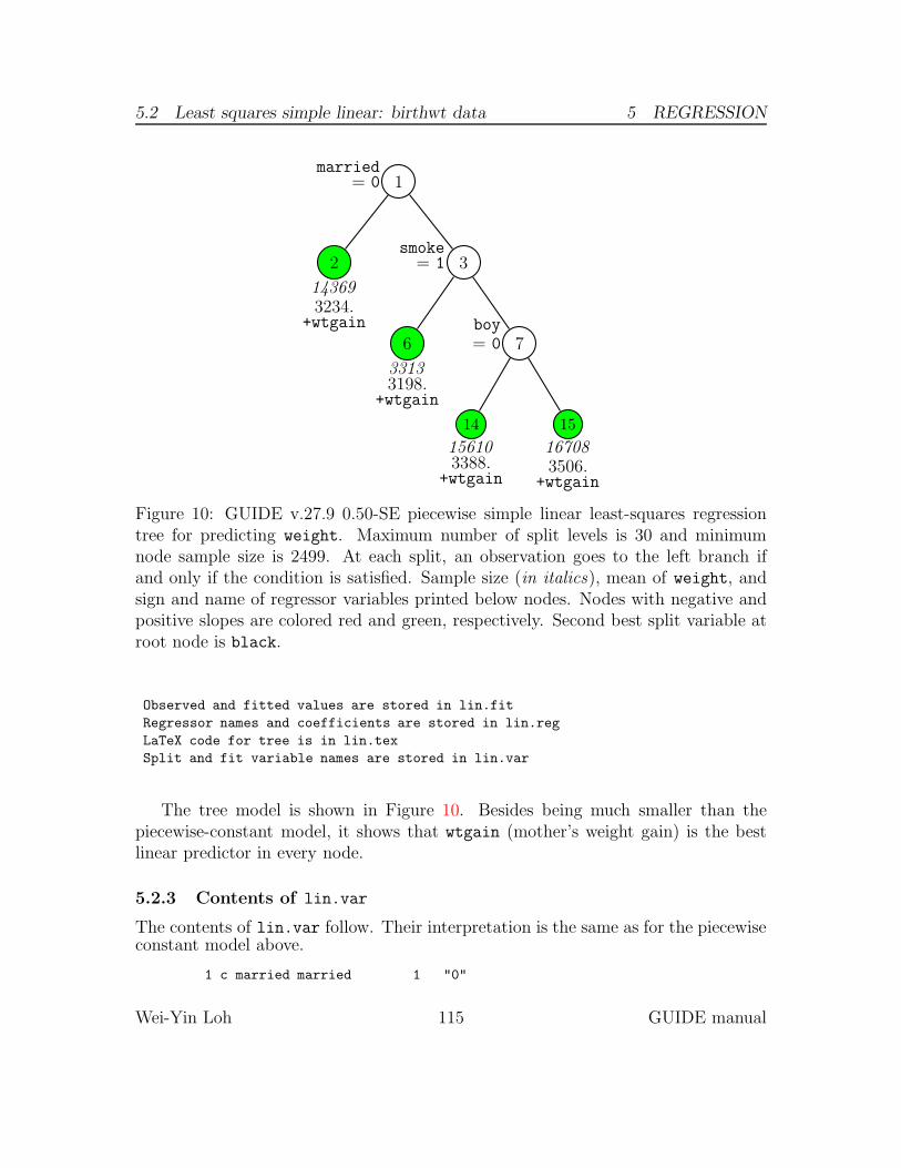
5.2 Least squares simple linear: birthwt data 5 REGRESSION
married= 0 1
2
143693234.
+wtgain
smoke= 1 3
6
33133198.
+wtgain
boy= 0 7
14
156103388.
+wtgain
15
167083506.
+wtgain
Figure 10: GUIDE v.27.9 0.50-SE piecewise simple linear least-squares regressiontree for predicting weight. Maximum number of split levels is 30 and minimumnode sample size is 2499. At each split, an observation goes to the left branch ifand only if the condition is satisfied. Sample size (in italics), mean of weight, andsign and name of regressor variables printed below nodes. Nodes with negative andpositive slopes are colored red and green, respectively. Second best split variable atroot node is black.
Observed and fitted values are stored in lin.fit
Regressor names and coefficients are stored in lin.reg
LaTeX code for tree is in lin.tex
Split and fit variable names are stored in lin.var
The tree model is shown in Figure 10. Besides being much smaller than thepiecewise-constant model, it shows that wtgain (mother’s weight gain) is the bestlinear predictor in every node.
5.2.3 Contents of lin.var
The contents of lin.var follow. Their interpretation is the same as for the piecewiseconstant model above.
1 c married married 1 "0"
Wei-Yin Loh 115 GUIDE manual
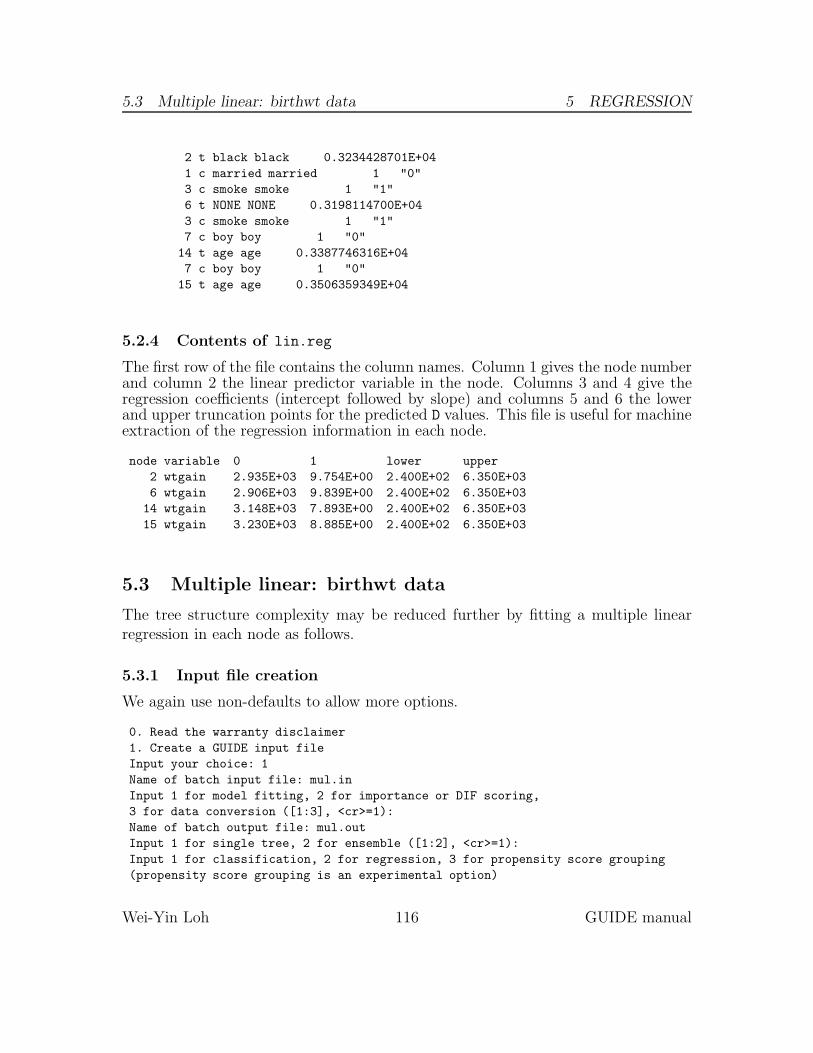
5.3 Multiple linear: birthwt data 5 REGRESSION
2 t black black 0.3234428701E+04
1 c married married 1 "0"
3 c smoke smoke 1 "1"
6 t NONE NONE 0.3198114700E+04
3 c smoke smoke 1 "1"
7 c boy boy 1 "0"
14 t age age 0.3387746316E+04
7 c boy boy 1 "0"
15 t age age 0.3506359349E+04
5.2.4 Contents of lin.reg
The first row of the file contains the column names. Column 1 gives the node numberand column 2 the linear predictor variable in the node. Columns 3 and 4 give theregression coefficients (intercept followed by slope) and columns 5 and 6 the lowerand upper truncation points for the predicted D values. This file is useful for machineextraction of the regression information in each node.
node variable 0 1 lower upper
2 wtgain 2.935E+03 9.754E+00 2.400E+02 6.350E+03
6 wtgain 2.906E+03 9.839E+00 2.400E+02 6.350E+03
14 wtgain 3.148E+03 7.893E+00 2.400E+02 6.350E+03
15 wtgain 3.230E+03 8.885E+00 2.400E+02 6.350E+03
5.3 Multiple linear: birthwt data
The tree structure complexity may be reduced further by fitting a multiple linearregression in each node as follows.
5.3.1 Input file creation
We again use non-defaults to allow more options.
0. Read the warranty disclaimer
1. Create a GUIDE input file
Input your choice: 1
Name of batch input file: mul.in
Input 1 for model fitting, 2 for importance or DIF scoring,
3 for data conversion ([1:3], <cr>=1):
Name of batch output file: mul.out
Input 1 for single tree, 2 for ensemble ([1:2], <cr>=1):
Input 1 for classification, 2 for regression, 3 for propensity score grouping
(propensity score grouping is an experimental option)
Wei-Yin Loh 116 GUIDE manual

5.3 Multiple linear: birthwt data 5 REGRESSION
Input your choice ([1:3], <cr>=1): 2
Choose type of regression model:
1=linear, 2=quantile, 3=Poisson, 4=proportional hazards,
5=multiresponse or itemresponse, 6=longitudinal data (with T variables).
Input choice ([1:6], <cr>=1):
Input 1 for least squares, 2 least median of squares ([1:2], <cr>=1):
Choose complexity of model to use at each node:
Choose 0 for stepwise linear regression
Choose 1 for multiple regression (recommended if R variable is present,
unless there are too many N, F or B variables when stepwise is better)
Choose 2 for best polynomial in one N or F variable + R (if present)
Choose 3 to fit a constant + R (if present)
0: stepwise linear, 1: multiple linear, 2: best polynomial, 3: constant,
4: stepwise simple ANCOVA ([0:4], <cr>=0): 1
Input 1 for default options, 2 otherwise ([1:2], <cr>=1): 2
More options are opened by selecting 2.
Input 2 for no intercept term, 1 otherwise ([1:2], <cr>=1):
Choose a truncation method for predicted values:
0: none, 1: node range, 2: +10% node range, 3: global range
Input 0, 1, 2, or 3 ([0:3], <cr>=3):
Input 1 for interaction tests, 2 to skip them ([1:2], <cr>=1):
Input 1 to prune by CV, 2 for no pruning ([1:2], <cr>=1):
Input name of data description file (max 100 characters);
enclose with matching quotes if it has spaces: birthwt.dsc
Reading data description file ...
Training sample file: birthwt.dat
Missing value code: NA
Records in data file start on line 1
Dependent variable is weight
Reading data file ...
Number of records in data file: 50000
Length of longest entry in data file: 4
Checking for missing values ...
Total number of cases: 50000
Col. no. Categorical variable #levels #missing values
2 black 2 0
3 married 2 0
4 boy 2 0
6 smoke 2 0
9 visit 4 0
10 ed 4 0
Re-checking data ...
Assigning codes to categorical and missing values
Finished processing 5000 of 50000 observations
Finished processing 10000 of 50000 observations
Wei-Yin Loh 117 GUIDE manual
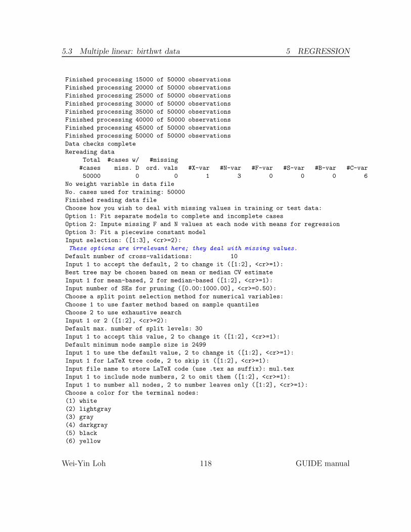
5.3 Multiple linear: birthwt data 5 REGRESSION
Finished processing 15000 of 50000 observations
Finished processing 20000 of 50000 observations
Finished processing 25000 of 50000 observations
Finished processing 30000 of 50000 observations
Finished processing 35000 of 50000 observations
Finished processing 40000 of 50000 observations
Finished processing 45000 of 50000 observations
Finished processing 50000 of 50000 observations
Data checks complete
Rereading data
Total #cases w/ #missing
#cases miss. D ord. vals #X-var #N-var #F-var #S-var #B-var #C-var
50000 0 0 1 3 0 0 0 6
No weight variable in data file
No. cases used for training: 50000
Finished reading data file
Choose how you wish to deal with missing values in training or test data:
Option 1: Fit separate models to complete and incomplete cases
Option 2: Impute missing F and N values at each node with means for regression
Option 3: Fit a piecewise constant model
Input selection: ([1:3], <cr>=2):
These options are irrelevant here; they deal with missing values.
Default number of cross-validations: 10
Input 1 to accept the default, 2 to change it ([1:2], <cr>=1):
Best tree may be chosen based on mean or median CV estimate
Input 1 for mean-based, 2 for median-based ([1:2], <cr>=1):
Input number of SEs for pruning ([0.00:1000.00], <cr>=0.50):
Choose a split point selection method for numerical variables:
Choose 1 to use faster method based on sample quantiles
Choose 2 to use exhaustive search
Input 1 or 2 ([1:2], <cr>=2):
Default max. number of split levels: 30
Input 1 to accept this value, 2 to change it ([1:2], <cr>=1):
Default minimum node sample size is 2499
Input 1 to use the default value, 2 to change it ([1:2], <cr>=1):
Input 1 for LaTeX tree code, 2 to skip it ([1:2], <cr>=1):
Input file name to store LaTeX code (use .tex as suffix): mul.tex
Input 1 to include node numbers, 2 to omit them ([1:2], <cr>=1):
Input 1 to number all nodes, 2 to number leaves only ([1:2], <cr>=1):
Choose a color for the terminal nodes:
(1) white
(2) lightgray
(3) gray
(4) darkgray
(5) black
(6) yellow
Wei-Yin Loh 118 GUIDE manual

5.3 Multiple linear: birthwt data 5 REGRESSION
(7) red
(8) blue
(9) green
(10) magenta
(11) cyan
Input your choice ([1:11], <cr>=6):
You can store the variables and/or values used to split and fit in a file
Choose 1 to skip this step, 2 to store split and fit variables,
3 to store split variables and their values
Input your choice ([1:3], <cr>=1): 3
Input file name: mul.var
Input 2 to save truncation limits and regression coefficients in a file, 1 otherwise ([1:2], <cr>=1):
Input file name: mul.reg
Input 2 to save fitted values and node IDs, 1 otherwise ([1:2], <cr>=2):
Input name of file to store node ID and fitted value of each case: mul.fit
Input 2 to write R function for predicting new cases, 1 otherwise ([1:2], <cr>=1):
Input file is created!
Run GUIDE with the command: guide < mul.in
5.3.2 Results
Least squares regression tree
Predictions truncated at global min. and max. of D sample values
Truncation of predicted values can be changed by selecting a non-default option.
Pruning by cross-validation
Data description file: birthwt.dsc
Training sample file: birthwt.dat
Missing value code: NA
Records in data file start on line 1
Dependent variable is weight
Piecewise linear model
Number of records in data file: 50000
Length of longest entry in data file: 4
Summary information (without x variables)
d=dependent, b=split and fit cat variable using 0-1 dummies,
c=split-only categorical, n=split and fit numerical, f=fit-only numerical,
s=split-only numerical, w=weight
Column Name Minimum Maximum #Categories #Missing
1 weight d 2.4000E+02 6.3500E+03
2 black c 2
3 married c 2
4 boy c 2
5 age n 1.8000E+01 4.5000E+01
6 smoke c 2
Wei-Yin Loh 119 GUIDE manual
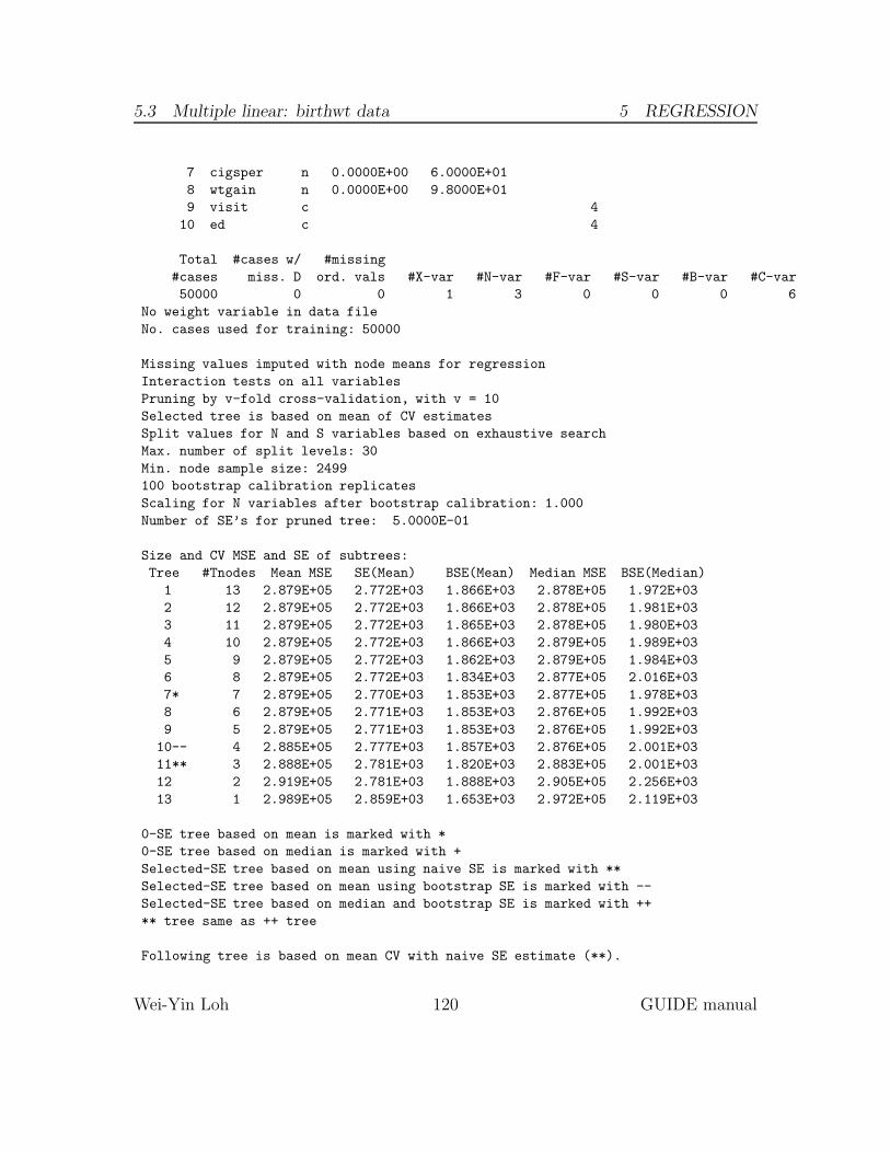
5.3 Multiple linear: birthwt data 5 REGRESSION
7 cigsper n 0.0000E+00 6.0000E+01
8 wtgain n 0.0000E+00 9.8000E+01
9 visit c 4
10 ed c 4
Total #cases w/ #missing
#cases miss. D ord. vals #X-var #N-var #F-var #S-var #B-var #C-var
50000 0 0 1 3 0 0 0 6
No weight variable in data file
No. cases used for training: 50000
Missing values imputed with node means for regression
Interaction tests on all variables
Pruning by v-fold cross-validation, with v = 10
Selected tree is based on mean of CV estimates
Split values for N and S variables based on exhaustive search
Max. number of split levels: 30
Min. node sample size: 2499
100 bootstrap calibration replicates
Scaling for N variables after bootstrap calibration: 1.000
Number of SE’s for pruned tree: 5.0000E-01
Size and CV MSE and SE of subtrees:
Tree #Tnodes Mean MSE SE(Mean) BSE(Mean) Median MSE BSE(Median)
1 13 2.879E+05 2.772E+03 1.866E+03 2.878E+05 1.972E+03
2 12 2.879E+05 2.772E+03 1.866E+03 2.878E+05 1.981E+03
3 11 2.879E+05 2.772E+03 1.865E+03 2.878E+05 1.980E+03
4 10 2.879E+05 2.772E+03 1.866E+03 2.879E+05 1.989E+03
5 9 2.879E+05 2.772E+03 1.862E+03 2.879E+05 1.984E+03
6 8 2.879E+05 2.772E+03 1.834E+03 2.877E+05 2.016E+03
7* 7 2.879E+05 2.770E+03 1.853E+03 2.877E+05 1.978E+03
8 6 2.879E+05 2.771E+03 1.853E+03 2.876E+05 1.992E+03
9 5 2.879E+05 2.771E+03 1.853E+03 2.876E+05 1.992E+03
10-- 4 2.885E+05 2.777E+03 1.857E+03 2.876E+05 2.001E+03
11** 3 2.888E+05 2.781E+03 1.820E+03 2.883E+05 2.001E+03
12 2 2.919E+05 2.781E+03 1.888E+03 2.905E+05 2.256E+03
13 1 2.989E+05 2.859E+03 1.653E+03 2.972E+05 2.119E+03
0-SE tree based on mean is marked with *
0-SE tree based on median is marked with +
Selected-SE tree based on mean using naive SE is marked with **
Selected-SE tree based on mean using bootstrap SE is marked with --
Selected-SE tree based on median and bootstrap SE is marked with ++
** tree same as ++ tree
Following tree is based on mean CV with naive SE estimate (**).
Wei-Yin Loh 120 GUIDE manual

5.3 Multiple linear: birthwt data 5 REGRESSION
Structure of final tree. Each terminal node is marked with a T.
D-mean is mean of weight in the node
Cases fit give the number of cases used to fit node
MSE and R^2 are based on all cases in node
Node Total Cases Matrix Node Node Node Split Other
label cases fit rank D-mean MSE R^2 variable variables
1 50000 50000 4 3.371E+03 2.989E+05 0.0683 black
2T 8142 8142 4 3.163E+03 3.541E+05 0.0600 boy
3 41858 41858 4 3.411E+03 2.797E+05 0.0673 boy
6T 20229 20229 4 3.352E+03 2.598E+05 0.0679 married
7T 21629 21629 4 3.467E+03 2.923E+05 0.0671 married
Number of terminal nodes of final tree: 3
Total number of nodes of final tree: 5
Second best split variable (based on curvature test) at root node is boy
Regression tree:
Node 1: black = "1"
Node 2: weight-mean = 3.16268E+03
Node 1: black /= "1"
Node 3: boy = "0"
Node 6: weight-mean = 3.35162E+03
Node 3: boy /= "0"
Node 7: weight-mean = 3.46698E+03
***************************************************************
WARNING: p-values below are not adjusted for split search. For a bootstrap
solution, see Loh et al. (2016), "Identification of subgroups with
differential treatment effects for longitudinal and multiresponse
variables", Statistics in Medicine, v.35, 4837-4855.
Node 1: Intermediate node
A case goes into Node 2 if black = "1"
black mode = "0"
Coefficients of least squares regression function:
Regressor Coefficient t-stat p-val Minimum Mean Maximum
Constant 2.8271E+03 206.14 0.0000
age 1.0226E+01 23.88 0.0000 1.8000E+01 2.7416E+01 4.5000E+01
cigsper -1.3956E+01 -26.51 0.0000 0.0000E+00 1.4766E+00 6.0000E+01
wtgain 9.2434E+00 48.57 0.0000 0.0000E+00 3.0709E+01 9.8000E+01
Mean of weight = 3370.7566400000001
Wei-Yin Loh 121 GUIDE manual

5.3 Multiple linear: birthwt data 5 REGRESSION
Predicted values truncated at 240.00000000000000 & 6350.0000000000000
----------------------------
Node 2: Terminal node
Coefficients of least squares regression functions:
Regressor Coefficient t-stat p-val Minimum Mean Maximum
Constant 2.7573E+03 82.48 0.0000
age 5.8561E+00 5.15 0.0000 1.8000E+01 2.5886E+01 4.5000E+01
cigsper -2.0286E+01 -9.79 0.0000 0.0000E+00 8.2031E-01 4.0000E+01
wtgain 9.2828E+00 19.90 0.0000 0.0000E+00 2.9133E+01 9.8000E+01
Mean of weight = 3162.6758781626136
Predicted values truncated at 240.00000000000000 & 6350.0000000000000
----------------------------
Node 3: Intermediate node
A case goes into Node 6 if boy = "0"
boy mode = "1"
----------------------------
Node 6: Terminal node
Coefficients of least squares regression functions:
Regressor Coefficient t-stat p-val Minimum Mean Maximum
Constant 2.9016E+03 140.32 0.0000
age 8.3560E+00 13.14 0.0000 1.8000E+01 2.7715E+01 4.5000E+01
cigsper -1.6363E+01 -21.80 0.0000 0.0000E+00 1.5738E+00 6.0000E+01
wtgain 7.9611E+00 27.98 0.0000 0.0000E+00 3.0667E+01 9.8000E+01
Mean of weight = 3351.6212368382025
Predicted values truncated at 240.00000000000000 & 6350.0000000000000
----------------------------
Node 7: Terminal node
Coefficients of least squares regression functions:
Regressor Coefficient t-stat p-val Minimum Mean Maximum
Constant 2.9362E+03 137.04 0.0000
age 9.5194E+00 14.55 0.0000 1.8000E+01 2.7713E+01 4.5000E+01
cigsper -1.3434E+01 -18.01 0.0000 0.0000E+00 1.6328E+00 6.0000E+01
wtgain 9.2174E+00 31.32 0.0000 0.0000E+00 3.1342E+01 9.8000E+01
Mean of weight = 3466.9831707429839
Predicted values truncated at 240.00000000000000 & 6350.0000000000000
----------------------------
Proportion of variance (R-squared) explained by tree model: .0986
Observed and fitted values are stored in mul.fit
Regressor names and coefficients are stored in mul.reg
LaTeX code for tree is in mul.tex
Split and fit variable names are stored in mul.var
Figure 11 shows the piecewise multiple linear model. Although it is slightly
Wei-Yin Loh 122 GUIDE manual

5.3 Multiple linear: birthwt data 5 REGRESSION
black= 1 1
2
81423163.
boy= 0 3
6
202293352.
7
216293467.
Figure 11: GUIDE v.27.9 0.50-SE least-squares multiple linear regression tree forpredicting weight. Maximum number of split levels is 30 and minimum node samplesize is 2499. At each split, an observation goes to the left branch if and only if thecondition is satisfied. Sample size (in italics) and mean of weight printed belownodes. Second best split variable at root node is boy.
smaller than the piecewise best simple linear model, it conveys less informationbecause the multiple linear regression coefficients in the nodes are not shown.
5.3.3 Contents of mul.var
The contents of mul.var follow.
1 c black black 1 "1"
2 t boy boy 0.3162675878E+04
1 c black black 1 "1"
3 c boy boy 1 "0"
6 t married married 0.3351621237E+04
3 c boy boy 1 "0"
7 t married married 0.3466983171E+04
5.3.4 Contents of mul.reg
The file mul.reg give the node number and the regression coefficients in each node.
Node Constant age cigsper wtgain
2 2.7573E+03 5.8561E+00 -2.0286E+01 9.2828E+00
6 2.9016E+03 8.3560E+00 -1.6363E+01 7.9611E+00
7 2.9362E+03 9.5194E+00 -1.3434E+01 9.2174E+00
Wei-Yin Loh 123 GUIDE manual

5.4 Stepwise linear: birthwt data 5 REGRESSION
5.4 Stepwise linear: birthwt data
Yet another option is to fit a stepwise linear regression model in each node. Thismay be better than the piecewise multiple liner model if it reduces the number oflinear predictors in some of the nodes.
5.4.1 Input file creation
0. Read the warranty disclaimer
1. Create a GUIDE input file
Input your choice: 1
Name of batch input file: step.in
Input 1 for model fitting, 2 for importance or DIF scoring,
3 for data conversion ([1:3], <cr>=1):
Name of batch output file: step.out
Input 1 for single tree, 2 for ensemble ([1:2], <cr>=1):
Input 1 for classification, 2 for regression, 3 for propensity score grouping
(propensity score grouping is an experimental option)
Input your choice ([1:3], <cr>=1): 2
Choose type of regression model:
1=linear, 2=quantile, 3=Poisson, 4=proportional hazards,
5=multiresponse or itemresponse, 6=longitudinal data (with T variables).
Input choice ([1:6], <cr>=1):
Input 1 for least squares, 2 least median of squares ([1:2], <cr>=1):
Choose complexity of model to use at each node:
Choose 0 for stepwise linear regression
Choose 1 for multiple regression (recommended if R variable is present,
unless there are too many N, F or B variables when stepwise is better)
Choose 2 for best polynomial in one N or F variable + R (if present)
Choose 3 to fit a constant + R (if present)
0: stepwise linear, 1: multiple linear, 2: best polynomial, 3: constant,
4: stepwise simple ANCOVA ([0:4], <cr>=0):
Input 1 for default options, 2 otherwise ([1:2], <cr>=1):
Input name of data description file (max 100 characters);
enclose with matching quotes if it has spaces: birthwt.dsc
Reading data description file ...
Training sample file: birthwt.dat
Missing value code: NA
Records in data file start on line 1
Dependent variable is weight
Reading data file ...
Number of records in data file: 50000
Length of longest entry in data file: 4
Checking for missing values ...
Wei-Yin Loh 124 GUIDE manual

5.4 Stepwise linear: birthwt data 5 REGRESSION
Total number of cases: 50000
Col. no. Categorical variable #levels #missing values
2 black 2 0
3 married 2 0
4 boy 2 0
6 smoke 2 0
9 visit 4 0
10 ed 4 0
Re-checking data ...
Assigning codes to categorical and missing values
Finished processing 5000 of 50000 observations
Finished processing 10000 of 50000 observations
Finished processing 15000 of 50000 observations
Finished processing 20000 of 50000 observations
Finished processing 25000 of 50000 observations
Finished processing 30000 of 50000 observations
Finished processing 35000 of 50000 observations
Finished processing 40000 of 50000 observations
Finished processing 45000 of 50000 observations
Finished processing 50000 of 50000 observations
Data checks complete
Rereading data
Total #cases w/ #missing
#cases miss. D ord. vals #X-var #N-var #F-var #S-var #B-var #C-var
50000 0 0 1 3 0 0 0 6
No weight variable in data file
No. cases used for training: 50000
Finished reading data file
Input 1 for LaTeX tree code, 2 to skip it ([1:2], <cr>=1):
Input file name to store LaTeX code (use .tex as suffix): step.tex
Input 2 to save fitted values and node IDs, 1 otherwise ([1:2], <cr>=2):
Input name of file to store node ID and fitted value of each case: step.fit
Input 2 to write R function for predicting new cases, 1 otherwise ([1:2], <cr>=1):
Input file is created!
Run GUIDE with the command: guide < step.in
The result is the same as that for the multiple linear regression option in thisexample.
5.4.2 Contents of step.reg
The contents of step.reg are slightly different from that of mul.reg. Instead ofgiving the estimated regression coefficients in each node, it gives the names of thevariables selected to fit each node. The node number is given in column 1 and thelower and upper truncation limits in columns 2 and 3.
Wei-Yin Loh 125 GUIDE manual

5.5 Best ANCOVA: birthwt data 5 REGRESSION
node lower upper variables
2 2.400E+02 6.350E+03 age cigsper wtgain
6 2.400E+02 6.350E+03 age cigsper wtgain
7 2.400E+02 6.350E+03 age cigsper wtgain
5.5 Best ANCOVA: birthwt data
In the best simple polynomial model, categorical variables that are specified as Care used only to split the nodes. Sometimes, it may be desired to let them alsoserve as linear predictors by means of their dummy variables. This can be done inthe multiple linear and stepwise linear options by simply specifying the categoricalvariables as B instead of C. The same can also be done in the best simple polynomialmodel, but this has the undesirable effect that a single dummy variable may bechosen as the best linear predictor in a node. A better alternative is the best simpleANCOVA option, where at each node, (i) a single N or F variable is selected as thebest linear predictor and (ii) stepwise regression is used to select a subset of thedummy variables as additional predictors. We demonstrate this by first editing thedescription file so that C variables are changed to B as follows. The resulting file isnamed birthwtancova.dsc.
birthwt.dat
NA
1
1 weight d
2 black b
3 married b
4 boy b
5 age n
6 smoke b
7 cigsper n
8 wtgain n
9 visit b
10 ed b
11 lowbwt x
5.5.1 Input file creation
0. Read the warranty disclaimer
1. Create a GUIDE input file
Input your choice: 1
Name of batch input file: ancova.in
Input 1 for model fitting, 2 for importance or DIF scoring,
3 for data conversion ([1:3], <cr>=1):
Name of batch output file: ancova.out
Wei-Yin Loh 126 GUIDE manual

5.5 Best ANCOVA: birthwt data 5 REGRESSION
Input 1 for single tree, 2 for ensemble ([1:2], <cr>=1):
Input 1 for classification, 2 for regression, 3 for propensity score grouping
(propensity score grouping is an experimental option)
Input your choice ([1:3], <cr>=1): 2
Choose type of regression model:
1=linear, 2=quantile, 3=Poisson, 4=proportional hazards,
5=multiresponse or itemresponse, 6=longitudinal data (with T variables).
Input choice ([1:6], <cr>=1):
Input 1 for least squares, 2 least median of squares ([1:2], <cr>=1):
Choose complexity of model to use at each node:
Choose 0 for stepwise linear regression
Choose 1 for multiple regression (recommended if R variable is present,
unless there are too many N, F or B variables when stepwise is better)
Choose 2 for best polynomial in one N or F variable + R (if present)
Choose 3 to fit a constant + R (if present)
0: stepwise linear, 1: multiple linear, 2: best polynomial, 3: constant,
4: stepwise simple ANCOVA ([0:4], <cr>=0): 4
This is where the ANCOVA option is selected.
Input 1 for default options, 2 otherwise ([1:2], <cr>=1):2
Input 1 for default options, 2 otherwise ([1:2], <cr>=1): 2
Input the maximum number of variables to be selected
0 indicates that the largest possible value is used
Input maximum number of variables to be selected ([0:], <cr>=0):
Input F-to-enter value ([0.01:], <cr>=4.00):
Input F-to-delete value ([0.01:], <cr>=3.99):
Choose a truncation method for predicted values:
0: none, 1: node range, 2: +10% node range, 3: global range,
4: 2-sided Winsorization Winsorization
Input 0, 1, 2, 3, or 4 ([0:4], <cr>=3):
Input 1 for interaction tests, 2 to skip them ([1:2], <cr>=1):
Input 1 to prune by CV, 2 for no pruning ([1:2], <cr>=1):
Input name of data description file (max 100 characters);
enclose with matching quotes if it has spaces: birthwtancova.dsc
Reading data description file ...
Training sample file: birthwt.dat
Missing value code: NA
Records in data file start on line 1
Dependent variable is weight
Reading data file ...
Number of records in data file: 50000
Length of longest entry in data file: 4
Checking for missing values ...
Total number of cases: 50000
Col. no. Categorical variable #levels #missing values
2 black 2 0
Wei-Yin Loh 127 GUIDE manual
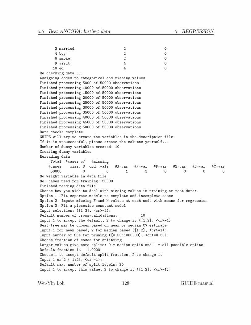
5.5 Best ANCOVA: birthwt data 5 REGRESSION
3 married 2 0
4 boy 2 0
6 smoke 2 0
9 visit 4 0
10 ed 4 0
Re-checking data ...
Assigning codes to categorical and missing values
Finished processing 5000 of 50000 observations
Finished processing 10000 of 50000 observations
Finished processing 15000 of 50000 observations
Finished processing 20000 of 50000 observations
Finished processing 25000 of 50000 observations
Finished processing 30000 of 50000 observations
Finished processing 35000 of 50000 observations
Finished processing 40000 of 50000 observations
Finished processing 45000 of 50000 observations
Finished processing 50000 of 50000 observations
Data checks complete
GUIDE will try to create the variables in the description file.
If it is unsuccessful, please create the columns yourself...
Number of dummy variables created: 10
Creating dummy variables
Rereading data
Total #cases w/ #missing
#cases miss. D ord. vals #X-var #N-var #F-var #S-var #B-var #C-var
50000 0 0 1 3 0 0 6 0
No weight variable in data file
No. cases used for training: 50000
Finished reading data file
Choose how you wish to deal with missing values in training or test data:
Option 1: Fit separate models to complete and incomplete cases
Option 2: Impute missing F and N values at each node with means for regression
Option 3: Fit a piecewise constant model
Input selection: ([1:3], <cr>=2):
Default number of cross-validations: 10
Input 1 to accept the default, 2 to change it ([1:2], <cr>=1):
Best tree may be chosen based on mean or median CV estimate
Input 1 for mean-based, 2 for median-based ([1:2], <cr>=1):
Input number of SEs for pruning ([0.00:1000.00], <cr>=0.50):
Choose fraction of cases for splitting
Larger values give more splits: 0 = median split and 1 = all possible splits
Default fraction is 1.0000
Choose 1 to accept default split fraction, 2 to change it
Input 1 or 2 ([1:2], <cr>=1):
Default max. number of split levels: 30
Input 1 to accept this value, 2 to change it ([1:2], <cr>=1):
Wei-Yin Loh 128 GUIDE manual
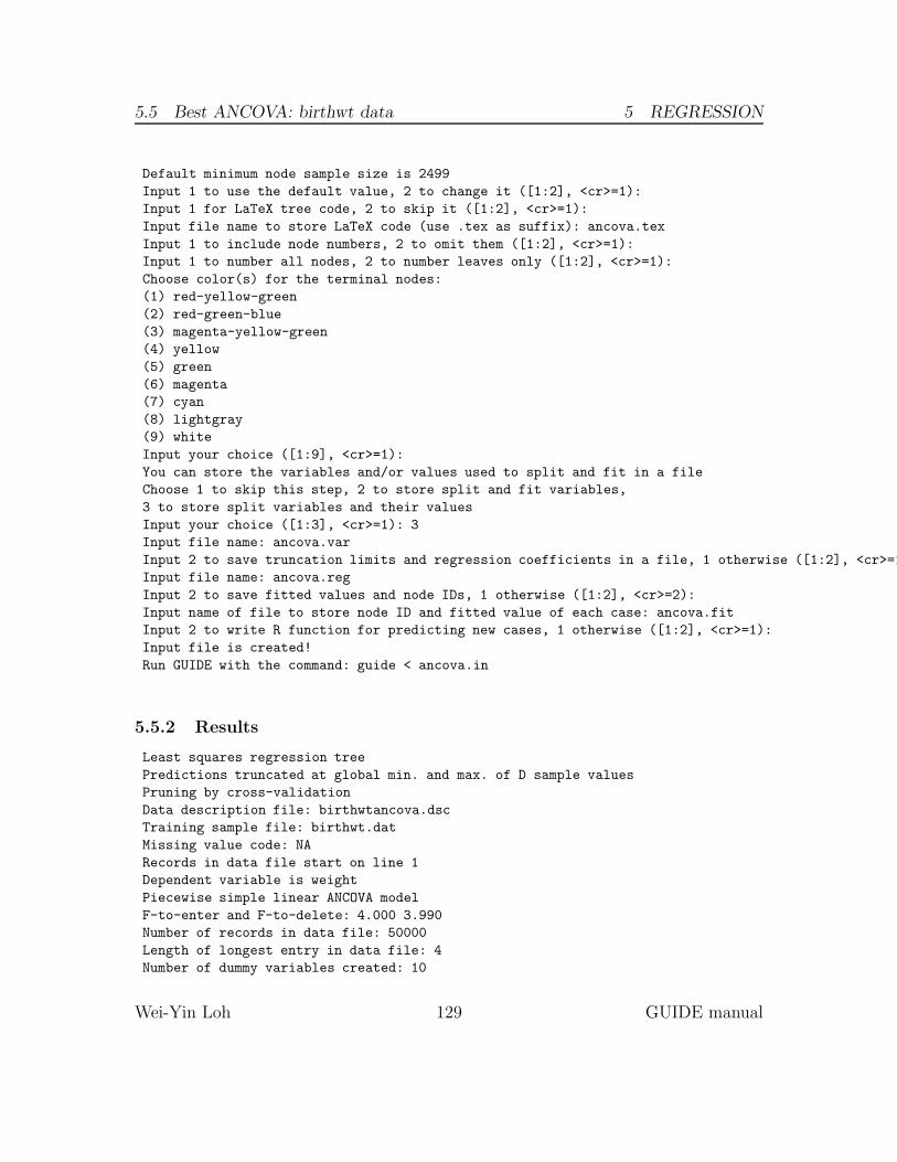
5.5 Best ANCOVA: birthwt data 5 REGRESSION
Default minimum node sample size is 2499
Input 1 to use the default value, 2 to change it ([1:2], <cr>=1):
Input 1 for LaTeX tree code, 2 to skip it ([1:2], <cr>=1):
Input file name to store LaTeX code (use .tex as suffix): ancova.tex
Input 1 to include node numbers, 2 to omit them ([1:2], <cr>=1):
Input 1 to number all nodes, 2 to number leaves only ([1:2], <cr>=1):
Choose color(s) for the terminal nodes:
(1) red-yellow-green
(2) red-green-blue
(3) magenta-yellow-green
(4) yellow
(5) green
(6) magenta
(7) cyan
(8) lightgray
(9) white
Input your choice ([1:9], <cr>=1):
You can store the variables and/or values used to split and fit in a file
Choose 1 to skip this step, 2 to store split and fit variables,
3 to store split variables and their values
Input your choice ([1:3], <cr>=1): 3
Input file name: ancova.var
Input 2 to save truncation limits and regression coefficients in a file, 1 otherwise ([1:2], <cr>=1):
Input file name: ancova.reg
Input 2 to save fitted values and node IDs, 1 otherwise ([1:2], <cr>=2):
Input name of file to store node ID and fitted value of each case: ancova.fit
Input 2 to write R function for predicting new cases, 1 otherwise ([1:2], <cr>=1):
Input file is created!
Run GUIDE with the command: guide < ancova.in
5.5.2 Results
Least squares regression tree
Predictions truncated at global min. and max. of D sample values
Pruning by cross-validation
Data description file: birthwtancova.dsc
Training sample file: birthwt.dat
Missing value code: NA
Records in data file start on line 1
Dependent variable is weight
Piecewise simple linear ANCOVA model
F-to-enter and F-to-delete: 4.000 3.990
Number of records in data file: 50000
Length of longest entry in data file: 4
Number of dummy variables created: 10
Wei-Yin Loh 129 GUIDE manual
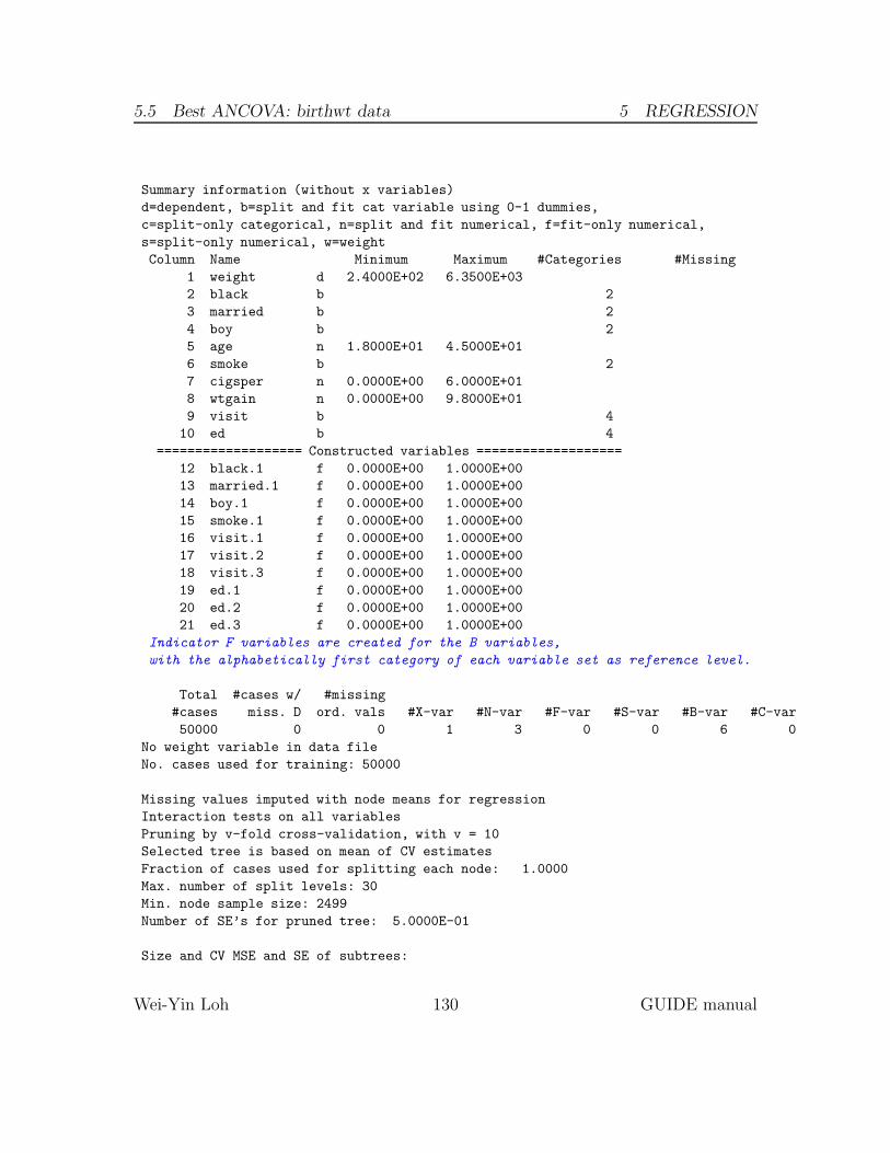
5.5 Best ANCOVA: birthwt data 5 REGRESSION
Summary information (without x variables)
d=dependent, b=split and fit cat variable using 0-1 dummies,
c=split-only categorical, n=split and fit numerical, f=fit-only numerical,
s=split-only numerical, w=weight
Column Name Minimum Maximum #Categories #Missing
1 weight d 2.4000E+02 6.3500E+03
2 black b 2
3 married b 2
4 boy b 2
5 age n 1.8000E+01 4.5000E+01
6 smoke b 2
7 cigsper n 0.0000E+00 6.0000E+01
8 wtgain n 0.0000E+00 9.8000E+01
9 visit b 4
10 ed b 4
=================== Constructed variables ===================
12 black.1 f 0.0000E+00 1.0000E+00
13 married.1 f 0.0000E+00 1.0000E+00
14 boy.1 f 0.0000E+00 1.0000E+00
15 smoke.1 f 0.0000E+00 1.0000E+00
16 visit.1 f 0.0000E+00 1.0000E+00
17 visit.2 f 0.0000E+00 1.0000E+00
18 visit.3 f 0.0000E+00 1.0000E+00
19 ed.1 f 0.0000E+00 1.0000E+00
20 ed.2 f 0.0000E+00 1.0000E+00
21 ed.3 f 0.0000E+00 1.0000E+00
Indicator F variables are created for the B variables,
with the alphabetically first category of each variable set as reference level.
Total #cases w/ #missing
#cases miss. D ord. vals #X-var #N-var #F-var #S-var #B-var #C-var
50000 0 0 1 3 0 0 6 0
No weight variable in data file
No. cases used for training: 50000
Missing values imputed with node means for regression
Interaction tests on all variables
Pruning by v-fold cross-validation, with v = 10
Selected tree is based on mean of CV estimates
Fraction of cases used for splitting each node: 1.0000
Max. number of split levels: 30
Min. node sample size: 2499
Number of SE’s for pruned tree: 5.0000E-01
Size and CV MSE and SE of subtrees:
Wei-Yin Loh 130 GUIDE manual

5.5 Best ANCOVA: birthwt data 5 REGRESSION
Tree #Tnodes Mean MSE SE(Mean) BSE(Mean) Median MSE BSE(Median)
1 14 2.869E+05 2.778E+03 1.777E+03 2.853E+05 2.154E+03
2 13 2.869E+05 2.778E+03 1.777E+03 2.853E+05 2.154E+03
3 12 2.869E+05 2.778E+03 1.789E+03 2.852E+05 2.157E+03
4 11 2.867E+05 2.774E+03 1.793E+03 2.851E+05 2.173E+03
5 10 2.867E+05 2.774E+03 1.797E+03 2.851E+05 2.158E+03
6 9 2.866E+05 2.773E+03 1.772E+03 2.851E+05 2.150E+03
7+ 8 2.866E+05 2.772E+03 1.781E+03 2.850E+05 2.157E+03
8 7 2.866E+05 2.771E+03 1.823E+03 2.851E+05 1.942E+03
9 5 2.867E+05 2.769E+03 1.871E+03 2.852E+05 2.031E+03
10 4 2.866E+05 2.768E+03 1.909E+03 2.852E+05 2.032E+03
11++ 3 2.865E+05 2.765E+03 1.838E+03 2.855E+05 2.045E+03
12 2 2.867E+05 2.763E+03 1.936E+03 2.861E+05 2.370E+03
13** 1 2.873E+05 2.766E+03 1.904E+03 2.868E+05 2.273E+03
0-SE tree based on mean is marked with *
0-SE tree based on median is marked with +
Selected-SE tree based on mean using naive SE is marked with **
Selected-SE tree based on mean using bootstrap SE is marked with --
Selected-SE tree based on median and bootstrap SE is marked with ++
** tree same as -- tree
* tree same as ++ tree
Following tree is based on mean CV with naive SE estimate (**).
Structure of final tree. Each terminal node is marked with a T.
D-mean is mean of weight in the node
Cases fit give the number of cases used to fit node
MSE and R^2 are based on all cases in node
Node Total Cases Matrix Node Node Node Split Other
label cases fit rank D-mean MSE R^2 variable variables
1T 50000 50000 9 3.371E+03 2.873E+05 0.1047 age +wtgain
Best split at root node is on age at 20.500000000000000
Number of terminal nodes of final tree: 1
Total number of nodes of final tree: 1
Second best split variable (based on curvature test) at root node is wtgain
Regression tree:
Node 1: weight-mean = 3.37076E+03
***************************************************************
Node 1: Terminal node
Wei-Yin Loh 131 GUIDE manual
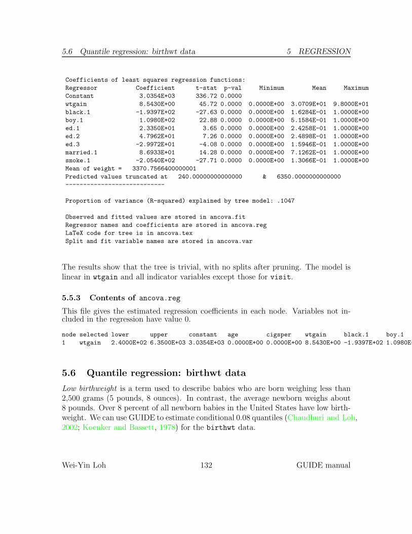
5.6 Quantile regression: birthwt data 5 REGRESSION
Coefficients of least squares regression functions:
Regressor Coefficient t-stat p-val Minimum Mean Maximum
Constant 3.0354E+03 336.72 0.0000
wtgain 8.5430E+00 45.72 0.0000 0.0000E+00 3.0709E+01 9.8000E+01
black.1 -1.9397E+02 -27.63 0.0000 0.0000E+00 1.6284E-01 1.0000E+00
boy.1 1.0980E+02 22.88 0.0000 0.0000E+00 5.1584E-01 1.0000E+00
ed.1 2.3350E+01 3.65 0.0000 0.0000E+00 2.4258E-01 1.0000E+00
ed.2 4.7962E+01 7.26 0.0000 0.0000E+00 2.4898E-01 1.0000E+00
ed.3 -2.9972E+01 -4.08 0.0000 0.0000E+00 1.5946E-01 1.0000E+00
married.1 8.6933E+01 14.28 0.0000 0.0000E+00 7.1262E-01 1.0000E+00
smoke.1 -2.0540E+02 -27.71 0.0000 0.0000E+00 1.3066E-01 1.0000E+00
Mean of weight = 3370.7566400000001
Predicted values truncated at 240.00000000000000 & 6350.0000000000000
----------------------------
Proportion of variance (R-squared) explained by tree model: .1047
Observed and fitted values are stored in ancova.fit
Regressor names and coefficients are stored in ancova.reg
LaTeX code for tree is in ancova.tex
Split and fit variable names are stored in ancova.var
The results show that the tree is trivial, with no splits after pruning. The model islinear in wtgain and all indicator variables except those for visit.
5.5.3 Contents of ancova.reg
This file gives the estimated regression coefficients in each node. Variables not in-cluded in the regression have value 0.
node selected lower upper constant age cigsper wtgain black.1 boy.1
1 wtgain 2.4000E+02 6.3500E+03 3.0354E+03 0.0000E+00 0.0000E+00 8.5430E+00 -1.9397E+02 1.0980E+02
5.6 Quantile regression: birthwt data
Low birthweight is a term used to describe babies who are born weighing less than2,500 grams (5 pounds, 8 ounces). In contrast, the average newborn weighs about8 pounds. Over 8 percent of all newborn babies in the United States have low birth-weight. We can use GUIDE to estimate conditional 0.08 quantiles (Chaudhuri and Loh,2002; Koenker and Bassett, 1978) for the birthwt data.
Wei-Yin Loh 132 GUIDE manual
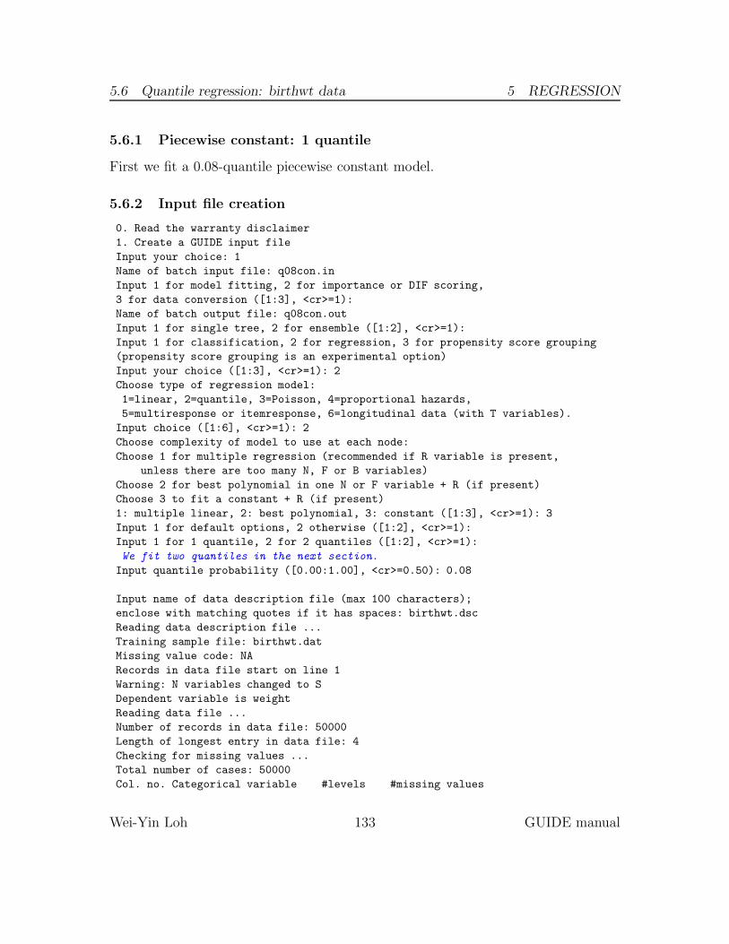
5.6 Quantile regression: birthwt data 5 REGRESSION
5.6.1 Piecewise constant: 1 quantile
First we fit a 0.08-quantile piecewise constant model.
5.6.2 Input file creation
0. Read the warranty disclaimer
1. Create a GUIDE input file
Input your choice: 1
Name of batch input file: q08con.in
Input 1 for model fitting, 2 for importance or DIF scoring,
3 for data conversion ([1:3], <cr>=1):
Name of batch output file: q08con.out
Input 1 for single tree, 2 for ensemble ([1:2], <cr>=1):
Input 1 for classification, 2 for regression, 3 for propensity score grouping
(propensity score grouping is an experimental option)
Input your choice ([1:3], <cr>=1): 2
Choose type of regression model:
1=linear, 2=quantile, 3=Poisson, 4=proportional hazards,
5=multiresponse or itemresponse, 6=longitudinal data (with T variables).
Input choice ([1:6], <cr>=1): 2
Choose complexity of model to use at each node:
Choose 1 for multiple regression (recommended if R variable is present,
unless there are too many N, F or B variables)
Choose 2 for best polynomial in one N or F variable + R (if present)
Choose 3 to fit a constant + R (if present)
1: multiple linear, 2: best polynomial, 3: constant ([1:3], <cr>=1): 3
Input 1 for default options, 2 otherwise ([1:2], <cr>=1):
Input 1 for 1 quantile, 2 for 2 quantiles ([1:2], <cr>=1):
We fit two quantiles in the next section.
Input quantile probability ([0.00:1.00], <cr>=0.50): 0.08
Input name of data description file (max 100 characters);
enclose with matching quotes if it has spaces: birthwt.dsc
Reading data description file ...
Training sample file: birthwt.dat
Missing value code: NA
Records in data file start on line 1
Warning: N variables changed to S
Dependent variable is weight
Reading data file ...
Number of records in data file: 50000
Length of longest entry in data file: 4
Checking for missing values ...
Total number of cases: 50000
Col. no. Categorical variable #levels #missing values
Wei-Yin Loh 133 GUIDE manual

5.6 Quantile regression: birthwt data 5 REGRESSION
2 black 2 0
3 married 2 0
4 boy 2 0
6 smoke 2 0
9 visit 4 0
10 ed 4 0
Re-checking data ...
Assigning codes to categorical and missing values
Finished processing 5000 of 50000 observations
Finished processing 10000 of 50000 observations
Finished processing 15000 of 50000 observations
Finished processing 20000 of 50000 observations
Finished processing 25000 of 50000 observations
Finished processing 30000 of 50000 observations
Finished processing 35000 of 50000 observations
Finished processing 40000 of 50000 observations
Finished processing 45000 of 50000 observations
Finished processing 50000 of 50000 observations
Data checks complete
Rereading data
Total #cases w/ #missing
#cases miss. D ord. vals #X-var #N-var #F-var #S-var #B-var #C-var
50000 0 0 1 0 0 3 0 6
No. cases used for training: 50000
Finished reading data file
Input 1 for LaTeX tree code, 2 to skip it ([1:2], <cr>=1):
Input file name to store LaTeX code (use .tex as suffix): q08con.tex
Input 2 to save fitted values and node IDs, 1 otherwise ([1:2], <cr>=2):
Input name of file to store node ID and fitted value of each case: q08con.fit
Input 2 to write R function for predicting new cases, 1 otherwise ([1:2], <cr>=1):
Input file is created!
Run GUIDE with the command: guide < q08con.in
5.6.3 Results
Quantile regression tree with quantile probability .0800
Pruning by cross-validation
Data description file: birthwt.dsc
Training sample file: birthwt.dat
Missing value code: NA
Records in data file start on line 1
Warning: N variables changed to S
Dependent variable is weight
Piecewise constant model
Number of records in data file: 50000
Wei-Yin Loh 134 GUIDE manual
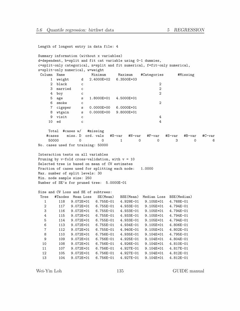
5.6 Quantile regression: birthwt data 5 REGRESSION
Length of longest entry in data file: 4
Summary information (without x variables)
d=dependent, b=split and fit cat variable using 0-1 dummies,
c=split-only categorical, n=split and fit numerical, f=fit-only numerical,
s=split-only numerical, w=weight
Column Name Minimum Maximum #Categories #Missing
1 weight d 2.4000E+02 6.3500E+03
2 black c 2
3 married c 2
4 boy c 2
5 age s 1.8000E+01 4.5000E+01
6 smoke c 2
7 cigsper s 0.0000E+00 6.0000E+01
8 wtgain s 0.0000E+00 9.8000E+01
9 visit c 4
10 ed c 4
Total #cases w/ #missing
#cases miss. D ord. vals #X-var #N-var #F-var #S-var #B-var #C-var
50000 0 0 1 0 0 3 0 6
No. cases used for training: 50000
Interaction tests on all variables
Pruning by v-fold cross-validation, with v = 10
Selected tree is based on mean of CV estimates
Fraction of cases used for splitting each node: 1.0000
Max. number of split levels: 30
Min. node sample size: 250
Number of SE’s for pruned tree: 5.0000E-01
Size and CV Loss and SE of subtrees:
Tree #Tnodes Mean Loss SE(Mean) BSE(Mean) Median Loss BSE(Median)
1 118 9.072E+01 6.755E-01 4.929E-01 9.105E+01 4.768E-01
2 117 9.072E+01 6.755E-01 4.933E-01 9.105E+01 4.794E-01
3 116 9.072E+01 6.755E-01 4.933E-01 9.105E+01 4.794E-01
4 115 9.072E+01 6.755E-01 4.933E-01 9.105E+01 4.794E-01
5 114 9.072E+01 6.755E-01 4.933E-01 9.105E+01 4.794E-01
6 113 9.072E+01 6.755E-01 4.934E-01 9.105E+01 4.806E-01
7 112 9.072E+01 6.755E-01 4.940E-01 9.105E+01 4.802E-01
8 110 9.072E+01 6.756E-01 4.935E-01 9.104E+01 4.795E-01
9 109 9.072E+01 6.756E-01 4.925E-01 9.104E+01 4.804E-01
10 108 9.072E+01 6.756E-01 4.926E-01 9.104E+01 4.810E-01
11 107 9.072E+01 6.756E-01 4.927E-01 9.104E+01 4.817E-01
12 105 9.072E+01 6.756E-01 4.927E-01 9.104E+01 4.812E-01
13 104 9.072E+01 6.756E-01 4.927E-01 9.104E+01 4.812E-01
Wei-Yin Loh 135 GUIDE manual

5.6 Quantile regression: birthwt data 5 REGRESSION
14 103 9.072E+01 6.754E-01 4.932E-01 9.104E+01 4.867E-01
15 101 9.071E+01 6.754E-01 4.927E-01 9.105E+01 4.832E-01
16 99 9.071E+01 6.754E-01 4.927E-01 9.105E+01 4.832E-01
17 98 9.072E+01 6.753E-01 4.943E-01 9.105E+01 4.880E-01
18 97 9.072E+01 6.753E-01 4.946E-01 9.105E+01 4.904E-01
19 96 9.071E+01 6.753E-01 4.951E-01 9.105E+01 4.850E-01
20 95 9.071E+01 6.753E-01 4.942E-01 9.105E+01 4.852E-01
21 94 9.071E+01 6.755E-01 4.934E-01 9.109E+01 4.701E-01
22 93 9.071E+01 6.756E-01 4.926E-01 9.109E+01 4.686E-01
23 92 9.071E+01 6.755E-01 4.925E-01 9.106E+01 4.676E-01
24 91 9.069E+01 6.755E-01 4.918E-01 9.106E+01 4.694E-01
25 89 9.069E+01 6.755E-01 4.941E-01 9.106E+01 4.696E-01
26 87 9.069E+01 6.755E-01 4.941E-01 9.106E+01 4.696E-01
27 86 9.069E+01 6.755E-01 4.941E-01 9.106E+01 4.696E-01
28 85 9.069E+01 6.755E-01 4.943E-01 9.106E+01 4.696E-01
29 84 9.069E+01 6.755E-01 4.903E-01 9.106E+01 4.681E-01
30 83 9.069E+01 6.756E-01 4.913E-01 9.106E+01 4.733E-01
31 82 9.069E+01 6.756E-01 4.911E-01 9.107E+01 4.730E-01
32 81 9.069E+01 6.756E-01 4.899E-01 9.107E+01 4.729E-01
33 80 9.069E+01 6.756E-01 4.902E-01 9.108E+01 4.755E-01
34 78 9.070E+01 6.758E-01 4.893E-01 9.108E+01 4.669E-01
35 77 9.071E+01 6.759E-01 4.882E-01 9.110E+01 4.632E-01
36 74 9.071E+01 6.759E-01 4.882E-01 9.110E+01 4.632E-01
37 73 9.071E+01 6.758E-01 4.885E-01 9.110E+01 4.656E-01
38 72 9.069E+01 6.756E-01 4.931E-01 9.110E+01 4.719E-01
39 71 9.069E+01 6.757E-01 4.967E-01 9.110E+01 4.786E-01
40 69 9.069E+01 6.758E-01 4.985E-01 9.111E+01 4.902E-01
41 68 9.066E+01 6.757E-01 4.936E-01 9.109E+01 4.802E-01
42 67 9.065E+01 6.756E-01 4.927E-01 9.104E+01 4.373E-01
43 62 9.064E+01 6.753E-01 4.902E-01 9.103E+01 4.287E-01
44 61 9.064E+01 6.753E-01 4.902E-01 9.103E+01 4.287E-01
45 60 9.064E+01 6.754E-01 4.901E-01 9.103E+01 4.321E-01
46 59 9.064E+01 6.753E-01 4.903E-01 9.103E+01 4.320E-01
47 58 9.063E+01 6.752E-01 4.899E-01 9.100E+01 4.355E-01
48 56 9.063E+01 6.752E-01 4.907E-01 9.100E+01 4.413E-01
49 55 9.062E+01 6.751E-01 4.906E-01 9.100E+01 4.440E-01
50 53 9.061E+01 6.750E-01 4.924E-01 9.095E+01 4.529E-01
51 52 9.059E+01 6.753E-01 4.947E-01 9.094E+01 4.422E-01
52 49 9.060E+01 6.754E-01 4.895E-01 9.094E+01 4.383E-01
53 48 9.056E+01 6.759E-01 4.820E-01 9.094E+01 4.540E-01
54 47 9.057E+01 6.760E-01 4.772E-01 9.094E+01 4.631E-01
55 46 9.057E+01 6.762E-01 4.772E-01 9.094E+01 4.604E-01
56 44 9.057E+01 6.761E-01 4.771E-01 9.094E+01 4.600E-01
57 43 9.058E+01 6.761E-01 4.772E-01 9.094E+01 4.581E-01
58 42 9.057E+01 6.761E-01 4.762E-01 9.092E+01 4.486E-01
59 40 9.057E+01 6.761E-01 4.762E-01 9.092E+01 4.486E-01
Wei-Yin Loh 136 GUIDE manual
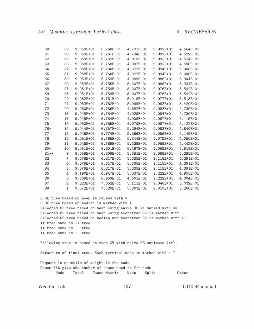
5.6 Quantile regression: birthwt data 5 REGRESSION
60 39 9.058E+01 6.760E-01 4.781E-01 9.092E+01 4.564E-01
61 38 9.059E+01 6.761E-01 4.794E-01 9.092E+01 4.522E-01
62 36 9.059E+01 6.762E-01 4.815E-01 9.092E+01 4.524E-01
63 33 9.058E+01 6.758E-01 4.807E-01 9.092E+01 4.698E-01
64 32 9.058E+01 6.760E-01 4.922E-01 9.094E+01 5.000E-01
65 31 9.058E+01 6.760E-01 4.922E-01 9.094E+01 5.000E-01
66 30 9.053E+01 6.759E-01 4.949E-01 9.086E+01 5.344E-01
67 29 9.053E+01 6.755E-01 5.007E-01 9.086E+01 5.334E-01
68 27 9.051E+01 6.754E-01 5.007E-01 9.076E+01 5.542E-01
69 25 9.051E+01 6.754E-01 5.007E-01 9.076E+01 5.542E-01
70 22 9.052E+01 6.751E-01 5.018E-01 9.077E+01 5.513E-01
71 21 9.053E+01 6.752E-01 5.069E-01 9.083E+01 5.429E-01
72 20 9.050E+01 6.756E-01 4.882E-01 9.083E+01 4.730E-01
73 18 9.048E+01 6.754E-01 4.929E-01 9.084E+01 4.730E-01
74 17 9.049E+01 6.754E-01 4.908E-01 9.087E+01 5.115E-01
75 16 9.050E+01 6.755E-01 4.970E-01 9.087E+01 5.122E-01
76* 14 9.044E+01 6.757E-01 5.294E-01 9.083E+01 4.840E-01
77 13 9.048E+01 6.774E-01 5.366E-01 9.086E+01 5.145E-01
78 12 9.051E+01 6.785E-01 5.344E-01 9.075E+01 4.050E-01
79 11 9.045E+01 6.789E-01 5.338E-01 9.068E+01 4.442E-01
80+ 10 9.051E+01 6.801E-01 5.497E-01 9.068E+01 4.918E-01
81** 9 9.058E+01 6.809E-01 5.381E-01 9.088E+01 5.385E-01
82 7 9.078E+01 6.817E-01 5.335E-01 9.118E+01 4.391E-01
83 6 9.078E+01 6.817E-01 5.335E-01 9.118E+01 4.391E-01
84 5 9.078E+01 6.817E-01 5.335E-01 9.118E+01 4.391E-01
85 4 9.190E+01 6.947E-01 5.337E-01 9.222E+01 4.955E-01
86 3 9.209E+01 6.959E-01 4.561E-01 9.222E+01 4.304E-01
87 2 9.323E+01 7.052E-01 5.111E-01 9.346E+01 5.032E-01
88 1 9.572E+01 7.520E-01 5.063E-01 9.610E+01 6.260E-01
0-SE tree based on mean is marked with *
0-SE tree based on median is marked with +
Selected-SE tree based on mean using naive SE is marked with **
Selected-SE tree based on mean using bootstrap SE is marked with --
Selected-SE tree based on median and bootstrap SE is marked with ++
** tree same as ++ tree
** tree same as -- tree
++ tree same as -- tree
Following tree is based on mean CV with naive SE estimate (**).
Structure of final tree. Each terminal node is marked with a T.
D-quant is quantile of weight in the node
Cases fit give the number of cases used to fit node
Node Total Cases Matrix Node Split Other
Wei-Yin Loh 137 GUIDE manual

5.6 Quantile regression: birthwt data 5 REGRESSION
label cases fit rank D-quant variable variables
1 50000 50000 1 2.637E+03 wtgain
2 17934 17934 1 2.438E+03 black
4 3536 3536 1 2.155E+03 wtgain
8T 1107 1107 1 1.786E+03 boy
9T 2429 2429 1 2.268E+03 smoke
5 14398 14398 1 2.523E+03 smoke
10T 2222 2222 1 2.240E+03 visit
11T 12176 12176 1 2.580E+03 married
3 32066 32066 1 2.760E+03 black
6T 4606 4606 1 2.580E+03 smoke
7 27460 27460 1 2.807E+03 smoke
14T 3519 3519 1 2.608E+03 wtgain
15 23941 23941 1 2.835E+03 married
30T 4242 4242 1 2.750E+03 visit :wtgain
31 19699 19699 1 2.863E+03 wtgain
62T 10795 10795 1 2.826E+03 ed
63T 8904 8904 1 2.925E+03 boy
Number of terminal nodes of final tree: 9
Total number of nodes of final tree: 17
Second best split variable (based on curvature test) at root node is black
Regression tree:
Node 1: wtgain <= 25.50000
Node 2: black = "1"
Node 4: wtgain <= 14.50000
Node 8: weight sample quantile = 1.78600E+03
Node 4: wtgain > 14.50000 or NA
Node 9: weight sample quantile = 2.26800E+03
Node 2: black /= "1"
Node 5: smoke = "1"
Node 10: weight sample quantile = 2.24000E+03
Node 5: smoke /= "1"
Node 11: weight sample quantile = 2.58000E+03
Node 1: wtgain > 25.50000 or NA
Node 3: black = "1"
Node 6: weight sample quantile = 2.58000E+03
Node 3: black /= "1"
Node 7: smoke = "1"
Node 14: weight sample quantile = 2.60800E+03
Node 7: smoke /= "1"
Node 15: married = "0"
Node 30: weight sample quantile = 2.75000E+03
Node 15: married /= "0"
Wei-Yin Loh 138 GUIDE manual
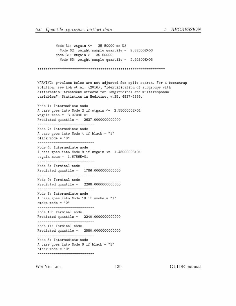
5.6 Quantile regression: birthwt data 5 REGRESSION
Node 31: wtgain <= 35.50000 or NA
Node 62: weight sample quantile = 2.82600E+03
Node 31: wtgain > 35.50000
Node 63: weight sample quantile = 2.92500E+03
***************************************************************
WARNING: p-values below are not adjusted for split search. For a bootstrap
solution, see Loh et al. (2016), "Identification of subgroups with
differential treatment effects for longitudinal and multiresponse
variables", Statistics in Medicine, v.35, 4837-4855.
Node 1: Intermediate node
A case goes into Node 2 if wtgain <= 2.5500000E+01
wtgain mean = 3.0709E+01
Predicted quantile = 2637.0000000000000
----------------------------
Node 2: Intermediate node
A case goes into Node 4 if black = "1"
black mode = "0"
----------------------------
Node 4: Intermediate node
A case goes into Node 8 if wtgain <= 1.4500000E+01
wtgain mean = 1.6786E+01
----------------------------
Node 8: Terminal node
Predicted quantile = 1786.0000000000000
----------------------------
Node 9: Terminal node
Predicted quantile = 2268.0000000000000
----------------------------
Node 5: Intermediate node
A case goes into Node 10 if smoke = "1"
smoke mode = "0"
----------------------------
Node 10: Terminal node
Predicted quantile = 2240.0000000000000
----------------------------
Node 11: Terminal node
Predicted quantile = 2580.0000000000000
----------------------------
Node 3: Intermediate node
A case goes into Node 6 if black = "1"
black mode = "0"
----------------------------
Wei-Yin Loh 139 GUIDE manual
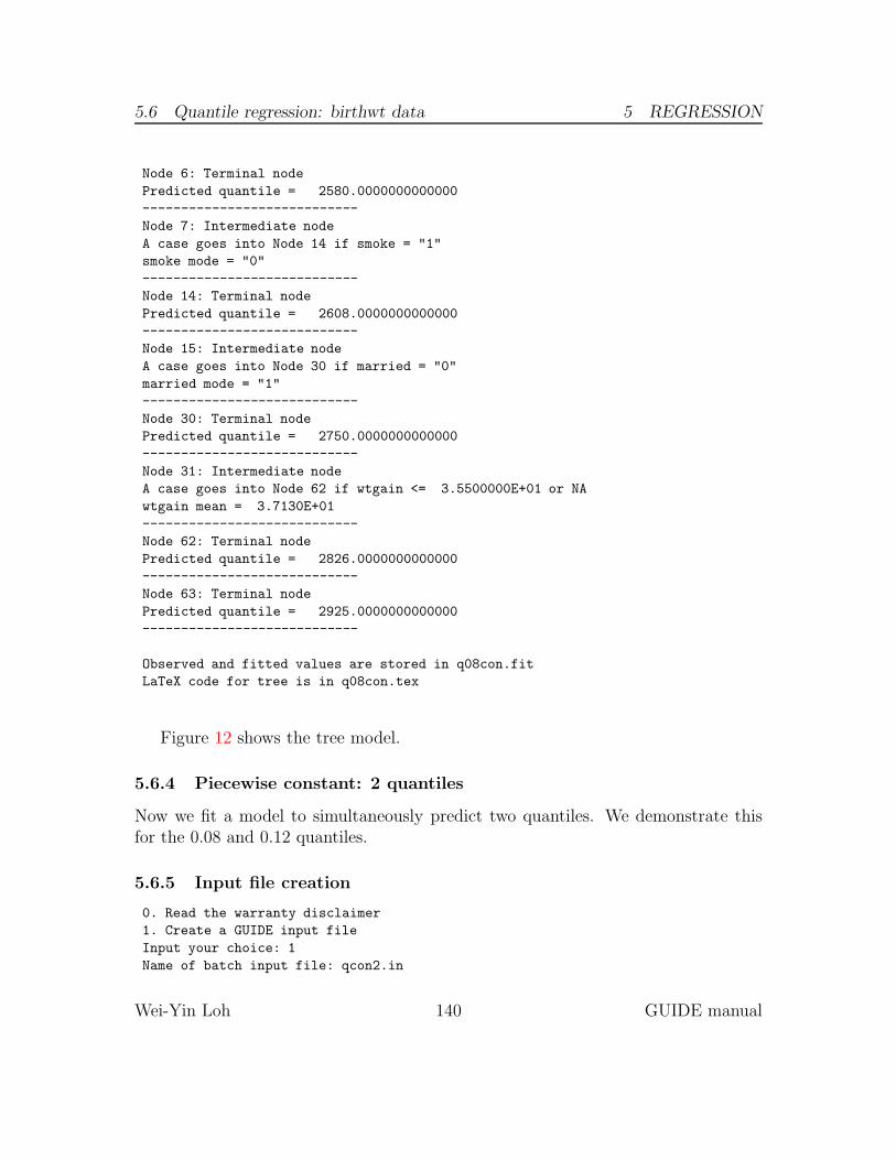
5.6 Quantile regression: birthwt data 5 REGRESSION
Node 6: Terminal node
Predicted quantile = 2580.0000000000000
----------------------------
Node 7: Intermediate node
A case goes into Node 14 if smoke = "1"
smoke mode = "0"
----------------------------
Node 14: Terminal node
Predicted quantile = 2608.0000000000000
----------------------------
Node 15: Intermediate node
A case goes into Node 30 if married = "0"
married mode = "1"
----------------------------
Node 30: Terminal node
Predicted quantile = 2750.0000000000000
----------------------------
Node 31: Intermediate node
A case goes into Node 62 if wtgain <= 3.5500000E+01 or NA
wtgain mean = 3.7130E+01
----------------------------
Node 62: Terminal node
Predicted quantile = 2826.0000000000000
----------------------------
Node 63: Terminal node
Predicted quantile = 2925.0000000000000
----------------------------
Observed and fitted values are stored in q08con.fit
LaTeX code for tree is in q08con.tex
Figure 12 shows the tree model.
5.6.4 Piecewise constant: 2 quantiles
Now we fit a model to simultaneously predict two quantiles. We demonstrate thisfor the 0.08 and 0.12 quantiles.
5.6.5 Input file creation
0. Read the warranty disclaimer
1. Create a GUIDE input file
Input your choice: 1
Name of batch input file: qcon2.in
Wei-Yin Loh 140 GUIDE manual

5.6 Quantile regression: birthwt data 5 REGRESSION
wtgain≤ 25.50 1
black= 1 2
wtgain≤ 14.50 4
8
11071786.
9
24292268.
smoke= 1 5
10
22222240.
11
121762580.
black= 1 3
6
46062580.
smoke= 1 7
14
35192608.
married= 0 15
30
42422750.
wtgain≤∗35.50 31
62
107952826.
63
89042925.
Figure 12: GUIDE v.27.9 0.50-SE piecewise constant 0.08-quantile regression treefor predicting weight. Maximum number of split levels is 30 and minimum nodesample size is 250. At each split, an observation goes to the left branch if and only ifthe condition is satisfied. The symbol ‘≤∗’ stands for ‘≤ or missing’. Sample size (initalics) and 0.08-quantiles of weight printed below nodes. Second best split variableat root node is black.
Wei-Yin Loh 141 GUIDE manual
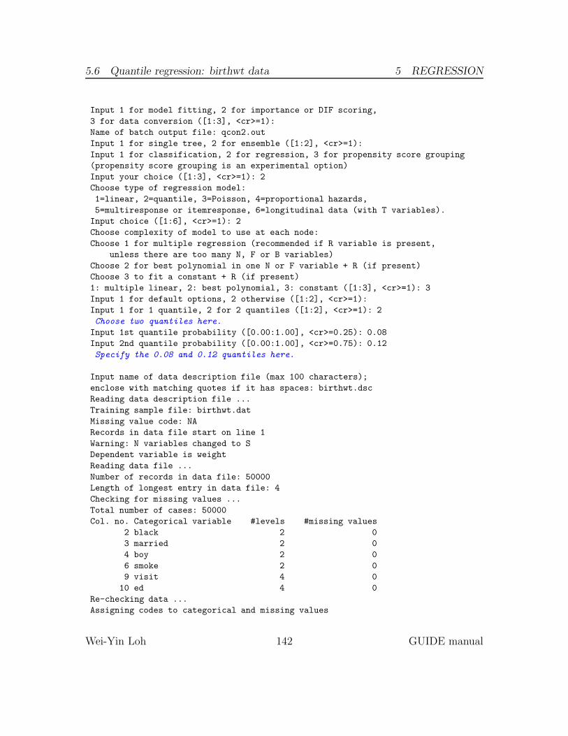
5.6 Quantile regression: birthwt data 5 REGRESSION
Input 1 for model fitting, 2 for importance or DIF scoring,
3 for data conversion ([1:3], <cr>=1):
Name of batch output file: qcon2.out
Input 1 for single tree, 2 for ensemble ([1:2], <cr>=1):
Input 1 for classification, 2 for regression, 3 for propensity score grouping
(propensity score grouping is an experimental option)
Input your choice ([1:3], <cr>=1): 2
Choose type of regression model:
1=linear, 2=quantile, 3=Poisson, 4=proportional hazards,
5=multiresponse or itemresponse, 6=longitudinal data (with T variables).
Input choice ([1:6], <cr>=1): 2
Choose complexity of model to use at each node:
Choose 1 for multiple regression (recommended if R variable is present,
unless there are too many N, F or B variables)
Choose 2 for best polynomial in one N or F variable + R (if present)
Choose 3 to fit a constant + R (if present)
1: multiple linear, 2: best polynomial, 3: constant ([1:3], <cr>=1): 3
Input 1 for default options, 2 otherwise ([1:2], <cr>=1):
Input 1 for 1 quantile, 2 for 2 quantiles ([1:2], <cr>=1): 2
Choose two quantiles here.
Input 1st quantile probability ([0.00:1.00], <cr>=0.25): 0.08
Input 2nd quantile probability ([0.00:1.00], <cr>=0.75): 0.12
Specify the 0.08 and 0.12 quantiles here.
Input name of data description file (max 100 characters);
enclose with matching quotes if it has spaces: birthwt.dsc
Reading data description file ...
Training sample file: birthwt.dat
Missing value code: NA
Records in data file start on line 1
Warning: N variables changed to S
Dependent variable is weight
Reading data file ...
Number of records in data file: 50000
Length of longest entry in data file: 4
Checking for missing values ...
Total number of cases: 50000
Col. no. Categorical variable #levels #missing values
2 black 2 0
3 married 2 0
4 boy 2 0
6 smoke 2 0
9 visit 4 0
10 ed 4 0
Re-checking data ...
Assigning codes to categorical and missing values
Wei-Yin Loh 142 GUIDE manual
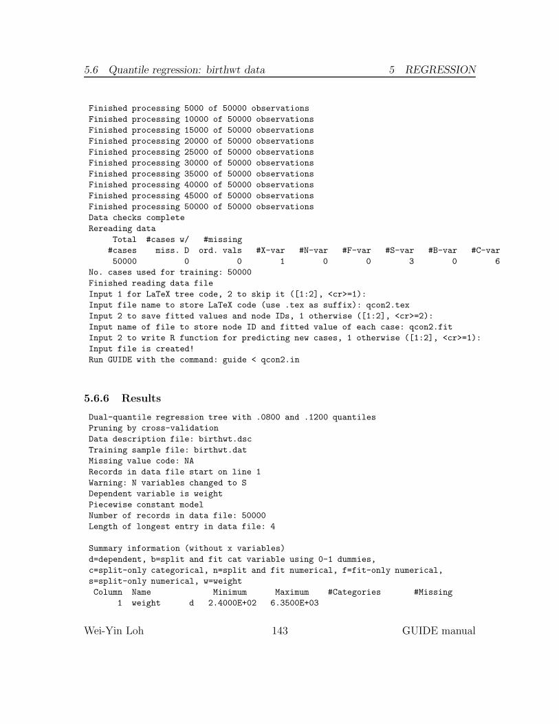
5.6 Quantile regression: birthwt data 5 REGRESSION
Finished processing 5000 of 50000 observations
Finished processing 10000 of 50000 observations
Finished processing 15000 of 50000 observations
Finished processing 20000 of 50000 observations
Finished processing 25000 of 50000 observations
Finished processing 30000 of 50000 observations
Finished processing 35000 of 50000 observations
Finished processing 40000 of 50000 observations
Finished processing 45000 of 50000 observations
Finished processing 50000 of 50000 observations
Data checks complete
Rereading data
Total #cases w/ #missing
#cases miss. D ord. vals #X-var #N-var #F-var #S-var #B-var #C-var
50000 0 0 1 0 0 3 0 6
No. cases used for training: 50000
Finished reading data file
Input 1 for LaTeX tree code, 2 to skip it ([1:2], <cr>=1):
Input file name to store LaTeX code (use .tex as suffix): qcon2.tex
Input 2 to save fitted values and node IDs, 1 otherwise ([1:2], <cr>=2):
Input name of file to store node ID and fitted value of each case: qcon2.fit
Input 2 to write R function for predicting new cases, 1 otherwise ([1:2], <cr>=1):
Input file is created!
Run GUIDE with the command: guide < qcon2.in
5.6.6 Results
Dual-quantile regression tree with .0800 and .1200 quantiles
Pruning by cross-validation
Data description file: birthwt.dsc
Training sample file: birthwt.dat
Missing value code: NA
Records in data file start on line 1
Warning: N variables changed to S
Dependent variable is weight
Piecewise constant model
Number of records in data file: 50000
Length of longest entry in data file: 4
Summary information (without x variables)
d=dependent, b=split and fit cat variable using 0-1 dummies,
c=split-only categorical, n=split and fit numerical, f=fit-only numerical,
s=split-only numerical, w=weight
Column Name Minimum Maximum #Categories #Missing
1 weight d 2.4000E+02 6.3500E+03
Wei-Yin Loh 143 GUIDE manual

5.6 Quantile regression: birthwt data 5 REGRESSION
2 black c 2
3 married c 2
4 boy c 2
5 age s 1.8000E+01 4.5000E+01
6 smoke c 2
7 cigsper s 0.0000E+00 6.0000E+01
8 wtgain s 0.0000E+00 9.8000E+01
9 visit c 4
10 ed c 4
Total #cases w/ #missing
#cases miss. D ord. vals #X-var #N-var #F-var #S-var #B-var #C-var
50000 0 0 1 0 0 3 0 6
No. cases used for training: 50000
Interaction tests on all variables
Pruning by v-fold cross-validation, with v = 10
Selected tree is based on mean of CV estimates
Fraction of cases used for splitting each node: 1.0000
Max. number of split levels: 30
Min. node sample size: 250
Number of SE’s for pruned tree: 5.0000E-01
Size and CV Loss and SE of subtrees:
Tree #Tnodes Mean Loss SE(Mean) BSE(Mean) Median Loss BSE(Median)
1 144 2.061E+02 1.432E+00 1.000E+00 2.062E+02 7.925E-01
2 141 2.061E+02 1.432E+00 9.999E-01 2.062E+02 7.913E-01
3 140 2.061E+02 1.432E+00 9.999E-01 2.062E+02 7.913E-01
4 139 2.061E+02 1.432E+00 9.999E-01 2.062E+02 7.913E-01
5 138 2.061E+02 1.432E+00 9.999E-01 2.062E+02 7.913E-01
6 137 2.061E+02 1.432E+00 9.999E-01 2.062E+02 7.913E-01
7 136 2.061E+02 1.432E+00 1.000E+00 2.062E+02 7.917E-01
8 134 2.061E+02 1.432E+00 1.000E+00 2.062E+02 7.917E-01
9 133 2.061E+02 1.432E+00 1.002E+00 2.062E+02 7.919E-01
10 132 2.061E+02 1.432E+00 1.001E+00 2.062E+02 7.906E-01
11 131 2.061E+02 1.432E+00 1.002E+00 2.062E+02 7.880E-01
12 130 2.061E+02 1.432E+00 1.002E+00 2.062E+02 7.918E-01
13 129 2.061E+02 1.432E+00 1.004E+00 2.062E+02 7.922E-01
14 127 2.061E+02 1.433E+00 1.003E+00 2.062E+02 7.884E-01
15 126 2.061E+02 1.432E+00 1.000E+00 2.062E+02 7.884E-01
16 123 2.061E+02 1.432E+00 1.000E+00 2.062E+02 7.925E-01
17 122 2.061E+02 1.432E+00 1.001E+00 2.062E+02 7.948E-01
18 121 2.061E+02 1.433E+00 1.002E+00 2.062E+02 7.957E-01
19 120 2.061E+02 1.433E+00 1.001E+00 2.061E+02 7.935E-01
20 118 2.061E+02 1.433E+00 9.954E-01 2.061E+02 7.931E-01
21 117 2.061E+02 1.433E+00 9.966E-01 2.061E+02 7.935E-01
Wei-Yin Loh 144 GUIDE manual

5.6 Quantile regression: birthwt data 5 REGRESSION
22 116 2.061E+02 1.433E+00 9.966E-01 2.061E+02 7.935E-01
23 115 2.061E+02 1.433E+00 9.966E-01 2.061E+02 7.937E-01
24 112 2.061E+02 1.433E+00 1.001E+00 2.061E+02 7.951E-01
25 111 2.061E+02 1.433E+00 1.001E+00 2.061E+02 7.946E-01
26 110 2.061E+02 1.433E+00 1.002E+00 2.061E+02 7.959E-01
27 109 2.061E+02 1.433E+00 1.002E+00 2.061E+02 7.959E-01
28 108 2.061E+02 1.432E+00 1.002E+00 2.061E+02 7.964E-01
29 107 2.061E+02 1.432E+00 1.004E+00 2.061E+02 7.869E-01
30 106 2.061E+02 1.433E+00 1.016E+00 2.062E+02 7.868E-01
31 105 2.061E+02 1.433E+00 1.024E+00 2.062E+02 7.898E-01
32 104 2.061E+02 1.433E+00 1.022E+00 2.062E+02 7.867E-01
33 101 2.061E+02 1.433E+00 1.023E+00 2.062E+02 7.877E-01
34 100 2.061E+02 1.433E+00 1.023E+00 2.063E+02 7.960E-01
35 99 2.061E+02 1.433E+00 1.023E+00 2.062E+02 8.087E-01
36 98 2.061E+02 1.433E+00 1.029E+00 2.062E+02 8.093E-01
37 97 2.061E+02 1.433E+00 1.024E+00 2.062E+02 8.020E-01
38 95 2.061E+02 1.433E+00 1.027E+00 2.062E+02 8.206E-01
39 94 2.061E+02 1.433E+00 1.027E+00 2.062E+02 8.182E-01
40 93 2.061E+02 1.433E+00 1.028E+00 2.062E+02 8.183E-01
41 92 2.061E+02 1.433E+00 1.037E+00 2.062E+02 8.264E-01
42 90 2.061E+02 1.433E+00 1.038E+00 2.062E+02 8.131E-01
43 89 2.061E+02 1.433E+00 1.038E+00 2.062E+02 7.990E-01
44 84 2.061E+02 1.433E+00 1.038E+00 2.062E+02 7.990E-01
45 83 2.062E+02 1.433E+00 1.034E+00 2.062E+02 7.987E-01
46 82 2.061E+02 1.433E+00 1.038E+00 2.062E+02 8.086E-01
47 81 2.061E+02 1.433E+00 1.038E+00 2.062E+02 8.085E-01
48 80 2.061E+02 1.433E+00 1.031E+00 2.062E+02 8.162E-01
49 79 2.061E+02 1.433E+00 1.032E+00 2.062E+02 8.275E-01
50 78 2.061E+02 1.433E+00 1.024E+00 2.063E+02 8.133E-01
51 73 2.061E+02 1.433E+00 1.024E+00 2.062E+02 7.949E-01
52 72 2.061E+02 1.432E+00 1.030E+00 2.063E+02 8.044E-01
53 71 2.061E+02 1.432E+00 1.031E+00 2.063E+02 8.158E-01
54 70 2.060E+02 1.432E+00 1.031E+00 2.063E+02 8.215E-01
55 69 2.060E+02 1.432E+00 1.030E+00 2.062E+02 8.154E-01
56 68 2.060E+02 1.431E+00 1.021E+00 2.062E+02 8.038E-01
57 67 2.060E+02 1.431E+00 1.029E+00 2.062E+02 8.124E-01
58 66 2.059E+02 1.431E+00 1.002E+00 2.061E+02 8.386E-01
59 65 2.059E+02 1.431E+00 9.977E-01 2.061E+02 8.382E-01
60 63 2.058E+02 1.430E+00 9.907E-01 2.060E+02 8.633E-01
61 61 2.058E+02 1.430E+00 1.002E+00 2.060E+02 8.681E-01
62 60 2.058E+02 1.430E+00 1.002E+00 2.060E+02 8.681E-01
63 59 2.058E+02 1.430E+00 1.007E+00 2.059E+02 8.755E-01
64 57 2.058E+02 1.431E+00 1.006E+00 2.058E+02 8.686E-01
65 56 2.058E+02 1.431E+00 1.005E+00 2.059E+02 8.562E-01
66 55 2.058E+02 1.431E+00 1.007E+00 2.059E+02 8.535E-01
67 54 2.058E+02 1.431E+00 1.004E+00 2.059E+02 8.443E-01
Wei-Yin Loh 145 GUIDE manual

5.6 Quantile regression: birthwt data 5 REGRESSION
68 53 2.057E+02 1.430E+00 9.969E-01 2.059E+02 8.294E-01
69 51 2.057E+02 1.430E+00 9.982E-01 2.058E+02 8.429E-01
70 50 2.057E+02 1.430E+00 9.902E-01 2.058E+02 8.603E-01
71 47 2.057E+02 1.430E+00 9.902E-01 2.058E+02 8.603E-01
72 45 2.057E+02 1.431E+00 9.990E-01 2.057E+02 8.871E-01
73 44 2.057E+02 1.432E+00 9.956E-01 2.057E+02 8.740E-01
74 42 2.057E+02 1.432E+00 1.012E+00 2.057E+02 9.337E-01
75 41 2.057E+02 1.433E+00 1.034E+00 2.057E+02 9.456E-01
76 39 2.057E+02 1.433E+00 1.040E+00 2.057E+02 9.452E-01
77 37 2.057E+02 1.433E+00 1.042E+00 2.057E+02 9.631E-01
78 35 2.057E+02 1.433E+00 1.040E+00 2.057E+02 9.738E-01
79 34 2.057E+02 1.433E+00 1.042E+00 2.057E+02 9.784E-01
80 31 2.057E+02 1.434E+00 1.048E+00 2.057E+02 9.802E-01
81 28 2.057E+02 1.435E+00 1.060E+00 2.057E+02 9.967E-01
82 26 2.057E+02 1.435E+00 1.060E+00 2.057E+02 9.968E-01
83 25 2.057E+02 1.436E+00 1.057E+00 2.057E+02 1.002E+00
84* 24 2.056E+02 1.436E+00 1.074E+00 2.056E+02 1.094E+00
85 23 2.057E+02 1.436E+00 1.076E+00 2.058E+02 1.088E+00
86 22 2.057E+02 1.436E+00 1.075E+00 2.058E+02 1.083E+00
87 21 2.057E+02 1.438E+00 1.097E+00 2.058E+02 1.013E+00
88 20 2.058E+02 1.438E+00 1.055E+00 2.057E+02 9.310E-01
89 19 2.058E+02 1.437E+00 1.041E+00 2.059E+02 8.785E-01
90 16 2.059E+02 1.440E+00 1.050E+00 2.060E+02 8.878E-01
91 15 2.060E+02 1.440E+00 1.055E+00 2.060E+02 9.370E-01
92++ 14 2.059E+02 1.439E+00 1.043E+00 2.060E+02 9.050E-01
93 13 2.062E+02 1.440E+00 1.015E+00 2.065E+02 7.956E-01
94-- 12 2.061E+02 1.439E+00 1.007E+00 2.064E+02 8.030E-01
95** 11 2.063E+02 1.439E+00 1.036E+00 2.067E+02 8.540E-01
96 10 2.064E+02 1.440E+00 1.030E+00 2.069E+02 8.662E-01
97 8 2.064E+02 1.440E+00 1.031E+00 2.069E+02 8.684E-01
98 7 2.067E+02 1.438E+00 1.028E+00 2.069E+02 8.015E-01
99 6 2.070E+02 1.444E+00 9.629E-01 2.073E+02 7.845E-01
100 5 2.073E+02 1.448E+00 8.978E-01 2.076E+02 7.698E-01
101 4 2.091E+02 1.456E+00 1.115E+00 2.099E+02 1.238E+00
102 3 2.100E+02 1.463E+00 8.880E-01 2.103E+02 8.149E-01
103 2 2.122E+02 1.486E+00 1.002E+00 2.128E+02 9.149E-01
104 1 2.173E+02 1.576E+00 1.015E+00 2.178E+02 1.229E+00
0-SE tree based on mean is marked with * and has 24 terminal nodes
0-SE tree based on median is marked with + and has 24 terminal nodes
Selected-SE tree based on mean using naive SE is marked with **
Selected-SE tree based on mean using bootstrap SE is marked with --
Selected-SE tree based on median and bootstrap SE is marked with ++
* tree same as + tree
Following tree is based on mean CV with naive SE estimate (**).
Wei-Yin Loh 146 GUIDE manual
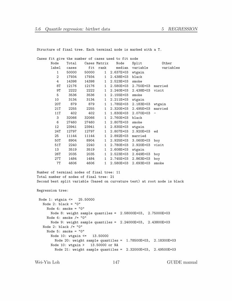
5.6 Quantile regression: birthwt data 5 REGRESSION
Structure of final tree. Each terminal node is marked with a T.
Cases fit give the number of cases used to fit node
Node Total Cases Matrix Node Split Other
label cases fit rank median variable variables
1 50000 50000 1 2.637E+03 wtgain
2 17934 17934 1 2.438E+03 black
4 14398 14398 1 2.523E+03 smoke
8T 12176 12176 1 2.580E+03 2.750E+03 married
9T 2222 2222 1 2.240E+03 2.438E+03 visit
5 3536 3536 1 2.155E+03 smoke
10 3134 3134 1 2.211E+03 wtgain
20T 879 879 1 1.785E+03 2.183E+03 wtgain
21T 2255 2255 1 2.320E+03 2.495E+03 married
11T 402 402 1 1.830E+03 2.070E+03 -
3 32066 32066 1 2.760E+03 black
6 27460 27460 1 2.807E+03 smoke
12 23941 23941 1 2.835E+03 wtgain
24T 12797 12797 1 2.807E+03 2.920E+03 ed
25 11144 11144 1 2.892E+03 married
50T 8904 8904 1 2.925E+03 3.060E+03 boy
51T 2240 2240 1 2.780E+03 2.920E+03 visit
13 3519 3519 1 2.608E+03 wtgain
26T 2035 2035 1 2.523E+03 2.649E+03 boy
27T 1484 1484 1 2.745E+03 2.863E+03 boy
7T 4606 4606 1 2.580E+03 2.693E+03 smoke
Number of terminal nodes of final tree: 11
Total number of nodes of final tree: 21
Second best split variable (based on curvature test) at root node is black
Regression tree:
Node 1: wtgain <= 25.50000
Node 2: black = "0"
Node 4: smoke = "0"
Node 8: weight sample quantiles = 2.58000E+03, 2.75000E+03
Node 4: smoke /= "0"
Node 9: weight sample quantiles = 2.24000E+03, 2.43800E+03
Node 2: black /= "0"
Node 5: smoke = "0"
Node 10: wtgain <= 13.50000
Node 20: weight sample quantiles = 1.78500E+03, 2.18300E+03
Node 10: wtgain > 13.50000 or NA
Node 21: weight sample quantiles = 2.32000E+03, 2.49500E+03
Wei-Yin Loh 147 GUIDE manual

5.6 Quantile regression: birthwt data 5 REGRESSION
Node 5: smoke /= "0"
Node 11: weight sample quantiles = 1.83000E+03, 2.07000E+03
Node 1: wtgain > 25.50000 or NA
Node 3: black = "0"
Node 6: smoke = "0"
Node 12: wtgain <= 35.50000 or NA
Node 24: weight sample quantiles = 2.80700E+03, 2.92000E+03
Node 12: wtgain > 35.50000
Node 25: married = "1"
Node 50: weight sample quantiles = 2.92500E+03, 3.06000E+03
Node 25: married /= "1"
Node 51: weight sample quantiles = 2.78000E+03, 2.92000E+03
Node 6: smoke /= "0"
Node 13: wtgain <= 39.50000 or NA
Node 26: weight sample quantiles = 2.52300E+03, 2.64900E+03
Node 13: wtgain > 39.50000
Node 27: weight sample quantiles = 2.74500E+03, 2.86300E+03
Node 3: black /= "0"
Node 7: weight sample quantiles = 2.58000E+03, 2.69300E+03
***************************************************************
WARNING: p-values below are not adjusted for split search. For a bootstrap
solution, see Loh et al. (2016), "Identification of subgroups with
differential treatment effects for longitudinal and multiresponse
variables", Statistics in Medicine, v.35, 4837-4855.
Node 1: Intermediate node
A case goes into Node 2 if wtgain <= 2.5500000E+01
wtgain mean = 3.0709E+01
Sample lower quantile, median, and upper quantile:
2.6370E+03 2.8000E+03 3.4020E+03
The three numbers above are the 0.08, 0.12 and 0.50 quantiles.
----------------------------
Node 2: Intermediate node
A case goes into Node 4 if black = "0"
black mode = "0"
----------------------------
Node 4: Intermediate node
A case goes into Node 8 if smoke = "0"
smoke mode = "0"
----------------------------
Node 8: Terminal node
Sample lower quantile, median, and upper quantile:
2.5800E+03 2.7500E+03 3.3740E+03
Wei-Yin Loh 148 GUIDE manual
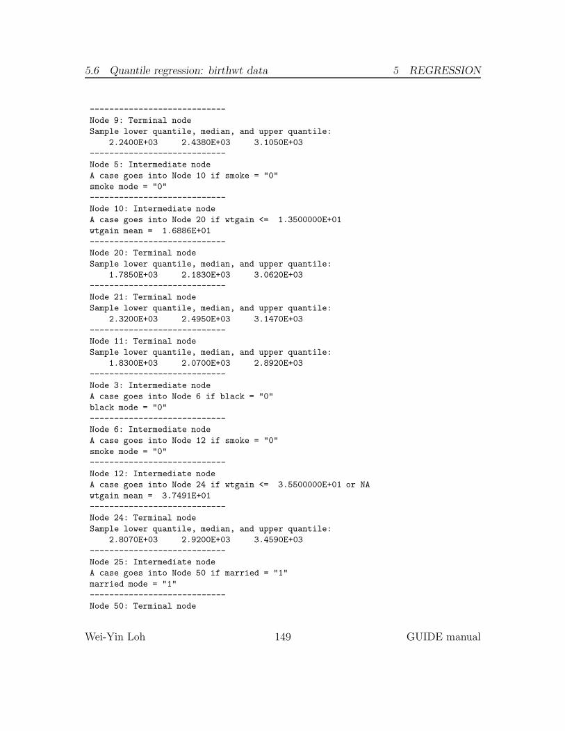
5.6 Quantile regression: birthwt data 5 REGRESSION
----------------------------
Node 9: Terminal node
Sample lower quantile, median, and upper quantile:
2.2400E+03 2.4380E+03 3.1050E+03
----------------------------
Node 5: Intermediate node
A case goes into Node 10 if smoke = "0"
smoke mode = "0"
----------------------------
Node 10: Intermediate node
A case goes into Node 20 if wtgain <= 1.3500000E+01
wtgain mean = 1.6886E+01
----------------------------
Node 20: Terminal node
Sample lower quantile, median, and upper quantile:
1.7850E+03 2.1830E+03 3.0620E+03
----------------------------
Node 21: Terminal node
Sample lower quantile, median, and upper quantile:
2.3200E+03 2.4950E+03 3.1470E+03
----------------------------
Node 11: Terminal node
Sample lower quantile, median, and upper quantile:
1.8300E+03 2.0700E+03 2.8920E+03
----------------------------
Node 3: Intermediate node
A case goes into Node 6 if black = "0"
black mode = "0"
----------------------------
Node 6: Intermediate node
A case goes into Node 12 if smoke = "0"
smoke mode = "0"
----------------------------
Node 12: Intermediate node
A case goes into Node 24 if wtgain <= 3.5500000E+01 or NA
wtgain mean = 3.7491E+01
----------------------------
Node 24: Terminal node
Sample lower quantile, median, and upper quantile:
2.8070E+03 2.9200E+03 3.4590E+03
----------------------------
Node 25: Intermediate node
A case goes into Node 50 if married = "1"
married mode = "1"
----------------------------
Node 50: Terminal node
Wei-Yin Loh 149 GUIDE manual
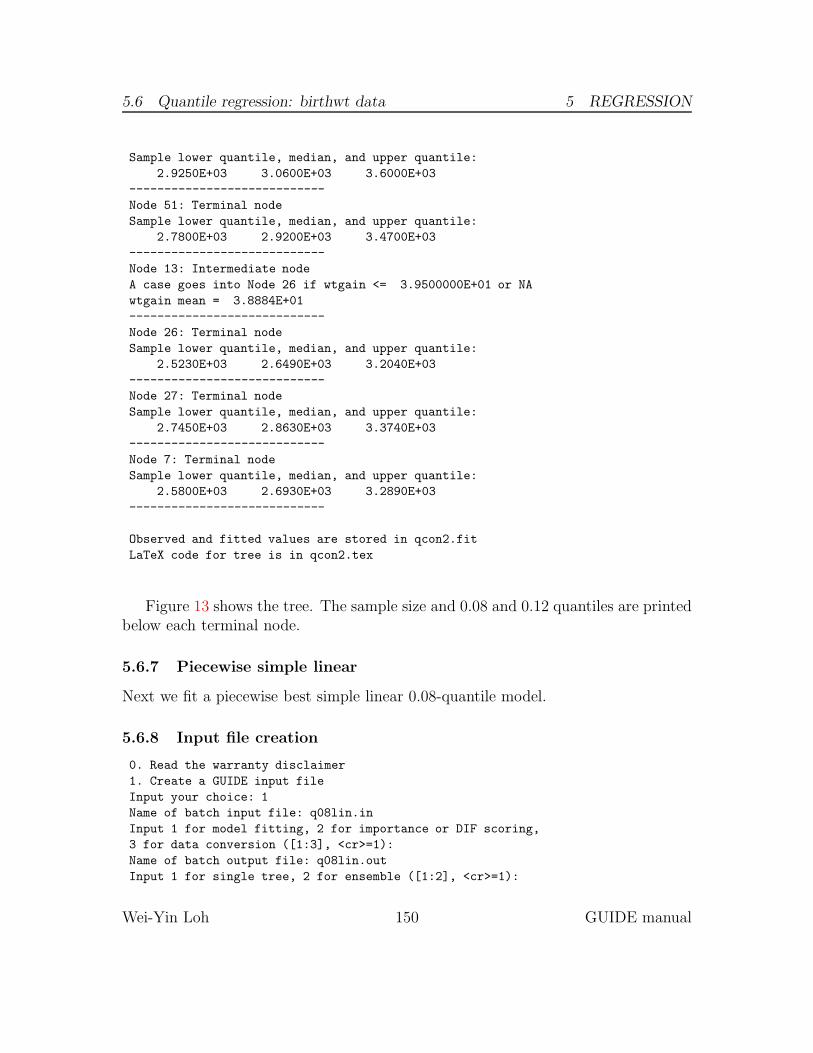
5.6 Quantile regression: birthwt data 5 REGRESSION
Sample lower quantile, median, and upper quantile:
2.9250E+03 3.0600E+03 3.6000E+03
----------------------------
Node 51: Terminal node
Sample lower quantile, median, and upper quantile:
2.7800E+03 2.9200E+03 3.4700E+03
----------------------------
Node 13: Intermediate node
A case goes into Node 26 if wtgain <= 3.9500000E+01 or NA
wtgain mean = 3.8884E+01
----------------------------
Node 26: Terminal node
Sample lower quantile, median, and upper quantile:
2.5230E+03 2.6490E+03 3.2040E+03
----------------------------
Node 27: Terminal node
Sample lower quantile, median, and upper quantile:
2.7450E+03 2.8630E+03 3.3740E+03
----------------------------
Node 7: Terminal node
Sample lower quantile, median, and upper quantile:
2.5800E+03 2.6930E+03 3.2890E+03
----------------------------
Observed and fitted values are stored in qcon2.fit
LaTeX code for tree is in qcon2.tex
Figure 13 shows the tree. The sample size and 0.08 and 0.12 quantiles are printedbelow each terminal node.
5.6.7 Piecewise simple linear
Next we fit a piecewise best simple linear 0.08-quantile model.
5.6.8 Input file creation
0. Read the warranty disclaimer
1. Create a GUIDE input file
Input your choice: 1
Name of batch input file: q08lin.in
Input 1 for model fitting, 2 for importance or DIF scoring,
3 for data conversion ([1:3], <cr>=1):
Name of batch output file: q08lin.out
Input 1 for single tree, 2 for ensemble ([1:2], <cr>=1):
Wei-Yin Loh 150 GUIDE manual

5.6 Quantile regression: birthwt data 5 REGRESSION
wtgain≤ 25.50 1
black= 0 2
smoke= 0 4
8
121762750.2580.
9
22222438.2240.
smoke= 0 5
wtgain≤ 13.50 10
20
8792183.1785.
21
22552495.2320.
11
4022070.1830.
black= 0 3
smoke= 0 6
wtgain≤∗35.50 12
24
127972920.2807.
married= 1 25
50
89043060.2925.
51
22402920.2780.
wtgain≤∗39.50 13
26
20352649.2523.
27
14842863.2745.
7
46062693.2580.
Figure 13: GUIDE v.27.9 0.50-SE piecewise constant 0.08 and 0.12-quantile regres-sion tree for predicting weight. Maximum number of split levels is 30 and minimumnode sample size is 250. At each split, an observation goes to the left branch if andonly if the condition is satisfied. The symbol ‘≤∗’ stands for ‘≤ or missing’. Samplesize (in italics) and sample 0.12 and 0.08-quantiles of weight printed below nodes.Second best split variable at root node is black.
Wei-Yin Loh 151 GUIDE manual
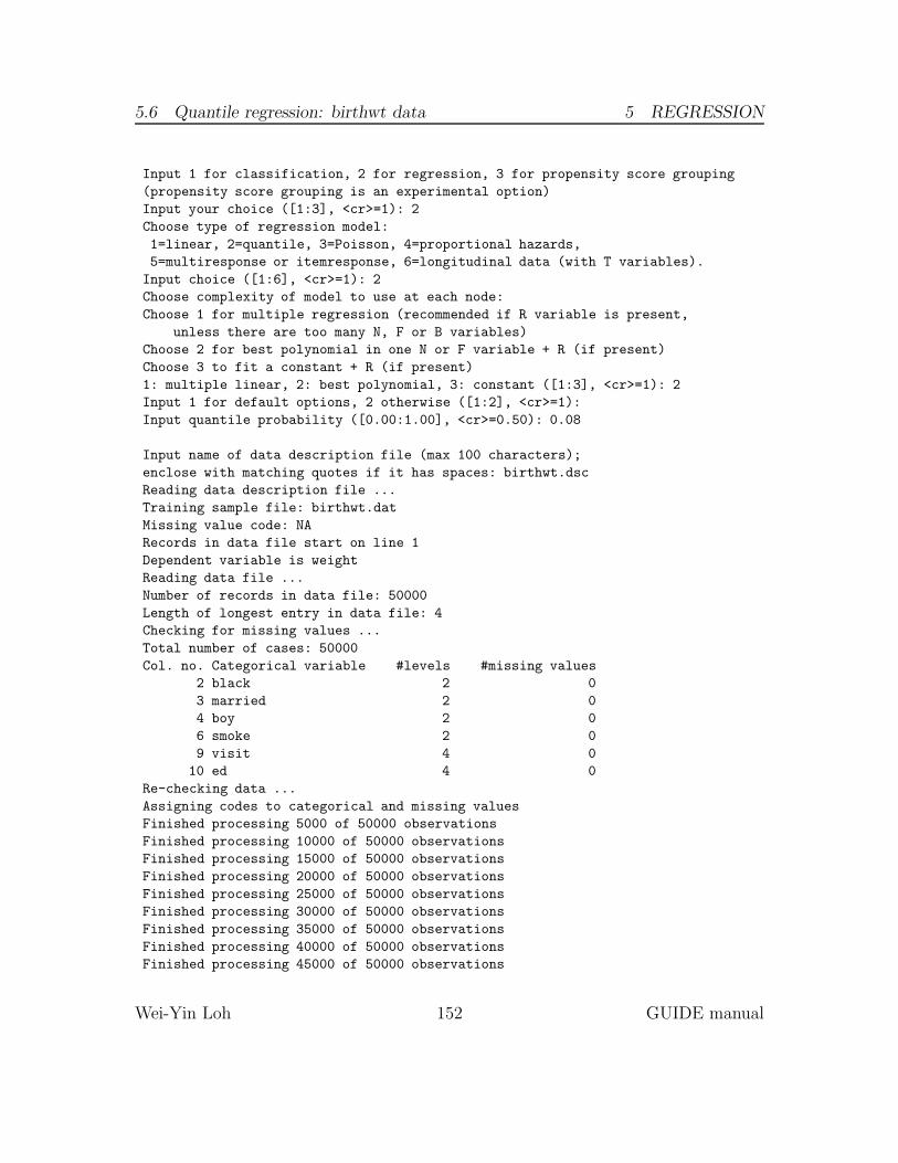
5.6 Quantile regression: birthwt data 5 REGRESSION
Input 1 for classification, 2 for regression, 3 for propensity score grouping
(propensity score grouping is an experimental option)
Input your choice ([1:3], <cr>=1): 2
Choose type of regression model:
1=linear, 2=quantile, 3=Poisson, 4=proportional hazards,
5=multiresponse or itemresponse, 6=longitudinal data (with T variables).
Input choice ([1:6], <cr>=1): 2
Choose complexity of model to use at each node:
Choose 1 for multiple regression (recommended if R variable is present,
unless there are too many N, F or B variables)
Choose 2 for best polynomial in one N or F variable + R (if present)
Choose 3 to fit a constant + R (if present)
1: multiple linear, 2: best polynomial, 3: constant ([1:3], <cr>=1): 2
Input 1 for default options, 2 otherwise ([1:2], <cr>=1):
Input quantile probability ([0.00:1.00], <cr>=0.50): 0.08
Input name of data description file (max 100 characters);
enclose with matching quotes if it has spaces: birthwt.dsc
Reading data description file ...
Training sample file: birthwt.dat
Missing value code: NA
Records in data file start on line 1
Dependent variable is weight
Reading data file ...
Number of records in data file: 50000
Length of longest entry in data file: 4
Checking for missing values ...
Total number of cases: 50000
Col. no. Categorical variable #levels #missing values
2 black 2 0
3 married 2 0
4 boy 2 0
6 smoke 2 0
9 visit 4 0
10 ed 4 0
Re-checking data ...
Assigning codes to categorical and missing values
Finished processing 5000 of 50000 observations
Finished processing 10000 of 50000 observations
Finished processing 15000 of 50000 observations
Finished processing 20000 of 50000 observations
Finished processing 25000 of 50000 observations
Finished processing 30000 of 50000 observations
Finished processing 35000 of 50000 observations
Finished processing 40000 of 50000 observations
Finished processing 45000 of 50000 observations
Wei-Yin Loh 152 GUIDE manual

5.6 Quantile regression: birthwt data 5 REGRESSION
Finished processing 50000 of 50000 observations
Data checks complete
Rereading data
Total #cases w/ #missing
#cases miss. D ord. vals #X-var #N-var #F-var #S-var #B-var #C-var
50000 0 0 1 3 0 0 0 6
No. cases used for training: 50000
Finished reading data file
Input 1 for LaTeX tree code, 2 to skip it ([1:2], <cr>=1):
Input file name to store LaTeX code (use .tex as suffix): q08lin.tex
Input 2 to save fitted values and node IDs, 1 otherwise ([1:2], <cr>=2):
Input name of file to store node ID and fitted value of each case: q08lin.fit
Input 2 to write R function for predicting new cases, 1 otherwise ([1:2], <cr>=1):
Input file is created!
Run GUIDE with the command: guide < q08lin.in
5.6.9 Results
Quantile regression tree with quantile probability .0800
No truncation of predicted values
Pruning by cross-validation
Data description file: birthwt.dsc
Training sample file: birthwt.dat
Missing value code: NA
Records in data file start on line 1
Dependent variable is weight
Piecewise simple linear or constant model
Powers are dropped if they are not significant at level 1.0000
Number of records in data file: 50000
Length of longest entry in data file: 4
Summary information (without x variables)
d=dependent, b=split and fit cat variable using 0-1 dummies,
c=split-only categorical, n=split and fit numerical, f=fit-only numerical,
s=split-only numerical, w=weight
Column Name Minimum Maximum #Categories #Missing
1 weight d 2.4000E+02 6.3500E+03
2 black c 2
3 married c 2
4 boy c 2
5 age n 1.8000E+01 4.5000E+01
6 smoke c 2
7 cigsper n 0.0000E+00 6.0000E+01
8 wtgain n 0.0000E+00 9.8000E+01
9 visit c 4
Wei-Yin Loh 153 GUIDE manual
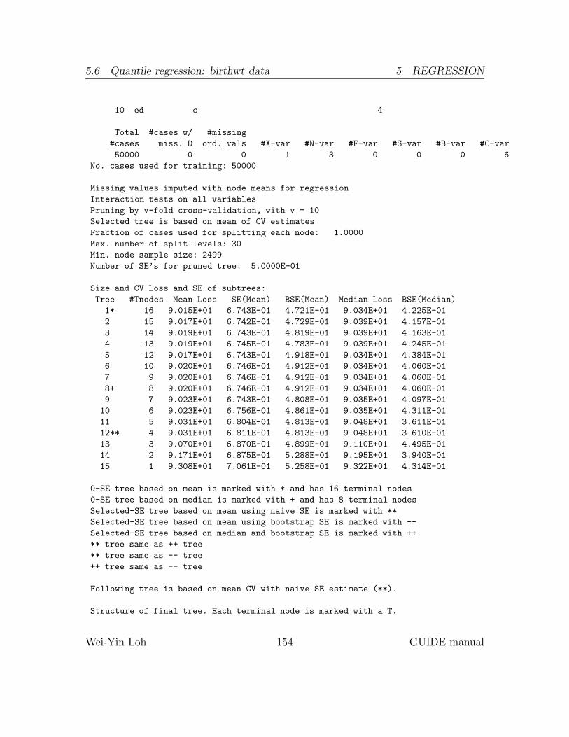
5.6 Quantile regression: birthwt data 5 REGRESSION
10 ed c 4
Total #cases w/ #missing
#cases miss. D ord. vals #X-var #N-var #F-var #S-var #B-var #C-var
50000 0 0 1 3 0 0 0 6
No. cases used for training: 50000
Missing values imputed with node means for regression
Interaction tests on all variables
Pruning by v-fold cross-validation, with v = 10
Selected tree is based on mean of CV estimates
Fraction of cases used for splitting each node: 1.0000
Max. number of split levels: 30
Min. node sample size: 2499
Number of SE’s for pruned tree: 5.0000E-01
Size and CV Loss and SE of subtrees:
Tree #Tnodes Mean Loss SE(Mean) BSE(Mean) Median Loss BSE(Median)
1* 16 9.015E+01 6.743E-01 4.721E-01 9.034E+01 4.225E-01
2 15 9.017E+01 6.742E-01 4.729E-01 9.039E+01 4.157E-01
3 14 9.019E+01 6.743E-01 4.819E-01 9.039E+01 4.163E-01
4 13 9.019E+01 6.745E-01 4.783E-01 9.039E+01 4.245E-01
5 12 9.017E+01 6.743E-01 4.918E-01 9.034E+01 4.384E-01
6 10 9.020E+01 6.746E-01 4.912E-01 9.034E+01 4.060E-01
7 9 9.020E+01 6.746E-01 4.912E-01 9.034E+01 4.060E-01
8+ 8 9.020E+01 6.746E-01 4.912E-01 9.034E+01 4.060E-01
9 7 9.023E+01 6.743E-01 4.808E-01 9.035E+01 4.097E-01
10 6 9.023E+01 6.756E-01 4.861E-01 9.035E+01 4.311E-01
11 5 9.031E+01 6.804E-01 4.813E-01 9.048E+01 3.611E-01
12** 4 9.031E+01 6.811E-01 4.813E-01 9.048E+01 3.610E-01
13 3 9.070E+01 6.870E-01 4.899E-01 9.110E+01 4.495E-01
14 2 9.171E+01 6.875E-01 5.288E-01 9.195E+01 3.940E-01
15 1 9.308E+01 7.061E-01 5.258E-01 9.322E+01 4.314E-01
0-SE tree based on mean is marked with * and has 16 terminal nodes
0-SE tree based on median is marked with + and has 8 terminal nodes
Selected-SE tree based on mean using naive SE is marked with **
Selected-SE tree based on mean using bootstrap SE is marked with --
Selected-SE tree based on median and bootstrap SE is marked with ++
** tree same as ++ tree
** tree same as -- tree
++ tree same as -- tree
Following tree is based on mean CV with naive SE estimate (**).
Structure of final tree. Each terminal node is marked with a T.
Wei-Yin Loh 154 GUIDE manual

5.6 Quantile regression: birthwt data 5 REGRESSION
D-quant is quantile of weight in the node
Cases fit give the number of cases used to fit node
Node Total Cases Matrix Node Split Other
label cases fit rank D-quant variable variables
1 50000 50000 2 2.637E+03 black
2T 8142 8142 2 2.381E+03 wtgain
3 41858 41858 2 2.710E+03 smoke
6T 5741 5741 2 2.466E+03 boy
7 36117 36117 2 2.750E+03 married
14T 6484 6484 2 2.637E+03 wtgain
15T 29633 29633 2 2.778E+03 age
Number of terminal nodes of final tree: 4
Total number of nodes of final tree: 7
Second best split variable (based on curvature test) at root node is married
Regression tree:
Node 1: black = "1"
Node 2: weight sample quantile = 2.38100E+03
Node 1: black /= "1"
Node 3: smoke = "1"
Node 6: weight sample quantile = 2.46600E+03
Node 3: smoke /= "1"
Node 7: married = "0"
Node 14: weight sample quantile = 2.63700E+03
Node 7: married /= "0"
Node 15: weight sample quantile = 2.77800E+03
***************************************************************
WARNING: p-values below are not adjusted for split search. For a bootstrap
solution, see Loh et al. (2016), "Identification of subgroups with
differential treatment effects for longitudinal and multiresponse
variables", Statistics in Medicine, v.35, 4837-4855.
Node 1: Intermediate node
A case goes into Node 2 if black = "1"
black mode = "0"
Coefficients of quantile regression function:
Regressor Coefficient Minimum Mean Maximum
Constant 2.3027E+03
wtgain 1.1333E+01 0.0000E+00 3.0709E+01 9.8000E+01
----------------------------
Wei-Yin Loh 155 GUIDE manual
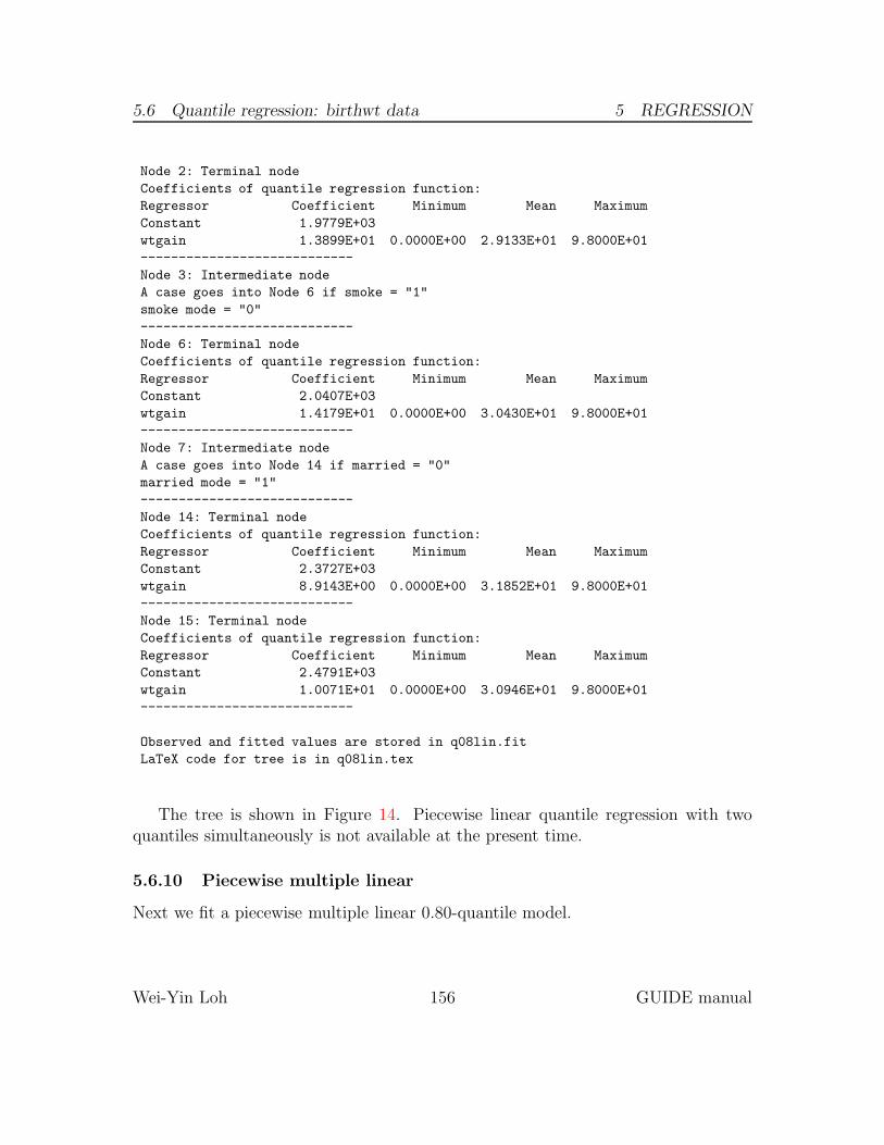
5.6 Quantile regression: birthwt data 5 REGRESSION
Node 2: Terminal node
Coefficients of quantile regression function:
Regressor Coefficient Minimum Mean Maximum
Constant 1.9779E+03
wtgain 1.3899E+01 0.0000E+00 2.9133E+01 9.8000E+01
----------------------------
Node 3: Intermediate node
A case goes into Node 6 if smoke = "1"
smoke mode = "0"
----------------------------
Node 6: Terminal node
Coefficients of quantile regression function:
Regressor Coefficient Minimum Mean Maximum
Constant 2.0407E+03
wtgain 1.4179E+01 0.0000E+00 3.0430E+01 9.8000E+01
----------------------------
Node 7: Intermediate node
A case goes into Node 14 if married = "0"
married mode = "1"
----------------------------
Node 14: Terminal node
Coefficients of quantile regression function:
Regressor Coefficient Minimum Mean Maximum
Constant 2.3727E+03
wtgain 8.9143E+00 0.0000E+00 3.1852E+01 9.8000E+01
----------------------------
Node 15: Terminal node
Coefficients of quantile regression function:
Regressor Coefficient Minimum Mean Maximum
Constant 2.4791E+03
wtgain 1.0071E+01 0.0000E+00 3.0946E+01 9.8000E+01
----------------------------
Observed and fitted values are stored in q08lin.fit
LaTeX code for tree is in q08lin.tex
The tree is shown in Figure 14. Piecewise linear quantile regression with twoquantiles simultaneously is not available at the present time.
5.6.10 Piecewise multiple linear
Next we fit a piecewise multiple linear 0.80-quantile model.
Wei-Yin Loh 156 GUIDE manual
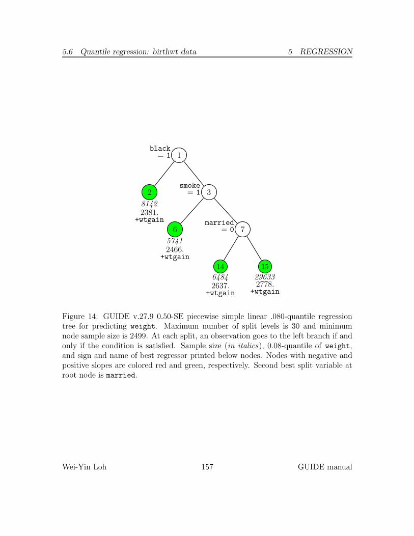
5.6 Quantile regression: birthwt data 5 REGRESSION
black= 1 1
2
81422381.
+wtgain
smoke= 1 3
6
57412466.
+wtgain
married= 0 7
14
64842637.
+wtgain
15
296332778.
+wtgain
Figure 14: GUIDE v.27.9 0.50-SE piecewise simple linear .080-quantile regressiontree for predicting weight. Maximum number of split levels is 30 and minimumnode sample size is 2499. At each split, an observation goes to the left branch if andonly if the condition is satisfied. Sample size (in italics), 0.08-quantile of weight,and sign and name of best regressor printed below nodes. Nodes with negative andpositive slopes are colored red and green, respectively. Second best split variable atroot node is married.
Wei-Yin Loh 157 GUIDE manual
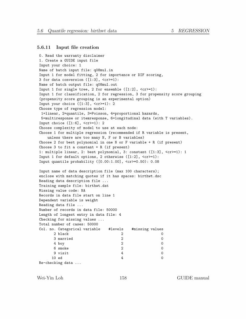
5.6 Quantile regression: birthwt data 5 REGRESSION
5.6.11 Input file creation
0. Read the warranty disclaimer
1. Create a GUIDE input file
Input your choice: 1
Name of batch input file: q08mul.in
Input 1 for model fitting, 2 for importance or DIF scoring,
3 for data conversion ([1:3], <cr>=1):
Name of batch output file: q08mul.out
Input 1 for single tree, 2 for ensemble ([1:2], <cr>=1):
Input 1 for classification, 2 for regression, 3 for propensity score grouping
(propensity score grouping is an experimental option)
Input your choice ([1:3], <cr>=1): 2
Choose type of regression model:
1=linear, 2=quantile, 3=Poisson, 4=proportional hazards,
5=multiresponse or itemresponse, 6=longitudinal data (with T variables).
Input choice ([1:6], <cr>=1): 2
Choose complexity of model to use at each node:
Choose 1 for multiple regression (recommended if R variable is present,
unless there are too many N, F or B variables)
Choose 2 for best polynomial in one N or F variable + R (if present)
Choose 3 to fit a constant + R (if present)
1: multiple linear, 2: best polynomial, 3: constant ([1:3], <cr>=1): 1
Input 1 for default options, 2 otherwise ([1:2], <cr>=1):
Input quantile probability ([0.00:1.00], <cr>=0.50): 0.08
Input name of data description file (max 100 characters);
enclose with matching quotes if it has spaces: birthwt.dsc
Reading data description file ...
Training sample file: birthwt.dat
Missing value code: NA
Records in data file start on line 1
Dependent variable is weight
Reading data file ...
Number of records in data file: 50000
Length of longest entry in data file: 4
Checking for missing values ...
Total number of cases: 50000
Col. no. Categorical variable #levels #missing values
2 black 2 0
3 married 2 0
4 boy 2 0
6 smoke 2 0
9 visit 4 0
10 ed 4 0
Re-checking data ...
Wei-Yin Loh 158 GUIDE manual

5.6 Quantile regression: birthwt data 5 REGRESSION
Assigning codes to categorical and missing values
Finished processing 5000 of 50000 observations
Finished processing 10000 of 50000 observations
Finished processing 15000 of 50000 observations
Finished processing 20000 of 50000 observations
Finished processing 25000 of 50000 observations
Finished processing 30000 of 50000 observations
Finished processing 35000 of 50000 observations
Finished processing 40000 of 50000 observations
Finished processing 45000 of 50000 observations
Finished processing 50000 of 50000 observations
Data checks complete
Rereading data
Total #cases w/ #missing
#cases miss. D ord. vals #X-var #N-var #F-var #S-var #B-var #C-var
50000 0 0 1 3 0 0 0 6
No. cases used for training: 50000
Finished reading data file
Input 1 for LaTeX tree code, 2 to skip it ([1:2], <cr>=1):
Input file name to store LaTeX code (use .tex as suffix): q08mul.tex
Input 2 to save fitted values and node IDs, 1 otherwise ([1:2], <cr>=2):
Input name of file to store node ID and fitted value of each case: q08mul.fit
Input 2 to write R function for predicting new cases, 1 otherwise ([1:2], <cr>=1):
Input file is created!
Run GUIDE with the command: guide < q08mul.in
5.6.12 Results
Quantile regression tree with quantile probability 0.0800
No truncation of predicted values
Pruning by cross-validation
Data description file: birthwt.dsc
Training sample file: birthwt.dat
Missing value code: NA
Records in data file start on line 1
Dependent variable is weight
Piecewise linear model
Number of records in data file: 50000
Length of longest entry in data file: 4
Summary information (without x variables)
d=dependent, b=split and fit cat variable using 0-1 dummies,
c=split-only categorical, n=split and fit numerical, f=fit-only numerical,
s=split-only numerical, w=weight
Column Name Minimum Maximum #Categories #Missing
Wei-Yin Loh 159 GUIDE manual
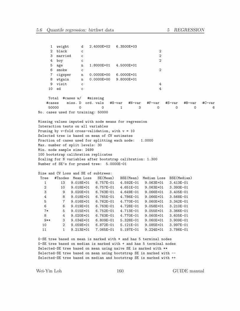
5.6 Quantile regression: birthwt data 5 REGRESSION
1 weight d 2.4000E+02 6.3500E+03
2 black c 2
3 married c 2
4 boy c 2
5 age n 1.8000E+01 4.5000E+01
6 smoke c 2
7 cigsper n 0.0000E+00 6.0000E+01
8 wtgain n 0.0000E+00 9.8000E+01
9 visit c 4
10 ed c 4
Total #cases w/ #missing
#cases miss. D ord. vals #X-var #N-var #F-var #S-var #B-var #C-var
50000 0 0 1 3 0 0 0 6
No. cases used for training: 50000
Missing values imputed with node means for regression
Interaction tests on all variables
Pruning by v-fold cross-validation, with v = 10
Selected tree is based on mean of CV estimates
Fraction of cases used for splitting each node: 1.0000
Max. number of split levels: 30
Min. node sample size: 2499
100 bootstrap calibration replicates
Scaling for N variables after bootstrap calibration: 1.300
Number of SE’s for pruned tree: 5.0000E-01
Size and CV Loss and SE of subtrees:
Tree #Tnodes Mean Loss SE(Mean) BSE(Mean) Median Loss BSE(Median)
1 13 9.018E+01 6.757E-01 4.592E-01 9.063E+01 3.413E-01
2 10 9.018E+01 6.757E-01 4.651E-01 9.063E+01 3.393E-01
3 9 9.020E+01 6.763E-01 4.649E-01 9.066E+01 3.405E-01
4 8 9.018E+01 6.765E-01 4.786E-01 9.066E+01 3.568E-01
5 7 9.016E+01 6.762E-01 4.770E-01 9.060E+01 3.342E-01
6 6 9.019E+01 6.763E-01 4.728E-01 9.058E+01 3.210E-01
7* 5 9.015E+01 6.752E-01 4.713E-01 9.055E+01 3.366E-01
8 4 9.020E+01 6.763E-01 4.770E-01 9.060E+01 3.605E-01
9** 3 9.034E+01 6.809E-01 5.328E-01 9.060E+01 3.909E-01
10 2 9.059E+01 6.872E-01 5.121E-01 9.085E+01 3.997E-01
11 1 9.213E+01 7.065E-01 5.197E-01 9.224E+01 3.786E-01
0-SE tree based on mean is marked with * and has 5 terminal nodes
0-SE tree based on median is marked with + and has 5 terminal nodes
Selected-SE tree based on mean using naive SE is marked with **
Selected-SE tree based on mean using bootstrap SE is marked with --
Selected-SE tree based on median and bootstrap SE is marked with ++
Wei-Yin Loh 160 GUIDE manual
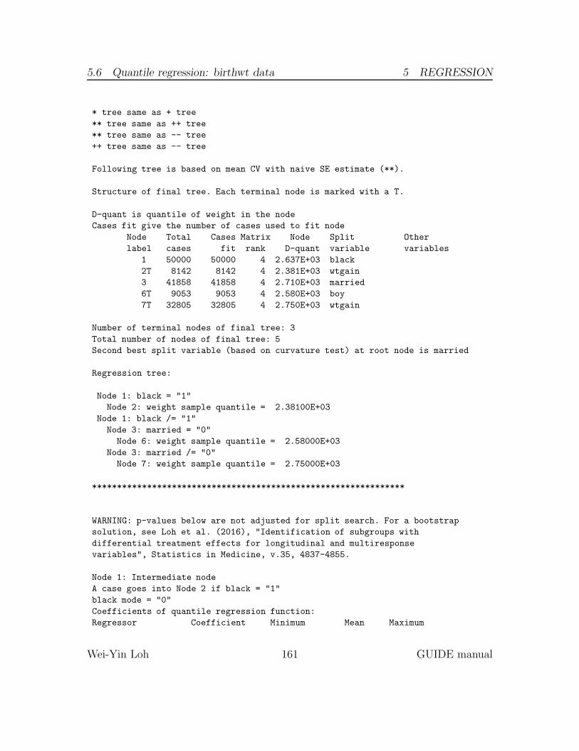
5.6 Quantile regression: birthwt data 5 REGRESSION
* tree same as + tree
** tree same as ++ tree
** tree same as -- tree
++ tree same as -- tree
Following tree is based on mean CV with naive SE estimate (**).
Structure of final tree. Each terminal node is marked with a T.
D-quant is quantile of weight in the node
Cases fit give the number of cases used to fit node
Node Total Cases Matrix Node Split Other
label cases fit rank D-quant variable variables
1 50000 50000 4 2.637E+03 black
2T 8142 8142 4 2.381E+03 wtgain
3 41858 41858 4 2.710E+03 married
6T 9053 9053 4 2.580E+03 boy
7T 32805 32805 4 2.750E+03 wtgain
Number of terminal nodes of final tree: 3
Total number of nodes of final tree: 5
Second best split variable (based on curvature test) at root node is married
Regression tree:
Node 1: black = "1"
Node 2: weight sample quantile = 2.38100E+03
Node 1: black /= "1"
Node 3: married = "0"
Node 6: weight sample quantile = 2.58000E+03
Node 3: married /= "0"
Node 7: weight sample quantile = 2.75000E+03
***************************************************************
WARNING: p-values below are not adjusted for split search. For a bootstrap
solution, see Loh et al. (2016), "Identification of subgroups with
differential treatment effects for longitudinal and multiresponse
variables", Statistics in Medicine, v.35, 4837-4855.
Node 1: Intermediate node
A case goes into Node 2 if black = "1"
black mode = "0"
Coefficients of quantile regression function:
Regressor Coefficient Minimum Mean Maximum
Wei-Yin Loh 161 GUIDE manual
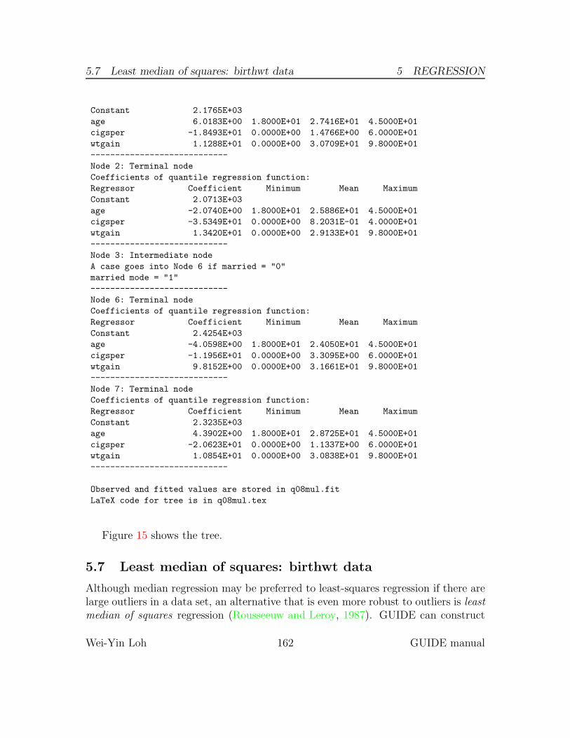
5.7 Least median of squares: birthwt data 5 REGRESSION
Constant 2.1765E+03
age 6.0183E+00 1.8000E+01 2.7416E+01 4.5000E+01
cigsper -1.8493E+01 0.0000E+00 1.4766E+00 6.0000E+01
wtgain 1.1288E+01 0.0000E+00 3.0709E+01 9.8000E+01
----------------------------
Node 2: Terminal node
Coefficients of quantile regression function:
Regressor Coefficient Minimum Mean Maximum
Constant 2.0713E+03
age -2.0740E+00 1.8000E+01 2.5886E+01 4.5000E+01
cigsper -3.5349E+01 0.0000E+00 8.2031E-01 4.0000E+01
wtgain 1.3420E+01 0.0000E+00 2.9133E+01 9.8000E+01
----------------------------
Node 3: Intermediate node
A case goes into Node 6 if married = "0"
married mode = "1"
----------------------------
Node 6: Terminal node
Coefficients of quantile regression function:
Regressor Coefficient Minimum Mean Maximum
Constant 2.4254E+03
age -4.0598E+00 1.8000E+01 2.4050E+01 4.5000E+01
cigsper -1.1956E+01 0.0000E+00 3.3095E+00 6.0000E+01
wtgain 9.8152E+00 0.0000E+00 3.1661E+01 9.8000E+01
----------------------------
Node 7: Terminal node
Coefficients of quantile regression function:
Regressor Coefficient Minimum Mean Maximum
Constant 2.3235E+03
age 4.3902E+00 1.8000E+01 2.8725E+01 4.5000E+01
cigsper -2.0623E+01 0.0000E+00 1.1337E+00 6.0000E+01
wtgain 1.0854E+01 0.0000E+00 3.0838E+01 9.8000E+01
----------------------------
Observed and fitted values are stored in q08mul.fit
LaTeX code for tree is in q08mul.tex
Figure 15 shows the tree.
5.7 Least median of squares: birthwt data
Although median regression may be preferred to least-squares regression if there arelarge outliers in a data set, an alternative that is even more robust to outliers is leastmedian of squares regression (Rousseeuw and Leroy, 1987). GUIDE can construct
Wei-Yin Loh 162 GUIDE manual

5.7 Least median of squares: birthwt data 5 REGRESSION
black= 1 1
2
81422381.
married= 0 3
6
90532580.
7
328052750.
Figure 15: GUIDE v.27.9 0.50-SE multiple linear 0.080-quantile regression tree forpredicting weight. Maximum number of split levels is 30 and minimum node samplesize is 2499. At each split, an observation goes to the left branch if and only if thecondition is satisfied. Sample size (in italics) and 0.080-quantiles of weight printedbelow nodes. Second best split variable at root node is married.
tree models using this criterion. We use the birthwt data for illustration. A sessionlog of the input file generation is below, followed by the results and the LATEX treediagram in Figure 16.
0. Read the warranty disclaimer
1. Create a GUIDE input file
Input your choice: 1
Name of batch input file: lms.in
Input 1 for model fitting, 2 for importance or DIF scoring,
3 for data conversion ([1:3], <cr>=1):
Name of batch output file: lms.out
Input 1 for single tree, 2 for ensemble ([1:2], <cr>=1):
Input 1 for classification, 2 for regression, 3 for propensity score grouping
(propensity score grouping is an experimental option)
Input your choice ([1:3], <cr>=1): 2
Choose type of regression model:
1=linear, 2=quantile, 3=Poisson, 4=proportional hazards,
5=multiresponse or itemresponse, 6=longitudinal data (with T variables).
Input choice ([1:6], <cr>=1):
Input 1 for least squares, 2 least median of squares ([1:2], <cr>=1): 2
This is where the option for least median of squares is selected.
Choose complexity of model to use at each node:
Choose 1 for multiple regression (recommended if R variable is present,
unless there are too many N, F or B variables)
Wei-Yin Loh 163 GUIDE manual

5.7 Least median of squares: birthwt data 5 REGRESSION
Choose 2 for best polynomial in one N or F variable + R (if present)
Choose 3 to fit a constant + R (if present)
1: multiple linear, 2: best polynomial, 3: constant ([1:3], <cr>=2):
Input 1 for default options, 2 otherwise ([1:2], <cr>=1):
Input name of data description file (max 100 characters);
enclose with matching quotes if it has spaces: birthwt.dsc
Reading data description file ...
Training sample file: birthwt.dat
Missing value code: NA
Records in data file start on line 1
Dependent variable is weight
Reading data file ...
Number of records in data file: 50000
Length of longest entry in data file: 4
Checking for missing values ...
Total number of cases: 50000
Col. no. Categorical variable #levels #missing values
2 black 2 0
3 married 2 0
4 boy 2 0
6 smoke 2 0
9 visit 4 0
10 ed 4 0
Re-checking data ...
Assigning codes to categorical and missing values
Finished processing 5000 of 50000 observations
Finished processing 10000 of 50000 observations
Finished processing 15000 of 50000 observations
Finished processing 20000 of 50000 observations
Finished processing 25000 of 50000 observations
Finished processing 30000 of 50000 observations
Finished processing 35000 of 50000 observations
Finished processing 40000 of 50000 observations
Finished processing 45000 of 50000 observations
Finished processing 50000 of 50000 observations
Data checks complete
Rereading data
Total #cases w/ #missing
#cases miss. D ord. vals #X-var #N-var #F-var #S-var #B-var #C-var
50000 0 0 1 3 0 0 0 6
No weight variable in data file
No. cases used for training: 50000
Finished reading data file
Input 1 for LaTeX tree code, 2 to skip it ([1:2], <cr>=1):
Input file name to store LaTeX code (use .tex as suffix): lms.tex
Wei-Yin Loh 164 GUIDE manual
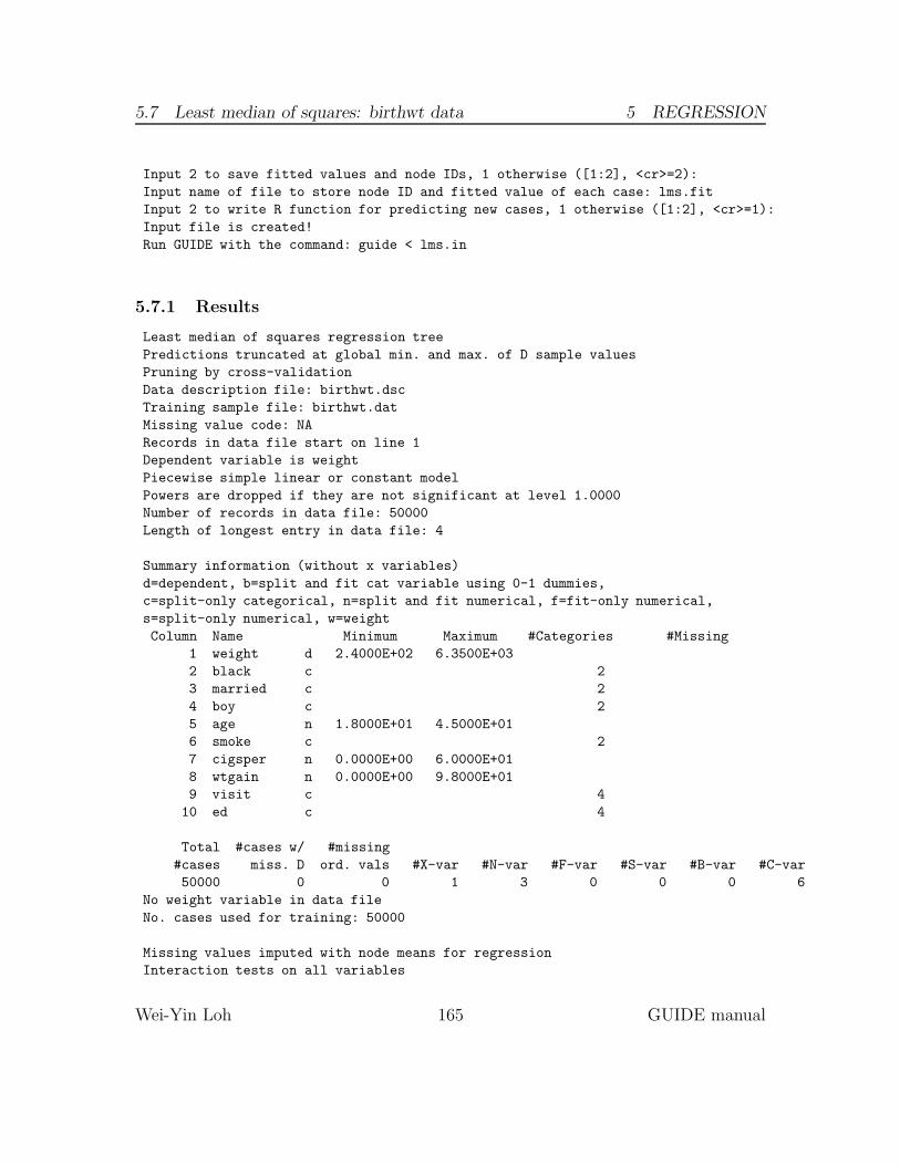
5.7 Least median of squares: birthwt data 5 REGRESSION
Input 2 to save fitted values and node IDs, 1 otherwise ([1:2], <cr>=2):
Input name of file to store node ID and fitted value of each case: lms.fit
Input 2 to write R function for predicting new cases, 1 otherwise ([1:2], <cr>=1):
Input file is created!
Run GUIDE with the command: guide < lms.in
5.7.1 Results
Least median of squares regression tree
Predictions truncated at global min. and max. of D sample values
Pruning by cross-validation
Data description file: birthwt.dsc
Training sample file: birthwt.dat
Missing value code: NA
Records in data file start on line 1
Dependent variable is weight
Piecewise simple linear or constant model
Powers are dropped if they are not significant at level 1.0000
Number of records in data file: 50000
Length of longest entry in data file: 4
Summary information (without x variables)
d=dependent, b=split and fit cat variable using 0-1 dummies,
c=split-only categorical, n=split and fit numerical, f=fit-only numerical,
s=split-only numerical, w=weight
Column Name Minimum Maximum #Categories #Missing
1 weight d 2.4000E+02 6.3500E+03
2 black c 2
3 married c 2
4 boy c 2
5 age n 1.8000E+01 4.5000E+01
6 smoke c 2
7 cigsper n 0.0000E+00 6.0000E+01
8 wtgain n 0.0000E+00 9.8000E+01
9 visit c 4
10 ed c 4
Total #cases w/ #missing
#cases miss. D ord. vals #X-var #N-var #F-var #S-var #B-var #C-var
50000 0 0 1 3 0 0 0 6
No weight variable in data file
No. cases used for training: 50000
Missing values imputed with node means for regression
Interaction tests on all variables
Wei-Yin Loh 165 GUIDE manual
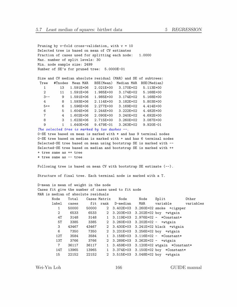
5.7 Least median of squares: birthwt data 5 REGRESSION
Pruning by v-fold cross-validation, with v = 10
Selected tree is based on mean of CV estimates
Fraction of cases used for splitting each node: 1.0000
Max. number of split levels: 30
Min. node sample size: 2499
Number of SE’s for pruned tree: 5.0000E-01
Size and CV median absolute residual (MAR) and SE of subtrees:
Tree #Tnodes Mean MAR BSE(Mean) Median MAR BSE(Median)
1 13 1.591E+06 2.021E+00 3.170E+02 5.113E+00
2 11 1.591E+06 1.985E+00 3.174E+02 5.168E+00
3-- 9 1.591E+06 1.985E+00 3.174E+02 5.168E+00
4 8 1.593E+06 2.114E+00 3.182E+02 5.803E+00
5++ 6 1.596E+06 2.277E+00 3.169E+02 4.414E+00
6 5 1.604E+06 2.244E+00 3.222E+02 4.482E+00
7 4 1.602E+06 2.090E+00 3.240E+02 4.692E+00
8 3 1.623E+06 2.715E+00 3.260E+02 3.087E+00
9 1 1.640E+06 9.479E-01 3.263E+02 9.920E-01
The selected tree is marked by two dashes --.
0-SE tree based on mean is marked with * and has 9 terminal nodes
0-SE tree based on median is marked with + and has 6 terminal nodes
Selected-SE tree based on mean using bootstrap SE is marked with --
Selected-SE tree based on median and bootstrap SE is marked with ++
+ tree same as ++ tree
* tree same as -- tree
Following tree is based on mean CV with bootstrap SE estimate (--).
Structure of final tree. Each terminal node is marked with a T.
D-mean is mean of weight in the node
Cases fit give the number of cases used to fit node
MAR is median of absolute residuals
Node Total Cases Matrix Node Node Split Other
label cases fit rank D-median MAR variable variables
1 50000 50000 2 3.402E+03 3.260E+02 smoke +cigsper
2 6533 6533 2 3.203E+03 3.202E+02 boy +wtgain
4T 3148 3148 1 3.119E+03 2.976E+02 - *Constant*
5T 3385 3385 2 3.260E+03 3.202E+02 - +wtgain
3 43467 43467 2 3.430E+03 3.241E+02 black +wtgain
6 7350 7350 2 3.231E+03 3.256E+02 boy +wtgain
12T 3584 3584 1 3.158E+03 3.116E+02 - *Constant*
13T 3766 3766 2 3.289E+03 3.262E+02 - +wtgain
7 36117 36117 1 3.459E+03 3.120E+02 wtgain *Constant*
14T 13965 13965 1 3.374E+03 3.150E+02 boy *Constant*
15 22152 22152 2 3.515E+03 3.048E+02 boy +wtgain
Wei-Yin Loh 166 GUIDE manual
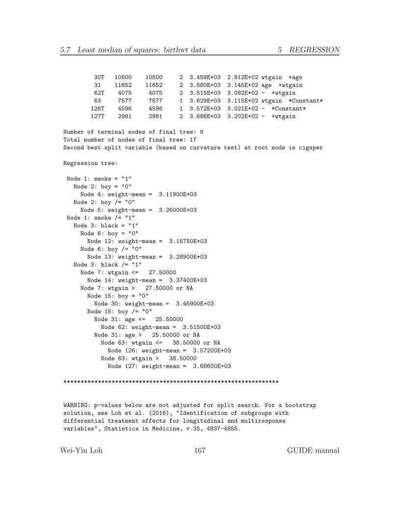
5.7 Least median of squares: birthwt data 5 REGRESSION
30T 10500 10500 2 3.459E+03 2.912E+02 wtgain +age
31 11652 11652 2 3.580E+03 3.145E+02 age +wtgain
62T 4075 4075 2 3.515E+03 3.082E+02 - +wtgain
63 7577 7577 1 3.629E+03 3.115E+02 wtgain *Constant*
126T 4596 4596 1 3.572E+03 3.021E+02 - *Constant*
127T 2981 2981 2 3.686E+03 3.202E+02 - +wtgain
Number of terminal nodes of final tree: 9
Total number of nodes of final tree: 17
Second best split variable (based on curvature test) at root node is cigsper
Regression tree:
Node 1: smoke = "1"
Node 2: boy = "0"
Node 4: weight-mean = 3.11900E+03
Node 2: boy /= "0"
Node 5: weight-mean = 3.26000E+03
Node 1: smoke /= "1"
Node 3: black = "1"
Node 6: boy = "0"
Node 12: weight-mean = 3.15750E+03
Node 6: boy /= "0"
Node 13: weight-mean = 3.28900E+03
Node 3: black /= "1"
Node 7: wtgain <= 27.50000
Node 14: weight-mean = 3.37400E+03
Node 7: wtgain > 27.50000 or NA
Node 15: boy = "0"
Node 30: weight-mean = 3.45900E+03
Node 15: boy /= "0"
Node 31: age <= 25.50000
Node 62: weight-mean = 3.51500E+03
Node 31: age > 25.50000 or NA
Node 63: wtgain <= 38.50000 or NA
Node 126: weight-mean = 3.57200E+03
Node 63: wtgain > 38.50000
Node 127: weight-mean = 3.68600E+03
***************************************************************
WARNING: p-values below are not adjusted for split search. For a bootstrap
solution, see Loh et al. (2016), "Identification of subgroups with
differential treatment effects for longitudinal and multiresponse
variables", Statistics in Medicine, v.35, 4837-4855.
Wei-Yin Loh 167 GUIDE manual

5.7 Least median of squares: birthwt data 5 REGRESSION
Node 1: Intermediate node
A case goes into Node 2 if smoke = "1"
smoke mode = "0"
Coefficients of least median of squares regression function:
Regressor Coefficient Minimum Mean Maximum
Constant 3.4160E+03
cigsper 7.8333E+00 0.00 1.4766 6.0000E+01
Mean of weight = 3402.0000000000000
Predicted values truncated at 240.00000000000000 & 6350.0000000000000
----------------------------
Node 2: Intermediate node
A case goes into Node 4 if boy = "0"
boy mode = "1"
----------------------------
Node 4: Terminal node
Coefficients of least median of squares regression function:
Regressor Coefficient Minimum Mean Maximum
Constant 3.1045E+03
cigsper 0.0000E+00 1.0011.1852 6.0000E+01
Mean of weight = 3119.0000000000000
Predicted values truncated at 240.00000000000000 & 6350.0000000000000
----------------------------
Node 5: Terminal node
Coefficients of least median of squares regression function:
Regressor Coefficient Minimum Mean Maximum
Constant 2.9496E+03
wtgain 1.0078E+01 0.0030.3412 9.8000E+01
Mean of weight = 3260.0000000000000
Predicted values truncated at 240.00000000000000 & 6350.0000000000000
----------------------------
Node 3: Intermediate node
A case goes into Node 6 if black = "1"
black mode = "0"
----------------------------
Node 6: Intermediate node
A case goes into Node 12 if boy = "0"
boy mode = "1"
----------------------------
Node 12: Terminal node
Coefficients of least median of squares regression function:
Regressor Coefficient Minimum Mean Maximum
Constant 3.2035E+03
wtgain 0.0000E+00 0.0028.9068 9.8000E+01
Mean of weight = 3157.5000000000000
Predicted values truncated at 240.00000000000000 & 6350.0000000000000
Wei-Yin Loh 168 GUIDE manual

5.7 Least median of squares: birthwt data 5 REGRESSION
----------------------------
Node 13: Terminal node
Coefficients of least median of squares regression function:
Regressor Coefficient Minimum Mean Maximum
Constant 3.1610E+03
wtgain 5.6500E+00 0.0029.7464 9.8000E+01
Mean of weight = 3289.0000000000000
Predicted values truncated at 240.00000000000000 & 6350.0000000000000
----------------------------
Node 7: Intermediate node
A case goes into Node 14 if wtgain <= 2.7500000E+01
wtgain mean = 3.1109E+01
----------------------------
Node 14: Terminal node
Coefficients of least median of squares regression function:
Regressor Coefficient Minimum Mean Maximum
Constant 3.3990E+03
age 0.0000E+00 18.0028.2233 4.5000E+01
Mean of weight = 3374.0000000000000
Predicted values truncated at 240.00000000000000 & 6350.0000000000000
----------------------------
Node 15: Intermediate node
A case goes into Node 30 if boy = "0"
boy mode = "1"
----------------------------
Node 30: Terminal node
Coefficients of least median of squares regression function:
Regressor Coefficient Minimum Mean Maximum
Constant 3.0386E+03
age 1.4250E+01 18.0027.8578 4.5000E+01
Mean of weight = 3459.0000000000000
Predicted values truncated at 240.00000000000000 & 6350.0000000000000
----------------------------
Node 31: Intermediate node
A case goes into Node 62 if age <= 2.5500000E+01
age mean = 2.7833E+01
----------------------------
Node 62: Terminal node
Coefficients of least median of squares regression function:
Regressor Coefficient Minimum Mean Maximum
Constant 3.2105E+03
wtgain 8.5000E+00 28.0039.8321 9.8000E+01
Mean of weight = 3515.0000000000000
Predicted values truncated at 240.00000000000000 & 6350.0000000000000
----------------------------
Node 63: Intermediate node
Wei-Yin Loh 169 GUIDE manual

5.8 Poisson regression with offset: lung cancer data 5 REGRESSION
A case goes into Node 126 if wtgain <= 3.8500000E+01 or NA
wtgain mean = 3.7770E+01
----------------------------
Node 126: Terminal node
Coefficients of least median of squares regression function:
Regressor Coefficient Minimum Mean Maximum
Constant 3.5820E+03
wtgain 0.0000E+00 28.0032.3040 3.8000E+01
Mean of weight = 3572.0000000000000
Predicted values truncated at 240.00000000000000 & 6350.0000000000000
----------------------------
Node 127: Terminal node
Coefficients of least median of squares regression function:
Regressor Coefficient Minimum Mean Maximum
Constant 3.3170E+03
wtgain 8.0000E+00 39.0046.1962 9.8000E+01
Mean of weight = 3686.0000000000000
Predicted values truncated at 240.00000000000000 & 6350.0000000000000
----------------------------
Proportion of deviance explained by tree model: .0735
Observed and fitted values are stored in lms.fit
LaTeX code for tree is in lms.tex
The tree is shown in Figure 16.
5.8 Poisson regression with offset: lung cancer data
We use a data set from an epidemiological study of the effect of public drinking wateron cancer mortality in Missouri (Choi et al., 2005). Our data file lungcancer.txtgives the number of deaths (deaths) from lung cancer among 115 counties (county)during the period 1972–1981 for both sexes (sex) and four age groups (agegp): 45–54, 55–64, 65–74, and over 75. The description file lungcancer.dsc below liststhe variables together with the county population (pop) and the natural log of pop(logpop). The latter is specified as z to serve an an offset variable and the formeris excluded (x) from the analysis. For the purpose of illustration, we specify sex asb to allow its dummy indicator variable to serve as a linear predictor in the nodePoisson models. The contents of lungcancer.dsc are:
lungcancer.txt
NA
1
1 county c
2 sex b
Wei-Yin Loh 170 GUIDE manual

5.8 Poisson regression with offset: lung cancer data 5 REGRESSION
smoke= 1 1
boy= 0 2
4
3148
3119.
5
33853260.
+wtgain
black= 1 3
boy= 0 6
12
3584
3158.
13
3766
3289.+wtgain
wtgain≤ 27.50 7
14
139653374.
boy= 0 15
30
105003459.+age
age≤ 25.50 31
62
4075
3515.+wtgain
wtgain≤∗38.50 63
126
4596
3572.
127
29813686.
+wtgain
Figure 16: GUIDE v.27.9 0.50-SE piecewise simple linear least-median-of-squaresregression tree for predicting weight. Maximum number of split levels is 30 andminimum node sample size is 2499. At each split, an observation goes to the leftbranch if and only if the condition is satisfied. The symbol ‘≤∗’ stands for ‘≤ ormissing’. Sample size (in italics), mean of weight, and sign and name of regressorvariables printed below nodes. Nodes with negative and positive slopes are coloredred and green, respectively. Second best split variable at root node is cigsper.
Wei-Yin Loh 171 GUIDE manual

5.8 Poisson regression with offset: lung cancer data 5 REGRESSION
3 agegp c
4 deaths d
5 pop x
6 logpop z
Our goal is to construct a Poisson regression tree for the gender-specific rate of lungcancer deaths, where rate is the expected number of deaths in a county divided byits population size for each gender. That is, letting µ denote the expected numberof gender-specific deaths in a county, we fit this model in each node of the tree:
log(µ/pop) = β0 + β1I(sex = M)
or, equivalently,log(µ) = β0 + β1I(sex = M) + logpop.
5.8.1 Input file creation
0. Read the warranty disclaimer
1. Create a GUIDE input file
Input your choice: 1
Name of batch input file: poi.in
Input 1 for model fitting, 2 for importance or DIF scoring,
3 for data conversion ([1:3], <cr>=1):
Name of batch output file: poi.out
Input 1 for single tree, 2 for ensemble ([1:2], <cr>=1):
Input 1 for classification, 2 for regression, 3 for propensity score grouping
(propensity score grouping is an experimental option)
Input your choice ([1:3], <cr>=1): 2
Choose type of regression model:
1=linear, 2=quantile, 3=Poisson, 4=proportional hazards,
5=multiresponse or itemresponse, 6=longitudinal data (with T variables).
Input choice ([1:6], <cr>=1): 3
Choose Poisson regression here.
Choose complexity of model to use at each node:
Choose 1 for multiple regression (recommended if R variable is present,
unless there are too many N, F or B variables)
Choose 2 for best polynomial in one N or F variable + R (if present)
Choose 3 to fit a constant + R (if present)
1: multiple linear, 2: best polynomial, 3: constant ([1:3], <cr>=1):
Input 1 for default options, 2 otherwise ([1:2], <cr>=1):
Input name of data description file (max 100 characters);
enclose with matching quotes if it has spaces: lungcancer.dsc
Wei-Yin Loh 172 GUIDE manual

5.8 Poisson regression with offset: lung cancer data 5 REGRESSION
Reading data description file ...
Training sample file: lungcancer.txt
Missing value code: NA
Records in data file start on line 1
Dependent variable is deaths
Reading data file ...
Number of records in data file: 920
Length of longest entry in data file: 8
Checking for missing values ...
Total number of cases: 920
Col. no. Categorical variable #levels #missing values
1 county 115 0
2 sex 2 0
3 agegp 4 0
Re-checking data ...
Assigning codes to categorical and missing values
Data checks complete
Number of cases with positive D values: 869
GUIDE will try to create the variables in the description file.
If it is unsuccessful, please create the columns yourself...
Number of dummy variables created: 1
Creating dummy variables
Rereading data
Total #cases w/ #missing
#cases miss. D ord. vals #X-var #N-var #F-var #S-var #B-var #C-var
920 0 0 1 0 0 0 1 2
Offset variable in column: 6
No. cases used for training: 920
Finished reading data file
Input 1 for LaTeX tree code, 2 to skip it ([1:2], <cr>=1):
Input file name to store LaTeX code (use .tex as suffix): poi.tex
Input 2 to save fitted values and node IDs, 1 otherwise ([1:2], <cr>=2):
Input name of file to store node ID and fitted value of each case: poi.fit
Input 2 to write R function for predicting new cases, 1 otherwise ([1:2], <cr>=1):
Input file is created!
Run GUIDE with the command: guide < poi.in
5.8.2 Results
Poisson regression tree
No truncation of predicted values
Pruning by cross-validation
Data description file: lungcancer.dsc
Training sample file: lungcancer.txt
Missing value code: NA
Wei-Yin Loh 173 GUIDE manual
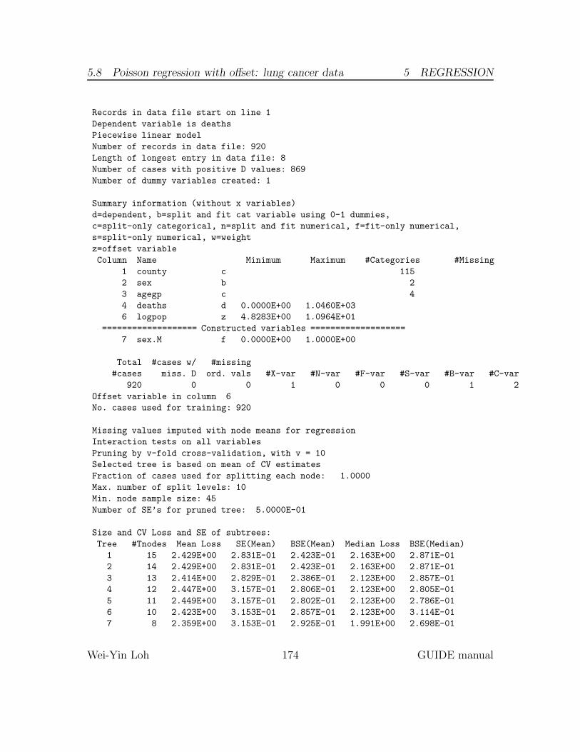
5.8 Poisson regression with offset: lung cancer data 5 REGRESSION
Records in data file start on line 1
Dependent variable is deaths
Piecewise linear model
Number of records in data file: 920
Length of longest entry in data file: 8
Number of cases with positive D values: 869
Number of dummy variables created: 1
Summary information (without x variables)
d=dependent, b=split and fit cat variable using 0-1 dummies,
c=split-only categorical, n=split and fit numerical, f=fit-only numerical,
s=split-only numerical, w=weight
z=offset variable
Column Name Minimum Maximum #Categories #Missing
1 county c 115
2 sex b 2
3 agegp c 4
4 deaths d 0.0000E+00 1.0460E+03
6 logpop z 4.8283E+00 1.0964E+01
=================== Constructed variables ===================
7 sex.M f 0.0000E+00 1.0000E+00
Total #cases w/ #missing
#cases miss. D ord. vals #X-var #N-var #F-var #S-var #B-var #C-var
920 0 0 1 0 0 0 1 2
Offset variable in column 6
No. cases used for training: 920
Missing values imputed with node means for regression
Interaction tests on all variables
Pruning by v-fold cross-validation, with v = 10
Selected tree is based on mean of CV estimates
Fraction of cases used for splitting each node: 1.0000
Max. number of split levels: 10
Min. node sample size: 45
Number of SE’s for pruned tree: 5.0000E-01
Size and CV Loss and SE of subtrees:
Tree #Tnodes Mean Loss SE(Mean) BSE(Mean) Median Loss BSE(Median)
1 15 2.429E+00 2.831E-01 2.423E-01 2.163E+00 2.871E-01
2 14 2.429E+00 2.831E-01 2.423E-01 2.163E+00 2.871E-01
3 13 2.414E+00 2.829E-01 2.386E-01 2.123E+00 2.857E-01
4 12 2.447E+00 3.157E-01 2.806E-01 2.123E+00 2.805E-01
5 11 2.449E+00 3.157E-01 2.802E-01 2.123E+00 2.786E-01
6 10 2.423E+00 3.153E-01 2.857E-01 2.123E+00 3.114E-01
7 8 2.359E+00 3.153E-01 2.925E-01 1.991E+00 2.698E-01
Wei-Yin Loh 174 GUIDE manual

5.8 Poisson regression with offset: lung cancer data 5 REGRESSION
8 7 2.424E+00 3.563E-01 3.029E-01 1.991E+00 3.756E-01
9 4 2.455E+00 3.772E-01 3.185E-01 1.925E+00 4.297E-01
10** 3 2.318E+00 3.595E-01 3.111E-01 1.709E+00 5.118E-01
11 2 4.857E+00 8.176E-01 5.168E-01 4.388E+00 7.094E-01
12 1 9.439E+00 1.406E+00 1.131E+00 9.048E+00 1.683E+00
0-SE tree based on mean is marked with * and has 3 terminal nodes
0-SE tree based on median is marked with + and has 3 terminal nodes
Selected-SE tree based on mean using naive SE is marked with **
Selected-SE tree based on mean using bootstrap SE is marked with --
Selected-SE tree based on median and bootstrap SE is marked with ++
** tree and ++ tree are the same
Following tree is based on mean CV with naive SE estimate (**).
Structure of final tree. Each terminal node is marked with a T.
Rate is mean of Y/exp(offset)
Cases fit give the number of cases used to fit node
Deviance is mean residual deviance for all cases in node
Node Total Cases Matrix Node Node Split Other
label cases fit rank rate deviance variable variables
1 920 920 2 1.382E-02 9.179E+00 agegp
2T 230 230 2 5.493E-03 1.863E+00 county
3 690 690 2 1.763E-02 4.357E+00 agegp
6T 230 230 2 1.339E-02 3.003E+00 county
7T 460 460 2 2.093E-02 1.802E+00 agegp
Number of terminal nodes of final tree: 3
Total number of nodes of final tree: 5
Second best split variable (based on curvature test) at root node is sex
Regression tree:
Node 1: agegp = "45-54"
Node 2: deaths sample rate = 5.49286E-03
Node 1: agegp /= "45-54"
Node 3: agegp = "55-64"
Node 6: deaths sample rate = 1.33898E-02
Node 3: agegp /= "55-64"
Node 7: deaths sample rate = 2.09327E-02
***************************************************************
WARNING: p-values below are not adjusted for split search. For a bootstrap
Wei-Yin Loh 175 GUIDE manual

5.8 Poisson regression with offset: lung cancer data 5 REGRESSION
solution, see Loh et al. (2016), "Identification of subgroups with
differential treatment effects for longitudinal and multiresponse
variables", Statistics in Medicine, v.35, 4837-4855.
Node 1: Intermediate node
A case goes into Node 2 if agegp = "45-54"
agegp mode = "45-54"
Coefficients of loglinear regression function:
Regressor Coefficient t-stat p-val Minimum Mean Maximum
Constant -5.1717E+00 -366.86 0.0000
sex.M 1.4370E+00 89.64 0.0000 0.0000E+00 5.0000E-01 1.0000E+00
Node mean for offset variable = 6.7275E+00
----------------------------
Node 2: Terminal node
Coefficients of loglinear regression function:
Regressor Coefficient t-stat p-val Minimum Mean Maximum
Constant -5.8337E+00 -161.46 0.0000
sex.M 1.0384E+00 24.44 0.0000 0.0000E+00 5.0000E-01 1.0000E+00
Node mean for offset variable = 6.8567E+00
----------------------------
Node 3: Intermediate node
A case goes into Node 6 if agegp = "55-64"
agegp mode = "55-64"
----------------------------
Node 6: Terminal node
Coefficients of loglinear regression function:
Regressor Coefficient t-stat p-val Minimum Mean Maximum
Constant -5.1175E+00 -199.84 0.0000
sex.M 1.2854E+00 43.87 0.0000 0.0000E+00 5.0000E-01 1.0000E+00
Node mean for offset variable = 6.9199E+00
----------------------------
Node 7: Terminal node
Coefficients of loglinear regression function:
Regressor Coefficient t-stat p-val Minimum Mean Maximum
Constant -4.9065E+00 -256.88 0.0000
sex.M 1.7137E+00 79.68 0.0000 0.0000E+00 5.0000E-01 1.0000E+00
Node mean for offset variable = 6.5666E+00
----------------------------
Observed and fitted values are stored in poi.fit
LaTeX code for tree is in poi.tex
The results show that the death rate increases with age and that the rate formales is consistently higher than that for females. The tree diagram is given inFigure 17.
Wei-Yin Loh 176 GUIDE manual
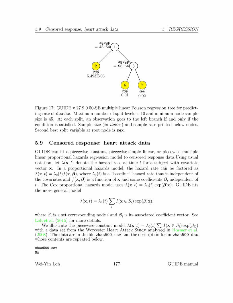
5.9 Censored response: heart attack data 5 REGRESSION
agegp= 45-54 1
2
2305.493E-03
agegp= 55-64 3
6
2300.01
7
460
0.02
Figure 17: GUIDE v.27.9 0.50-SE multiple linear Poisson regression tree for predict-ing rate of deaths. Maximum number of split levels is 10 and minimum node samplesize is 45. At each split, an observation goes to the left branch if and only if thecondition is satisfied. Sample size (in italics) and sample rate printed below nodes.Second best split variable at root node is sex.
5.9 Censored response: heart attack data
GUIDE can fit a piecewise-constant, piecewise-simple linear, or piecewise multiplelinear proportional hazards regression model to censored response data.Using usualnotation, let λ(x, t) denote the hazard rate at time t for a subject with covariatevector x. In a proportional hazards model, the hazard rate can be factored asλ(x, t) = λ0(t)f(x,β), where λ0(t) is a “baseline” hazard rate that is independent ofthe covariates and f(x,β) is a function of x and some coefficients β, independent oft. The Cox proportional hazards model uses λ(x, t) = λ0(t) exp(β
′x). GUIDE fitsthe more general model
λ(x, t) = λ0(t)∑
i
I(x ∈ Si) exp(β′ix),
where Si is a set corresponding node i and βi is its associated coefficient vector. SeeLoh et al. (2015) for more details.
We illustrate the piecewise-constant model λ(x, t) = λ0(t)∑
i I(x ∈ Si) exp(βi0)with a data set from the Worcester Heart Attack Study analyzed in Hosmer et al.(2008). The data are in the file whas500.csv and the description file in whas500.dscwhose contents are repeated below.
whas500.csv
NA
Wei-Yin Loh 177 GUIDE manual

5.9 Censored response: heart attack data 5 REGRESSION
1
1 id x
2 age n
3 gender c
4 hr n
5 sysbp n
6 diasbp n
7 bmi n
8 cvd c
9 afb c
10 sho c
11 chf c
12 av3 c
13 miord c
14 mitype c
15 year c
16 admitdate x
17 disdate x
18 fdate x
19 los n
20 dstat x
21 lenfol t
22 fstat d
The goal of the study is to observe survival rates following hospital admission foracute myocardial infarction. The response variable is lenfol, which stands for totallength of follow-up in days. Variable fstat is status at last follow-up (0=alive,1=dead) and variable chf is congestive heart complications (0=no, 1=yes).
0. Read the warranty disclaimer
1. Create a GUIDE input file
Input your choice: 1
Name of batch input file: whas500.in
Input 1 for model fitting, 2 for importance or DIF scoring,
3 for data conversion ([1:3], <cr>=1):
Name of batch output file: whas500.out
Input 1 for single tree, 2 for ensemble ([1:2], <cr>=1):
Input 1 for classification, 2 for regression, 3 for propensity score grouping
(propensity score grouping is an experimental option)
Input your choice ([1:3], <cr>=1): 2
Choose type of regression model:
1=linear, 2=quantile, 3=Poisson, 4=proportional hazards,
5=multiresponse or itemresponse, 6=longitudinal data (with T variables).
Input choice ([1:6], <cr>=1): 4
Choose complexity of model to use at each node:
Choose 1 for multiple regression (recommended if R variable is present,
Wei-Yin Loh 178 GUIDE manual

5.9 Censored response: heart attack data 5 REGRESSION
unless there are too many N, F or B variables)
Choose 2 for best polynomial in one N or F variable + R (if present)
Choose 3 to fit a constant + R (if present)
1: multiple linear, 2: best polynomial, 3: constant ([1:3], <cr>=3):
Input 1 for default options, 2 otherwise ([1:2], <cr>=1):
Input name of data description file (max 100 characters);
enclose with matching quotes if it has spaces: whas500.dsc
Reading data description file ...
Training sample file: whas500.csv
Missing value code: NA
Records in data file start on line 1
Warning: N variables changed to S
Dependent variable is fstat
Reading data file ...
Number of records in data file: 500
Length of longest entry in data file: 10
Checking for missing values ...
Total number of cases: 500
Col. no. Categorical variable #levels #missing values
3 gender 2 0
8 cvd 2 0
9 afb 2 0
10 sho 2 0
11 chf 2 0
12 av3 2 0
13 miord 2 0
14 mitype 2 0
15 year 3 0
Re-checking data ...
Assigning codes to categorical and missing values
Data checks complete
Smallest uncensored T: 1.0000
No. complete cases excluding censored T < smallest uncensored T: 500
No. cases used to compute baseline hazard: 500
No. cases with D=1 and T >= smallest uncensored: 215
Rereading data
Total #cases w/ #missing
#cases miss. D ord. vals #X-var #N-var #F-var #S-var #B-var #C-var
500 0 0 5 0 0 6 0 9
Survival time variable in column: 21
Event indicator variable in column: 22
Proportion uncensored among nonmissing T and D variables: .430
No. cases used for training: 500
Finished reading data file
Input 1 for LaTeX tree code, 2 to skip it ([1:2], <cr>=1):
Wei-Yin Loh 179 GUIDE manual

5.9 Censored response: heart attack data 5 REGRESSION
Input file name to store LaTeX code (use .tex as suffix): whas500.tex
Input 2 to save fitted values and node IDs, 1 otherwise ([1:2], <cr>=2):
Input name of file to store node ID and fitted value of each case: whas500.fit
Input 2 to write R function for predicting new cases, 1 otherwise ([1:2], <cr>=1):
Input file is created!
Run GUIDE with the command: guide < whas500.in
5.9.1 Results
Proportional hazards regression with relative risk estimates
Pruning by cross-validation
Data description file: whas500.dsc
Training sample file: whas500.csv
Missing value code: NA
Records in data file start on line 1
Warning: N variables changed to S
Dependent variable is fstat
Piecewise constant model
Number of records in data file: 500
Length of longest entry in data file: 10
Smallest uncensored T: 1.0000
No. complete cases excluding censored T < smallest uncensored T: 500
No. cases used to compute baseline hazard: 500
No. cases with D=1 and T >= smallest uncensored: 215
Summary information (without x variables)
d=dependent, b=split and fit cat variable using 0-1 dummies,
c=split-only categorical, n=split and fit numerical, f=fit-only numerical,
s=split-only numerical, w=weight
t=survival time variable
Column Name Minimum Maximum #Categories #Missing
2 age s 3.0000E+01 1.0400E+02
3 gender c 2
4 hr s 3.5000E+01 1.8600E+02
5 sysbp s 5.7000E+01 2.4400E+02
6 diasbp s 6.0000E+00 1.9800E+02
7 bmi s 1.3045E+01 4.4839E+01
8 cvd c 2
9 afb c 2
10 sho c 2
11 chf c 2
12 av3 c 2
13 miord c 2
14 mitype c 2
15 year c 3
19 los s 0.0000E+00 4.7000E+01
Wei-Yin Loh 180 GUIDE manual
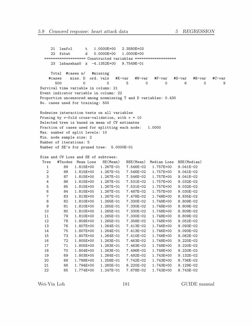
5.9 Censored response: heart attack data 5 REGRESSION
21 lenfol t 1.0000E+00 2.3580E+03
22 fstat d 0.0000E+00 1.0000E+00
=================== Constructed variables ===================
23 lnbasehaz0 z -4.1352E+00 9.7549E-01
Total #cases w/ #missing
#cases miss. D ord. vals #X-var #N-var #F-var #S-var #B-var #C-var
500 0 0 5 0 0 6 0 9
Survival time variable in column: 21
Event indicator variable in column: 22
Proportion uncensored among nonmissing T and D variables: 0.430
No. cases used for training: 500
Nodewise interaction tests on all variables
Pruning by v-fold cross-validation, with v = 10
Selected tree is based on mean of CV estimates
Fraction of cases used for splitting each node: 1.0000
Max. number of split levels: 10
Min. node sample size: 2
Number of iterations: 5
Number of SE’s for pruned tree: 5.0000E-01
Size and CV Loss and SE of subtrees:
Tree #Tnodes Mean Loss SE(Mean) BSE(Mean) Median Loss BSE(Median)
1 89 1.815E+00 1.267E-01 7.546E-02 1.757E+00 9.041E-02
2 88 1.815E+00 1.267E-01 7.546E-02 1.757E+00 9.041E-02
3 87 1.815E+00 1.267E-01 7.546E-02 1.757E+00 9.041E-02
4 86 1.815E+00 1.267E-01 7.531E-02 1.757E+00 9.032E-02
5 85 1.815E+00 1.267E-01 7.531E-02 1.757E+00 9.032E-02
6 84 1.815E+00 1.267E-01 7.487E-02 1.757E+00 9.030E-02
7 83 1.813E+00 1.267E-01 7.478E-02 1.748E+00 8.835E-02
8 82 1.810E+00 1.265E-01 7.330E-02 1.748E+00 8.809E-02
9 81 1.810E+00 1.265E-01 7.330E-02 1.748E+00 8.809E-02
10 80 1.810E+00 1.265E-01 7.330E-02 1.748E+00 8.809E-02
11 79 1.810E+00 1.265E-01 7.330E-02 1.748E+00 8.809E-02
12 78 1.809E+00 1.265E-01 7.358E-02 1.748E+00 9.052E-02
13 76 1.807E+00 1.264E-01 7.413E-02 1.746E+00 9.093E-02
14 75 1.807E+00 1.264E-01 7.413E-02 1.746E+00 9.093E-02
15 73 1.807E+00 1.264E-01 7.410E-02 1.748E+00 9.062E-02
16 72 1.805E+00 1.263E-01 7.463E-02 1.748E+00 9.220E-02
17 71 1.805E+00 1.263E-01 7.463E-02 1.748E+00 9.220E-02
18 70 1.804E+00 1.263E-01 7.496E-02 1.748E+00 9.220E-02
19 69 1.803E+00 1.264E-01 7.492E-02 1.743E+00 9.132E-02
20 68 1.788E+00 1.258E-01 7.742E-02 1.743E+00 8.736E-02
21 66 1.794E+00 1.260E-01 8.220E-02 1.743E+00 9.129E-02
22 65 1.774E+00 1.247E-01 7.678E-02 1.743E+00 8.743E-02
Wei-Yin Loh 181 GUIDE manual

5.9 Censored response: heart attack data 5 REGRESSION
23 63 1.767E+00 1.250E-01 7.489E-02 1.743E+00 8.114E-02
24 62 1.762E+00 1.225E-01 7.662E-02 1.743E+00 9.097E-02
25 61 1.759E+00 1.226E-01 7.607E-02 1.732E+00 8.777E-02
26 60 1.745E+00 1.217E-01 7.985E-02 1.732E+00 8.188E-02
27 57 1.710E+00 1.173E-01 5.366E-02 1.732E+00 7.992E-02
28 56 1.710E+00 1.173E-01 5.366E-02 1.732E+00 7.992E-02
29 54 1.711E+00 1.172E-01 5.375E-02 1.732E+00 8.126E-02
30 52 1.709E+00 1.172E-01 5.254E-02 1.732E+00 8.248E-02
31 51 1.706E+00 1.173E-01 5.087E-02 1.732E+00 8.240E-02
32 42 1.692E+00 1.154E-01 5.402E-02 1.732E+00 9.936E-02
33 39 1.684E+00 1.148E-01 5.327E-02 1.691E+00 9.347E-02
34 38 1.681E+00 1.148E-01 5.449E-02 1.688E+00 9.546E-02
35 37 1.626E+00 1.116E-01 5.622E-02 1.607E+00 9.510E-02
36 36 1.619E+00 1.114E-01 5.900E-02 1.567E+00 9.905E-02
37 34 1.619E+00 1.113E-01 5.881E-02 1.567E+00 9.753E-02
38 31 1.597E+00 1.106E-01 5.094E-02 1.532E+00 8.824E-02
39 29 1.589E+00 1.099E-01 5.172E-02 1.534E+00 7.898E-02
40 28 1.567E+00 1.091E-01 5.671E-02 1.503E+00 8.495E-02
41 26 1.528E+00 1.059E-01 6.938E-02 1.489E+00 1.034E-01
42 25 1.525E+00 1.052E-01 7.119E-02 1.457E+00 1.023E-01
43 22 1.511E+00 1.042E-01 7.765E-02 1.457E+00 1.048E-01
44 19 1.475E+00 1.020E-01 7.820E-02 1.432E+00 1.128E-01
45 18 1.433E+00 9.776E-02 7.466E-02 1.426E+00 1.044E-01
46 17 1.413E+00 9.672E-02 7.751E-02 1.426E+00 1.245E-01
47 16 1.397E+00 9.612E-02 7.667E-02 1.392E+00 1.056E-01
48 12 1.393E+00 9.598E-02 7.846E-02 1.386E+00 1.024E-01
49* 8 1.220E+00 7.499E-02 3.670E-02 1.253E+00 5.366E-02
50++ 6 1.220E+00 7.158E-02 3.824E-02 1.204E+00 5.526E-02
51** 5 1.243E+00 7.171E-02 3.991E-02 1.263E+00 5.840E-02
52 4 1.281E+00 7.154E-02 4.064E-02 1.270E+00 4.950E-02
53 3 1.300E+00 7.015E-02 3.646E-02 1.319E+00 3.915E-02
54 2 1.325E+00 6.506E-02 2.839E-02 1.313E+00 3.556E-02
55 1 1.503E+00 5.698E-02 2.544E-02 1.484E+00 3.699E-02
0-SE tree based on mean is marked with * and has 8 terminal nodes
0-SE tree based on median is marked with + and has 6 terminal nodes
Selected-SE tree based on mean using naive SE is marked with **
Selected-SE tree based on mean using bootstrap SE is marked with --
Selected-SE tree based on median and bootstrap SE is marked with ++
++ tree same as -- tree
+ tree same as ++ tree
Following tree is based on mean CV with naive SE estimate (**).
Structure of final tree. Each terminal node is marked with a T.
Wei-Yin Loh 182 GUIDE manual
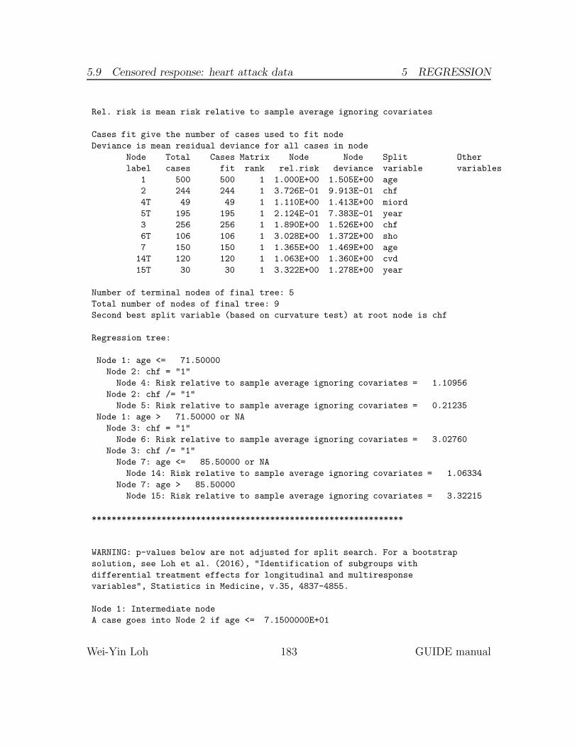
5.9 Censored response: heart attack data 5 REGRESSION
Rel. risk is mean risk relative to sample average ignoring covariates
Cases fit give the number of cases used to fit node
Deviance is mean residual deviance for all cases in node
Node Total Cases Matrix Node Node Split Other
label cases fit rank rel.risk deviance variable variables
1 500 500 1 1.000E+00 1.505E+00 age
2 244 244 1 3.726E-01 9.913E-01 chf
4T 49 49 1 1.110E+00 1.413E+00 miord
5T 195 195 1 2.124E-01 7.383E-01 year
3 256 256 1 1.890E+00 1.526E+00 chf
6T 106 106 1 3.028E+00 1.372E+00 sho
7 150 150 1 1.365E+00 1.469E+00 age
14T 120 120 1 1.063E+00 1.360E+00 cvd
15T 30 30 1 3.322E+00 1.278E+00 year
Number of terminal nodes of final tree: 5
Total number of nodes of final tree: 9
Second best split variable (based on curvature test) at root node is chf
Regression tree:
Node 1: age <= 71.50000
Node 2: chf = "1"
Node 4: Risk relative to sample average ignoring covariates = 1.10956
Node 2: chf /= "1"
Node 5: Risk relative to sample average ignoring covariates = 0.21235
Node 1: age > 71.50000 or NA
Node 3: chf = "1"
Node 6: Risk relative to sample average ignoring covariates = 3.02760
Node 3: chf /= "1"
Node 7: age <= 85.50000 or NA
Node 14: Risk relative to sample average ignoring covariates = 1.06334
Node 7: age > 85.50000
Node 15: Risk relative to sample average ignoring covariates = 3.32215
***************************************************************
WARNING: p-values below are not adjusted for split search. For a bootstrap
solution, see Loh et al. (2016), "Identification of subgroups with
differential treatment effects for longitudinal and multiresponse
variables", Statistics in Medicine, v.35, 4837-4855.
Node 1: Intermediate node
A case goes into Node 2 if age <= 7.1500000E+01
Wei-Yin Loh 183 GUIDE manual

5.9 Censored response: heart attack data 5 REGRESSION
age mean = 6.9846E+01
Coefficients of log-relative risk function:
Regressor Coefficient t-stat p-val
Constant -3.5381E-02
Predicted relative risk = 1.0000000000000000
----------------------------
Node 2: Intermediate node
A case goes into Node 4 if chf = "1"
chf mode = "0"
----------------------------
Node 4: Terminal node
Coefficients of log-relative risk function:
Regressor Coefficient t-stat p-val
Constant 6.8580E-02
Predicted relative risk = 1.1095574995429367
----------------------------
Node 5: Terminal node
Coefficients of log-relative risk function:
Regressor Coefficient t-stat p-val
Constant -1.5849E+00
Predicted relative risk = 0.21235168812700622
----------------------------
Node 3: Intermediate node
A case goes into Node 6 if chf = "1"
chf mode = "0"
----------------------------
Node 6: Terminal node
Coefficients of log-relative risk function:
Regressor Coefficient t-stat p-val
Constant 1.0724E+00
Predicted relative risk = 3.0276015801608627
----------------------------
Node 7: Intermediate node
A case goes into Node 14 if age <= 8.5500000E+01 or NA
age mean = 8.0667E+01
----------------------------
Node 14: Terminal node
Coefficients of log-relative risk function:
Regressor Coefficient t-stat p-val
Constant 2.6029E-02
Predicted relative risk = 1.0633351387096228
----------------------------
Node 15: Terminal node
Coefficients of log-relative risk function:
Regressor Coefficient t-stat p-val
Constant 1.1652E+00
Wei-Yin Loh 184 GUIDE manual

5.9 Censored response: heart attack data 5 REGRESSION
age≤ 71.50 1
chf= 1 2
4
491.11
5
1950.21
chf= 1 3
6
1063.03
age≤∗85.50 7
14
1201.06
15
303.32
Figure 18: GUIDE v.27.9 0.50-SE piecewise constant relative risk regression treefor predicting fstat. Maximum number of split levels is 10 and minimum nodesample size is 2. At each split, an observation goes to the left branch if and only ifthe condition is satisfied. The symbol ‘≤∗’ stands for ‘≤ or missing’. Sample size(in italics) and mean relative risks (relative to sample average ignoring covariates)printed below nodes. Second best split variable at root node is chf.
Predicted relative risk = 3.3221527399879980
----------------------------
Observed and fitted values are stored in whas500.fit
LaTeX code for tree is in whas500.tex
The tree model, given in Figure 18, shows that risk of death is lowest (0.21relative to the sample average for the whole data set) for those younger than 72 withno congestive heart complications. The groups with the highest risks (3.03–3.32relative to average) are those older than 71 with congestive heart complications andthose older than 85 without congestive heart complications.
The top few lines of the file whas500.fit and its column definitions are:
train node survivaltime logbasecumhaz relativerisk survivalprob mediansurvtime
y 14 2.178000E+03 -7.667985E-02 1.063335E+00 3.865048E-01 1.553833E+03
y 5 2.172000E+03 -7.667985E-02 2.123517E-01 8.270912E-01 2.354277E+03
y 5 2.190000E+03 -7.667985E-02 2.123517E-01 8.270912E-01 2.354277E+03
y 4 2.970000E+02 -1.320296E+00 1.109557E+00 7.512523E-01 1.534963E+03
Wei-Yin Loh 185 GUIDE manual

5.10 Multi-response: public health data 5 REGRESSION
The columns are:
train: “y” if the observation is used for model fitting, “n” if not.
node: terminal node label of observation.
survivaltime: observed survival time t.
logbasecumhaz: log of the estimated baseline cumulative hazard function log Λ0(t) =log
∫ t
0λ0(u) du at observed time t.
relativerisk: exp(β′x − β∗), risk of death relative to the average for the sample,where x is the covariate vector of the observation, β is the estimated regressioncoefficient vector in the node, and β∗ is the coefficient in the constant modelλ0(t) exp(β∗) fitted to all the training cases in the root node. Because a constantis fitted to each node here, β∗ = −0.035381 is the value of β at the root node.For example, the first subject, which is in node 14, has β = 0.026029 and sorelativerisk = exp(β − β∗) = exp(0.026029 + 0.035381) = 1.063335.
survivalprob: probability that the subject survives up to observed time t. For thefirst subject, this is
exp{−Λ0(t) exp(β′x)} = exp{− exp(β∗ + logbasecumhaz)× relativerisk}
= exp(− exp(−0.035381− 0.07667985)× 1.063335)
= 0.3865049.
mediansurvtime: estimated median survival time t such that exp{−Λ0(t) exp(β′x)} =
0.5, or, equivalently, Λ0(t) exp(β′ix) = − log(0.5), or logbasecumhaz(t) =
log log(2) − β′ix, using linear interpolation of Λ0(t). Median survival times
greater than the largest observed time have a trailing plus (+) sign.
5.10 Multi-response: public health data
GUIDE can fit a piecewise-constant regression model for two or more dependentvariables simultaneously (Loh and Zheng, 2013). We demonstrate this with the dataset phs.dat from a public health survey of about 120,000 respondents. There arethree D variables, namely, total restricted activity days in the past 2 week (raday),number of doctor visits in the past 12 months (visit), and number of short-stayhospital days in the past 12 months (hda12). The description files phs.dsc givenbelow lists 6 numeric and 9 categorical variables.
Wei-Yin Loh 186 GUIDE manual
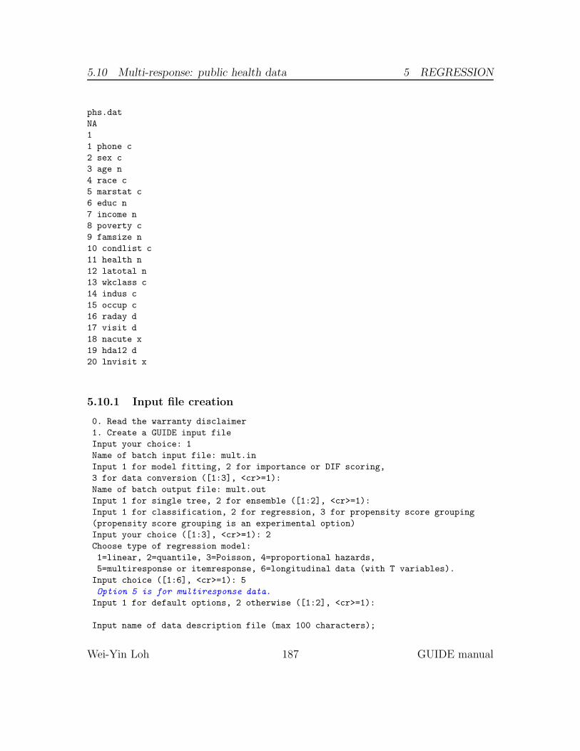
5.10 Multi-response: public health data 5 REGRESSION
phs.dat
NA
1
1 phone c
2 sex c
3 age n
4 race c
5 marstat c
6 educ n
7 income n
8 poverty c
9 famsize n
10 condlist c
11 health n
12 latotal n
13 wkclass c
14 indus c
15 occup c
16 raday d
17 visit d
18 nacute x
19 hda12 d
20 lnvisit x
5.10.1 Input file creation
0. Read the warranty disclaimer
1. Create a GUIDE input file
Input your choice: 1
Name of batch input file: mult.in
Input 1 for model fitting, 2 for importance or DIF scoring,
3 for data conversion ([1:3], <cr>=1):
Name of batch output file: mult.out
Input 1 for single tree, 2 for ensemble ([1:2], <cr>=1):
Input 1 for classification, 2 for regression, 3 for propensity score grouping
(propensity score grouping is an experimental option)
Input your choice ([1:3], <cr>=1): 2
Choose type of regression model:
1=linear, 2=quantile, 3=Poisson, 4=proportional hazards,
5=multiresponse or itemresponse, 6=longitudinal data (with T variables).
Input choice ([1:6], <cr>=1): 5
Option 5 is for multiresponse data.
Input 1 for default options, 2 otherwise ([1:2], <cr>=1):
Input name of data description file (max 100 characters);
Wei-Yin Loh 187 GUIDE manual
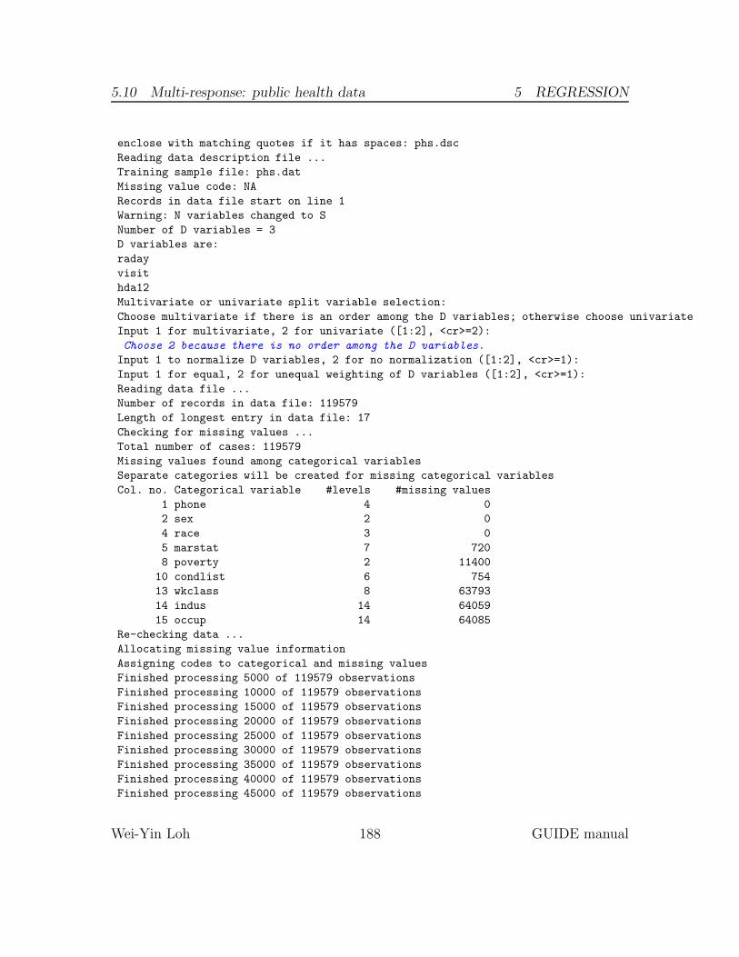
5.10 Multi-response: public health data 5 REGRESSION
enclose with matching quotes if it has spaces: phs.dsc
Reading data description file ...
Training sample file: phs.dat
Missing value code: NA
Records in data file start on line 1
Warning: N variables changed to S
Number of D variables = 3
D variables are:
raday
visit
hda12
Multivariate or univariate split variable selection:
Choose multivariate if there is an order among the D variables; otherwise choose univariate
Input 1 for multivariate, 2 for univariate ([1:2], <cr>=2):
Choose 2 because there is no order among the D variables.
Input 1 to normalize D variables, 2 for no normalization ([1:2], <cr>=1):
Input 1 for equal, 2 for unequal weighting of D variables ([1:2], <cr>=1):
Reading data file ...
Number of records in data file: 119579
Length of longest entry in data file: 17
Checking for missing values ...
Total number of cases: 119579
Missing values found among categorical variables
Separate categories will be created for missing categorical variables
Col. no. Categorical variable #levels #missing values
1 phone 4 0
2 sex 2 0
4 race 3 0
5 marstat 7 720
8 poverty 2 11400
10 condlist 6 754
13 wkclass 8 63793
14 indus 14 64059
15 occup 14 64085
Re-checking data ...
Allocating missing value information
Assigning codes to categorical and missing values
Finished processing 5000 of 119579 observations
Finished processing 10000 of 119579 observations
Finished processing 15000 of 119579 observations
Finished processing 20000 of 119579 observations
Finished processing 25000 of 119579 observations
Finished processing 30000 of 119579 observations
Finished processing 35000 of 119579 observations
Finished processing 40000 of 119579 observations
Finished processing 45000 of 119579 observations
Wei-Yin Loh 188 GUIDE manual

5.10 Multi-response: public health data 5 REGRESSION
Finished processing 50000 of 119579 observations
Finished processing 55000 of 119579 observations
Finished processing 60000 of 119579 observations
Finished processing 65000 of 119579 observations
Finished processing 70000 of 119579 observations
Finished processing 75000 of 119579 observations
Finished processing 80000 of 119579 observations
Finished processing 85000 of 119579 observations
Finished processing 90000 of 119579 observations
Finished processing 95000 of 119579 observations
Finished processing 100000 of 119579 observations
Finished processing 105000 of 119579 observations
Finished processing 110000 of 119579 observations
Finished processing 115000 of 119579 observations
Data checks complete
Normalizing data
Creating missing value indicators
Some D variables have missing values
You can use all the data or only those with complete D values
Using only cases with complete D values will reduce the sample size
but allows the option of using PCA for split selection
Input 1 to use all obs, 2 to use obs with complete D values ([1:2], <cr>=2):
Using only observations with complete D values allows more options.
Rereading data
PCA can be used for variable selection
Do not use PCA if differential item functioning (DIF) scores are wanted
Input 1 to use PCA, 2 otherwise ([1:2], <cr>=2):
#cases w/ miss. D = number of cases with all D values missing
Total #cases w/ #missing
#cases miss. D ord. vals #X-var #N-var #F-var #S-var #B-var #C-var
119579 0 30722 2 0 0 6 0 9
No. cases used for training: 60000
No. cases excluded due to 0 weight or missing D: 59579
Finished reading data file
Input 1 for LaTeX tree code, 2 to skip it ([1:2], <cr>=1):
Input file name to store LaTeX code (use .tex as suffix): mult.tex
Input 2 to save node IDs of observations, 1 otherwise ([1:2], <cr>=2):
Input name of file to store terminal node ID of each case: mult.nid
Input 2 to save fitted values at each terminal node; 1 otherwise ([1:2], <cr>=1): 2
Input name of file to store node fitted values: mult.fit
Input 2 to write R function for predicting new cases, 1 otherwise ([1:2], <cr>=1):
Input file is created!
Run GUIDE with the command: guide < mult.in
Wei-Yin Loh 189 GUIDE manual
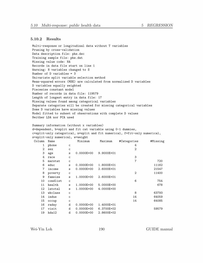
5.10 Multi-response: public health data 5 REGRESSION
5.10.2 Results
Multi-response or longitudinal data without T variables
Pruning by cross-validation
Data description file: phs.dsc
Training sample file: phs.dat
Missing value code: NA
Records in data file start on line 1
Warning: N variables changed to S
Number of D variables = 3
Univariate split variable selection method
Mean-squared errors (MSE) are calculated from normalized D variables
D variables equally weighted
Piecewise constant model
Number of records in data file: 119579
Length of longest entry in data file: 17
Missing values found among categorical variables
Separate categories will be created for missing categorical variables
Some D variables have missing values
Model fitted to subset of observations with complete D values
Neither LDA nor PCA used
Summary information (without x variables)
d=dependent, b=split and fit cat variable using 0-1 dummies,
c=split-only categorical, n=split and fit numerical, f=fit-only numerical,
s=split-only numerical, w=weight
Column Name Minimum Maximum #Categories #Missing
1 phone c 4
2 sex c 2
3 age s 0.0000E+00 9.9000E+01
4 race c 3
5 marstat c 7 720
6 educ s 0.0000E+00 1.8000E+01 11162
7 income s 0.0000E+00 2.6000E+01 21547
8 poverty c 2 11400
9 famsize s 1.0000E+00 2.6000E+01
10 condlist c 6 754
11 health s 1.0000E+00 5.0000E+00 678
12 latotal s 1.0000E+00 4.0000E+00
13 wkclass c 8 63793
14 indus c 14 64059
15 occup c 14 64085
16 raday d 0.0000E+00 1.4000E+01
17 visit d 0.0000E+00 6.3700E+02 59579
19 hda12 d 0.0000E+00 2.8600E+02
Wei-Yin Loh 190 GUIDE manual
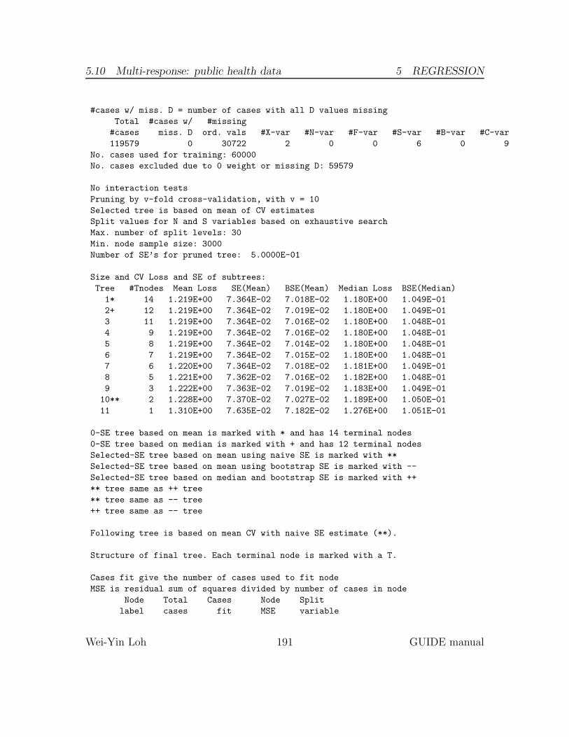
5.10 Multi-response: public health data 5 REGRESSION
#cases w/ miss. D = number of cases with all D values missing
Total #cases w/ #missing
#cases miss. D ord. vals #X-var #N-var #F-var #S-var #B-var #C-var
119579 0 30722 2 0 0 6 0 9
No. cases used for training: 60000
No. cases excluded due to 0 weight or missing D: 59579
No interaction tests
Pruning by v-fold cross-validation, with v = 10
Selected tree is based on mean of CV estimates
Split values for N and S variables based on exhaustive search
Max. number of split levels: 30
Min. node sample size: 3000
Number of SE’s for pruned tree: 5.0000E-01
Size and CV Loss and SE of subtrees:
Tree #Tnodes Mean Loss SE(Mean) BSE(Mean) Median Loss BSE(Median)
1* 14 1.219E+00 7.364E-02 7.018E-02 1.180E+00 1.049E-01
2+ 12 1.219E+00 7.364E-02 7.019E-02 1.180E+00 1.049E-01
3 11 1.219E+00 7.364E-02 7.016E-02 1.180E+00 1.048E-01
4 9 1.219E+00 7.364E-02 7.016E-02 1.180E+00 1.048E-01
5 8 1.219E+00 7.364E-02 7.014E-02 1.180E+00 1.048E-01
6 7 1.219E+00 7.364E-02 7.015E-02 1.180E+00 1.048E-01
7 6 1.220E+00 7.364E-02 7.018E-02 1.181E+00 1.049E-01
8 5 1.221E+00 7.362E-02 7.016E-02 1.182E+00 1.048E-01
9 3 1.222E+00 7.363E-02 7.019E-02 1.183E+00 1.049E-01
10** 2 1.228E+00 7.370E-02 7.027E-02 1.189E+00 1.050E-01
11 1 1.310E+00 7.635E-02 7.182E-02 1.276E+00 1.051E-01
0-SE tree based on mean is marked with * and has 14 terminal nodes
0-SE tree based on median is marked with + and has 12 terminal nodes
Selected-SE tree based on mean using naive SE is marked with **
Selected-SE tree based on mean using bootstrap SE is marked with --
Selected-SE tree based on median and bootstrap SE is marked with ++
** tree same as ++ tree
** tree same as -- tree
++ tree same as -- tree
Following tree is based on mean CV with naive SE estimate (**).
Structure of final tree. Each terminal node is marked with a T.
Cases fit give the number of cases used to fit node
MSE is residual sum of squares divided by number of cases in node
Node Total Cases Node Split
label cases fit MSE variable
Wei-Yin Loh 191 GUIDE manual
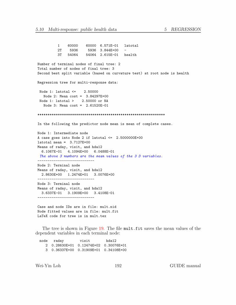
5.10 Multi-response: public health data 5 REGRESSION
1 60000 60000 6.571E-01 latotal
2T 5936 5936 3.844E+00 -
3T 54064 54064 2.615E-01 health
Number of terminal nodes of final tree: 2
Total number of nodes of final tree: 3
Second best split variable (based on curvature test) at root node is health
Regression tree for multi-response data:
Node 1: latotal <= 2.50000
Node 2: Mean cost = 3.84297E+00
Node 1: latotal > 2.50000 or NA
Node 3: Mean cost = 2.61520E-01
***************************************************************
In the following the predictor node mean is mean of complete cases.
Node 1: Intermediate node
A case goes into Node 2 if latotal <= 2.5000000E+00
latotal mean = 3.7127E+00
Means of raday, visit, and hda12
6.1067E-01 4.1094E+00 6.0488E-01
The above 3 numbers are the mean values of the 3 D variables.
----------------------------
Node 2: Terminal node
Means of raday, visit, and hda12
2.8630E+00 1.2474E+01 3.0076E+00
----------------------------
Node 3: Terminal node
Means of raday, visit, and hda12
3.6337E-01 3.1909E+00 3.4108E-01
----------------------------
Case and node IDs are in file: mult.nid
Node fitted values are in file: mult.fit
LaTeX code for tree is in mult.tex
The tree is shown in Figure 19. The file mult.fit saves the mean values of thedependent variables in each terminal node:
node raday visit hda12
2 0.28630E+01 0.12474E+02 0.30076E+01
3 0.36337E+00 0.31909E+01 0.34108E+00
Wei-Yin Loh 192 GUIDE manual

5.11 Longitudinal response with varying time: wage data 5 REGRESSION
latotal≤ 2.50 1
2
59362.86312.473.008
3
540640.3633.1910.341
Figure 19: GUIDE v.27.9 0.50-SE regression tree for predicting response variablesraday, visit, and hda12. PCA not used. Maximum number of split levels is 30 andminimum node sample size is 3000. At each split, an observation goes to the leftbranch if and only if the condition is satisfied. Sample sizes (in italics) and predictedvalues of raday, visit, and hda12 printed below nodes. Second best split variableat root node is health.
The file mult.nid gives the terminal node number for each observation, includingthose that are not used to construct the tree (indicated by the letter “n” in the traincolumn of the file).
5.11 Longitudinal response with varying time: wage data
The data come from a longitudinal study on the hourly wage of 888 male high-school dropouts (246 black, 204 Hispanic, 438 white), where the observation timepoints as well as their number (1–13) varied across individuals (Murnane et al., 1999;Singer and Willett, 2003). An earlier version of GUIDE was used to analyze the datain Loh and Zheng (2013).
The response variable is hourly wage (in 1990 dollars) and the predictor variablesare hgc (highest grade completed; 6–12), exper (years in labor force; 0.001–12.7yrs), and race (Black, Hispanic, and White). The data file wagedat.txt is in wideformat, where each record refers to one individual. The description file wagedsc.txtis given below. Note that observation time points are marked as t.
wagedat.txt
NA
1
1 id x
2 hgc n
3 exper1 t
4 exper2 t
Wei-Yin Loh 193 GUIDE manual

5.11 Longitudinal response with varying time: wage data 5 REGRESSION
5 exper3 t
6 exper4 t
7 exper5 t
8 exper6 t
9 exper7 t
10 exper8 t
11 exper9 t
12 exper10 t
13 exper11 t
14 exper12 t
15 exper13 t
16 postexp1 x
17 postexp2 x
18 postexp3 x
19 postexp4 x
20 postexp5 x
21 postexp6 x
22 postexp7 x
23 postexp8 x
24 postexp9 x
25 postexp10 x
26 postexp11 x
27 postexp12 x
28 postexp13 x
29 wage1 d
30 wage2 d
31 wage3 d
32 wage4 d
33 wage5 d
34 wage6 d
35 wage7 d
36 wage8 d
37 wage9 d
38 wage10 d
39 wage11 d
40 wage12 d
41 wage13 d
42 ged1 x
43 ged2 x
44 ged3 x
45 ged4 x
46 ged5 x
47 ged6 x
48 ged7 x
49 ged8 x
50 ged9 x
Wei-Yin Loh 194 GUIDE manual

5.11 Longitudinal response with varying time: wage data 5 REGRESSION
51 ged10 x
52 ged11 x
53 ged12 x
54 ged13 x
55 uerate1 x
56 uerate2 x
57 uerate3 x
58 uerate4 x
59 uerate5 x
60 uerate6 x
61 uerate7 x
62 uerate8 x
63 uerate9 x
64 uerate10 x
65 uerate11 x
66 uerate12 x
67 uerate13 x
68 race c
5.11.1 Input file creation
Because the default 0.5-SE rule yields a trivial tree with no splits, we show how theoptions can be changed to produce a tree with the 0-SE rule. Following is a sessionlog.
0. Read the warranty disclaimer
1. Create a GUIDE input file
Input your choice: 1
Name of batch input file: wage.in
Input 1 for model fitting, 2 for importance or DIF scoring,
3 for data conversion ([1:3], <cr>=1):
Name of batch output file: wage.out
Input 1 for single tree, 2 for ensemble ([1:2], <cr>=1):
Input 1 for classification, 2 for regression, 3 for propensity score grouping
(propensity score grouping is an experimental option)
Input your choice ([1:3], <cr>=1): 2
Choose type of regression model:
1=linear, 2=quantile, 3=Poisson, 4=proportional hazards,
5=multiresponse or itemresponse, 6=longitudinal data (with T variables).
Input choice ([1:6], <cr>=1): 6
Input 1 for lowess smoothing, 2 for spline smoothing ([1:2], <cr>=1):
Input 1 for default options, 2 otherwise ([1:2], <cr>=1): 2
Choosing 1 will produce a 0.5-SE tree. We choose 2 to allow more options.
Input 1 for interaction tests, 2 to skip them ([1:2], <cr>=1):
Input 1 to prune by CV, 2 for no pruning ([1:2], <cr>=1):
Wei-Yin Loh 195 GUIDE manual
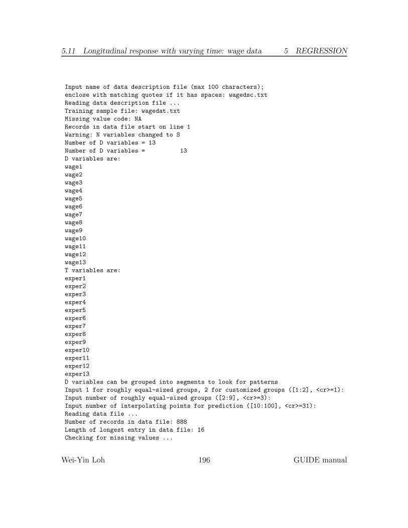
5.11 Longitudinal response with varying time: wage data 5 REGRESSION
Input name of data description file (max 100 characters);
enclose with matching quotes if it has spaces: wagedsc.txt
Reading data description file ...
Training sample file: wagedat.txt
Missing value code: NA
Records in data file start on line 1
Warning: N variables changed to S
Number of D variables = 13
Number of D variables = 13
D variables are:
wage1
wage2
wage3
wage4
wage5
wage6
wage7
wage8
wage9
wage10
wage11
wage12
wage13
T variables are:
exper1
exper2
exper3
exper4
exper5
exper6
exper7
exper8
exper9
exper10
exper11
exper12
exper13
D variables can be grouped into segments to look for patterns
Input 1 for roughly equal-sized groups, 2 for customized groups ([1:2], <cr>=1):
Input number of roughly equal-sized groups ([2:9], <cr>=3):
Input number of interpolating points for prediction ([10:100], <cr>=31):
Reading data file ...
Number of records in data file: 888
Length of longest entry in data file: 16
Checking for missing values ...
Wei-Yin Loh 196 GUIDE manual
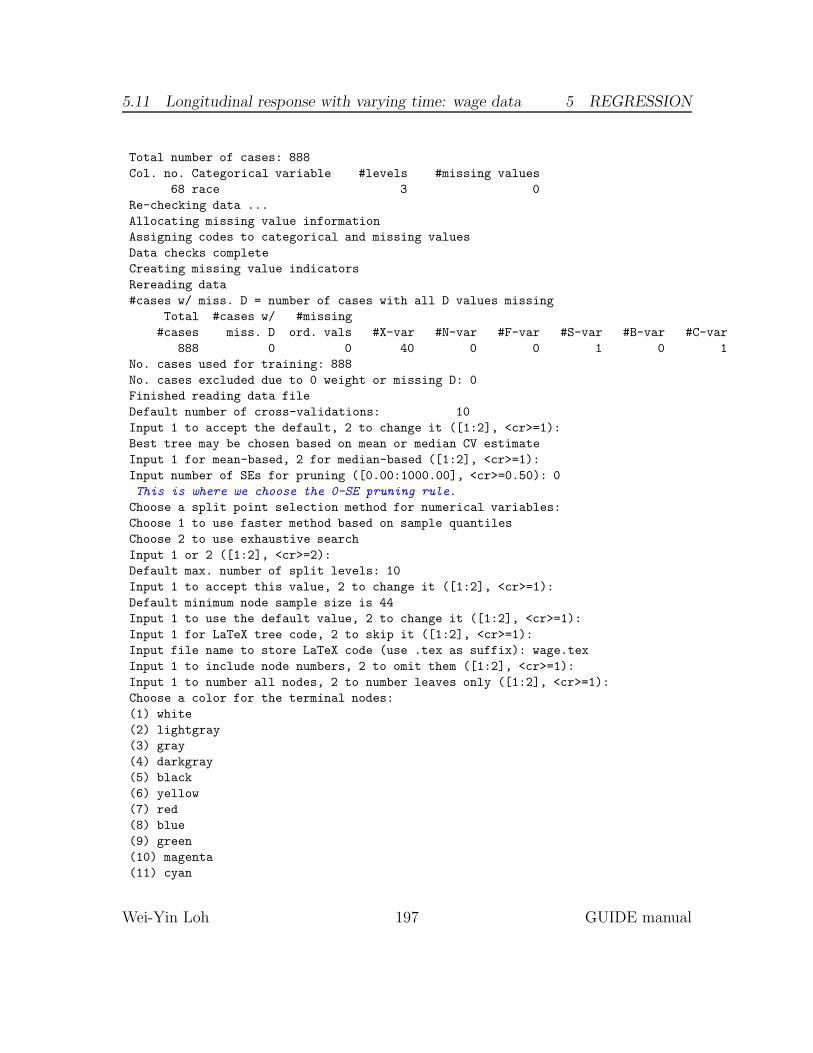
5.11 Longitudinal response with varying time: wage data 5 REGRESSION
Total number of cases: 888
Col. no. Categorical variable #levels #missing values
68 race 3 0
Re-checking data ...
Allocating missing value information
Assigning codes to categorical and missing values
Data checks complete
Creating missing value indicators
Rereading data
#cases w/ miss. D = number of cases with all D values missing
Total #cases w/ #missing
#cases miss. D ord. vals #X-var #N-var #F-var #S-var #B-var #C-var
888 0 0 40 0 0 1 0 1
No. cases used for training: 888
No. cases excluded due to 0 weight or missing D: 0
Finished reading data file
Default number of cross-validations: 10
Input 1 to accept the default, 2 to change it ([1:2], <cr>=1):
Best tree may be chosen based on mean or median CV estimate
Input 1 for mean-based, 2 for median-based ([1:2], <cr>=1):
Input number of SEs for pruning ([0.00:1000.00], <cr>=0.50): 0
This is where we choose the 0-SE pruning rule.
Choose a split point selection method for numerical variables:
Choose 1 to use faster method based on sample quantiles
Choose 2 to use exhaustive search
Input 1 or 2 ([1:2], <cr>=2):
Default max. number of split levels: 10
Input 1 to accept this value, 2 to change it ([1:2], <cr>=1):
Default minimum node sample size is 44
Input 1 to use the default value, 2 to change it ([1:2], <cr>=1):
Input 1 for LaTeX tree code, 2 to skip it ([1:2], <cr>=1):
Input file name to store LaTeX code (use .tex as suffix): wage.tex
Input 1 to include node numbers, 2 to omit them ([1:2], <cr>=1):
Input 1 to number all nodes, 2 to number leaves only ([1:2], <cr>=1):
Choose a color for the terminal nodes:
(1) white
(2) lightgray
(3) gray
(4) darkgray
(5) black
(6) yellow
(7) red
(8) blue
(9) green
(10) magenta
(11) cyan
Wei-Yin Loh 197 GUIDE manual
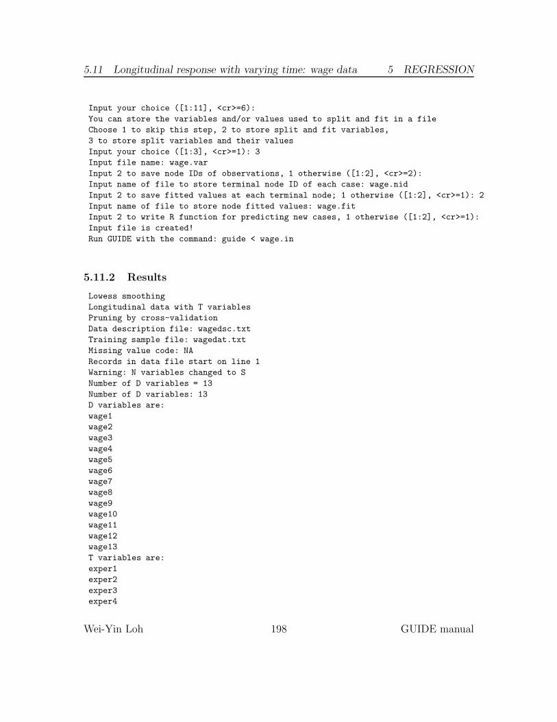
5.11 Longitudinal response with varying time: wage data 5 REGRESSION
Input your choice ([1:11], <cr>=6):
You can store the variables and/or values used to split and fit in a file
Choose 1 to skip this step, 2 to store split and fit variables,
3 to store split variables and their values
Input your choice ([1:3], <cr>=1): 3
Input file name: wage.var
Input 2 to save node IDs of observations, 1 otherwise ([1:2], <cr>=2):
Input name of file to store terminal node ID of each case: wage.nid
Input 2 to save fitted values at each terminal node; 1 otherwise ([1:2], <cr>=1): 2
Input name of file to store node fitted values: wage.fit
Input 2 to write R function for predicting new cases, 1 otherwise ([1:2], <cr>=1):
Input file is created!
Run GUIDE with the command: guide < wage.in
5.11.2 Results
Lowess smoothing
Longitudinal data with T variables
Pruning by cross-validation
Data description file: wagedsc.txt
Training sample file: wagedat.txt
Missing value code: NA
Records in data file start on line 1
Warning: N variables changed to S
Number of D variables = 13
Number of D variables: 13
D variables are:
wage1
wage2
wage3
wage4
wage5
wage6
wage7
wage8
wage9
wage10
wage11
wage12
wage13
T variables are:
exper1
exper2
exper3
exper4
Wei-Yin Loh 198 GUIDE manual
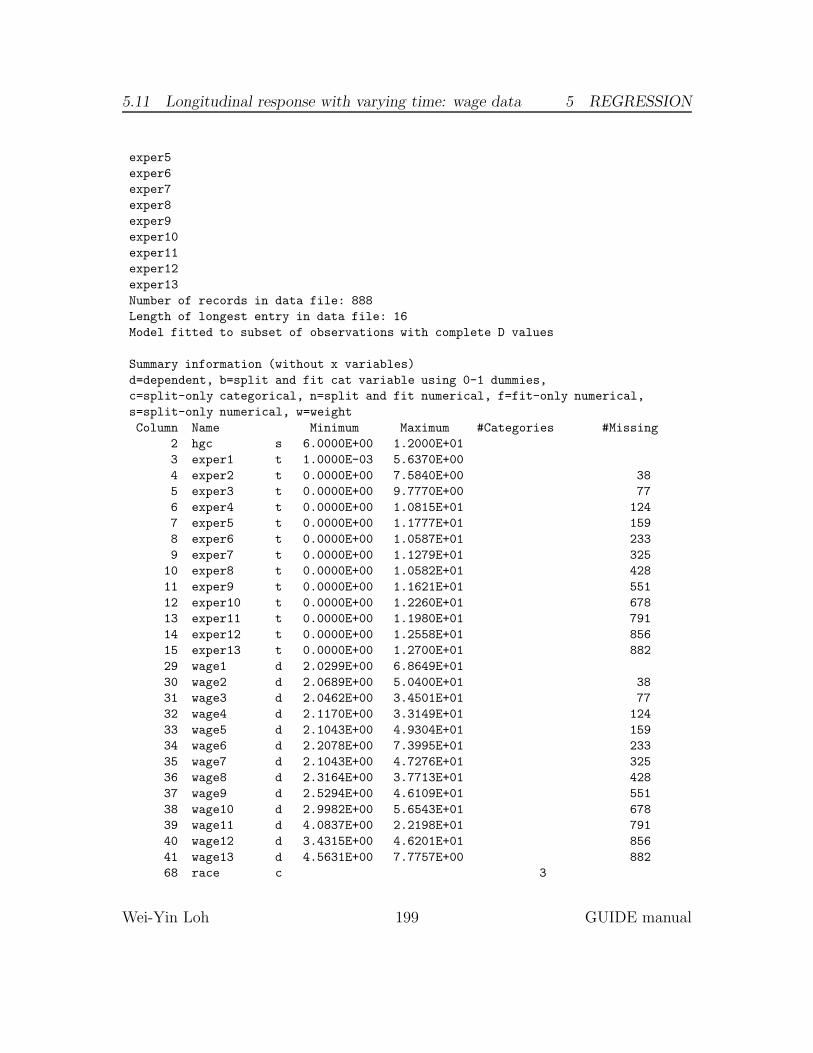
5.11 Longitudinal response with varying time: wage data 5 REGRESSION
exper5
exper6
exper7
exper8
exper9
exper10
exper11
exper12
exper13
Number of records in data file: 888
Length of longest entry in data file: 16
Model fitted to subset of observations with complete D values
Summary information (without x variables)
d=dependent, b=split and fit cat variable using 0-1 dummies,
c=split-only categorical, n=split and fit numerical, f=fit-only numerical,
s=split-only numerical, w=weight
Column Name Minimum Maximum #Categories #Missing
2 hgc s 6.0000E+00 1.2000E+01
3 exper1 t 1.0000E-03 5.6370E+00
4 exper2 t 0.0000E+00 7.5840E+00 38
5 exper3 t 0.0000E+00 9.7770E+00 77
6 exper4 t 0.0000E+00 1.0815E+01 124
7 exper5 t 0.0000E+00 1.1777E+01 159
8 exper6 t 0.0000E+00 1.0587E+01 233
9 exper7 t 0.0000E+00 1.1279E+01 325
10 exper8 t 0.0000E+00 1.0582E+01 428
11 exper9 t 0.0000E+00 1.1621E+01 551
12 exper10 t 0.0000E+00 1.2260E+01 678
13 exper11 t 0.0000E+00 1.1980E+01 791
14 exper12 t 0.0000E+00 1.2558E+01 856
15 exper13 t 0.0000E+00 1.2700E+01 882
29 wage1 d 2.0299E+00 6.8649E+01
30 wage2 d 2.0689E+00 5.0400E+01 38
31 wage3 d 2.0462E+00 3.4501E+01 77
32 wage4 d 2.1170E+00 3.3149E+01 124
33 wage5 d 2.1043E+00 4.9304E+01 159
34 wage6 d 2.2078E+00 7.3995E+01 233
35 wage7 d 2.1043E+00 4.7276E+01 325
36 wage8 d 2.3164E+00 3.7713E+01 428
37 wage9 d 2.5294E+00 4.6109E+01 551
38 wage10 d 2.9982E+00 5.6543E+01 678
39 wage11 d 4.0837E+00 2.2198E+01 791
40 wage12 d 3.4315E+00 4.6201E+01 856
41 wage13 d 4.5631E+00 7.7757E+00 882
68 race c 3
Wei-Yin Loh 199 GUIDE manual
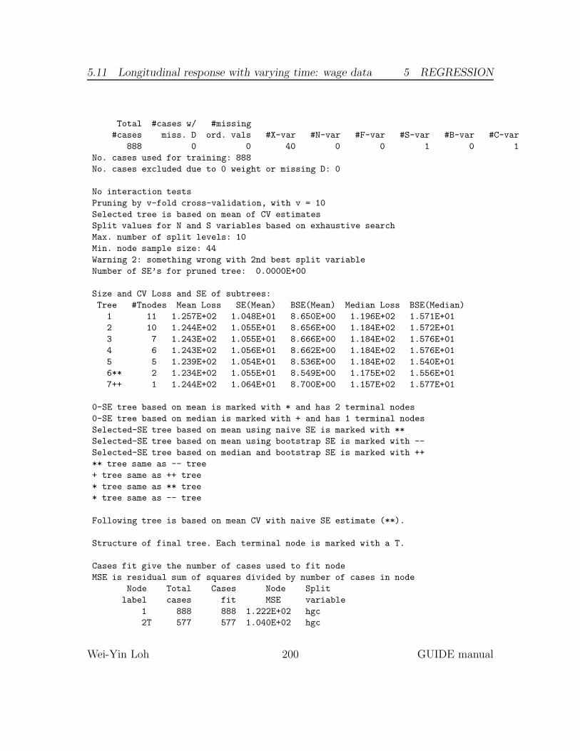
5.11 Longitudinal response with varying time: wage data 5 REGRESSION
Total #cases w/ #missing
#cases miss. D ord. vals #X-var #N-var #F-var #S-var #B-var #C-var
888 0 0 40 0 0 1 0 1
No. cases used for training: 888
No. cases excluded due to 0 weight or missing D: 0
No interaction tests
Pruning by v-fold cross-validation, with v = 10
Selected tree is based on mean of CV estimates
Split values for N and S variables based on exhaustive search
Max. number of split levels: 10
Min. node sample size: 44
Warning 2: something wrong with 2nd best split variable
Number of SE’s for pruned tree: 0.0000E+00
Size and CV Loss and SE of subtrees:
Tree #Tnodes Mean Loss SE(Mean) BSE(Mean) Median Loss BSE(Median)
1 11 1.257E+02 1.048E+01 8.650E+00 1.196E+02 1.571E+01
2 10 1.244E+02 1.055E+01 8.656E+00 1.184E+02 1.572E+01
3 7 1.243E+02 1.055E+01 8.666E+00 1.184E+02 1.576E+01
4 6 1.243E+02 1.056E+01 8.662E+00 1.184E+02 1.576E+01
5 5 1.239E+02 1.054E+01 8.536E+00 1.184E+02 1.540E+01
6** 2 1.234E+02 1.055E+01 8.549E+00 1.175E+02 1.556E+01
7++ 1 1.244E+02 1.064E+01 8.700E+00 1.157E+02 1.577E+01
0-SE tree based on mean is marked with * and has 2 terminal nodes
0-SE tree based on median is marked with + and has 1 terminal nodes
Selected-SE tree based on mean using naive SE is marked with **
Selected-SE tree based on mean using bootstrap SE is marked with --
Selected-SE tree based on median and bootstrap SE is marked with ++
** tree same as -- tree
+ tree same as ++ tree
* tree same as ** tree
* tree same as -- tree
Following tree is based on mean CV with naive SE estimate (**).
Structure of final tree. Each terminal node is marked with a T.
Cases fit give the number of cases used to fit node
MSE is residual sum of squares divided by number of cases in node
Node Total Cases Node Split
label cases fit MSE variable
1 888 888 1.222E+02 hgc
2T 577 577 1.040E+02 hgc
Wei-Yin Loh 200 GUIDE manual
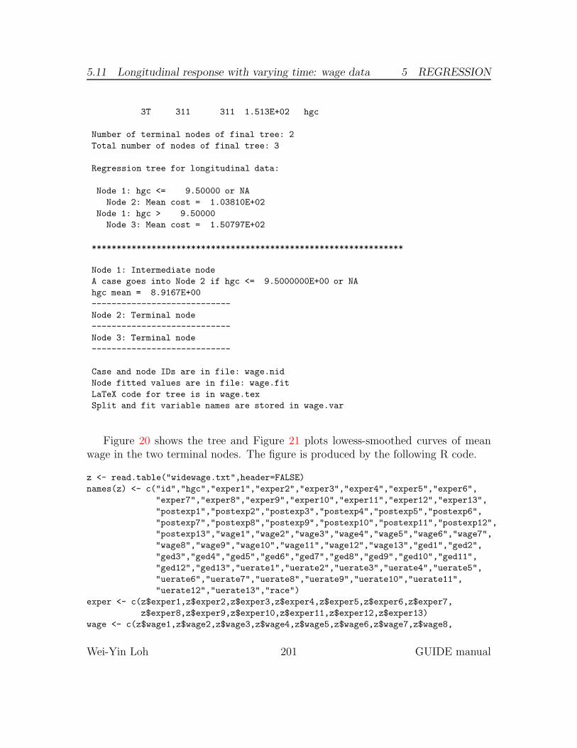
5.11 Longitudinal response with varying time: wage data 5 REGRESSION
3T 311 311 1.513E+02 hgc
Number of terminal nodes of final tree: 2
Total number of nodes of final tree: 3
Regression tree for longitudinal data:
Node 1: hgc <= 9.50000 or NA
Node 2: Mean cost = 1.03810E+02
Node 1: hgc > 9.50000
Node 3: Mean cost = 1.50797E+02
***************************************************************
Node 1: Intermediate node
A case goes into Node 2 if hgc <= 9.5000000E+00 or NA
hgc mean = 8.9167E+00
----------------------------
Node 2: Terminal node
----------------------------
Node 3: Terminal node
----------------------------
Case and node IDs are in file: wage.nid
Node fitted values are in file: wage.fit
LaTeX code for tree is in wage.tex
Split and fit variable names are stored in wage.var
Figure 20 shows the tree and Figure 21 plots lowess-smoothed curves of meanwage in the two terminal nodes. The figure is produced by the following R code.
z <- read.table("widewage.txt",header=FALSE)
names(z) <- c("id","hgc","exper1","exper2","exper3","exper4","exper5","exper6",
"exper7","exper8","exper9","exper10","exper11","exper12","exper13",
"postexp1","postexp2","postexp3","postexp4","postexp5","postexp6",
"postexp7","postexp8","postexp9","postexp10","postexp11","postexp12",
"postexp13","wage1","wage2","wage3","wage4","wage5","wage6","wage7",
"wage8","wage9","wage10","wage11","wage12","wage13","ged1","ged2",
"ged3","ged4","ged5","ged6","ged7","ged8","ged9","ged10","ged11",
"ged12","ged13","uerate1","uerate2","uerate3","uerate4","uerate5",
"uerate6","uerate7","uerate8","uerate9","uerate10","uerate11",
"uerate12","uerate13","race")
exper <- c(z$exper1,z$exper2,z$exper3,z$exper4,z$exper5,z$exper6,z$exper7,
z$exper8,z$exper9,z$exper10,z$exper11,z$exper12,z$exper13)
wage <- c(z$wage1,z$wage2,z$wage3,z$wage4,z$wage5,z$wage6,z$wage7,z$wage8,
Wei-Yin Loh 201 GUIDE manual

5.11 Longitudinal response with varying time: wage data 5 REGRESSION
z$wage9,z$wage10,z$wage11,z$wage12,z$wage13)
xr <- range(exper,na.rm=TRUE)
yr <- range(wage,na.rm=TRUE)
guide.fit <- read.table("wage.fit",header=TRUE)
g.node <- guide.fit$node
g.start <- guide.fit$t.start
g.end <- guide.fit$t.end
n <- length(g.node)
m <- dim(guide.fit)[2]
npts <- m-3 # number of time points for plotting
xvals <- guide.fit[,2:3]
xvals <- as.numeric(unlist(xvals))
yvals <- guide.fit[,4:m]
yvals <- as.numeric(unlist(yvals))
plot(range(xvals),range(yvals),type="n",xlab="exper (years)",ylab="hourly wage ($)")
leg.col <- c("red","black")
leg.lty <- c(1,2)
for(i in 1:n){
node <- g.node[i]
start <- g.start[i]
end <- g.end[i]
gap <- (end-start)/(npts-1)
x <- start+(0:(npts-1))*gap
y <- as.numeric(guide.fit[i,4:m])
lines(x,y,col=leg.col[i],lty=leg.lty[i])
}
leg.txt <- c(expression(paste("hgc" <= 9)),
expression(paste("hgc" > 9)))
legend("topleft",legend=leg.txt,lty=leg.lty,col=leg.col,lwd=2)
The plotting values are obtained from the result file wage.fit whose contents aregiven below. The first column gives the node number and the next two columns thestart and end of the times at which fitted values are computed. The other columnsgive the fitted values equally spaced between the start and end times.
node t.start t.end fitted1 fitted2 fitted3 fitted4 fitted5 fitted6 fitted7 fitted8 fitted9 fitted10
2 0.10000E-02 0.12700E+02 0.48875E+01 0.51221E+01 0.53241E+01 0.54668E+01 0.55738E+01 0.56948E+01
3 0.20000E-02 0.12558E+02 0.57699E+01 0.58884E+01 0.60035E+01 0.60997E+01 0.61994E+01 0.63206E+01
The contents of the file wage.var are given below. The 1st column gives thenode number. Te 2nd column is a letter, with t indicating that the node is terminal
Wei-Yin Loh 202 GUIDE manual
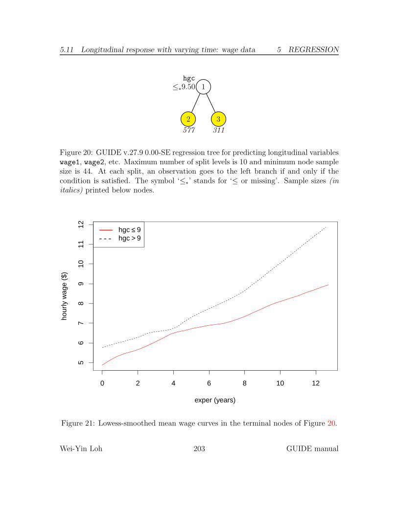
5.11 Longitudinal response with varying time: wage data 5 REGRESSION
hgc≤∗9.50 1
2
577
3
311
Figure 20: GUIDE v.27.9 0.00-SE regression tree for predicting longitudinal variableswage1, wage2, etc. Maximum number of split levels is 10 and minimum node samplesize is 44. At each split, an observation goes to the left branch if and only if thecondition is satisfied. The symbol ‘≤∗’ stands for ‘≤ or missing’. Sample sizes (initalics) printed below nodes.
0 2 4 6 8 10 12
56
78
910
1112
exper (years)
hour
ly w
age
($)
hgc ≤ 9hgc > 9
Figure 21: Lowess-smoothed mean wage curves in the terminal nodes of Figure 20.
Wei-Yin Loh 203 GUIDE manual

5.12 Subgroup identification: breast cancer 5 REGRESSION
and c, s, or n indicating an intermediate node split on a c, n or s variable. The 3rdcolumn gives the name of the variable used to split the node; the name NONE is usedif a terminal node cannot be split by any variable. The 4th column gives the nameof the interacting variable if there is one; otherwise the name of the split variable isrepeated. For a non-terminal node, the integer in the 5th column gives the numberof split values to follow on the line.
1 s hgc hgc 1 0.9500000000E+01
2 t hgc hgc 0.0000000000E+00
3 t hgc hgc 0.0000000000E+00
5.12 Subgroup identification: breast cancer
GUIDE has several methods to identify subgroups for differential treatment effectsfrom randomized experiments. See Loh et al. (2015) and Loh et al. (2016) for details.The treatment variable is assumed to be categorical (i.e., it takes nominal values)and the response is an uncensored or censored event time (e.g., survival time). Thekey points are:
1. The treatment variable is designated as R (for “Rx”).
2. If there is no censoring in the response, it is designated as the dependentvariable as D as usual.
3. If there is censoring in the response, the variable is designated as T (first letterof “Time”). In this case, the event indicator is designated as D (first letter of“Death”) and takes value 1 if the event (“death”) occurs and 0 if the eventtime is censored.
There are two types of covariate variables in subgroup identification. A prognos-tic variable is a clinical or biologic characteristic that provides information on thelikely outcome of the disease in an untreated individual (e.g., patient age, familyhistory, disease stage, and prior therapy). A predictive variable is a characteristicthat provides information on the likely benefit from treatment. Predictive variablescan be used to identify subgroups of patients who are most likely to benefit from agiven therapy. Therefore prognostic variables define the effects of patient or tumorcharacteristics on the patient outcome, whereas predictive variables define the effectof treatment on the tumor (Italiano, 2011). Accordingly, GUIDE has two methods,called Gi and Gs. Gi is more sensitive to predictive variables and Gs tends to beequally sensitive to prognostic and predictive variables (Loh et al., 2015).
Wei-Yin Loh 204 GUIDE manual

5.12 Subgroup identification: breast cancer 5 REGRESSION
5.12.1 Without linear prognostic control
The simplest model only uses the covariates to split the intermediate nodes; termi-nal nodes are fitted with treatment means. We use a data set from a randomizedcontrolled breast cancer trial (Schmoor et al., 1996) to show this. The data are inthe file cancer.txt; it can also be obtained from the TH.data R package (Hothorn,2017). In the description file cancerdsc.txt below, the treatment variable is hor-mone therapy, horTh. The variable time is (censored) time to recurrence of cancerand event = 1 if the cancer recurred and = 0 if it did not. Ordinal predictor variablesmay be designated as “n” or “s” (with this option of no linear prognostic control, nvariables will be automatically changed to s when the program is executed).
cancer.txt
NA
1
1 horTh r
2 age n
3 menostat c
4 tsize n
5 tgrade c
6 pnodes n
7 progrec n
8 estrec n
9 time t
10 event d
Input file generation
0. Read the warranty disclaimer
1. Create a GUIDE input file
Input your choice: 1
Name of batch input file: nolin.in
Input 1 for model fitting, 2 for importance or DIF scoring,
3 for data conversion ([1:3], <cr>=1):
Name of batch output file: nolin.out
Input 1 for single tree, 2 for ensemble ([1:2], <cr>=1):
Input 1 for classification, 2 for regression, 3 for propensity score grouping
(propensity score grouping is an experimental option)
Input your choice ([1:3], <cr>=1): 2
Choose type of regression model:
1=linear, 2=quantile, 3=Poisson, 4=proportional hazards,
5=multiresponse or itemresponse, 6=longitudinal data (with T variables).
Input choice ([1:6], <cr>=1): 4
Choose complexity of model to use at each node:
Choose 1 for multiple regression (recommended if R variable is present,
unless there are too many N, F or B variables)
Wei-Yin Loh 205 GUIDE manual

5.12 Subgroup identification: breast cancer 5 REGRESSION
Choose 2 for best polynomial in one N or F variable + R (if present)
Choose 3 to fit a constant + R (if present)
1: multiple linear, 2: best polynomial, 3: constant ([1:3], <cr>=3):
Option 3 is the one for no linear prognostic control.
Input 1 for default options, 2 otherwise ([1:2], <cr>=1): 2
Input 1 for interaction tests, 2 to skip them ([1:2], <cr>=1):
Input 1 to prune by CV, 2 for no pruning ([1:2], <cr>=1):
Input name of data description file (max 100 characters);
enclose with matching quotes if it has spaces: cancerdsc.txt
Reading data description file ...
Training sample file: cancer.txt
Missing value code: NA
Records in data file start on line 1
R variable present
Warning: N variables changed to S
Warning: model changed to linear in treatment
Warnings due to presence of R variable and choice of no linear prognostic effects.
Dependent variable is death
Reading data file ...
Number of records in data file: 686
Length of longest entry in data file: 4
Checking for missing values ...
Total number of cases: 686
Col. no. Categorical variable #levels #missing values
1 horTh 2 0
3 menostat 2 0
Treatment (R) variable is horTh with values "no" and "yes"
Re-checking data ...
Assigning codes to categorical and missing values
Data checks complete
Smallest uncensored T: 72.00
No. cases dropped due to missing D or T or censored T < smallest uncensored T: 14
No. complete cases excluding censored T < smallest uncensored T: 672
No. cases used to compute baseline hazard: 672
No. cases with D=1 and T >= smallest uncensored: 299
GUIDE will try to create the variables in the description file.
If it is unsuccessful, please create the columns yourself...
Number of dummy variables created: 1
Choose a subgroup identification method:
1 = Sum of chi-squares (Gs)
2 = Treatment interactions (Gi)
Input your choice: ([1:2], <cr>=2):
Gi is the choice if splitting on predictive variables is preferred.
Creating dummy variables
Rereading data
Wei-Yin Loh 206 GUIDE manual

5.12 Subgroup identification: breast cancer 5 REGRESSION
Total #cases w/ #missing
#cases miss. D ord. vals #X-var #N-var #F-var #S-var #B-var #C-var #R-var
686 0 0 0 0 0 6 0 1 1
Survival time variable in column: 9
Event indicator variable in column: 10
Proportion uncensored among nonmissing T and D variables: .445
No. cases used for training: 672
Finished reading data file
Choose how you wish to deal with missing values in training or test data:
Option 1: Fit separate models to complete and incomplete cases
Option 2: Impute missing F and N values at each node with means for regression
Option 3: Fit a piecewise constant model
Input selection: ([1:3], <cr>=2):
Default number of cross-validations: 10
Input 1 to accept the default, 2 to change it ([1:2], <cr>=1):
Best tree may be chosen based on mean or median CV estimate
Input 1 for mean-based, 2 for median-based ([1:2], <cr>=1):
Input number of SEs for pruning ([0.00:1000.00], <cr>=0.50):
Choose fraction of cases for splitting
Larger values give more splits: 0 = median split and 1 = all possible splits
Default fraction is 1.0000
Choose 1 to accept default split fraction, 2 to change it
Input 1 or 2 ([1:2], <cr>=1):
Default max. number of split levels: 10
Input 1 to accept this value, 2 to change it ([1:2], <cr>=1):
Default min. cases per treatment in each node is 2
Input 1 to use the default value, 2 to change it ([1:2], <cr>=1):
Default minimum node sample size is 33
Input 1 to use the default value, 2 to change it ([1:2], <cr>=1):
Input number of iterations ([1:100], <cr>=5):
Input 1 for LaTeX tree code, 2 to skip it ([1:2], <cr>=1):
Input file name to store LaTeX code (use .tex as suffix): nolin.tex
A file by that name exists
Input 1 to overwrite it, 2 to choose another name ([1:2], <cr>=1):
Input 1 to include node numbers, 2 to omit them ([1:2], <cr>=1):
Input 1 to number all nodes, 2 to number leaves only ([1:2], <cr>=1):
Choose a color for the terminal nodes:
(1) white
(2) lightgray
(3) gray
(4) darkgray
(5) black
(6) yellow
(7) red
(8) blue
(9) green
Wei-Yin Loh 207 GUIDE manual

5.12 Subgroup identification: breast cancer 5 REGRESSION
(10) magenta
(11) cyan
Input your choice ([1:11], <cr>=6):
Input 1 to print treatment effects in tree, 2 otherwise ([1:2], <cr>=1):
You can store the variables and/or values used to split and fit in a file
Choose 1 to skip this step, 2 to store split and fit variables,
3 to store split variables and their values
Input your choice ([1:3], <cr>=1):
Input 2 to save truncation limits and regression coefficients in a file, 1 otherwise ([1:2], <cr>=1):
Input 2 to save fitted values and node IDs, 1 otherwise ([1:2], <cr>=2):
Input name of file to store node ID and fitted value of each case: nolin.fit
A file by that name exists
Input 1 to overwrite it, 2 to choose another name ([1:2], <cr>=1):
Input 2 to write R function for predicting new cases, 1 otherwise ([1:2], <cr>=1):
Input file is created!
Run GUIDE with the command: guide < nolin.in
Results The contents of nolin.out follow.
Proportional hazards regression with relative risk estimates
Pruning by cross-validation
Data description file: cancerdsc.txt
Training sample file: cancer.txt
Missing value code: NA
Records in data file start on line 1
R variable present
Warning: N variables changed to S
Warning: model changed to linear in treatment
Dependent variable is death
Piecewise linear model
Number of records in data file: 686
Length of longest entry in data file: 4
Treatment (R) variable is horTh with values "no" and "yes"
Smallest uncensored T: 72.00
No. cases dropped due to missing D or T or censored T < smallest uncensored T: 14
No. complete cases excluding censored T < smallest uncensored T: 672
No. cases used to compute baseline hazard: 672
No. cases with D=1 and T >= smallest uncensored: 299
Number of dummy variables created: 1
Summary information (without x variables)
d=dependent, b=split and fit cat variable using 0-1 dummies,
c=split-only categorical, n=split and fit numerical, f=fit-only numerical,
s=split-only numerical, w=weight
t=survival time variable
Wei-Yin Loh 208 GUIDE manual

5.12 Subgroup identification: breast cancer 5 REGRESSION
Column Name Minimum Maximum #Categories #Missing
1 horTh r 2
2 age s 2.1000E+01 8.0000E+01
3 menostat c 2
4 tsize s 3.0000E+00 1.2000E+02
5 tgrade s 1.0000E+00 3.0000E+00
6 pnodes s 1.0000E+00 5.1000E+01
7 progrec s 0.0000E+00 2.3800E+03
8 estrec s 0.0000E+00 1.1440E+03
9 time t 7.2000E+01 2.6590E+03
10 death d 0.0000E+00 1.0000E+00
=================== Constructed variables ===================
11 lnbasehaz0 z -6.5103E+00 5.8866E-02
12 horTh.yes f 0.0000E+00 1.0000E+00
Total #cases w/ #missing
#cases miss. D ord. vals #X-var #N-var #F-var #S-var #B-var #C-var
686 0 0 0 0 0 6 0 1
Survival time variable in column: 9
Event indicator variable in column: 10
Proportion uncensored among nonmissing T and D variables: 0.445
No. cases used for training: 672
Missing values imputed with node means for regression
Treatment interactions (Gi)
No nodewise interaction tests
Pruning by v-fold cross-validation, with v = 10
Selected tree is based on mean of CV estimates
Fraction of cases used for splitting each node: 1.0000
Max. number of split levels: 10
Min. number of cases per treatment at each node: 2
Min. node sample size: 33
Number of iterations: 5
Number of SE’s for pruned tree: 5.0000E-01
Size and CV Loss and SE of subtrees:
Tree #Tnodes Mean Loss SE(Mean) BSE(Mean) Median Loss BSE(Median)
1 14 1.436E+00 5.830E-02 5.813E-02 1.408E+00 6.059E-02
2 13 1.435E+00 5.828E-02 5.837E-02 1.404E+00 5.987E-02
3 12 1.436E+00 5.821E-02 5.816E-02 1.404E+00 5.798E-02
4 11 1.433E+00 5.821E-02 5.885E-02 1.404E+00 5.918E-02
5 9 1.427E+00 5.794E-02 5.936E-02 1.391E+00 6.105E-02
6 8 1.426E+00 5.755E-02 5.927E-02 1.391E+00 6.089E-02
7 7 1.421E+00 5.705E-02 5.208E-02 1.391E+00 5.673E-02
8++ 4 1.406E+00 5.455E-02 4.406E-02 1.390E+00 3.077E-02
9** 2 1.423E+00 5.147E-02 3.705E-02 1.428E+00 4.535E-02
Wei-Yin Loh 209 GUIDE manual
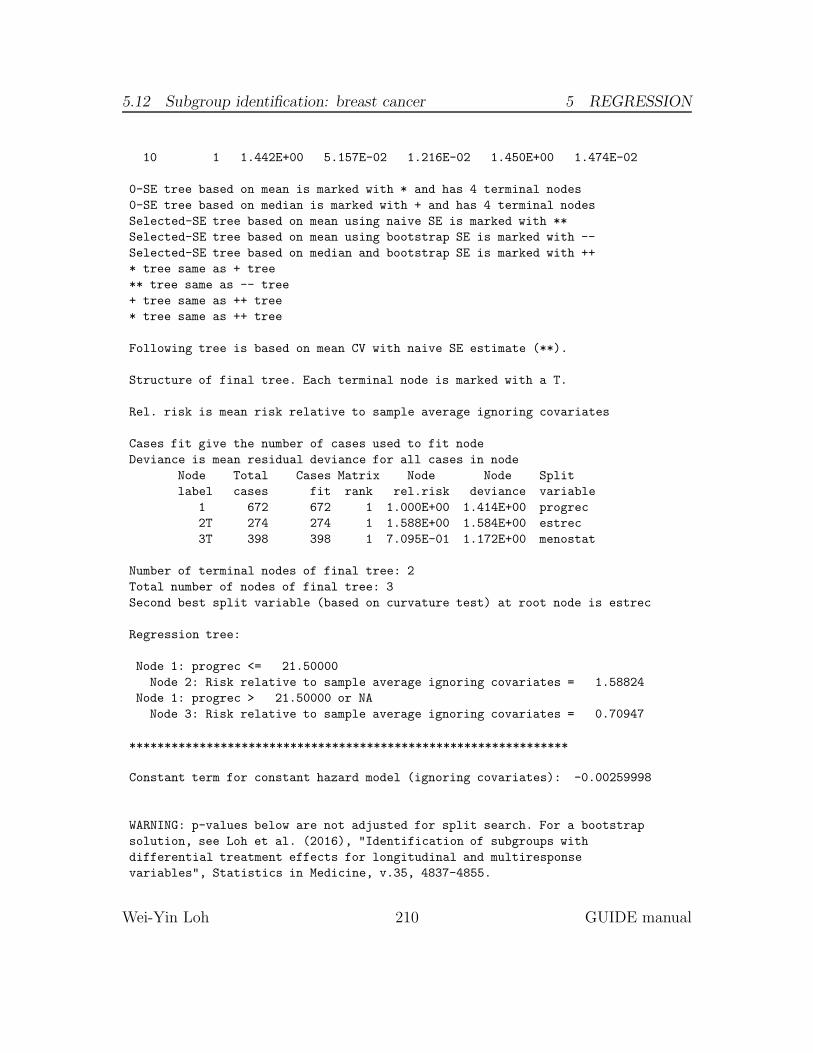
5.12 Subgroup identification: breast cancer 5 REGRESSION
10 1 1.442E+00 5.157E-02 1.216E-02 1.450E+00 1.474E-02
0-SE tree based on mean is marked with * and has 4 terminal nodes
0-SE tree based on median is marked with + and has 4 terminal nodes
Selected-SE tree based on mean using naive SE is marked with **
Selected-SE tree based on mean using bootstrap SE is marked with --
Selected-SE tree based on median and bootstrap SE is marked with ++
* tree same as + tree
** tree same as -- tree
+ tree same as ++ tree
* tree same as ++ tree
Following tree is based on mean CV with naive SE estimate (**).
Structure of final tree. Each terminal node is marked with a T.
Rel. risk is mean risk relative to sample average ignoring covariates
Cases fit give the number of cases used to fit node
Deviance is mean residual deviance for all cases in node
Node Total Cases Matrix Node Node Split
label cases fit rank rel.risk deviance variable
1 672 672 1 1.000E+00 1.414E+00 progrec
2T 274 274 1 1.588E+00 1.584E+00 estrec
3T 398 398 1 7.095E-01 1.172E+00 menostat
Number of terminal nodes of final tree: 2
Total number of nodes of final tree: 3
Second best split variable (based on curvature test) at root node is estrec
Regression tree:
Node 1: progrec <= 21.50000
Node 2: Risk relative to sample average ignoring covariates = 1.58824
Node 1: progrec > 21.50000 or NA
Node 3: Risk relative to sample average ignoring covariates = 0.70947
***************************************************************
Constant term for constant hazard model (ignoring covariates): -0.00259998
WARNING: p-values below are not adjusted for split search. For a bootstrap
solution, see Loh et al. (2016), "Identification of subgroups with
differential treatment effects for longitudinal and multiresponse
variables", Statistics in Medicine, v.35, 4837-4855.
Wei-Yin Loh 210 GUIDE manual
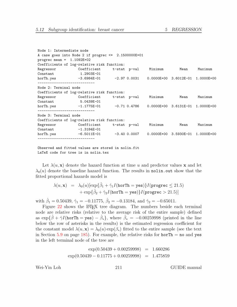
5.12 Subgroup identification: breast cancer 5 REGRESSION
Node 1: Intermediate node
A case goes into Node 2 if progrec <= 2.1500000E+01
progrec mean = 1.1092E+02
Coefficients of log-relative risk function:
Regressor Coefficient t-stat p-val Minimum Mean Maximum
Constant 1.2903E-01
horTh.yes -3.6984E-01 -2.97 0.0031 0.0000E+00 3.6012E-01 1.0000E+00
----------------------------
Node 2: Terminal node
Coefficients of log-relative risk function:
Regressor Coefficient t-stat p-val Minimum Mean Maximum
Constant 5.0439E-01
horTh.yes -1.1775E-01 -0.71 0.4786 0.0000E+00 3.6131E-01 1.0000E+00
----------------------------
Node 3: Terminal node
Coefficients of log-relative risk function:
Regressor Coefficient t-stat p-val Minimum Mean Maximum
Constant -1.3184E-01
horTh.yes -6.5011E-01 -3.40 0.0007 0.0000E+00 3.5930E-01 1.0000E+00
----------------------------
Observed and fitted values are stored in nolin.fit
LaTeX code for tree is in nolin.tex
Let λ(u,x) denote the hazard function at time u and predictor values x and letλ0(u) denote the baseline hazard function. The results in nolin.out show that thefitted proportional hazards model is
λ(u,x) = λ0(u)[exp{β1 + γ1I(horTh = yes)}I(progrec ≤ 21.5)
+ exp{β2 + γ2I(horTh = yes)}I(progrec > 21.5)]
with β1 = 0.50439, γ1 = −0.11775, β2 = −0.13184, and γ2 = −0.65011.Figure 22 shows the LATEX tree diagram. The numbers beside each terminal
node are relative risks (relative to the average risk of the entire sample) definedas exp{β + γI(horTh = yes) − β∗}, where β∗ = −0.00259998 (printed in the linebelow the row of asterisks in the results) is the estimated regression coefficient forthe constant model λ(u,x) = λ0(u) exp(β∗) fitted to the entire sample (see the textin Section 5.9 on page 185). For example, the relative risks for horTh = no and yes
in the left terminal node of the tree are
exp(0.50439 + 0.00259998) = 1.660286
exp(0.50439− 0.11775 + 0.00259998) = 1.475859
Wei-Yin Loh 211 GUIDE manual

5.12 Subgroup identification: breast cancer 5 REGRESSION
progrec≤ 21.50 1
1.6601.476 2
274
3
398
0.8790.459
Figure 22: GUIDE v.27.9 0.25-SE Gi proportional hazards regression tree for differ-ential treatment effects for time without linear prognostic effects. Maximum numberof split levels is 10, minimum node sample size is 33 and minimum number per treat-ment level is 2. At each split, an observation goes to the left branch if and only ifthe condition is satisfied. Numbers beside terminal nodes are estimated relative risks(relative to average for sample ignoring covariates) corresponding to horTh levels noand yes, respectively; numbers (in italics) below are sample sizes. Nodes with neg-ative and positive effects for horTh level yes are colored red and green, respectively.Second best split variable at root node is estrec.
500 1000 2000
0.0
0.4
0.8
Sur
viva
l pro
babi
lity
Node 2
horTh = yeshorTh = no
500 1000 2000
0.0
0.4
0.8
Node 3
horTh = yeshorTh = no
Figure 23: Estimated survival probability functions for breast cancer data
Wei-Yin Loh 212 GUIDE manual

5.12 Subgroup identification: breast cancer 5 REGRESSION
respectively. The Kaplan-Meier survival functions estimated from the data in theterminal nodes of the tree are shown in Figure 23. The plots are produced by thefollowing R code.
library(survival)
z <- read.table("cancer.dat",header=FALSE)
names(z) <- c("horTh","age","menostat","tsize","tgrade","pnodes","progrec",
"estrec","time","death")
leg.txt <- c("horTh = yes","horTh = no")
leg.col <- c("red","blue")
leg.lty <- 1:2
xr <- range(z$time)
zg <- read.table("nolin.fit",header=TRUE)
nodes <- zg$node
uniq.gp <- unique(sort(nodes))
plotted <- FALSE
for(g in uniq.gp){
gp <- nodes == g
y <- z$time[gp]
stat <- z$death[gp]
treat <- z$horTh[gp]
fit <- survfit(Surv(y,stat) ~ treat, conf.type="none")
if(plotted){
plot(fit,xlim=xr,mark.time=FALSE,xlab="",ylab="",col=c("blue","red"),lwd=2)
} else {
plot(fit,xlim=xr,mark.time=FALSE,xlab="",ylab="Survival probability",
col=c("blue","red"),lwd=2)
plotted <- TRUE
}
title(paste("Node",g))
legend("bottomleft",legend=leg.txt,lty=1,col=leg.col,lwd=2)
}
Estimated relative risks and survival probabilities The file nolin.fit givesthe terminal node number, estimated survival time, log baseline cumulative haz-ard, relative risk (relative to the average for the data, ignoring covariates), survivalprobability, and median survival time of each observation in the training sample filecancer.txt. The results for the first few observations are shown below. A plus (+)sign at the end of a value in the last column indicates that the observed survivaltime is censored. See Section 5.9 for definitions of the terms.
train node survivaltime logbasecumhaz relativerisk survivalprob mediansurvtime
y 3 1.814000E+03 -3.317667E-01 8.787636E-01 5.331186E-01 2.014420E+03
y 3 2.018000E+03 -2.024282E-01 4.587030E-01 6.882035E-01 2.659000E+03+
y 3 7.120000E+02 -1.300331E+00 4.587030E-01 8.828100E-01 2.659000E+03+
Wei-Yin Loh 213 GUIDE manual

5.12 Subgroup identification: breast cancer 5 REGRESSION
y 3 1.807000E+03 -3.550694E-01 4.587030E-01 7.255880E-01 2.659000E+03+
y 3 7.720000E+02 -1.176558E+00 8.787636E-01 7.631865E-01 2.014420E+03
y 2 4.480000E+02 -2.105688E+00 1.660293E+00 8.173929E-01 1.038277E+03
5.12.2 Simple linear prognostic control
To reduce or eliminate confounding between treatment and covariate variables, itmay be desirable to adjust for the effects of the latter by fitting a regression modelthat allows for thr linear effects of one or more prognostic variables in each node.This is done by choosing the “simple linear” or the “multiple linear” option andspecifying each potential linear predictor as “n” in the description file (no change isneeded in cancerdsc.txt). First we show how to choose the simple linear option,where a single prognostic variable is used in each node.
Input file generation
0. Read the warranty disclaimer
1. Create a GUIDE input file
Input your choice: 1
Name of batch input file: lin.in
Input 1 for model fitting, 2 for importance or DIF scoring,
3 for data conversion ([1:3], <cr>=1):
Name of batch output file: lin.out
Input 1 for single tree, 2 for ensemble ([1:2], <cr>=1):
Input 1 for classification, 2 for regression, 3 for propensity score grouping
(propensity score grouping is an experimental option)
Input your choice ([1:3], <cr>=1): 2
Choose type of regression model:
1=linear, 2=quantile, 3=Poisson, 4=proportional hazards,
5=multiresponse or itemresponse, 6=longitudinal data (with T variables).
Input choice ([1:6], <cr>=1): 4
Choose complexity of model to use at each node:
Choose 1 for multiple regression (recommended if R variable is present,
unless there are too many N, F or B variables)
Choose 2 for simple linear in one N or F variable + R (if present)
Choose 3 to fit a constant + R (if present)
1: multiple linear, 2: simple linear, 3: constant ([1:3], <cr>=3): 2
Option 2 fits one prognostic variable in each node.
Input 1 for default options, 2 otherwise ([1:2], <cr>=1):
Input name of data description file (max 100 characters);
enclose with matching quotes if it has spaces: cancerdsc.txt
Reading data description file ...
Wei-Yin Loh 214 GUIDE manual

5.12 Subgroup identification: breast cancer 5 REGRESSION
Training sample file: cancer.txt
Missing value code: NA
Records in data file start on line 1
R variable present
Dependent variable is death
Reading data file ...
Number of records in data file: 686
Length of longest entry in data file: 4
Checking for missing values ...
Total number of cases: 686
Col. no. Categorical variable #levels #missing values
1 horTh 2 0
3 menostat 2 0
Treatment (R) variable is horTh with values "no" and "yes"
Re-checking data ...
Assigning codes to categorical and missing values
Data checks complete
Smallest uncensored T: 72.00
No. cases dropped due to missing D or T or censored T < smallest uncensored T: 14
No. complete cases excluding censored T < smallest uncensored T: 672
No. cases used to compute baseline hazard: 672
No. cases with D=1 and T >= smallest uncensored: 299
GUIDE will try to create the variables in the description file.
If it is unsuccessful, please create the columns yourself...
Number of dummy variables created: 1
Choose a subgroup identification method:
1 = Sum of chi-squares (Gs)
2 = Treatment interactions (Gi)
Input your choice: ([1:2], <cr>=2):
Creating dummy variables
Rereading data
Total #cases w/ #missing
#cases miss. D ord. vals #X-var #N-var #F-var #S-var #B-var #C-var #R-var
686 0 0 0 6 0 0 0 1 1
Survival time variable in column: 9
Event indicator variable in column: 10
Proportion uncensored among nonmissing T and D variables: .445
No. cases used for training: 672
Finished reading data file
Input 1 for LaTeX tree code, 2 to skip it ([1:2], <cr>=1):
Input file name to store LaTeX code (use .tex as suffix): lin.tex
Input 2 to save fitted values and node IDs, 1 otherwise ([1:2], <cr>=2):
Input name of file to store node ID and fitted value of each case: lin.fit
Input 2 to write R function for predicting new cases, 1 otherwise ([1:2], <cr>=1):
Input file is created!
Run GUIDE with the command: guide < lin.in
Wei-Yin Loh 215 GUIDE manual

5.12 Subgroup identification: breast cancer 5 REGRESSION
Results The results in the following output file lin.out show that there are nosplits. The best linear predictor at the root node is the prognostic variable pnodes.
Proportional hazards regression with relative risk estimates
No truncation of predicted values
Pruning by cross-validation
Data description file: cancerdsc.txt
Training sample file: cancer.txt
Missing value code: NA
Records in data file start on line 1
R variable present
Dependent variable is death
Piecewise simple linear or constant model
Powers are dropped if they are not significant at level 1.0000
Number of records in data file: 686
Length of longest entry in data file: 4
Treatment (R) variable is horTh with values "no" and "yes"
Smallest uncensored T: 72.00
No. cases dropped due to missing D or T or censored T < smallest uncensored T: 14
No. complete cases excluding censored T < smallest uncensored T: 672
No. cases used to compute baseline hazard: 672
No. cases with D=1 and T >= smallest uncensored: 299
Number of dummy variables created: 1
Summary information (without x variables)
d=dependent, b=split and fit cat variable using 0-1 dummies,
c=split-only categorical, n=split and fit numerical, f=fit-only numerical,
s=split-only numerical, w=weight
t=survival time variable
Column Name Minimum Maximum #Categories #Missing
1 horTh r 2
2 age n 2.1000E+01 8.0000E+01
3 menostat c 2
4 tsize n 3.0000E+00 1.2000E+02
5 tgrade n 1.0000E+00 3.0000E+00
6 pnodes n 1.0000E+00 5.1000E+01
7 progrec n 0.0000E+00 2.3800E+03
8 estrec n 0.0000E+00 1.1440E+03
9 time t 7.2000E+01 2.6590E+03
10 death d 0.0000E+00 1.0000E+00
=================== Constructed variables ===================
11 lnbasehaz0 z -6.5103E+00 5.8866E-02
12 horTh.yes f 0.0000E+00 1.0000E+00
Wei-Yin Loh 216 GUIDE manual
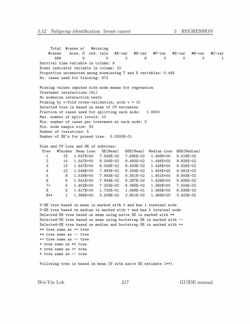
5.12 Subgroup identification: breast cancer 5 REGRESSION
Total #cases w/ #missing
#cases miss. D ord. vals #X-var #N-var #F-var #S-var #B-var #C-var
686 0 0 0 6 0 0 0 1
Survival time variable in column: 9
Event indicator variable in column: 10
Proportion uncensored among nonmissing T and D variables: 0.445
No. cases used for training: 672
Missing values imputed with node means for regression
Treatment interactions (Gi)
No nodewise interaction tests
Pruning by v-fold cross-validation, with v = 10
Selected tree is based on mean of CV estimates
Fraction of cases used for splitting each node: 1.0000
Max. number of split levels: 10
Min. number of cases per treatment at each node: 2
Min. node sample size: 33
Number of iterations: 5
Number of SE’s for pruned tree: 5.0000E-01
Size and CV Loss and SE of subtrees:
Tree #Tnodes Mean Loss SE(Mean) BSE(Mean) Median Loss BSE(Median)
1 15 1.537E+00 7.549E-02 7.695E-02 1.456E+00 9.019E-02
2 14 1.547E+00 8.006E-02 8.493E-02 1.446E+00 9.826E-02
3 13 1.547E+00 8.006E-02 8.493E-02 1.446E+00 9.826E-02
4 12 1.546E+00 7.983E-02 8.234E-02 1.453E+00 9.581E-02
5 8 1.539E+00 7.943E-02 8.351E-02 1.451E+00 9.693E-02
6 6 1.541E+00 7.944E-02 8.287E-02 1.434E+00 9.826E-02
7+ 5 1.452E+00 7.204E-02 6.366E-02 1.360E+00 7.504E-02
8 2 1.617E+00 1.720E-01 1.496E-01 1.465E+00 8.938E-02
9** 1 1.386E+00 5.508E-02 2.851E-02 1.366E+00 3.423E-02
0-SE tree based on mean is marked with * and has 1 terminal node
0-SE tree based on median is marked with + and has 5 terminal node
Selected-SE tree based on mean using naive SE is marked with **
Selected-SE tree based on mean using bootstrap SE is marked with --
Selected-SE tree based on median and bootstrap SE is marked with ++
** tree same as ++ tree
** tree same as -- tree
++ tree same as -- tree
* tree same as ** tree
* tree same as ++ tree
* tree same as -- tree
Following tree is based on mean CV with naive SE estimate (**).
Wei-Yin Loh 217 GUIDE manual

5.12 Subgroup identification: breast cancer 5 REGRESSION
Structure of final tree. Each terminal node is marked with a T.
Rel. risk is mean risk relative to sample average ignoring covariates
Cases fit give the number of cases used to fit node
Deviance is mean residual deviance for all cases in node
Node Total Cases Matrix Node Node Split
label cases fit rank rel.risk deviance variable
1T 672 672 3 1.000E+00 1.352E+00 estrec
Best split at root node is on estrec at 4.5000000000000000
Number of terminal nodes of final tree: 1
Total number of nodes of final tree: 1
Second best split variable (based on curvature test) at root node is progrec
Regression tree:
Node 1: Risk relative to sample average ignoring covariates = 1.00000
***************************************************************
Constant term for constant hazard model (ignoring covariates): -0.00462278
Node 1: Terminal node
Coefficients of log-relative risk function:
Regressor Coefficient t-stat p-val Minimum Mean Maximum
Constant -1.6815E-01
pnodes 5.7675E-02 8.82 0.0000 1.0000E+00 4.9866E+00 5.1000E+01
horTh.yes -3.5694E-01 -2.86 0.0044 0.0000E+00 3.6012E-01 1.0000E+00
----------------------------
Observed and fitted values are stored in lin.fit
LaTeX code for tree is in lin.tex
5.12.3 Multiple linear prognostic control
Now we show how to use all n variables as linear predictors in each node.
Input file generation
0. Read the warranty disclaimer
1. Create a GUIDE input file
Input your choice: 1
Wei-Yin Loh 218 GUIDE manual

5.12 Subgroup identification: breast cancer 5 REGRESSION
Name of batch input file: mul.in
Input 1 for model fitting, 2 for importance or DIF scoring,
3 for data conversion ([1:3], <cr>=1):
Name of batch output file: mul.out
Input 1 for single tree, 2 for ensemble ([1:2], <cr>=1):
Input 1 for classification, 2 for regression, 3 for propensity score grouping
(propensity score grouping is an experimental option)
Input your choice ([1:3], <cr>=1): 2
Choose type of regression model:
1=linear, 2=quantile, 3=Poisson, 4=proportional hazards,
5=multiresponse or itemresponse, 6=longitudinal data (with T variables).
Input choice ([1:6], <cr>=1): 4
Choose complexity of model to use at each node:
Choose 1 for multiple regression (recommended if R variable is present,
unless there are too many N, F or B variables)
Choose 2 for simple linear in one N or F variable + R (if present)
Choose 3 to fit a constant + R (if present)
1: multiple linear, 2: simple linear, 3: constant ([1:3], <cr>=3): 1
Input 1 for default options, 2 otherwise ([1:2], <cr>=1):
Option 1 fits all n and f variables in each node.
Input name of data description file (max 100 characters);
enclose with matching quotes if it has spaces: cancerdsc.txt
Reading data description file ...
Training sample file: cancer.txt
Missing value code: NA
Records in data file start on line 1
R variable present
Dependent variable is death
Reading data file ...
Number of records in data file: 686
Length of longest entry in data file: 4
Checking for missing values ...
Total number of cases: 686
Col. no. Categorical variable #levels #missing values
1 horTh 2 0
3 menostat 2 0
Treatment (R) variable is horTh with values "no" and "yes"
Re-checking data ...
Assigning codes to categorical and missing values
Data checks complete
Smallest uncensored T: 72.00
No. cases dropped due to missing D or T or censored T < smallest uncensored T: 14
No. complete cases excluding censored T < smallest uncensored T: 672
No. cases used to compute baseline hazard: 672
No. cases with D=1 and T >= smallest uncensored: 299
GUIDE will try to create the variables in the description file.
Wei-Yin Loh 219 GUIDE manual
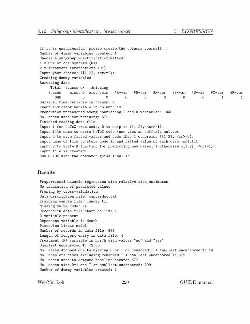
5.12 Subgroup identification: breast cancer 5 REGRESSION
If it is unsuccessful, please create the columns yourself...
Number of dummy variables created: 1
Choose a subgroup identification method:
1 = Sum of chi-squares (Gs)
2 = Treatment interactions (Gi)
Input your choice: ([1:2], <cr>=2):
Creating dummy variables
Rereading data
Total #cases w/ #missing
#cases miss. D ord. vals #X-var #N-var #F-var #S-var #B-var #C-var #R-var
686 0 0 0 6 0 0 0 1 1
Survival time variable in column: 9
Event indicator variable in column: 10
Proportion uncensored among nonmissing T and D variables: .445
No. cases used for training: 672
Finished reading data file
Input 1 for LaTeX tree code, 2 to skip it ([1:2], <cr>=1):
Input file name to store LaTeX code (use .tex as suffix): mul.tex
Input 2 to save fitted values and node IDs, 1 otherwise ([1:2], <cr>=2):
Input name of file to store node ID and fitted value of each case: mul.fit
Input 2 to write R function for predicting new cases, 1 otherwise ([1:2], <cr>=1):
Input file is created!
Run GUIDE with the command: guide < mul.in
Results
Proportional hazards regression with relative risk estimates
No truncation of predicted values
Pruning by cross-validation
Data description file: cancerdsc.txt
Training sample file: cancer.txt
Missing value code: NA
Records in data file start on line 1
R variable present
Dependent variable is death
Piecewise linear model
Number of records in data file: 686
Length of longest entry in data file: 4
Treatment (R) variable is horTh with values "no" and "yes"
Smallest uncensored T: 72.00
No. cases dropped due to missing D or T or censored T < smallest uncensored T: 14
No. complete cases excluding censored T < smallest uncensored T: 672
No. cases used to compute baseline hazard: 672
No. cases with D=1 and T >= smallest uncensored: 299
Number of dummy variables created: 1
Wei-Yin Loh 220 GUIDE manual
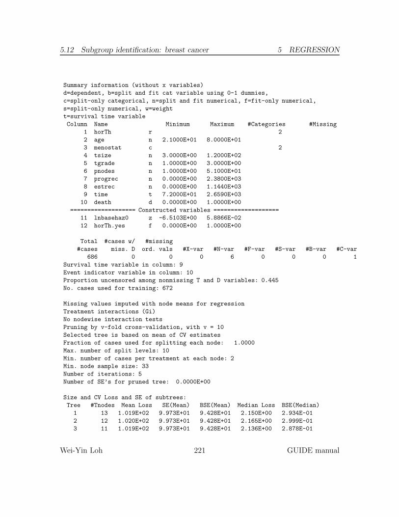
5.12 Subgroup identification: breast cancer 5 REGRESSION
Summary information (without x variables)
d=dependent, b=split and fit cat variable using 0-1 dummies,
c=split-only categorical, n=split and fit numerical, f=fit-only numerical,
s=split-only numerical, w=weight
t=survival time variable
Column Name Minimum Maximum #Categories #Missing
1 horTh r 2
2 age n 2.1000E+01 8.0000E+01
3 menostat c 2
4 tsize n 3.0000E+00 1.2000E+02
5 tgrade n 1.0000E+00 3.0000E+00
6 pnodes n 1.0000E+00 5.1000E+01
7 progrec n 0.0000E+00 2.3800E+03
8 estrec n 0.0000E+00 1.1440E+03
9 time t 7.2000E+01 2.6590E+03
10 death d 0.0000E+00 1.0000E+00
=================== Constructed variables ===================
11 lnbasehaz0 z -6.5103E+00 5.8866E-02
12 horTh.yes f 0.0000E+00 1.0000E+00
Total #cases w/ #missing
#cases miss. D ord. vals #X-var #N-var #F-var #S-var #B-var #C-var
686 0 0 0 6 0 0 0 1
Survival time variable in column: 9
Event indicator variable in column: 10
Proportion uncensored among nonmissing T and D variables: 0.445
No. cases used for training: 672
Missing values imputed with node means for regression
Treatment interactions (Gi)
No nodewise interaction tests
Pruning by v-fold cross-validation, with v = 10
Selected tree is based on mean of CV estimates
Fraction of cases used for splitting each node: 1.0000
Max. number of split levels: 10
Min. number of cases per treatment at each node: 2
Min. node sample size: 33
Number of iterations: 5
Number of SE’s for pruned tree: 0.0000E+00
Size and CV Loss and SE of subtrees:
Tree #Tnodes Mean Loss SE(Mean) BSE(Mean) Median Loss BSE(Median)
1 13 1.019E+02 9.973E+01 9.428E+01 2.150E+00 2.934E-01
2 12 1.020E+02 9.973E+01 9.428E+01 2.165E+00 2.999E-01
3 11 1.019E+02 9.973E+01 9.428E+01 2.136E+00 2.878E-01
Wei-Yin Loh 221 GUIDE manual

5.12 Subgroup identification: breast cancer 5 REGRESSION
4 10 1.019E+02 9.973E+01 9.428E+01 2.136E+00 2.863E-01
5 9 2.119E+00 1.641E-01 1.825E-01 1.920E+00 1.430E-01
6 7 1.963E+00 1.483E-01 1.068E-01 1.915E+00 1.539E-01
7 6 1.868E+00 1.429E-01 1.115E-01 1.859E+00 1.600E-01
8 5 1.817E+00 1.402E-01 1.202E-01 1.838E+00 1.829E-01
9** 1 1.363E+00 5.430E-02 3.322E-02 1.365E+00 4.288E-02
0-SE tree based on mean is marked with * and has 1 terminal node
0-SE tree based on median is marked with + and has 1 terminal node
Selected-SE tree based on mean using naive SE is marked with **
Selected-SE tree based on mean using bootstrap SE is marked with --
Selected-SE tree based on median and bootstrap SE is marked with ++
* tree, ** tree, + tree, and ++ tree all the same
Following tree is based on mean CV with naive SE estimate (**).
Structure of final tree. Each terminal node is marked with a T.
Rel. risk is mean risk relative to sample average ignoring covariates
Cases fit give the number of cases used to fit node
Deviance is mean residual deviance for all cases in node
Node Total Cases Matrix Node Node Split
label cases fit rank rel.risk deviance variable
1T 672 672 7 1.000E+00 1.322E+00 estrec
Best split at root node is on estrec at 1.5000000000000000
Number of terminal nodes of final tree: 1
Total number of nodes of final tree: 1
Second best split variable (based on curvature test) at root node is progrec
Regression tree:
Node 1: Risk relative to sample average ignoring covariates = 1.00000
***************************************************************
Constant term for constant hazard model (ignoring covariates): -0.01020401
Node 1: Terminal node
Coefficients of log-relative risk function:
Regressor Coefficient t-stat p-val Minimum Mean Maximum
Constant -8.0565E-01
age 6.1317E-04 0.10 0.9219 2.1000E+01 5.3077E+01 8.0000E+01
tsize 7.4417E-03 1.90 0.0579 3.0000E+00 2.9317E+01 1.2000E+02
Wei-Yin Loh 222 GUIDE manual

6 IMPORTANCE SCORING
tgrade 2.8302E-01 2.68 0.0075 1.0000E+00 2.1161E+00 3.0000E+00
pnodes 5.0016E-02 6.84 0.0000 1.0000E+00 4.9866E+00 5.1000E+01
progrec -2.3066E-03 -4.00 0.0001 0.0000E+00 1.1092E+02 2.3800E+03
estrec 1.7315E-04 0.39 0.6963 0.0000E+00 9.7475E+01 1.1440E+03
horTh.yes -3.2088E-01 -2.50 0.0126 0.0000E+00 3.6012E-01 1.0000E+00
----------------------------
Observed and fitted values are stored in mul.fit
LaTeX code for tree is in mul.tex
6 Importance scoring
When there are numerous predictor variables, it may be useful to rank them in orderof their “importance”. GUIDE has a facility to do this. In addition, it provides athreshold for distinguishing the important variables from the unimportant ones—seeLoh et al. (2015) and Loh (2012); the latter also shows that using GUIDE to find asubset of variables can increase the prediction accuracy of a model.
6.1 Classification: glaucoma data
6.1.1 Input file creation
0. Read the warranty disclaimer
1. Create a GUIDE input file
Input your choice: 1
Name of batch input file: imp.in
Input 1 for model fitting, 2 for importance or DIF scoring,
3 for data conversion ([1:3], <cr>=1): 2
Name of batch output file: imp.out
Input 1 for classification, 2 for regression, 3 for propensity score grouping
(propensity score grouping is an experimental option)
Input your choice ([1:3], <cr>=1):
Input 1 for default options, 2 otherwise ([1:2], <cr>=1):
Input name of data description file (max 100 characters);
enclose with matching quotes if it has spaces: glaucoma.dsc
Reading data description file ...
Training sample file: glaucoma.rdata
Missing value code: NA
Records in data file start on line 2
Warning: N variables changed to S
Dependent variable is Class
Wei-Yin Loh 223 GUIDE manual
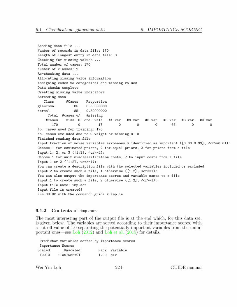
6.1 Classification: glaucoma data 6 IMPORTANCE SCORING
Reading data file ...
Number of records in data file: 170
Length of longest entry in data file: 8
Checking for missing values ...
Total number of cases: 170
Number of classes: 2
Re-checking data ...
Allocating missing value information
Assigning codes to categorical and missing values
Data checks complete
Creating missing value indicators
Rereading data
Class #Cases Proportion
glaucoma 85 0.50000000
normal 85 0.50000000
Total #cases w/ #missing
#cases miss. D ord. vals #X-var #N-var #F-var #S-var #B-var #C-var
170 0 17 0 0 0 66 0 0
No. cases used for training: 170
No. cases excluded due to 0 weight or missing D: 0
Finished reading data file
Input fraction of noise variables erroneously identified as important ([0.00:0.99], <cr>=0.01):
Choose 1 for estimated priors, 2 for equal priors, 3 for priors from a file
Input 1, 2, or 3 ([1:3], <cr>=2):
Choose 1 for unit misclassification costs, 2 to input costs from a file
Input 1 or 2 ([1:2], <cr>=1):
You can create a description file with the selected variables included or excluded
Input 2 to create such a file, 1 otherwise ([1:2], <cr>=1):
You can also output the importance scores and variable names to a file
Input 1 to create such a file, 2 otherwise ([1:2], <cr>=1):
Input file name: imp.scr
Input file is created!
Run GUIDE with the command: guide < imp.in
6.1.2 Contents of imp.out
The most interesting part of the output file is at the end which, for this data set,is given below. The variables are sorted according to their importance scores, witha cut-off value of 1.0 separating the potentially important variables from the unim-portant ones—see Loh (2012) and Loh et al. (2015) for details.
Predictor variables sorted by importance scores
Importance Scores
Scaled Unscaled Rank Variable
100.0 1.05708E+01 1.00 clv
Wei-Yin Loh 224 GUIDE manual
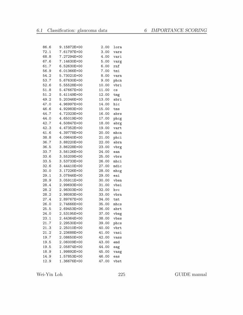
6.1 Classification: glaucoma data 6 IMPORTANCE SCORING
86.6 9.15872E+00 2.00 lora
72.1 7.61797E+00 3.00 vars
68.8 7.27294E+00 4.00 vari
67.6 7.14630E+00 5.00 varg
61.7 6.52630E+00 6.00 rnf
56.9 6.01366E+00 7.00 tmi
54.2 5.73021E+00 8.00 varn
53.7 5.67630E+00 9.00 phcn
52.6 5.55528E+00 10.00 vbri
51.8 5.47667E+00 11.00 cs
51.2 5.41149E+00 12.00 tmg
49.2 5.20346E+00 13.00 abri
47.0 4.96997E+00 14.00 hic
46.6 4.92983E+00 15.00 tms
44.7 4.72323E+00 16.00 abrs
44.0 4.65019E+00 17.00 phcg
42.7 4.50847E+00 18.00 abrg
42.3 4.47352E+00 19.00 vart
41.6 4.39778E+00 20.00 mhcn
38.8 4.09640E+00 21.00 phci
36.7 3.88220E+00 22.00 abrn
36.5 3.86228E+00 23.00 vbrg
33.7 3.56126E+00 24.00 ean
33.6 3.55209E+00 25.00 vbrs
33.5 3.53733E+00 26.00 mhci
32.6 3.44410E+00 27.00 mdic
30.0 3.17226E+00 28.00 mhcg
29.1 3.07846E+00 29.00 eai
28.9 3.05911E+00 30.00 vbsn
28.4 2.99693E+00 31.00 vbsi
28.2 2.98303E+00 32.00 hvc
28.2 2.98083E+00 33.00 vbrn
27.4 2.89767E+00 34.00 tmt
26.0 2.74666E+00 35.00 mhcs
25.5 2.69453E+00 36.00 abrt
24.0 2.53195E+00 37.00 vbsg
23.1 2.44364E+00 38.00 vbss
21.7 2.29530E+00 39.00 phcs
21.3 2.25010E+00 40.00 vbrt
21.2 2.23688E+00 41.00 vasi
19.7 2.08650E+00 42.00 vass
19.5 2.06009E+00 43.00 emd
19.5 2.05874E+00 44.00 eag
18.9 1.99892E+00 45.00 vasg
14.9 1.57853E+00 46.00 eas
12.9 1.36676E+00 47.00 vbst
Wei-Yin Loh 225 GUIDE manual
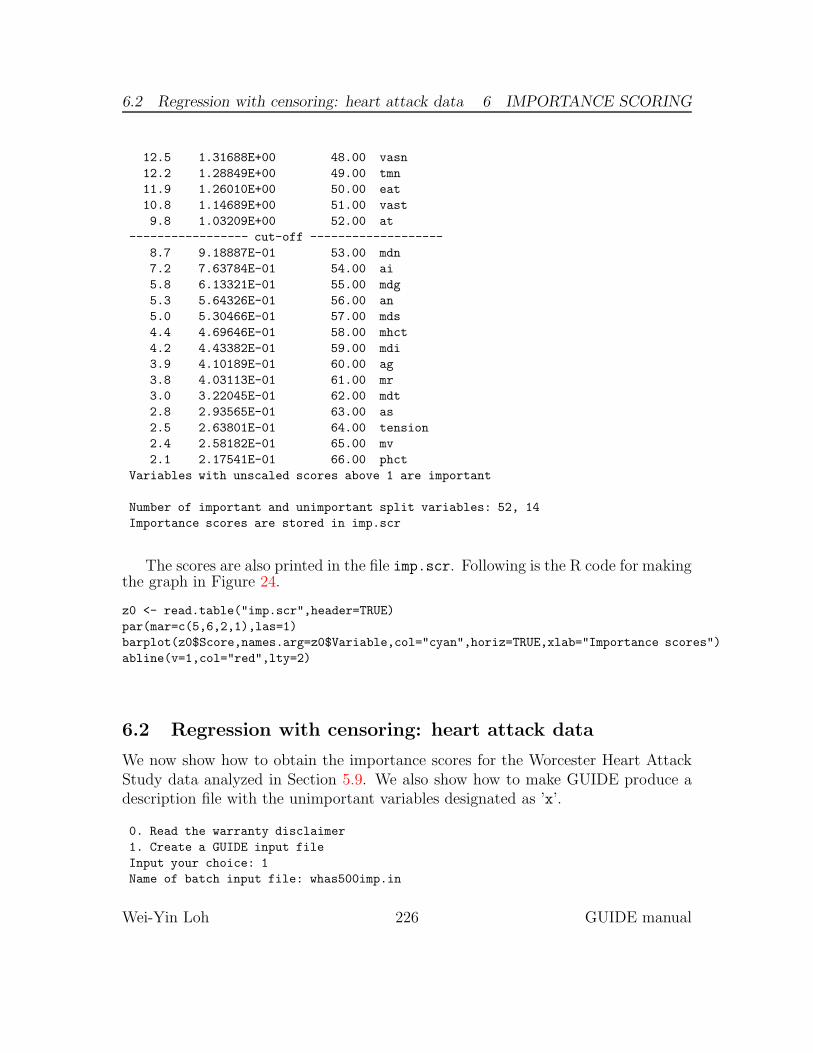
6.2 Regression with censoring: heart attack data 6 IMPORTANCE SCORING
12.5 1.31688E+00 48.00 vasn
12.2 1.28849E+00 49.00 tmn
11.9 1.26010E+00 50.00 eat
10.8 1.14689E+00 51.00 vast
9.8 1.03209E+00 52.00 at
----------------- cut-off -------------------
8.7 9.18887E-01 53.00 mdn
7.2 7.63784E-01 54.00 ai
5.8 6.13321E-01 55.00 mdg
5.3 5.64326E-01 56.00 an
5.0 5.30466E-01 57.00 mds
4.4 4.69646E-01 58.00 mhct
4.2 4.43382E-01 59.00 mdi
3.9 4.10189E-01 60.00 ag
3.8 4.03113E-01 61.00 mr
3.0 3.22045E-01 62.00 mdt
2.8 2.93565E-01 63.00 as
2.5 2.63801E-01 64.00 tension
2.4 2.58182E-01 65.00 mv
2.1 2.17541E-01 66.00 phct
Variables with unscaled scores above 1 are important
Number of important and unimportant split variables: 52, 14
Importance scores are stored in imp.scr
The scores are also printed in the file imp.scr. Following is the R code for makingthe graph in Figure 24.
z0 <- read.table("imp.scr",header=TRUE)
par(mar=c(5,6,2,1),las=1)
barplot(z0$Score,names.arg=z0$Variable,col="cyan",horiz=TRUE,xlab="Importance scores")
abline(v=1,col="red",lty=2)
6.2 Regression with censoring: heart attack data
We now show how to obtain the importance scores for the Worcester Heart AttackStudy data analyzed in Section 5.9. We also show how to make GUIDE produce adescription file with the unimportant variables designated as ’x’.
0. Read the warranty disclaimer
1. Create a GUIDE input file
Input your choice: 1
Name of batch input file: whas500imp.in
Wei-Yin Loh 226 GUIDE manual
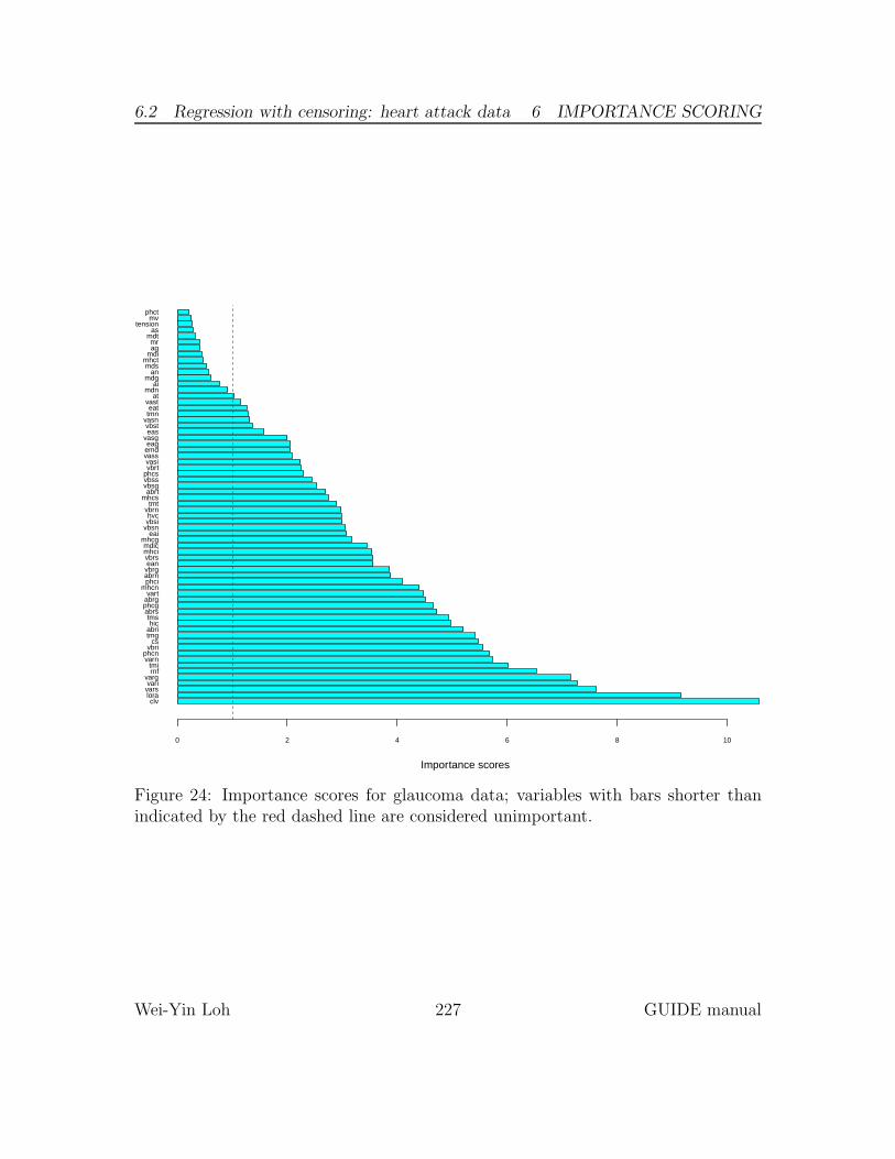
6.2 Regression with censoring: heart attack data 6 IMPORTANCE SCORING
clvloravarsvari
vargrnftmi
varnphcn
vbrics
tmgabrihic
tmsabrsphcgabrgvart
mhcnphciabrnvbrgeanvbrsmhcimdic
mhcgeai
vbsnvbsihvc
vbrntmt
mhcsabrt
vbsgvbssphcsvbrtvasi
vassemdeag
vasgeasvbst
vasntmneat
vastat
mdnai
mdgan
mdsmhctmdiagmr
mdtas
tensionmv
phct
Importance scores
0 2 4 6 8 10
Figure 24: Importance scores for glaucoma data; variables with bars shorter thanindicated by the red dashed line are considered unimportant.
Wei-Yin Loh 227 GUIDE manual
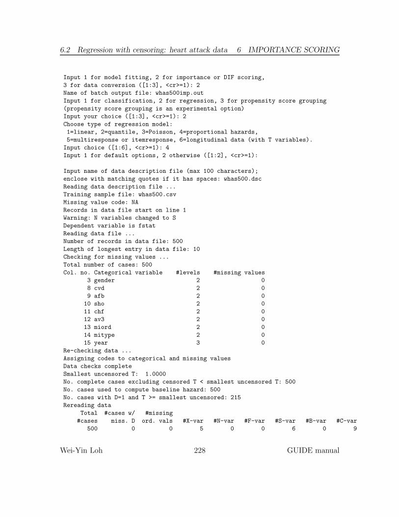
6.2 Regression with censoring: heart attack data 6 IMPORTANCE SCORING
Input 1 for model fitting, 2 for importance or DIF scoring,
3 for data conversion ([1:3], <cr>=1): 2
Name of batch output file: whas500imp.out
Input 1 for classification, 2 for regression, 3 for propensity score grouping
(propensity score grouping is an experimental option)
Input your choice ([1:3], <cr>=1): 2
Choose type of regression model:
1=linear, 2=quantile, 3=Poisson, 4=proportional hazards,
5=multiresponse or itemresponse, 6=longitudinal data (with T variables).
Input choice ([1:6], <cr>=1): 4
Input 1 for default options, 2 otherwise ([1:2], <cr>=1):
Input name of data description file (max 100 characters);
enclose with matching quotes if it has spaces: whas500.dsc
Reading data description file ...
Training sample file: whas500.csv
Missing value code: NA
Records in data file start on line 1
Warning: N variables changed to S
Dependent variable is fstat
Reading data file ...
Number of records in data file: 500
Length of longest entry in data file: 10
Checking for missing values ...
Total number of cases: 500
Col. no. Categorical variable #levels #missing values
3 gender 2 0
8 cvd 2 0
9 afb 2 0
10 sho 2 0
11 chf 2 0
12 av3 2 0
13 miord 2 0
14 mitype 2 0
15 year 3 0
Re-checking data ...
Assigning codes to categorical and missing values
Data checks complete
Smallest uncensored T: 1.0000
No. complete cases excluding censored T < smallest uncensored T: 500
No. cases used to compute baseline hazard: 500
No. cases with D=1 and T >= smallest uncensored: 215
Rereading data
Total #cases w/ #missing
#cases miss. D ord. vals #X-var #N-var #F-var #S-var #B-var #C-var
500 0 0 5 0 0 6 0 9
Wei-Yin Loh 228 GUIDE manual

6.2 Regression with censoring: heart attack data 6 IMPORTANCE SCORING
Survival time variable in column: 21
Event indicator variable in column: 22
Proportion uncensored among nonmissing T and D variables: .430
No. cases used for training: 500
Finished reading data file
Input fraction of noise variables erroneously identified as important ([0.00:0.99], <cr>=0.01):
You can create a description file with the selected variables included or excluded
Input 2 to create such a file, 1 otherwise ([1:2], <cr>=1): 2
Input 1 to keep only selected variables, 2 to exclude selected variables ([1:2], <cr>=1):
This option produces a description file with unimportant variables marked as ’x’.
Input file name: whas500new.dsc
You can also output the importance scores and variable names to a file
Input 1 to create such a file, 2 otherwise ([1:2], <cr>=1):
Input file name: whas500imp.scr
Input file is created!
Run GUIDE with the command: guide < whas500imp.in
Results The importance scores are given at the end of the output file imp.out.Variables with scores below 1.0 (i.e., below the cut-off line) are considered unimpor-tant.
Proportional hazards regression with relative risk estimates
No pruning
Data description file: whas500.dsc
Training sample file: whas500.csv
Missing value code: NA
Records in data file start on line 1
Warning: N variables changed to S
Dependent variable is fstat
Piecewise constant model
Number of records in data file: 500
Length of longest entry in data file: 10
Smallest uncensored T: 1.0000
No. complete cases excluding censored T < smallest uncensored T: 500
No. cases used to compute baseline hazard: 500
No. cases with D=1 and T >= smallest uncensored: 215
Total #cases w/ #missing
#cases miss. D ord. vals #X-var #N-var #F-var #S-var #B-var #C-var
500 0 0 5 0 0 6 0 9
Survival time variable in column: 21
Event indicator variable in column: 22
Proportion uncensored among nonmissing T and D variables: 0.430
No. cases used for training: 500
Wei-Yin Loh 229 GUIDE manual
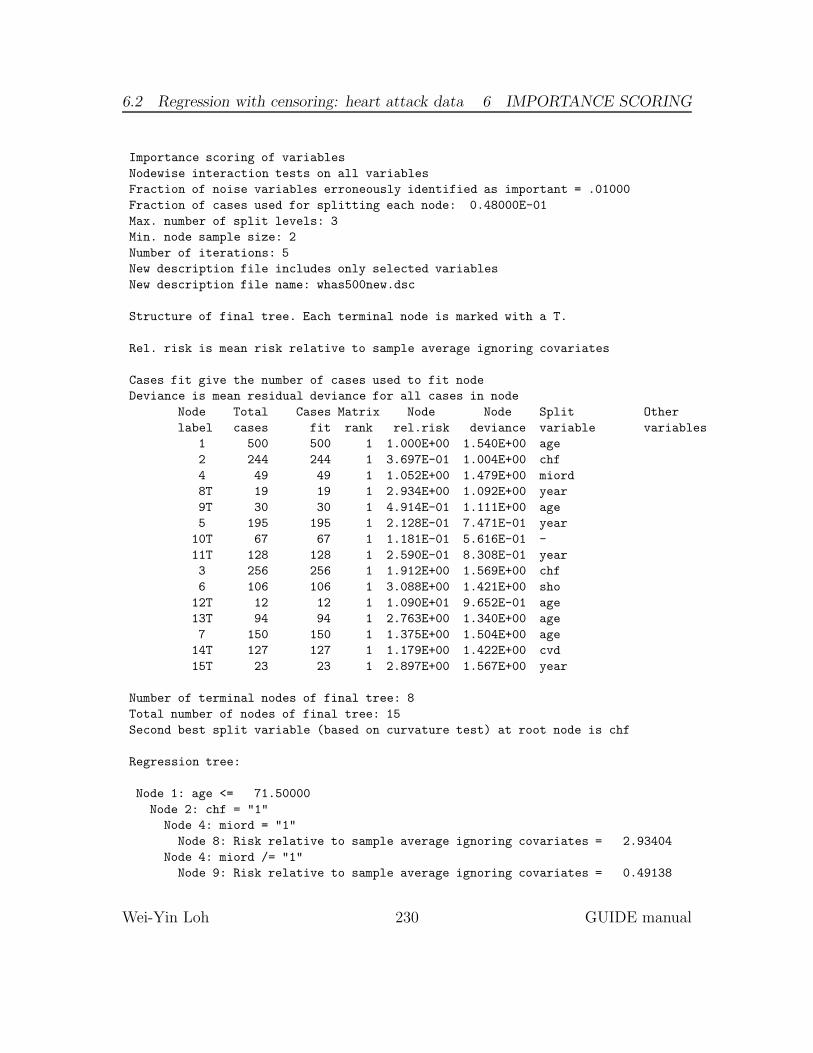
6.2 Regression with censoring: heart attack data 6 IMPORTANCE SCORING
Importance scoring of variables
Nodewise interaction tests on all variables
Fraction of noise variables erroneously identified as important = .01000
Fraction of cases used for splitting each node: 0.48000E-01
Max. number of split levels: 3
Min. node sample size: 2
Number of iterations: 5
New description file includes only selected variables
New description file name: whas500new.dsc
Structure of final tree. Each terminal node is marked with a T.
Rel. risk is mean risk relative to sample average ignoring covariates
Cases fit give the number of cases used to fit node
Deviance is mean residual deviance for all cases in node
Node Total Cases Matrix Node Node Split Other
label cases fit rank rel.risk deviance variable variables
1 500 500 1 1.000E+00 1.540E+00 age
2 244 244 1 3.697E-01 1.004E+00 chf
4 49 49 1 1.052E+00 1.479E+00 miord
8T 19 19 1 2.934E+00 1.092E+00 year
9T 30 30 1 4.914E-01 1.111E+00 age
5 195 195 1 2.128E-01 7.471E-01 year
10T 67 67 1 1.181E-01 5.616E-01 -
11T 128 128 1 2.590E-01 8.308E-01 year
3 256 256 1 1.912E+00 1.569E+00 chf
6 106 106 1 3.088E+00 1.421E+00 sho
12T 12 12 1 1.090E+01 9.652E-01 age
13T 94 94 1 2.763E+00 1.340E+00 age
7 150 150 1 1.375E+00 1.504E+00 age
14T 127 127 1 1.179E+00 1.422E+00 cvd
15T 23 23 1 2.897E+00 1.567E+00 year
Number of terminal nodes of final tree: 8
Total number of nodes of final tree: 15
Second best split variable (based on curvature test) at root node is chf
Regression tree:
Node 1: age <= 71.50000
Node 2: chf = "1"
Node 4: miord = "1"
Node 8: Risk relative to sample average ignoring covariates = 2.93404
Node 4: miord /= "1"
Node 9: Risk relative to sample average ignoring covariates = 0.49138
Wei-Yin Loh 230 GUIDE manual

6.2 Regression with censoring: heart attack data 6 IMPORTANCE SCORING
Node 2: chf /= "1"
Node 5: year = "2"
Node 10: Risk relative to sample average ignoring covariates = 0.11813
Node 5: year /= "2"
Node 11: Risk relative to sample average ignoring covariates = 0.25898
Node 1: age > 71.50000 or NA
Node 3: chf = "1"
Node 6: sho = "1"
Node 12: Risk relative to sample average ignoring covariates = 10.89637
Node 6: sho /= "1"
Node 13: Risk relative to sample average ignoring covariates = 2.76262
Node 3: chf /= "1"
Node 7: age <= 86.50000 or NA
Node 14: Risk relative to sample average ignoring covariates = 1.17892
Node 7: age > 86.50000
Node 15: Risk relative to sample average ignoring covariates = 2.89698
***************************************************************
WARNING: p-values below are not adjusted for split search. For a bootstrap
solution, see Loh et al. (2016), "Identification of subgroups with
differential treatment effects for longitudinal and multiresponse
variables", Statistics in Medicine, v.35, 4837-4855.
Node 1: Intermediate node
A case goes into Node 2 if age <= 7.1500000E+01
age mean = 6.9846E+01
Coefficients of log-relative risk function:
Regressor Coefficient t-stat p-val
Constant -4.7242E-02
Predicted relative risk = 1.0000000000000000
----------------------------
Node 2: Intermediate node
A case goes into Node 4 if chf = "1"
chf mode = "0"
----------------------------
Node 4: Intermediate node
A case goes into Node 8 if miord = "1"
miord mode = "0"
----------------------------
Node 8: Terminal node
Coefficients of log-relative risk function:
Regressor Coefficient t-stat p-val
Constant 1.0291E+00
Predicted relative risk = 2.9340385978987165
Wei-Yin Loh 231 GUIDE manual

6.2 Regression with censoring: heart attack data 6 IMPORTANCE SCORING
----------------------------
Node 9: Terminal node
Coefficients of log-relative risk function:
Regressor Coefficient t-stat p-val
Constant -7.5779E-01
Predicted relative risk = 0.49137683168653684
----------------------------
Node 5: Intermediate node
A case goes into Node 10 if year = "2"
year mode = "2"
----------------------------
Node 10: Terminal node
Coefficients of log-relative risk function:
Regressor Coefficient t-stat p-val
Constant -2.1832E+00
Predicted relative risk = 0.11813174498787163
----------------------------
Node 11: Terminal node
Coefficients of log-relative risk function:
Regressor Coefficient t-stat p-val
Constant -1.3982E+00
Predicted relative risk = 0.25898393382449247
----------------------------
Node 3: Intermediate node
A case goes into Node 6 if chf = "1"
chf mode = "0"
----------------------------
Node 6: Intermediate node
A case goes into Node 12 if sho = "1"
sho mode = "0"
----------------------------
Node 12: Terminal node
Coefficients of log-relative risk function:
Regressor Coefficient t-stat p-val
Constant 2.3412E+00
Predicted relative risk = 10.896372134501140
----------------------------
Node 13: Terminal node
Coefficients of log-relative risk function:
Regressor Coefficient t-stat p-val
Constant 9.6894E-01
Predicted relative risk = 2.7626196234631277
----------------------------
Node 7: Intermediate node
A case goes into Node 14 if age <= 8.6500000E+01 or NA
age mean = 8.0667E+01
Wei-Yin Loh 232 GUIDE manual

6.2 Regression with censoring: heart attack data 6 IMPORTANCE SCORING
----------------------------
Node 14: Terminal node
Coefficients of log-relative risk function:
Regressor Coefficient t-stat p-val
Constant 1.1736E-01
Predicted relative risk = 1.1789191007956614
----------------------------
Node 15: Terminal node
Coefficients of log-relative risk function:
Regressor Coefficient t-stat p-val
Constant 1.0164E+00
Predicted relative risk = 2.8969795749640870
----------------------------
******************************************************
Variables used for splitting or fitting:
age
chf
miord
sho
year
Number of terminal nodes: 8
Predictor variables sorted by importance scores
Importance Scores
Scaled Unscaled Rank Variable
100.0 1.23414E+01 1.00 age
83.5 1.03056E+01 2.00 chf
52.5 6.48506E+00 3.00 year
38.6 4.76455E+00 4.00 bmi
35.7 4.41122E+00 5.00 hr
23.7 2.92057E+00 6.00 diasbp
20.2 2.49131E+00 7.00 mitype
15.2 1.87900E+00 8.00 miord
14.2 1.74955E+00 9.00 sho
13.8 1.70162E+00 10.00 gender
13.4 1.64965E+00 11.00 afb
11.2 1.37849E+00 12.00 los
9.6 1.18834E+00 13.00 sysbp
----------------- cut-off -------------------
7.0 8.60112E-01 14.00 cvd
2.3 2.89589E-01 15.00 av3
Variables with unscaled scores above 1 are important
Number of important and unimportant split variables: 13, 2
Wei-Yin Loh 233 GUIDE manual

6.2 Regression with censoring: heart attack data 6 IMPORTANCE SCORING
Score scale for categorical variables with 2 and 3 levels = 1.100
Importance scores are stored in whas500imp.scr
Description file with selected variables in whas500new.dsc
The scores are also contained in the file whas500imp.scr for input into anothercomputer program:
Rank Score Variable
1.00 1.23414E+01 age
2.00 1.03056E+01 chf
3.00 6.48506E+00 year
4.00 4.76455E+00 bmi
5.00 4.41122E+00 hr
6.00 2.92057E+00 diasbp
7.00 2.49131E+00 mitype
8.00 1.87900E+00 miord
9.00 1.74955E+00 sho
10.00 1.70162E+00 gender
11.00 1.64965E+00 afb
12.00 1.37849E+00 los
13.00 1.18834E+00 sysbp
14.00 8.60112E-01 cvd
15.00 2.89589E-01 av3
Finally, here are the contents of the file whas500new.dsc. It puts an “x” againstthe variables (cvd and av3 here) that are not important.
"whas500.csv"
"NA"
1
1 id x
2 age n
3 gender c
4 hr n
5 sysbp n
6 diasbp n
7 bmi n
8 cvd x
9 afb c
10 sho c
11 chf c
12 av3 x
13 miord c
14 mitype c
15 year c
Wei-Yin Loh 234 GUIDE manual

7 DIFFERENTIAL ITEM FUNCTIONING: GDS DATA
16 admitdate x
17 disdate x
18 fdate x
19 los n
20 dstat x
21 lenfol t
22 fstat d
7 Differential item functioning: GDS data
GUIDE has an experimental option to identify important predictor variables anditems with differential item functioning (DIF) in a data set with two or more item(dependent variable) scores. We illustrate it with a data set from Broekman et al.(2011, 2008) and Marc et al. (2008). It consists of responses from 1978 subjects on15 items. There are 3 predictor variables (age, education, and gender). The dataand description files are GDS.dat and GDS.dsc. Although the item responses in thisexample are 0-1, GUIDE allows them to be in any ordinal (e.g., Likert) scale. Thecontents of GDS.dsc are:
GDS.dat
NA
1
1 rid x
2 satis d
3 drop d
4 empty d
5 bored d
6 spirit d
7 afraid d
8 happy d
9 help d
10 home d
11 memory d
12 alive d
13 worth d
14 energy d
15 hope d
16 better d
17 total x
18 gender c
19 education n
20 age n
21 dxcurren x
22 sumscore x
Wei-Yin Loh 235 GUIDE manual
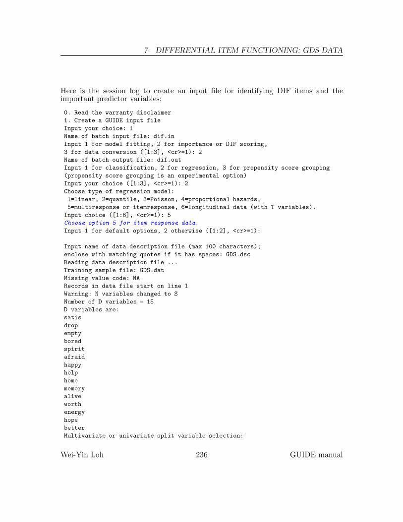
7 DIFFERENTIAL ITEM FUNCTIONING: GDS DATA
Here is the session log to create an input file for identifying DIF items and theimportant predictor variables:
0. Read the warranty disclaimer
1. Create a GUIDE input file
Input your choice: 1
Name of batch input file: dif.in
Input 1 for model fitting, 2 for importance or DIF scoring,
3 for data conversion ([1:3], <cr>=1): 2
Name of batch output file: dif.out
Input 1 for classification, 2 for regression, 3 for propensity score grouping
(propensity score grouping is an experimental option)
Input your choice ([1:3], <cr>=1): 2
Choose type of regression model:
1=linear, 2=quantile, 3=Poisson, 4=proportional hazards,
5=multiresponse or itemresponse, 6=longitudinal data (with T variables).
Input choice ([1:6], <cr>=1): 5
Choose option 5 for item response data.
Input 1 for default options, 2 otherwise ([1:2], <cr>=1):
Input name of data description file (max 100 characters);
enclose with matching quotes if it has spaces: GDS.dsc
Reading data description file ...
Training sample file: GDS.dat
Missing value code: NA
Records in data file start on line 1
Warning: N variables changed to S
Number of D variables = 15
D variables are:
satis
drop
empty
bored
spirit
afraid
happy
help
home
memory
alive
worth
energy
hope
better
Multivariate or univariate split variable selection:
Wei-Yin Loh 236 GUIDE manual

7 DIFFERENTIAL ITEM FUNCTIONING: GDS DATA
Choose multivariate if there is an order among the D variables; otherwise choose univariate
Input 1 for multivariate, 2 for univariate ([1:2], <cr>=1): 2
Input 1 to normalize D variables, 2 for no normalization ([1:2], <cr>=1): 2
Input 1 for equal, 2 for unequal weighting of D variables ([1:2], <cr>=1):
Reading data file ...
Number of records in data file: 989
Length of longest entry in data file: 4
Checking for missing values ...
Total number of cases: 989
Col. no. Categorical variable #levels #missing values
18 gender 2 0
Re-checking data ...
Allocating missing value information
Assigning codes to categorical and missing values
Data checks complete
Creating missing value indicators
Some D variables have missing values
You can use all the data or only those with complete D values
Using only cases with complete D values will reduce the sample size
but allows the option of using PCA for split selection
Input 1 to use all obs, 2 to use obs with complete D values ([1:2], <cr>=2):
Rereading data
PCA can be used for variable selection
Do not use PCA if differential item functioning (DIF) scores are wanted
Input 1 to use PCA, 2 otherwise ([1:2], <cr>=2):
Choose option 2 because DIF scoring is desired.
#cases w/ miss. D = number of cases with all D values missing
Total #cases w/ #missing
#cases miss. D ord. vals #X-var #N-var #F-var #S-var #B-var #C-var
989 0 0 4 0 0 2 0 1
No. cases used for training: 988
No. cases excluded due to 0 weight or missing D: 1
Finished reading data file
Warning: interaction tests skipped
Input fraction of noise variables erroneously identified as important ([0.00:0.99], <cr>=0.01):
Input 1 to save p-value matrix for differential item functioning (DIF), 2 otherwise ([1:2], <cr>=1):
Input file name to store DIF p-values: dif.pv
This file is useful for finding the items with DIF.
You can create a description file with the selected variables included or excluded
Input 2 to create such a file, 1 otherwise ([1:2], <cr>=1):
You can also output the importance scores and variable names to a file
Input 1 to create such a file, 2 otherwise ([1:2], <cr>=1):
Input file name: dif.scr
Input file is created!
Run GUIDE with the command: guide < dif.in
Wei-Yin Loh 237 GUIDE manual

8 TREE ENSEMBLES
The importance scores are in the file dif.scr. They show that age is mostimportant and gender is least important.
Rank Score Variable
1.00 1.59343E+00 age
2.00 1.21773E+00 education
3.00 5.79902E-01 gender
The word ‘yes’ in the last column of dif.pv below shows that item #10 (memory)has DIF.
Item Itemname education age gender DIF
1 satis 0.679E+00 0.818E+00 0.898E+00 no
2 drop 0.710E+00 0.739E+00 0.758E+00 no
3 empty 0.705E-03 0.745E+00 0.556E+00 no
4 bored 0.101E-01 0.783E+00 0.302E-01 no
5 spirit 0.499E+00 0.512E-01 0.324E+00 no
6 afraid 0.812E-01 0.125E-01 0.428E-01 no
7 happy 0.644E+00 0.490E-01 0.974E+00 no
8 help 0.227E-01 0.838E+00 0.788E+00 no
9 home 0.989E+00 0.578E+00 0.149E+00 no
10 memory 0.291E+00 0.806E-06 0.332E-01 yes
11 alive 0.713E-02 0.504E-02 0.487E+00 no
12 worth 0.180E+00 0.962E+00 0.717E+00 no
13 energy 0.941E+00 0.930E+00 0.259E+00 no
14 hope 0.898E+00 0.968E+00 0.127E+00 no
15 better 0.521E+00 0.263E-01 0.805E+00 no
8 Tree ensembles
A tree ensemble is a collection of trees. GUIDE has two methods of constructing anensemble. The preferred one is called “GUIDE forest.” Similar to Random Forest(Breiman, 2001), it fits unpruned trees to bootstrap samples and randomly selects asmall subset of variables to search for splits at each node. There are, however, twoimportant differences:
1. GUIDE forest uses the unbiased GUIDEmethod for split selection and RandomForest uses the biased CART method. As a result, GUIDE forest is very muchfaster than Random Forest if the dependent variable is a class variable havingmore than two distinct values and there are categorical predictor variables withlarge numbers of categories. In addition, GUIDE forest is applicable to datawith missing values
Wei-Yin Loh 238 GUIDE manual
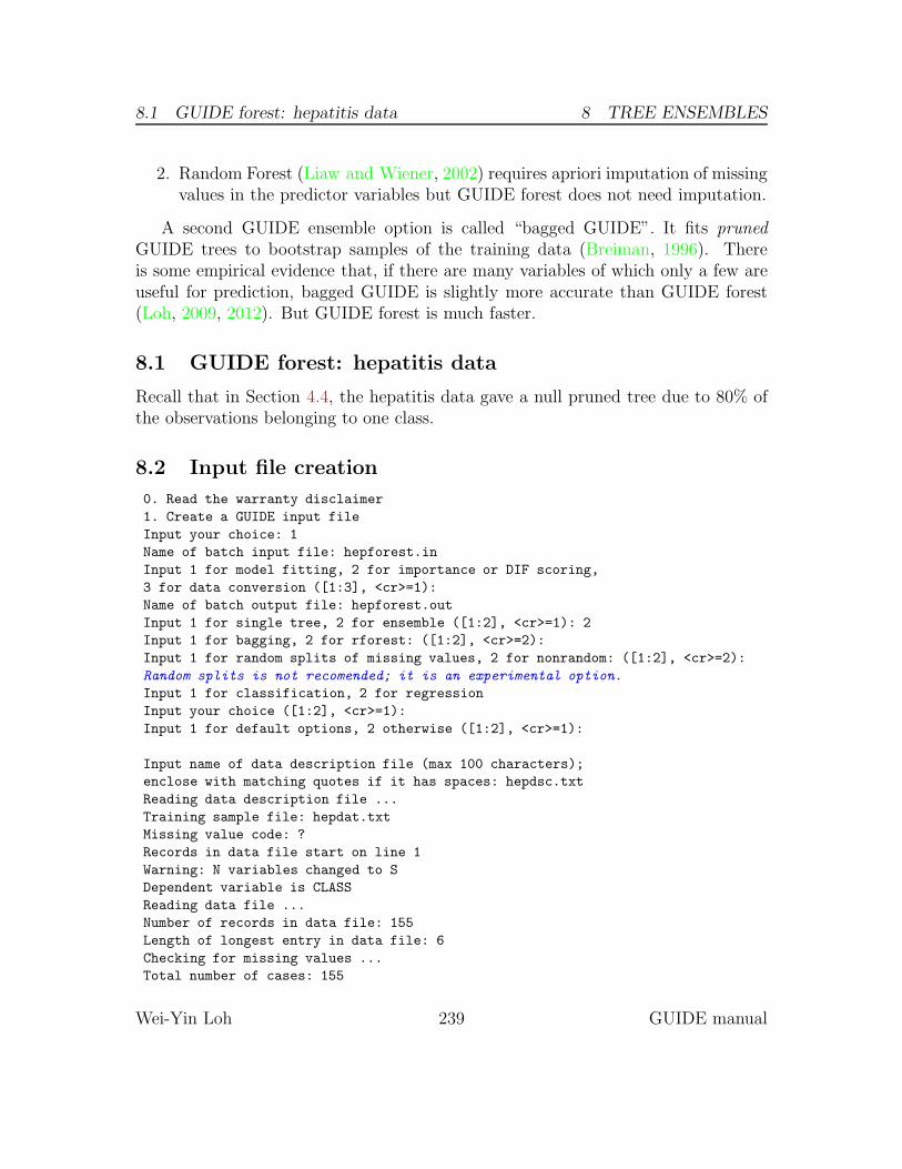
8.1 GUIDE forest: hepatitis data 8 TREE ENSEMBLES
2. Random Forest (Liaw and Wiener, 2002) requires apriori imputation of missingvalues in the predictor variables but GUIDE forest does not need imputation.
A second GUIDE ensemble option is called “bagged GUIDE”. It fits prunedGUIDE trees to bootstrap samples of the training data (Breiman, 1996). Thereis some empirical evidence that, if there are many variables of which only a few areuseful for prediction, bagged GUIDE is slightly more accurate than GUIDE forest(Loh, 2009, 2012). But GUIDE forest is much faster.
8.1 GUIDE forest: hepatitis data
Recall that in Section 4.4, the hepatitis data gave a null pruned tree due to 80% ofthe observations belonging to one class.
8.2 Input file creation
0. Read the warranty disclaimer
1. Create a GUIDE input file
Input your choice: 1
Name of batch input file: hepforest.in
Input 1 for model fitting, 2 for importance or DIF scoring,
3 for data conversion ([1:3], <cr>=1):
Name of batch output file: hepforest.out
Input 1 for single tree, 2 for ensemble ([1:2], <cr>=1): 2
Input 1 for bagging, 2 for rforest: ([1:2], <cr>=2):
Input 1 for random splits of missing values, 2 for nonrandom: ([1:2], <cr>=2):
Random splits is not recomended; it is an experimental option.
Input 1 for classification, 2 for regression
Input your choice ([1:2], <cr>=1):
Input 1 for default options, 2 otherwise ([1:2], <cr>=1):
Input name of data description file (max 100 characters);
enclose with matching quotes if it has spaces: hepdsc.txt
Reading data description file ...
Training sample file: hepdat.txt
Missing value code: ?
Records in data file start on line 1
Warning: N variables changed to S
Dependent variable is CLASS
Reading data file ...
Number of records in data file: 155
Length of longest entry in data file: 6
Checking for missing values ...
Total number of cases: 155
Wei-Yin Loh 239 GUIDE manual
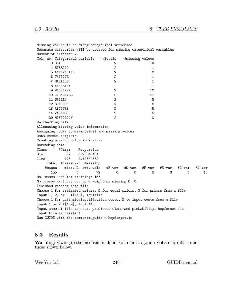
8.3 Results 8 TREE ENSEMBLES
Missing values found among categorical variables
Separate categories will be created for missing categorical variables
Number of classes: 2
Col. no. Categorical variable #levels #missing values
3 SEX 2 0
4 STEROID 2 1
5 ANTIVIRALS 2 0
6 FATIGUE 2 1
7 MALAISE 2 1
8 ANOREXIA 2 1
9 BIGLIVER 2 10
10 FIRMLIVER 2 11
11 SPLEEN 2 5
12 SPIDERS 2 5
13 ASCITES 2 5
14 VARICES 2 5
20 HISTOLOGY 2 0
Re-checking data ...
Allocating missing value information
Assigning codes to categorical and missing values
Data checks complete
Creating missing value indicators
Rereading data
Class #Cases Proportion
die 32 0.20645161
live 123 0.79354839
Total #cases w/ #missing
#cases miss. D ord. vals #X-var #N-var #F-var #S-var #B-var #C-var
155 0 72 0 0 0 6 0 13
No. cases used for training: 155
No. cases excluded due to 0 weight or missing D: 0
Finished reading data file
Choose 1 for estimated priors, 2 for equal priors, 3 for priors from a file
Input 1, 2, or 3 ([1:3], <cr>=1):
Choose 1 for unit misclassification costs, 2 to input costs from a file
Input 1 or 2 ([1:2], <cr>=1):
Input name of file to store predicted class and probability: hepforest.fit
Input file is created!
Run GUIDE with the command: guide < hepforest.in
8.3 Results
Warning: Owing to the intrinsic randomness in forests, your results may differ fromthose shown below.
Wei-Yin Loh 240 GUIDE manual
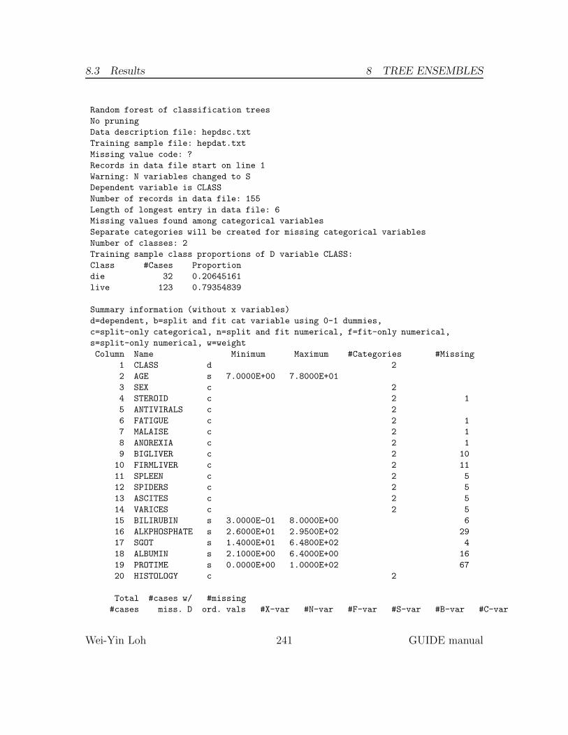
8.3 Results 8 TREE ENSEMBLES
Random forest of classification trees
No pruning
Data description file: hepdsc.txt
Training sample file: hepdat.txt
Missing value code: ?
Records in data file start on line 1
Warning: N variables changed to S
Dependent variable is CLASS
Number of records in data file: 155
Length of longest entry in data file: 6
Missing values found among categorical variables
Separate categories will be created for missing categorical variables
Number of classes: 2
Training sample class proportions of D variable CLASS:
Class #Cases Proportion
die 32 0.20645161
live 123 0.79354839
Summary information (without x variables)
d=dependent, b=split and fit cat variable using 0-1 dummies,
c=split-only categorical, n=split and fit numerical, f=fit-only numerical,
s=split-only numerical, w=weight
Column Name Minimum Maximum #Categories #Missing
1 CLASS d 2
2 AGE s 7.0000E+00 7.8000E+01
3 SEX c 2
4 STEROID c 2 1
5 ANTIVIRALS c 2
6 FATIGUE c 2 1
7 MALAISE c 2 1
8 ANOREXIA c 2 1
9 BIGLIVER c 2 10
10 FIRMLIVER c 2 11
11 SPLEEN c 2 5
12 SPIDERS c 2 5
13 ASCITES c 2 5
14 VARICES c 2 5
15 BILIRUBIN s 3.0000E-01 8.0000E+00 6
16 ALKPHOSPHATE s 2.6000E+01 2.9500E+02 29
17 SGOT s 1.4000E+01 6.4800E+02 4
18 ALBUMIN s 2.1000E+00 6.4000E+00 16
19 PROTIME s 0.0000E+00 1.0000E+02 67
20 HISTOLOGY c 2
Total #cases w/ #missing
#cases miss. D ord. vals #X-var #N-var #F-var #S-var #B-var #C-var
Wei-Yin Loh 241 GUIDE manual

8.3 Results 8 TREE ENSEMBLES
155 0 72 0 0 0 6 0 13
No. cases used for training: 155
No. cases excluded due to 0 weight or missing D: 0
Univariate split highest priority
No interaction and linear splits
Number of trees in ensemble: 500
Number of variables used for splitting: 7
Simple node models
Estimated priors
Unit misclassification costs
Fraction of cases used for splitting each node: 0.64516
Max. number of split levels: 10
Min. node sample size: 5
Mean number of terminal nodes: 10.51
Classification matrix for training sample:
Predicted True class
class die live
die 15 8
live 17 115
Total 32 123
Number of cases used for tree construction: 155
Number misclassified: 25
Resubstitution est. of mean misclassification cost: 0.1613
Predicted class probabilities are stored in hepforest.fit
Except for the number of observations misclassified, the above results are notparticularly useful; they mostly provide a record of the parameter values chosen toconstruct the forest. The predicted class probabilities in the file hepforest.fit aremore useful, the top few lines of which are shown below. The first column indicateswhether or not the observation is used for training (labeled “y” vs. “n”), followedby its predicted class probabilities. The last two columns give the predicted andobserved class labels. For example, observation 7 below has predicted proabilities of0.29997 and 0.70003 for being in class die and live, respectively, and its predictedclass is live.
train "die" "live" predicted observed
y 0.12997E-01 0.98700E+00 "live" "live"
y 0.56235E-01 0.94376E+00 "live" "live"
y 0.30716E-01 0.96928E+00 "live" "live"
y 0.83529E-02 0.99165E+00 "live" "live"
y 0.14475E-01 0.98553E+00 "live" "live"
y 0.14038E-01 0.98596E+00 "live" "live"
Wei-Yin Loh 242 GUIDE manual

8.4 Bagged GUIDE 8 TREE ENSEMBLES
y 0.29997E+00 0.70003E+00 "live" "die"
8.4 Bagged GUIDE
We now apply bagged GUIDE to the same data.
0. Read the warranty disclaimer
1. Create a GUIDE input file
Input your choice: 1
Name of batch input file: hepbag.in
Input 1 for model fitting, 2 for importance or DIF scoring,
3 for data conversion ([1:3], <cr>=1):
Name of batch output file: hepbag.out
Input 1 for single tree, 2 for ensemble ([1:2], <cr>=1): 2
Input 1 for bagging, 2 for rforest: ([1:2], <cr>=2): 1
Input 1 for classification, 2 for regression
Input your choice ([1:2], <cr>=1):
Input 1 for default options, 2 otherwise ([1:2], <cr>=1):
Input name of data description file (max 100 characters);
enclose with matching quotes if it has spaces: hepdsc.txt
Reading data description file ...
Training sample file: hepdat.txt
Missing value code: ?
Records in data file start on line 1
Warning: N variables changed to S
Dependent variable is CLASS
Reading data file ...
Number of records in data file: 155
Length of longest entry in data file: 6
Checking for missing values ...
Total number of cases: 155
Missing values found among categorical variables
Separate categories will be created for missing categorical variables
Number of classes: 2
Col. no. Categorical variable #levels #missing values
3 SEX 2 0
4 STEROID 2 1
5 ANTIVIRALS 2 0
6 FATIGUE 2 1
7 MALAISE 2 1
8 ANOREXIA 2 1
9 BIGLIVER 2 10
10 FIRMLIVER 2 11
11 SPLEEN 2 5
Wei-Yin Loh 243 GUIDE manual

8.4 Bagged GUIDE 8 TREE ENSEMBLES
12 SPIDERS 2 5
13 ASCITES 2 5
14 VARICES 2 5
20 HISTOLOGY 2 0
Re-checking data ...
Allocating missing value information
Assigning codes to categorical and missing values
Data checks complete
Creating missing value indicators
Rereading data
Class #Cases Proportion
die 32 0.20645161
live 123 0.79354839
Total #cases w/ #missing
#cases miss. D ord. vals #X-var #N-var #F-var #S-var #B-var #C-var
155 0 72 0 0 0 6 0 13
No. cases used for training: 155
No. cases excluded due to 0 weight or missing D: 0
Finished reading data file
Choose 1 for estimated priors, 2 for equal priors, 3 for priors from a file
Input 1, 2, or 3 ([1:3], <cr>=1):
Choose 1 for unit misclassification costs, 2 to input costs from a file
Input 1 or 2 ([1:2], <cr>=1):
Input name of file to store predicted class and probability: hepbag.fit
Input file is created!
Run GUIDE with the command: guide < hepbag.in
Results
Ensemble of bagged classification trees
Pruning by cross-validation
Data description file: hepdsc.txt
Training sample file: hepdat.txt
Missing value code: ?
Records in data file start on line 1
Warning: N variables changed to S
Dependent variable is CLASS
Number of records in data file: 155
Length of longest entry in data file: 6
Missing values found among categorical variables
Separate categories will be created for missing categorical variables
Number of classes: 2
Training sample class proportions of D variable CLASS:
Class #Cases Proportion
die 32 0.20645161
Wei-Yin Loh 244 GUIDE manual

8.4 Bagged GUIDE 8 TREE ENSEMBLES
live 123 0.79354839
Summary information (without x variables)
d=dependent, b=split and fit cat variable using 0-1 dummies,
c=split-only categorical, n=split and fit numerical, f=fit-only numerical,
s=split-only numerical, w=weight
Column Name Minimum Maximum #Categories #Missing
1 CLASS d 2
2 AGE s 7.0000E+00 7.8000E+01
3 SEX c 2
4 STEROID c 2 1
5 ANTIVIRALS c 2
6 FATIGUE c 2 1
7 MALAISE c 2 1
8 ANOREXIA c 2 1
9 BIGLIVER c 2 10
10 FIRMLIVER c 2 11
11 SPLEEN c 2 5
12 SPIDERS c 2 5
13 ASCITES c 2 5
14 VARICES c 2 5
15 BILIRUBIN s 3.0000E-01 8.0000E+00 6
16 ALKPHOSPHATE s 2.6000E+01 2.9500E+02 29
17 SGOT s 1.4000E+01 6.4800E+02 4
18 ALBUMIN s 2.1000E+00 6.4000E+00 16
19 PROTIME s 0.0000E+00 1.0000E+02 67
20 HISTOLOGY c 2
Total #cases w/ #missing
#cases miss. D ord. vals #X-var #N-var #F-var #S-var #B-var #C-var
155 0 72 0 0 0 6 0 13
No. cases used for training: 155
No. cases excluded due to 0 weight or missing D: 0
Univariate split highest priority
Interaction splits 2nd priority; no linear splits
Number of trees in ensemble: 100
Pruning by v-fold cross-validation, with v = 5
Selected tree is based on mean of CV estimates
Simple node models
Estimated priors
Unit misclassification costs
Fraction of cases used for splitting each node: 0.64516
Max. number of split levels: 7
Min. node sample size: 10
Number of SE’s for pruned tree: 5.0000E-01
Wei-Yin Loh 245 GUIDE manual

9 OTHER FEATURES
Mean number of terminal nodes: 1.790
Classification matrix for training sample:
Predicted True class
class die live
die 0 0
live 32 123
Total 32 123
Number of cases used for tree construction: 155
Number misclassified: 32
Resubstitution est. of mean misclassification cost: 0.2065
Predicted class probabilities are stored in hepbag.fit
The top few lines of hepbag.fit follow.
train "die" "live" predicted observed
y 0.15576E+00 0.84424E+00 "live" "live"
y 0.18353E+00 0.81647E+00 "live" "live"
y 0.15566E+00 0.84434E+00 "live" "live"
y 0.17501E+00 0.82499E+00 "live" "live"
y 0.16002E+00 0.83998E+00 "live" "live"
y 0.15634E+00 0.84366E+00 "live" "live"
y 0.19084E+00 0.80916E+00 "live" "die"
9 Other features
9.1 Pruning with test samples
GUIDE typically has three pruning options for deciding the size of the final tree:(i) cross-validation, (ii) test sample, and (iii) no pruning. Test-sample pruning isavailable only when there are no derived variables, such as creation of dummy indi-cator variables when ‘b’ variables are present. If test-sample pruning is chosen, theprogram will ask for the name of the file containing the test samples. This file musthave the same column format as the training sample file. Pruning with test-samplesor no pruning are non-default options.
Wei-Yin Loh 246 GUIDE manual

9.2 Prediction of test samples 9 OTHER FEATURES
9.2 Prediction of test samples
GUIDE can produce R code to predict future observations from all except kerneland nearest neighbor classification and ensemble models. This is also a non-defaultoption.
Predictions of the training data for all models can be obtained, however, at thetime of tree construction. This feature can be used to obtain predictions on “testsamples” (i.e., observations that are not used in tree construction) by adding themto the training sample file. There are two ways to distinguish the test observationsfrom the training observations:
1. Use a weight variable (designated as W in the description file) that takes value1 for each training observation and 0 or each test observation.
2. Replace the D values of the test observations with the missing value code.
For tree construction, GUIDE does not use observations in the training sample filethat have zero weight.
9.3 GUIDE in R and in simulations
GUIDE can be used in simulations or used repeatedly on bootstrap samples to pro-duce an ensemble of tree models. For the latter,
1. Create a file (with name data.txt, say) containing one set of bootstrappeddata.
2. Create a data description file (with name desc.txt, say) that refers to data.txt.
3. Create an input file (with name input.txt, say) that refers to desc.txt.
4. Write a batch program (Windows) or a shell script (Linux or Macintosh) thatrepeatedly:
(a) replaces the file data.txt with new bootstrapped samples;
(b) calls GUIDE with the command: guide < input.txt; and
(c) reads and processes the results from each GUIDE run.
In R, the command in step 4b depends on the operating system. If the GUIDEprogram and the files data.txt and input.txt are in the same folder as theworking R directory, the command is:
Wei-Yin Loh 247 GUIDE manual

9.4 Generation of powers and products 9 OTHER FEATURES
Linux/Macintosh: system("guide < input.txt > log.txt")
Windows: shell("guide < input.txt > log.txt")
If the files are not all in the same folder, full path names must be given. Herelog.txt is a text file that stores messages during execution. If GUIDE doesnot run successfully, errors are also written to log.txt.
9.4 Generation of powers and products
GUIDE allows the creation of certain powers and products of regressor variables onthe fly. Specifically, variables of the form Xp
1Xq2 , where X1 and X2 are numerical
predictor variables and p and q are integers, can be created by adding one or morelines of the form
0 i p j q a
at the end of the data description file. Here i and j are integers giving the columnnumbers of variables X1 and X2, respectively, in the data file and a is one of theletters n, s, or f (corresponding to a numerical variable used for both splitting andfitting, splitting only, or fitting only).
To demonstrate, suppose we wish to fit a piecewise quadratic model in the vari-able wtgain in the birthweight data. This is easily done by adding one line to thefile birthwt.dsc. First we assign the s (for splitting only) designator to every nu-merical predictor except wtgain. This will prevent all variables other than wtgain
from acting as regressors in the piecewise quadratic models. To create the variablewtgain2, add the line
0 8 2 8 0 f
to the end of birthwt.dsc. The 8’s in the above line refer to the column number ofthe variables wtgain in the data file, and the f tells the program to use the variablewtgain2 for fitting terminal node models only. Note: The line defines wtgain2 aswtgain2 × wtgain0. Since we can equivalently define the variable by wtgain2 =wtgain1 × wtgain1, we could also have used the line: “0 8 1 8 1 f”.
The resulting description file now looks like this:
birthwt.dat
NA
1
1 weight d
2 black c
Wei-Yin Loh 248 GUIDE manual

9.5 Data formatting functions 9 OTHER FEATURES
3 married c
4 boy c
5 age s
6 smoke c
7 cigsper s
8 wtgain n
9 visit c
10 ed c
11 lowbwt x
0 8 2 8 0 f
When the program is given this description file, the output will show the regressioncoefficients of wtgain and wtgain2 in each terminal node of the tree.
9.5 Data formatting functions
The program includes a utility function for reformatting data files into forms requiredby some statistical software packages:
1. R/Splus: Fields are space delimited. Missing values are coded as NA. Eachrecord is written on one line. Variable names are given on the first line.
2. SAS: Fields are space delimited. Missing values are coded with periods. Char-acter strings are truncated to eight characters. Spaces within character stringsare replaced with underscores (_).
3. TEXT: Fields are comma delimited. Empty fields denote missing values. Char-acter strings longer than eight characters are truncated. Each record is writtenon one line. Variable names are given on the first line.
4. STATISTICA: Fields are comma delimited. Commas in character strings arestripped. Empty fields denote missing values. Each record occupies one line.
5. SYSTAT: Fields are comma delimited. Strings are truncated to eight char-acters. Missing character values are replaced with spaces, missing numericalvalues with periods. Each record occupies one line.
6. BMDP: Fields are space delimited. Categorical values are sorted in alphabeticorder and then assigned integer codes. Missing values are indicated by asterisks.Variable names longer than eight characters are truncated.
Wei-Yin Loh 249 GUIDE manual

9.5 Data formatting functions 9 OTHER FEATURES
7. DataDesk: Fields are space delimited. Missing categorical values are codedwith question marks. Missing numerical values are coded with asterisks. Eachrecord is written on one line. Spaces within categorical values are replaced withunderscores. Variable names are given on the first line of the file.
8. MINITAB: Fields are space delimited. Categorical values are sorted in alpha-betic order and then assigned integer codes. Missing values are coded withasterisks. Variable names longer than eight characters are truncated.
9. NUMBERS: Same as TEXT option except that categorical values are con-verted to integer codes.
10. C4.5: This is the format required by the C4.5 (Quinlan, 1993) program.
11. ARFF: This is the format required by the WEKA (Witten and Frank, 2000)programs.
Following is a sample session where the hepatitis data are reformatted for R orSplus.
0. Read the warranty disclaimer
1. Create an input file for model fitting or importance scoring (recommended)
2. Convert data to other formats without creating input file
Input your choice: 3
Input name of log file: log.txt
Input 1 if D variable is categorical, 2 if real ([1:2], <cr>=1):
Input name of data description file (max 100 characters);
enclose with matching quotes if it has spaces: hepdsc.txt
Reading data description file ...
Training sample file: hepdat.txt
Missing value code: ?
Records in data file start on line 1
Warning: N variables changed to S
Dependent variable is CLASS
Reading data file ...
Number of records in data file: 155
Length of longest data entry: 6
Checking for missing values ...
Total number of cases: 155
Number of classes = 2
Col. no. Categorical variable #levels #missing values
3 SEX 2 0
4 STEROID 2 1
Wei-Yin Loh 250 GUIDE manual

REFERENCES REFERENCES
5 ANTIVIRALS 2 0
6 FATIGUE 2 1
7 MALAISE 2 1
8 ANOREXIA 2 1
9 BIGLIVER 2 10
10 FIRMLIVER 2 11
11 SPLEEN 2 5
12 SPIDERS 2 5
13 ASCITES 2 5
14 VARICES 2 5
20 HISTOLOGY 2 0
Choose one of the following data formats:
Field Miss.val.codes
No. Name Separ char. numer. Remarks
------------------------------------------------------------------
1 R/Splus space NA NA 1 line/case, var names on 1st line
2 SAS space . . strings trunc., spaces -> ’_’
3 TEXT comma empty empty 1 line/case, var names on 1st line
4 STATISTICA comma empty empty 1 line/case, commas stripped
var names on 1st line
5 SYSTAT comma space . 1 line/case, var names on 1st line
strings trunc. to 8 chars
6 BMDP space * strings trunc. to 8 chars
cat values -> integers (alph. order)
7 DATADESK space ? * 1 line/case, var names on 1st line
spaces -> ’_’
8 MINITAB space * cat values -> integers (alph. order)
var names trunc. to 8 chars
9 NUMBERS comma NA NA 1 line/case, var names on 1st line
cat values -> integers (alph. order)
10 C4.5 comma ? ? 1 line/case, dependent variable last
11 ARFF comma ? ? 1 line/case
------------------------------------------------------------------
0 abort this job
Input your choice ([0:11], <cr>=1):
Input name of new data file: hep.rdata
Follow the commented lines in "hep.rdata" to read the data into R or Splus
References
Breiman, L. (1996). Bagging predictors. Machine Learning, 24:123–140.
Breiman, L. (2001). Random forests. Machine Learning, 45:5–32.
Wei-Yin Loh 251 GUIDE manual

REFERENCES REFERENCES
Breiman, L., Friedman, J. H., Olshen, R. A., and Stone, C. J. (1984). Classificationand Regression Trees. Wadsworth, Belmont.
Broekman, B. F. P., Niti, M., Nyunt, M. S. Z., Ko, S. M., Kumar, R., and Ng,T. P. (2011). Validation of a brief seven-item response bias-free GeriatricDepression Scale. American Journal of Geriatric Psychiatry, 19:589–596.
Broekman, B. F. P., Nyunt, S. Z., Niti, M., Jin, A. Z., Ko, S. M., Kumar, R.,Fones, C. S. L., and Ng, T. P. (2008). Differential item functioning of theGeriatic Depression Scale in an Asian population. Journal of Affective Disorders,108:285–290.
Chan, K.-Y. and Loh, W.-Y. (2004). LOTUS: An algorithm for building accurateand comprehensible logistic regression trees. Journal of Computational andGraphical Statistics, 13:826–852.www.stat.wisc.edu/~loh/treeprogs/lotus/lotus.pdf.
Chaudhuri, P., Huang, M.-C., Loh, W.-Y., and Yao, R. (1994).Piecewise-polynomial regression trees. Statistica Sinica, 4:143–167.www3.stat.sinica.edu.tw/statistica/j4n1/j4n18/j4n18.htm.
Chaudhuri, P., Lo, W.-D., Loh, W.-Y., and Yang, C.-C. (1995). Generalizedregression trees. Statistica Sinica, 5:641–666.www3.stat.sinica.edu.tw/statistica/j5n2/j5n217/j5n217.htm.
Chaudhuri, P. and Loh, W.-Y. (2002). Nonparametric estimation of conditionalquantiles using quantile regression trees. Bernoulli, 8:561–576.www.stat.wisc.edu/~loh/treeprogs/guide/quantile.pdf.
Choi, Y., Ahn, H., and Chen, J. J. (2005). Regression trees for analysis of countdata with extra poisson variation. Computational Statistics & Data Analysis,49(3):893–915.
Hosmer, D. W., Lemeshow, S., and May, S. (2008). Applied Survival Analysis.Wiley, 2nd edition.
Hothorn, T. (2017). TH.data: TH’s Data Archive. R package version 1.0-8.
Ilter, N. and Guvenir, H. A. (1998). UCI machine learning repository.
Italiano, A. (2011). Prognostic or predictive? It’s time to get back to definitions!Journal of Clinical Oncology, 29:4718.
Wei-Yin Loh 252 GUIDE manual

REFERENCES REFERENCES
Kim, H. and Loh, W.-Y. (2001). Classification trees with unbiased multiway splits.Journal of the American Statistical Association, 96:589–604.www.stat.wisc.edu/~loh/treeprogs/cruise/cruise.pdf.
Kim, H. and Loh, W.-Y. (2003). Classification trees with bivariate lineardiscriminant node models. Journal of Computational and Graphical Statistics,12:512–530. www.stat.wisc.edu/~loh/treeprogs/cruise/jcgs.pdf.
Kim, H., Loh, W.-Y., Shih, Y.-S., and Chaudhuri, P. (2007). Visualizable andinterpretable regression models with good prediction power. IIE Transactions,39:565–579. www.stat.wisc.edu/~loh/treeprogs/guide/iie.pdf.
Koenker, R. (2005). Quantile Regression. Cambridge University Press.
Koenker, R. W. and Bassett, G. (1978). Regression quantiles. Econometrica,46:33–50.
Koenker, R. W. and Hallock, K. (2001). Quantile regression: an introduction.Journal of Economic Perspectives, 15:143–156.
Liaw, A. and Wiener, M. (2002). Classification and regression by randomforest. RNews, 2(3):18–22.
Loh, W.-Y. (2002). Regression trees with unbiased variable selection andinteraction detection. Statistica Sinica, 12:361–386.www3.stat.sinica.edu.tw/statistica/j12n2/j12n21/j12n21.htm.
Loh, W.-Y. (2006a). Logistic regression tree analysis. In Pham, H., editor,Handbook of Engineering Statistics, pages 537–549. Springer.www.stat.wisc.edu/~loh/treeprogs/lotus/springer.pdf.
Loh, W.-Y. (2006b). Regression tree models for designed experiments. In Rojo, J.,editor, The Second Erich L. Lehmann Symposium–Optimality, volume 49, pages210–228. Institute of Mathematical Statistics Lecture Notes-Monograph Series.arxiv.org/abs/math.ST/0611192.
Loh, W.-Y. (2008a). Classification and regression tree methods. In Ruggeri, F.,Kenett, R., and Faltin, F. W., editors, Encyclopedia of Statistics in Quality andReliability, pages 315–323. Wiley, Chichester, UK.www.stat.wisc.edu/~loh/treeprogs/guide/eqr.pdf.
Wei-Yin Loh 253 GUIDE manual

REFERENCES REFERENCES
Loh, W.-Y. (2008b). Regression by parts: Fitting visually interpretable modelswith GUIDE. In Chen, C., Hardle, W., and Unwin, A., editors, Handbook ofComputational Statistics, pages 447–469. Springer.www.stat.wisc.edu/~loh/treeprogs/guide/handbk.pdf.
Loh, W.-Y. (2009). Improving the precision of classification trees. Annals ofApplied Statistics, 3:1710–1737.www.stat.wisc.edu/~loh/treeprogs/guide/aoas260.pdf.
Loh, W.-Y. (2011). Classification and regression trees. Wiley InterdisciplinaryReviews: Data Mining and Knowledge Discovery, 1:14–23.http://www.stat.wisc.edu/~loh/treeprogs/guide/wires11.pdf.
Loh, W.-Y. (2012). Variable selection for classification and regression in large p,small n problems. In Barbour, A., Chan, H. P., and Siegmund, D., editors,Probability Approximations and Beyond, volume 205 of Lecture Notes inStatistics—Proceedings, pages 133–157, New York. Springer.www.stat.wisc.edu/~loh/treeprogs/guide/lchen.pdf.
Loh, W.-Y. (2014). Fifty years of classification and regression trees (withdiscussion). International Statistical Review, 34:329–370.http://www.stat.wisc.edu/~loh/treeprogs/guide/LohISI14.pdf.
Loh, W.-Y., Chen, C.-W., and Zheng, W. (2007). Extrapolation errors in linearmodel trees. ACM Trans. Knowl. Discov. Data, 1(2):6.www.stat.wisc.edu/~loh/treeprogs/guide/acm.pdf.
Loh, W.-Y., Fu, H., Man, M., Champion, V., and Yu, M. (2016). Identification ofsubgroups with differential treatment effects for longitudinal and multiresponsevariables. Statistics in Medicine, 35:4837–4855.www.stat.wisc.edu/~loh/treeprogs/guide/LFMCY16.pdf.
Loh, W.-Y., He, X., and Man, M. (2015). A regression tree approach to identifyingsubgroups with differential treatment effects. Statistics in Medicine,34:1818–1833. www.stat.wisc.edu/~loh/treeprogs/guide/LohHeMan15.pdf.
Loh, W.-Y. and Shih, Y.-S. (1997). Split selection methods for classification trees.Statistica Sinica, 7:815–840.www3.stat.sinica.edu.tw/statistica/j7n4/j7n41/j7n41.htm.
Wei-Yin Loh 254 GUIDE manual

REFERENCES REFERENCES
Loh, W.-Y. and Vanichsetakul, N. (1988). Tree-structured classification viageneralized discriminant analysis (with discussion). Journal of the AmericanStatistical Association, 83:715–728.www.stat.wisc.edu/~loh/treeprogs/fact/LV88.pdf.
Loh, W.-Y. and Zheng, W. (2013). Regression trees for longitudinal andmultiresponse data. Annals of Applied Statistics, 7:495–522.www.stat.wisc.edu/~loh//treeprogs/guide/AOAS596.pdf.
Marc, L. G., Raue, P. J., and Bruce, M. L. (2008). Screening performance of the15-item Geriatric Depression Scale in a diverse elderly home care population.American Journal of Geriatric Psychiatry, 16:914–921.
Murnane, R. J., Boudett, K. P., and Willett, J. B. (1999). Do male dropoutsbenefit from obtaining a GED, postsecondary education, and training?Evaluation Reviews, 23:475–502.
Peters, A. and Hothorn, T. (2015). ipred: Improved Predictors. R package version0.9-5.
Quinlan, J. R. (1992). Learning with continuous classes. In 5th Australian JointConference on Artificial Intelligence, pages 343–348.
Quinlan, J. R. (1993). C4.5: Programs for Machine Learning. Morgan Kaufmann.
Rousseeuw, P. J. and Leroy, A. M. (1987). Robust Regression and OutlierDetection. Wiley.
Schmoor, C., Olschewski, M., and Schumacher, M. (1996). Randomized andnon-randomized patients in clinical trials: experiences with comprehensive cohortstudies. Statistics in Medicine, 15:263–271.
Segal, M. R. (1988). Regression trees for censored data. Biometrics, 44:35–47.
Singer, J. D. and Willett, J. B. (2003). Applied Longitudinal Data Analysis. OxfordUniversity Press, New York, NY.
Therneau, T., Atkinson, B., and Ripley, B. (2017). rpart: Recursive Partitioningand Regression Trees. CRAN.R-project.org/package=rpart.
Witten, I. and Frank, E. (2000). Data Mining: Practical Machine Learning Toolsand Techniques with JAVA Implementations. Morgan Kaufmann, San Fransico,CA. www.cs.waikato.ac.nz/ml/weka.
Wei-Yin Loh 255 GUIDE manual


