
1
Hazard Assessment for the
Eemskanaal area
of the Groningen field
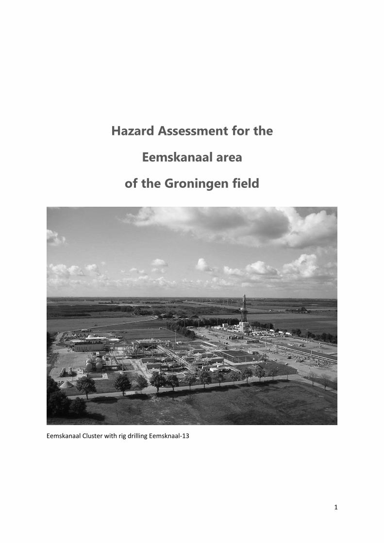
Eemskanaal Cluster with rig drilling Eemsknaal-13

2
Contents Hazard Assessment for the ..................................................................................................................... 1
Eemskanaal area ..................................................................................................................................... 1
of the Groningen field ............................................................................................................................. 1
Introduction ........................................................................................................................................ 3
The Eemskanaal Cluster of the Groningen Field ................................................................................. 4
Subsidence observations in the Eemskanaal Area.............................................................................. 5
Groningen Field Model ..................................................................................................................... 11
General .......................................................................................................................................... 11
Improvements ............................................................................................................................... 11
Static Model .................................................................................................................................. 13
Dynamic Model ............................................................................................................................. 16
Model 1: [[Model 40]] .................................................................................................................. 18
Model 2: [[Model 38]] .................................................................................................................. 21
Conclusion ..................................................................................................................................... 23
Subsidence and compaction in the Eemskanaal ............................................................................... 24
Subsidence calibration .................................................................................................................. 26
Scenarios ........................................................................................................................................... 27
Modelling Eemskanaal .................................................................................................................. 27
Results of Compaction modelling ................................................................................................. 29
Compaction differences ................................................................................................................ 31
Seismic Response and Hazard ........................................................................................................... 34
Methodology ................................................................................................................................. 34
Probabilistic Seismic Hazard Assessments .................................................................................... 35
Reference Model ........................................................................................................................... 35
Base Case Model ........................................................................................................................... 38
Compaction Model Sensitivity ...................................................................................................... 42
Production Sensitivity ................................................................................................................... 44
Sub-surface Model Uncertainty .................................................................................................... 47
Conclusions ....................................................................................................................................... 49
References ........................................................................................................................................ 50
Appendix A History Match Groningen Model .............................................................................. 51
Appendix B Hazard Maps for the Eemskanaal Area of the Groningen field ................................ 52

3
Introduction After an earthquake of magnitude 2.8 on September 30, 2014 in Ten Boer and the subsequent
parliamentary debate, the minister of Economic Affairs requested a renewed assessment of the
earthquake hazard for the Groningen gas field with a specific focus on the Eemskanaal area around
the Eemskanaal production cluster. A review of this area of the field is pertinent because of its
relative proximity to the city of Groningen and its unique technical nature, making it more difficult to
assess the seismic hazard.
Based on the latest production figures and forecasts and several model improvements a set of
seismic hazard maps were generated in order to assess whether there is a significant increase in
induced seismic hazard near the city of Groningen.

4
The Eemskanaal Cluster of the Groningen Field Groningen production cluster Eemskanaal is a king-size cluster producing from 13 wells. It is located
in the south-western part of the Groningen field. Twelve of these wells produce from the
Eemskanaal area directly below the cluster. Eemskanaal-13 is a deviated well producing from the
Harkstede block located south-west of the Eemskanaal cluster.
Gas from the cluster is produced into the Groningen production ring pipeline. Via the nearby located
custody transfer-station Overslag Eemskanaal, the gas is evacuated to the Gas Transport Services
(GTS) grid.
The gas produced from the Eemskanaal cluster has a different composition and calorific value
compared to the gas from the other Groningen clusters. It has a Wobbe Index of average 45.7,
compared to a value of 43.7 for the other Groningen clusters. Groningen gas can only be delivered
when its composition is within the narrow Groningen Gas Quality band. The maximum contractual
Wobbe value is 44.2. Currently, the Eemskanaal gas can only be produced when it is mixed with a
sufficiently large volume of gas from other Groningen clusters.
The Eemskanaal gas is mixed in the ring pipeline with gas produced by other Groningen clusters to
meet the gas delivery quality specifications. Consequently, the contribution of the Eemskanaal
cluster to the overall Groningen field production strongly depends on the off-take of sales gas on
Overslag Eemskanaal by GTS. In periods of low demand, less gas is available for mixing with gas
produced from the Eemskanaal cluster.
Currently, the technically maximum Eemskanaal capacity is estimated at 17 million Nm3/d without
the quality constraint. Under current operating conditions for the field offtake, the production is
estimated to be, approximately 8 million Nm3 per day on a monthly averaged basis.
Figure 1 Areal overview of the Eemskanaal Cluster

5
Subsidence observations in the Eemskanaal Area Gas production from the Groningen field leads to subsidence at the surface. Subsidence in the
Groningen field area is monitored since 1964 through levelling surveys, and since 1992 also through
satellite observation. The monitoring capacity was further extended in March 2013 with the
installation of two GPS stations at the Ten Post and Veendam production locations. Ten additional
GPS stations were installed early 2014 (Figure 2).
Figure 2 Location of the 11 GPS stations for subsidence monitoring in the field.
One of the new GPS stations was placed on the Eemskanaal cluster. Data obtained from this station
indicate a subsidence of some 5 mm at this location for the period from 20 February to 28
September 2014, (Figure 3 and 4) .

6
Figure 3 Results from the permanent subsidence monitoring GPS station at the Eemskanaal
Cluster.
Figure 4 Estimated subsidence at the Eemskanaal Cluster location since the installation of the
GPS station in February 2014. Production from the Eemskanaal Cluster is also shown.

7
The levelling surveys meet the specifications for monitoring of NAP set by Rijkswaterstaat. These
specifications have been prescribed in ‘Productspecificaties Beheer NAP, Secundaire waterpassingen
t.b.v. de bijhouding van het NAP, versie 1.1 van januari 2008’.
The results of the levelling surveys are made available to SodM in the form of a state of difference
(differentiestaat). This includes the levelling data obtain by or commissioned by Rijkswaterstaat. The
state of differences is based on estimated heights, using a free network adjustment, for each epoch.
Identification errors in the historical measurements have not been removed. This means outliers
can occur in this data. Furthermore, no distinction has been made between autonomous movement
of the levelling benchmarks and movement as a result of gas production.
The movement of a levelling benchmark located in the Eemskanaal Area is shown in figure 5.
Figure 5 Example: Levelling benchmark 007G0180 located south of the Eemskanaal Cluster
location shows good correspondence between the subsidence measured by levelling
surveys [white squares with uncertainty indication] and satellite measurements [green
circle markers indicate one-year averages].
An overview of subsidence measured in the Eemskanaal area in the period 2007 to 2012 is shown in
figure 6. This shows good correspondence between levelling survey results and satellite (InSAR)
measurements.

8
Figure 6 Subsidence measurements in the Eemskanaal Area from levelling surveys (red) and
satellite measurements (blue) over a 5-year period (2007 – 2012). Values (in mm)
represent the change in relative height that occurred over the 5-year period.
Benchmark stability can be an issue. This is illustrated by the two example benchmarks discussed
below.
Figure 7a Levelling benchmark 007G0139 north-east of the Eemskanaal cluster shows high
subsidence while surrounding benchmarks show subsidence in line with the regional
trend. Also in the period 2003 to 2008 this benchmark showed large height reduction of
-14.867
-14.899 -14.921
-14.957
-15.034
-15.138
-15.20
-15.15
-15.10
-15.05
-15.00
-14.95
-14.90
-14.85
-14.80
-14.75
-14.70
8/1
/19
87
11
/1/1
98
8
2/1
/19
90
5/1
/19
91
8/1
/19
92
11
/1/1
99
3
2/1
/19
95
5/1
/19
96
8/1
/19
97
11
/1/1
99
8
2/1
/20
00
5/1
/20
01
8/1
/20
02
11
/1/2
00
3
2/1
/20
05
5/1
/20
06
8/1
/20
07
11
/1/2
00
8
2/1
/20
10
5/1
/20
11
8/1
/20
12
Peilmerk 007G0139
�007G0139
9
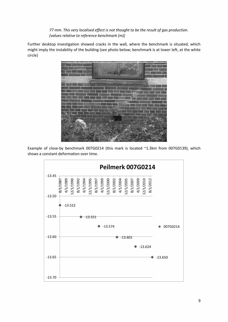
77 mm. This very localised effect is not thought to be the result of gas production.
(values relative to reference benchmark (m))
Further desktop investigation showed cracks in the wall, where the benchmark is situated, which
might imply the instability of the building (see photo below; benchmark is at lower left, at the white
circle)
Example of close-by benchmark 007G0214 (this mark is located ~1.3km from 007G0139), which
shows a constant deformation over time.
-13.522
-13.551
-13.574
-13.601
-13.624
-13.650
-13.70
-13.65
-13.60
-13.55
-13.50
-13.45
8/1
/19
87
4/1
/19
89
12
/1/1
99
0
8/1
/19
92
4/1
/19
94
12
/1/1
99
5
8/1
/19
97
4/1
/19
99
12
/1/2
00
0
8/1
/20
02
4/1
/20
04
12
/1/2
00
5
8/1
/20
07
4/1
/20
09
12
/1/2
01
0
8/1
/20
12
Peilmerk 007G0214
�007G0214
10
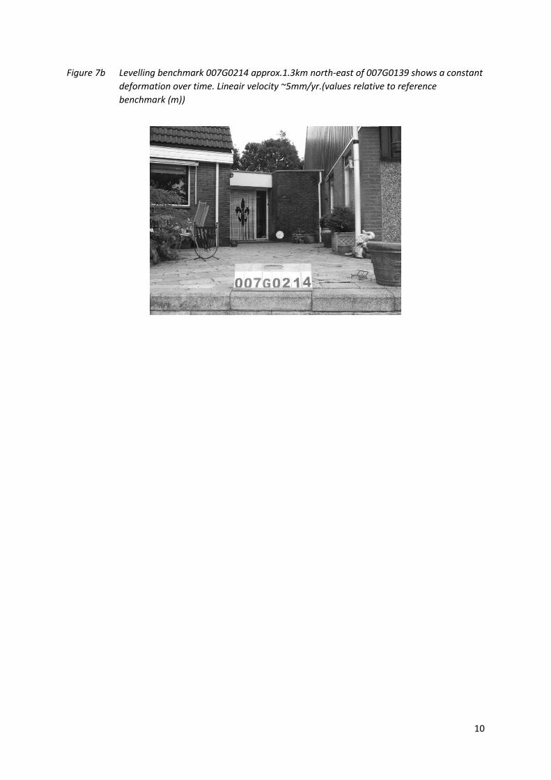
Figure 7b Levelling benchmark 007G0214 approx.1.3km north-east of 007G0139 shows a constant
deformation over time. Lineair velocity ~5mm/yr.(values relative to reference
benchmark (m))
11
Groningen Field Model
General
Calculation of seismic hazard is based on output from static and dynamic models. Results from the
Groningen Field Review (GFR2012) used for the update of the Winningsplan 2013, showed a
relatively poor match in the south-west part of the field. This section describes the improvements
made to the model to obtain a closer match between model performance and actual field
behaviour.
Improvements
The Groningen full field history match in general is of good quality. The typical pressure mismatch is
in the order of only a few bars (RMS). However, in some of the peripheral areas of the field, where
aquifers are connected to the field, discrepancies exist with respect to water encroachment into the
field. As well density is often lower in these areas, observations of pressure and water rise can be
scarce. Some of the discrepancies observed between modelled and measured subsidence can be
traced back to the uncertainty in compaction in these areas, which in turn is related to porosity and
pressure uncertainties. In the 2013 winningsplan, two different models G1 and G2 were therefore
used.
· The focus for the G1 model has been to obtain an improved compaction/subsidence match
in the Loppersum Area; and match for pressure and water encroachment in the south-west
peripheral area was compromised
· The G2 model resulted in a good reservoir pressure history match, but the subsidence match
was compromised
Attempts to build a single model to match all observations were not successful. The history match
for both the G1 and G2 models showed discrepancies in the Eemskanaal (Figure 8) and Harkstede
areas. In particular the production from the only well producing from the Harkstede block,
Eemskanaal-13, was poorly matched (Figure 9 and Figure 10).

12
Figure 8 Production from the Eemskanaal Cluster (wells EKL-1 to EKL-12, i.e. excluding EKL13)
model (G1) results compared to actual production for January to September 2014. In
September 2014 these wells did not produce because of a planned three-yearly
maintenance and inspection shutdown.
Figure 9 The production from well EKL-13 producing from the Harkstede block, comparison
between model results and actual production. Due to excessive water production in the
model, the well suffers from lift die-out and is not able to produce gas. In reality, the
well has produced gas during the first three months of 2014. The well has been closed-in
since April.

13
Figure 10 Production from EKL-13, The excessive water production from this well in the G1 model
causes the well to stop production due to lift die-out. Dots are production data and the
lines are G1 model results.
This poor match between field performance observations and modelling results is most likely related
to the uncertainties in the geological model of that peripheral part of the Groningen field. These
uncertainties are described below.
Static Model
The poor match between observations and modelling results is most likely related to the
uncertainties in the geological model of the peripheral part of the Groningen field. A better match
can probably be obtained with an increased static volume in the Harkstede block compared to base
case static model. This is a feasible option if such an increase can be realized within the uncertainties
of the dominant input parameters, i.e. bulk rock volume and porosity. These uncertainties are
evaluated in the following.
Porosity uncertainty
Maps 1 to 4 in figures 11 and 12 show the average porosity per reservoir zone in the south-west
periphery of the Groningen field. The maps are derived from up-scaled wireline log measurements
from wells in the area, which are interpolated using a convergent gridding algorithm. The average
porosity in the Harkstede block ranges from approximately 14 to 15.5%. These values are consistent
with the observed values for neighboring wells in the area. The relative uncertainty as reported in
the GFR2012 Field Review document is 0.022 (= 1 SD). This means that the maximum porosity in the
Harkstede block could be as high as 16.2% (= 15.5 + 2 SD).

14
Figure 11 Porosity [faction] for the Upper Slochteren Sandstone Formation is shown for reservoir
layers 2 and 3.
Figure 12 Porosity [faction] for the Upper Slochteren Sandstone Formation reservoir layer1 and the
Lower Slochteren Formation reservoir layers 2.
Top map uncertainty
Figure 13 shows a structural map of the Top Rotliegend horizon in the South-West periphery. The
method for establishing the uncertainty in this map is described in the same GFR2012 document,
and is presented as a 1 SD uncertainty map. Figure 14 shows this uncertainty map zoomed in for the
Map 1: USS.3res Map 2: USS.2res
KPD
KHM
EKL
HRS
TBR
BDM
FRB
Map 3: USS.1res Map 4: LSS.2res

15
Harkstede area. Uncertainties at the well locations (EKL-13, HRS-1 and HRS-2A) are (close to) zero.
Away from these well control points, the uncertainty in the block grows to a maximum of 22 m. The
average uncertainty for the whole block will be slightly over 10 m.
Figure 13 Structural map of the Top Rotliegend horizon in the SW periphery.
Map 5: Top_Rotliegend structural map of the Groningen SW Periphery
EKL
HRS
TBR

16
Figure 14 The uncertainty map zoomed in for the Harkstede area.
Based on this assessment of the uncertainties in the geological data, it was concluded that the
porosity in the Harkstede block is unlikely to be more than 1.5 % higher than in the reservoir model,
while the uncertainty in the top of the reservoir could increase away from the Eemskanaal-13 well
and the Harkstede-1 well to some 20 meters. The limit of the uncertainty in porosity was therefore
set at + 1.5% and for top reservoir top at 10 meters average for the block.
Dynamic Model Two different history matched models will be used in this Eemskanaal hazard assessment. Both
models are based on the G1 model used for the hazard assessment in the Winningsplan 2013, and
are here referred to as Models 1 (STR40) and 2 (STR38). With both models, a good match is obtained
for all wells of the Eemskanaal Cluster including EKL-13 in the Harkstede block (Figures 15 and 16).
Together, these two models capture the inherent volumetric uncertainty in the static reservoir
model.
HRS
Map 6: Depth uncertainty map for the Groningen SW Periphery

17
Figure 15 Modelled and actual production from the Eemskanaal Area (wells EKL-1 to EKL12, i.e.
excluding EKL13, improved G1 model) for the period January to September 2014. In
September 2014 these wells did not produce because of a planned three-yearly
maintenance and inspection shutdown.
Figure 16 Modelled and actual production from well EKL-13 in the Harkstede block, (improved G1
model). EKL-13 is the only well producing from the Harkstede block. The well has been
closed-in since April.

18
Model 1 [Model 40]
In Model 1, the following changes have been made to the G1 model,:
· Harkstede block structure on average 10 meters shallower,
· Porosity in the Harkstede block is increased by 1.5%,
· Permeability in the Harkstede Noord block is increased,
· Permeability in the aquifer in the South West periphery is reduced and
· The transmissibility of two faults in the South West periphery is reduced.
A complete rebuild of the structural model was not feasible within the time frame for this
evaluation. Therefore, the shallower structure was approximated by a local lowering of the GWC
with 10 m.
With these changes to the G1 model, an improved history match for the Harkstede block was
achieved. Well Eemskanaal-13 in the original G1 model stopped producing due to lift die-out. In the
new Model 1, the same well was able to produce the observed gas production volumes. A very good
match between observed and modelled reservoir pressure was obtained for all wells of the
Eemskanaal cluster. The pressure match for the two wells located in the Harkstede block is in model
1 also good (Figures 17 and 18).
Water production from the Eemskanaal-13 well in Model 1 is reduced compared to the original G1
model. The well produced about 12 m3/day formation water over the last 5 years (WGR is
approximately double that of condensed water alone) and Model 1 shows a water rate of about 3
m3/day, see Figure 19. Note that condensed water is not modelled explicitly by the models.
Figure 17 Model 1: Pressure match for the wells producing from the Eemskanaal Area (EKL-1 to
EKL-12).

19
Figure 18 Model 1: Pressure match for the two wells located in the Harkstede block. Left:
Producing well EKL-13 and Right: Observation well HRS-2A. The blue squares are high-
confidence SPTG pressure data and the pink squares are lower-confidence reservoirs
pressures calculated from closed-in THP data.
Figure 19a Model 1: Production Match for EKL-13 for Model 1. The excessive formation water
production from the G1 model has been reduced in Model 1. The connected dots are
production data and the lines are the model results. Note that the condensed water is
not explicitly modelled and that condensed water has a WGR of about 6 m3/mln m
3 at
the current field conditions.

20
Figure 19b Model 1: Water rise seen in the wells in the Harkstede block. Comparison of measured
observations (PNL logs) and model results. Left well is Eemskanaal-13, well Harkstede-
2A to the right.

21
Model 2 [Model 38]
An alternative model was prepared to further evaluate the impact of the sub-surface uncertainty.
This Model 2 is also based on the G1 model from the 2013 winningsplan. The same changes were
applied as for Model 1, with the addition that the aquifers west of the Harkstede block and
Eemskanaal area (the so-called Lauwerszee A and B aquifers) were assumed to be very poorly
connected to the gas reservoir.
Figure 20 Model 2: Pressure match for the wells producing from the Eemskanaal Area (EKL-1 to
EKL-12).
Figure 21 Model 2: Pressure match for the two wells located in the Hartstede block. Right:
Producing well EKL-13 and Right: Observation well HRK-1.

22
Figure 22 Model 2: Production Match for EKL-13. The excessive water production from the G1
model has been reduced in Model 2. The connected dots are production data and the
lines are the model results. Note that the condensed water is not explicitly modelled and
that condensed water has a WGR of about 6 m3/mln m
3 at the current field conditions.
Figure 23 Model 2: Water rise seen in the wells in the Harkstede block. Comparison of measured
observations and modelling results. Left well Harkstede-2A and Right Eemsknaal-13
In general, the performance of Model 1 is similar to Model 2. The history match quality for the two
wells in the Harkstede block is slightly poorer. Model 2 predicts a lower reservoir pressure for both
wells than actually observed for this block. The difference is in the order of 10 bar.
The reservoir pressure distribution in 2014 of the two models for the Eemskanaal area is shown in
figure 24.

23
Figure 24 Pressure map of upper Slochteren reservoir for Oct 2014. Left: model 1 with the
Lauwerszee A&B aquifers on the western edge (higher pressures) and Right: model 2
Conclusion The Groningen reservoir model G1 was updated with an improved match (historical) to better
predict (future) production and pressures in the Harkstede area and EKL cluster area. This resulted in
two different reservoir scenarios; Model 1 [40] with the same Lauwerszee aquifers as for the G1
model and model 2 [38] with a very poor connection to the Lauwerszee aquifers on the South-
Western edge of the model. Both models result in an acceptable match to the historical reservoir
pressures and gas production. In this note the effects of these changes on the geomechanical
modelling are discussed.

24
Subsidence and compaction in the Eemskanaal The results of the improved history matched models as described in the previous section have been
used to make new compaction and subsidence calculations. These were carried out with both the
Time-decay and the RTCiM compaction models. As the reservoir pressure updates are relatively
minor, the geomechanical parameters used for the Time-decay compaction model were copied from
the model used in the Winningsplan (2013). The RTCiM parameters were taken from the TNO report
(Ref. 3).
The main parameters used in the Time-decay compaction model are:
Cm factor: 0.45
Decay time: 7.3 year
For the RTCiM compaction model:
Cm factor α = 0.57 [-]
Cm,a/Cm,ref = 0.44 [-]
b = 0.017 [-]
The goodness of fit is checked by means of an RMS calculation. The RMS is defined as
Subsidence measurements were used as reported in the state of differences 000A2080_1964-01-
01_NN2013.csv, which is the “Concept State of differences ” (differentie staat) reported to SodM
(van Lieshout dd 29 Oct 2014).
For this calculation all stable benchmarks, as defined in the state of differences , were used. The
RMS was calculated using each benchmark and each epoch starting with the first measurement of
this benchmark.

25
The epochs used in the RMS calculations are
H_15_04_1964 D_10_12_1994 D_10_12_2005
H_01_09_1972 D_11_12_1995 D_10_12_2006
H_01_09_1975 D_10_12_1996 D_11_12_2007
H_15_07_1978 H_13_06_1997 H_13_08_2008
H_01_07_1981 D_10_12_1997 D_10_12_2008
H_01_09_1985 H_05_06_1998 D_10_12_2009
H_01_08_1987 D_10_12_1998 D_10_12_2010
H_15_05_1990 D_11_12_1999 D_11_12_2011
H_14_05_1991 D_10_12_2000 D_10_12_2012
D_10_12_1992 H_17_06_2003 H_25_04_2013
H_28_06_1993 D_11_12_2003
D_10_12_1993 D_10_12_2004
Table 1 Epochs available in the state of differences
An epoch name starting with an H indicates a leveling survey and a period starting with a D indicates
an InSAR survey.
The benchmarks used in the RMS calculation are selected from the South-West area of the
Groningen field, i.e. the area of the Eemskanaal cluster (Figure 24) (see section Subsidence
Observations).
Figure 24 Area of interest (purple polygon). The gray line indicates the EKL-13 well trajectory, with
the round symbol, indicating the location of the well at reservoir level.

26
Subsidence calibration
The first step is to calculate subsidence based on the G1 model used in de Winningsplan 2013. This is
done for both the Time-decay and RTCiM compaction models for the period 1972 – 2012 and shown
in Figure 25. This period was chosen because only limited data (fewer benchmarks) is available for
the period from 1964 to 1972.
Figure 25 Measured (points) and modelled subsidence (contours) in cm. The blue contour
represents the subsidence derived from the Time-decay compaction model, the red
contour represents the subsidence derived from the RTCiM compaction model.
Measurements and modelled contours are for the period 1972-2012. The purple polygon
shows the area in which the benchmarks were selected for the RMS calculation.
In the South-West corner of the map in Figure 25, a part of the Roden field can be seen. Here, the
observed subsidence deviates from the subsidence modelled with the Groningen model, due to the
impact of production from the fields in the Drenthe-East Friesland area. The RMS values in the area
of interest for different compaction models are shown in Table 2.
Compaction model RMS
Time-decay 1.53
RTCiM 1.66
Table 2 RMS values using the Time-decay and RTCiM compaction model for the Winningsplan
model.
27
Scenarios The subsidence modelling results based on the Winningsplan 2013 G1 model (previous section) have
to be compared with calculations based on the updated reservoir models 38 and 40. Table 3 lists the
scenarios evaluated for this purpose.
EKL
scenario
EKL production
(mln m3 /d)
Reservoir model Compaction
model
M0 G1 (Winningsplan 2013)
Time-decay
and RTCiM
M3 3 Model 1 (STR 40) (strong aqf)
Model 2 (STR 38) (weak aqf) M4 5
M5 8
Table 3 Scenarios used for compaction modelling
In the graphs these scenarios are indicated with acronyms, i.e. M3STR40TD_14 means EKL scenario 3
(M3), reservoir model STR40, compaction model Time-decay (TD), calculated for the year 2014 (14).
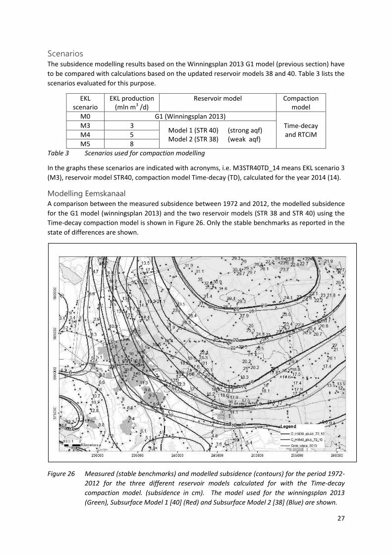
Modelling Eemskanaal
A comparison between the measured subsidence between 1972 and 2012, the modelled subsidence
for the G1 model (winningsplan 2013) and the two reservoir models (STR 38 and STR 40) using the
Time-decay compaction model is shown in Figure 26. Only the stable benchmarks as reported in the
state of differences are shown.
Figure 26 Measured (stable benchmarks) and modelled subsidence (contours) for the period 1972-
2012 for the three different reservoir models calculated for with the Time-decay
compaction model. (subsidence in cm). The model used for the winningsplan 2013
(Green), Subsurface Model 1 [40] (Red) and Subsurface Model 2 [38] (Blue) are shown.

28
The scenario with the stronger aquifer (Model 1, STR40), i.e. less pressure depletion, shows the least
subsidence. In general, modelled subsidence for this model is slightly smaller than measured
subsidence. In the scenario with the weaker aquifer (Model 2, STR38), i.e. more pressure depletion,
slightly more subsidence is modelled than measured. The subsidence calculated with the
Winningsplan 2013 model is intermediate between these scenarios. The RMS values for the different
models, calculated for the Time-decay model, are comparable (Table 4). The used of subsurface
Models 1 (STR40) and Model 2 (STR38) captures the uncertainty in the subsidence, resulting from
the uncertainty in the sub-surface model in the Eemskanaal and Groningen City Areas at the South-
West periphery of the field.
Model (time-decay) RMS
Winningsplan 1.53
Model 1 (STR 40) 1.58
Model 2 (STR 38) 1.67
Table 4 RMS values for the different models

29
Results of Compaction modelling
Figure 27 shows the total compaction volume for the two aquifer models and the G1 Winningsplan
model for both the Time-decay and RTCiM compaction model. The RTCiM model shows slightly less
compaction than the Time-decay model, which is in line with the finding that the RTCiM model
results in less subsidence than the Time-decay model. The RTCiM compaction reacts faster on
changes in the rate of pressure reduction caused by the higher production rate since 2010 (Figure
28).
Figure 27 Total compaction volume for Winningsplan (Dark blue and Red, M0) and the two sub-
surface models Model 1 (Green and Brown, 40) and Model 2 (Light blue and Purple, 38)
for the EKL base case production of 8 mln m3/day average, calculated with both the
Time-decay (TD) and RTCiM compaction models.
Figure 28 Yearly gas production of the Groningen field (2014 is YTD) (ref. NAMPLATFORM)

30
The compaction in the Eemskanaal area is calculated for both the Time-decay and RTCiM
compaction model for the year 2014 (Figure 29 and Figure 30) and for the year 2017 (Figure 31 and
Figure 32).
Figure 29; Compaction for the different models calculated with the Time-decay model for 2014, i.e.
Winningsplan (M0), weak aquifer (STR38) and the stronger aquifer (STR40)
Figure 30 Compaction for the different models calculated with the RTCiM model for 2014, i.e.
Winningsplan (M0), weak aquifer (STR38) and the stronger aquifer (STR40).

31
Figure 31 Compaction for the different models calculated with the Time Decay model for 2017, i.e.
Winningsplan (M0), weak aquifer (M4, STR38) and the stronger aquifer (M4, STR40)
Figure 32 Compaction for the different models calculated with the RTCiM model for 2017, i.e.
Winningsplan (M0), weak aquifer (M4, STR38) and the stronger aquifer (M4, STR40).
Compaction differences The additional compaction in the 3 year period 1/1/2014 to 1/1/2017 for the G1 production senario
(M0) for both the RTCiM and Time-decay compaction models is shown in Figure 33. The RTCiM
model reacts faster to changes in production and the additional compaction is approximately one cm
more than calculated with the Time-decay model. The additional compaction in this period for the
three production scenarios and two reservoir models are shown in Figure 34 for the Time-decay
compaction model and in Figure 35 for the RTCiM compaction model.

32
Time-decay RTCiM
Figure 33 Additional compaction for the G1 Winningsplan model (M0) between 2014 and 2017 for
the Time Decay and RTCiM compaction model
Figure 34 Compaction between 1/1/2014 and 1/1/2017 for the different reservoir models and
production scenarios using the Time-decay compaction model. The left column shows
the EKL production rate of 3 mln m3/d (M3), the middle column 5 mln m
3/d (M4) and the
right column 8 mln m3/d (M5). The Top row shows the weak aquifer model (STR38) and
the bottom row the stronger aquifer (STR40).

33
Figure 35 Compaction between 1/1/2014 and 1/1/2017 for the different reservoir models and
production scenarios using the RTCiM compaction model. The left column shows the EKL
production rate of 3 mln m3/d (M3), the middle column 5 mln m
3/d (M4) and the right
column 8 mln m3/d (M5). The Top row shows the weak aquifer model (STR38) and the
bottom row the stronger aquifer (STR40).

34
Seismic Response and Hazard
Methodology
Based on the compaction calculations an assessment of the hazard has been prepared for the period
winningsplan period from 1/2014 to 1/2017. The uncertainty inherent in the hazard assessment has
been assessed by a number of sensitivities.
To capture the uncertainty in the sub-surface three models are used; the G1 model used in the
update of the winningsplan 2013, the enhanced model 1 (str40) and the enhanced model 2 (str38).
The main difference between model 1 and model 2 is the assumption for the aquifers connected to
the Groningen field to the west of the Eemskanaal area of the field (ref. section Dynamic Model).
This represents the main uncertainty in the pressure distribution relevant for the hazard assessment.
Two alternative compaction models have been used; the Time-decay model developed in NAM (Ref.
1) and the RTCiM developed October last year in TNO (Ref. 3).
Also two alternative models have been developed for the assessment of induced seismicity. The
Strain Partitioning (SP) model was developed for the update of the winningsplan 2013 and has been
described in the Addendum to the winningsplan 2013 (Ref. 1). During 2014, an alternative model
was developed based on activity rates (AR). A draft report describing this model has been shared
(on 20th
October 2014) with experts in SodM, KNMI and TNO. This AR model has been
independently reviewed by an independent expert (Dr. Ian Main) and discussed at a workshop
SodM, KNMI and TNO (29th
October).
Surface accelerations were calculated using the methodology described in the Addendum to the
winningsplan 2013 (Ref. 1).
Figure 36 Two alternative seismicity models have been prepared.
The scenario table below shows the sensitivity parameters and the alternatives.
Production
Plan
Compaction
Model
Seismicity
Model
Seismic
Moment
Rates
Seismic
Activity
Rates
Gas production
schedule for
each well cluster
Spatial-temporal
distribution of
reservoir compaction
Number, magnitude,
mechanism and location
of earthquakes
Earthquake nucleation
rates depend on
reservoir strain and
past seismicity
Total seismic moment
of earthquakes
depends on reservoir
strain partitioning

35
Sub-surface
Realization Model
Compaction Model Seismicity Model Production from the
Eemskanaal Cluster
[mln Nm3/day]
Winningsplan 2013
(G1) and (M0)
Time-decay Model
(TD)
Strain Partitioning
Model
3
History match update
Model 1 (STR 40)
Rate Type Compaction
isotach Model (RTCiM)
Activity Rate Model 5
History match update
Model 2 (STR 38)
8
Figure 37 Scenario table for the hazard assessment in the Eemskanaal area.
Probabilistic Seismic Hazard Assessments Probabilistic Seismic Hazard Assessment (PSHA) is the convolution of a seismological model with a
ground motion prediction equation (GMPE) to yield the ground motion with a given probability of
exceedance at a given surface location. The PSHA results documented here pertain to all surface
locations within a 36 X 25 km region around the Eemskanaal gas production cluster. Ground motion
is measured according to the peak ground acceleration (PGA) expressed as a fraction of the
acceleration due to gravity (g). The assessment period is from 1st
January 2014 to 1st
January 2017. A
single GMPE is considered; this is identical to that used in previous assessments.
Two alternative seismological models are considered; the Strain Partitioning (SP) and the Activity
Rate (AR) models. Both seismological models are conditioned on reservoir compaction models. Two
alternative reservoir compaction models are also considered; the Time-decay (TD) and the Rate Type
Compaction Isotach (RTCiM) models. Furthermore these compaction models are conditioned on the
static and dynamic reservoir models and the future gas production plan. A wide range of alternative
cases are also considered for these as documented in Appendix Table.
These assessments are based on 105 Monte Carlo simulations of M ≥ 1.5 earthquakes and ground
motions due to M ≥ 2.5 earthquakes during the assessment period. Due to the stochastic nature of
these simulations the results remain subject to residual random variability associated with the finite
number of simulations performed. Based on the outcome of sensitivity tests residual random
variability is estimated to be approximately 0.01 g. This random variability may, in principle, be
reduced by significantly increasing the number of simulations. However, this requires significantly
more simulation time and would necessarily limit the number of alternative scenarios that could be
investigated within the time available.
The Eemskanaal gas production cluster is located at (241.539, 584.421). All map coordinates are
given as kilometers within the Dutch National triangulation coordinates system (Rijksdriehoek).
Reference Model
As a reference the hazard assessment for the Eemskanaal area was also performed for the model
and production schedule used in the update of the winningsplan 2013.
Results of the hazard assessment in Peak Ground Acceleration (PGA (g)) for the Eemskanaal area are
shown for exceedance levels of 0.2%, 2% and 10% per annum in figures 38, 39 and 40. The RCTiM
model and Strain Partitioning model have been used in this Reference Case. The RTCiM model was
not yet available when preparing the update of the winningsplan 2013 (instead the Linear Isotachen
model was used).

36
Figure 38 Hazard map showing the peak ground acceleration (PGA) with 0.2% average annual
chance of exceedance from 2014 to 2017 and the Strain Partitioning seismological
model. The contour interval is 0.05g.

37
Figure 39 Hazard map showing the peak ground acceleration (PGA) with 2% average annual
chance of exceedance from 2014 to 2017 and the Strain Partitioning seismological
model. The contour interval is 0.02g.

38
Figure 40 Hazard map showing the peak ground acceleration (PGA) with 10% average
annual chance of exceedance from 2014 to 2017 and the Strain Partitioning
seismological model. The contour interval is 0.01g.
As a reference peak ground acceleration (PGA) at the location of the Eemskanaal Cluster are 0.34 g,
0.11 g and 0.03 g for exceedance levels 0.2%, 2% and 10% respectively.
Base Case Model
As base case for this hazard assessment and associated sensitivities, the sub-surface model 1 (STR
40), the RTCiM Compaction Model and Strain Partitioning Seismogenic model were used. A
production level of 8 mln Nm3/day (see Section The Eemskanaal Cluster of Groningen) was chosen.
Results of the hazard assessment in Peak Ground Acceleration (PGA (g)) for the Eemskanaal area are
shown for exceedance levels of 0.2%, 2% and 10% per annum in figures 41, 43 and 43.

39
Figure 41 Hazard map showing the peak ground acceleration (PGA) with 0.2% average annual
chance of exceedance from 2014 to 2017 and the Strain Partitioning seismological
model. The contour interval is 0.05g.

40
Figure 42 Hazard map showing the peak ground acceleration (PGA) with 2% average annual
chance of exceedance from 2014 to 2017 and the Strain Partitioning seismological
model. The contour interval is 0.02g.


