
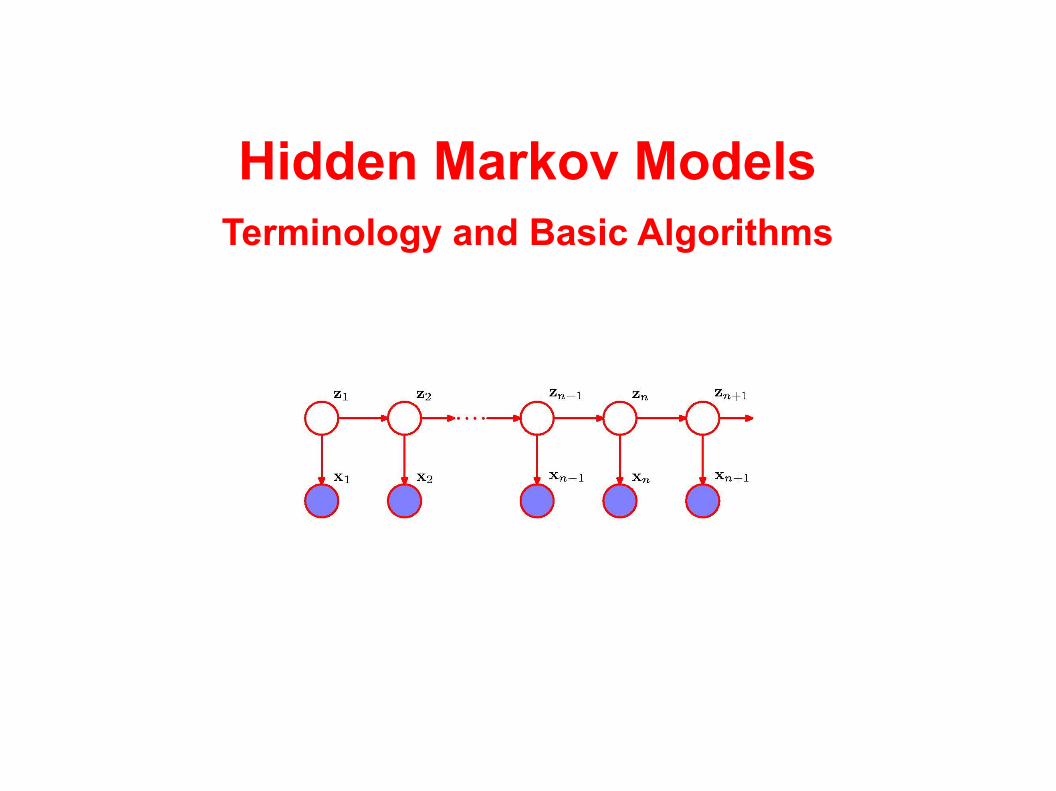
Hidden Markov ModelsTerminology and Basic Algorithms
Motivation
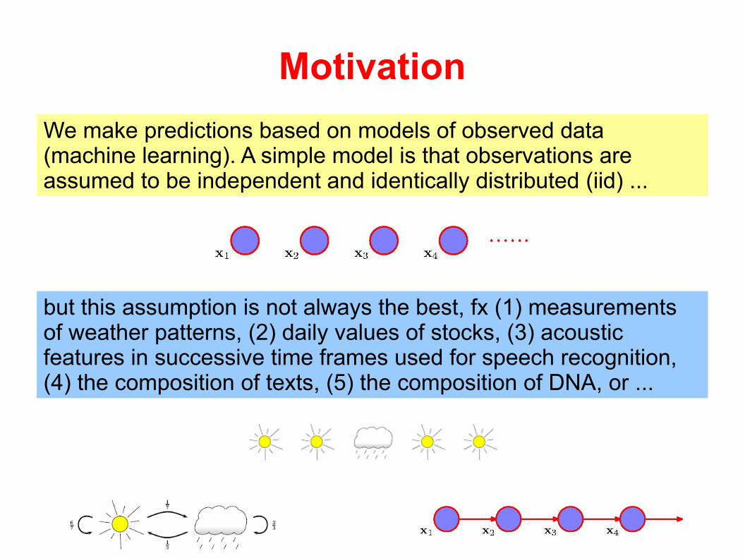
We make predictions based on models of observed data (machine learning). A simple model is that observations are assumed to be independent and identically distributed (iid) ...
but this assumption is not always the best, fx (1) measurements of weather patterns, (2) daily values of stocks, (3) acoustic features in successive time frames used for speech recognition, (4) the composition of texts, (5) the composition of DNA, or ...
Markov Models
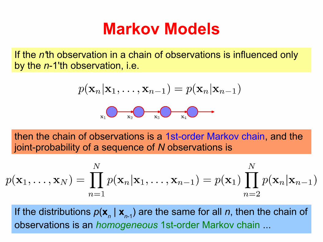
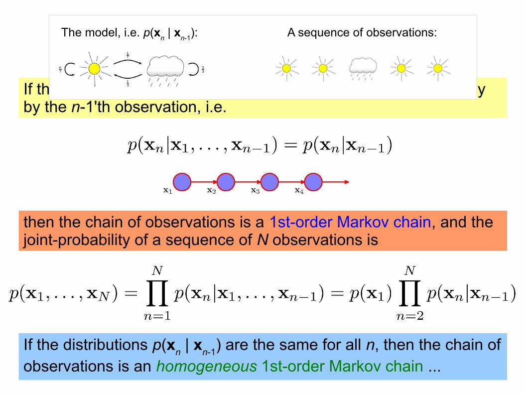
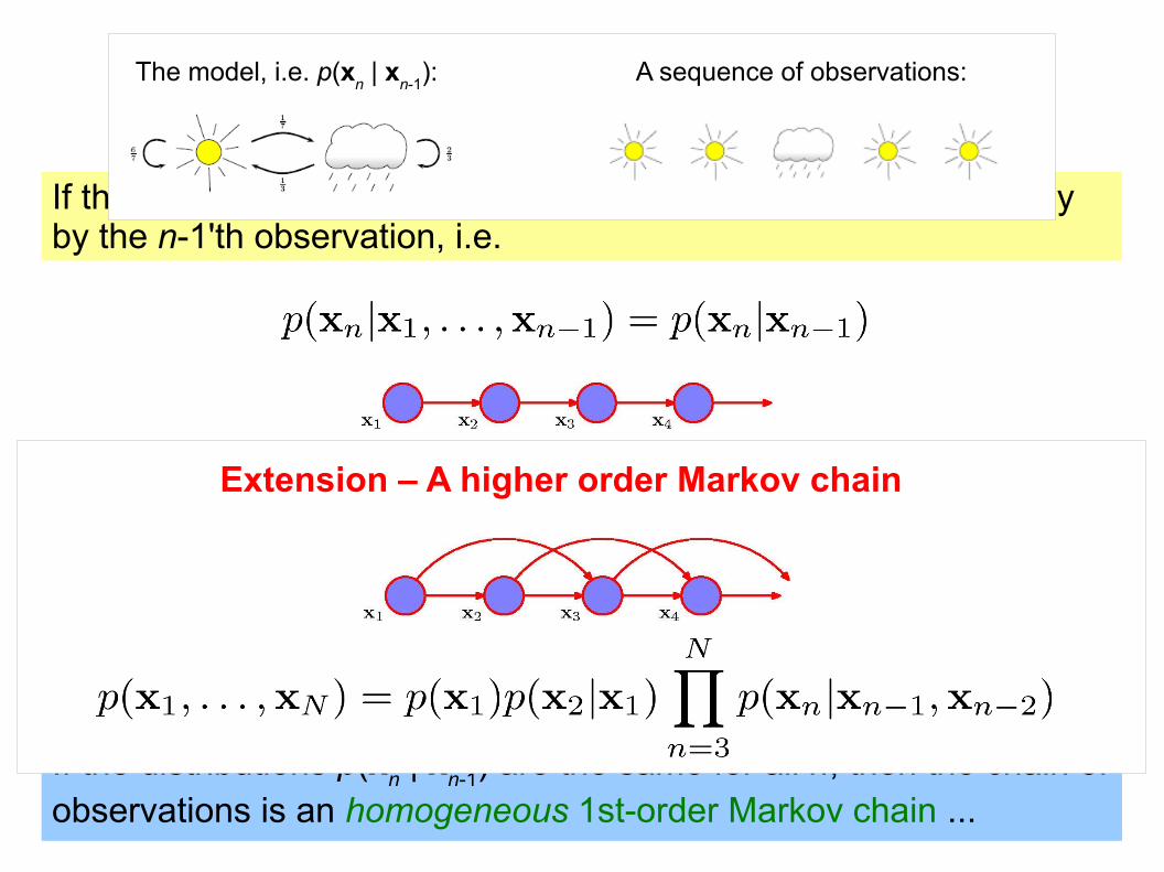
If the n'th observation in a chain of observations is influenced only by the n-1'th observation, i.e.
If the distributions p(xn | x
n-1) are the same for all n, then the chain of
observations is an homogeneous 1st-order Markov chain ...
then the chain of observations is a 1st-order Markov chain, and the joint-probability of a sequence of N observations is
Markov Models
then the chain of observations is a 1st-order Markov chain, and the joint-probability of a sequence of N observations is
If the n'th observation in a chain of observations is influenced only by the n-1'th observation, i.e.
A sequence of observations:The model, i.e. p(xn | x
n-1):
If the distributions p(xn | x
n-1) are the same for all n, then the chain of
observations is an homogeneous 1st-order Markov chain ...
If the distributions p(xn | x
n-1) are the same for all n, then the chain of
observations is an homogeneous 1st-order Markov chain ...
Markov Models
then the chain of observations is a 1st-order Markov chain, and the joint-probability of a sequence of N observations is
If the n'th observation in a chain of observations is influenced only by the n-1'th observation, i.e.
A sequence of observations:The model, i.e. p(xn | x
n-1):
Extension – A higher order Markov chain
Hidden Markov Models
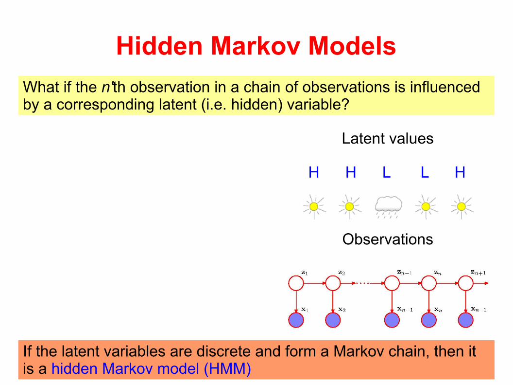
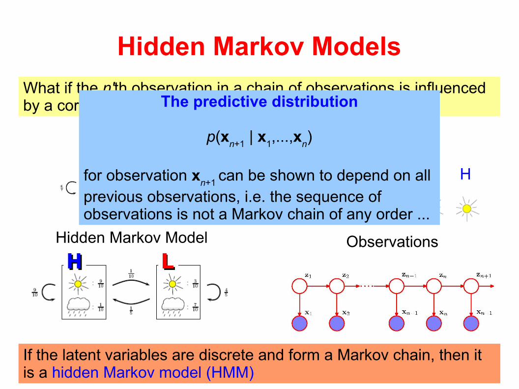
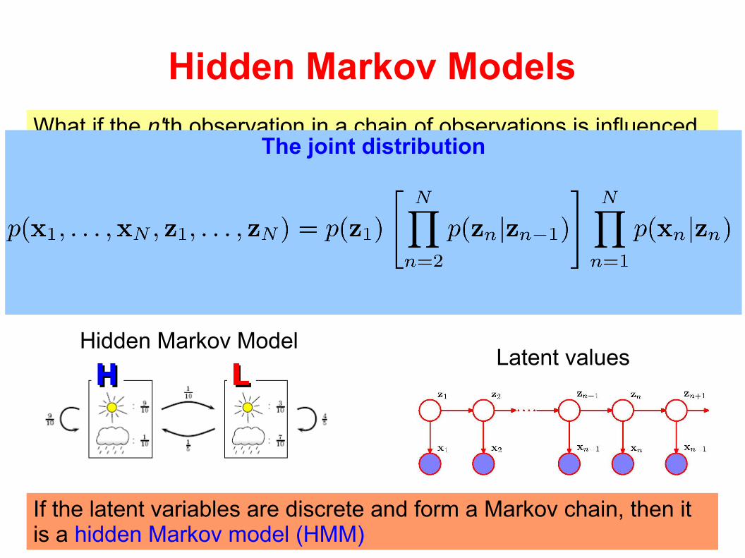
What if the n'th observation in a chain of observations is influenced by a corresponding latent (i.e. hidden) variable?
If the latent variables are discrete and form a Markov chain, then it is a hidden Markov model (HMM)
H H L L H
Observations
Latent values
Hidden Markov Models
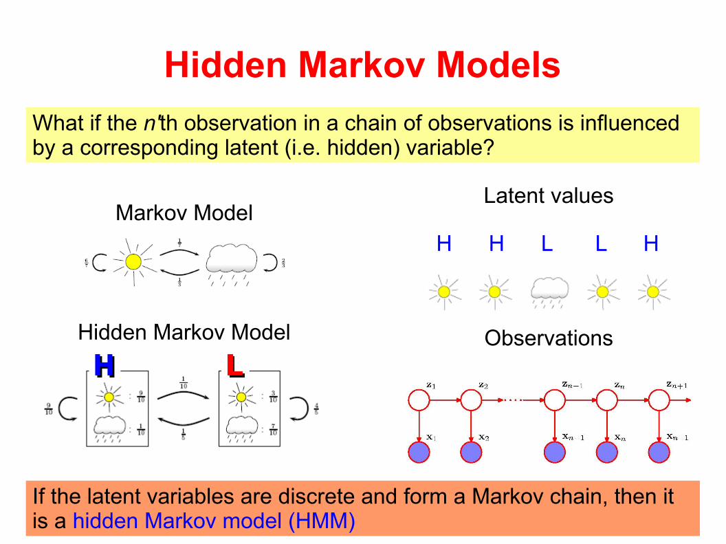
Markov Model
Hidden Markov Model
If the latent variables are discrete and form a Markov chain, then it is a hidden Markov model (HMM)
H H L L H
Observations
Latent values
What if the n'th observation in a chain of observations is influenced by a corresponding latent (i.e. hidden) variable?
Hidden Markov Models
Markov Model
Hidden Markov Model
If the latent variables are discrete and form a Markov chain, then it is a hidden Markov model (HMM)
H H L L H
Observations
Latent values
What if the n'th observation in a chain of observations is influenced by a corresponding latent (i.e. hidden) variable?
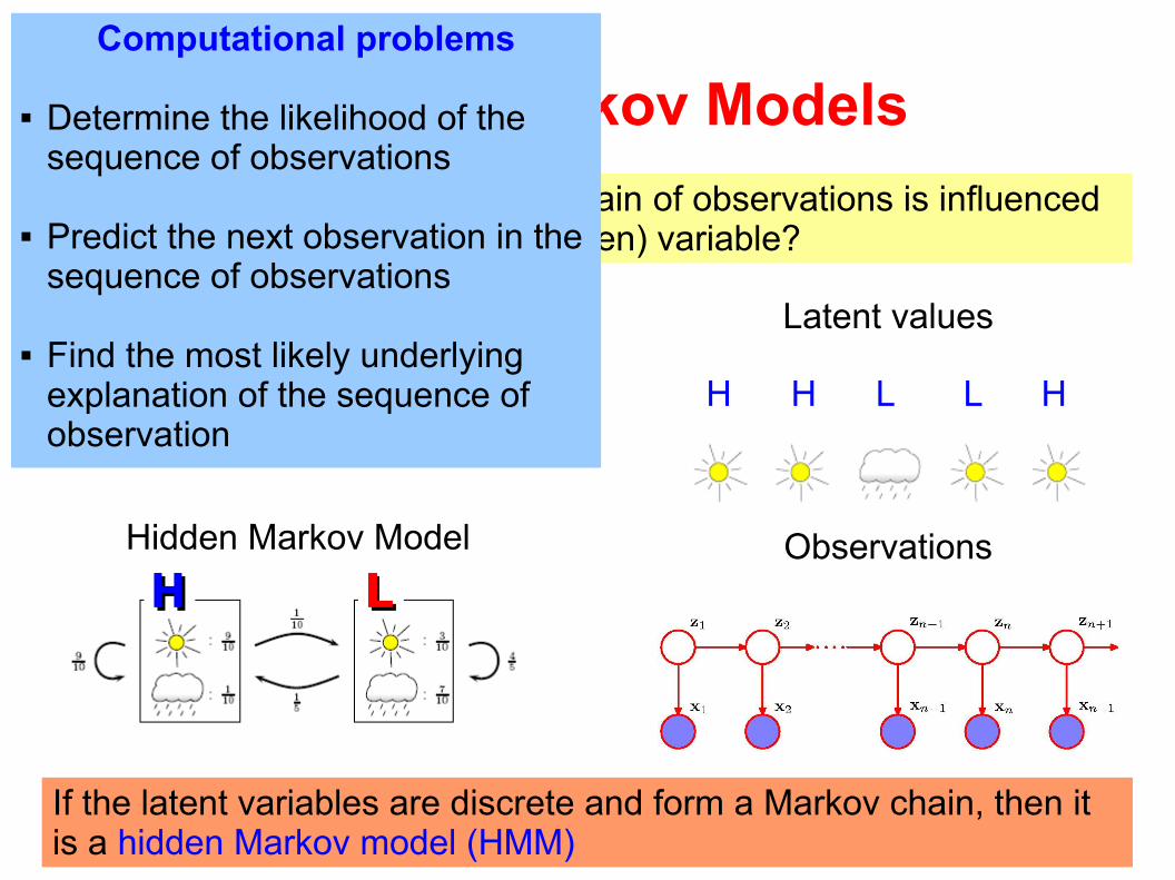
Computational problems
Determine the likelihood of the sequence of observations
Predict the next observation in the sequence of observations
Find the most likely underlying explanation of the sequence of observation
What if the n'th observation in a chain of observations is influenced by a corresponding latent (i.e. hidden) variable?
H H L L H
Observations
Latent values
Hidden Markov Models
Markov Model
Hidden Markov Model
If the latent variables are discrete and form a Markov chain, then it is a hidden Markov model (HMM)
The predictive distribution
p(xn+1
| x1,...,x
n)
for observation xn+1
can be shown to depend on all previous observations, i.e. the sequence of observations is not a Markov chain of any order ...
Hidden Markov Models
What if the n'th observation in a chain of observations is influenced by a corresponding latent variable?
Markov Model
Hidden Markov Model
H H L L H
Observations
Latent values
If the latent variables are discrete and form a Markov chain, then it is a hidden Markov model (HMM)
The joint distribution
Hidden Markov Models
What if the n'th observation in a chain of observations is influenced by a corresponding latent variable?
Markov Model
Hidden Markov Model
H H L L H
Observations
Latent values
If the latent variables are discrete and form a Markov chain, then it is a hidden Markov model (HMM)
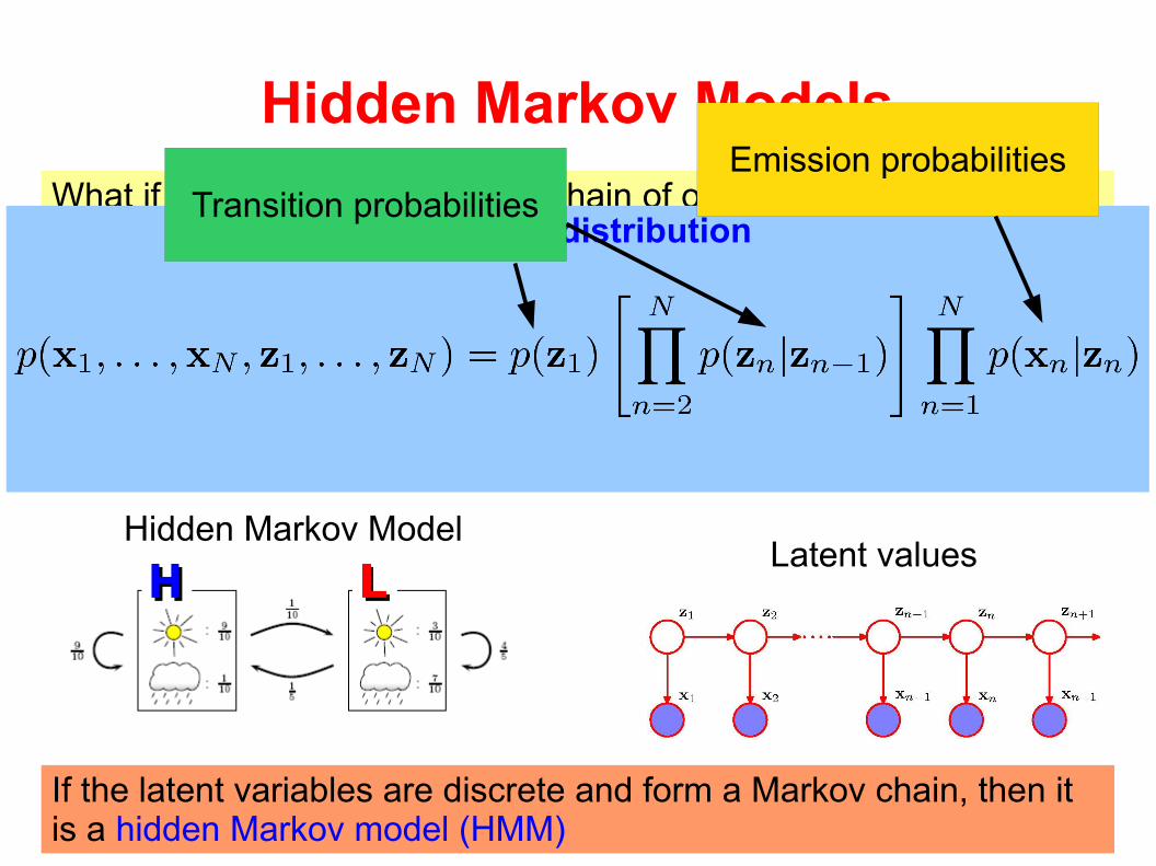
The joint distributionTransition probabilities
Emission probabilities
Transition probabilities
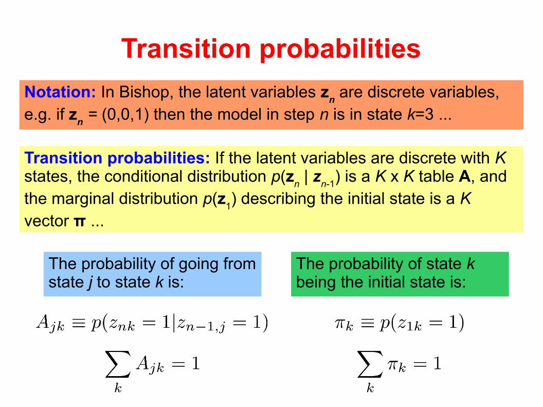
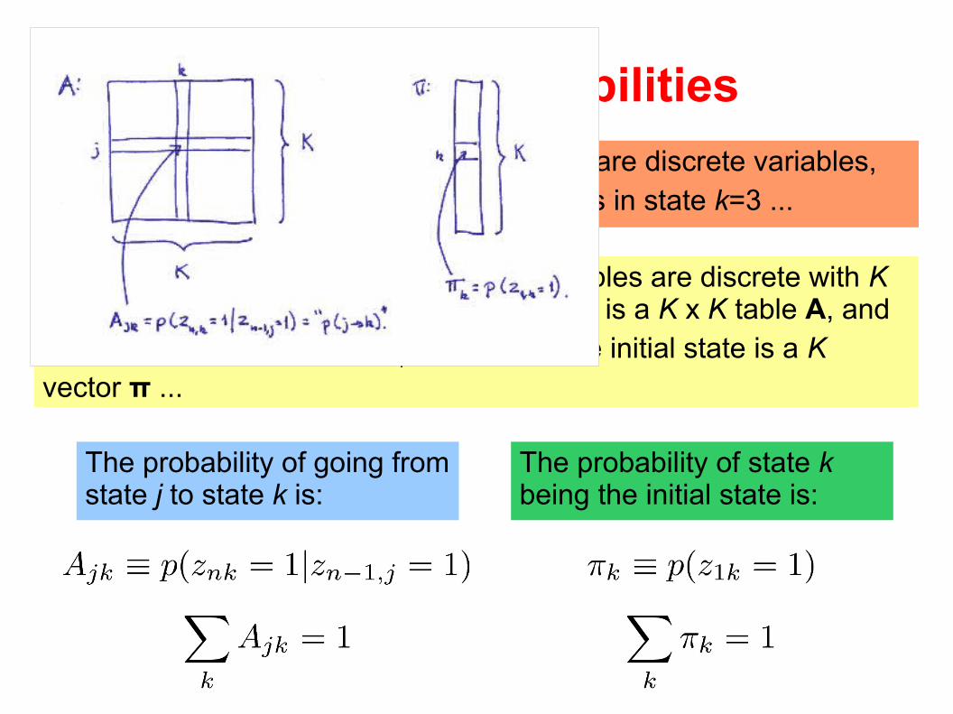
Notation: In Bishop, the latent variables zn are discrete variables,
e.g. if zn = (0,0,1) then the model in step n is in state k=3 ...
Transition probabilities: If the latent variables are discrete with K states, the conditional distribution p(z
n | z
n-1) is a K x K table A, and
the marginal distribution p(z1) describing the initial state is a K
vector π ...
The probability of going from state j to state k is:
The probability of state k being the initial state is:
Transition probabilities
Notation: In Bishop, the latent variables zn are discrete variables,
e.g. if zn = (0,0,1) then the model in step n is in state k=3 ...
Transition probabilities: If the latent variables are discrete with K states, the conditional distribution p(z
n | z
n-1) is a K x K table A, and
the marginal distribution p(z1) describing the initial state is a K
vector π ...
The probability of going from state j to state k is:
The probability of state k being the initial state is:
Transition Probabilities
Notation: The latent variables zn are discrete multinomial variables,
e.g. if zn = (0,0,1) then the model in step n is in state k=3 ...
Transition probabilities: If the latent variables are discrete with K states, the conditional distribution p(z
n | z
n-1) is a K x K table A, and
the marginal distribution p(z1) describing the initial state is a K
vector π ...
The probability of going from state j to state k is:
The probability of state k being the initial state is:
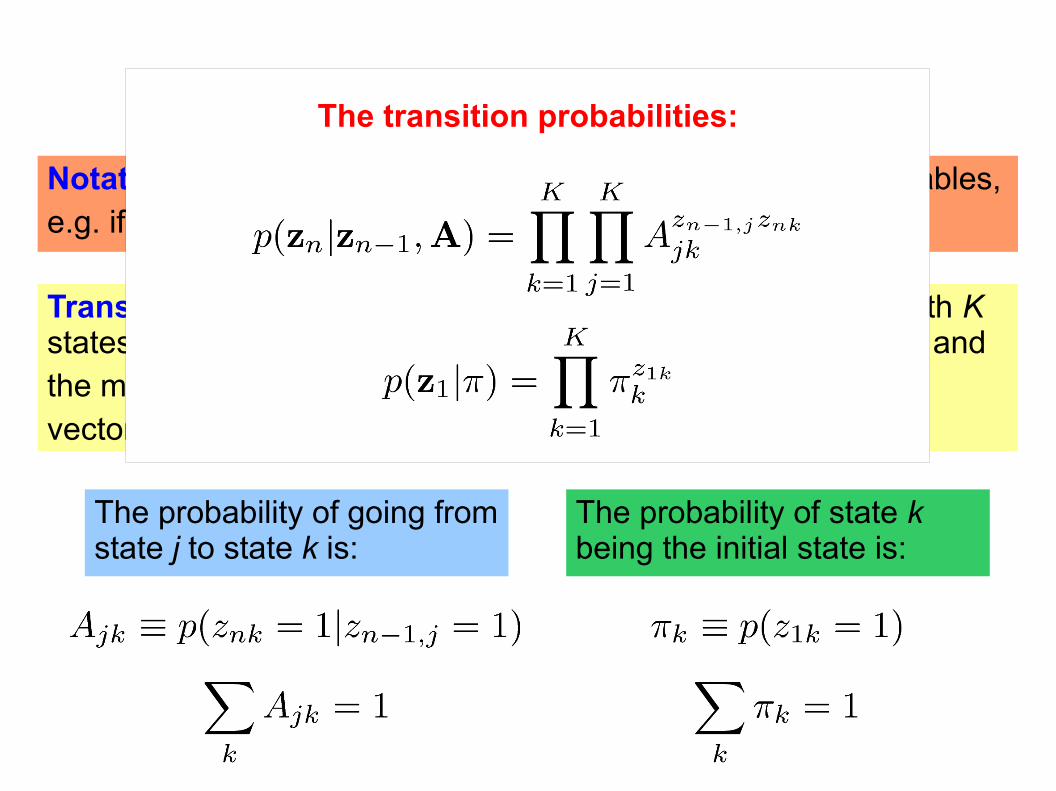
The transition probabilities:
Transition Probabilities
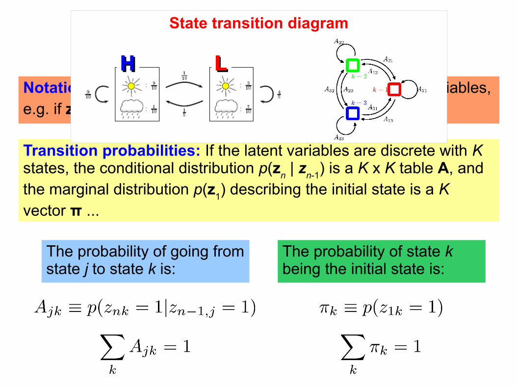
Notation: The latent variables zn are discrete multinomial variables,
e.g. if zn = (0,0,1) then the model in step n is in state k=3 ...
Transition probabilities: If the latent variables are discrete with K states, the conditional distribution p(z
n | z
n-1) is a K x K table A, and
the marginal distribution p(z1) describing the initial state is a K
vector π ...
State transition diagram
The probability of going from state j to state k is:
The probability of state k being the initial state is:
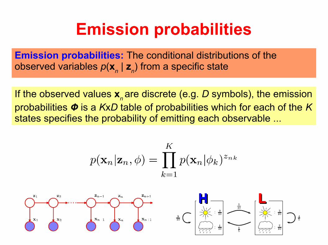
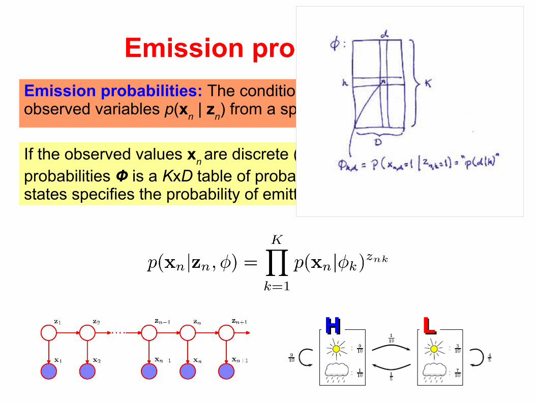
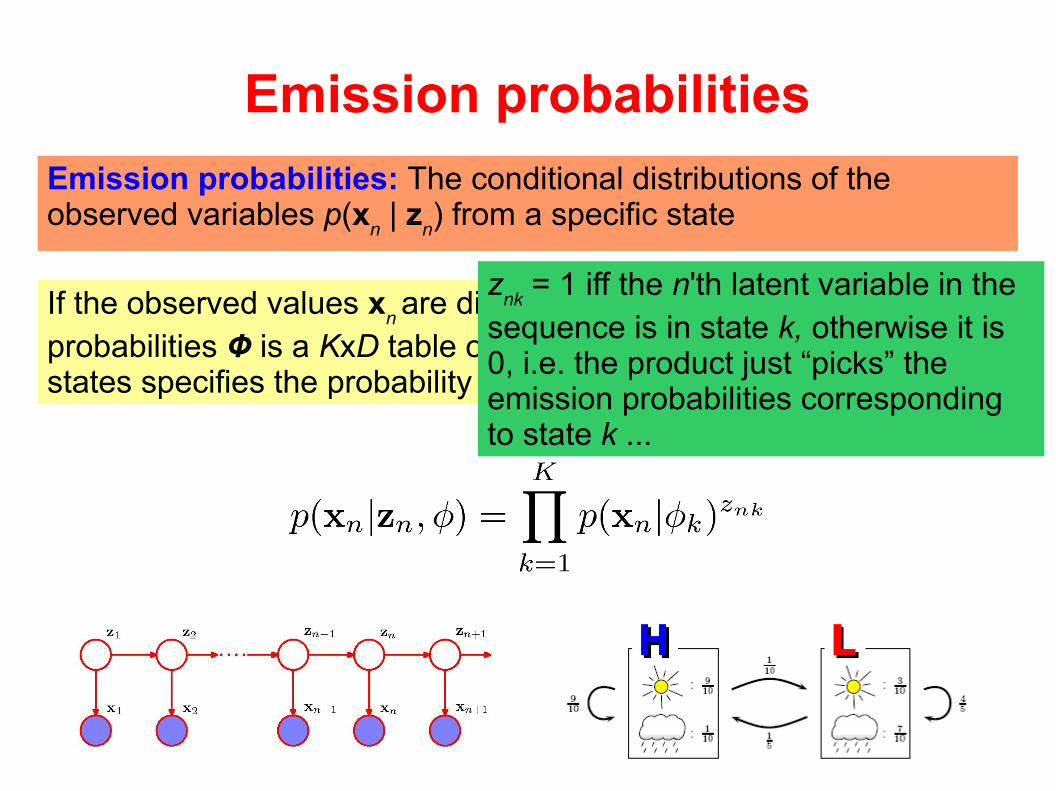
Emission probabilities
Emission probabilities: The conditional distributions of the observed variables p(x
n | z
n) from a specific state
If the observed values xn are discrete (e.g. D symbols), the emission
probabilities Ф is a KxD table of probabilities which for each of the K states specifies the probability of emitting each observable ...
znk
= 1 iff the n'th latent variable in the sequence is in state k, otherwise it is 0, i.e. the product just “picks” the emission probabilities corresponding to state k ...
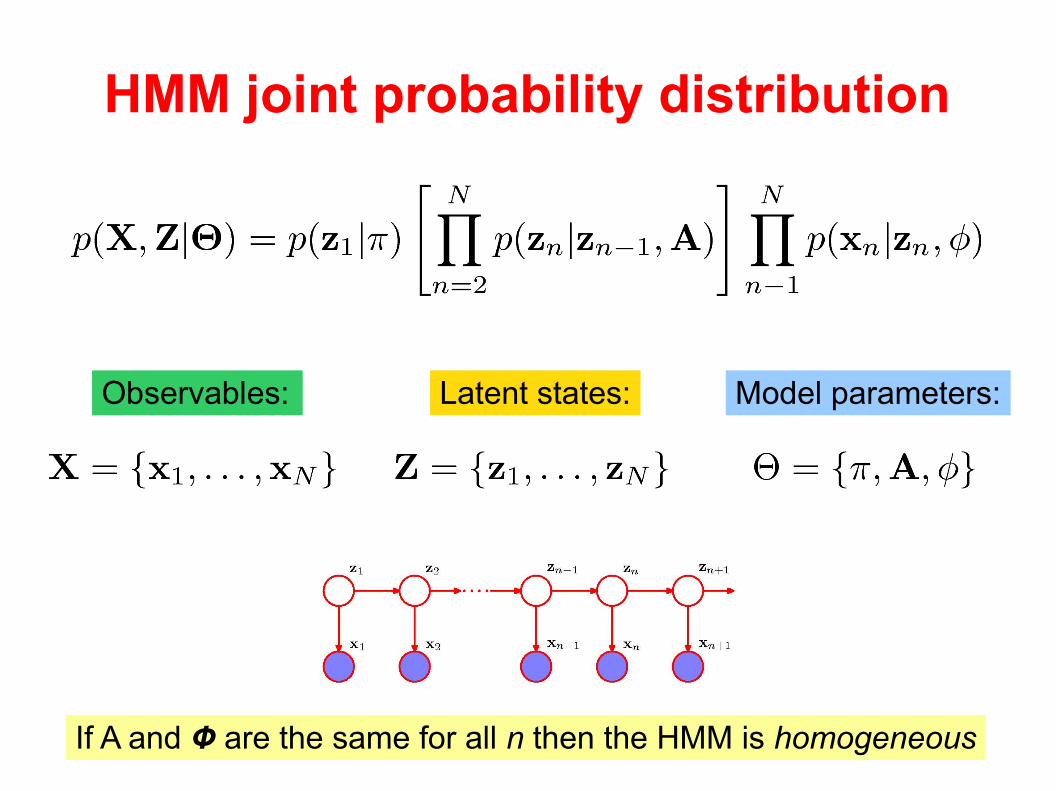
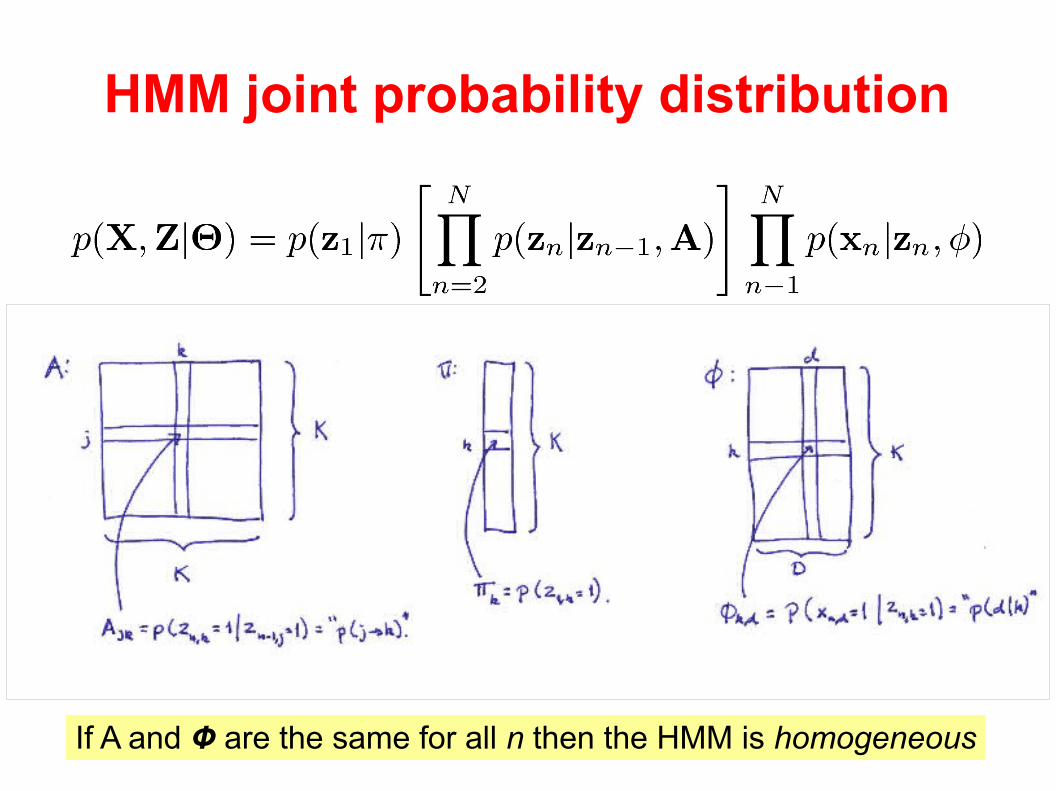
HMM joint probability distribution
If A and Ф are the same for all n then the HMM is homogeneous
Observables: Latent states: Model parameters:
HMM joint probability distribution
If A and Ф are the same for all n then the HMM is homogeneous
Observables: Latent states: Model parameters:
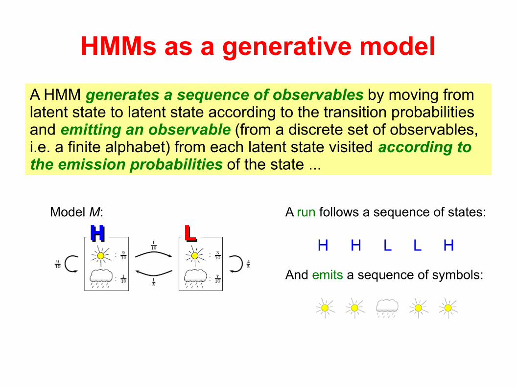
HMMs as a generative model
Model M: A run follows a sequence of states:
H H L L H
And emits a sequence of symbols:
A HMM generates a sequence of observables by moving from latent state to latent state according to the transition probabilities and emitting an observable (from a discrete set of observables, i.e. a finite alphabet) from each latent state visited according to the emission probabilities of the state ...
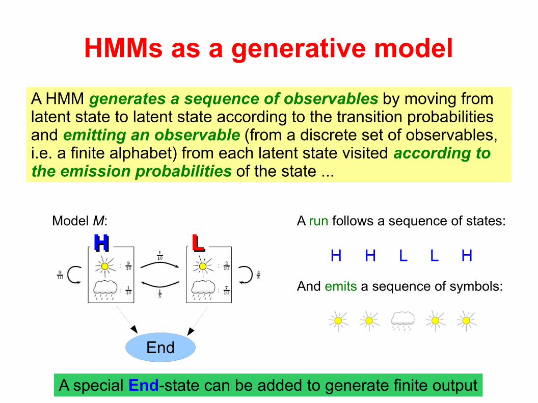
HMMs as a generative model
End
A special End-state can be added to generate finite output
Model M: A run follows a sequence of states:
H H L L H
And emits a sequence of symbols:
A HMM generates a sequence of observables by moving from latent state to latent state according to the transition probabilities and emitting an observable (from a discrete set of observables, i.e. a finite alphabet) from each latent state visited according to the emission probabilities of the state ...
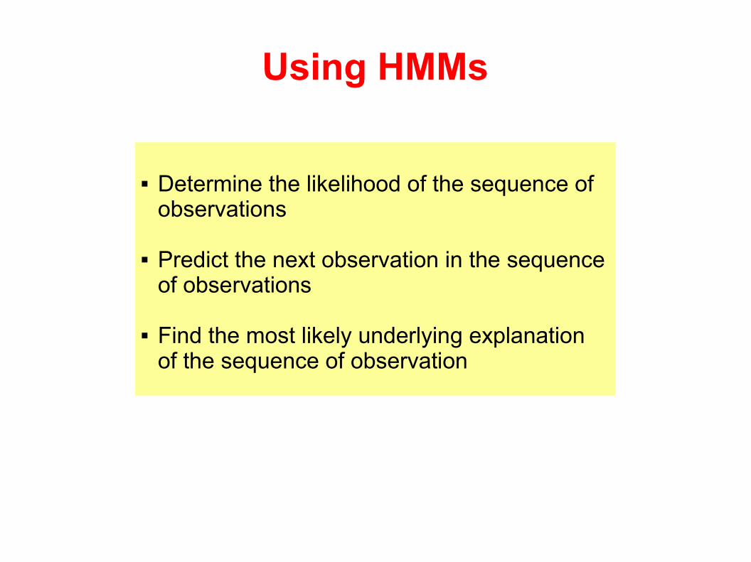
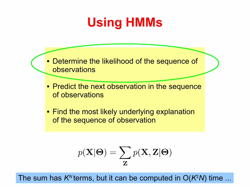
Using HMMs
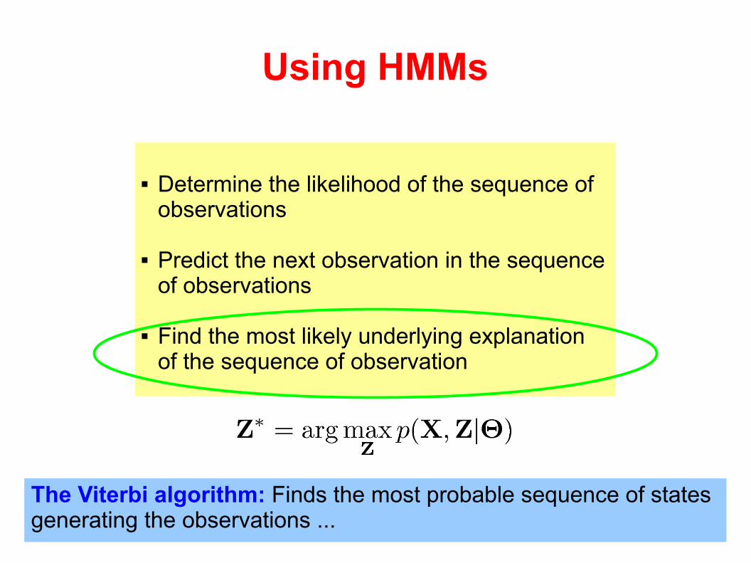
Determine the likelihood of the sequence of observations
Predict the next observation in the sequence of observations
Find the most likely underlying explanation of the sequence of observation
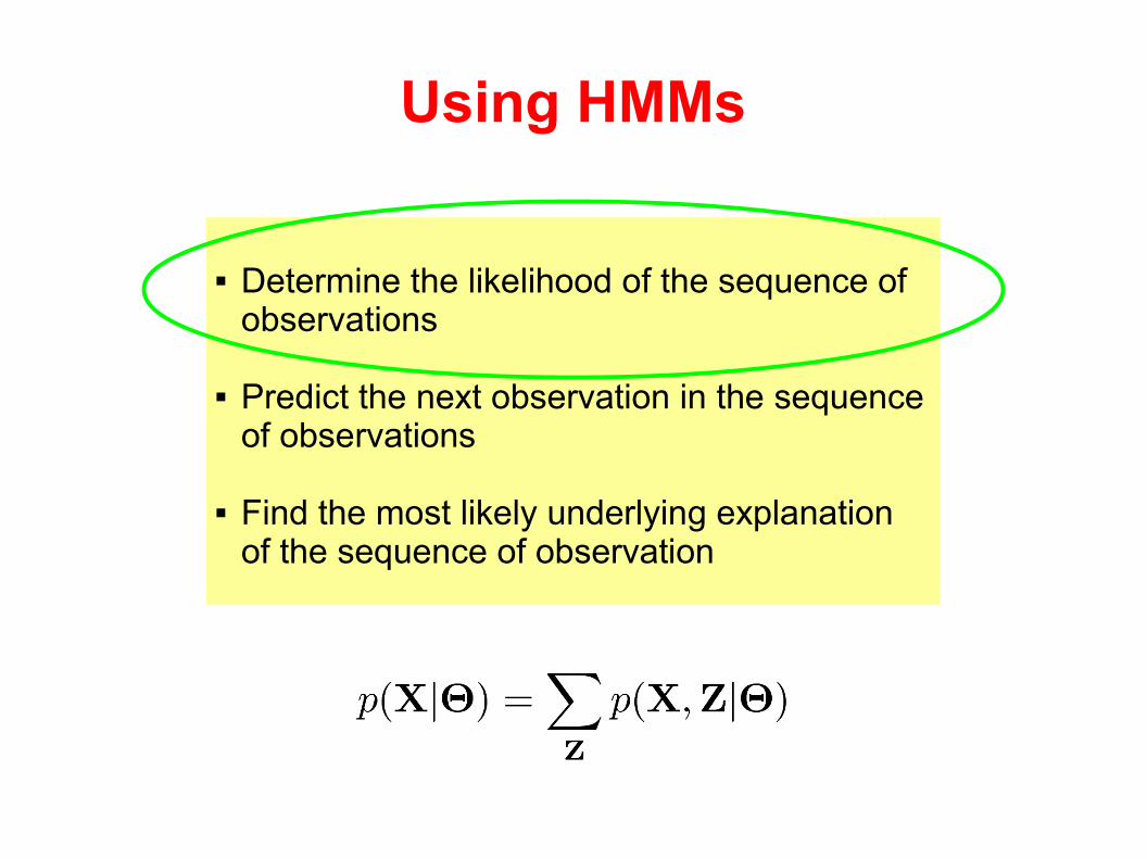
Using HMMs
Determine the likelihood of the sequence of observations
Predict the next observation in the sequence of observations
Find the most likely underlying explanation of the sequence of observation
Using HMMs
Determine the likelihood of the sequence of observations
Predict the next observation in the sequence of observations
Find the most likely underlying explanation of the sequence of observation
The sum has KN terms, but it can be computed in O(K2N) time ...
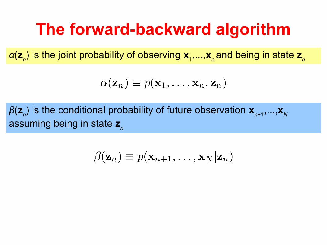
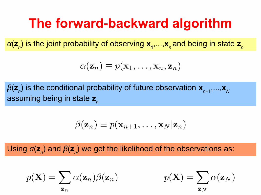
The forward-backward algorithm
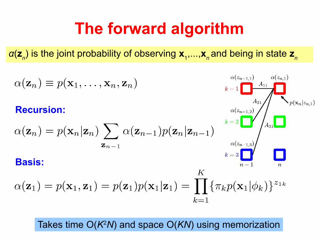
α(zn) is the joint probability of observing x
1,...,x
n and being in state z
n
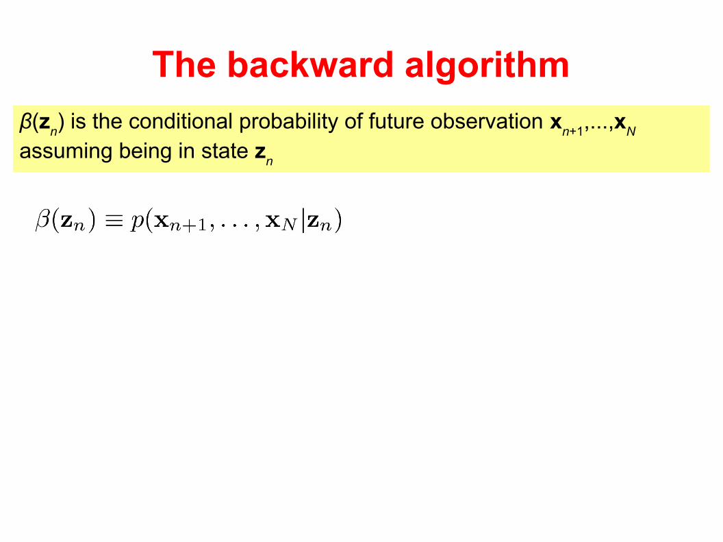
β(zn) is the conditional probability of future observation x
n+1,...,x
N
assuming being in state zn
α(zn) is the joint probability of observing x
1,...,x
n and being in state z
n
β(zn) is the conditional probability of future observation x
n+1,...,x
N
assuming being in state zn
Using α(zn) and β(z
n) we get the likelihood of the observations as:
The forward-backward algorithm
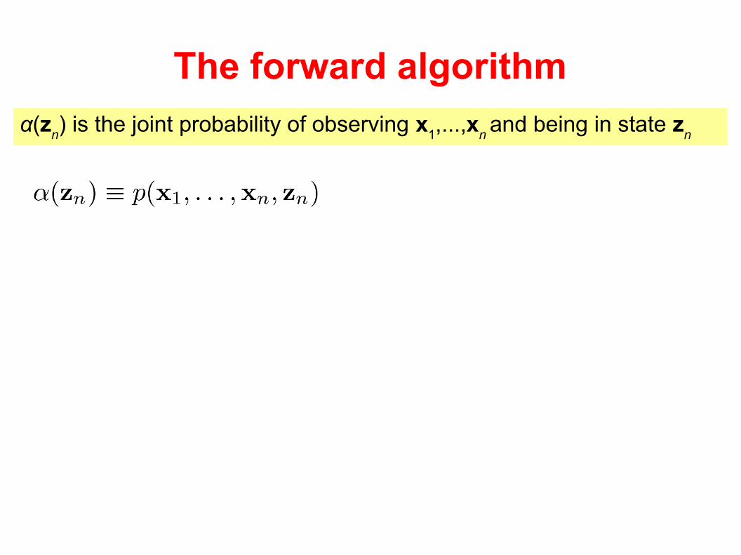
The forward algorithm
α(zn) is the joint probability of observing x
1,...,x
n and being in state z
n
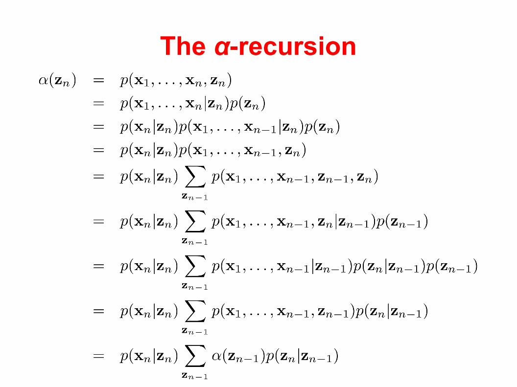
The α-recursion
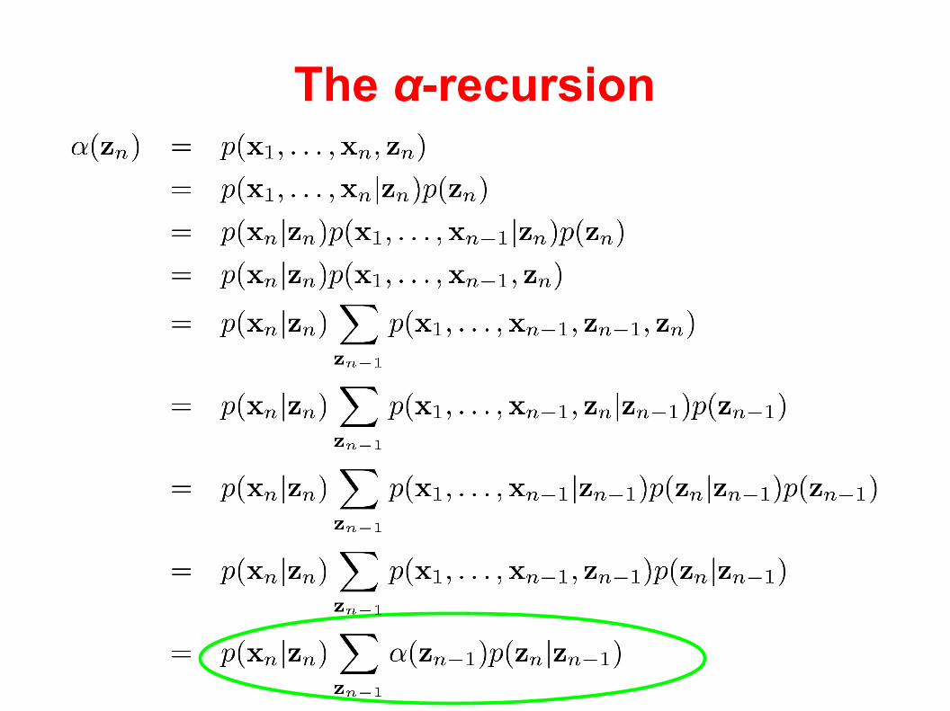
The α-recursion
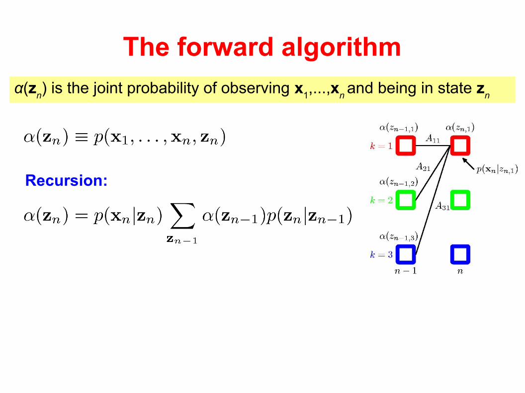
The forward algorithm
α(zn) is the joint probability of observing x
1,...,x
n and being in state z
n
Recursion:
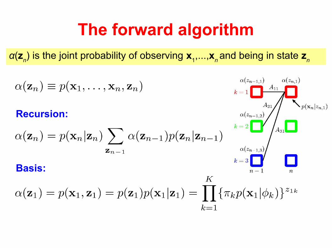
The forward algorithm
α(zn) is the joint probability of observing x
1,...,x
n and being in state z
n
Recursion:
Basis:
The forward algorithm
α(zn) is the joint probability of observing x
1,...,x
n and being in state z
n
Recursion:
Basis:
Takes time O(K2N) and space O(KN) using memorization
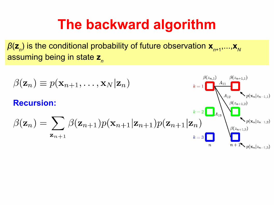
The backward algorithm
β(zn) is the conditional probability of future observation x
n+1,...,x
N
assuming being in state zn
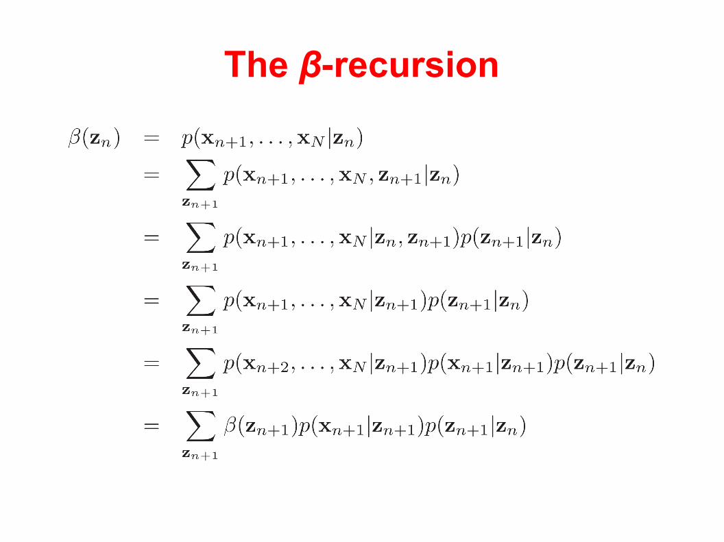
The β-recursion
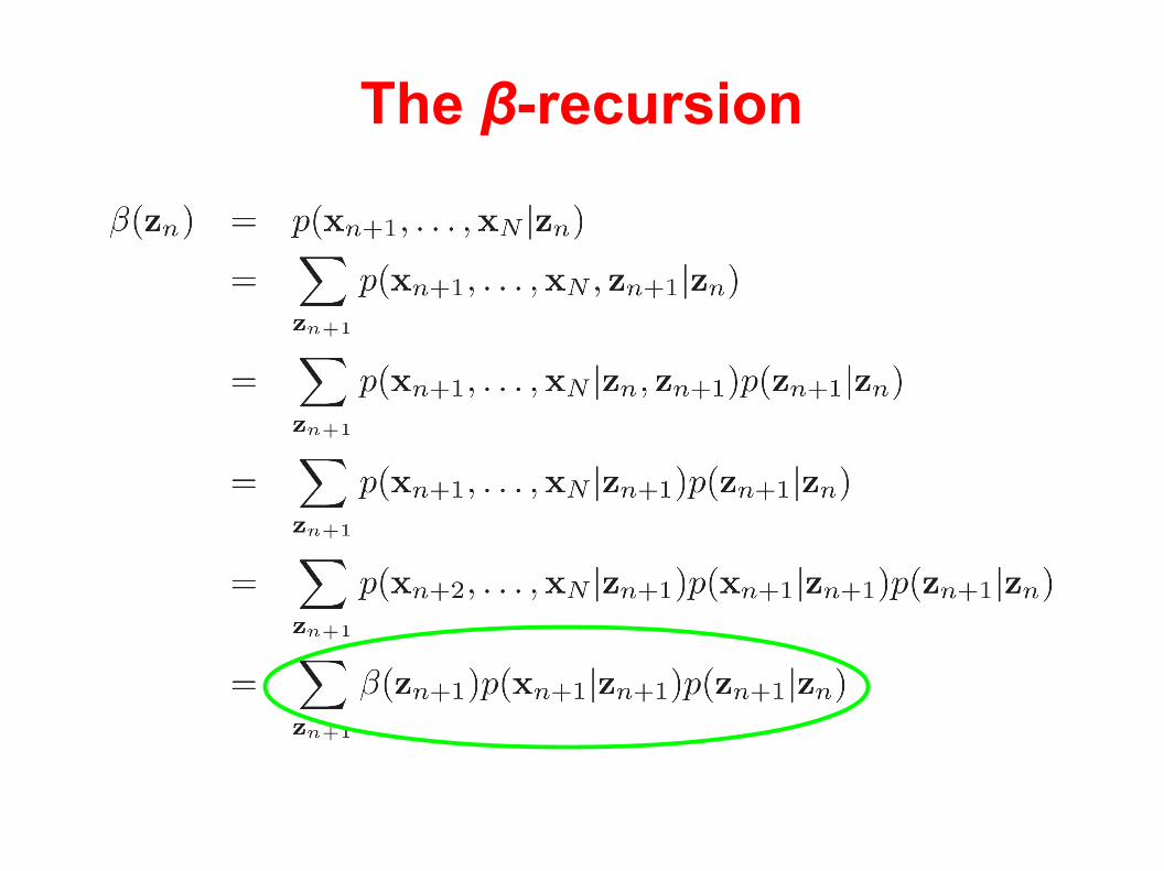
The β-recursion
The backward algorithm
Recursion:
β(zn) is the conditional probability of future observation x
n+1,...,x
N
assuming being in state zn
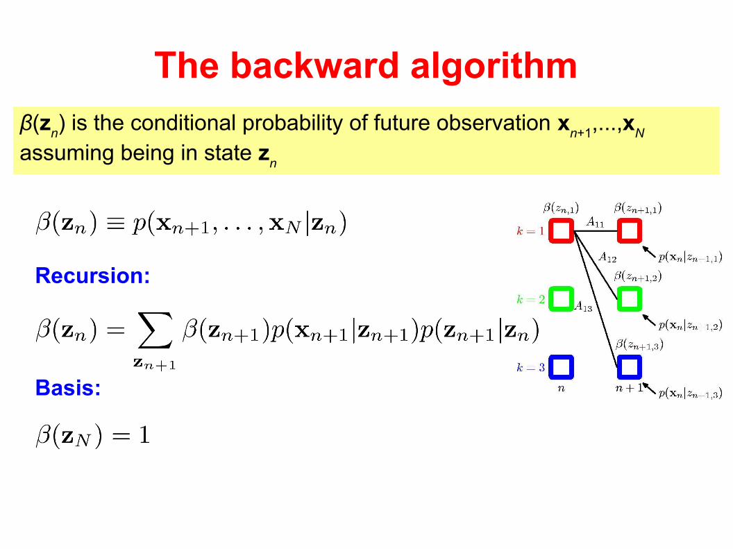
The backward algorithm
Recursion:
Basis:
β(zn) is the conditional probability of future observation x
n+1,...,x
N
assuming being in state zn
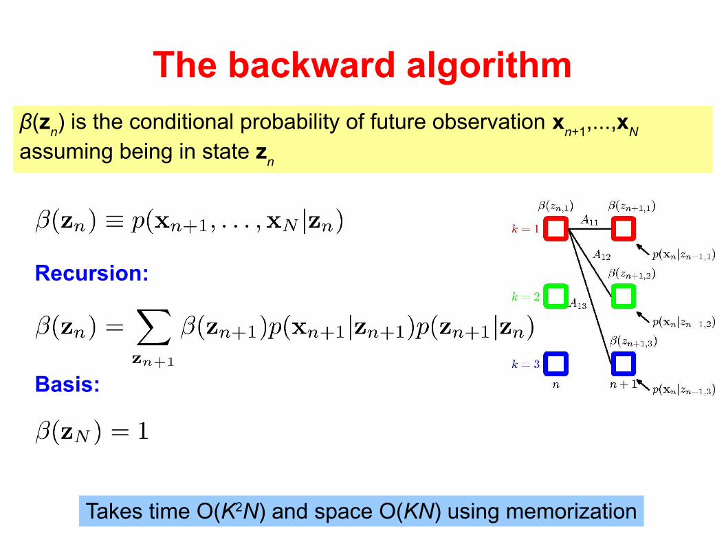
The backward algorithm
β(zn) is the conditional probability of future observation x
n+1,...,x
N
assuming being in state zn
Recursion:
Basis:
Takes time O(K2N) and space O(KN) using memorization
Determine the likelihood of the sequence of observations
Predict the next observation in the sequence of observations
Find the most likely underlying explanation of the sequence of observation
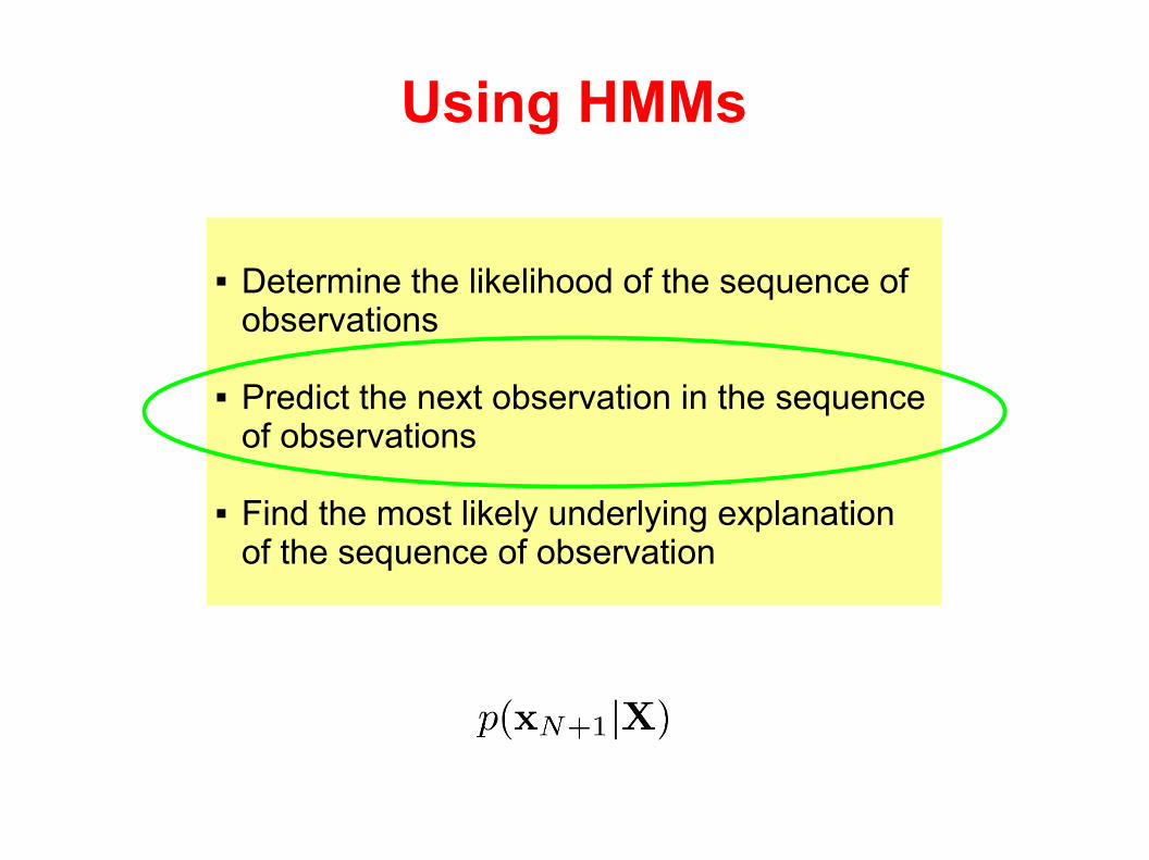
Using HMMs
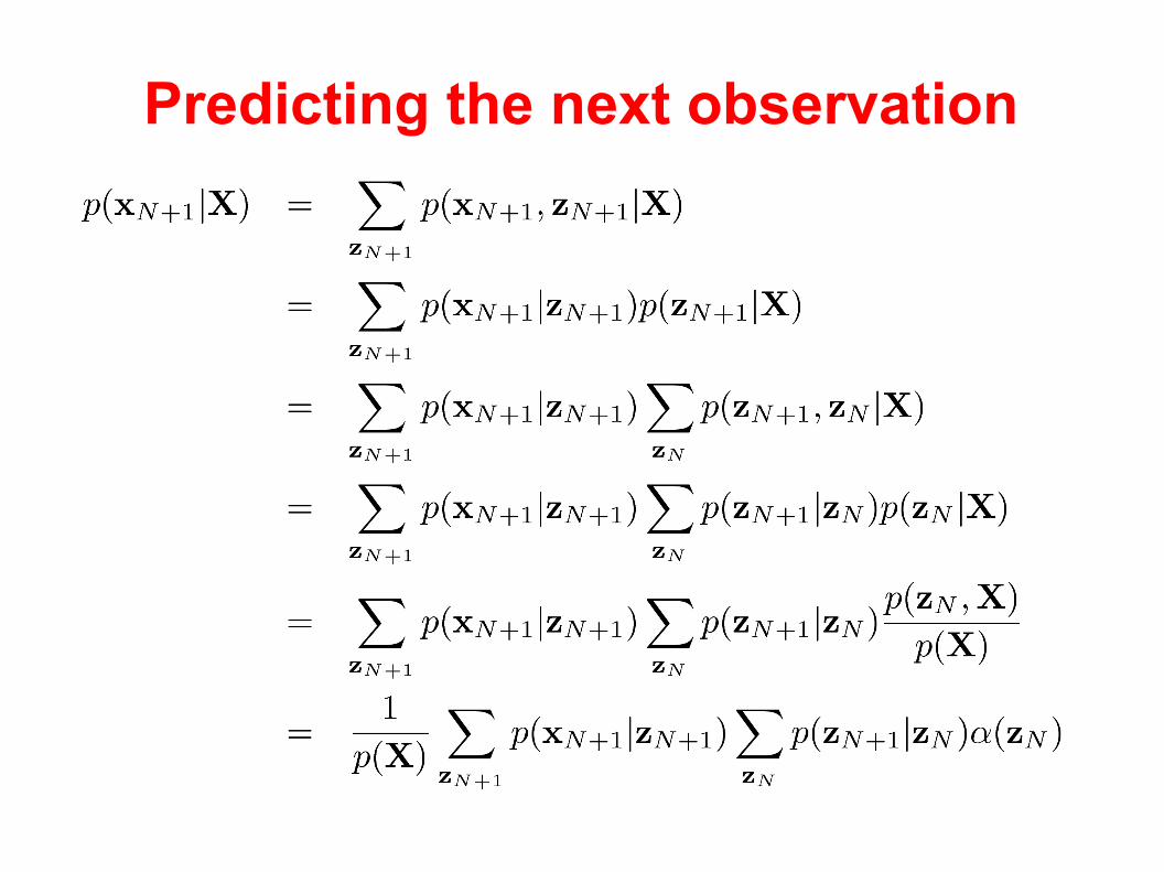
Predicting the next observation
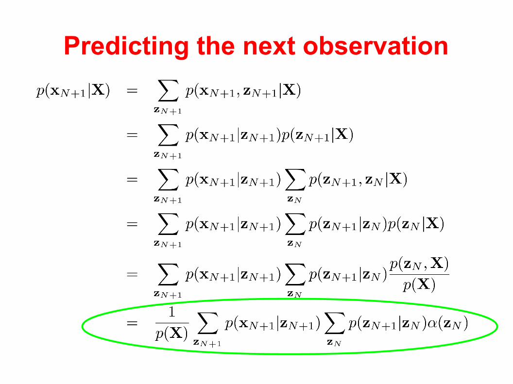
Predicting the next observation
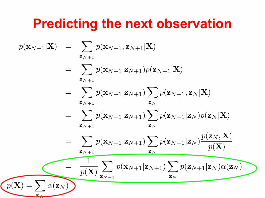
Predicting the next observation
Determine the likelihood of the sequence of observations
Predict the next observation in the sequence of observations
Find the most likely underlying explanation of the sequence of observation
Using HMMs
The Viterbi algorithm: Finds the most probable sequence of states generating the observations ...
The Viterbi algorithm
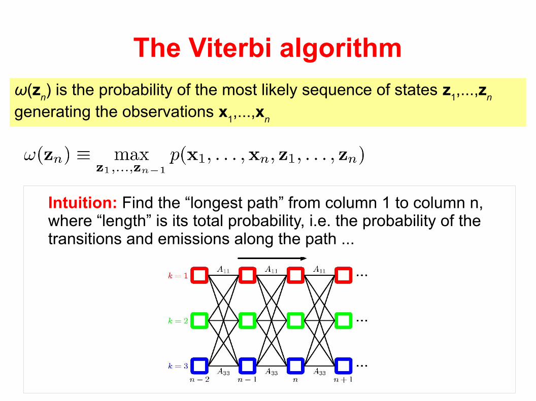
ω(zn) is the probability of the most likely sequence of states z
1,...,z
n
generating the observations x1,...,x
n
h
Intuition: Find the “longest path” from column 1 to column n, where “length” is its total probability, i.e. the probability of the transitions and emissions along the path ...
The Viterbi algorithm
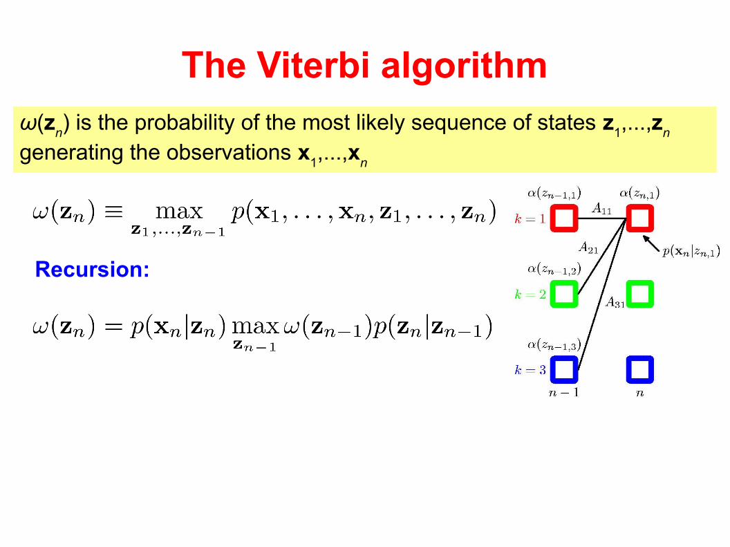
ω(zn) is the probability of the most likely sequence of states z
1,...,z
n
generating the observations x1,...,x
n
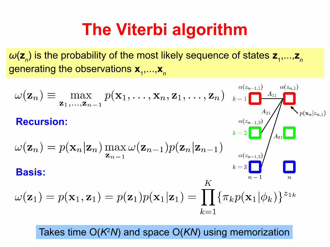
Recursion:
The Viterbi algorithm
ω(zn) is the probability of the most likely sequence of states z
1,...,z
n
generating the observations x1,...,x
n
Recursion:
Basis:
Takes time O(K2N) and space O(KN) using memorization
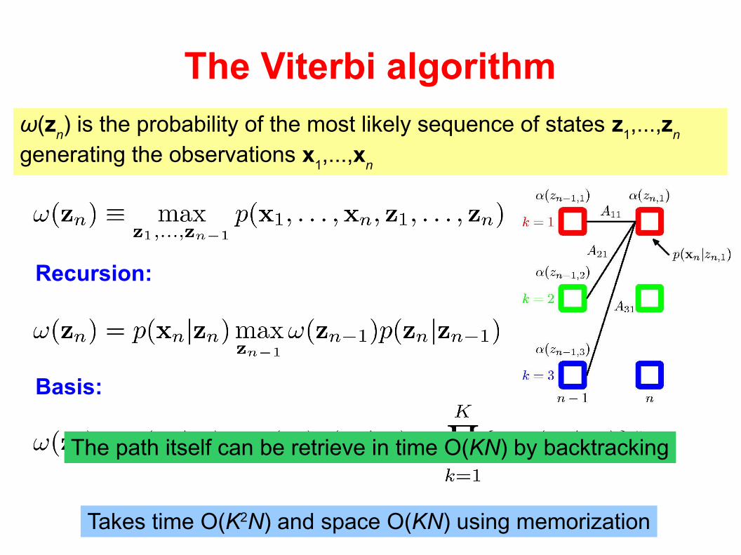
ω(zn) is the probability of the most likely sequence of states z
1,...,z
n
generating the observations x1,...,x
n
Recursion:
Basis:
Takes time O(K2N) and space O(KN) using memorization
The path itself can be retrieve in time O(KN) by backtracking
The Viterbi algorithm
Summary
Introduced hidden Markov models (HMMs)
The forward-backward algorithms for determining the likelihood of a sequence of observations, and predicting the next observation in a sequence of observations.
The Viterbi-algorithm for finding the most likely underlying explanation (sequence of latent states) of a sequence of observation
Next: How to implement the basic algorihtms (forward, backward, and Viterbi) in a “numerically” sound manner.


