

ISSN 1178-2293 (Online)
University of Otago Economics Discussion Papers
No. 1307
April 2013
How Much Does Women’s Empowerment Influence
their Wellbeing? Evidence from Africa
David Fielding University of Otago
Address for correspondence: David Fielding Department of Economics University of Otago PO Box 56 Dunedin NEW ZEALAND Email: [email protected] Telephone: 64 3 479 8653
1
How Much Does Women’s Empowerment Influence their
Wellbeing? Evidence from Africa
David Fielding§
Abstract
One of the eight Millennium Development Goals is to ‘promote gender equality and empower women.’
However, only 1% of official foreign aid is currently spent on gender equality and human rights. Using
individual-level survey data from 39 villages in northern Senegal, we model the effects that freedom
within the home have on married women’s subjective wellbeing. We find the direct effects on wellbeing
to be of a similar magnitude to the direct effects of consumption, education and morbidity. These results
suggest the need for a review of aid allocation priorities.
JEL classification: O15; J12; I15
Keywords: wellbeing; health; women’s empowerment
§ Address for correspondence: Department of Economics, University of Otago, Dunedin 9054, New Zealand. E-mail
[email protected]; telephone +6434798653.
2
1. Introduction
International evidence suggests that the positive correlation between women’s rights and other
dimensions of human development at the macroeconomic level is driven by causal effects in both
directions (Doepke et al., 2012). In this sense, the empowerment of women is an integral part of the
development process. Correspondingly, one of the eight Millennium Development Goals – MDG3 – is
to ‘promote gender equality and empower women.’ However, progress towards this goal has been slow:
according to the United Nations (2013), ‘Gender inequality persists and women continue to face
discrimination in access to education, work and economic assets.’ Bilateral and multilateral donors have
begun to allocate some foreign aid to the promotion of gender equality and human rights, but this type of
aid still only makes up 1% of the total worldwide aid budget.1
In this paper, we use survey data from rural Senegal to model the effects on married women’s
subjective wellbeing of the amount of freedom they have in the home. Senegal has a democratically
elected government which broadly supports human rights and women’s empowerment, but this contrasts
with conservative attitudes towards women in some traditional rural communities. Our data reveals
substantial variation in the treatment of women, and we find the effect of this variation on women’s
wellbeing to be large when compared with the direct effects of more traditional development goals, such
as raising consumption and education, or lowering morbidity. This result suggests a reassessment of the
current allocation of foreign aid, with more emphasis to expenditure on women’s empowerment, and
more concern about the interaction of empowerment with other dimensions of development.2 The next
1 Figures in the OECD-DAC database (www.oecd.org/dac/stats) indicate that in 2011, total official aid to all recipients
was $159bn, of which aid for human rights and women’s equality organisations (sectors 15160 and 15170) was
$1.58bn. The corresponding figures for Senegal are $913mn and $1.65mn. 2 We do not mean to imply that women’s rights are of value only to the extent that they contribute to women’s utility:
rights could also have an intrinsic value (Sen, 1991). But even if ones assumes that this intrinsic value is zero, our
results still suggest that the overall value of women’s rights is overlooked in current foreign aid allocations.

3
section reviews the literature on women’s empowerment and wellbeing; this is followed by a discussion
of the data, and then the econometric model.
2. Literature Review
If husbands and wives have different preferences, and if the husband is not entirely altruistic, then in a
male-dominated society there is an incentive for the husband to impose his will on his wife (or wives).
The ability of wives to resist this pressure will depend on their bargaining power. With more bargaining
power, women will be able to negotiate an allocation of household resources that is better for them (or
for their children) in terms of what they consume and how their time is spent. Women’s empowerment
might also affect the form that bargaining takes: for example, it might limit violent behavior by the
husband. Evidence for the existence of intra-household bargaining in developing countries appears in
numerous econometric studies, many of which are summarized in Doss (2013). Some authors use
statistical analysis of survey data to measure the effect on households of natural experiments involving
exogenous changes that can reasonably be assumed to have increased female bargaining power.
Examples of such natural experiments include changes in marriage or inheritance laws (Deininger et al.,
2010; Rangel, 2006) and shocks to gender-specific income (Duflo, 2003; Qian, 2008). Positive shocks to
female bargaining power are found to improve child education or child health, which suggests that on
average mothers value their children more than fathers do. Other authors find similar results by using
Instrumental Variables estimators to analyze changes in conditions which affect bargaining power but
might not be exogenous (Brown, 2003; Doss, 2001; Duflo and Udry, 2004). There is also some evidence
for intra-household bargaining effects from experimental studies. Field studies involving gender-specific
cash transfer programs show that transfers to women are more beneficial to children, on average, than
are transfers to men (Behrman and Hoddinott, 2005; Bobonis, 2009; Lim et al., 2010; Maluccio and
4
Flores, 2005),3 while experimental games between husbands and wives show that treatments changing
one spouse’s bargaining power can have a large effect on outcomes (Ashraf, 2009; Iversen et al., 2006).
In all of these studies (with the possible exception of the experimental games), women’s
empowerment is a latent variable that is not measured explicitly. It is therefore difficult to use the results
to quantify the overall effect of empowerment on household outcomes and on women’s wellbeing.
However, there is an epidemiological literature in which empowerment is measured explicitly, and the
effect of empowerment on health outcomes is estimated directly. Here, empowerment is measured using
survey data on women’s decision-making power within the home. Respondents – either husbands or
wives, or both – indicate who has a say in a range of household choices, for example decisions about
household purchases, or whether the wife goes to seek formal healthcare, or whether she is allowed to
make visits to her relatives. Women are taken to be most empowered when they make these decisions
alone, and least empowered when their husband makes these decisions alone. Several papers (for
example Allendorf, 2007, 2010; Furuta and Salway, 2006; Lépine, 2012; Mistry et al., 2009) find strong
evidence that these indicators of empowerment are positively correlated with health outcomes such as
access to antenatal care, delivery of children in hospital, child nutrition, or vaccination against common
infectious diseases. However, this evidence is mostly concentrated on the Indian subcontinent, and the
focus of attention is entirely on specific health outcomes rather than on general wellbeing. Another
strand of the literature incorporates a wider range of outcomes but focuses on a particular dimension of
empowerment: the incidence of domestic violence. Here, there is strong evidence that violence leads to
poor outcomes, where the outcome is either a specific physical health characteristic (Dunkle et al., 2004;
Durevall and Lindskog, 2013; Miner et al., 2011) or mental health and subjective wellbeing (see the
survey by Golding, 1999). 3 Hidrobo and Fernald (2013) also show that under some circumstances cash transfers to women can reduce the
incidence of domestic violence.
5
Most of this epidemiological research assumes that the empowerment variable is exogenous to
the health outcome. We will not be assuming that empowerment is exogenous to our outcome variables,
so the literature on the determinants of empowerment is also relevant. Empirical measures of
empowerment might depend on a woman’s wellbeing because wellbeing affects her ability to negotiate
with her husband, or because it affects her choice of husband and therefore the magnitude of the
difference between spouse preferences. (A husband might let his wife make choices either because she is
intrinsically powerful, or because he knows that she shares his preferences: in models using survey data
these two outcomes will be observationally equivalent.) There are a few studies which model the extent
to which a woman has a say in household decision-making, captured by survey questions of the type
discussed above, as a function of household characteristics. Anderson and Eswaran (2009) use
Bangladeshi survey data estimate the effect of a range of household characteristics, including the
education of the woman and her husband, their individual earnings and their unearned assets. A
woman’s earnings and assets are found to have a significantly positive effect on empowerment, but the
role of education is marginal. Using Nepali survey data, Allendorf (2007) finds similar results with
regard to income and assets, but also finds that a range of other characteristics have significant effects,
including age, household size, and whether the couple is the most senior in the household.
In addition to these quantitative studies, there is also an ethnographic literature on women’s
empowerment. Of particular relevance to this paper is Perry (2005), who reports the results of
ethnographic fieldwork in rural Senegal. Perry documents a trend towards greater empowerment
resulting from the Senegalese structural adjustment programs of the 1980s and 1990s. Structural
adjustment led to a removal of agricultural subsidies received by male household heads. This reduced
their income relative to that of women in the household who were entitled to farm a certain amount of
land independently, but who never received any subsidies. The subsequent rise in many women’s intra-
6
household bargaining power was used to secure the right to travel alone to local markets and trade
independently there, raising women’s income and bargaining power even further. Conversations with
both men and women suggest that the women benefitting most from this process have been those with
the poorest husbands, and there is substantial inter-household variation in the degree of women’s
autonomy.
Our research is based on Senegalese survey data designed to capture this variation using explicit
measures of empowerment, as in the epidemiological studies discussed above. However, we are
interested in the effect of empowerment on broad measures of wellbeing, rather than specific healthcare
and morbidity outcomes. The next section discusses the data used to construct our empowerment and
wellbeing measures.
3. The Data
Our data come from the Senegalese household survey documented by Lépine (2009) and Lépine and Le
Nestour (2013), and available through http://aurelialepine.weebly.com/access-the-data.html. This
survey, conducted in May 2009 by a team of trained local interviewers speaking the local languages
(Wolof and Peul), incorporates 990 adult men and 1,158 adult women living in 504 farming households
in 39 villages located in the Senegal River valley in the north of the country.4 The number of adults in
each household ranges from two to 13; the households were randomly selected, but all adults in the
selected households were surveyed. Many households constitute an extended family group of three
generations, including both single adults and those who are married. Many marriages are polygamous –
husbands have up to three wives – so the sample of married women has a nested structure: individuals
within marital units (women with the same husband) within households within villages.
4 The survey also includes responses to questions about children, which we will not use. Adults are defined as
household members aged 18 or over; 18 is the legal age of majority in Senegal.

7
Of the 1,158 women in the sample, 859 are married, 182 have never been married, 89 are
widowed and 28 are divorced or separated. Our main results pertain to the 668 married women who are
cohabiting with their husband or with a male relative of their husband. The 191 other married women
comprise 28 household heads, 147 who live with blood relatives and 16 who live in households with a
female head who is not a blood relative. We exclude these 191 women from our main sample because
they are a heterogeneous group who have a variety of relationships with their household head, and their
intra-household bargaining problem is likely to be different from those living with their husband, or with
a male in-law who stands in place of the husband while he is away.5 The issue of sample selection bias
will be discussed later.
The survey was originally designed to address questions about the extension of health insurance
coverage in Senegal, so a large part of it relates to healthcare access. However, responses to other
questions put to each individual permit the construction of the following variables related to the
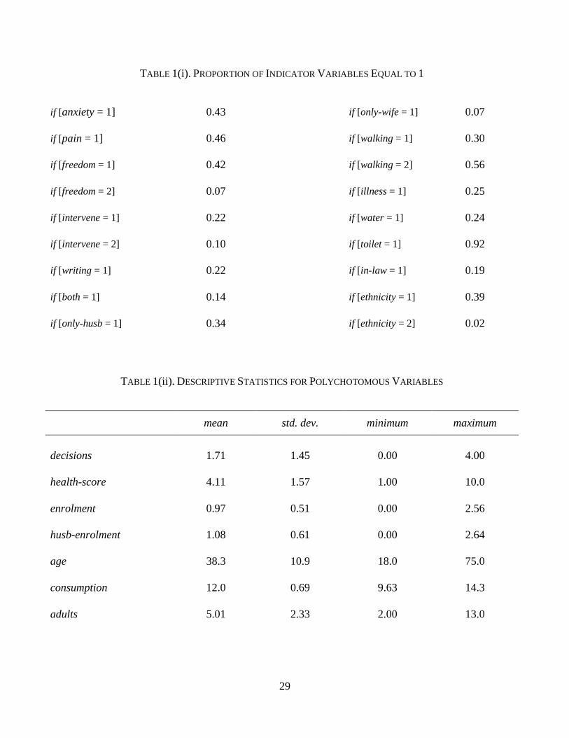
wellbeing of the married women in our sample, and to the determinants of their wellbeing.
(i) Subjective measures of wellbeing. All adults in the survey answered the following two questions
about their wellbeing: Do you feel anxious or depressed? Do you suffer from bodily pains? The possible
responses to these questions are: ‘often’ / ‘rarely’ / ‘never’. The proportion of women answering ‘never’
to these questions is only about 10%, so for each woman in our sample we construct two binary
variables as follows:
• Anxiety equals one if the response to the anxiety question is ‘often’, and equals zero otherwise.
• Pain equals one if the response to the physical pain question is ‘often’, and equals zero
otherwise.
5 Probably most of the absent husbands are working in the city.

8
A third question asks the respondents to rate their own general health on a 1-10 scale, with 10
representing the best health. We use the responses to this question as a third measure of subjective
wellbeing, but transform the data so that a score of 10 represents the poorest health: in this way, all three
measures are decreasing in the wellbeing of the respondent. The third measure is designated health-
score. These three measures capture women’s subjective perception of their mental and physical
wellbeing, which could depend on their level of empowerment through the amount of work they or their
children have to do, their consumption level, or the degree of mental and physical duress exerted by
their husband.6
The correlations between pain and the other two wellbeing indicators are quite high (ρ = 0.63 for
anxiety and ρ = 0.39 for health-score), but the correlation between anxiety and health-score is
somewhat lower (ρ = 0.20). The three different variables represent distinct but connected measures of a
woman’s subjective perception of her level of wellbeing.
(ii) Measures of women’s empowerment. The survey contains several different types of empowerment
measure, the first of which is based on the following question to women in the household: Can you go
out without the permission of your husband? The possible responses to this question are: ‘yes’ / ‘it
depends on the context’ / ‘no’. From these responses we construct a trivalent variable:
• Freedom equals two if the response is ‘yes’, equals one if the response is ‘it depends’, and
equals zero otherwise.
Secondly, the survey contains a series of questions about decisions within the home, based on those of
Allendorf (2007). Responses to four of these questions will be used in our model: Who makes decisions
6 Our three wellbeing variables represent a subset of the subjective measures of wellbeing used in larger questionnaires
such as the General Health Questionnaire and the Mental Health Inventory. See Das et al. (2008) for a discussion of
alternative survey measures in developing countries.

9
concerning your health? Who makes decisions concerning daily expenditures? Who makes decisions
concerning large expenditures? Who makes decisions concerning family visits? The alternative
responses to this question are: ‘me’ / ‘my husband’ / ‘someone else’. The correlations between the
responses to these questions are very high. If one constructs a set of binary variables equal to one if the
response is ‘me’ and equal to zero otherwise, the first principal component of the four variables (with
weights of 0.51, 0.52, 0.51 and 0.46) explains 56% of their overall variation. Therefore, we summarize
the four sets of responses by adding together the four binary variables. The resulting empowerment
measure, designated decisions, has a maximum value of four and a minimum value of zero.7
Thirdly, the survey contains the interviewer’s record of how the husband behaved while the wife
was being interviewed. In some cases the husband was not present at all, either because he was at home
but chose not to listen to the interview, or because he was happy for the wife to be interviewed while he
was out. In other cases the husband insisted on being present at the interview but remained passive.
Finally, there were some cases in which the husband verbally intervened in the interview. From this
information we construct a third empowerment variable:
• Intervene equals two if the husband intervened in the interview, equals one if he was present
but passive, and equals zero otherwise.
We take higher values of this variable to indicate that the husband is more inclined to monitor and
control his wife’s behavior. Conditional on freedom and decisions, an increase in intervene represents
less empowerment.8 However, although the correlation between freedom and decisions is quite high (ρ
7 The survey also includes questions about decisions concerning the woman’s children, but we do not use these,
because whether the woman has children may be endogenous to her subjective wellbeing. 8 It is also possible that the husband’s behavior affects the wife’s responses to the empowerment questions on which the
variables freedom and decisions are based. If this is this case, and if empowerment affects wellbeing, then we should
10
= 0.41), there is almost no correlation between intervene and freedom (ρ = 0.00) or intervene and
decisions (ρ = –0.01). One possible explanation for the lack of correlation is that that a low value of
intervene indicates a high level of mutual trust between husband and wife that is consistent either with
gender equality or with a reliably submissive wife. In this case, a high value of intervene indicates a lack
of trust and more potential for conflict within the home, and although there is no information about
domestic violence in the survey – this is too sensitive an issue – it is possible that intervene is positively
correlated with the incidence of violence.9
(iii) Other individual-specific covariates of wellbeing. Responses to other survey questions provide
information about the women’s age, education, physical health and ethnicity, characteristics that have
been found to affect subjective wellbeing in other developing countries (Das et al., 2008). Wellbeing
could also depend on whether the woman is married to the household head or some more junior male.10
The individual-specific covariates are as follows:
• Writing equals one if the woman can write a letter in French (which is the business language of
Senegal), and equals zero otherwise.
• Enrolment is equal to the log of the highest school grade for which the woman was ever
enrolled. (Using levels instead of logs makes very little difference to the final results.)
• Age is the woman’s age in years.
find that the interaction terms intervene × freedom and intervene × decisions are significant explanatory variables in
the wellbeing regressions. This turns out not to be the case. 9 The proportion of women in the sample for whom intervene > 0 is just over 30%, which is similar to the estimated
incidence of domestic violence in Senegal (Integrated Regional Information Networks, 2008). 10 There is also information about the seniority of each wife in the polygamous marriages, but adding a seniority
variable to the wellbeing regression does not produce a significant coefficient, and has no noticeable effect on the size
or significance levels of the other variables.
11
• Walking equals two if the woman can easily walk five kilometers, equals one if she can walk
this distance with difficulty, and equals zero if she cannot walk this distance.11
• Illness equals one if the woman suffers from a chronic illness, and equals zero otherwise.
• In-law equals one if the woman is married to a male relative of the household head, and equals
zero if she is married to the household head.
• Ethnicity equals two if the woman is neither Wolof nor Peul, equals one if she is Peul and
equals zero if she is Wolof.
(iv) Household-level covariates of wellbeing.
In addition to the individual responses, the survey contains information about household characteristics
provided by the household head. This allows us to measure the household’s size and its level of material
comfort, both of which have been found to affect individual wellbeing in other developing countries
(Das et al., 2008):
• Consumption is the log of the total annual value of household consumption per adult, measured
in CFA Francs.12
• Water equals one if the household has access to some improved water source (for example, a
well or borehole), and equals zero if the household relies on river water.
• Toilet equals one if the household has some type of toilet, and equals zero otherwise.
• Adults equals the number of adults in the household.
11 There are other measures of physical capacity in the survey, but these are highly correlated with walking, and have
no additional explanatory power in the wellbeing regressions. 12 Survey responses also indicate the share of household expenditure controlled by the woman, but this share is highly
correlated with the empowerment variables, and has no additional explanatory power in the wellbeing regressions.

12
There are three versions of our wellbeing model, one for each of the alternative wellbeing measures. In
each model, the set of explanatory variables comprises the continuous variables listed above –
enrolment, age, consumption and adults (decisions is also treated as a continuous variable) – plus a set
of indicator variables for all of the other individual and household characteristics – for example,
if [freedom = 2], if [freedom = 1] and if [water = 1]. Some of the 668 married and cohabiting women
failed to respond to some of the survey questions, so our final sample comprises 627 women in the
anxiety model, and 628 women in the other two models. Sample statistics for all of the variables appear
in Table 1. (The table also includes some variables to be used as instruments for women’s
empowerment; these will be discussed later.) It can be seen that the women in the sample are roughly
evenly split between those who are often anxious or depressed (anxiety = 1) and those who are not,
between those who often experience bodily pain (pain = 1) and those who are not, and between those
who have some freedom to leave the home (freedom > 0) and those who do not. The standard deviations
of the variables health-score and decisions are over half as large as their mean values. In this sense,
there is substantial variation in both subjective wellbeing and empowerment. The next section presents
the model used to explore how wellbeing and empowerment are connected.
[Table 1 here]
4. The Model
4.1 Results assuming the exogeneity of women’s empowerment and sample selection
Because the data have a nested structure (individuals within marital units within households within
villages), it is possible to model wellbeing using mixed-effects models, with parameters that capture the
variance in the unobserved heterogeneity at each level of aggregation. However, it turns out that when
such models are applied to our data, the estimated variances at the marital unit and village level are

13
insignificantly different from zero. Therefore, the results we discuss here are based on simple random-
effects models of individuals within households.
We begin by discussing the results of models which assume that the empowerment variables and
selection into the sample of married and cohabiting women are exogenous, and which are summarized in
Table 2. For the binary wellbeing measures anxiety and pain we fit a random-effects probit model:
( ) ( ) ( )2P 1 , , ~ N ,i j jk ikkanxiety x i j ε εβ ε ε µ σ= = Φ ⋅ + ∈∑ (1)
( ) ( ) ( )2P 1 , , ~ N ,i j jk ikkpain x i j η ηγ η η µ σ= = Φ ⋅ + ∈∑ (2)
For the health-score measure we fit a random-effects tobit model:
( ) ( )2 2, , ~ N , , ~ N 0,i j i j ik ikky x i j ϕθ θδ θ ϕ θ µ σ ϕ σ= ⋅ + + ∈∑ (3)
( )( )max 1, min 10,i ihealth score y=
Here, Φ(.) is the cumulative normal density function, the β, γ and θ terms are parameters to be
estimated, xik is the value of the k
th explanatory variable for the i
th woman, and ε j, η j and θ j are random
effects pertaining to the jth household. (Although the random effects all have variances significantly
greater than zero, the results from pooled probit and tobit models are very similar; see Appendix Table
A1.) In Table 2, the A column in the anxiety panel includes the estimated values of the β parameters in
equation (1), the A column in the pain panel includes the estimated values of the γ parameters in
equation (2), and the A column in health-score panel includes the estimated values of the δ parameters
in equation (3). The relevant t-ratios are also reported, along with the marginal effects (dP / dx) implicit in
the β and γ estimates, evaluated at the mean values of P.
There is some similarity in the estimated effects of the empowerment variables across the three
wellbeing measures. First of all, freedom and intervene are significant determinants of wellbeing, but

14
decisions is not. Because of the high correlation between freedom and decisions, the t-ratio on the
decisions coefficient could be biased downwards. For this reason, Table 2 also includes versions of each
model in which either freedom or decisions is excluded: see columns B and C in each panel. It turns out
that the exclusion of one variable does not make any substantial difference to the coefficient and t-ratio
on the other, except in the health-score model, as discussed below.
The negative coefficients on if [freedom = 1] and if [freedom = 2] indicate that more freedom is
better for wellbeing. The transition from freedom = 0 to freedom = 1 (giving the woman some say in
whether she leaves the home) reduces the probability of her often feeling anxious or depressed by about
20 percentage points. The effect on the probability of often having bodily pains is very similar, and the
effect on the health score is to improve it by just over half a point (in other words, by one third of the
standard deviation of this variable). The transition from freedom = 0 to freedom = 2 (giving the woman
complete autonomy) has no significant effect in the anxiety model, which is an anomalous result, but
bear in mind that only 7% of women in the sample have complete autonomy. The transition to freedom
= 2 does have a significant effect in the other two models, reducing the probability of often having
bodily pains by over 30 percentage points and improving the health score by over half a point. The only
case in which there is a significant coefficient on decisions is in the health-score model with freedom
excluded: in this case, a unit rise in decisions is estimated to improve the health score by about 0.15
points. Overall, these results suggest that whether the woman is free to choose what to do with her time
– and in particular whether she has some say in whether she can go out when she wants to – is a key
determinant of her subjective wellbeing.
Table 2 also shows that intervene is a significant determinant of all measures of wellbeing. As
noted above, this variable represents a dimension of women’s empowerment that is quite distinct from
freedom and decisions. The positive coefficients on if [intervene = 1] in the anxiety and pain models

15
indicate that women with husbands present at their interview have lower levels of wellbeing, on average:
the probability of often feeling anxious or depressed is about 20 percentage points higher, and the
probability of often feeling bodily pain is about 15 percentage points higher. (There is no significant
effect in the health-score model.) The if [intervene = 2] coefficients are larger still, indicating that
women with husbands who intervene during the interview have especially low levels of wellbeing, on
average: the probability of often feeling anxious or depressed is about 40 percentage points higher, as is
the probability of often feeling bodily pain. These women’s health score is also significantly worse: on
average, the health-score variable is about half a point higher.
Of the other variables in the model, the ones with a significant and consistent effect across all
three measures of wellbeing are those capturing the woman’s age and physical condition. For every year
of age, the probability of feeling anxious or depressed and the probability of feeling bodily pains both
increase by about one percentage point; the health score worsens by about 0.025 points.13 Similarly,
having a chronic illness adds about 20-30 percentage points to the probability that a woman will often
feel anxious or depressed or feel bodily pains, and worsens her subjective health score by about one
point. The effects of not being able to walk five kilometers (compared with being able to walk this
distance easily) are about the same. In other words, the effect on the wellbeing variables anxiety and
pain of having a poor value of either freedom or intervene is similar in size to the effect of contracting a
chronic illness, or becoming severely physically incapacitated, or aging by several decades. (For the
health-score variable, the effects of freedom and intervene are slightly smaller in relative terms.)
Two other variables with a significant effect are enrolment (but only in the anxiety model) and
consumption (but only in the health-score model). Combining the marginal effects in Table 2 with the
13 Adding a quadratic term in age to the model produces a coefficient that is insignificantly different from zero. The
effect of age is monotonic and approximately linear: people in a country as poor as Senegal do not have any reason to
look forward to old age.

16
standard deviations in Table 1, a two standard deviation increase in the school enrolment variable
(∆enrolment = 1.0) reduces the probability of feeling anxiety or depression by about 15 percentage
points, and a two standard deviation increase in household consumption (∆consumption = 1.4) improves
the health score by about three quarters of a point. In this sense, in the subset of cases in which the
effects of education and consumption are statistically significant, their effects on wellbeing are of a
magnitude similar to those of age, physical condition and empowerment. However, the estimated effects
of education and consumption are not robust across all measures of wellbeing.
[Table 2 here]
4.2 Dealing with potential endogeneity and sample selection bias
It is possible that both the level of empowerment and selection into the sample of married and
cohabiting women are endogenous to wellbeing.14 In order to test for endogeneity, we first need to
model empowerment and selection as a function of some set of instruments.
For empowerment – as captured by freedom and intervene – the extra instruments used to
identify the model are measures of the husband’s level of education. Here, the exclusion restriction is
that conditional on the individual and household characteristics in lists (iii-iv) above, the husband’s
education affects his wife’s wellbeing only through the effect it has on her level of empowerment. Given
the wife’s education level, more education for the husband might increase empowerment (by socializing 14 It is also possible that consumption is endogenous, because consumption depends on income, income depends on the
wife’s labor productivity, and productivity depends on wellbeing. We also have an instrument for consumption:
whether the water supply for the household’s farm was affected by salt contamination in the last year. (Salt dissolves
into water channels from the surrounding rock, but the local geology is so variable that it is impossible to predict when
this will happen, so salt contamination is a genuinely random shock.) Salt contamination is a strong instrument with a
significant effect on consumption (p < 0.01). We test for the endogeneity of consumption using this instrument, and
find that it is not possible to reject the null hypothesis that consumption is exogenous to wellbeing. Further details are
available on request.

17
the husband so that he has a preference for gender equality) or reduce it (by increasing his bargaining
ability). We use survey data on the husband’s highest level of school enrolment (designated husb-
enrolment) and also interact male and female literacy by constructing the following variables:
• Both equals one if both the husband and wife can write a letter in French, and equals zero
otherwise.
• Only-husb equals one if only the husband can write a letter in French, and equals zero
otherwise.
• Only-wife equals one if only the wife can write a letter in French, and equals zero otherwise.
Descriptive statistics for these four education variables appear in Table 1. We fit random-effects ordered
probit models for freedom and intervene as a function of the four education variables plus the other
regressors in lists (iii-iv), but omitting writing, which is now superfluous. The regression equations are
as follows:
( ) ( ) ( )2
1P 0 1 , , ~ N ,i j jk ikkfreedom z i j υ υζ υ κ υ µ σ= = −Φ ⋅ + − ∈∑ (4)
( ) ( ) ( )1 2P 1i j jk ik k ikk kfreedom z zζ υ κ ζ υ κ= = Φ ⋅ + − −Φ ⋅ + −∑ ∑
( ) ( )2P 2i jk ikkfreedom zζ υ κ= = Φ ⋅ + −∑
( ) ( ) ( )2
1P 0 1 , , ~ N ,i j jk ikkintervene z i j ω ωξ ω λ ω µ σ= = −Φ ⋅ + − ∈∑ (5)
( ) ( ) ( )1 2P 1i j jk ik k ikk kintervene z zξ ω λ ξ ω λ= = Φ ⋅ + − −Φ ⋅ + −∑ ∑
( ) ( )2P 2i jk ikkintervene zξ ω λ= = Φ ⋅ + −∑
Here, zik designates the value of the kth instrument for individual i, υ j and ω j are household-level random
effects, and the ζ, ξ, κ and λ terms represent parameters to be estimated. These models are similar to the

18
ones in Allendorf (2007) and Anderson and Eswaran (2009) discussed above, but with a larger set of
explanatory variables.
Table 3 presents estimates of the ζ and ξ parameters in equations (4-5), along with the
corresponding marginal effects for the transition from zero to one (‘m.e. 1’) and from one to two (‘m.e.
2’). It can be seen that both and only-husb are significant determinants of freedom, while both is a
significant determinant of intervene. The estimates suggest that freedom is higher when the husband is
literate in French, regardless of whether the wife is literate, but that intervene is lower only when both
the husband and wife are literate in French. Nevertheless, the signs of these effects all imply that male
literacy is beneficial for women’s empowerment, as measured by a higher value of freedom or a lower
value of intervene. In contrast to these effects, women whose husbands have a higher level of school
enrolment experience a lower level of freedom, on average. One interpretation of this apparent
contradiction is that (i) fluency is French is associated with the adoption of ‘modern’ values, including
gender equality, but (ii) conditional on this effect, more education, which raises husbands’ bargaining
power within the home, tends to reduce women’s empowerment.
Table 3 suggests three other noteworthy determinants of empowerment. Firstly, the negative and
significant coefficient on the in-law variable in the intervene equation indicates that the household head
is less likely to intervene in the interview of a woman who is not his wife. In this sense, marriage to a
more senior man is associated with less empowerment, on average. Secondly, the negative and
significant coefficient on adults in the freedom equation and the positive and significant coefficient in
the intervene equation indicates that women in smaller households are more empowered. Thirdly, there
is negative and significant coefficient on consumption in the freedom equation and a positive and
significant coefficient in the intervene equation. This indicates that on average, and controlling for other
factors, women in households with a higher per capita consumption have less empowerment, perhaps

19
because poverty is associated with lower male bargaining power. This result is consistent with the
sentiments of the Wolof women interviewed by Perry (2005):
‘Although her husband is the richest man in the village, Ndey proclaimed that she would rather be in her
sister’s marriage to a poor farmer than in her own to a rich man. Another woman observed, “Those
without money [are] the ones who take best care of their wives.”’
One characteristic of the random-effects estimates in Table 3 is that marginal effects for the
second transition are insignificantly different from zero, which implies that the husband’s education is
not a strong instrument for if [freedom = 2] or if [intervene = 2]. (These are the most infrequent
outcomes, representing less than 10% of the sample in each case.) The insignificance of these marginal
effects arises from very imprecise random-effects estimates of the transition parameters κ2 and λ2, which
is perhaps not surprising when there is such a small number of observations of freedom = 2 and
intervene = 2, and an even smaller number of households where these values are observed. The estimate
of the transition parameters becomes more precise if we set the variances of the random effects to zero
and fit pooled ordered probit models, so pooled probit estimates are also shown in Table 3. Comparing
the two sets of estimates, the ζ and ξ parameters are quite similar but the pooled probit marginal effects
for the second transition are much larger and significantly different from zero. For this reason, we will
consider two alternative forms of the empowerment variable endogeneity tests, one based on the
random-effects estimates and one on the pooled estimates.
[Table 3 here]
It is also necessary to model selection into the sample of married and cohabiting women. Here,
the model is identified by noting that the youngest and oldest women in the survey are much less likely
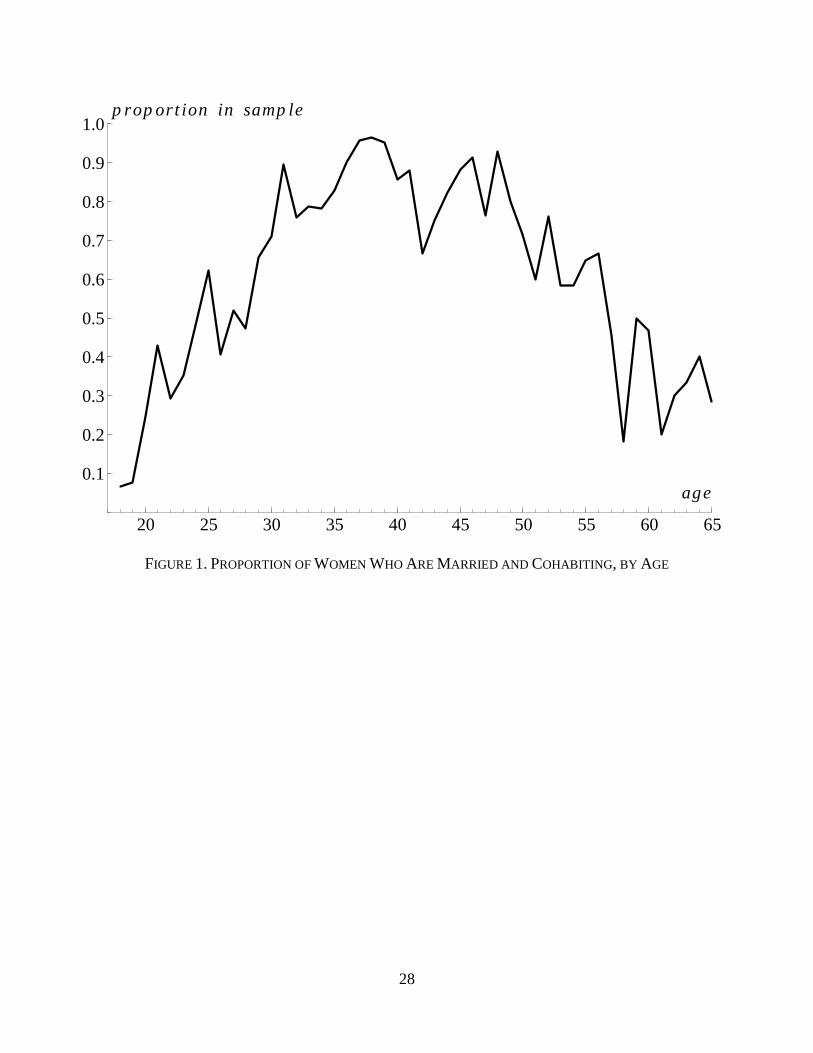
to be married, as shown in Figure 1. Some women are not married until their late twenties, and some are

20
already widowed by their early fifties. In order to model the probability of being in the married and
cohabiting sample, we first define the variable range as follows:15
• range = [age – 50] if age > 50
= [30 – age] if age < 30
= 0 otherwise.
Next we define an indicator variable for selection into the married and cohabiting sample:
• marco equals one if the woman is in the sample, and equals zero otherwise.
These two variables are constructed for the 1,060 women in the sample for whom observations of the
variables in lists (iii-iv) above are also available.16 We then fit the following random-effects probit
model to the data:
( ) ( ) ( )/ 2P 1 , , ~ N ,i j jk ikkmarco z i j ϖ ϖα ϖ ϖ µ σ= = Φ ⋅ + ∈∑ (6)
Here, /
ikz designates the value of the kth instrument for individual i (the instrument set incorporating
range plus all the variables in lists (iii-iv) except in-law, which is not defined for unmarried women) and
ϖ j is a household-level random effect.
Table 4 shows the estimates of the α parameters, along with the corresponding estimates from a
pooled probit model, which are very similar. The table shows that the three statistically significant
determinants of the sample selection are range, age and consumption. As anticipated, the youngest and
15 Using range to identify the sample selection relies on the assumption that the direct effect of age on wellbeing is
monotonic. Our observations in footnote 13 provide support for this assumption. 16 Of these 1,060 women, 642 are married and cohabiting: the 628 who make up the main sample plus 14 others for
whom observations of the subjective wellbeing or empowerment variables are not available.
21
oldest women are significantly less likely to be married and cohabiting. Also, women who are married
and cohabiting are more likely to be found in richer households.
[Figure 1 and Table 4 here]
Having modeled the empowerment variables and sample selection, it is possible to test whether
they are endogenous to women’s wellbeing. In order to do this, we use the models in Tables 3-4 to
construct estimates of the following Inverse Mills Ratios (IMRs):
• ( ) ( )= dP 1 P 1i i imarco marcoπ = = is the IMR for selection into the sample.
• ( ) ( )= dP Pni i ifreedom n freedom nτ ≥ ≥ , n ∈ {1,2}, is the IMR for each positive value of
freedom.
• ( ) ( )= dP Pni i iintervene i intervene iψ ≥ ≥ , n ∈ {1,2}, is the IMR for each positive value of
intervene.
Two sets of IMRs are constructed, one using the random-effects estimates in Tables 3-4 and the other
using the pooled estimates. We test for sample selection bias by adding the estimated values of iπ to
equations (1-3). Similarly, we test for the endogeneity of freedom by adding the estimated values of 1iτ
and 2iτ to equations (1-3), and for the endogeneity of intervene by adding the estimated values of 1
iψ
and 2iψ to equations (1-3). In each case, the null hypothesis is that there is no endogeneity bias. This
null is tested against the alternative using a Likelihood Ratio test for the significance of the IMR terms.
Table 5 reports two sets of p-values corresponding to these test statistics, one for the IMRs from the
random-effects estimates of equations (4-6), and one for the IMRs from the pooled estimates. Table 5
shows that the iπ and niτ terms are never statistically significant, so the null hypotheses that the sample

22
selection and the value of freedom are exogenous to wellbeing cannot be rejected. However, the niψ
terms based on the pooled estimates of equation (5) are significant in the pain and health-score models,
so there is evidence that intervene is endogenous to these two measures of wellbeing.
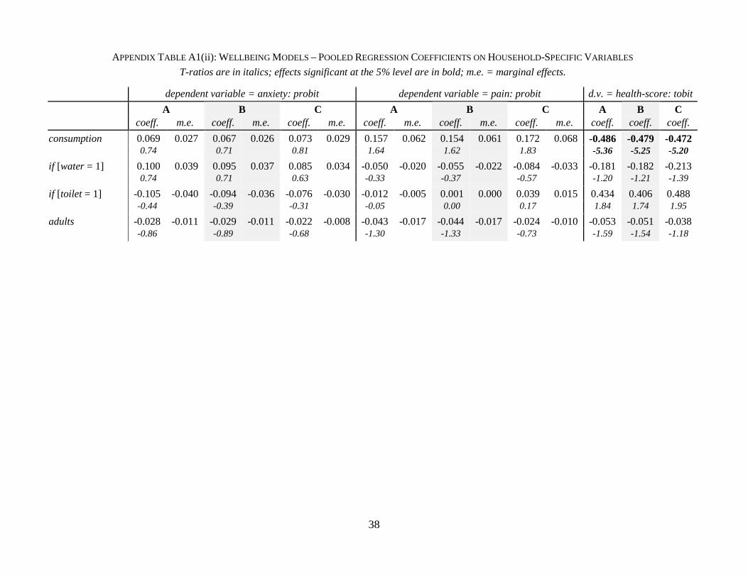
In light of the likely endogeneity of intervene to pain and health-score, Table 6 reports
parameter values from an augmented version of equations (2-3) that includes the pooled estimates of
1iψ and 2
iψ as additional explanatory variables in order to correct for the endogeneity bias. The
accompanying t-ratios are computed using a bootstrap with 1,000 replications. The figures in Table 6
correspond to those in the B columns of Table 2 (the model excluding decisions).17 In Table 6, the
estimated effects of freedom and intervene on pain are slightly smaller than in Table 2, but still
statistically significant. Estimates of the other parameters in the pain model are very similar, except that
the age effect is smaller and no longer statistically significant. There is very little difference between
Table 2 and Table 6 in the values of the parameters in the health-score model. In this sense, correcting
for endogeneity makes little difference to our conclusions.
[Tables 5-6 here]
5. Discussion
Analysis of survey data from rural Senegal indicates that the effects of women’s empowerment on their
wellbeing – as measured by subjective indicators of psychological and physical health – are large.
Differences in the level of empowerment matter as much as (or more than) differences in consumption,
education and morbidity. This brings into question the relatively small effort that international donors
17 The Table 6 estimates of the parameters in the pain model are based on a pooled probit regression. It was not
possible to compute reliable t-ratios for the random-effects version of the model, because in many of the bootstrap
replications the log-likelihood function was very flat (and much flatter than with the actual data), so the bootstrap
parameter estimates were highly variable.

23
put into women’s empowerment initiatives, compared with more traditional development goals. One
possible justification of the focus on the traditional development goals is that improvements in other
areas will lead to more women’s empowerment in the long run, as suggested by the cross-country
macroeconomic data. However, our micro-econometric analysis does not provide strong evidence for
such effects. Firstly, the effect of education on women’s empowerment is ambiguous. Some education
outcomes such as male literacy are associated with more empowerment, which suggests that educating
boys can improve their attitudes towards women. However, for a given literacy level more male
education reduces women’s empowerment, possibly because it raises men’s bargaining power within the
home. Secondly, women in poor households have more empowerment, ceteris paribus. This may again
reflect a positive correlation between the overall level of development of the household and the
bargaining power of its (male) head, to the detriment of rich men’s wives.
There is a contradiction here between the cross-country macroeconomic evidence and our micro-
econometric results. Understanding the reasons for this contradiction is work for the future, and the
analysis of Senegalese data discussed in this paper has yet to be replicated for other parts of the
developing world, so it is still not clear how widely applicable our results are. Nevertheless, our results
shed doubt on whether general development initiatives within an individual country will improve the lot
of its women, and there is reason to be concerned about the lack of attention currently given to women’s
empowerment by aid donors. In the absence of aid programs that specifically target empowerment, it is
quite possible that development initiatives which are successful according to standard metrics (such as
per capita consumption or education levels) will worsen the lives of half of the target population.
24
References
Allendorf, K. (2007) ‘Do women’s land rights promote empowerment and child health in Nepal?’ World
Development 35 (11): 1975-88.
Allendorf, K. (2010) ‘The quality of family relationships and use of maternal health-care services in
India,’ Studies in Family Planning 41(4): 263-276.
Anderson, S. and Eswaran, M. (2009) ‘What determines female autonomy? Evidence from Bangladesh,’
Journal of Development Economics 90: 179-191.
Ashraf, N. (2009) “Spousal control and intra-household decision making: an experimental study in the
Philippines,” American Economic Review 99(4): 1245-77.
Behrman, J.R., and Hoddinott, J. (2005) ‘Programme evaluation with unobserved heterogeneity and
selective implementation: the Mexican PROGRESA impact on child nutrition,” Oxford Bulletin of
Economics and Statistics 67(4): 547-69.
Bobonis, G.J. (2009) ‘Is the allocation of resources within the household efficient? New evidence from a
randomized experiment,’ Journal of Political Economy 117(3): 453-503.
Brown, P.H. (2003) ‘Dowry and intrahousehold bargaining: evidence from China,’ William Davidson
Institute Working Paper 2003-608. William Davidson Institute, University of Michigan, Ann Arbor, MI.
Das, J., Do, Q-T., Friedman, J. and McKenzie, D. (2008) ‘Mental health patterns and consequences:
results from survey data in five developing countries,’ World Bank Economic Review 23(1): 31-55.
Deininger, K., Goyal, A. Nagarajan, H. (2010) ‘Inheritance law reform and women’s access to capital:
evidence from India’s Hindu Succession Act, No 5338,’ Policy Research Working Paper, World Bank,
Washington, DC.
Doepke, M., Tertilt, M. and Voena, A. (2012) ‘The economics and politics of women’s rights,’ Annual
Review of Economics 4: 339-72.
25
Doss, C.R. (2001) ‘Is risk fully pooled within the household? Evidence from Ghana.” Economic
Development and Cultural Change 50(1): 101-30.
Doss, C.R. (2013) ‘Intrahousehold bargaining and resource allocation in developing countries,’ World
Bank Research Observer 28: 52-78.
Duflo, E. (2003) ‘Grandmothers and granddaughters: old-age pensions and intra-household allocation in
South Africa,’ World Bank Economic Review 17(1): 1-25.
Duflo, E. and Udry, C. (2004) ‘Intra-household resource allocation in Côte d’Ivoire: social norms,
separate accounts and consumption choices.” NBER Working Paper 10498, National Bureau of
Economic Research, Cambridge, MA.
Dunkle, K.L., Jewkes, R.K., Brown, H.C., Gray, G.E., McIntryre, J.A. and Harlow, S.D. (2004)
‘Gender-based violence, relationship power, and risk of HIV infection in women attending antenatal
clinics in South Africa,’ The Lancet 363: 1415-1421.
Durevall, D. and Lindskog, A. (2013) ‘Intimate Partner Violence and HIV in sub-Saharan Africa,’
Working Paper, Department of Economics and Gothenburg Centre of Globalization and Development,
University of Gothenburg, Gothenburg, Sweden.
Furuta, M. and Salway, S. (2006) ‘Women’s position within the household as a determinant of maternal
health care use in Nepal,’ International Family Planning Perspectives 32(1): 17-27.
Golding, J. (1999) ‘Intimate partner violence as a risk factor for mental disorders: a meta-analysis,’
Journal of Family Violence 14(2): 99-132.
Integrated Regional Information Networks (2008) ‘Senegal: beaten in silence,’ www.irinnews.org/
Report/ 78743/SENEGAL-Beaten-in-silence.
26
Iversen, V., Jackson, C., Kebede, B., Munro, A. and Verschoor, A. (2006) ‘What’s love got to do with
it? An experimental test of household models in East Uganda,’ Working Paper 2006-01, Centre for the
Study of African Economies, Oxford, UK.
Hidrobo, M. and Fernald, L. (2013) ‘Cash transfers and domestic violence,’ Journal of Health
Economics 32: 304-319.
Lim, S.S., Dandona, L., Hoisington, J.A., James, S.L., Hogan, M.C. and Gakidou, E. (2010) ‘India’s
Janani Suraksha Yojana, a conditional cash transfer programme to increase births in health facilities: an
impact evaluation.” The Lancet 375: 2009-2023.
Lépine, A. (2009) ‘Data collection,’ mimeo, Department of Global Health and Development, London
School of Tropical Medicine and Hygiene, London, UK.
Lépine, A. (2012) ‘Three essays in health microeconomics in developing countries: evidence from rural
Senegal,’ Ph.D. dissertation, University of Otago, Dunedin, New Zealand.
Lépine, A. and Le Nestour, A. (2013) ‘The determinants of health care utilisation in rural Senegal,’
Journal of African Economies 22(1): 163-186.
Maluccio, J. and Flores, R. (2005) ‘Impact evaluation of a conditional cash transfer program: the
Nicaraguan Red de Protección Social,’ Research Report 141, International Food Policy Research
Insititute, Washinton, DC.
Miner, S., Ferrer, L., Cianelli, R., Bernales, M. and Cabieses, B. (2011) ‘Intimate partner violence and
HIV risk behaviors among socially disadvantaged Chilean women,’ Violence Against Women 17(4):
517-531.
Mistry, R., Galal, O. and Lu, M. (2009) ‘Women’s autonomy and pregnancy care in rural India: a
contextual analysis,’ Social Science and Medicine 69: 926-933.
27
Perry, D.L. (2005) ‘Wolof women, economic liberalization, and the crisis of masculinity in rural
Senegal,’ Ethnology 44(3): 207-226.
Qian, N. (2008) ‘Missing women and the price of tea in China: The effect of sex-specific earnings on
sex imbalance,’ Quarterly Journal of Economics 123(3): 1251-85.
Rangel, M.A. (2006) ‘Alimony Rights and Intrahousehold Allocation of Resources: Evidence from
Brazil,’ Economic Journal 116(513): 627-58.
Sen, A. (1991) ‘Welfare, preference and freedom,’ Journal of Econometrics 50: 15-29.
United Nations (2013) ‘Goal 3: promote gender equality and empower women,’ www.un.org/
millenniumgoals/gender.shtml.
28
20 25 30 35 40 45 50 55 60 65
0.1
0.2
0.3
0.4
0.5
0.6
0.7
0.8
0.9
1.0
age
p rop ort ion in samp le
FIGURE 1. PROPORTION OF WOMEN WHO ARE MARRIED AND COHABITING, BY AGE
29
TABLE 1(i). PROPORTION OF INDICATOR VARIABLES EQUAL TO 1
if [anxiety = 1] 0.43 if [only-wife = 1] 0.07
if [pain = 1] 0.46 if [walking = 1] 0.30
if [freedom = 1] 0.42 if [walking = 2] 0.56
if [freedom = 2] 0.07 if [illness = 1] 0.25
if [intervene = 1] 0.22 if [water = 1] 0.24
if [intervene = 2] 0.10 if [toilet = 1] 0.92
if [writing = 1] 0.22 if [in-law = 1] 0.19
if [both = 1] 0.14 if [ethnicity = 1] 0.39
if [only-husb = 1] 0.34 if [ethnicity = 2] 0.02
TABLE 1(ii). DESCRIPTIVE STATISTICS FOR POLYCHOTOMOUS VARIABLES
mean std. dev. minimum maximum
decisions 1.71 1.45 0.00 4.00
health-score 4.11 1.57 1.00 10.0
enrolment 0.97 0.51 0.00 2.56
husb-enrolment 1.08 0.61 0.00 2.64
age 38.3 10.9 18.0 75.0
consumption 12.0 0.69 9.63 14.3
adults 5.01 2.33 2.00 13.0

30
TABLE 2(i): WELLBEING MODELS – RANDOM-EFFECTS REGRESSION COEFFICIENTS ON INDIVIDUAL-SPECIFIC VARIABLES T-ratios are in italics; effects significant at the 5% level are in bold; m.e. = marginal effects.
dependent variable = anxiety: probit dependent variable = pain: probit d.v. = health-score: tobit
A B C A B C A B C coeff. m.e. coeff. m.e. coeff. m.e. coeff. m.e. coeff. m.e. coeff. m.e. coeff. coeff. coeff.
if [freedom = 1] -0.627 -0.201 -0.604 -0.196
-0.677 -0.237 -0.670 -0.235
-0.526 -0.619
-2.87 -3.01 -3.48 -3.69 -3.67 -4.72
if [freedom = 2] -0.150 -0.055 -0.108 -0.040
-1.061 -0.328 -1.035 -0.323
-0.532 -0.620
-0.43 -0.32 -3.19 -3.17 -2.25 -2.70
decisions 0.018 0.007
-0.059 -0.022 0.007 0.003
-0.092 -0.036 -0.073
-0.145
0.26 -0.93 0.12 -1.65 -1.60 -3.44
if [intervene = 1] 0.500 0.197 0.498 0.196 0.551 0.217 0.384 0.152 0.385 0.153 0.407 0.161 -0.147 -0.137 -0.119
2.33 2.32 2.52 1.97 1.96 2.08 -1.010 -0.94 -0.82
if [intervene = 2] 1.048 0.393 1.050 0.393 1.013 0.382 1.057 0.377 1.063 0.378 0.986 0.357 0.510 0.515 0.480
3.38 3.37 3.21 3.75 3.74 3.49 2.48 2.51 2.31
if [writing = 1] 0.370 0.145 0.368 0.144 0.406 0.159 0.037 0.015 0.036 0.014 -0.015 -0.006 0.138 0.140 0.129
1.31 1.30 1.44 0.15 0.14 -0.06 0.73 0.74 0.68
enrolment -0.464 -0.157 -0.466 -0.158 -0.504 -0.168 -0.040 -0.016 -0.043 -0.017 -0.080 -0.031 -0.256 -0.255 -0.289
-2.04 -2.05 -2.20 -0.19 -0.21 -0.39 -1.70 -1.69 -1.91
age 0.020 0.008 0.021 0.008 0.021 0.008 0.030 0.012 0.030 0.012 0.030 0.012 0.025 0.023 0.025
2.20 2.29 2.25 3.46 3.55 3.44 4.06 3.86 4.11
if [walking = 1] -0.542 -0.179 -0.559 -0.184 -0.514 -0.171 -0.247 -0.095 -0.266 -0.102 -0.215 -0.083 -0.380 -0.400 -0.361
-2.02 -2.09 -1.90 -1.05 -1.12 -0.91 -2.14 -2.27 -2.02
if [walking = 2] -0.852 -0.252 -0.869 -0.256 -0.834 -0.248 -1.174 -0.348 -1.197 -0.353 -1.139 -0.343 -1.061 -1.078 -1.044
-3.20 -3.26 -3.10 -4.78 -4.86 -4.64 -6.25 -6.38 -6.10
if [illness = 1] 0.701 0.274 0.698 0.273 0.693 0.271 0.595 0.231 0.593 0.231 0.563 0.220 0.925 0.928 0.908
3.56 3.53 3.49 3.32 3.29 3.14 7.05 7.06 6.86
if [in-law = 1] -0.389 -0.135 -0.375 -0.131 -0.354 -0.123 0.088 0.035 0.105 0.042 0.088 0.035 -0.134 -0.126 -0.104
-1.53 -1.48 -1.38 0.39 0.47 0.39 -0.80 -0.76 -0.62
if [ethnicity = 1] 0.257 0.100 0.268 0.105 0.424 0.167 0.087 0.035 0.098 0.039 0.296 0.118 0.263 0.248 0.412
1.24 1.29 2.04 0.48 0.54 1.64 1.88 1.78 3.02
if [ethnicity = 2] -1.094 -0.294 -1.089 -0.293 -1.086 -0.292 -0.105 -0.041 -0.099 -0.039 -0.016 -0.006 -1.598 -1.635 -1.552
-1.62 -1.60 -1.56 -0.20 -0.19 -0.03 -3.72 -3.81 -3.56

31
TABLE 2(ii): WELLBEING MODELS – RANDOM-EFFECTS REGRESSION COEFFICIENTS ON HOUSEHOLD-SPECIFIC VARIABLES T-ratios are in italics; effects significant at the 5% level are in bold; m.e. = marginal effects.
dependent variable = anxiety: probit dependent variable = pain: probit d.v. = health-score: tobit
A B C A B C A B C coeff. m.e. coeff. m.e. coeff. m.e. coeff. m.e. coeff. m.e. coeff. m.e. coeff. coeff. coeff.
consumption 0.109 0.042 0.107 0.041 0.127 0.049 0.197 0.078 0.197 0.078 0.232 0.092 -0.506 -0.496 -0.488 0.78 0.76 0.88 1.59 1.57 1.83 -5.30 -5.19 -5.03
if [water = 1] 0.126 0.048 0.123 0.048 0.102 0.039 -0.060 -0.024 -0.065 -0.025 -0.104 -0.041 -0.136 -0.138 -0.166 0.58 0.57 0.46 -0.32 -0.34 -0.54 -0.93 -0.94 -1.11
if [toilet = 1] -0.248 -0.089 -0.235 -0.085 -0.218 -0.079 -0.064 -0.025 -0.055 -0.022 -0.009 -0.003 0.369 0.335 0.404 -0.71 -0.67 -0.61 -0.21 -0.18 -0.03 1.57 1.43 1.69
adults -0.026 -0.010 -0.027 -0.010 -0.015 -0.005 -0.054 -0.021 -0.056 -0.022 -0.030 -0.012 -0.060 -0.057 -0.046 -0.55 -0.58 -0.31 -1.31 -1.33 -0.73 -1.88 -1.80 -1.44
random effect σ 1.165 1.175 1.215 0.915 0.932 0.961 0.801 0.802 0.835 4.83 4.86 4.91 4.35 4.42 4.50 9.22 9.20 9.70

32
TABLE 3(i): EMPOWERMENT MODELS – ORDERED PROBIT REGRESSION COEFFICIENTS ON INDIVIDUAL-SPECIFIC VARIABLES T-ratios are in italics; effects significant at the 5% level are in bold; m.e. = marginal effects.
dependent variable = freedom dependent variable = intervene pooled regression random effects regression pooled regression random effects regression coeff. m.e.1 m.e.2 coeff. m.e.1 m.e.2 coeff. m.e.1 m.e.2 coeff. m.e.1 m.e.2 if [both = 1] 0.596 0.226 0.105 0.887 0.330 0.009 -0.579 -0.162 -0.052 -1.138 -0.094 -0.000 2.59 2.46 -2.08 -2.10 if [only-husb = 1] 0.405 0.158 0.062 0.691 0.266 0.005 -0.079 -0.027 -0.010 0.154 0.030 0.000 2.90 2.77 -0.51 0.41 if [only-wife = 1] 0.254 0.100 0.035 0.754 0.287 0.006 0.002 0.001 0.000 -0.274 -0.041 -0.000 1.12 1.90 0.01 -0.49 husb-enrolment -0.346 -0.135 -0.030 -0.659 -0.230 -0.001 -0.034 -0.012 -0.005 -0.247 -0.037 -0.000 -3.09 -3.36 -0.27 -0.85 enrolment 0.194 0.077 0.026 0.296 0.118 0.001 0.108 0.038 0.016 0.426 0.098 0.001 1.40 1.34 0.68 1.27 age 0.004 0.002 0.000 0.014 0.005 0.000 0.008 0.003 0.001 0.010 0.002 0.000 0.68 1.40 1.32 0.75 if [walking = 1] -0.024 -0.009 -0.003 0.063 0.025 0.000 0.151 0.054 0.023 -0.007 -0.001 -0.000 -0.13
0.22
0.86
-0.02
if [walking = 2] -0.005 -0.002 -0.001 0.036 0.014 0.000 0.348 0.129 0.062 0.332 0.072 0.000 -0.03 0.13 2.09 0.79 if [illness = 1] 0.083 0.033 0.010 0.269 0.107 0.001 -0.135 -0.045 -0.017 -0.072 -0.012 -0.000 0.72 1.28 -1.15 -0.27 if [in-law = 1] -0.098 -0.039 -0.010 -0.083 -0.033 -0.000 -0.823 -0.207 -0.062 -1.829 -0.101 -0.000 -0.60 -0.33 -4.59 -4.04 if [ethnicity = 1] -0.727 -0.263 -0.046 -1.491 -0.388 -0.001 0.230 0.083 0.038 0.865 0.241 0.003 -5.17 -5.23 1.71 2.24 if [ethnicity = 2] -0.383 -0.148 -0.032 -0.715 -0.246 -0.001 0.773 0.297 0.176 2.129 0.703 0.075 -1.01 -1.02 2.17 2.94

33
TABLE 3(ii): EMPOWERMENT MODELS – ORDERED PROBIT REGRESSION COEFFICIENTS ON HOUSEHOLD-SPECIFIC VARIABLES T-ratios are in italics; effects significant at the 5% level are in bold; m.e. = marginal effects.
dependent variable = freedom dependent variable = intervene pooled regression random effects regression pooled regression random effects regression coeff. m.e.1 m.e.2 coeff. m.e.1 m.e.2 coeff. m.e.1 m.e.2 coeff. m.e.1 m.e.2 consumption -0.154 -0.061 -0.015 -0.410 -0.152 -0.001 0.249 0.091 0.041 0.792 0.215 0.003 -1.62 -2.41 2.66 2.74 if [water = 1] 0.115 0.046 0.014 0.322 0.128 0.001 0.200 0.072 0.032 0.270 0.057 0.000 0.85 1.21 1.41 0.78 if [toilet = 1] -0.166 -0.066 -0.016 -0.116 -0.045 -0.000 0.005 0.002 0.001 0.160 0.032 0.000 -0.65 -0.29 0.02 0.33 adults -0.108 -0.043 -0.011 -0.224 -0.086 -0.000 0.047 0.016 0.007 0.167 0.033 0.000 -3.66 -3.74 1.41 2.14 random effect σ
0.745
0.854
15.9 22.2

34
TABLE 4: SAMPLE SELECTION MODEL – PROBIT REGRESSION COEFFICIENTS T-ratios are in italics; effects significant at the 5% level are in bold; m.e. = marginal effects.
pooled regression random effects regression
coeff. m.e. coeff. m.e.
if [writing = 1] -0.050 -0.019 -0.057 -0.021
-0.34 -0.33
enrolment -0.054 -0.021 -0.020 -0.008
-0.76 -0.22
age 0.009 0.003 0.011 0.004
2.27 2.66
range -0.125 -0.048 -0.147 -0.056
-12.99 -12.75
if [walking = 1] 0.157 0.059 0.324 0.113
1.09 1.88
if [walking = 2] -0.044 -0.017 0.055 0.020
-0.32 0.34
if [illness = 1] 0.046 0.018 0.118 0.043
0.45 0.90
if [ethnicity = 1] 0.057 0.022 0.072 0.027
0.53 0.58
if [ethnicity = 2] -0.403 -0.159 -0.433 -0.170
-1.07 -1.16
consumption 0.215 0.083 0.244 0.087
2.96 2.72
if [water = 1] 0.176 0.066 0.199 0.071
1.52 1.42
if [toilet = 1] -0.057 -0.022 -0.128 -0.049
-0.33 -0.55
adults 0.003 0.001 -0.009 -0.003
0.14 -0.31
random effect σ
0.295
4.57

35
TABLE 5: ENDOGENEITY TEST P-VALUES
significance tests ˆˆ ˆ, &π τ ψ from pooled regression ˆˆ ˆ, &π τ ψ from random effects regression
anxiety pain health- score anxiety pain health-
score
test for ˆiπ 0.52 0.44 0.71 0.75 0.17 0.70
test for 1 2ˆ ˆi iτ τ∧ 0.38 0.44 0.34 0.48 0.57 0.35
test for 1 2ˆ ˆi iψ ψ∧ 0.22 0.03 0.01 0.62 0.48 0.12
ˆiπ is the estimated inverse Mills ratio for selection into the sample.
ˆniτ is the estimated inverse Mills ratio for each value of freedom.
ˆ niψ is the estimated inverse Mills ratio for each value of intervene.

36
TABLE 6: WELLBEING MODELS – ESTIMATES CONTROLLING FOR THE ENDOGENEITY OF INTERVENE Bootstrap t-ratios are in italics; effects significant at the 5% level are in bold; m.e. = marginal effects.
dependent variable = pain: pooled probit d.v. = health-score: r.e. tobit
coeff. t ratio m.e. coeff. t ratio
if [freedom = 1] -0.494 -3.27 -0.182 -0.605 -3.42
if [freedom = 2] -0.752 -3.18 -0.260 -0.680 -3.01
if [intervene = 1] 0.292 1.86 0.116 -0.128 -0.79
if [intervene = 2] 0.777 3.67 0.293 0.461 2.00
if [writing = 1] 0.178 0.58 0.071 -0.029 -0.10
enrolment -0.107 -0.58 -0.042 -0.245 -1.28
age 0.014 1.60 0.006 0.022 2.67
if [walking = 1] -0.327 -1.32 -0.125 -0.362 -1.45
if [walking = 2] -1.216 -4.25 -0.360 -1.041 -3.43
if [illness = 1] 0.593 2.87 0.230 0.937 4.41
if [in-law = 1] 0.606 1.06 0.234 -0.535 -0.71
if [ethnicity = 1] -0.211 -0.96 -0.082 0.254 1.08
if [ethnicity = 2] -0.980 -1.18 -0.316 -1.856 -2.19
consumption -0.062 -0.32 -0.024 -0.472 -2.63
if [water = 1] -0.243 -1.24 -0.094 -0.146 -0.63
if [toilet = 1] 0.026 0.08 0.010 0.370 1.79
adults -0.092 -1.91 -0.036 -0.060 -1.22
100 × 1ψ̂ 0.147 2.10 0.059 0.173 2.62
100 × 2ψ̂ -0.138 -2.15 -0.054 -0.149 -2.51
random effect σ 0.775 12.5

37
APPENDIX TABLE A1(i): WELLBEING MODELS – POOLED REGRESSION COEFFICIENTS ON INDIVIDUAL-SPECIFIC VARIABLES T-ratios are in italics; effects significant at the 5% level are in bold; m.e. = marginal effects.
dependent variable = anxiety: probit dependent variable = pain: probit d.v. = health-score: tobit
A B C A B C A B C coeff. m.e. coeff. m.e. coeff. m.e. coeff. m.e. coeff. m.e. coeff. m.e. coeff. coeff. coeff.
if [freedom = 1] -0.426 -0.154 -0.414 -0.150 -0.523 -0.192 -0.509 -0.188 -0.550 -0.639
-2.87 -3.15 -3.60 -4.01 -3.38 -4.47
if [freedom = 2] 0.003 0.001 0.042 0.017 -0.760 -0.263 -0.712 -0.250 -0.550 -0.624
0.01 0.19 -3.30 -3.13 -2.12 -2.55
decisions 0.007 0.003 -0.047 -0.018 0.008 0.003 -0.070 -0.028 -0.065 -0.147
0.14 -1.17 0.17 -1.73 -1.37 -3.50
if [intervene = 1] 0.380 0.151 0.377 0.149 0.410 0.163 0.292 0.116 0.289 0.115 0.300 0.119 -0.149 -0.140 -0.119
2.63 2.61 2.88 2.11 2.09 2.22 -1.06 -1.00 -0.83
if [intervene = 2] 0.770 0.296 0.769 0.295 0.729 0.282 0.846 0.314 0.842 0.313 0.762 0.287 0.412 0.420 0.357
4.12 4.12 3.91 4.35 4.33 3.79 1.88 1.94 1.55
if [writing = 1] 0.277 0.110 0.273 0.108 0.316 0.125 -0.002 -0.001 -0.007 -0.003 -0.041 -0.016 0.174 0.179 0.160
1.47 1.45 1.69 -0.01 -0.03 -0.22 0.82 0.84 0.73
enrolment -0.094 -0.036 -0.095 -0.037 -0.102 -0.039 0.002 0.001 0.001 0.000 -0.007 -0.003 -0.063 -0.064 -0.072
-2.47 -2.50 -2.66 0.05 0.02 -0.19 -1.52 -1.54 -1.72
age 0.013 0.005 0.013 0.005 0.013 0.005 0.022 0.009 0.023 0.009 0.022 0.009 0.025 0.024 0.026
2.01 2.09 2.10 3.37 3.48 3.40 4.08 3.94 4.17
if [walking = 1] -0.347 -0.127 -0.360 -0.132 -0.322 -0.119 -0.206 -0.080 -0.222 -0.086 -0.173 -0.068 -0.374 -0.392 -0.357
-1.99 -2.08 -1.85 -1.09 -1.18 -0.94 -2.10 -2.21 -2.03
if [walking = 2] -0.534 -0.187 -0.548 -0.192 -0.512 -0.181 -0.926 -0.304 -0.942 -0.308 -0.883 -0.294 -1.086 -1.098 -1.075
-3.07 -3.17 -2.93 -5.30 -5.42 -5.26 -6.53 -6.69 -6.51
if [illness = 1] 0.516 0.203 0.510 0.201 0.514 0.203 0.468 0.184 0.460 0.181 0.438 0.172 0.910 0.911 0.896
3.95 3.90 3.96 3.55 3.49 3.39 6.99 6.97 7.00
if [in-law = 1] -0.170 -0.065 -0.155 -0.059 -0.138 -0.053 0.111 0.044 0.129 0.051 0.123 0.049 -0.156 -0.148 -0.124
-0.97 -0.89 -0.79 0.67 0.78 0.75 -0.91 -0.86 -0.72
if [ethnicity = 1] 0.144 0.057 0.153 0.060 0.247 0.098 0.017 0.007 0.028 0.011 0.171 0.068 0.263 0.249 0.419
1.02 1.09 1.87 0.12 0.21 1.34 1.97 1.85 3.12
if [ethnicity = 2] -0.701 -0.234 -0.695 -0.233 -0.671 -0.227 -0.060 -0.024 -0.051 -0.020 0.017 0.007 -1.556 -1.592 -1.476
-1.61 -1.61 -1.61 -0.15 -0.13 0.05 -4.50 -4.60 -4.18
38
APPENDIX TABLE A1(ii): WELLBEING MODELS – POOLED REGRESSION COEFFICIENTS ON HOUSEHOLD-SPECIFIC VARIABLES T-ratios are in italics; effects significant at the 5% level are in bold; m.e. = marginal effects.
dependent variable = anxiety: probit dependent variable = pain: probit d.v. = health-score: tobit
A B C A B C A B C coeff. m.e. coeff. m.e. coeff. m.e. coeff. m.e. coeff. m.e. coeff. m.e. coeff. coeff. coeff.
consumption 0.069 0.027 0.067 0.026 0.073 0.029 0.157 0.062 0.154 0.061 0.172 0.068 -0.486 -0.479 -0.472 0.74 0.71 0.81 1.64 1.62 1.83 -5.36 -5.25 -5.20
if [water = 1] 0.100 0.039 0.095 0.037 0.085 0.034 -0.050 -0.020 -0.055 -0.022 -0.084 -0.033 -0.181 -0.182 -0.213 0.74 0.71 0.63 -0.33 -0.37 -0.57 -1.20 -1.21 -1.39
if [toilet = 1] -0.105 -0.040 -0.094 -0.036 -0.076 -0.030 -0.012 -0.005 0.001 0.000 0.039 0.015 0.434 0.406 0.488 -0.44 -0.39 -0.31 -0.05 0.00 0.17 1.84 1.74 1.95
adults -0.028 -0.011 -0.029 -0.011 -0.022 -0.008 -0.043 -0.017 -0.044 -0.017 -0.024 -0.010 -0.053 -0.051 -0.038 -0.86 -0.89 -0.68 -1.30 -1.33 -0.73 -1.59 -1.54 -1.18


